improvement of spectral density-based activation … of spectral density...improvement of spectral...

Available online at www.sciencedirect.com

Magnetic Resonance Imaging 27 (2009) 879–894

Original contributions

Improvement of spectral density-based activation detection ofevent-related fMRI data

Shing-Chung Ngana,b,⁎, Xiaoping Huc, Li-Hai Tand, Pek-Lan KhongbaDepartment of Manufacturing Engineering and Engineering Management, City University of Hong Kong, Hong Kong, China

bDepartment of Diagnostic Radiology, University of Hong Kong, Hong Kong, ChinacDepartment of Biomedical Engineering, Georgia Institute of Technology and Emory University, Atlanta, GA, USA

dState Key Laboratory of Brain and Cognitive Sciences, University of Hong Kong, Hong Kong, China

Received 27 May 2008; revised 19 January 2009; accepted 23 February 2009

Abstract

For event-related data obtained from an experimental paradigm with a periodic design, spectral density at the fundamental frequency ofthe paradigm has been used as a template-free activation detection measure. In this article, we build and expand upon this detection measureto create an improved, integrated measure. Such an integrated measure linearly combines information contained in the spectral densities at thefundamental frequency as well as the harmonics of the paradigm and in a spatial correlation function characterizing the degree of co-activation among neighboring voxels. Several figures of merit are described and used to find appropriate values for the coefficients in thelinear combination. Using receiver-operating characteristic analysis on simulated functional magnetic resonance imaging (fMRI) data sets,we quantify and validate the improved performance of the integrated measure over the spectral density measure based on the fundamentalfrequency as well as over some other popular template-free data analysis methods. We then demonstrate the application of the new method onan experimental fMRI data set. Finally, several extensions to this work are suggested.© 2009 Elsevier Inc. All rights reserved.

Keywords: Template-free detection; fMRI; Spectral density

1. Introduction

The predominant mode of experimental design forstudying brain functions in functional magnetic resonanceimaging (fMRI) is the block design, in which the subjectalternates back and forth between a control condition and atask condition. Applying standard statistical analysis such asthe t test on the resultant data gives us a steady-state view ofthe neuronal response [1,2]. An alternative mode ofexperimental design is the event-related fMRI experiment,in which the subject performs a single instance of a task ineach epoch while the corresponding transient response isrecorded. This approach allows time-resolved measurementsof brain activities, enabling the extraction of informationregarding transient neuronal events [3–6]. A disadvantage

⁎ Corresponding author. Department of Manufacturing Engineering andEngineering Management, City University of Hong Kong, Hong KongChina. Tel.: +852 11 852 2788 8400; fax: +852 011 852 2788 8423.

E-mail address: [email protected] (S.-C. Ngan).

0730-725X/$ – see front matter © 2009 Elsevier Inc. All rights reserved.doi:10.1016/j.mri.2009.02.007

,

with event-related fMRI experiments is the inherent lowsignal-to-noise ratio of the resultant data. This can bepartially solved by collecting data with repeated epochs andaverage across these epochs. The detection of neuronalactivation in the averaged event-related fMRI data howeveris still nontrivial because the amplitude of the response isusually small and its precise temporal profile is oftenunknown [7–10]. As a result, template-based techniquessuch as cross correlation analysis, which depend on explicitassumption regarding the activation time course, areoftentimes not suitable for these studies. The analysis ofevent-related fMRI experiments can be greatly facilitatedwith template-free techniques.

Some examples of template-free methods for fMRI dataanalysis are (i) cluster analysis techniques using K-means,self-organizing mapping or graph-theoretical approaches,which group voxels into clusters based upon the similarity oftheir time courses [11–17]; (ii) principal and independentcomponent analyses, which partition the data into orthogonaland independent spatial components respectively [18–22]

mailto:[email protected]

http://dx.doi.org/10.1016/j.mri.2009.02.007

880 S.-C. Ngan et al. / Magnetic Resonance Imaging 27 (2009) 879–894

and (iii) manifold learning methods, which extract intrinsiclow dimensional embedding from high dimensional fMRIdata for visualization and further analysis [23,24]. For anevent-related experiment with a periodic experimentaldesign, spectral-density based method is a natural choiceand has been investigated by a number of researchers[25–29]. In particular, spectral density of the voxel timecourses at the fundamental frequency of the periodicexperimental paradigm has been used to discriminatebetween activated and non-activated voxels [26]. In thisarticle, we seek to improve the detection ability of the basicspectral density technique by adding information from thespectral densities at the harmonics of the paradigm and froma spatial correlation measure. This results in a new activationdetection measure which is a linear combination of thespectral densities and the spatial correlation term. In order todetermine the values of the coefficients to be used to form thelinear combination, several figures of merit computing thedegree by which the “activation” distribution of a givendetection measure deviates from its corresponding nulldistribution are described and utilized. These figures of meritare then used to optimize the linear combination. We showthat the resulting integrated detection measure can lead toimproved detection of activated regions in event-relatedfMRI data and compares favorably to some other populartemplate-free data analysis methods.

The article is organized as follows: (i) we first review thebasics of the spectral density analysis of fMRI time coursesand introduce computer-intensive methods to approximatethe empirical “activation” and null distributions of thespectral density based detection measure; (ii) next, anactivation detection measure based on the spatial correlationof a voxel with its neighbors is described; (iii) subsequently,three figures of merit to measure how much an “activation”histogram deviates from its associated null histogram aredescribed. Ingredients from (i) to (iii) are then combined toform an integrated activation detection measure. Finally, weperform receiver-operating characteristic (ROC) analysis ofthe new measure on simulated fMRI data to validate andquantify our results, and demonstrate the utility of themeasure on an experimental data set obtained from a visuallycued motor paradigm.

2. Methods

2.1. A brief review of spectral density basedactivation detection

To introduce notations for the rest of the paper, let usconsider a periodic experimental paradigm in which asubject is asked to complete M repetitions (assume M beingeven for simplicity) of a task, yielding M epoch time courses

YxðvÞ = ½Yx1ðvÞ; Yx2ðvÞ; N ; YxM ðvÞ� ð1Þwhere YxmðvÞu½xm;0ðvÞxm;1ðvÞ N ::xm;T�1ðvÞ� for each brainvoxel v. Here, YxmðvÞ is the mth epoch time course for voxel

v, with xm,t(v) being the voxel signal intensity at time point tof epoch m, and T being the total number of time points in anepoch. Thus, YxðvÞ is a time course with M×T time points. Asdescribed in [26], the degree of task/stimulus-relatedactivation in voxel v can be estimated by evaluating thespectral density of that voxel's time course at thefundamental frequency of the experimental paradigm.Specifically, we compute the discrete Fourier transform ofthe time course YxðvÞ:

Ck vð Þ =XMT�1

j = 0

cj vð Þe2pijkMT ð2Þ

with cj(v)≡xm,t(v), j≡(m−1)T+t, i =ffiffiffiffiffiffiffi�1

p, m∈{1,2,..,M},

t∈{0,1,..,T−1}, and the term MT is the number of timepoints in YxðvÞ. The periodogram estimate of the spectraldensity of the time course YxðvÞ at frequency fk is simply

P fk vð Þð Þ = 1

ðMTÞ2 jCk vð Þj2 + jCMT�k vð Þj2n o

ð3Þ

where fku kMTD and Δ=the TR of the fMRI data.

For the data set given in Eq. (1), P[ fM (v)] (ie, setting k=Min Eq. (3) leading to fM =(TΔ)−1, where TΔ is simply thetime duration of an epoch) yields the spectral density of thetime course YxðvÞ at the fundamental frequency. We can applyP( fM) over all the brain voxels to create a statistical map. Todetermine the activated regions, the null distributionassociated with P( fM) is also needed, so that a properthreshold corresponding to a desired p value can be set.Then, voxels with their respective P( fM) values above thethreshold are declared active.

2.2. Creating the empirical null and activation histograms

While the null distribution mentioned in the previoussubsection could be theoretically derived if the correct modeldescribing the baseline is known, we can bypass thistheoretical issue by performing the following computation-ally intensive manipulation of the fMRI data: we first create anull fMRI data set from the data set given in Eq. (1) bysubtracting the adjacent epoch time courses, therebycanceling out the task related effects, and then concatenatingthe results:

YxnullðvÞ = ½Yxnull1 ðvÞ;Yxnull2 ðvÞ; N ;YxnullM=2ðvÞ� ð4:1Þ

where Yxnullm ðvÞu½Yx2mðvÞ � Yx2m�1ðvÞ�=2 and we denote

Yxnullm ðvÞu½xnullm;0ðvÞxnullm;1ðvÞ N ::xnullm;T�1ðvÞ� ð4:2Þwhere xnullm;t ðvÞu½x2m;tðvÞ � x2m�1;tðvÞ�=2

The analogous activation data set can be generated fromthe data set given in Eq. (1) by setting

YxactðvÞ = ½Yxact1 ðvÞ;Yxact2 ðvÞ; N ;YxactM=2ðvÞ� ð5:1Þ

881S.-C. Ngan et al. / Magnetic Resonance Imaging 27 (2009) 879–894

where Yxactm ðvÞ = ½Yx2mðvÞ + Yx2m�1ðvÞ�=2 and we denote

Yxactm ðvÞu½xactm;0ðvÞxactm;1ðvÞ N ::xactm;T�1ðvÞ� ð5:2Þwhere xactm;tðvÞu½x2m;tðvÞ + x2m�1;tðvÞ�=2

Note that unlike the null data set, the task-related effectsare preserved in the activation data. The idea of performingpairing and subtraction has been used in processing fMRI[30] and ERP data [31,32]. Referring to Eqs. (5.1) and (5.2),the resulting voxel time courses in the activation data set canbe regarded as comprising ofM/2 epochs, with themth epoch

Fig. 1. Generation of activation maps using the null and activation histograms. Simudetermined spatial locations onto a baseline fMRI data set. (The procedure is deactivation detection measures” subsection.) Panel (A) shows the histogram for the dthe corresponding null histogram. In these plots, the horizontal axis indicates the vaon the null histogram in (B), a p value of .05 corresponds to a detection thresholdvoxels surpass the threshold. Panel (C) shows the resultant activation map. Panels (the spectral density at the first harmonic. The same p value of .05 is applied, yield(D)], and creating the activation map in Panel (F).

time course for voxel v Yxactm ðvÞ having T time points and thecomplete time course for voxel v YxactðvÞ having MT/2 timepoints. Analogous to Eq. (2), applying the discrete Fouriertransform to the time course YxactðvÞ from Eq. (5.1) yields

Cactk vð Þ =

XMT2 �1

j = 0

cactj vð Þe 2pijkMT=2 ð6Þ

with cjact(v)≡xm,t

act (v), j≡(m−1)T+t, m∈{1,2,..,M/2},t∈{0,1,..,T−1}, and the term MT/2 is the number of time

lated fMRI data were generated by superimposing artificial activations at pretailed in the “Using simulated and experimental fMRI data to evaluate theetection measure P( fM/2

act ) applied on the activation data set, while (B) depictslue of the detection measure and the vertical axis indicates the counts. Basedof 179.3, yielding the vertical line in (B) and duplicated on (A). In (A), 451D), (E) and (F) are the analogous diagrams for activation detection based oning a detection threshold of 133.6 [the vertical line in (E) and duplicated on

-


points in YxactðvÞ. Analogous to Eq. (3), the periodogramestimate of the spectral density of the time course YxactðvÞ atfrequency fk

act is

P f actk vð Þ� �=

1

ðMT=2Þ2 jCactk vð Þj2 + jCact

MT=2�k vð Þj2n o

ð7Þ

where f actk u kðMT=2ÞD and Δ=the TR of the fMRI data.

For the activation data set obtained from Eq. (5.1),P( fM/2

act (v)) [i.e., setting k=M/2 in Eq. (7) leading to fM/2act=

(TΔ)−1, where TΔ is again the time duration of one epoch]gives the spectral density of the time course YxactðvÞ atthe fundamental frequency. Applying the detection mea-

Fig. 2. The flowchart of the activation detection method. Box A indicates the origactivation data set and a null data set. Panels C, D and E describe the application of thand the null data sets. Panel F shows how these individual measures can be comb

sure P( fM/2act ) to the activation data set over all the brain

voxels yields a statistical map.To determine a proper threshold for P( fM/2

act ) so that wecan identify activated voxels, we utilize the null data setobtained from Eq. (4.1) to generate the null distributionassociated with P( fM/2

act ). The procedure is as follows: First, inanalogy to Eq. (6), we apply discrete Fourier transform to thetime course YxðvÞ from Eq. (4.1) to get

Cnullk vð Þ =

XMT2 �1

j = 0

cnullj vð Þe 2pijkMT=2 ð8Þ

where cjnull(v)≡xm,tnull(v), j≡(m−1)T+t, m∈{1,2,..,M/2} and

t∈{0,1,..,T−1}. Second, analogous to Eq. (7), the

inally given fMRI data. B shows how the original data is converted into ane spectral density based and the spatial correlation measures to the activationined using a figure of merit.


periodogram estimate of the spectral density of the timecourse YxnullðvÞ at frequency fk

null is

P f nullk vð Þ� �=

1

ðMT=2Þ2 jCnullk vð Þj2 + jCnull


ð9Þ

where f nullk u kðMT=2ÞD and Δ=the TR of the fMRI data.

Third, we obtain a histogram which approximates thenull distribution associated with P( fM/2

act ) (hereby denoted asthe null histogram) by setting k=M/2 in Eq. (9) leading tofM/2null=(TΔ)−1 and applying P( fM/2

null(v)) to the null data setover all the brain voxels and collecting the resultant values.Finally, we can generate additional samples for the nullhistogram by modifying the way we select the sets of pairsof epoch time courses to be subtracted in Eq. (4.1), forexample, by letting

Yxnull4ðvÞ = ½Yxnull41 ðvÞ; Yxnull42 ðvÞ; N Yxnull4M=2 ðvÞ� ð10Þwhere Yxnull4m ðvÞ = ðYx2mðvÞ � YxmðvÞÞ=2; and then applying

P f null4k vð Þ� �=

1

ðMT=2Þ2 jCnull4k vð Þj2 + jCnull4


ð11Þ

with k=M/2 again to the null data set over all thebrain voxels.

Fig. 1(A–C) illustrates the application of the aboveprocedure to determine activated voxels in a simulated fMRIdata set: (1) the detection measure P( fM/2

act ) is applied to theactivation data set over all the brain voxels, yieldingthe activation histogram in Fig. 1A, while P( fM/2

null) [as wellas P( fM/2

null*) and so on] is applied to the corresponding nulldata set, leading to the null histogram in Fig. 1B; (2) basedon the null histogram, a p value of .05 corresponds to adetection threshold of 179.3 (i.e., 5% of the samples exceedthat threshold in the null histogram), yielding the vertical linein Fig. 1B; (3) imposing the same vertical line onto theactivation histogram Fig. 1Ayields a set of voxels exceedingthat threshold and leads to the activation map shown inFig. 1C, in which the highlighted voxels are deemed active atthe significance level of .05.

The above activation detection procedure is summarizedin boxes A→B→C in Fig. 2.

2.3. Extracting activation information using the harmonicsof the experimental paradigm

It has been mentioned in [26] that spectral density at thefirst and higher harmonics of an fMRI data set obtained froma periodic paradigm could also be used to detect activation,although that article then focused exclusively on thefundamental frequency in the subsequent formulation oftheir detection measure. For the activation data set obtainedfrom Eq. (5.1), by setting k=Mh/2 with h=2,3,4,…etc., in Eq.(7), the spectral density of the voxel time courses YxactðvÞ atthe harmonics (2/(TΔ)), (3/(TΔ)), (4/(TΔ)),…etc., can beobtained, while the corresponding null histograms can begenerated by applying Eqs. (9) and (11) (and again, setting

k=Mh/2 with h=2,3,4,…etc.) to the associated null data sets[i.e., Eqs. (4.1) and (10)] over all the brain voxels.

Fig. 1(D–F) depicts the use of the first harmonic inextracting activation regions in a simulated fMRI dataset. The procedure is also summarized in boxes A→B→Din Fig. 2.

2.4. Using a spatial correlation measure to detectactivation regions

Because neuronal activities commonly result in theBOLD signal increase of contiguous voxels, incorporatinginformation regarding voxel connectivity in the image spaceoften enhances the sensitivity and specificity of fMRI dataanalysis [30,33–36]. It is thus beneficial to augment thespectral density based detection method with spatialconsideration. To this end, we employ a simple approach:given a voxel v, we characterize the degree of correlationbetween the voxel's time course and its nearest spatialneighbors' using the formula:

sact vð Þ = 1Q�

Xwafneighboring voxels of vgf X

m = 1;mpn

M=2 XM=2

n = 1

corrðYxactm ðvÞ;Yxactn ðwÞÞgð12Þ

where Q is the number of the nearest spatial neighbors of v(for example, we use Q=4 for single slice data set and Q=6for multislice isotropic data set), and following the notation ofEqs. (5.1–2), Yxactm ðvÞ and Yxactn ðwÞ are the mth epoch timecourse for voxel v and the nth epoch time course for voxel win the activation data set respectively. The termcorr½Yxactm ðvÞ; Yxactn ðwÞ� represents the standard linear correlationcoefficient between the time courses Yxactm ðvÞ and Yxactn ðwÞ. InEq. (12), we explicitly exclude the linear correlation valuesbetween epoch time courses of the same epoch number (i.e.,requiring that m≠n in the double summation) because wewant to minimize the influence of spatial correlation effectsother than those due to task/stimulus activation. Qualitatively,if neighboring voxels v and w are both activated in anexperimental paradigm under consideration, the responsepatterns as exhibited in their epoch time courses willbe similar and therefore the resulting linear correlationcoefficient will be high. On the other hand, if voxels v andw are both nonactive, we expect little correlation betweentheir epoch time courses. In particular, when m≠n,since Yxactm ðvÞ and Yxactn ðwÞ come from different epochs,corrðYxactm ðvÞ; Yxactn ðwÞÞ will be close to zero. Effectively, sinceactivated voxels usually arise in the form of spatial clusters,the corresponding s act measure for those voxels will tend toattain high values relative to the null distribution.

Mirroring the development of the previous subsec-tions, we introduce a procedure to estimate the null


distribution associated with the spatial correlation mea-sure. This is achieved by modifying and applying Eq.(12) to the null fMRI data set generated from Eq. (4.1),leading to the formula:

snull vð Þ = 1Q�

Xwafneighboring voxels of vgf X

m = 1;mpn

M=2 XM=2

n = 1

corrðYxnullm ðvÞ; Yxnulln ðwÞÞgð13Þ

The null histogram can then be formed by applying thisformula to all the brain voxels v and collecting theresultant s null values. As before, in order to enhance ourestimate of the null distribution, additional samples for thenull histogram can be generated by replacing Yxnullm ðvÞ andYxnulln ðwÞ [as defined in Eq. (4.1)] with Yxnull4m ðvÞ andYxnull4n ðwÞ [as defined in Eq. (10)] in Eq. (13), applyingthe resultant formula to all the brain voxels and thenincorporating the resultant s null* sample values to thenull histogram.

The procedure of using the spatial correlation measure issummarized in boxes A→B→E in Fig. 2.

2.5. Combining spectral density based and spatialcorrelation detection measures using a figure of merit

The main goal of the paper is to linearly combine thespectral density based and the spatial correlation detectionmeasures introduced in the previous subsections to form aspatiospectral integrated activation detection measure:

VactðvÞ = a1Pð f actM=2ðvÞÞ + a2Pð f actM ðvÞÞ + N : + anPð f actMn=2ðvÞÞ+ an+1s

actðvÞ ð14Þ

where α1,α2,….,αn+1 are the coefficients to be determined,and the spectral densities of the first (n−1) harmonics for theactivation data set are included in the above integratedmeasure. The key now is to find appropriate values for theα's such that Ω act gives good detection ability. To achievethis, we introduce (1) a measure normalization procedure andthen (2) a figure of merit to characterize the detection abilityof a normalized measure.

In discussing the normalization procedure, for concrete-ness, let us focus on the spectral density at the fundamentalfrequency P( fM/2

act ) and the first harmonic P( fMact) for the time

courses YxactðvÞ obtained from our activation data set [i.e.,from Eq. (5.1)]. As described in a previous subsection, thenull histograms associated with the measures P( fM/2

act ) andP( fM

act) can be generated by applying P( fM/2null) and P( fM

null)based on Eqs. (4.1) and (9) to the corresponding null data setover all the brain voxels. Moreover, estimates for the means

and the standard deviations of the null distributionsassociated with measures P( fM/2

act ) and P( fMact), hereby

denoted as μP( fM/2null), σP( fM/2

null), μP( fMnull) and σP( fMnull), can becomputed directly from these null histograms. We can thennormalize the spectral density based activation detectionmeasures P( fM/2

act ) and P( fMact) using the following formulas:

P f actM=2

� �uPðf actM=2Þ � lPðf null

M=2Þ

rPðf nullM=2

Þð15:1Þ

and

P f actM

� �uPðf actM Þ � lPðf nullM Þ

rPðf nullM Þð15:2Þ

where

lPðf nullM=2

Þu1

ðtotal f of brain voxelsÞX

vafbrain voxelsgPðf nullM=2ðvÞÞ

ð15:3Þ

and

rPðf nullM=2

Þu1

ðtotal f of brain voxelsÞ�

Xvafbrain voxelsg

fPðf nullM=2ðvÞÞ � lPðf nullM=2

Þg2 ð15:4Þ

μP(fMnull) and σP(fMnull) are analogously defined. Let us furthersuppose a synthetic scenario in which in our activation dataset, the epoch time courses of the activated voxels take theform of a sinusoid: Fig. 3A shows such a noiseless temporalprofile, while Fig. 3B shows the time course from a typicalactivated voxel in this activation data set. It can be shown bydirect calculation that the spectral density for this tempo-ral profile (Fig. 3A) is positive at the fundamental frequencyfM/2act=(1/(TΔ)) and zero at the first harmonic fM

act=(2/(TΔ)).By computing P( f M/2

act ) and P( fMact) over all the brain voxels

in the activation data set and collecting the results, we obtainthe histograms shown in Fig. 3C–D. On the other hand,calculating P( fM/2

null) and P( fMnull) over the corresponding

null data set yields the null histograms shown in Fig. 3E, F.Comparing Fig. 3C and E [i.e., the “activation” and the nullhistograms associated with P( fM/2

act )], we see that the clusterrepresenting the activated voxels (enclosed by an ovalin Fig. 3C) is located to the right of the null histogram(Fig. 3E). Hence, by setting appropriate threshold, we canuse P( fM/2

act ) to help discriminate the activated fromthe nonactive voxels. Meanwhile, as depicted in Fig. 3Dand F, the activation and the null histograms for the measureP( fM

act) are largely identical. Thus, P( fMact) is not a useful

measure for isolating activated voxels. These observations

v


lead us to define a figure of merit F quantifying how muchan activation distribution for a measure [e.g., the histogramfor P( fM

act) as shown in Fig. 3D] deviates from its associatednull distribution [e.g., the null histogram associated with P(fM

act), as shown in Fig. 3F]:

F P f actM

� �� u

1ðtotal # of brain voxelsÞ�

Xvafbrain voxelsg

fP ðf actM ðvÞÞg2 ð16Þ

For our present case, substituting Eq. (15.2) into Eq. (16)and performing algebraic manipulation yields

F P f actM

� �� =

Pvafbrain voxelsg

fPðf actM ðvÞÞ � lPðf nullM Þg2P

vafbrain voxelsgfPðf nullM ðvÞÞ � lPðf nullM Þg2

ð17:1Þ

Using the observation that the distributions of P(fMact) and

P(fMnull) are identical, we obtain FðP ðf actM ÞÞ = 1 from Eq.

(17.1). For the measure P(fM/2act ), it can be shown (and we

have observed in Fig. 3C and E) that the P(fM/2act ) values of the

activated voxels are generally larger than their correspondingP(fM/2

null) values, while the distributions of P(fM/2act ) and P(fM/2

null)for the nonactive voxels are identical. Hence, in computingthe figure of merit for P(fM/2

act ),

F P f actM=2

� �� =

Pvafbrain voxelsg

fPðf actM=2ðvÞÞ � lPðf nullM=2

Þg2P

vafbrain voxelsgfPðf nullM=2ðvÞÞ � lPðf null

M=2Þg2

=A + BC +D

ð17:2Þwhere

AuP

vafnon−active voxelsgfPð f actM=2ðvÞÞ � lPð f null

M=2Þg2;

BuP

vafactivated voxelsgfPð f actM=2ðvÞÞ � lPð f null

M=2Þg2

CuP

vafnon−active voxelsgfPð f nullM=2ðvÞÞ � lPð f null

M=2Þg2 and

DuP

vafactivated voxelsgfPð f nullM=2ðvÞÞ � lPð f null

M=2Þg2

we have A=C. Letting ɛ(v)≡P( fM/2act )−P( fM/2

null), we obtain

B =P


M=2Þ + eðvÞg2

=P


M=2Þg2 + feðvÞg2 + 2fPð f nullM=2ðvÞÞ

�lPð f nullM=2

ÞgfeðvÞg

=D +P

vafactivated voxelsgfeðvÞg2 + 2

Pvafactivated voxelsg

fPð f nullM=2ðvÞÞ�lPð f nullM=2

ÞgfeðvÞg

ð17:3Þ

For the special case where ɛ(v)≡ɛ is constant,Pafactivated voxelsg

fPð f nullM=2ðvÞÞ � lPð f nullM=2

Þg � e = 0. In general, the

terms {P[ fM/2null(v)]−μP( fM/2

null)} and ɛ(v) are not correlated,and thus

Xvafactivated voxelsg

fPð f nullM=2ðvÞÞ � lPð f nullM=2

ÞgfeðvÞg

is close to zero. Therefore, from Eq. (17.3), we have BND,leading to FðP ð f actM=2ÞÞN1 from Eq. (17.2).

Heuristically, the better a given detection measureΩ act isin isolating the activated from the nonactive voxels, thelarger the Ω act(v) values of the activated voxels will attainrelative to their corresponding Ω null(v) values, resulting in alarge value for F(Ωact ). In this light, F can also be used as afigure of merit characterizing the detection ability of a givendetection measure.

Hence, our original problem of determining the coeffi-cients α1,α2,…,αn+1 in Eq. (14) can be transformed into anauxiliary problem of maximizing the figure of merit F(Ωact),defined as

FðVactÞu 1ðtotal # of brain voxelsÞ

Xvafbrain voxelsg

fV actðvÞg2

ð18Þ

with Vact

vð Þu VactðvÞ�lVnull

rVnull

by searching for appropriate valuesfor α1…αn+1. Here, μ

Ωnull and σ

Ωnull are the histogram

estimates of the mean and the standard deviation of thedistribution for Ω null, which, in turn is defined as:

VnullðvÞ = a1Pð f nullM=2ðvÞÞ + a2Pð f nullM ðvÞÞ + :::: + anPð f nullMn=2ðvÞÞ + an+1snullðvÞð19Þ

A greedy algorithm can be used to search for appropriatevalues for the α's. First, following Eq. (16), we computeFðP ð f actM=2ÞÞ, FðP ð f actM ÞÞ,…,FðP ð f actMn=2ÞÞ and Fðs actÞ indivi-dually to determine which of the measures P( fM/2

act ), P( fMact),..,

P( fMn/2act ), and s act yields the largest figure-of-merit value.

Second, we fix the α coefficient associated with thatmeasure to 1. For concreteness, let us suppose that measureis P( fM/2

act) and we set α1=1. Third, we initialize α2=….=αn+1=0.We then search for a value for α2 (denoted as a 2) such thatF(Ωact ) is under the constraint α1=1 and α3=….=αn+1=0 ismaximized. Subsequently, we proceed to search for a valuefor α3 such that F(Ωact ) is maximized under the constraintα1=1, α2=a 2 and α4=….=αn+1=0 and so on. Once αn+1 isprocessed, we iterate the entire algorithm by going backagain to searching and updating the best value for α2while setting α1=1, α3=a 3,….,αn+1=a n + 1 and then searchingand updating the best values for α3,α4,.., etc., untilconvergence is achieved. By the linearity of the integratedmeasure and the fact that the coefficient for the componentwith the largest figure of merit is set to one, all the a 's soobtained are finite.

The procedure of using the figure of merit F to constructthe combined measureΩ act is summarized in box F in Fig. 2.

Fig. 3. Comparison of the two activation detection measures P( fM/2act) and P( fM

act) in a synthetic scenario. Panel (A) shows a noise-free temporal activation signalprofile, while (B) shows the time course of a typical activated voxel from the activation data set. Panel (C) is the histogram for the detection measure P( fM/2

act) appliedto the activation data set. Panel (D) is the histogram for the measure P( fM

act) applied to the activation data set. Panels (E) and (F) are the null histograms associatedwith P( fM/2

act) and P( fMact) respectively. In plots (C–F), the horizontal axis indicates the value of the detection measure and the vertical axis indicates the counts.


Avariation of Eq. (18) can be used as an alternative figureof merit to optimize the coefficients α1,..,αn+1 in Eq. (14):

F V Vact

� �u

1ðtotal f of brain voxelsÞ

XjVactðvÞj

vafbrain voxelsgð20Þ

where Vact

vð Þu VactðvÞ�lVnull

pVnull

lVnullu1

ðtotal f of brain voxelsÞX

VnullðvÞvafbrain voxelsg

andpVnullu 1

ðtotal f of brain voxelsÞP jVnullðvÞ � lVnull jvafbrain voxelsg

The summing of the squares in Eq. (18) is replaced by thesumming of the absolute values in Eq. (20). πΩ null is themean absolute deviation of the null distribution associatedwith Ω act.

Another figure of merit can be obtained from the modifiedROC method of Nandy and Cordes [37]: concisely, given atest statistic and for a desired p value, the corresponding teststatistic threshold can be determined since we can estimatethe null distribution of the test statistic using the subtractionprocedure [e.g., Eq. (4.1)] described in the previoussubsections. And with the test statistics threshold deter-mined, the number of voxels surpassing that threshold in the


activation data set can be simply counted in the activationhistogram. Hence, a figure of merit can be defined as:

FWðPð f actM=2ÞÞuZp = 0:1

p = 0

vpðPð f actM=2ÞÞdp ð21Þ

where χp (P( fM/2act )) represents the fraction of the brain voxels

in the activation data set with their test statistic P( fM/2act )

surpassing the threshold corresponding to a p value of P.For example, in Fig. 1A, 451 out of 1564 voxels have theirP( fM/2

act ) values surpassing the vertical line representing a pvalue of .05. Thus, in that case, χ0.05(P( fM/2

act ))=451/1564=0.288. In general, the larger the fraction, the betterthe measure is in isolating the activated from the nonactivevoxels. In Eq. (21), the term χp (P( fM/2

act )) is integrated fromp=0 to p=0.1 because for activation detection in fMRI, weprimarily focus on this range of small p values only. Tocompute F″(P( fM/2

act )) numerically, we perform the followingsummation:

FWðPð f actM=2ÞÞiX100j = 1

vjDðPð f actM=2ÞÞD ð22Þ

with Δ=0.001.

Fig. 4. Generation of simulated fMRI data from baseline data. Panel (A) depicts tlocations where we place the artificial activation. Panel (B) shows the temporal activexample is 4%. Panel (C) is the time course of a voxel with the activation signal pathe signal intensity for a given time point in (C) is obtained by increasing the signatime point on the curve in (B).

2.6. Using simulated and experimental fMRI data toevaluate the activation detection measures

We have implemented the integrated activation detectionmethod described in the previous subsections in MATLAB(The MathWorks Inc., Natick, MA, USA). In order tovalidate the method, it was applied to simulated andexperimental data. All fMRI data sets were previouslyacquired in the Center for Magnetic Resonance Research atthe University of Minnesota, with informed consent from thesubjects and approved by the university institutional reviewboard. To generate simulated data, we employed a methoddescribed in [38]. First, a baseline data set from a healthyvolunteer in a resting state was collected (T2*-weighted EPIimages at 1.5 T, with TR=300 ms, TE=55 ms, matrix size64×64, field of view 20×20 cm2). Then, eight epochs ofartificial activation (each epoch having duration of 64images) with a temporal activation signal pattern of the form(see Fig. 4B):

xt = 1� exp�tT4

� � 3

exp�tT44

� �ð23Þ

and a preassigned contrast level ranging from 1% to 4% weresuperimposed onto the baseline data set. T* and T** are

he spatial activation template. The shaded brain voxels indicates the spatialation signal pattern corresponding to Eq. (23). The contrast level used in thisttern superimposed onto the its baseline, which is shown in (D). Specifically,l intensity of the same time point in (D) by the percentage indicated for that

Fig. 5. Comparison amongst the spectral density based detection measuresSimulated fMRI data sets were generated by superimposing artificiaactivations [of the temporal signal pattern of Eq. (23)] at predeterminedspatial locations (Fig. 4A) onto the baseline fMRI data. The horizontal axisindicates contrast level of the artificial activation imposed on the baselinedata, and the vertical axis indicates the performance of the various detectionmeasures. The symbol * corresponds to activation detection using spectradensity at the fundamental frequency; □, the first harmonic and ◊, thesecond harmonic.Δ represents an integrated measure combining the spectradensities at the fundamental frequency and the first harmonic, and ○ anintegrated measure combining the spectral densities at the fundamentafrequency, the first harmonic and the second harmonic.


constants that can be adjusted to obtain the desired shape (weset T*=20 and T**=30), and t is the time point within anepoch. Besides Eq. (23), we also used temporal signalpatterns of the box-car and the half-sinusoid to createadditional types of simulated data sets. The spatial locationsof the activated voxels corresponded to a grid of squares inthe image space, with a range in sizes of 4, 9, 16, 25 and 36voxels. Finally, we delineated a region of interest enclosingthe entire extent of the brain, and the voxels inside the ROIwere subsequently analyzed with the activation detectionalgorithm (refer to Fig. 4A for the detail configuration).Before submitting a given fMRI data set to our activationdetection algorithm, all the voxel time courses weredetrended using high-pass filtering, by (i) Fourier-transformeach voxel time course, (ii) setting the Fourier coefficientswhich correspond to frequencies less than (TΔ)−1 to zero andthen (iii) inverse Fourier-transform the results back to thetime domain.

We used the ROC analysis to assess the performanceof the integrated activation detection measure in thefollowing manner. Once we have optimized the figure ofmerit F(Ωact ) and determine the appropriate values for thecoefficients α1,α2,..,αn+1 for a given fMRI data set, theV

actmeasure for all voxels in the ROI were calculated. We

then ordered these voxels according to their Vact

values.Starting with the voxel having the highest value, thecollection of “activated” voxels was expanded by addingone voxel at a time. The true-positive fraction (TPF) andthe false-positive fraction (FPF) were determined at eachsuccessive step and plotted against each other to generatethe ROC curve. The area under the truncated ROC curve(integrating from FPF=0 to FPF=0.1) was then computedand taken as a measure of the detection ability of theintegrated detection measure. In order to quantify theimprovement in performance, the results were comparedwith those obtained by using the spectral density measurebased on the fundamental frequency.

It is also desirable to understand the influence ofactivation cluster size on the behavior of the algorithm.Thus, in a second set of simulation studies, the cluster sizewas varied from 1, 4, 9, 16, 25 to 36 voxels in six separatetypes of simulated fMRI data sets. The performances of theintegrated measure and the spectral density based measurewere again compared.

In order to demonstrate the practical utility of theintegrated detection algorithm, it was applied to experi-mental data acquired from a healthy volunteer. Theexperimental task consisted of performing rapid fingermovement using the dominant right hand when cued withflashing red LED goggles for a brief duration. T2*-weightedEPI images of a single oblique brain slice traversing theoccipital cortex and the motor cortex were collected(TR=300 ms, TE=60 ms, matrix size 64×64, and field ofview 22×22 cm2). Eight epochs were used in the computa-tion of the activation detection measures, and appropriatethreshold was selected to isolate the activation regions.

As an additional validation of our method, we finallycompared the performance of the integrated measure withthose of the Icasso method [39] and the Spatiotemporal ICAmethod [40] using both simulated and experimental data.

3. Results and discussion

3.1. Performance of the detection measures on simulatedfMRI data

We first examine the detection ability of integrateddetection measures of the form

V actspectral;nðvÞ = a1Pð f actM=2ðvÞÞ + a2Pð f actM ðvÞÞ + N + anPð f actMn=2ðvÞÞ

ð24Þi.e., the individual components of such measures arecomposed of spectral densities at the fundamental frequencyand the harmonics only. In Fig. 5, the performances of two ofthese integrated measures are depicted. The symbol Δcorresponds to the normalized version of the integratedmeasure

V actspectral;2ðvÞ = a1Pð f actM=2ðvÞÞ + a2Pð f actM ðvÞÞ ð25:1Þ

while the symbol○ represents the normalized version of theintegrated measure

Vactspectral;3ðvÞ = a1Pð f actM=2ðvÞÞ + a2Pð f actM ðvÞÞ + a3Pð f act3Mn=2ðvÞÞ

ð25:2ÞThe results for three “singleton” measures P( fM/2

act ), P( fMact)

and P( f3M/2act ), representing activation detection based on the

.l

l

l

l

Fig. 7. Illustration of activation detection using the spatiospectral integratedmeasure and the spectral density measure based on the fundamentafrequency. A simulated fMRI data set with artificial activation contrast leveset at 3% is used. The ROC curves for the integrated measure (solid line) andthe spectral density measure (dashed line) are plotted in (A). Points x and yare the optimal classification points on the respective ROC curves. Panel (B


fundamental frequency, the first and the second harmonics, arealso plotted and are denoted by the symbols *, □ and ◊respectively.We see that the two integratedmeasures generallyoutperform the singleton measures for the various contrastlevels tested (lines forΔ and○ are generally above lines for *,□ and ◊ in Fig. 5). On the other hand, the detection ability ofthe two integrated measures are largely identical (lines for Δand ○ largely coincide with each other), indicating that thespectral density at the second harmonic [i.e., the third term onthe right hand side of Eq. (25.2)] provides very little additionalinformation in aiding activation detection. Therefore, in oursubsequent discussion, we simplify the weighted sum in Eq.(14) and exclusively focus on the following spatiospectralintegrated measure:

V actðvÞ = a1Pð f actM=2ðvÞÞ + a2Pð f actM ðvÞÞ + a3sactðvÞ ð26Þ

where only the spectral densities at the fundamental frequencyand the first harmonic and the spatial correlation term areincluded.

Fig. 6 depicts the performances of the full spatiospectralintegrated measure [i.e., Eq. (26)] and the spectral densitymeasure based on the fundamental frequency [i.e., P( fM/2

act )].We see that across all 21 simulated fMRI data sets (sevendifferent activation contrast levels ranging from 1% to 4%×3types of temporal activation signal patterns: Eq. (23), boxcar,and half-sinusoid), the integrated measure (denoted by thesolid lines, with ○ representing the simulated data sets withactivation signal pattern of Eq. (23), * for the data sets withactivation signal pattern of the boxcar and Δ for the data setswith signal pattern of the half-sinusoid) has a higher detectionability than the spectral density measure (denoted by thedashed lines). For example, the solid line with○ is positioned

Fig. 6. ROC analyses of the spatiospectral integrated detection measureSimulated fMRI data sets were generated by superimposing artificiaactivations at predetermined spatial locations (Fig. 4A) onto the baselinefMRI data. Three different types of temporal activation signal patterns[signal pattern of Eq. (23), boxcar and half-sinusoid] were used to create thesimulated data, indicated by ○, * and Δ respectively. The horizontal axisindicates the contrast level of the artificial activation imposed on the baselinedata, while the vertical axis indicates the detection ability of the variousmeasures. Solid lines depict the performances of the spatiospectraintegrated detection measure, and the dashed lines the performance of thespectral density measure based on the fundamental frequency.

depicts the activation map corresponding to point x, and (C) depicts theactivation map corresponding to point y. Comparing (B) and (C) with on thespatial activation template in Fig. 4A, we observe that the integrateddetection measure leads to a more accurate activation map.

.l

l

ll

)

above the dashed line with the same symbol. As a furtherillustration, we select a simulated data set with a temporalactivation signal pattern of Eq. (23) and the activationcontrast level of 3.0%. The ROC curves for both theintegrated (solid lines) and the P( fM/2

act ) (dashed lines)measures are plotted in Fig. 7A. Points x and y, which arepoints closest to the optimal classification (FPF=0 andTPF=1) on their respective ROC curves, are used to create theactivation maps in Fig. 7B, C. Visually comparing Fig. 7B(corresponding to point x) and c (corresponding to point y)with the true spatial activation template (Fig. 4A) reveals thatthe integrated measure is more sensitive and specific than thespectral density measure in detecting activated voxels.

We have also examined the effect of the activation clustersize on the performance of the activation detectionmeasures. To achieve this, instead of having a mixture ofcluster sizes in a spatial activation template (like the one inFig. 4A), we only imposed spatial clusters of activatedvoxels of a fixed cluster size on a template. Specifically,


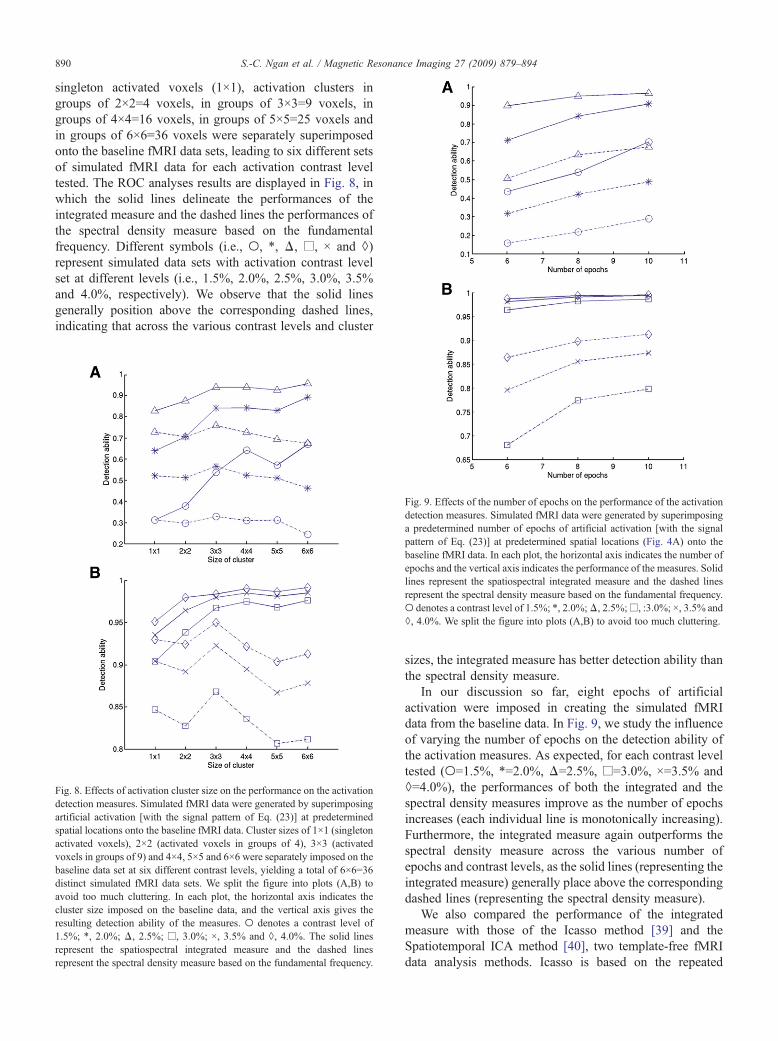
singleton activated voxels (1×1), activation clusters ingroups of 2×2=4 voxels, in groups of 3×3=9 voxels, ingroups of 4×4=16 voxels, in groups of 5×5=25 voxels andin groups of 6×6=36 voxels were separately superimposedonto the baseline fMRI data sets, leading to six different setsof simulated fMRI data for each activation contrast leveltested. The ROC analyses results are displayed in Fig. 8, inwhich the solid lines delineate the performances of theintegrated measure and the dashed lines the performances ofthe spectral density measure based on the fundamentalfrequency. Different symbols (i.e., ○, *, Δ, □, × and ◊)represent simulated data sets with activation contrast levelset at different levels (i.e., 1.5%, 2.0%, 2.5%, 3.0%, 3.5%and 4.0%, respectively). We observe that the solid linesgenerally position above the corresponding dashed lines,indicating that across the various contrast levels and cluster

Fig. 8. Effects of activation cluster size on the performance on the activationdetection measures. Simulated fMRI data were generated by superimposingartificial activation [with the signal pattern of Eq. (23)] at predeterminedspatial locations onto the baseline fMRI data. Cluster sizes of 1×1 (singletonactivated voxels), 2×2 (activated voxels in groups of 4), 3×3 (activatedvoxels in groups of 9) and 4×4, 5×5 and 6×6 were separately imposed on thebaseline data set at six different contrast levels, yielding a total of 6×6=36distinct simulated fMRI data sets. We split the figure into plots (A,B) toavoid too much cluttering. In each plot, the horizontal axis indicates thecluster size imposed on the baseline data, and the vertical axis gives theresulting detection ability of the measures. ○ denotes a contrast level of1.5%; *, 2.0%; Δ, 2.5%; □, 3.0%; ×, 3.5% and ◊, 4.0%. The solid linesrepresent the spatiospectral integrated measure and the dashed linesrepresent the spectral density measure based on the fundamental frequency.

Fig. 9. Effects of the number of epochs on the performance of the activationdetection measures. Simulated fMRI data were generated by superimposinga predetermined number of epochs of artificial activation [with the signalpattern of Eq. (23)] at predetermined spatial locations (Fig. 4A) onto thebaseline fMRI data. In each plot, the horizontal axis indicates the number ofepochs and the vertical axis indicates the performance of the measures. Solidlines represent the spatiospectral integrated measure and the dashed linesrepresent the spectral density measure based on the fundamental frequency.○ denotes a contrast level of 1.5%; *, 2.0%;Δ, 2.5%;□, :3.0%; ×, 3.5% and◊, 4.0%. We split the figure into plots (A,B) to avoid too much cluttering.

sizes, the integrated measure has better detection ability thanthe spectral density measure.

In our discussion so far, eight epochs of artificialactivation were imposed in creating the simulated fMRIdata from the baseline data. In Fig. 9, we study the influenceof varying the number of epochs on the detection ability ofthe activation measures. As expected, for each contrast leveltested (○=1.5%, *=2.0%, Δ=2.5%, □=3.0%, ×=3.5% and◊=4.0%), the performances of both the integrated and thespectral density measures improve as the number of epochsincreases (each individual line is monotonically increasing).Furthermore, the integrated measure again outperforms thespectral density measure across the various number ofepochs and contrast levels, as the solid lines (representing theintegrated measure) generally place above the correspondingdashed lines (representing the spectral density measure).

We also compared the performance of the integratedmeasure with those of the Icasso method [39] and theSpatiotemporal ICA method [40], two template-free fMRIdata analysis methods. Icasso is based on the repeated


application of the FastICA algorithm [41] and the clusteringof the results to enhance the reliability of the obtainedcomponents. (We applied resampling 25 times and employedthe Gaussian function as the nonlinearity function in theirfixed point algorithm. The other two nonlinearity functionsavailable in their software package gave the worse

Fig. 10. Comparison of the spatiospectral integrated detection measure withother template-free data analysis methods. To generate simulated fMRI datasets, three different types of temporal activation signal patterns [signalpattern of Eq. (23), boxcar and half-sinusoid] were used, leading tothe results in (A), (B) and (C) respectively. The horizontal axes indicate thecontrast level of the artificial activation imposed on the baseline data, and thevertical axes indicate the detection ability of the various measures.○ depictsthe performance of the spatiospectral integrated detection measure; *, theperformance of the Icasso method and Δ, the performance of theSpatiotemporal ICA method.

Fig. 11. Comparison of the three figures of merit. ○ indicates theperformance of the integrated measure optimized using the figure of meriof Eq. (18) * that optimized using the figure of merit of Eq. (20) and Δ thaoptimized using the figure of merit of Eq. (21). The detection abilities of thethree versions are very similar and hence the corresponding lines virtuallyoverlap.□ indicates the performance of P( fM/2

act). As before, simulated fMRdata sets were generated by superimposing artificial activations [of the signapattern of Eq. (23)] at pre-determined spatial locations (Fig. 4A) on thebaseline fMRI data.

tt

Il

performance for our data sets.) The Spatiotemporal ICAmethod simultaneously maximizes statistical independenceof the components temporally and spatially. (We used thedefault parameters with the skew spatial-temporal ICAoption and with α=0.5.) Each execution of the Icasso method(as well as the Spatiotemporal method) results in a number ofindependent components. To find the component most


relevant to activation, we calculate the correlation of the eachof the resulting components with the true spatial activationtemplate (i.e., Fig. 4A) and select the component with thebest correlation, yielding the performance results in Fig. 10(○:integrated measure, *:Icasso, Δ:Spatiotemporal ICA).The ROC analyses were done over seven different activationcontrast levels (1–4%) and three different types of temporalactivation signal pattern [Fig. 10A: pattern of Eq. (23), 10B:boxcar, 10C: half-sinusoid]. We see that the integrateddetection measure generally outperforms the Icasso and theSpatiotemporal ICA methods, except for the case with thecontrast level at 1.5% in subplot (c).

In all the analyses discussed thus far in this section, theintegrated detection measure Eq. (26) was optimized with thefigure of merit described in Eq. (18). When we instead usedthe figure of merits described in Eqs. (20) and (21) tooptimize the integrated measure, the resulting detectionabilities are very similar. For example, Fig. 11 shows theperformances of the integrated measure optimized with Eq.(18) (denoted by ○), that optimized with Eq. (20) (denotedby *), and that optimized with Eq. (21) (denoted by Δ).Again, the analyses were done over various contrast levelsand three temporal activation signal patterns, leading to thethree subplots. These lines largely overlap with one another

Fig. 12. Application of the activation detection measures to an experimentalfMRI data set. The data set was collected from a subject undergoing avisually cued motor paradigm. Eight epochs of the data were used. Panel (A)is the activation map generated by the integrated detection measure using a pvalue of .005, while (B) is the map generated using the spectral densitymeasure based on the fundamental frequency. Panels (C) and (D) are mapsgenerated using the Icasso method and the Spatiotemporal ICA method,respectively.

for the various contrast levels and activation signal patternstested. Lines with □ indicate the detection ability of P(fM/2

act )and are included in the figure to serve as a reference.

3.2. Using the activation detection measures onexperimental data

In Fig. 12, we depict the results of applying the integrateddetection measure, the spectral density measure, the Icassomethod and the Spatiotemporal ICA method on an experi-mental data set obtained from a visually cued motorparadigm. Using the procedure described in the Methodssection to generate the null histogram for the integratedmeasure, a threshold corresponding to a p value of .005 waschosen. Fig. 12A displays the corresponding activation map,which shows activation in both the V1 and M1 regions. Atotal of 90 voxels pass that threshold and are highlighted inthe figure. On the other hand, the 90 best scoring voxelsbased on their spectral density measure values at thefundamental frequency are highlighted in Fig. 12B.Fig. 12C, D show the top 90 voxels (in terms of voxelintensity) in the activation related independent componentsgenerated by the Icasso and Spatiotemporal methodsrespectively. On the whole, Fig. 12 shows that qualitatively,the activation map produced by the integrated measure is lessnoisy than the other three maps, in agreement with thequantitative assessment obtained from the ROC analyses ofthe simulated fMRI data.

4. Conclusion

In this article, we have improved upon a spectral densitybased activation detection measure for event-related fMRIdata by constructing a new, integrated detection measure.The spectral density-based measure estimates the degree oftask/stimulus related activation in a brain voxel by calculat-ing the spectral density at the fundamental frequency of aperiodic experimental paradigm. The new measure, termedthe spatiospectral integrated measure, linearly combines thespectral densities at the fundamental frequency and theharmonics and a spatial correlation term. Furthermore,several figures of merit have been described and used todetermine appropriate values for the coefficients in such alinear combination.

The motivation for extending the original spectral densitybased measure is that additional information regarding task/stimulus related activation in the fMRI data may becontained in and extractable from the first and higherharmonics of the experimental paradigm. Moreover, manypast fMRI studies have indicated the benefits of exploitingvoxel connectivity in data analysis because the sitescorresponding to neuronal activities often exist as spatialclusters rather than occur in isolation.

We have used both simulated fMRI and experimentalfMRI data to illustrate the utility of the spatiospectralintegrated detection measure. A variety of simulated fMRI


data sets were generated by superimposing artificial activa-tion of various temporal signal patterns with various contrastlevels at various spatial locations onto baseline fMRI data.ROC analysis of the results quantified and demonstrated theimproved detection ability of the integrated measure over theoriginal spectral density based measure over a range oftesting conditions. Our experimental fMRI data obtainedusing a visually guided motor paradigm depicted qualita-tively that we can obtain a more sensitive and specificactivation map using the new measure. The present measurealso compares quite favorably with the Spatiotemporal ICAand the Icasso methods, which are useful template-free fMRIdata analysis methods themselves.

The present method depends on the existence ofreproducible response patterns across epochs. Fortunately,even with this limitation, the method is still applicable tofMRI data sets obtained from a large subclass of usefulexperimental paradigms. The performances of the integratedas well as the purely spectral density based measures will ofcourse deteriorate if the activation patterns in the epochs arenot exactly in phase, with the degree of reduction dependentupon how out of phase the activation patterns are. For thegeneration of null data sets under these circumstances,resampling techniques such as wavelet resampling [42,43]can be applied as an additional step after the pairing andsubtraction procedure described in Eq. (4.1) to furtherremove any residual activation signals.

Finally, the integrated measure can be expanded toinclude terms other than the spectral densities and the spatialcorrelation. For example, the statistical map generated fromthe present integrated measure can be used to identify theactivation related independent components obtained fromthe Icasso and the Spatiotemporal ICA methods. Thestatistical map and the components can then be combinedlinearly to produce a further improved activation map. Acaveat is that overfitting might possibly occur if we includetoo many terms in the integrated measure. Fortunately, thisproblem can be overcome by testing whether the coefficientfor each term is significantly different from zero usingresampling or cross-validation. Moreover, moving awayfrom the domain of spectral densities, we can utilize thefigures of merit to choose an appropriate subset of waveletbasis in the wavelet analysis of event-related fMRI data, tochoose appropriate kernel width for spatial smoothing offMRI data (Refs. [44–46] are examples of attempts infinding optimal spatial smoothing) and to determine anoptimal neighborhood size for the computing spatialcorrelation measure [referring to Eq. (12), we currentlyimpose a neighborhood size of Q=4 for single slice data].Some of these topics will be discussed in a separate article.

Acknowledgments

The authors thank the anonymous reviewers for their veryhelpful suggestions and comments. SCN thanks W. Auffer-mann for past discussions on fMRI data analysis. This

research is supported by a University of Hong Kong grant200707176135 to SCN.

References

[1] Bandettini PA, Jesmanowicz A, Wong EC, Hyde JS. Processingstrategies for time-course data sets in functional MRI of the humanbrain. Magn Reson Med 1993;30:161–73.

[2] Friston KJ, Jezzard P, Turner R. Analysis of functional MRI time-series. Hum Brain Mapp 1994;1:153–71.

[3] Rosen BR, Buckner RL, Dale AM. Event-related functional MRI: past,present, and future. Proc Natl Acad Sci U S A 1998;95:773–80.

[4] Buckner RL, Badettini PA, O'Craven KM, Savoy RL, Peterson SE,Raichle ME, et al. Detection of cortical activation during averagedsingle trials of a cognitive task using functional magnetic resonanceimaging. Proc Natl Acad Sci U S A 1996;93:14878–83.

[5] Zarahn E, Aguirre G, D'Esposito M. A trial-based experimental designfor fMRI. Neuroimage 1997;6:122–38.

[6] Liu TT, Frank LR, Wong EC, Buxton RB. Detection power, estimationefficiency, and predictability in event-related fMRI. Neuroimage2001;13:759–73.

[7] Hu X, Le TH, Ugurbil K. Evaluation of the early response in fMRI inindividual subjects using short stimulus duration. Magn Reson Med1997;37:877–84.

[8] Kato T, Erhard P, TakayamaY, Strupp J, Le TH,Ogawa S, et al. Cerebralmultiphasic sustained responses (CMSR) in memory processing:detection of hippocampal long-term sustained response using fMRI at4 Tesla. Fifth Annual Meeting of the International Society for MagneticResonance in Medicine: 1997. Vancouver, Canada: InternationalSocieyt for Magnetic Resonance in Medicine; 1997. p. 12.

[9] Richter W, Andersen PM, Georgopoulos AP, Kim SG. Time resolvedfMRI of mental rotation. Neuroreport 1997;8:3697–702.

[10] Richter W, Andersen PM, Georgopoulos AP, Kim SG. Sequentialactivity in human motor areas during a delayed cued fingermovement task studied by time-resolved fMRI. Neuroreport1997;8:1257–61.

[11] Ngan SC, Hu X. Analysis of functional magnetic resonance imagingdata during self-organizing mapping with spatial connectivity. MagnReson Med 1999;41:939–46.

[12] Ding X, Tkach J, Ruggieri P, Masaryk T. Analysis of time-coursefunctional MRI data with clustering method without the use ofreference signal. Second Annual Meeting of the International Societyfor Magnetic Resonance in Medicine: 1994. San Francisco:International Society for Magnetic Resonance in Medicine; 1994.p. 630.

[13] Scarth G, McIntyre M, Wouk B, Somorjai RL. Detection of novelty infunctional images using fuzzy clustering. Third Annual Meeting of theInternational Society for Magnetic Resonance in Medicine: 1995.Nice, France: International Society for Magnetic Resonance inMedicine; 1995. p. 238.

[14] Baumgartner G, Scarth G, Teichtmeister C, Somorjai RL, Moser E.Fuzzy clustering of gradient-echo functional MRI in the humanvisual cortex. Part I: reproducibility. J Magn Reson Imag 1997;7:1094–101.

[15] Fischer H, Hennig J. Neural network-based analysis of MR time series.Magn Reson Med 1999;41:124–31.

[16] Golay X, Kollias S, Stoll G, Meier D, Valavanis A, Boesiger P. A newcorrelation-based fuzzy logic clustering algorithm for fMRI. MagnReson Med 1998;40:249–60.

[17] Voultsidou M, Dodel S, Herrmann JM. Neural networks approach toclustering of activity in fMRI data. IEEE Trans on Med Imag 2005;24(8):987–96.

[18] McKeown MJ, Jung TP, Makeig S, Brown G, Kindermann SS, LeeTW, et al. Spatially independent activity patterns in functionalmagnetic resonance imaging data during the Stroop color-namingtask. Proc Natl Acad Sci U S A 1998;95:803–10.


[19] Moeller JR, Strother SC. A regional covariance approach to theanalysis of functional patterns in positron emission tomographic data. JCereb Blood Flow Metab 1991;11:A121–35.

[20] Beckmann CF, Smith SM. Probabilistic independent componentanalysis for functional magnetic resonance imaging. IEEE TransMed Imag 2004;23:137–52.

[21] Moritz CH, Rogers BP, Meyerand ME. Power spectrum rankedindependent component analysis of a periodic fMRI complex motorparadigm. Hum Brain Mapp 2003;18:111–22.

[22] Formisano E, Esposito F, Di Salle F, Goebel R. Cortex-basedindependent component analysis of fMRI time series. Magn ResonImag 2004;22(10):1493–504.

[23] Shen X,Meyer FG. Analysis of event-related fMRI data using diffusionmaps. In: Christensen GE, SonkaM, editors. Information Processing inMedical Imaging, vol. 3565. Berlin: Springer; 2005. p. 652–63.

[24] Thirion B, Dodel S, Poline JB. Detection of signal synchronization inresting-state fMRI datasets. Neuroimage 2006;29:321–7.

[25] Mitra PP, Pesaran B. Analysis of dynamic brain imaging data.Biophysical J 1999;76:691–708.

[26] Marchini JL, Ripley BD. A new statistical approach to detectingsignificant activation in functional MRI. Neuroimage 2000;12:366–80.

[27] Wong EC, Buxton RB, Blaettler D, Frank LR. Unbiased identifica-tion of functionally distinct groups of pixels in functional MRI usingcluster analysis in Fourier space. Third Annual meeting of theInternational Society for Magnetic Resonance in Medicine. Nice,France: International Society for Magnetic Resonance in Medicine;1993. p. 825.

[28] Engel SA, Rumelhart DE, Wandell BA, Lee AT, Glover GH,Chichilnisky EJ, et al. fMRI of human visual cortex. Nature1994;369:525.

[29] Soreno MI, Dale AM, Reppas JR, Kwong KK, Belliveau JW, BradyTJ, et al. Functional MRI reveals borders of multiple visual areas inhumans. Science 1995;268:889–93.

[30] Forman SD, Cohen JD, Fitzgerald M, EddyWF, Mintun MA, Noll DC.Improved assessment of significant change in functional magneticresonance imaging (fMRI): use of a cluster size threshold. Magn ResonMed 1995;33:636–47.

[31] Betrand O, Bohorquez J, Pernier J. Time-frequency digital filteringbased on an invertible wavelet transform: an application to evokedpotentials. IEEE Trans Biomed Eng 1994;41:77–84.

[32] de Weerd JPC, Kap JI. A posteriori time-varying filtering of averagedevoked potentials. II. Mathematical and computational aspects. BiolCybern 1981;41:211–22.

[33] Friston KJ, Worsley KJ, Frackowiak RSJ, Mazziotta JC, Evans AC.Assessing the significance of focal activations using their spatialextent. Hum Brain Mapp 1994;1:210–20.

[34] Xiong J, Gao JH, Lancaster JL, Fox PT. Clustered pixels analysis forfunctional MRI activation studies of the human brain. Hum BrainMapp 1995;3:287–301.

[35] Hayasaka S, Luan PK, Liberzon I, Worsley KJ, Nichols TE.Nonstationary cluster-size inference with random field and permuta-tion methods. NeuroImage 2004;22:676–87.

[36] Worsley KJ, Marrett S, Neelin P, Vandal AC, Friston KJ, Evans AC. Aunified statistical approach for determining significant signals inimages of cerebral activation. Hum Brain Mapp 1996;4:58–73.

[37] Nandy R, Cordes D. Novel ROC-type method for testing the efficiencyof multivariate statistical methods in fMRI. Magn Reson Med 2003;49:1152–62.

[38] Xiong J, Gao JH, Lancaster JL, Fox PT. Assessment and optimizationof functional MRI analyses. Hum Brain Mapp 1996;4:153–67.

[39] Himberg J, Hyvarinen A, Esposito F. Validating the independentcomponents of neuroimaging time-series via clustering and visualiza-tion. Neuroimage 2004;22:1214–22.

[40] Stone JV, Porrill J, Porter NR, Wilkinson ID. Spatiotemporalindependent component analysis of event-related fMRI data usingskewed probability density functions. Neuroimage 2002;15:407–21.

[41] Hyvarinen A, Oja E. Independent component analysis: algorithms andapplications. Neural Networks 2000;13:411–30.

[42] Breakspear M, Brammer MJ, Bullmore ET, Das P, Williams LM.Spatiotemporal wavelet resampling for functional neuroimaging data.Hum Brain Mapp 2004;23:1–25.

[43] Bullmore E, Long C, Suckling J, Fadili J, Calvert G, Zelaya F, et al.Colored noise and computational inference in neurophysiological timeseries analysis: resampling methods in time and wavelet domains. HumBrain Mapp 2001;12:61–78.

[44] Jo HJ, Lee JM, Kim JH, Shin YW, Kim IY, Kwon JS, et al. Spatialaccuracy of fMRI activation influenced by volume-and surface-basedspatial smoothing techniques. Neuroimage 2007;34:550–64.

[45] Shaw ME, Strother SC, Gavrilescu M, Podzebenko K, Waites A,Watson J, et al. Evaluating subject specific preprocessing choices inmultisubject fMRI data sets using data-driven performance metrics.Neuroimage 2003;19:988–1001.

[46] LaConte S, Anderson J, Muley S, Ashe J, Frutiger S, Rehm K, et al.The evaluation of preprocessing choices in single-subject BOLDfMRI using NPAIRS performance metrics. Neuroimage 2003;18:10–27.

improvement of spectral density-based activation … of spectral density...improvement of spectral...

Documents