improving frequentist prediction intervals for ar models by simulation

Introduction and motivation Prediction formulae Regression and autoregression Bayesian prediction Generalization Sim

Improving frequentist prediction intervals forAR models by simulation

J. Helske and J. Nyblom

Department of Mathematics and StatisticsUniversity of Jyvaskyla

Oxford 29–30 June, 2010

J. Helske and J. Nyblom Improved prediction intervals


Table of contents

1 Introduction and motivation

2 Prediction formulae

3 Regression and autoregression

4 Bayesian prediction

5 Generalization

6 Simulations

7 Example

8 References



Criticism

Chatfield(1993): Reasons why a prediction interval may bewrong

Parameters are estimated.

Errors are not normally distributed.

The model is wrong.

The model will change in the future.

Here we consider the first issue.



Some earlier work for AR models

Focus on prediction mean squared error (analytic andbootstrap):

Phillips(1979), J of EconometricsFuller and Hasza (1981), JASAAnsley and Kohn (1986), BiometrikaQuenneville and Singh (2002), JTSAPfeffermann and Tiller (2005), JTSA



Some earlier work for AR models

Prediction interval with estimated parameters:

Barndorff-Nielsen and Cox (1996), BernoulliVidoni (2004, 2009), JTSA

Bootstrap solutions:

Beran (1990), JASAMasarotto (1990), Int. J. of ForecastingGrigoletto (1998), Int. J. of ForecastingKim (2004), Int. J. of ForecastingPascual, Romo and Ruiz (2004), JTSAClements and Kim (2007), Comp. Stat. & Data Anal.Kabaila and Syuhada (2008), JTSARodrıguez and Ruiz (2009), JTSA



AR(1): One step ahead

−0.5 0.0 0.5

0.85

0.86

0.87

0.88

0.89

0.90

0.91

β1

Cov

erag

e pr

obab

ility

−0.9 −0.5 0.5 0.9

yt = β0 + β1yt−1 + εt , εt ∼ NID(0, σ2), t = 1, . . . , 30.Goal: 90 % prediction intervalUpper = New, Lower = Standard.Based on a simulation study.



AR(1): Formulae: parameters known

Prediction interval, 1 step ahead:

β0 + β1yn ± σzα,

Prediction interval, k step ahead:

β01 − βk

1

1 − β1+ βk

1 yn ± σ

√1 − β2k

1

1 − β21

zα.

Lower limit = L(y ,θ), upper limit = U(y ,θ), θ = (β0, β1, σ)′,

Pθ(L(y ,θ) ≤ yn+k ≤ U(y ,θ) | y) = 1 − 2α.



AR(1): Frequentist coverage probability

Parameter estimates θ = θ(y).

Pθ(L(y , θ) ≤ yn+k ≤ U(y , θ) | y)

varies across samples (and also with parameters)!Goal

Eθ

[P(L(y , θ) ≤ yn+k ≤ U(y , θ) | y)

]= 1 − 2α (1)

or at least ≈ 1 − 2α for all θ.

Equation (1) means that the frequentist coverage probabilityis 1 − 2α, i.e. in repeated hypothetical samples from thesame AR(1) the p.i.’s contain the future values with probability1 − 2α on the average.



Standard p.i.’s conditionally: one step ahead

Pθ(L(y , θ) ≤ yn+k ≤ U(y , θ) | y)

Coverage probability

Den

sity

0.3 0.4 0.5 0.6 0.7 0.8 0.9 1.0

02

46

8

50000 replicates from AR(1) with β1 = 0.8, n = 30,1 − 2α = 0.9, mean = 0.871.



Ordinary linear regression

Linear regression

yt = x ′tβ + εt , x t fixed, t = 1, . . . , n.

Let xn+1 known. The usual prediction interval for yn+1

x ′n+1β ± s

√1 + x ′

n+1(X′X )−1xn+1 tα;n−p−1, (2)

where X , n × (p + 1), has rows x ′t .

This interval satisfies

Eθ

[P(L(y , θ) ≤ yn+1 ≤ U(y , θ) | y)

]= 1 − 2α.

The frequentist coverage probability is exact!



Autoregression

Autoregression

yt = β0 + β1yt−1 + · · ·+ βpyt−p + εt

= x ′tβ + εt , x ′

t = (1, yt−1, . . . , yt−p), t = 1, . . . , n.

Least squares estimation conditionally on (y0, . . . , y−p+1) andthe prediction interval for yn+1 by analogy with OLS leads to

x ′n+1β ± s

√1 + x ′

n+1(X′X )−1xn+1 tα;n−p−1.




It works well!

−0.5 0.0 0.5

0.85

0.86

0.87

0.88

0.89

0.90

0.91

β1

Cov

erag

e pr

obab

ility

−0.9 −0.5 0.5 0.9

yt = β0 + β1yt−1 + εt , εt ∼ N(0, σ2), t = 1, . . . , 30.Upper = Regression formula, Lower = Standard formula.



What about AR(2) models?

Table: The models used in the simulation experiments.

r−11 r−1

2 β1 β2

0.9 0.5 1.4 −0.450.9 −0.5 0.4 0.45

−0.9 0.5 −0.4 0.45−0.9 −0.5 −1.4 −0.45

0.5 0.5 1.0 −0.250.5 −0.5 0 0.25

0.9 exp( i5) 0.9 exp(− i

5) 1.76 −0.810.9 exp( iπ

2 ) 0.9 exp(− iπ2 ) 0 −0.81

0.9 exp( i3π4 ) 0.9 exp(− i3π

4 ) −1.27 −0.81

The values r1, r2 satisfy 1 − β1r − β2r2 = 0J. Helske and J. Nyblom Improved prediction intervals



It works well also here!

2 4 6 8

0.85

0.86

0.87

0.88

0.89

0.90

0.91

Models

Cov

erag

e pr

obab

ility

yt = β0 + β1yt−1 + β2yt−2 + εt , εt ∼ N(0, σ2), t = 1, . . . , 30.Upper = Regression formula, Lower = Standard formula.



Regression approach seems to solve one step aheadprediction problem. But what to do for 2 steps, 3 steps and soon prediction intervals?



Bayesian interpretation

Back to linear regression

x ′n+1β ± s

√1 + x ′

n+1(X′X )−1xn+1 tα;n−p−1.

Let us adopt the improper (diffuse) prior p(β, σ) = 1/σ. Then aposteriori

P(L(y , θ) ≤ yn+1 ≤ U(y , θ) | y) = 1 − 2α.



Likelihood, prior and posterior

Let X be as in autoregression, and y−p+1, . . . , y0 fixed. Thenthe likelihood is

p(y |β, σ) = (2π)−n2σ−(n−p−1) exp

(−(n − p − 1)s2

2σ2

)

×σ−p−1 exp(−

12σ2 (β − β)′(X ′X )(β − β)

).

Assume a priori p(β, σ) = 1/σ. Then the posterior distributionsare as in ordinary linear regression.

p(β, σ | y) ∝1σ

p(y |β, σ),

(n − p − 1)s2/σ2 | y ∼ χ2(n − p − 1),

β | y , σ ∼ N(β, σ2(X ′X )−1).



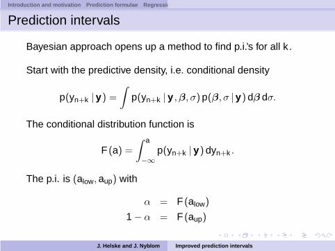
Prediction intervals

Bayesian approach opens up a method to find p.i.’s for all k .

Start with the predictive density, i.e. conditional density

p(yn+k | y) =∫

p(yn+k | y ,β, σ) p(β, σ | y) dβ dσ.

The conditional distribution function is

F (a) =∫ a

−∞p(yn+k | y) dyn+k .

The p.i. is (alow, aup) with

α = F (alow)

1 − α = F (aup)



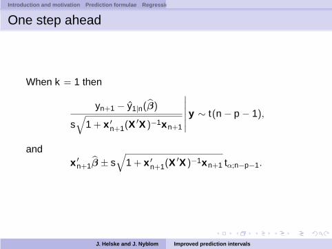
One step ahead

When k = 1 then

yn+1 − y1|n(β)

s√

1 + x ′n+1(X

′X )−1xn+1

∣∣∣∣∣∣y ∼ t(n − p − 1),

andx ′

n+1β ± s√

1 + x ′n+1(X

′X )−1xn+1 tα;n−p−1.



k steps ahead

When k > 1 we use simulation

Generate q1, . . . , qN independently from χ2(n − p − 1), andlet σ2

i = (n − p − 1)s2/qi .

Generate βi from N(β, σ2i (X

′X )−1) independentlyi = 1, . . . ,N.

Then

F (a) ≈1N

N∑

i=1

Φ

(a − yk |n(βi)

σivk |n(βi)

)



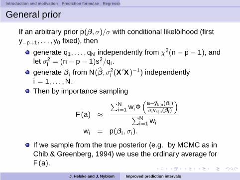
General prior

If an arbitrary prior p(β, σ)/σ with conditional likeloihood (firsty−p+1, . . . , y0 fixed), then

generate q1, . . . , qN independently from χ2(n − p − 1), andlet σ2

i = (n − p − 1)s2/qi .

generate βi from N(β, σ2i (X

′X )−1) independentlyi = 1, . . . ,N.Then by importance sampling

F (a) ≈

∑Ni=1 wiΦ

(a−yk|n(βi )

σi vk|n(βi )

)

∑Ni=1 wi

wi = p(βi , σi).

If we sample from the true posterior (e.g. by MCMC as inChib & Greenberg, 1994) we use the ordinary average forF (a).



The first values revisited

Let ps(y0 |β, σ) be the stationary density of(y−p+1, . . . , y0)

′ = y0, then combining the prior with the exactlikelihood leads to the weights

wi = ps(y0 |βi , σi)p(βi , σi).

The benefit of the inportance sampling is a fairly simple formulafor the Monte Carlo error.



Examples of priors for AR(1)

p(β, σ)σ

=1σ, uniform,

=I(|β1| < 1)

σ, uniform stationary,

=I(|β1| < 1)

πσ√

1 − β21

, Jeffreys,

=I(|β1| < 1)

2πσ√

1 − β21

+I(|β1| > 1)

2πσ|β1|√β2

1 − 1, reference.

The reference prior is due to Berger and Yang (1994).



Our goal is to find priors that produce p.i.’s havingapproximately correct frequentist coverage probabilites.

Probability matching priors:Datta and Mukerjee (2003, 2004), AISM, monograph



Multistep predictions

2 4 6 8 10

0.60

0.70

0.80

0.90

β1 = − 0.5

2 4 6 8 10

0.60

0.70

0.80

0.90

β1 = 0.5

2 4 6 8 10

0.60

0.70

0.80

0.90

β1 = 0.7

2 4 6 8 100.

600.

700.

800.

90

β1 = 0.9

Cov

erag

e pr

obab

ility

Lead

Figure: Coverage probabilities, AR(1), n = 30, 1 − 2α = 0.9. Dashed blackline = refrence, dotted line = standard, uniform = solid grey, Jeffreys = greydashed, and uniform stationary = black dot-and-dash.



2 4 6 8 100.

600.

750.

90

r1−1 = 0.9, r2

−1 = 0.5

2 4 6 8 10

0.60

0.75

0.90

r1−1 = 0.9, r2

−1 = − 0.5

2 4 6 8 10

0.60

0.75

0.90

r1−1 = − 0.9, r2

−1 = 0.5

2 4 6 8 10

0.60

0.75

0.90

r1−1 = − 0.9, r2

−1 = − 0.5

2 4 6 8 10

0.60

0.75

0.90

r1−1 = 0.5, r2

−1 = 0.5

2 4 6 8 10

0.60

0.75

0.90

r1−1 = 0.5, r2

−1 = − 0.5

2 4 6 8 10

0.60

0.75

0.90

r1, 2−1 = 0.9exp( ± i0.2)

2 4 6 8 10

0.60

0.75

0.90

r1, 2−1 = 0.9exp( ± iπ 2)

2 4 6 8 10

0.60

0.75

0.90

r1, 2−1 = 0.9exp( ± i3π 4)

Cov

erag

e pr

obab

ility

Lead

Figure: The coverage probabilities of AR(2)-processes with n = 30,1 − 2α = 0.9 and roots r1, r2. Black dotted = standard, solid grey = uniform,grey dashed = Jeffreys, and dotted-and-dashed = uniform stationary prior.



0.0 0.5 1.0 1.5 2.0 2.5 3.0

02

46

r1−1 = 0.9, r2

−1 = 0.5

0.0 0.5 1.0 1.5 2.0 2.5 3.0

02

46

r1−1 = 0.9, r2

−1 = − 0.5

0.0 0.5 1.0 1.5 2.0 2.5 3.0

02

46

r1−1 = − 0.9, r2

−1 = 0.5

0.0 0.5 1.0 1.5 2.0 2.5 3.0

02

46

r1−1 = − 0.9, r2

−1 = − 0.5

0.0 0.5 1.0 1.5 2.0 2.5 3.0

02

46

r1−1 = 0.5, r2

−1 = 0.5

0.0 0.5 1.0 1.5 2.0 2.5 3.0

02

46

r1−1 = 0.5, r2

−1 = − 0.5

0.0 0.5 1.0 1.5 2.0 2.5 3.0

02

46

r1, 2−1 = 0.9exp( ± i0.2)

0.0 0.5 1.0 1.5 2.0 2.5 3.0

02

46

r1, 2−1 = 0.9exp( ± iπ 2)

0.0 0.5 1.0 1.5 2.0 2.5 3.0

02

46

r1, 2−1 = 0.9exp( ± i3π 4)

Frequency

Val

ue

Figure: The scaled spectral density functions of the nine AR(2)-processesfrom Table 1.



0 5 10 15

−1.

00.

01.

0

r1−1 = 0.9, r2

−1 = 0.5

0 5 10 15

−1.

00.

01.

0

r1−1 = 0.9, r2

−1 = − 0.5

0 5 10 15

−1.

00.

01.

0

r1−1 = − 0.9, r2

−1 = 0.5

0 5 10 15

−1.

00.

01.

0

r1−1 = − 0.9, r2

−1 = − 0.5

0 5 10 15

−1.

00.

01.

0

r1−1 = 0.5, r2

−1 = 0.5

0 5 10 15

−1.

00.

01.

0

r1−1 = 0.5, r2

−1 = − 0.5

0 5 10 15

−1.

00.

01.

0

r1, 2−1 = 0.9exp( ± i0.2)

0 5 10 15

−1.

00.

01.

0

r1, 2−1 = 0.9exp( ± iπ 2)

0 5 10 15

−1.

00.

01.

0

r1, 2−1 = 0.9exp( ± i3π 4)

AC

F

Lag

Figure: The autocorrelation functions of the nine AR(2)-processes.



2 4 6 8 10

0.70

0.80

0.90

1.00

r1−1 = 0.9, r2

−1 = 0.5

2 4 6 8 10

0.70

0.80

0.90

1.00

r1−1 = 0.9, r2

−1 = − 0.5

2 4 6 8 10

0.70

0.80

0.90

1.00

0.9exp( ± i0.2)

Cove

rage

pro

babil

ities

Lead

Figure: Coverage probabilities for 3 AR(2) processes, n = 50, 1 − 2α = 0.9.Dashed black line = refrence and the bottom dotted line = standard, uniform =solid dark grey, Jeffreys = light grey dashed, and uniform stationary = blackdot-and-dash.



Annual consumer price inflation in the United Kingdom (UK)and United States (US).http://data.worldbank.org/indicator/fp.cpi.totl.zg.

Based on autocorrelations and partial autocorrelations weassumeAR(1) model for the UK series,AR(3) model for the US series.



Model fit 1961–1999. Forecast period 2000-2009.

β0 β1 β2 β3 σ r−11 r−1

2,3UK 1.40 0.80 3.29 0.80US 0.92 1.32 -0.90 0.40 1.54 0.82 0.7 exp(±i1.21)



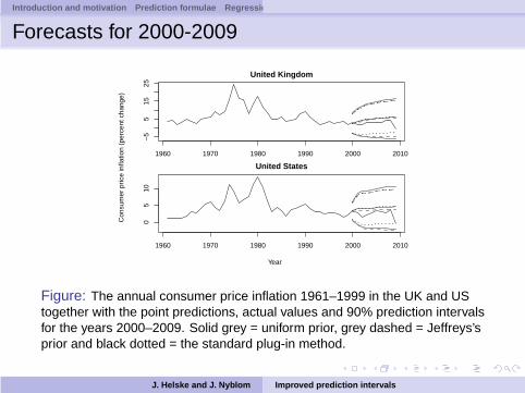
Forecasts for 2000-2009

United Kingdom

1960 1970 1980 1990 2000 2010−

55

1525

United States

1960 1970 1980 1990 2000 2010

05

10

Con

sum

er p

rice

infla

tion

(per

cent

cha

nge)

Year

Figure: The annual consumer price inflation 1961–1999 in the UK and UStogether with the point predictions, actual values and 90% prediction intervalsfor the years 2000–2009. Solid grey = uniform prior, grey dashed = Jeffreys’sprior and black dotted = the standard plug-in method.



Model fit 1961–2009. Forecast period 2010-2014.

β0 β1 β2 β3 σ r−11 r−1

2,3UK 1.03 0.82 – – 3.02 0.82 –US 0.65 1.27 -0.82 0.39 1.58 0.82 0.68 exp(±i1.25)



Forecasts for 2010–2014

United Kingdom

1995 2000 2005 2010

−5

05

10

United States

1995 2000 2005 2010

−4

04

Con

sum

er p

rice

infla

tion

(per

cent

cha

nge)

Year

Figure: The annual consumer price inflation 1995–2009 and its predictionswith prediction intervals 2010–2014. The colors dark to light represent the50%, 75% and 90% intervals with Jeffreys’s prior.



Predictive densities

−10 −5 0 5 10

0.00

0.02

0.04

0.06

0.08

0.10

0.12

0.14

Inflation

Den

sity

Figure: Predictive densities of the US inflation for 2014 (5 steps ahead).Black = Standard, Blue = uniform prior, Red = Jeffreys’s prior.



Table: Coverage probability checks and prediction limits with standarderrors, for the UK and US consumer price inflation series 1961-1999.

Bayes with uniform prior Bayes with Jeffreys’s priork = 1 k = 5 k = 10 k = 1 k = 5 k = 10

United KingdomCoverage 0.898 0.869 0.867 0.897 0.871 0.869b1−α 8.343 14.270 16.449 8.165 13.670 15.469s.e.(b1−α) – 0.008 0.013 0.003 0.006 0.009bα -3.068 -5.335 -6.113 -3.032 -4.913 -5.180s.e.(bα) – 0.017 0.031 0.003 0.011 0.017

United StatesCoverage 0.899 0.891 0.898 0.897 0.893 0.900b1−α 6.035 9.495 10.623 5.745 8.828 9.663s.e.(b1−α) – 0.006 0.008 0.002 0.006 0.007bα 0.649 -1.636 -2.028 0.550 -2.042 -2.457s.e.(bα) – 0.008 0.014 0.002 0.007 0.010



Spectral densities

0.0 0.5 1.0 1.5 2.0 2.5 3.0

0.0

0.5

1.0

1.5

2.0

2.5

Frequency

Val

ue

Figure: Spectral densities for the fitted models; Black = UK, Blue = US.



References close to our approach:

Zellner (1971), monographBroemeling and Land (1984), Comm. in Stat.Thompson and Miller (1986), JBESLiu (1994), AISMSnyder, Ord, Koehler (2001), JBES



Our method:

Almost exact for 1 step ahead predictions.

Easy to implement and to understand.

Computationally fast.

Simple expression for simulation error.

Easy to check the performance of the fitted model.

Performance worse when– long forecast horizons– major spectral mass on low frequences.



References

Ansley, C. F. and Kohn, R., (1986). Prediction Mean SquaredError for State Space Models With Estimated Parameters,Biometrika, 73, 467–473.

Barndorff-Nielsen, O. E. and Cox, D. R. (1996). Prediction andAsymptotics, Bernoulli, 2, 319–340.

Beran, R. (1990). Calibrating Prediction Regions, Journal of theAmerican Statistical Association, 85, 715–723.

Berger, J. O. and Yang, R. (1994). Noninformative Priors andBayesian Testing for the AR(1) Model, Econometric Theory,10, 461–482.

Berger, J. (2006). The Case of Objective Bayesian Analysis,Bayesian Analysis, 1, 385–402.



Box, G. E. P. and Jenkins, G. M. and Reinsel, G. C. (2008).Time Series Analysis: Forecasting and Control, New York:Wiley.

Broemeling, L. and Land, M. (1984). On Forecasting WithUnivariate Autoregressive Processes: A BayesianApproach, Communications in Statistics — Theory andMethods, 13, 1305–1320.

Chow, G.C. (1975). Multiperiod predictions from stochasticdifference equations by Bayesian methods, Econometrica,41, 109–118.

Chatfield, C. (1993). Calculating Interval Forecasts, Journal ofBusiness & Economic Statistics, 11, 121–135.

Chatfield, C. (1996). Model Uncertainty and Forecast Accuracy,Journal of Forecasting, 15, 495–508.



Chib, S. and Greenberg, E. (1994). Bayes inference inregression models with ARMA(p, q) errors. Journal ofEconometrics, 64, 183–206.

Clements, M. P. and Kim, J. H. (2007). Bootstrap PredictionIntervals for Autoregressive Time Series, ComputationalStatistics & Data Analysis, 51, 3580–3594.

Fuller, W. A and Hasza, D. (1981). Properties of Predictors forAutoregressive Time Series, Journal of the AmericanStatistical Association, 76, 155–161.

Datta, G. and Mukerjee, R. (2003). Probability Matching Priorsfor Predicting a Dependent Variable With Application toRegression Models, Annals of the Institute of StatisticalMathematics, 55, 1–6.



Datta, G. and Mukerjee, R. (2004). Probability Matching Priors:Higher Order Asymptotics, New York: Springer.

Ghosh, M. and Heo, J. (2003). Default Bayesian Priors forRegression Models With First-Order AutoregressiveResiduals, Journal of Time Series Analysis, 24, 269–282.

Grigoletto, M. (1998). Bootstrap Prediction Intervals forAutoregressions: Some Alternatives, International Journalof Forecasting, 14, 447–456.

Kabaila, P. and Syuhada, K. (2008). Improved Prediction Limitsfor AR(p) and ARCH(p) processes, Journal of Time SeriesAnalysis, 29, 213–223.

Kim, J. H. (2004). Bootstrap Prediction Intervals forAutoregression Using Asymptotically Mean-UnbiasedEstimators, International Journal of Forecasting, 20, 85–97.



Liu, S. I. (1994). Multiperiod Bayesian Forecasts for ARModels, Annals of the Institute of Statistical Mathematics,46, 429–452.

Masarotto, G. (1990). Bootstrap Prediction Intervals forAutoregressions, International Journal of Forecasting, 6,229–239.

Pascual, L. and Romo, J. and Ruiz, E. (2004). BootstrapPredictive Inference for ARIMA Processes, Journal of TimeSeries Analysis, 25, 449–465.

Phillips, P. C. B. (1979). The Sampling Distribution of ForecastsFrom a First-Order Autoregression, Journal ofEconometrics, 9, 241–261.

Pfeffermann, D. and Tiller, R. (2005). Bootstrap Approximationto Prediction MSE for State-Space Models With EstimatedParameters, Journal of Time Series Analysis, 26, 893–916.



Quenneville, B. and Singh, A. C. (2000). Bayesian PredictionMean Squared Error for State Space Models WithEstimated Parameters, Journal of Time Series Analysis,21, 219–236.

Rodriguez, A. and Ruiz, E. (2009). Bootstrap PredictionIntervals in State-Space Models, Journal of Time SeriesAnalysis, 30, 167–178.

Snyder, R. D. and Ord, J. K. and Koehler, A. B. (2001).Prediction Intervals for ARIMA Models, Journal of Business& Economic Statistics, 19, 217–225.

Thompson, P. A. and Miller, R. B. (1986). Sampling the Future:A Bayesian Approach to Forecasting to Univariate TimeSeries Models, Journal of Business & Economic Statistics,4, 427–436.



Vidoni, P. (2004). Improved Prediction Intervals for StochasticProcess Models, Journal of Time Series Analysis, 25,137–154.

Vidoni, P. (2009). A Simple Procedure for Computing ImprovedPrediction Intervals for Autoregressive Models, Journal ofTime Series Analysis, 30, 577–590.

Zellner, A. (1971). An Introduction to Bayesian Inference inEconometrics, New York: Wiley.


improving frequentist prediction intervals for ar models by simulation

Documents