applied sciences

Article

Improving the Accuracy of Fault Frequency by Meansof Local Mean Decomposition and Ratio CorrectionMethod for Rolling Bearing Failure

Yongqiang Duan 1, Chengdong Wang 1,2,* , Yong Chen 1,2 and Peisen Liu 3

1 School of Automation Engineering, University of Electronic Science and Technology of China,Chengdu 611731, China; 15008257533@163.com (Y.D.); ychencd@uestc.edu.cn (Y.C.)

2 Institute of Electric Vehicle Driving System and Safety Technology,University of Electronic Science and Technology of China, Chengdu 611731, China

3 School of Mechanical Engineering, Chengdu Technological University, Chengdu 611730, China;liupeisen103@163.com

* Correspondence: wangchengdong@uestc.edu.cn

Received: 11 April 2019; Accepted: 2 May 2019; Published: 8 May 2019�����������������

Abstract: The fault frequencies are as they are and cannot be improved. One can only improveits estimation quality. This paper proposes a fault diagnosis method by combining local meandecomposition (LMD) and the ratio correction method to process the short-time signals. Firstly,the vibration signal of rolling bearing is decomposed into a series of product functions (PFs) byLMD. The PF, which contains the richest fault information, is selected to perform envelope spectrumanalysis by the Hilbert transform (HT). Secondly, the Hilbert envelope spectrum of the selected PF iscorrected with the ratio correction method. Finally, higher precision fault frequencies are extractedfrom the corrected Hilbert envelope spectrum, and then the fault location is accurately determined.The proposed method of this paper can be used in online real-time monitoring technology of rollingbearing failure.

Keywords: local mean decomposition; spectrum correction; ratio correction method; frequencyaccuracy

1. Introduction

Rolling bearing is one kind of core parts in rotating machines, which plays an important rolein industrial production. Condition monitoring and fault diagnosis of rolling bearing has becomean attractive research topic. The purpose of fault diagnosis for rolling bearing is to determine the typeof faults, the degree of damage, and the cause of faults. When a fault occurs, rotating machines shouldstop to repair or replace the faulty rolling bearing in time to avoid serious results. The process of faultdiagnosis can be divided into three steps, which are signal acquisition, feature extraction, and diagnosisdecision. Among the three steps, feature extraction is the most critical one. The vibration signal ofrolling bearing in the fault state usually consists of three parts. The first part is the fault informationof rolling bearing with the characteristics of non-stationary, nonlinear, and modulation. The secondpart is the vibration information of the rotating machines except the faulty rolling bearing. The thirdpart is the noise and interference. Many signal processing methods are used to process the vibrationsignal, such as demodulated resonance technique (DRT), short time Fourier transform (STFT), wavelettransform (WT), and Hilbert-Huang transform (HHT). While these methods are effective and useful inthe fault diagnosis of rolling bearing, there are still some limits. For example, the DRT is difficult to findout the best main resonance frequency band accurately, and the time-frequency window size of STFT isfixed [1]. While WT has a variable time-frequency window, the results are fixed-band signals when the

Appl. Sci. 2019, 9, 1888; doi:10.3390/app9091888 www.mdpi.com/journal/applsci

Appl. Sci. 2019, 9, 1888 2 of 15

wavelet basis and decomposition scale are selected [2]. HHT includes empirical mode decomposition(EMD) and HT, and it is a self-adaptive time-frequency analysis method. However, there are somedefects in EMD, such as over-envelope, under-envelope, mode mixing, end effect, IMF criterion [3–6],and may produce unexplained negative frequencies after calculating the instantaneous frequency [7].The application of these methods in the fault diagnosis of rolling bearing suffers from their defects andrequirements for data.

In addition to the traditional methods, new techniques and methods are also applied to the faultdiagnosis of rolling bearing. With the rapid development of computer technology and machine learning,deep learning algorithms are increasingly applied to the fault diagnosis of rolling bearing. For instance,based on a convolutional neural network (CNN, Address) and a long-short-term memory (LSTM)recurrent neural network, an improved bearing fault diagnosis method is proposed [8]. This methodhas the advantages of much higher prediction accuracy, faster iteration and more efficient to preventover-fitting. Besides, the input of this method is the raw sampling signal without any pre-processing ortraditional feature extraction. The results showed that the average accuracy rate in the testing datasetreached more than 99%. However, one of its obvious shortcomings is that it requires large amountof computation. A CNN model can learn features from frequency data directly and detect faults ofgearboxes [9]. The results indicate that this method is able to learn features adaptive from frequencydata and achieve higher diagnosis accuracy. This method may be applied to the fault diagnosis ofrolling bearing. A hybrid unsupervised feature selection (HFS) approach demonstrated its effectivenessin the fault diagnosis of rolling bearing [10]. The deep learning models reduce the incompletenesscaused by artificial design through self-learning and building feature models. However, in the case ofa limited amount of data, the deep learning algorithms cannot make unbiased estimates of the laws ofthe data. A large amount of data will lead to a long running time of algorithms. In order to ensure thereal-time performance, the deep learning models require more optimized algorithms, better hardwareand enough data.

In 2005, the British scholar Jonathan S. Smith proposed the LMD on the basis of EMD to dealwith non-stationary signals in a self-adaptive way [7]. LMD uses an iterative approach to decomposea signal into a set of product functions (PFs). Each of the PF is the product of an envelope signal anda pure frequency-modulation signal. LMD has a capacity of time-frequency analysis and demodulationanalysis for non-stationary signals. Compared with EMD, LMD solved the problem of over-envelopeand under-envelope and suppresses the end effect to a certain extent. Scholars have already provedthe superiority in LMD [11] and improved the algorithm. LMD has been applied widely to the faultdiagnosis of rolling bearing.

Through spectrum analysis, various frequency components contained in the vibration signal can beclearly viewed. However, when performing Fourier transform of signals on computers, which can onlyprocess discrete data, it is unavoidable to suffer spectrum leakage and barrier effect [12,13] because oftime domain truncation and limited samples. This will lead to errors in frequency, amplitude, and phase,and eventually, affect the extraction accuracy [14]. The frequency resolution ∆w of a signal has relationsto the sampling number N and the sampling frequency Fs, based on the formula ∆w = Fs/N. Therefore,the longer the signal length is, the better the frequency resolution can be reached. However, this leadsto an increase in the cost and time of computer calculation. It is always needed to analyze signals asfast as possible and reduce the calculating time under the premise of ensuring calculation accuracy,especially in online real-time monitoring application. Therefore, it is considered to correct the spectrumbased on less sampling number of raw data. This method can make the spectrum close to the truevalue to the maximum extent in the case of ensuring the extraction accuracy of fault frequency.

Accurate frequency estimation is one of the most basic problems in the field of signal processing.The amplitude of frequency reflects the strength of signal energy and its accurate estimation is ofgreat value. Since the 1970s, some scholars have devoted themselves to the research of discretespectrum correction theory and proposed a number of methods to correct the error of spectrum analysis.The task of spectrum correction is to calculate the frequency, amplitude and phase accurately using the

Appl. Sci. 2019, 9, 1888 3 of 15

information provided by discrete spectrum analysis. In order to get the exact position of the frequency,the most direct method is to interpolate values between the amplitude of the main line and severalneighboring lines and then calculate the precise frequency position according to an interpolationformula. Such kind of method is called the interpolation spectrum correction methods, such as the ratiomethod [15,16], the energy center method [17–19], the Candan method [20] and its improved version [21],the Macloed method [22], and the Jacobsen method [23]. These methods are based on the traditionalspectrum analysis of fast Fourier transformation (FFT). Therefore, the inherent spectrum leakage willaffect the accuracy of spectrum correction. In addition, the accuracy of spectrum correction also suffersfrom errors of the inter-spectral interference and noise. Spectrum leakage and barrier effect cause theinteraction of the various frequencies and then produces errors. Windowing can reduce the spectralinterference from each frequency and improve the correction accuracy. Another important impactfactor of interpolation spectrum correction methods is the interference from the noise. When there is nonoise in the signal, the interpolation spectrum correction methods are accurate, which can correct thefrequency, amplitude and phase accurately. However, the correction accuracy decreases when there isa noise, especially when the signal-to-noise ratio (SNR) is small. The spectrum of the noise is alwaysbroadband, and the spectrum of the signal is usually narrowband. In actual signals, the spectrum ofthe noise and signals will overlap and then result in errors. The noise can modify the numerical valueof spectral lines and interfere with the location of spectral lines. Carlo offelli and Dario petri studiedthe effect of the noise on the correction accuracy of the interpolation method [24]. Schoukens analyzedthe influence of the noise on the interpolation method qualitatively [25]. Xie Ming, Ding Kang andother scholars also proposed the ratio correction method and developed the interpolation method ofthe general spectrum correction method, which solved the problem of the accurate solution to theamplitude, phase, and frequency of the discrete spectrum with large frequency interval [15,26–29].

The length of the signal affects the accuracy of the frequency resolution and frequency estimation.The longer the signal is, the higher the frequency resolution will achieve. However, it is not appropriatefor real-time processing. The short-time signals make the frequency resolution be limited, which alsoaffects its frequency accuracy. Based on the above analysis, this paper proposes the fault diagnosismethod, which combines LMD and the ratio correction method, to improve the accuracy of faultfrequencies of rolling bearing, especially for the short-time signals. The feasibility and effectiveness ofthe proposed method are verified by the analysis of measured signals. This method is also suitable foronline real-time monitoring.

2. Materials and Methods

2.1. LMD and Its Improved Algorithm

Based on LMD, the vibration signal of rolling bearing is decomposed into a series of PFs by cycliciteration. The algorithm includes a large outer loop and a small inner loop. The inner small loop isassigned to extract the envelope signal and a purely frequency modulated signal which can combineinto PFs. The large outer loop is designed to extract PFs from the vibration signal. The specific steps ofLMD are described in detail in [5]. After decomposed by LMD, the raw signal x(t) can be reconstructedaccording to

x(t) =m∑

i=1

PFi(t) + um(t) (1)

where PFi(t) is PFs, um(t) is the residual signal, and m denotes the number of PFs.LMD also has its own defects, such as sliding step selection, mode mixing, sifting stopping

criterion, and end effect. It is essential to improve the algorithm of LMD to make the decompositionconvergence, achieve a good decomposition effect, and extract fault feature information more accurate.Some scholars have put forward different methods to solve the problem of sliding step size, such as onethird of the longest local mean [5] and cubic spline interpolation method [30]. Other scholars proposedthe method of extending the signal on both sides to solve the problem of end effect [31]. Ensemble local

Appl. Sci. 2019, 9, 1888 4 of 15

mean decomposition successfully overcomes the mode mixing and can efficiently eliminate variousinterference contents while preserving fault characteristic information [32]. Related parameters ofthese methods need to set manually and maybe they are not the best one. Therefore, these methodsare not self-adaptive. Self-adaptive sifting stopping criterion builds an objective function, which candetermine whether the screening result converges or not, and stop the sifting to ensure the best effect ofPFs in the case of the closest theoretical stopping criterion [33]. The algorithm of LMD and self-adaptivesifting stopping criterion are detailed in References [5,33]. The improved algorithm of LMD [33] isused to decompose the vibration signal in this paper.

2.2. Ratio Correction Method

In digital signal processing, the sampling signal is a series of finite-length discrete data. Amplitudespectrum of a signal can be gained by the discrete Fourier transform (DFT) or FFT. In other words,the amplitude spectrum of a signal is the result of sampling in the equal frequency domain accordingto ∆ω = 2π/N after the convolution of the signal spectrum and a window function. If the frequencyof the periodic signal is on a certain spectral line exactly, the frequency, amplitude and phase areaccurate. If the frequency is between the two adjacent spectral lines, instead of the main lobe centerof the window spectrum, the frequency, amplitude, and phase reflected by the peak spectral line areinaccurate [15].

Spectrum correction is to find the abscissa of the center of the main lobe, as shown in Figure 1a.Assume the spectrum of the window spectrum function is f (x) and its function expression is known.Besides, it is symmetrical about Y-axis. x and x + 1 are adjacent spectral lines and they are closestto the peak of frequency. Their corresponding window spectrum function are f (x) and f (x + 1).Their corresponding discrete spectrum are yx and yx+1. ∆x = −x is the spectral line correction and itcan be calculated by the following Equation.{

yx = f (x)yx+1 = f (x + 1)

(2)

Appl. Sci. 2019, 9, x FOR PEER REVIEW 4 of 16

accurate. Some scholars have put forward different methods to solve the problem of sliding step size, such as one third of the longest local mean [5] and cubic spline interpolation method [30]. Other scholars proposed the method of extending the signal on both sides to solve the problem of end effect [31]. Ensemble local mean decomposition successfully overcomes the mode mixing and can efficiently eliminate various interference contents while preserving fault characteristic information [32]. Related parameters of these methods need to set manually and maybe they are not the best one. Therefore, these methods are not self-adaptive. Self-adaptive sifting stopping criterion builds an objective function, which can determine whether the screening result converges or not, and stop the sifting to ensure the best effect of PFs in the case of the closest theoretical stopping criterion [33]. The algorithm of LMD and self-adaptive sifting stopping criterion are detailed in References [5,33]. The improved algorithm of LMD [33] is used to decompose the vibration signal in this paper.

2.2. Ratio Correction Method

In digital signal processing, the sampling signal is a series of finite-length discrete data. Amplitude spectrum of a signal can be gained by the discrete Fourier transform (DFT) or FFT. In other words, the amplitude spectrum of a signal is the result of sampling in the equal frequency domain according to 2 /ω πΔ = N after the convolution of the signal spectrum and a window function. If the frequency of the periodic signal is on a certain spectral line exactly, the frequency, amplitude and phase are accurate. If the frequency is between the two adjacent spectral lines, instead of the main lobe center of the window spectrum, the frequency, amplitude, and phase reflected by the peak spectral line are inaccurate [15].

Spectrum correction is to find the abscissa of the center of the main lobe, as shown in Figure 1a. Assume the spectrum of the window spectrum function is ( )f x and its function expression is known. Besides, it is symmetrical about Y-axis. x and 1x + are adjacent spectral lines and they are closest to the peak of frequency. Their corresponding window spectrum function are ( )f x and

( 1)f x + . Their corresponding discrete spectrum are xy and 1xy + . x xΔ = − is the spectral line correction and it can be calculated by the following Equation.

1

( )( 1)

x

x

y f xy f x+

= = +

(2)

(a) (b)

Figure 1. (a) Schematic diagram spectrum correction; (b) spectrum of window function.

So, constructing a function

1

( )( )( 1)

x

x

yf xV F x yf x += = =

+ (3)

Figure 1. (a) Schematic diagram spectrum correction; (b) spectrum of window function.

So, constructing a function

V = F(x) =f (x)

f (x + 1)=

yx

yx+1(3)

where V is the ratio of the two spectral lines and it is a function of x. The interval between these twospectral lines is 1. The inverse function V is

x = g(V) = g(yx

yx+1) (4)

Appl. Sci. 2019, 9, 1888 5 of 15

where the condition for the existence of the inverse function V is that x is in one-to-one correspondencewith V in Equation (3). Then, the frequency correction value can be calculated according to ∆x = −x.Therefore, it is called ratio correction method.

In the actual calculation, the main lobe center x0 is at the true frequency of signal, as shown inFigure 1b. yk and yk+1 are two adjacent spectral lines in the main lobe. k and k + 1 are the serial numberof spectral lines. ∆x = −x is the spectral line correction and it can be calculated by equation V =

ykyk+1

x = g(V)(5)

Then, the correction frequency formula is as following

fk =(k + ∆x)FS

N(6)

where Fs is the sampling frequency and N is the sampling number.

2.3. Diagnostic Method Flow and Simulation Analysis

For the short-time signals of rolling bearing, the proposed method of this paper, which combinesLMD and the ratio correction method, is suitable for the online fast diagnosis. Firstly, the improvedLMD decomposes the raw signal into a set of PFs and the residual signal. The PF, which contains mostof the fault information, is selected by the correlation coefficients ρ between the raw signal and PFs.The correlation coefficient ρ is a statistical index that describes the degree of correlation between twovariables. Its values range from −1 to 1. The closer the absolute value of ρ is to 1, the stronger thecorrelation between two variables is; the closer the absolute value of ρ is to 0, the weaker the correlationbetween two variables is. The formula for the correlation coefficient ρ of the discrete signals mi and niis as following

ρ =

N∑i=1

(mi −m)(ni − n)√N∑

i=1(mi −m)2 N∑

i=1(ni − n)2

(7)

where N is the number of mi or ni. Secondly, the Hilbert envelope spectrum of the selected PF iscalculated by HT and spectrum analysis. Additionally, the ratio correction method is then used tocorrect the Hilbert envelope spectrum of the selected PF. Finally, higher precision fault frequenciesare extracted and the fault location is accurately determined. In order to highlight the advantages ofthe proposed method in processing the short-time signals, this paper makes a comparative analysisbetween the long-time signals and the short-time signals. The specific process of the proposed methodis shown in Figure 2.

3. Application and Results

To verify the effectiveness of the proposed method, the rolling bearing data disclosed by the CaseWestern Reserve University Bearing Data Center are used [34]. As shown in Figure 3, the test standconsists of a 2 hp motor (left), a torque transducer/encoder (center), a dynamometer (right), and controlelectronics. The motor speeds are from 1797 r/min to 1720 r/min. The test bearings support the motorshaft. Single point faults were introduced to the test bearings separately at the inner raceway, rollingelement and outer raceway using electro-discharge machining with fault diameters of 7 mils, 14 mils,21 mils, 28 mils, and 40 mils (1 mil = 0.001 inches). The test bearing is a deep groove ball bearing ofSKF6205 and its related parameters are as follows: the inner diameter is 25 mm, the outer diameter is52 mm, the number of balls is 9, the rolling body diameter is 7.94 mm, the pitch diameter is 39.04 mm,and the contact angle is 0◦. The vibration data were collected by accelerometers mounted on the

Appl. Sci. 2019, 9, 1888 6 of 15

housing with magnetic bases. Accelerometers were placed at the 12 o’clock position at both the driveend and fan end of the motor housing. The vibration signals were collected using a 16 channel DATrecorder, and were post processed in a MATLAB environment. The sampling frequency is 12 kHz.The fault data at the drive end with the smallest diameter (7 mils) at the inner raceway and the outerraceway are selected in this paper. The outer raceway faults were located at 3 o’clock. The rotationspeed (RS), the rotation frequency (RF), the inner raceway fault frequency (IRF), and the outer racewayfault frequency (ORF) are shown in Table 1.Appl. Sci. 2019, 9, x FOR PEER REVIEW 6 of 16

Figure 2. The specific process of diagnostic method.

3. Application and Results

To verify the effectiveness of the proposed method, the rolling bearing data disclosed by the Case Western Reserve University Bearing Data Center are used [34]. As shown in Figure 3, the test stand consists of a 2 hp motor (left), a torque transducer/encoder (center), a dynamometer (right), and control electronics. The motor speeds are from 1797 r/min to 1720 r/min. The test bearings support the motor shaft. Single point faults were introduced to the test bearings separately at the inner raceway, rolling element and outer raceway using electro-discharge machining with fault diameters of 7 mils, 14 mils, 21 mils, 28 mils, and 40 mils (1 mil = 0.001 inches). The test bearing is a deep groove ball bearing of SKF6205 and its related parameters are as follows: the inner diameter is 25 mm, the outer diameter is 52 mm, the number of balls is 9, the rolling body diameter is 7.94 mm, the pitch diameter is 39.04 mm, and the contact angle is 0°. The vibration data were collected by accelerometers mounted on the housing with magnetic bases. Accelerometers were placed at the 12 o’clock position at both the drive end and fan end of the motor housing. The vibration signals were collected using a 16 channel DAT recorder, and were post processed in a MATLAB environment. The sampling frequency is 12 kHz. The fault data at the drive end with the smallest diameter (7 mils) at the inner raceway and the outer raceway are selected in this paper. The outer raceway faults were located at 3 o’clock. The rotation speed (RS), the rotation frequency (RF), the inner raceway fault frequency (IRF), and the outer raceway fault frequency (ORF) are shown in Table 1.

Figure 3. The test stand for normal and faulty test data of ball bearings.

Figure 2. The specific process of diagnostic method.

Appl. Sci. 2019, 9, x FOR PEER REVIEW 6 of 16

Figure 2. The specific process of diagnostic method.

3. Application and Results

To verify the effectiveness of the proposed method, the rolling bearing data disclosed by the Case Western Reserve University Bearing Data Center are used [34]. As shown in Figure 3, the test stand consists of a 2 hp motor (left), a torque transducer/encoder (center), a dynamometer (right), and control electronics. The motor speeds are from 1797 r/min to 1720 r/min. The test bearings support the motor shaft. Single point faults were introduced to the test bearings separately at the inner raceway, rolling element and outer raceway using electro-discharge machining with fault diameters of 7 mils, 14 mils, 21 mils, 28 mils, and 40 mils (1 mil = 0.001 inches). The test bearing is a deep groove ball bearing of SKF6205 and its related parameters are as follows: the inner diameter is 25 mm, the outer diameter is 52 mm, the number of balls is 9, the rolling body diameter is 7.94 mm, the pitch diameter is 39.04 mm, and the contact angle is 0°. The vibration data were collected by accelerometers mounted on the housing with magnetic bases. Accelerometers were placed at the 12 o’clock position at both the drive end and fan end of the motor housing. The vibration signals were collected using a 16 channel DAT recorder, and were post processed in a MATLAB environment. The sampling frequency is 12 kHz. The fault data at the drive end with the smallest diameter (7 mils) at the inner raceway and the outer raceway are selected in this paper. The outer raceway faults were located at 3 o’clock. The rotation speed (RS), the rotation frequency (RF), the inner raceway fault frequency (IRF), and the outer raceway fault frequency (ORF) are shown in Table 1.

Figure 3. The test stand for normal and faulty test data of ball bearings. Figure 3. The test stand for normal and faulty test data of ball bearings.

Table 1. The fault frequency of inner raceway and outer raceway, where xin is the inner raceway faultdata, and xout is the outer raceway fault data.

Data Code RS RF IRF ORF

xin 1721 r/min 28.68 Hz 155.3 Hzxout 1725 r/min 28.75 Hz 103.1 Hz

3.1. Fault Diagnosis of Bearing with Fault at the Inner Raceway

The time-domain waveform of the fault signal xin from the inner raceway is shown in Figure 4a,where the sampling number of xin is 12000. Divide the signal xin into four segments of xin1, xin2, xin3,

Appl. Sci. 2019, 9, 1888 7 of 15

and xin4. The number of each segment is 2048. Figure 4b displays the time-domain waveform ofxin1. LMD is used to decompose xin and xin1 separately into a series of PFs and um(t) is the residualcomponent, as shown in Figure 5. The correlation coefficients ρ between the raw signal and its PFs werecalculated, as shown in Table 2. It is obvious that both of PF1(t) contain the richest fault information.

Appl. Sci. 2019, 9, x FOR PEER REVIEW 7 of 16

Table 1. the fault frequency of inner raceway and outer raceway, where inx is the inner raceway fault data, and outx is the outer raceway fault data.

Data Code RS RF IRF ORF inx 1721 r/min 28.68 Hz 155.3 Hz

outx 1725 r/min 28.75 Hz 103.1 Hz

3.1. Fault Diagnosis of Bearing with fault at the Inner Raceway

The time-domain waveform of the fault signal inx from the inner raceway is shown in Figure 4a, where the sampling number of inx is 12000. Divide the signal inx into four segments of 1inx ,

2inx , 3inx , and 4inx . The number of each segment is 2048. Figure 4b displays the time-domain waveform of 1inx . LMD is used to decompose inx and 1inx separately into a series of PFs and

( )mu t is the residual component, as shown in Figure 5. The correlation coefficients ρ between the raw signal and its PFs were calculated, as shown in Table 2. It is obvious that both of 1( )PF t contain the richest fault information.

(a) (b)

Figure 4. Time-domain waveforms of inx and 1inx with different sampling number: (a) The sampling number of inx is 12,000; (b) the number of first segment 1inx is 2048.

Table 2. The correlation coefficients ρ : inρ are the correlation coefficients between inx and its PFs; 1inρ are the correlation coefficients between 1inx and its PFs.

ρ 1( )PF t 2( )PF t 3( )PF t 4( )PF t 5( )PF t 6( )PF t inρ 0.9966 0.18162 0.0202 0.0004 −4.42E−5 2.66E−5

1inρ 0.9770 0.2096 0.0208 0.0019

Figure 4. Time-domain waveforms of xin and xin1 with different sampling number: (a) The samplingnumber of xin is 12,000; (b) the number of first segment xin1 is 2048.

Table 2. The correlation coefficients ρ: ρin are the correlation coefficients between xin and its PFs;ρin1 are the correlation coefficients between xin1 and its PFs.

ρ PF1(t) PF2(t) PF3(t) PF4(t) PF5(t) PF6(t)

ρin 0.9966 0.18162 0.0202 0.0004 −4.42E−5 2.66E−5ρin1 0.9770 0.2096 0.0208 0.0019Appl. Sci. 2019, 9, x FOR PEER REVIEW 8 of 16

(a) (b)

Figure 5. PFs of inx and 1inx with different sampling number: (a) The sampling number of inx is 12000; (b) the number of first segment 1inx is 2048.

To raise the effect of contrast, the comparison chart of the Hilbert envelope spectrum of 1( )PF t which is from Figure 5a is shown in Figure 6. The fault frequency 154.6 Hz, which is not corrected, is basically equal to the theoretical fault frequency 155.3 Hz, as shown in Figure 6a. The double frequency 309.9 Hz and the triple frequency 464.4 Hz exist obviously. Similarly, the fault frequency 154.9 Hz, which is corrected, is basically equal to the theoretical fault frequency 155.3 Hz, as shown in Figure 6b. The double frequency 309.8 Hz and the triple frequency 465.1 Hz exist also obviously. In this case, whether it is corrected or not, the fault frequency is almost equal to the theoretical fault frequency. In other words, for the long-time signals, it does not affect the accurate extraction of fault frequency whether the fault frequency is corrected or not.

However, for the short-time signals, there is a difference between the fault frequency and the theoretical fault frequency. As shown in Figure 7a, there is a clear error of 2.8 Hz between the fault frequency 152.5 Hz and the theoretical fault frequency 155.3 Hz. The fault frequency 155 Hz, which is the value of spectrum correction, is almost equal to the theoretical fault frequency 155.3 Hz, as shown in Figure 7b. After calculating the remaining three segments of data 2inx , 3inx , and 4inx , the comparison chart of the Hilbert envelope spectrum of 1( )PF t is shown in Figure 8. Without spectrum correction, the fault frequency 152.5 Hz has an error according to the theoretical fault frequency 155.3 Hz, as shown in Figure 8a. With spectrum correction, the fault frequency 155 Hz and 154.9 Hz are almost equal to the theoretical fault frequency 155.3 Hz, as shown in Figure 8b. The noise and spectral intensity of each segment are different from each other, which affects the value of the spectrum correction, as shown in Figure 8b. However, it does not affect the accurate extraction of the fault frequency. Through spectrum correction, the sampling number of signals can be shortened, while keeping an accurate frequency value.

Figure 5. PFs of xin and xin1 with different sampling number: (a) The sampling number of xin is 12000;(b) the number of first segment xin1 is 2048.

Appl. Sci. 2019, 9, 1888 8 of 15

To raise the effect of contrast, the comparison chart of the Hilbert envelope spectrum of PF1(t)which is from Figure 5a is shown in Figure 6. The fault frequency 154.6 Hz, which is not corrected,is basically equal to the theoretical fault frequency 155.3 Hz, as shown in Figure 6a. The doublefrequency 309.9 Hz and the triple frequency 464.4 Hz exist obviously. Similarly, the fault frequency154.9 Hz, which is corrected, is basically equal to the theoretical fault frequency 155.3 Hz, as shownin Figure 6b. The double frequency 309.8 Hz and the triple frequency 465.1 Hz exist also obviously.In this case, whether it is corrected or not, the fault frequency is almost equal to the theoretical faultfrequency. In other words, for the long-time signals, it does not affect the accurate extraction of faultfrequency whether the fault frequency is corrected or not.

However, for the short-time signals, there is a difference between the fault frequency and thetheoretical fault frequency. As shown in Figure 7a, there is a clear error of 2.8 Hz between the faultfrequency 152.5 Hz and the theoretical fault frequency 155.3 Hz. The fault frequency 155 Hz, which isthe value of spectrum correction, is almost equal to the theoretical fault frequency 155.3 Hz, as shownin Figure 7b. After calculating the remaining three segments of data xin2, xin3, and xin4, the comparisonchart of the Hilbert envelope spectrum of PF1(t) is shown in Figure 8. Without spectrum correction,the fault frequency 152.5 Hz has an error according to the theoretical fault frequency 155.3 Hz, as shownin Figure 8a. With spectrum correction, the fault frequency 155 Hz and 154.9 Hz are almost equal to thetheoretical fault frequency 155.3 Hz, as shown in Figure 8b. The noise and spectral intensity of eachsegment are different from each other, which affects the value of the spectrum correction, as shownin Figure 8b. However, it does not affect the accurate extraction of the fault frequency. Throughspectrum correction, the sampling number of signals can be shortened, while keeping an accuratefrequency value.

Appl. Sci. 2019, 9, x FOR PEER REVIEW 9 of 16

(a) (b)

Figure 6. Comparison chart of the Hilbert envelope spectrum of 1( )PF t which is from Figure 5a: (a) Without spectrum correction; (b) with spectrum correction.

(a) (b)

Figure 7. Comparison chart of the Hilbert envelope spectrum of 1( )PF t which is from Figure 5b: (a) Without spectrum correction; (b) with spectrum correction.

(a) (b)

Figure 8. Comparison chart of the Hilbert envelope spectrum of 1( )PF t after calculating the remaining three segments of data: (a) Without spectrum correction; (b) with spectrum correction.

Figure 6. Comparison chart of the Hilbert envelope spectrum of PF1(t) which is from Figure 5a:(a) Without spectrum correction; (b) with spectrum correction.

Appl. Sci. 2019, 9, x FOR PEER REVIEW 9 of 16

(a) (b)

Figure 6. Comparison chart of the Hilbert envelope spectrum of 1( )PF t which is from Figure 5a: (a) Without spectrum correction; (b) with spectrum correction.

(a) (b)

Figure 7. Comparison chart of the Hilbert envelope spectrum of 1( )PF t which is from Figure 5b: (a) Without spectrum correction; (b) with spectrum correction.

(a) (b)

Figure 8. Comparison chart of the Hilbert envelope spectrum of 1( )PF t after calculating the remaining three segments of data: (a) Without spectrum correction; (b) with spectrum correction.

Figure 7. Comparison chart of the Hilbert envelope spectrum of PF1(t) which is from Figure 5b:(a) Without spectrum correction; (b) with spectrum correction.

Appl. Sci. 2019, 9, 1888 9 of 15

Appl. Sci. 2019, 9, x FOR PEER REVIEW 9 of 16

(a) (b)

Figure 6. Comparison chart of the Hilbert envelope spectrum of 1( )PF t which is from Figure 5a: (a) Without spectrum correction; (b) with spectrum correction.

(a) (b)

Figure 7. Comparison chart of the Hilbert envelope spectrum of 1( )PF t which is from Figure 5b: (a) Without spectrum correction; (b) with spectrum correction.

(a) (b)

Figure 8. Comparison chart of the Hilbert envelope spectrum of 1( )PF t after calculating the remaining three segments of data: (a) Without spectrum correction; (b) with spectrum correction.

Figure 8. Comparison chart of the Hilbert envelope spectrum of PF1(t) after calculating the remainingthree segments of data: (a) Without spectrum correction; (b) with spectrum correction.

3.2. Fault Diagnosis of Bearing with Fault at the Outer Raceway

The time-domain waveform of the fault signal xout from the outer raceway is shown in Figure 9a,where the sampling number is 12000. Divide the signal xout into four segments of xout1, xout2, xout3,and xout4. The number of each segment is 2048. Figure 9b displays the time-domain waveform ofxout1. LMD is used to decompose xout and xout1 separately into a series of PFs and um(t) is the residualcomponent, as shown in Figure 10. The correlation coefficients ρ between the raw signal and itsPFs were calculated, as shown in Table 3. Similarly, it is obvious that both of PF1(t) contain mostfault information.

Appl. Sci. 2019, 9, x FOR PEER REVIEW 10 of 16

3.2. Fault Diagnosis of Bearing with fault at the Outer Raceway

The time-domain waveform of the fault signal outx from the outer raceway is shown in Figure 9a, where the sampling number is 12000. Divide the signal outx into four segments of 1outx , 2outx ,

3outx , and 4outx . The number of each segment is 2048. Figure 9b displays the time-domain waveform of 1outx . LMD is used to decompose outx and 1outx separately into a series of PFs and

( )mu t is the residual component, as shown in Figure 10. The correlation coefficients ρ between the raw signal and its PFs were calculated, as shown in Table 3. Similarly, it is obvious that both of

1( )PF t contain most fault information.

(a) (b)

Figure 9. Time-domain waveforms of outx and 1outx with different sampling number: (a) The sampling number of outx is 12,000; (b) the number of first segment 1outx is 2048.

Table 3. The correlation coefficients ρ : outρ is the correlation coefficients between outx and its PFs; 1outρ is the correlation coefficients between 1outx and its PFs.

ρ 1( )PF t 2( )PF t 3( )PF t 4( )PF t 5( )PF t 6( )PF t outρ 0.9986 0.0602 0.0106 0.0007 0.0001 3.605E−5

1outρ 0.9992 0.0380 0.0090 0.0005

The comparison chart of the Hilbert envelope spectrum of 1( )PF t which is from Figure 10a is shown in Figure 11. The fault frequency 103.3 Hz, which is not corrected, is basically equal to the theoretical fault frequency 103.1 Hz, as shown in Figure 11a, and the double frequency 207.3 Hz exists obviously. Similarly, the fault frequency 103.5 Hz, which is corrected, is almost equal to the theoretical fault frequency 103.1 Hz, as shown in Figure 11b, and the double frequency 207 Hz exists also obviously. Whether the fault frequency is corrected or not, it is almost equal to the theoretical fault frequency, but the corrected fault frequency is farther from the theoretical fault frequency than the uncorrected fault frequency. The reason is that the theoretical solution to the ratio correction method is affected by the noise. When the SNR is low to a certain extent, the spectral line of the spectrum will be overwhelmed by the noise, which may cause an initial positioning error on the signal [35]. Without the noise between the frequencies, the algorithm of the ratio correction method is simple and its calculation accuracy is high. However, the key to the correction accuracy is to find the most maximum lines of ky and 1ky + accurately in the main lobe, as shown in Figure 1b, and then get the correction frequency according to the Equation (6). If the SNR is relatively high, the two maximum lines in the main lobe can always be found correctly. When SNR is low to some extent, the amplitude of the maximum spectral line becomes small. It is easy to find a sub-largest line in the opposite direction and then result in a wrong line correction, which will reduce the accuracy of the correction [36]. Due to the interference of the noise or frequency leakage, even in the case of high SNR, there are some cases that the true spectral line may be wrongly selected [24,37]. In this regard, a more in-depth research is needed. However, when analyzing the long-time signals, it does not affect the accuracy of the fault frequency whether the fault frequency is corrected or not.

Figure 9. Time-domain waveforms of xout and xout1 with different sampling number: (a) The samplingnumber of xout is 12,000; (b) the number of first segment xout1 is 2048.

Table 3. The correlation coefficients ρ: ρout is the correlation coefficients between xout and its PFs;ρout1 is the correlation coefficients between xout1 and its PFs.

ρ PF1(t) PF2(t) PF3(t) PF4(t) PF5(t) PF6(t)

ρout 0.9986 0.0602 0.0106 0.0007 0.0001 3.605E−5ρout1 0.9992 0.0380 0.0090 0.0005

Appl. Sci. 2019, 9, 1888 10 of 15

The comparison chart of the Hilbert envelope spectrum of PF1(t) which is from Figure 10a isshown in Figure 11. The fault frequency 103.3 Hz, which is not corrected, is basically equal to thetheoretical fault frequency 103.1 Hz, as shown in Figure 11a, and the double frequency 207.3 Hzexists obviously. Similarly, the fault frequency 103.5 Hz, which is corrected, is almost equal to thetheoretical fault frequency 103.1 Hz, as shown in Figure 11b, and the double frequency 207 Hz existsalso obviously. Whether the fault frequency is corrected or not, it is almost equal to the theoretical faultfrequency, but the corrected fault frequency is farther from the theoretical fault frequency than theuncorrected fault frequency. The reason is that the theoretical solution to the ratio correction methodis affected by the noise. When the SNR is low to a certain extent, the spectral line of the spectrumwill be overwhelmed by the noise, which may cause an initial positioning error on the signal [35].Without the noise between the frequencies, the algorithm of the ratio correction method is simpleand its calculation accuracy is high. However, the key to the correction accuracy is to find the mostmaximum lines of yk and yk+1 accurately in the main lobe, as shown in Figure 1b, and then get thecorrection frequency according to the Equation (6). If the SNR is relatively high, the two maximumlines in the main lobe can always be found correctly. When SNR is low to some extent, the amplitude ofthe maximum spectral line becomes small. It is easy to find a sub-largest line in the opposite directionand then result in a wrong line correction, which will reduce the accuracy of the correction [36]. Due tothe interference of the noise or frequency leakage, even in the case of high SNR, there are some casesthat the true spectral line may be wrongly selected [24,37]. In this regard, a more in-depth research isneeded. However, when analyzing the long-time signals, it does not affect the accuracy of the faultfrequency whether the fault frequency is corrected or not.

Appl. Sci. 2019, 9, x FOR PEER REVIEW 11 of 16

(a) (b)

Figure 10. PFs of outx and 1outx with different sampling number: (a) The sampling number of outx is 12,000; (b) the number of first segment 1outx is 2048.

.

(a) (b)

Figure 11. Comparison chart of the Hilbert envelope spectrum of 1( )PF t which is from Figure 10a: (a) Without spectrum correction; (b) with spectrum correction.

For the short-time signals, there is an error between the uncorrected fault frequency and the theoretical fault frequency. As shown in Figure 12a, the fault frequency 105.6 Hz has a difference of 2.5 Hz according to the theoretical fault frequency 103.1 Hz. However, the fault frequency 103.3 Hz, which is corrected, is almost equal to the theoretical fault frequency 103.1 Hz, as shown in Figure 12b. The comparison chart of the Hilbert envelope spectrum of 1( )PF t is shown in Figure 13, where the remaining three segments of data 2outx , 3outx , and 4outx are calculated.

Figure 10. PFs of xout and xout1 with different sampling number: (a) The sampling number of xout is12,000; (b) the number of first segment xout1 is 2048.

Appl. Sci. 2019, 9, 1888 11 of 15

Appl. Sci. 2019, 9, x FOR PEER REVIEW 11 of 16

(a) (b)

Figure 10. PFs of outx and 1outx with different sampling number: (a) The sampling number of outx is 12,000; (b) the number of first segment 1outx is 2048.

.

(a) (b)

Figure 11. Comparison chart of the Hilbert envelope spectrum of 1( )PF t which is from Figure 10a: (a) Without spectrum correction; (b) with spectrum correction.

For the short-time signals, there is an error between the uncorrected fault frequency and the theoretical fault frequency. As shown in Figure 12a, the fault frequency 105.6 Hz has a difference of 2.5 Hz according to the theoretical fault frequency 103.1 Hz. However, the fault frequency 103.3 Hz, which is corrected, is almost equal to the theoretical fault frequency 103.1 Hz, as shown in Figure 12b. The comparison chart of the Hilbert envelope spectrum of 1( )PF t is shown in Figure 13, where the remaining three segments of data 2outx , 3outx , and 4outx are calculated.

Figure 11. Comparison chart of the Hilbert envelope spectrum of PF1(t) which is from Figure 10a:(a) Without spectrum correction; (b) with spectrum correction.

For the short-time signals, there is an error between the uncorrected fault frequency and thetheoretical fault frequency. As shown in Figure 12a, the fault frequency 105.6 Hz has a difference of2.5 Hz according to the theoretical fault frequency 103.1 Hz. However, the fault frequency 103.3 Hz,which is corrected, is almost equal to the theoretical fault frequency 103.1 Hz, as shown in Figure 12b.The comparison chart of the Hilbert envelope spectrum of PF1(t) is shown in Figure 13, where theremaining three segments of data xout2, xout3, and xout4 are calculated.

Without spectrum correction, the fault frequency 105.6 Hz has a clear error according to thetheoretical fault frequency 103.1 Hz, as shown in Figure 13a. That is because the frequency resolution∆w is related to the sampling frequency Fs and the sampling number N. The relationship between themis expressed by the formula of ∆w = Fs/N. When the sampling frequency is constant, the frequencyresolution ∆w is inversely proportional to the sampling number N. When the number of the foursegments is 2048, the frequency resolution decreases and the spectrum is distorted. However,with spectrum correction, the fault frequency 103.4 Hz is almost equal to the theoretical fault frequency103.1 Hz, as shown in Figure 13b. The spectrum correction method can correct the spectral distortionof the short-time signals and restore the authenticity of the spectrum to some extent.Appl. Sci. 2019, 9, x FOR PEER REVIEW 12 of 16

(a) (b)

Figure 12. Comparison chart of the Hilbert envelope spectrum of 1( )PF t which is from Figure 10b: (a) Without spectrum correction; (b) with spectrum correction.

(a) (b)

Figure 13. Comparison chart of the Hilbert envelope spectrum of 1( )PF t after calculating the remaining three segments of data: (a) Without spectrum correction; (b) with spectrum correction.

Without spectrum correction, the fault frequency 105.6 Hz has a clear error according to the theoretical fault frequency 103.1 Hz, as shown in Figure 13a. That is because the frequency resolution wΔ is related to the sampling frequency sF and the sampling number N . The relationship between them is expressed by the formula of /sw F NΔ = . When the sampling frequency is constant, the frequency resolution wΔ is inversely proportional to the sampling number N . When the number of the four segments is 2048, the frequency resolution decreases and the spectrum is distorted. However, with spectrum correction, the fault frequency 103.4 Hz is almost equal to the theoretical fault frequency 103.1 Hz, as shown in Figure 13b. The spectrum correction

Figure 12. Comparison chart of the Hilbert envelope spectrum of PF1(t) which is from Figure 10b:(a) Without spectrum correction; (b) with spectrum correction.

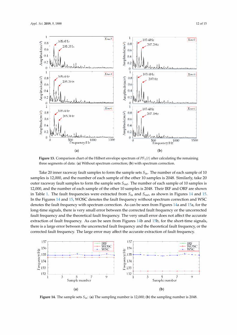
Appl. Sci. 2019, 9, 1888 12 of 15

Appl. Sci. 2019, 9, x FOR PEER REVIEW 12 of 16

(a) (b)

Figure 12. Comparison chart of the Hilbert envelope spectrum of 1( )PF t which is from Figure 10b: (a) Without spectrum correction; (b) with spectrum correction.

(a) (b)

Figure 13. Comparison chart of the Hilbert envelope spectrum of 1( )PF t after calculating the remaining three segments of data: (a) Without spectrum correction; (b) with spectrum correction.

Without spectrum correction, the fault frequency 105.6 Hz has a clear error according to the theoretical fault frequency 103.1 Hz, as shown in Figure 13a. That is because the frequency resolution wΔ is related to the sampling frequency sF and the sampling number N . The relationship between them is expressed by the formula of /sw F NΔ = . When the sampling frequency is constant, the frequency resolution wΔ is inversely proportional to the sampling number N . When the number of the four segments is 2048, the frequency resolution decreases and the spectrum is distorted. However, with spectrum correction, the fault frequency 103.4 Hz is almost equal to the theoretical fault frequency 103.1 Hz, as shown in Figure 13b. The spectrum correction

Figure 13. Comparison chart of the Hilbert envelope spectrum of PF1(t) after calculating the remainingthree segments of data: (a) Without spectrum correction; (b) with spectrum correction.

Take 20 inner raceway fault samples to form the sample sets Sin. The number of each sample of 10samples is 12,000, and the number of each sample of the other 10 samples is 2048. Similarly, take 20outer raceway fault samples to form the sample sets Sout. The number of each sample of 10 samples is12,000, and the number of each sample of the other 10 samples is 2048. Their IRF and ORF are shownin Table 1. The fault frequencies were extracted from Sin and Sout, as shown in Figures 14 and 15.In the Figures 14 and 15, WOSC denotes the fault frequency without spectrum correction and WSCdenotes the fault frequency with spectrum correction. As can be seen from Figures 14a and 15a, for thelong-time signals, there is very small error between the corrected fault frequency or the uncorrectedfault frequency and the theoretical fault frequency. The very small error does not affect the accurateextraction of fault frequency. As can be seen from Figures 14b and 15b, for the short-time signals,there is a large error between the uncorrected fault frequency and the theoretical fault frequency, or thecorrected fault frequency. The large error may affect the accurate extraction of fault frequency.

Appl. Sci. 2019, 9, x FOR PEER REVIEW 13 of 16

method can correct the spectral distortion of the short-time signals and restore the authenticity of the spectrum to some extent.

Take 20 inner raceway fault samples to form the sample sets inS . The number of each sample of 10 samples is 12,000, and the number of each sample of the other 10 samples is 2048. Similarly, take 20 outer raceway fault samples to form the sample sets outS . The number of each sample of 10 samples is 12,000, and the number of each sample of the other 10 samples is 2048. Their IRF and ORF are shown in Table 1. The fault frequencies were extracted from inS and outS , as shown in Figure 14 and Figure 15. In the Figure 14 and Figure 15, WOSC denotes the fault frequency without spectrum correction and WSC denotes the fault frequency with spectrum correction. As can be seen from Figures 14a and 15a, for the long-time signals, there is very small error between the corrected fault frequency or the uncorrected fault frequency and the theoretical fault frequency. The very small error does not affect the accurate extraction of fault frequency. As can be seen from Figures 14b and 15b, for the short-time signals, there is a large error between the uncorrected fault frequency and the theoretical fault frequency, or the corrected fault frequency. The large error may affect the accurate extraction of fault frequency.

(a) (b)

Figure 14. The sample sets inS : (a) The sampling number is 12,000; (b) the sampling number is 2048.

(a) (b)

Figure 15. The sample sets outS : (a) The sampling number is 12,000; (b) the sampling number is 2048.

4. Discussion

The fault signal of rolling bearing typically has non-stationary, nonlinear, and modulated characteristics. Compared with traditional signal processing technology, LMD can decompose signals self-adaptively on the basis of signals themselves. For the online real-time monitoring, it is an effective way to increase the diagnostic efficiency by reducing the sampling data while keeping the accuracy of fault frequency. For the long-time signals of rolling bearing, the fault frequency is almost equal to the theoretical fault frequency whether it is corrected or not. Therefore, it does not affect the extraction accuracy of fault frequency. However, for the short-time signals, the uncorrected fault

Figure 14. The sample sets Sin: (a) The sampling number is 12,000; (b) the sampling number is 2048.

Appl. Sci. 2019, 9, 1888 13 of 15

Appl. Sci. 2019, 9, x FOR PEER REVIEW 13 of 16

method can correct the spectral distortion of the short-time signals and restore the authenticity of the spectrum to some extent.

Take 20 inner raceway fault samples to form the sample sets inS . The number of each sample of 10 samples is 12,000, and the number of each sample of the other 10 samples is 2048. Similarly, take 20 outer raceway fault samples to form the sample sets outS . The number of each sample of 10 samples is 12,000, and the number of each sample of the other 10 samples is 2048. Their IRF and ORF are shown in Table 1. The fault frequencies were extracted from inS and outS , as shown in Figure 14 and Figure 15. In the Figure 14 and Figure 15, WOSC denotes the fault frequency without spectrum correction and WSC denotes the fault frequency with spectrum correction. As can be seen from Figures 14a and 15a, for the long-time signals, there is very small error between the corrected fault frequency or the uncorrected fault frequency and the theoretical fault frequency. The very small error does not affect the accurate extraction of fault frequency. As can be seen from Figures 14b and 15b, for the short-time signals, there is a large error between the uncorrected fault frequency and the theoretical fault frequency, or the corrected fault frequency. The large error may affect the accurate extraction of fault frequency.

(a) (b)

Figure 14. The sample sets inS : (a) The sampling number is 12,000; (b) the sampling number is 2048.

(a) (b)

Figure 15. The sample sets outS : (a) The sampling number is 12,000; (b) the sampling number is 2048.

4. Discussion

The fault signal of rolling bearing typically has non-stationary, nonlinear, and modulated characteristics. Compared with traditional signal processing technology, LMD can decompose signals self-adaptively on the basis of signals themselves. For the online real-time monitoring, it is an effective way to increase the diagnostic efficiency by reducing the sampling data while keeping the accuracy of fault frequency. For the long-time signals of rolling bearing, the fault frequency is almost equal to the theoretical fault frequency whether it is corrected or not. Therefore, it does not affect the extraction accuracy of fault frequency. However, for the short-time signals, the uncorrected fault

Figure 15. The sample sets Sout: (a) The sampling number is 12,000; (b) the sampling number is 2048.

4. Discussion

The fault signal of rolling bearing typically has non-stationary, nonlinear, and modulatedcharacteristics. Compared with traditional signal processing technology, LMD can decompose signalsself-adaptively on the basis of signals themselves. For the online real-time monitoring, it is an effectiveway to increase the diagnostic efficiency by reducing the sampling data while keeping the accuracy offault frequency. For the long-time signals of rolling bearing, the fault frequency is almost equal to thetheoretical fault frequency whether it is corrected or not. Therefore, it does not affect the extractionaccuracy of fault frequency. However, for the short-time signals, the uncorrected fault frequencyhas a certain error compared to the theoretical fault frequency. However, with spectrum correction,the fault frequency is basically equal to the theoretical fault frequency. It is shown that the proposedmethod of this paper is valid.

However, the proposed method of this paper has some shortcomings. How to properly determinethe sampling number of the short-time signals in the case of ensuring frequency accuracy andcomputational efficiency is a problem. It can be manually set according to the short-time signals itself.However, the signal is changing with the environment. If the sampling number does not change withthe change of the signal, it may lead to the mistakes of diagnosis, especially in the online real-timemonitoring. Another problem is how to completely eliminate the influence of the noise to the ratiocorrection method. The noise not only affects the direction of interpolation, but also affects the spectralaccuracy. How to avoid the interpolation in the opposite direction and get the determined correctionfrequency is another problem to be solved. Future research will focus on the further improvement ofthe algorithm and the coalescent of the proposed method of this paper and deep learning.

5. Conclusions

The fault diagnosis method which uses LMD and the ratio correction method is proposed forthe short-time signals of rolling bearing. The fault signal of rolling bearing at the inner raceway andthe outer raceway were analyzed by the proposed method. The results show that this method cangain a high frequency resolution, and extract the fault frequency accurately under the condition of theshort-time signals. Therefore, this method has a certain value of engineering applications. The proposedmethod of this paper can reduce the size of data samples while ensuring accuracy. The deep learningmodels can directly work on the raw data without any data preprocessing. Thus, it is worthwhile tomake further study of combining spectrum correction with the deep learning models for processing theshort-time signals. In earthquake engineering, many methods are utilized to solve problems related toearthquakes. For example, probabilistic risk-based performance evaluation of seismically was used toanalyze base-isolated steel structures under the influence of far-field earthquakes [38]. Besides, signalprocessing is one of the most typical applications in earthquake engineering. Seismic signals havethe characteristics of non-stationary and “short-time” random impulses. Thus, it is worthwhile tomake further study for handling the short-time signals of earthquake data by the proposed method ofthis paper.

Appl. Sci. 2019, 9, 1888 14 of 15

Author Contributions: Conceptualization, Y.D. and C.W.; methodology, Y.D.; software, Y.D. and C.W.; validation,Y.D. and C.W.; formal analysis, Y.D., C.W. and P.L.; investigation, Y.C.; resources, Y.C.; data curation, Y.D., C.W. andP.L.; writing—original draft preparation, Y.D.; writing—review and editing, Y.D., Y.C. and C.W.; visualization,C.W.; supervision, C.W.; project administration, C.W.; funding acquisition, C.W.

Funding: This research was funded by the National Key R & D Plan Program of China (2018YFB0106100),the Sichuan Science and Technology support Program (2019YFG0352, 2019YFG0098, 2017GZ0395 and 2017GZ0394).

Conflicts of Interest: The authors declare no conflict of interest.

References

1. Cohen, L. Time-frequency distributions-a review. Proc. IEEE 1989, 77, 941–981. [CrossRef]2. Mallat, S.G. A theory for multiresolution signal decomposition: The wavelet representation. IEEE Trans.

Patt. Anal. Mach. Intell. 1989, 11, 674–693. [CrossRef]3. Qin, S.R.; Zhong, Y.M. A new envelope algorithm of Hilbert–Huang Transform. Mech. Syst. Signal Pr. 2006,

20, 1941–1952. [CrossRef]4. Huang, N.E.; Wu, M.L.C.; Long, S.R.; Shen, S.S.P.; Qu, W.; Gloersen, P.; Fun, K.L. A confidence limit for the

empirical mode decomposition and Hilbert spectral analysis. Proc. A 2003, 459, 2317–2345. [CrossRef]5. Deng, Y.J.; Wang, W.; Qian, C.C.; Wang, Z.; Dai, D.J. Boundary-processing-technique in EMD method and

Hilbert transform. Chin. Sci. Bull. 2001, 46, 954. [CrossRef]6. Cheng, J.S.; Yu, D.J.; Yang, Y. Research on the intrinsic mode function (IMF) criterion in EMD method. Mech.

Syst. Signal Pr. 2006, 20, 817–824.7. Smith, J.S. The local mean decomposition and its application to EEG perception data. J. R. Soc. Interface 2005,

2, 443–454.8. Pan, H.; He, X.; Tang, S.; Meng, F. An improved bearing fault diagnosis method using one-dimensional CNN

and LSTM. J. Mech. Eng. 2018, 64, 443–452.9. Jing, L.; Zhao, P.; Li, P.; Xu, X. A convolutional neural network based feature learning and fault diagnosis

method for the condition monitoring of gearbox. Measurement 2017, 111, 1–10. [CrossRef]10. Yang, Y.; Liao, Y.; Meng, G.; Lee, J. A hybrid feature selection scheme for unsupervised learning and its

application in bearing fault diagnosis. Expert Syst. Appl. 2011, 38, 11311–11320. [CrossRef]11. Cheng, J.S.; Zhang, H.; Yang, Y. A comparative study of local mean decomposition and empirical mode

decomposition. J. Vibr. Shock 2009, 28, 13–16.12. Zhang, F.S.; Geng, Z.X.; Yuan, W. The algorithm of interpolating windowed FFT for harmonic analysis of

electric power system. IEEE Trans. Power Deliv. 2001, 16, 160–164. [CrossRef]13. Luo, J.F.; Xie, M. Phase difference methods based on asymmetric windows. Mech. Syst. Signal Process. 2015,

54, 52–67. [CrossRef]14. Duan, H.M.; Qin, S.R.; Li, N. Review of correction methods for discrete spectrum. J. Vibr. Shock 2007, 26,

138–145.15. Xie, M.; Ding, K. A new correction method for discrete spectrum analysis. J. Chongqing Univ. Nat. Sci. Ed.

1995, 18, 48–54.16. Grandke, T. Interpolation algorithms for discrete Fourier transforms of weighted signals. IEEE Trans. Instrum.

Meas. 1983, 32, 350–355. [CrossRef]17. Ding, K.; Jiang, L.Q. Energy centrobaric correction method for discrete spectrum. J. Vibr. Eng. 2001, 14,

354–358.18. Lin, H.B.; Ding, K. Energy based signal parameter estimation method and a comparative study of different

frequency estimators. Mech. Syst. Signal Process. 2011, 25, 452–464.19. Belega, D.; Dallet, D.; Petri, D. Accuracy of the normalized frequency estimation of a discrete-time sine-wave

by the energy-based method. IEEE Trans. Instrum. Meas. 2012, 61, 111–121. [CrossRef]20. Candan, C. A method for fine resolution frequency estimation from three DFT samples. Signal Process. Lett.

IEEE 2011, 18, 351–354. [CrossRef]21. Abatzoglou, T.; Candan, C. Analysis and further improvement of fine resolution frequency estimation

method from three DFT samples. Signal Process. Lett. IEEE 2013, 20, 913–916.22. Macleod, M.D. Fast nearly ML estimation of the parameters of real or complex single tones or resolved

multiple tones. IEEE Trans. Signal Process. 1998, 46, 141–148. [CrossRef]

Appl. Sci. 2019, 9, 1888 15 of 15

23. Jacobsen, E.; Kootsookos, P. Fast, accurate frequency estimators. Signal Process. Magaz. IEEE 2007, 24,123–125. [CrossRef]

24. Calro, O.; Diaro, P. The influence of windowing on the accuracy of multifrequency signal parameter estimation.IEEE Trans. Instrum. Meas. 1992, 41, 256–261.

25. Schoukens, J.; Pintelon, R.; Van, H.H. The interpolated fast Fourier transform: A comparative study. IEEETrans. Instrum. Meas. 1991, 41, 226–232. [CrossRef]

26. Xie, M.; Ding, K. Corrections for frequency, amplitude and phase in a fast Fourier transform of a harmonicsignal. Mech. Syst. Signal Process. 1996, 10, 211–221.

27. Dishan, H. Phase error in fast Fourier transform analysis. Mech. Syst. Signal Process. 1995, 9, 113–118.[CrossRef]

28. Xie, M.; Ding, K. Correction method of spectrum analysis. J. Vibr. Eng. 1994, 7, 172–179.29. Ding, K.; Xie, M. Method of improving the speed and accuracy of FFT and spectral analysis. J. Chongqing

Univ. Nat. Sci. Ed. 1992, 15, 51–57.30. Zhang, Y.; Qin, Y.; Xing, Z.Y.; Jia, L.M.; Cheng, X.Q. Roller bearing safety region estimation and state

identification based on LMD–PCA–LSSVM. Measurement 2013, 46, 1315–1324. [CrossRef]31. Ren, D.Q.; Yang, S.X.; Wu, Z.T.; Yan, G.B. Research on end effect of LMD based time-frequency analysis in

rotating machinery fault diagnosis. China Mech. Eng. 2012, 23, 951–956.32. Wang, L.; Liu, Z.; Miao, Q. Time-Frequency analysis based on ensemble local mean decomposition and fast

kurtogram for rotating machinery fault diagnosis. Mech. Syst. Signal Process. 2018, 103, 60–75. [CrossRef]33. Liu, Z.L.; Zuo, M.J.; Jin, Y.Q.; Pan, D.; Qin, Y. Improved local mean decomposition for modulation information

mining and its application to machinery fault diagnosis. J. Sound Vibr. 2017, 397, 266–281. [CrossRef]34. Case Western Reserve University Bearing Data Center. Available online: http://csegroups.case.edu/

bearingdatacenter/home (accessed on 18 October 2018).35. Rife, D.; Boorstyn, R. Single tone parameter estimation from discrete-time observations. IEEE Trans. Inf.

Theory 1974, 20, 591–598. [CrossRef]36. Xu, C.Y.; Ding, K.; Lin, H.B. Noise influence on amplitude and phase estimation accuracy by interpolation

method for discrete spectrum. J. Vibr. Eng. 2011, 24, 633–638.37. Chen, K.F.; Jiang, J.T.; Crowsen, S. Against the long-range spectral leakage of the cosine window family.

Comput. Phys. Commun. 2009, 180, 904–911. [CrossRef]38. Aryan, R.R.; Mehdi, B. Probabilistic Risk-Based Performance Evaluation of Seismically Base-Isolated Steel

Structures Subjected to Far-Field Earthquakes. Buildings 2018, 8, 128.

© 2019 by the authors. Licensee MDPI, Basel, Switzerland. This article is an open accessarticle distributed under the terms and conditions of the Creative Commons Attribution(CC BY) license (http://creativecommons.org/licenses/by/4.0/).