improving the spatial accuracy of digital maps
TRANSCRIPT


Improving the Spatial Accuracy of Digital Maps: An Algorithm to Align the Road Network to Real GPS Data
Rachel Blair
Professor Alain L. Kornhauser
17 April 2006
Submitted in partial fulfillment of the requirements for the degree of Bachelor of Science in Engineering
Department of Operations Research and Financial Engineering Princeton University

I hereby declare that I am the sole author of this thesis. I authorize Princeton University to lend this thesis to other institutions or individuals for the purpose of scholarly research. ________________ Rachel M Blair I further authorize Princeton University to reproduce this thesis by photocopying or by other means, in total or in part, at the request of other institutions or individuals for the purpose of scholarly research. ________________ Rachel M Blair

Acknowledgements I would like to thank Professor Kornhauser for his guidance and support through my entire Princeton career and in preparing this thesis. He has been a wonderful teacher and mentor. I would also like to thank TravRoute and ALK Technologies for their technical support and for allowing me to use their data and their program, CoPilot, to create this thesis. The ORFE Department and all of its administrators were extremely helpful in the process of writing and developing. I thank them for their coordination.
A special thanks is due to my good friend, Andreanne Morin. I am grateful the support she gave me while finishing this thesis. She has helped make this year one of my best years at Princeton. I would not have made it without her.
To my parents I would like to express my utmost gratitude, respect, and love.
Thanks you for the emotional and financial support in finishing this thesis and in making it through Princeton thus far. They are the two most loving people I know, and I count my lucky stars to have them as parents.

Abstract The objective of this thesis is to evaluate how to use algorithmic methods to update
digital map networks. Manually editing large amounts of data is tedious and
cumbersome. Creating an automatic component of the editing process can greatly
reduce the cost of the editing process. This thesis will apply this principle to create
an improved method for updating digital map networks using real GPS data. Given
a set of real GPS data corresponding to a selected route, algorithmically moving the
nodes and links that form a given route would be more efficient than manual moving
each link and node. The task will be divided into two steps. First, the route will be
selected by the editor by examining the GPS data available. After selecting a route,
the nodes, links, shape points of that section of network will be repositioned to more
closely align with the GPS points

Table of Contents
Chapter 1: Introduction 1
1.1 GPS and Digital Maps
1.2 Motivation for this Thesis
1.3 Objective of this Thesis
1.4 Scope of this Thesis
1.5 Organization of this Thesis
Chapter 2: The GPS Set and CoPilot Digital Maps 10
2.1 The Evolution of Digital Maps
2.2 The CoPilot Program
2.3 The Map Matching Process:
2.4 Snap Values
2.5 The CoPilot Editor
2.6 Error Associated with Global Positioning Systems
Chapter 3: Route Selection and Simple Route Alignment 20
3.1 Route Selection
3.2 Nodes with Two Emanating Links
3.3 Data Collection
3.4 Repositioning the Node
3.5 Implementation of the Simple Route Algorithm
3.6 Performance of the Algorithm
Chapter 4: Node Alignment at Branched Intersections 32
4.1 Theory
4.2 Data Collection: Estimating Sufficient Data Ranges
4.3 Median Heading: the Slope of a Linear Equation

4.4 Creating Separate Data Sets: ggdA and ggdB
4.5 Regression of GPS Data Sets to find a Y-Intercept
4.6 Locating (X0,Yo): Longitude and Latitude of the Node
Chapter 5: Shapepoints 47
5.1 Determining Where Shapepoints are Needed
5.2 Binary Approach to the Addition of Shapepoints
5.3 Greatest Deviation Approach to the Addition of Shapepoints
Chapter 6: Conclusion 56
6.1 Implications
6.2 Strengths and Weaknesses
6.3 Future Research
Works Cited and Referenced 60
Appendix A: Code for Simple Route Alignment 62 Appendix B: Code for Intersection Alignment 68 Appendix C: Structure of the Algorithm 73

- 1 -
Chapter 1: Introduction
The use of digital maps has increased dramatically over the past decade with
the use of computer routing programs and in-car navigations systems. Digital maps
recreate the spatial characteristics of a road network in a computer program and
store important information about the types of roads, directions of travel, and any
special restrictions or attractions associated with certain routes. There are many
advantages to using digital maps rather than traditional paper maps. Storing
information using paper maps quickly becomes cumbersome with an area larger
than a county. Digital Maps allow the user to access only the areas of interest
without having to sort through extraneous information. The area covered in one
screen and the level of detail can be adjusted to suite the needs of the user. Also
the fast pace of urban growth can be better maintained in digital format. Roads are
constantly being added and changed as development in both urban and rural areas
grows. Digital maps can be easily updated to accommodate such changes. The
most common use of digital maps is for creating point to point directions. Websites
such as MapQuest.com and Maps.Google.com use preferences such as avoiding
interstate highways to give the user personalized directions. They can also be used

- 2 -
to pinpoint amenities along the way: gas stations, restaurants, and other points of
interest. The use of vehicle navigation systems has increased the need for reliable
digital maps. They are a crucial element of all navigations systems; however, digital
maps are still in many places inaccurate and incomplete. The statistical and
positional accuracy needs to be improved for the performance of navigation
programs to improve. This thesis proposes a way to improve the positional accuracy
of sections of digital maps using data from vehicles traveling on the road network.
1.1 GPS and Digital Maps
The coordinate system which digital maps use corresponds to the GPS
position of the roads and intersections in space. Global Positioning Systems (GPS)
consist of satellites orbiting the earth and their corresponding receivers on the earth.
The GPS satellites transmit digital signals which contain data including distance and
travel time to the receiver on earth. Based on the information the GPS receivers
gather from four satellites in orbit it pinpoints its exact location on the surface of the
earth and the velocity of travel at any given time. Each GPS point, therefore, has a
time, latitude, longitude, and velocity. These GPS points provide a framework in
which to organize the digital maps.
Roads of all types are represented in the digital maps by a set of links. Each
link has one node at each end and a given number of shapepoints to represent any
curvature in the road. A node is situated on a digital map according to a longitude
and latitude. The nodes act as anchors to the link and the shapepoints are placed in
between the nodes to break the link into piecewise linear segments. Shapepoints
create the effect of curvature depending on the frequency and location of the points
and also have positional values of longitude and latitude. These nodes and
shapepoints in the X/Y plane compose the spatial design of the digital road map.

- 3 -
Figure 1.1 demonstrates the spatial attributes of the nodes and shapepoints. The
green squares are the nodes and the blue circles are the shapepoints. The red lines
show the same set of links after the nodes have been moved closer to the GPS data
shapepoints added to fit the curvature of the data between the nodes. This thesis
will examine a small set of links similar to those in Figure 1.1 to edit their location in
space based on real GPS data.
An important application of GPS and digital maps is real time navigation
assistance. CoPilot, developed by ALK Technologies Inc., is a navigation software
which uses a GPS receiver in the vehicle to provide real time driving directions to a
destination which the user programs. The GPS receiver sends a longitude and
latitude that is plotted on the digital map, displaying the location of the vehicle on the
map in real time. The CoPilot program plots the GPS position of the vehicle. This
continuous stream of GPS data allows the program to provide updated directions
and travel information. The program can be set to record the user’s GPS tracks. A
GPS track is the position of the vehicle in terms of longitude and latitude and a
direction of travel as well as the speed of the vehicle and the time of travel. This is
the data this thesis will use to adjust the spatial characteristics of a digital road map.
Figure 1.1 also displays the GPS tracks of two vehicles traveling on a road. The
tracks are located slightly below the road, although the program recognizes which
road it is traveling on because of their proximity to the route.

- 4 -
Figure 1.1: Map Alignment The green squares and blue circles represent the original nodes and shapepoints
corresponding to the original set of links. The red route shows a better spatial position of the nodes and shapepoints to align with the GPS tracks. Downward
pointing arrows correspond to the new location of nodes and upward pointing arrows correspond to the location of new shapepoints.
1.2 Motivation for this thesis
The spatial position of nodes and links which make up the digital road
network are often not in the correct location as shown in Figure 1.1. Often the digital
map road segments are close enough to their real location in space that the program
can determine which road the vehicle is on, but it is important for a variety of reason
that the nodes and links which represent the road be moved to the exact location in
space where the GPS tracks are recorded. Another concern is that the spatial
characteristics of roads change; new roads are added and construction moves roads
and intersections to a different location in space. The roadway network is a system
which is constantly updated and altered. Construction and development in urban
areas can be difficult to keep pace with. Updating digital maps is a necessary and
also time-consuming task. Also, since digital maps use linear segments to represent

- 5 -
curved roads, often the road segments deviate significantly from the true nature of
the road. In order to find these deviations of the digital map from the road network,
the GPS tracks from the vehicles using a GPS navigation system are plotted on the
digital map. The more vehicles travel on a given route collecting information, the
more data which is available to compare to the position and shape of the links which
make up that route. Plotting multiple tracks on the map creates a clearer picture of
where the roads and the data do not align properly. Figure 1.2 shows a section of
digital map where the GPS points deviate from the road. The nodes and links can
be moved closer to the GPS tracks gathered from traveling on that road. In this
figure the road needs to be shifted in down toward the GPS points. In other cases
where map alignment is needed, the shapepoints do not align properly with the
curvature of the road and need to be added. Shapepoints can easily be added or
subtracted to change any link which veers away from the data in between links. The
GPS tracks which align over a set of links verify the correct position in space of a
road. Also, it is possible to have tracks with no links associated with them,
suggesting the presence of a missing road from the network.

- 6 -
Figure 1.2 (a)
Figure 1.2 (b)
Figure 1.2: Example of alignment of a digital map to GPS tracks The small squares with dashes are the GPS tracks. The vehicle is traveling in the
direction of the dash. (a) This map shows the GPS tracks plotted on the digital map as collected. (b) The nodes and links have been adjusted to align the road segments
with the GPS tracks. Another way of determining whether the digital map contains the correct
spatial alignment can be done by physically surveying the area or by using aerial
photography to find the correct position and characteristics of roads. These are
valuable methods for verifying the accuracy of digital maps; however, they are costly
and cumbersome. When a sufficient amount of GPS data is available, it can save
time and money to use the data to correct digital maps. The GPS receiver in
vehicles with navigation systems sends the data to the main program where it is
recorded. This set of GPS tracks can be downloaded to a computer and compiled to
create aggregate data set of GPS tracks. These data sets exist and can be
collected for use in projects such as this thesis. A large enough set of GPS data
- 7 -
provides substantial evidence of where the locations of roads are in space. If the
links making up the road in the digital map do not match the GPS tracks, they can be
manually moved to more closely align with the data. However, an algorithm could
also be used to align the links with the GPS data more easily than moving nodes and
shapepoints manually.
1.3 Objective of this thesis
Adjusting the spatial attributes of a roadway is an important part of keeping
digital maps accurate and up to date. In addition to the changes which occur over
time much of the existing digital map was originally positioned using inaccurate data.
The road network was created in a digital map using sources including census data
which have a significant amount of error. The roads are often located a set distance
away from where it is located on the map. The roadway network is a system that is
also continually being altered, so the digital map needs to be able to be edited in a
timely and manageable way. It is important to make digital maps more accurate.
The user of digital maps is able zoom to any location at a high level of detail. This,
however, does not mean that the map is spatially accurate. Using the positions of
GPS tracks collected from vehicles which have recently traveled the roadway
network provide a more accurate and recent source of information. An algorithm
could adjust the nodes, links, and shapepoints which make up the spatial position of
the roads to better align with the collection of GPS tracks.
This thesis will develop an algorithm which adjusts a small segment of
roadway to better align with the GPS tracks associated that particular route. The
basic problem is how to spatially modify a selected section of links and nodes to
more accurately reflect the true nature of the road. The thesis assumes a sufficient
amount of GPS data, where available, accurately reflects the location and shape of

- 8 -
the roads in the network. Both the position of the nodes and the curvature of the
road can be algorithmically aligned with GPS points near the section of road.
Therefore the thesis aims to create an algorithm which more accurately aligns the
position of nodes and links with the corresponding GPS data.
1.4 Scope of the Thesis
The algorithm will preserve the basic properties of the link; only the spatial
characteristics will be altered. Link properties contain important information about
the type of road, any restrictions it might have. It is important to keep this travel
information in tact in the network. The algorithm will also not attempt to add new
links or nodes, only the number of shapepoints used will change based on the
curvature of the road. This means that it will not attempt to create new sections of
roads. It is not uncommon for an entire road to be missing from the network or for a
new road or subdivision to have been added since the digital map was last updated.
Since the algorithm is confined to spatial alignment and does not add new links or
nodes it will be impossible to address of the problem of missing or new roads.
The algorithm is implemented only after the user has selected a given route
to be edited. Since it will deal with a small section of road at a time on one specific
route, the algorithm will not change the representation of direction in the road. A one-
way road will keep it’s orientation in the same direction and a two-way road will not
be changed. The two-way directionality is always assumed to be correct even if the
only data available is from one direction of travel. In this case the algorithm will
attempt to align the road to a probable centerline. In some cases highways are split
into two roads with one way travel located in different places and often curving
differently than the opposing side. The algorithm presented in this thesis will always
preserve the original two-way or one-way property of the links.

- 9 -
1.5 Organization of the Thesis
The goal of this thesis is to create an algorithm that will align a set of nodes
and links representing a section of road network more precisely to its corresponding
GPS tracks. The reliability of the GPS data is an important consideration in this
thesis since the algorithm’s only source for spatial alignment is the GPS points.
Therefore, it will be important to cover the errors associated with GPS and how that
could affect the results of this alignment process. The development of the algorithm
will begin with the simplest possible case of alignment and then add increasing
complexity. The first step is to consider the spatial position of the nodes and the next
step is to place shapepoints on the links to create curvature in the road. After the
basic alignment problem has been addressed, then the problem of branch links from
the selected route will be considered. One of the major challenges is to limit the
change of the surrounding network when moving the nodes and links of the section
of roadway to be edited. Finally this thesis will explore the impact of this algorithm
on the uses of digital maps. Making the road network more accurate is an important
first step in new applications for digital maps.

- 10 -
Chapter 2: The GPS Data Set and CoPilot Digital Maps
This chapter will explore the history of digital maps and ways which have
been implemented to improve their accuracy. This thesis uses a specific digital map
program to develop an algorithm to adjust the spatial characteristics of the map. The
algorithm can however be modified for use on other digital map programs by
adapting the code to fit the needs of another software. CoPilot has a set of unique
processes and terminology which will be explored in this chapter to give the reader a
better understanding of how the algorithm is developed. The GPS data set as well
has properties which are relevant to how the algorithm is developed and will be
looked at in this chapter.
2.1 The Evolution of Digital Maps
Most digital maps have been developed using a database created by the U.S.
Geological Survey and the Census Bureau. The data, labeled TIGER, is a
topographically integrated geographic encoding and referencing system. The data
was originally created by scanning US Geological Survey (USGS) topographic maps

- 11 -
and searching for significant structures.1 The topographic maps provided locations
of major roads, railroads, and terrain features which were then scanned into a digital
file. The maps were on a 1:100,000 scale. These maps were sufficient for rural
areas but were not able to handle the detail necessary for cities and other tightly
developed urban areas. For these urban areas the Census Bureau used GBF/
DIME files created in 1967 in preparation for the 1970 census. The acronym DIME
stands for “Dual Independent Map Encoding” which was an important technical
breakthrough in creating digital maps. DIME is a method used to collect data to
encode map features in data files.2 These files do not contain address ranges or
other statistical information rather contains the structural features of urban
environments. The GBF/DIME files constituted only 2% of the original TIGER
database created in the 1970.3 Throughout the 1970’s GBF/DIME files were made
into digital format for all US cities and were integrated into the TIGER system as
data became available.4 The TIGER database is continually updated as new
information becomes available from work done by the Department of Commerce and
the Census Bureau and from local government providing statistical and geographical
information.
The TIGER database, while the most comprehensive file for digital road
maps, still lacks positional accuracy in many locations and is still missing roads and
new developments. In 2002 the US Census Bureau commissioned a private
corporation for the TIGER Accuracy Improvement Project. The Harris Corporation
1 US Census Bureau, TIGER/MAF , <www.census.gov/geo/www/tiger/> 2 U.S. Department of Commerce, U.S. Census Bureau, Geographic Base File/Dual Independent Map Encoding (GBF/DIME), 1980 Description, ICPSR 3 Tiger Database FAQ <www.census.gov/cgi-bin/geo/tigerfaq> “Where did the data come from that is used in the TIGER Map Service?” 4 “The Story of DIME: A Progress Report,” The GIS History Project

- 12 -
was delegated the responsibility of creating a complete and current list of address for
both residential and business.5 This goal of this project, however, was to improve
statistical accuracy, not positional accuracy. The U.S. Census Bureau TIGER
website states:
TIGER was never designed (or funded) to be a high precision network because we don’t need such precision and it was compiled from a variety of sources…We felt that potential distortions introduced were not enough to cause problems for our uses of the data so we did not expand resources to reconcile them…We recognize the limitations of TIGER data for high precision users. It was also done before the widespread public use of GPS technology. Not many people inside or outside of the Census Bureau anticipated the scale or impact of TIGER to applications beyond the Census.6
The TIGER data was not originally designed for high precision use, which is needed
for accurate GPS navigation. This database has become the foundation of digital
maps for GPS navigations systems. As the use of the data for this purpose has
increased, the need for positional accuracy and precision in the data has also
increased. Each new release of the TIGER data provides increasing accuracy and
completeness; however it is not enough to keep pace with the demand for accurate
digital maps by GPS navigation developers and users.
Research using GPS data to realign digital maps is limited and done primarily
by the private sector. Much of the work using real GPS data has been to estimate
travel times. The DaimlerChrysler Research and Technology Center sponsored a
project to improve digital road maps and gain an understanding of driving behavior
and estimated travel times. Rogers, Schroedl, and Handley studied GPS vehicle
tracks to create estimates for road information, such as location of the centerline and
5 GCSD Press Release, “Harris Corporation Awarded $200 Million Contract for U.S. Census Bureau’s MAP/TIGER Accuracy Improvement Project,” June 25, 2002. 6 Cartography and Geographic Information Systems, Government Information Quarterly, Vol 17. NO 1, 1990

- 13 -
number of lanes on the road.7 The use of GPS tracks from vehicles to gather
information on traffic patterns and individual driving habits is another area of
research in the private industry.8 Schroedl et al. also working for DaimlerChrylser
Research and Technology Center conducted a broad study to determine the
feasibility of using real GPS data to extract results about vehicle transportation. This
thesis uses real GPS data to improve the positional accuracy of the digital road.
2.2 The CoPilot Program
ALK Technologies Inc. developed a series of digital map programs named
CoPilot. The CoPilot software has been designed for use in laptop computers,
Pocket PC’s, and cellular telephones. The specific product used in developing this
thesis concerns the digital map program which is designed to run on a PC. Real
time navigational assistance comes from the handheld unit and GPS receiver which
is placed in the vehicle. The device gives verbal directions to the driver and plots the
vehicle’s current location on the map. Every three seconds the exact GPS point
from the receiver is processed and recorded by the program. The GPS points from
travel along the road networks are called ‘tracks.’ The tracks from an individual unit
can be downloaded to a PC and plotted on the digital map to show the driver where
he or she has traveled. CoPilot users have voluntarily submitted these GPS tracks
to ALK Technologies. ALK Technologies has acquired an extensive amount of data
from CoPilot customers. These tracks are valuable for the task of increasing the
accuracy of digital maps, by fixing roads that are not accurately located and adding
7 Rogers, S., Langley, P., & Wilson, C. “Learning to predict lane occupancy using GPS and digital maps.” Proceedings of the Fifth International Conference on Knowledge Discovery and Data Mining. San Diego, CA: ACM Press, 1999. 8 Schroedl, S., Wagstaff, K., Rogers, S., Langley, P., & Wilson, C. Mining GPS traces for map refinement. Knowledge Discovery and Data Mining, 2004

- 14 -
new roads. This thesis will use a subset of the GPS tracks acquired from ALK
Technologies for data in order to better align sections of the digital map.
2.3 The Map Matching Process
In order to use a real time navigational system, such as CoPilot, the program
must be able to match the data collected from the GPS receiver with the road the
user is traveling in. Since the road is not always located exactly at the latitude and
longitude the GPS receiver reports due to GPS error or a misplaced set of links on
the digital map, the program has an algorithm designed to match the GPS point to a
specific road link. Copilot uses an algorithm that weights direction as well as the
position of the vehicle in order to place the vehicle on the road which it is most likely
traveling. The most likely road match has both a parallel direction to the GPS track
and has the closest distance from road to track. After matching the GPS point to the
road link the direction and the position are plotted on the map. This algorithm will be
an important part of the alignment of the links to the data.
2.4 Snap Values
Snap values are an important tool in the algorithm used in this thesis. When
a car travels with an active CoPilot navigational device, the GPS receiver is
constantly sends a position (latitude, longitude) to the device. The CoPilot program
matches the GPS tracks to the road which it thinks the car is most likely traveling.
The result of going through the map-matching process is called “snapping.” After a
GPS track is snapped to a link the program can locate where the vehicle is in the
road network to continue the navigational assistance. Each GPS track is assigned a
set of values when it is snapped to the map. Snap values include the date and time
of travel. The most important snap values for the purpose of this thesis are the
latitude and longitude, the heading, the snap link, the snap percentage, and the snap
- 15 -
weight. The snap link is the link which CoPilot identifies as the link in the road
network which the car is traveling on. The snap percentage gives an exact location
on the link where the car is traveling in terms of a percentage from the A node to the
B node. Finally the snap weight is a number between 0.00 and 1.00 which measure
the “goodness” of the fit. Snap values closer to 1.00 means the likelihood is high
that the car is actually traveling on the road CoPilot snapped it to.
2.5 The CoPilot Editor
The editor is the software also developed by ALK Technologies which also
ALK employees to edit the digital road map network. All of the information that is
stored in the road map available in the CoPilot program is edited in this program.
Map features, specifically road features are changed or created by changing the
properties of the individual links which make up a road. For example, link properties
include important information such as what type of road the link represents, any
restrictions the road has, and any address ranges which are associated with that
link. In addition to changing physical properties of links the editor program contains
tools to adjust the spatial characteristics of the digital road map. The editor can
create nodes as well as move them. Intersection can be moved as well as broken
up into via-ducting roads. Features such as no left turn restrictions are also added.
Links can be straightened and shapepoints re-added at the desired locations on the
link to simulate curvature. The algorithm presented in the thesis will be an addition
to the editor software. A separate mode is added to the CoPilot editor. Entering this
mode will call the “Move_Link_to_GPS” function which will execute the adjustment of
the spatial characteristics of the highlighted route. This function manipulates some
of the features of the CoPilot editor such as the movement of nodes, straightening of
and adding shapepoints to the links.

- 16 -
2.6 Error associated with Global Positioning Systems
GPS data has inherent error. Different receivers report different coordinates
for the same position in space. There are many reasons for this including receiver
malfunction, satellite clock error, satellite orbit error, or troposphere error9. Whatever
the cause of the error, it is important for the navigation program to be able to adapt
to a reasonable margin of error. As a result of the margin of error, when the GPS
tracks are plotted in two-dimensional space on the digital map, there is a spread of
tracks. Usually the tracks are close enough together so that just by observation it is
easy to tell that the tracks are from vehicles traveling on the same road. Sometimes
one track of GPS points is far off from the tracks corresponding to a given road. This
is usually the sign of a faulty GPS receiver causing bad GPS data. It is important to
remove the bad data from the map before running the algorithm to correct spatial
characteristics. Each set of tracks in the data has a unique identification. As a
CoPilot customers drive in their cars and GPS tracks are collected, the tracks from
one trip from start to finish are bundled into one data structure with a trip
identification number. From the time CoPilot starts navigating to an intermediate or
final destination where the car is turned off the GPS tracks are collected into one trip.
It is possible to differentiate between trips by checking the trip ID on the GPS track
properties. When a specific data track is an outlier, lying further outside of the
majority of the data, it is possible in the CoPilot editor to remove the entire string of
GPS tracks which make up that particular trip. By visually examining the data before
the algorithm is executed bad GPS data can be removed.
9 “Error analysis of GPS point positioning,” National Geodetic Survey, http://www.ngs.noaa.gov/FGCS/info/sans_SA/docs/p-error.htm

- 17 -
Figure 2.1: Highland Village, TX
The GPS tracks displayed in grey are the points with a snap value greater
than or equal to 0.8. The closer to 1.0 the snap value is, the more confident the
CoPilot program is that the car is indeed on the road to which it has been map-
matched. GPS tracks with a blue color have a snap values less than 0.8 and GPS
tracks that are highlighted red have snap values less than 0.5. Most of the tracks
are grey along Legacy Drive but there is one string of GPS tracks located above the
bulk of the GPS tracks. This set of tracks for the purposes of this study is
considered bad data. The tracks are not smooth representing the motion of a curve
and lie outside of a significant amount of data. These points have that have snap
values less than 0.8 can be discarded; however, there are other points which also
have similar snap values. The blue points at the bottom of the curve are valuable
data for correcting the spatial characteristics of this link. A shapepoint is needed to
add more curvature to the road and bring the link closer to the GPS points. After re-

- 18 -
snapping the values GPS points to the link on Legacy Dr. the average snap value of
the set of points which were blue was raised from 0.74 to 0.85. This is a significant
improvement. At the bottom of Figure 2.1 the GPS tracks turn red where Corporate
Dr. ends on the map and CoPilot has no road to match the GPS signal to. It is
probable that Corporate Drive continues but is misrepresented on the CoPilot map.
This, however, is not the focus of this thesis, but it is important to recognize what
types of data will work for this project. GPS data will snap values of less than 0.5 will
not work with this algorithm because they are not map-matched to a specific road
and the algorithm does not add new roads or links.
According to the Federal Aviation Administration most GPS receivers are
accurate to within 10 meters10. The inherent error is GPS signals causes variance in
the latitude and longitude of cars traveling on the same road. The following is a
distribution of the GPS tracks gathered along I-35 (Figure 2.2a). There is one set of
GPS tracks which is clearly separate from the majority of the data and can be
considered an outlier. The highway is oriented north/south so the majority of the
GPS tracks have a heading of 0 for north-bound travel and 180 for south bound
travel. The latitude of the GPS tracks will change based on the position on the link,
but the longitude should remain roughly constant. The variance of the longitude is
an indicator of the error inherent in GPS receivers.
10 Federal Aviation Administration, Satellite Navigation Product Teams, < http://www.gps.faa.gov>

- 19 -
a) b)
Distribution of GPS Longitude on North South Highway
0
100200
300400
500
-9731
7958
-973
1785
0.39
-973
17742
.78
-973
1763
5.17
-973
1752
7.56
-973
1741
9.95
-9731
7312
.34
-9731
7204
.73
-973
1709
7.12
LatitudeF
requ
ency
c)
Distibution of GPS Longitude on a North South Highway
050
100150200250300
-9731
7411
-973
1737
8.08
-973
1734
5.17
-973
1731
2.25
-973
17279
.33
-973
17246
.42
-973
1721
3.5
-973
1718
0.58
-973
1714
7.67
-973
1711
4.75
-973
1708
1.83
-973
1704
8.92More
Latitude
Fre
que
ncy
Figure 2.2 Histogram of GPS Longitude on a N-S Highway (I-35)
The distribution is skewed heavily to the left because of the outlier in the GPS data (b). Removing this set of GPS tracks from the data produces a more regular distribution (c). The histogram of the data creates a rough bell shaped curve for each direction of travel. Different GPS receivers will give slightly different reading for the same location in space.

- 20 -
Chapter 3: Route Selection and Simple Route Alignment
This thesis will start with the simplest case of algorithmic alignment of digital
roads to GPS data and add complexity in progressive steps. The simplest case is a
straight route with no major curve or branched intersection. This means that the
nodes in the selected links act more as shapepoints and do not represent
intersections. This is a common situation in places where the map is representing a
long stretch of road with no intersections. The nodes which connect the road
segments need to be moved the center of the corresponding GPS data. The basic
problem is how to adjust the spatial position of a chain of n links and n+1 connecting
nodes in order to better align with the set of GPS points associated with the selected
linear links.
3.1 Route Selection
A special mode in the CoPilot editor is created for the purpose of this
algorithm. If more than one link is selected the algorithm will commence. The
selected route should be one which the user can see from beginning to end. Bad
data must first be removed before starting the alignment process or the results could
be skewed. Also the beginning and end of the route should be noted in case
adjustments need to be made at the end nodes.

- 21 -
3.2 Nodes with Two Emanating Arcs Containing Data
One instance of this alignment process is a straight road with a node
anchoring two links which form the same road. In this case the node acts the same
way as a shapepoint. Breaking one long link down into smaller links makes the data
more manageable. Link properties such as address ranges, will be more spatially
accurate the shorter the links are. The algorithm presented will not break up a link by
adding or subtracting nodes rather move them to a more accurate location. Moving
the nodes will change the length of the link; however the distance is not significant to
change any link properties, such as addresses. The other instance of this situation
is a node which anchors three or four links but only two links from the same road
have data. Figure 3.1 shows a route which can be adjusted using the simple route
alignment method. Nodes 1, 2, and 5 are links with three incoming links, but only
have data on two links. Nodes 3, 4, 6, and 7 are nodes with only two incoming links
and will also be adjusted to fit the GPS tracks more closely. This algorithm will align
these intersection nodes the same way as nodes with two emanating links. The
latitude and longitude associated with each node needs to reassigned based on the
average latitude and longitude of the closest GPS data. It is also important to be
aware of the surrounding network and make sure that the selected route which is to
be aligned does not become disconnected from or disturb significantly the
surrounding area. The first node and last node of the selected route will not be
adjusted by the algorithm and thus must be manually edited. This can be done with
little extra effort after the selected nodes have been moved to a new location.

- 22 -
Figure 3.1: Nodes 1 through 7 will be aligned to the GPS tracks using the simple route alignment method. 3.3 Gathering Data
The latitude and longitude of the node needs to be reassigned. It needs to
the most accurate location provided by the GPS data associated with the node. One
difficulty is deciding how to gather data around the node. The map-matching
algorithm assigns the GPS tracks to the original road link, but not to a given node.
The challenge is to find the appropriate data set to use to change the spatial position
of the node. If this part of the algorithm is implemented, there are two links
containing data for each node in the route. The algorithm will collect data from a
given radius around each node. The radius varies depending on the type of road.
CoPilot has 8 classes of roads which are mapped: interstate highways, interstate
highways with no ramps, divided highways, primary roads, ferries, secondary roads,
ramps, and local roads. This thesis will address spatial alignment of interstate
highways (Class 1), divided highways (Class 3), primary roads (Class 4), secondary
roads (Class 6), and local roads (Class 8). Speeds on interstate highways and
divided highways can be assumed to be approximately 55 mph. Primary roads and

- 23 -
secondary roads have speeds ranging from 35 to 45 mph. Local roads have speeds
of 25 mph. The slower the speed on the road, the smaller the radius of the data
collection around the node will be. The only exception to this rule is divided
highways, because they have intersections and tend to be more irregular than
interstate highways. For interstate highways the algorithm will gather data 160
meters or 0.1 of a mile around the node, while for divided highways the radius will be
100 meters. The radius for primary roads is set to 80 meters or 0.05 of a mile.
Secondary and local roads have the smallest radius for collecting data, 55m and
45m respectively. If however the length of the one of the links is shorter than the
radius assigned to the link, the new value of the radius is half the length of the
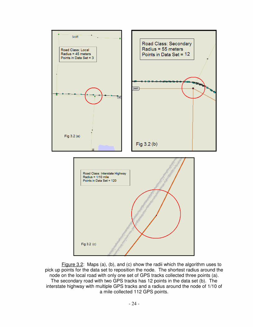
shortest link. Figure 3.2 shows the points picked up by the algorithm for each class
of road.
- 24 -
Figure 3.2: Maps (a), (b), and (c) show the radii which the algorithm uses to pick up points for the data set to reposition the node. The shortest radius around the
node on the local road with only one set of GPS tracks collected three points (a). The secondary road with two GPS tracks has 12 points in the data set (b). The
interstate highway with multiple GPS tracks and a radius around the node of 1/10 of a mile collected 112 GPS points.

- 25 -
The most accurate location of the node is the closest perpendicular distance
to the center of the GPS tracks. The center of the GPS tracks however cannot be
found by simply averaging the longitude and latitude of the GPS tracks around the
node. Only if there is an equal amount of data on both links and in both directions,
will the average location of the GPS tracks be the correct location for the new node.
In order to prevent the data from being skewed based on unevenly distributed data,
the spatial average of GPS tracks is taken in both directions. First the data is
divided into two sets, matched by link ID. Then for each link the algorithm uses the
in-degree and out-degree heading of the link into or out of the node. If the root node
is an A node the out-degree heading of the link gives the heading for which the link
exists the node. For a root B node, the value of the in-degree is used. This is the
link heading and will be used to separate the data around the node by direction.
Points in the data set which have a heading within plus or minus 20-degrees of the
link heading are collected into one data set. Points within plus or minus 20-degrees
of the 180-degree opposite of the link heading are collected into another set. Any
remaining points are discarded. It is possible to initially collect data from other links
so the process of separating the data ensures the data is valid.
Links with data from only one direction of travel will have only one data set
per link. Estimating where the other direction of travel might be and locating the
node at the midpoint between the estimated and the real data is beyond the scope of
this thesis. Therefore, this algorithm will place the node using only the data in one
direction of travel. As data becomes available the nodes can be aligned again.

- 26 -
3.4 Repositioning the Node
The final step is to find the geographical average of the different data sets.
There should be at least two data sets for each node, and four if there is data for two
directions of travel. The data sets are divided by direction and by link ID. There
must be a minimum of one point associated with each link in order for the algorithm
to work. Figure 3.3 demonstrates the process of collecting multiple spatial averages
to find the new longitude and latitude of the node. In the figure there are more
northbound GPS tracks than southbound. If the data were not split the spatial
average of these points would be skewed to the right. Since the points are divided
by direction and link, the results are less sensitive to uneven data availability.

- 27 -
Figure 3.3: Interstate – 35 outside of Dallas, TX The red square bounds the points which were picked up by the algorithm. The values, (X1, Y1) and (X2, Y2), are the spatial averages of the data for southbound traffic on Link A and Link B respectively. The values, (X3, Y3) and (X4, Y4), are the spatial averages for northbound traffic on Link A and Link B. The green square is the value of (X, Y), the new longitude and latitude of the node.

- 28 -
3.5 Implementation of the Simple Route Algorithm
The alignment of a simple route containing only nodes with two emanating
links containing data succeeds in moving the nodes to a longitude and latitude that
are closer to the GPS tracks. An advantage of this algorithm is that is uses the
position of real GPS data to determine the best location for the node representing
the road in the digital map. However, this algorithm is sensitive to data sets which
are distributed irregularly in space. Three test cases of the simple route algorithm
are evaluated in this section.
Figure 3.4: Route Alignment Test 1: 5100 Irving Blvd, Dallas, TX
The algorithm moves 3 out of the 4 nodes to a location exactly between
eastbound and westbound traffic. The node farthest to the left is not moved far
enough north, but rather is placed directly aligned with the westbound traffic. The

- 29 -
value of the latitude which the algorithm assigns to the node is either accurate or
significantly closer to position of the GPS tracks. The values of longitude, however,
changed more than desired. Each point is aligned closer to the data in some cases
the algorithm shifted the node to the right or to the left. This occurred because of
uneven data sets. Since GPS tracks are only collected every three seconds the
GPS tracks are not perfectly distributed along the links. Also curvature in the road
can cause the spatial average of the GPS tracks to deviate from the proper location
of the node. The last node needs to be manually moved to its proper location. The
algorithm does not move the last node in the route.
Figure 3.5: Route Alignment Test 2: Royal Lane, Meaders, TX

- 30 -
The second test area in Meaders, TX moved every node to the GPS tracks.
This setting is a series of grid like intersections with data only on one main road.
Again the last link in the set needs to be manually edited and moved to its proper
location. The concern with moving these nodes is that the original angle of the
intersection is preserved or kept as close to the original as possible. Three of the
nodes are successfully moved to the GPS tracks without significantly changing the
angle of the intersection. The data is fairly evenly distributed so there was not much
lateral deviation in the movement. However one of the nodes was shifted
significantly due to a change in density of the data. The algorithm moves the nodes
to GPS tracks; however it does not always preserve the original angle of the
intersection.
Figure 3.6: Route Alignment Test 3: N. Mill St, Lewisville, TX

- 31 -
This specific route closely aligned with the GPS data. N. Mill St only has two
sets of GPS tracks going in opposite directions. The algorithm places all the nodes,
except the last one in the route, closely to the GPS tracks. There are some angle
variations from the original map. This is partly due to sparse data, but also because
the original road map seems to be misplaced. The data on College Rd, intersecting
N Mill St., suggests that the entire road should be shifted up. The user of the
algorithm must be careful to notice situations where intersections are moved
significantly. It could be that the algorithm misplaced the node, but also it could
mean that multiple roads in the digital map need to be edited.
3.6 Performance of the Algorithm
The algorithm worked well to place the node into a midpoint between the
different directions of traffic along the path of the GPS tracks. The problem however
is that the data becomes skewed by irregular data. The algorithm seems to perform
better with smaller data sets. Figure 3.4 has the most data and Figure 3.6 has the
leas data. While the placement of the nodes is consistent with the GPS tracks no
matter what the size of the GPS data sets, a lateral shift along the path of the data
occurs when the data sets are larger. Also the placement of nodes along curved
roads does not work well with an algorithm using a formula for spatial averages to
relocate the nodes.

- 32 -
Chapter 4: Node Alignment at Branched Intersections ___________________________________________________________________
Correct positioning of the intersections in a digital map is important for the
overall accuracy of the map but is also in improving the efficiency of the navigation
system. A node which defines the spatial location of an intersection has three or
more emanating arcs. These nodes provide an anchor for the adjacent road
segments. Since intersections spatial locations are so important, a more precise
method is presented in this chapter to align the intersection with the surrounding
GPS tracks.
4.1 Theory
For the purpose of this algorithm an intersection is defined as any node
having more than two links emanating from it. When a route is selected to be edited,
each node is assigned a link value. The link value is equal to the number of
emanating links from the node. If the link value is equal to two, then the algorithm
will execute the method presented in the previous chapter, where the node is moved
as if it is a shapepoint. If the node has more than two emanating the algorithm will
execute a separate function which will consider the position of every link surrounding
the node. In order to accurately place the intersection the angle of every incoming

- 33 -
link into the node needs to be considered. The theory behind this part of the
algorithm is to find a set of linear equations representing the incoming links for each
node to find its correct location in space, (Xo, Yo). Each link with data on it will have
an equation in the form of Y = mX + b. The algorithm will attempt to place the
intersection in the most accurate location based on the data that is available.
For each link the algorithm will create a set of points which are neither too
close nor too far from the node in question. From these points a median heading on
a degree scale from 0 to 180. In other words all data points in the set will not be
distinguished by direction. That is if the heading of the track is greater than 180
degrees subtract 180 from it. GPS tracks with 180 degree opposite values of
heading will have the same median heading. The tangent line is the point of interest,
not which direction along the tangent the GPS track follows. The tangent of this
value will be the slope of the linear segment to be considered. The next step is to
find a value of the y-intercept, b. The data set for every link is divided by direction
and a least squares linear regression is run on the data points to produce a value of
the y-intercept. After regressing each data set, a series of linear equations will be
evaluated to find values of (Xo, Yo). The center of mass of these values will be the
location where the node is moved to. A more detailed explanation of the process is
discussed below.
4.2 Data Collection: Estimating the proper area from which to collect data
An important consideration is what of the available data to use in the
algorithm. How much and which of the data should be used will be determined in
the first step of the intersection alignment process. Some subset of the GPS tracks
will be used but too much data could adversely affect the results. The data set of
each link needs to include points that are close to the node in question but not too

- 34 -
close. The data needs to be chosen so that an accurate median heading of the link
into the root node can be found. When visually examining the intersection, it is clear
to the eye where the correct position of the center of the intersection is. An
algorithm is needed to use the same principles in a computational manner. GPS
tracks at the center of the intersection are bunched together and there are tracks
with headings different than the headings of the links. This is called the muddled
effect. The following intersection is an example of an intersection which the
algorithm will move.
Figure 4.1: Sample Intersection: “Muddled Effect”
The intersection node in Figure 4.1 needs to be moved down and to the right in order
to be properly aligned with the center of the intersection. The GPS tracks in the

- 35 -
middle of the intersection cross paths perpendicularly. Tracks from turning vehicles
lie just outside of where the intersection should be located. The combination of
crossing GPS tracks and turning vehicle tracks creates a muddled effect around the
center of the intersection. This data is difficult to decipher in this area. This
“muddled” area is where vehicles are either turning or are crossing paths. It is
important to exclude the muddled area from the data collected on the link. In order
to find the area on the link to which collect GPS points with a consistent heading,
data from primary roads, secondary roads, and divided roads which have
intersections are studied to find the size of the muddled area. The following is a plot
of the headings of GPS tracks collected along a link. The x-values [-20, 20]
represent the distance from the intersection node. Negative x-values are GPS tracks
to the left of the intersection and positive x-values are GPS track to right of the
intersection.
- 36 -
0
20
40
60
80
100
120
140
160
180
-20 -15 -10 -5 0 5 10 15 20
Distance along link (m)
Hea
ding
(deg
rees
)
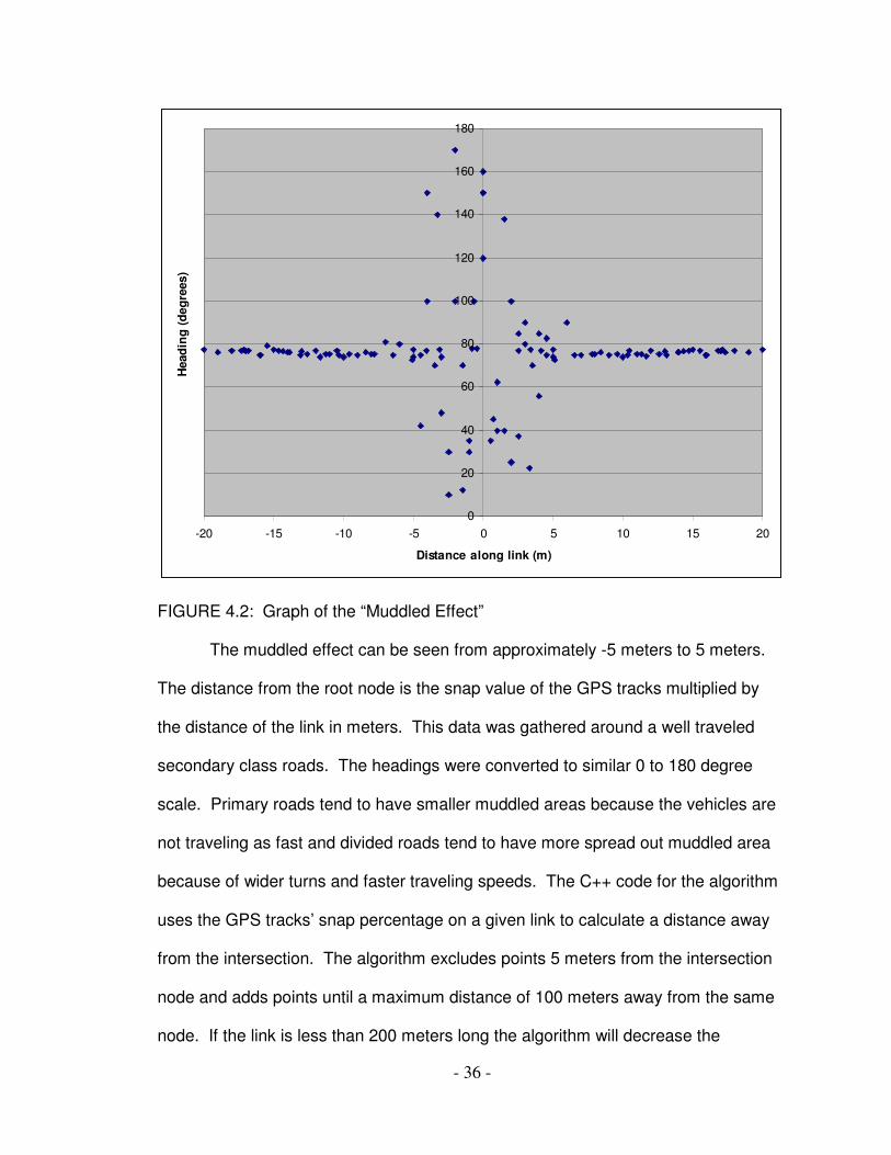
FIGURE 4.2: Graph of the “Muddled Effect”
The muddled effect can be seen from approximately -5 meters to 5 meters.
The distance from the root node is the snap value of the GPS tracks multiplied by
the distance of the link in meters. This data was gathered around a well traveled
secondary class roads. The headings were converted to similar 0 to 180 degree
scale. Primary roads tend to have smaller muddled areas because the vehicles are
not traveling as fast and divided roads tend to have more spread out muddled area
because of wider turns and faster traveling speeds. The C++ code for the algorithm
uses the GPS tracks’ snap percentage on a given link to calculate a distance away
from the intersection. The algorithm excludes points 5 meters from the intersection
node and adds points until a maximum distance of 100 meters away from the same
node. If the link is less than 200 meters long the algorithm will decrease the

- 37 -
maximum distance to less than half of the length of the link. Therefore, in order for
this method to work the link must be longer than 10 meters and have GPS points
between the 5 meters and the maximum distance. Figure 4.3 shows the points
which the algorithm picked up for each link.
Figure 4.3: GGD Data Collection 8500 Greenville Ave Points that were picked up by the algorithm are boxed at each link. Most links collected points from 5 meters to 100 meters from the node. However the link north of the intersection is shorter than 200 meters, so points were collected from 5 meters to half of the length of the link. 4.3 Finding a Median Heading, the “Slope” of Y= mX +b Equation
After gathering the most points on each link emanating from the arc the
median heading of the points associated with each link is found. The median
heading is chosen as opposed to the average heading because it is less sensitive to
outliers. The median is the middle value of a sorted vector. The algorithm gathers

- 38 -
the headings from all the points in the collected data set then sorts the points by
heading. A pointer to the middle of the vector references the median heading of the
data. If there is outlying data or if the road changes direction in the first 100 meters
from the intersection, the median heading is the most reliable result for the heading
of the link into the node. The heading is needed to find the slope of linear equation
for the link entering the node. Since the algorithm will use the tangent of the
heading, headings can be converted to a 0 to 180 degree scale. Lines with 180-
degree opposite headings have effectively the same slope.
FIGURE 4.4 Headings
For example, a line directed toward 225-degrees has the same slope as a line
directed toward 45-degrees. Since tangent (225) = tangent (45), the 225-degree
heading is transformed to 45-degrees by subtracting 180. The heading is then
converted to a slope value, “m”, by converting degrees to radians and then taking
the tangent of the angle in terms of radians. After this process is run on every link
emanating from the node there is an array which stores all of the m-values for each
link in the set.

- 39 -
4.4 Creating Separate Data Sets: ggdA and ggdB
The GPS data sets from each link contain tracks from vehicles traveling on
both sides of the road. There is a separation of the tracks between the two lanes.
Figure 4.5 depicts the separation of traffic on the same road traveling in different
directions. Depending on the type of road the lanes the separation of lanes varies.
The algorithm will create an equation for both directions of travel. The original data
set of points collected on each link is copied before changing the headings. The
data set needs to be separated again into ggdA and ggdB. GGD is a data structure
which CoPilot uses to store GPS tracks. These GGD sets are broken down by link
and by direction of travel. The set ggdA contains tracks from the same link which
have heading approximately 180 degrees less than the other points.
- 40 -
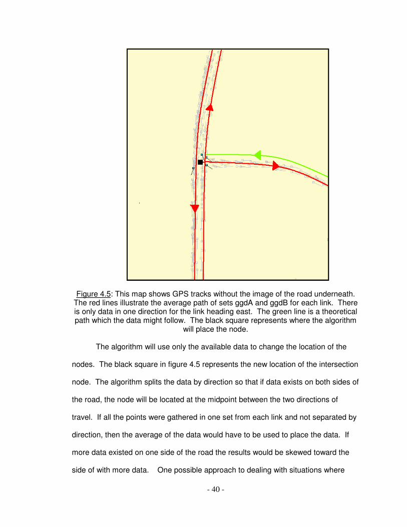
Figure 4.5: This map shows GPS tracks without the image of the road underneath.
The red lines illustrate the average path of sets ggdA and ggdB for each link. There is only data in one direction for the link heading east. The green line is a theoretical path which the data might follow. The black square represents where the algorithm
will place the node. The algorithm will use only the available data to change the location of the
nodes. The black square in figure 4.5 represents the new location of the intersection
node. The algorithm splits the data by direction so that if data exists on both sides of
the road, the node will be located at the midpoint between the two directions of
travel. If all the points were gathered in one set from each link and not separated by
direction, then the average of the data would have to be used to place the data. If
more data existed on one side of the road the results would be skewed toward the
side of with more data. One possible approach to dealing with situations where

- 41 -
data only exists on one side of the road is to estimate where the other side of the
road is located and place the node at a midpoint between the two. In theory this
method is the most accurate; however, this algorithm uses only available data to
place the nodes and links. The focus of this thesis is to adjust the links and nodes of
a digital map using real GPS data; aligning the map using real and estimated data is
an area of further exploration.
4.5 Regression of GGD data sets to find a Y-intercept Once a value for the slope has been found for each link and the data points
have been separated, the next step is to run a linear regression on each set of points
to find a value for the y-intercept. For each set of data points, the algorithm creates
a linear equation in the form of Y = mX + b. The method of finding the slope, m, is
discussed in the previous section. Now the algorithm will find a value for b, the y-
intercept. A least square regression is run to find this value. The least squares
method is a procedure for using sample data to find the estimated regression
equation. The sample data are the ggdA and ggdB sets for each link. The values of
(x, y) are the longitude and latitude of the each of the GPS tracks. The least squares
method minimizes the sum of the squares of the deviations between the latitude of
the GPS tracks, y, and an estimated value for y. The least square formula is as
follows:
Min ( )� − 2ˆ ii yy
where: yi = value of the latitude for the i th GPS track in the set iy = estimated value of the latitude for the i th GPS track in the set

- 42 -
FIGURE 4.6: This graph shows the distribution of each expected value of y. The actually values are plotted as squares. The same distributions exist also for the x-values. The regression minimizes the sum of the squares of the deviations to develop a line of best fit. The least squares regression is used to find a value of b, the y-intercept.
The least squares regression is ideal because good results can be obtained
with relatively small data sets. Roads with relatively little data will have small data
sets after points are collected from 5m to 100m on the link and separated by
direction. The derivation of the formulas for least squares regression is based on
minimizing the sum of the squares of the deviation. The equations below describe
the computations the algorithm uses to produce a value for the y-intercept.
Let y = b1x + bo where b0 is the value of the y-intercept to be found
- 43 -
( )( )
( )�
�−
−−=
21xx
yyxxb
i
ii
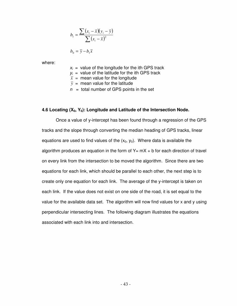
xbyb 10 −= where: xi = value of the longitude for the ith GPS track yi = value of the latitude for the ith GPS track x = mean value for the longitude y = mean value for the latitude n = total number of GPS points in the set 4.6 Locating (X0, Y0): Longitude and Latitude of the Intersection Node.
Once a value of y-intercept has been found through a regression of the GPS
tracks and the slope through converting the median heading of GPS tracks, linear
equations are used to find values of the (x0, y0). Where data is available the
algorithm produces an equation in the form of Y= mX + b for each direction of travel
on every link from the intersection to be moved the algorithm. Since there are two
equations for each link, which should be parallel to each other, the next step is to
create only one equation for each link. The average of the y-intercept is taken on
each link. If the value does not exist on one side of the road, it is set equal to the
value for the available data set. The algorithm will now find values for x and y using
perpendicular intersecting lines. The following diagram illustrates the equations
associated with each link into and intersection.

- 44 -
Solving for the x and y coordinate is done by the following process:
Figure 4.7: Equations Y= m1X+b1 and Y= m2X+b2 are solved to find a value for (X0,Y0). Equations 3 and 4 are also solved to find a value for (X0,Y0).
Subtracting Eq. 2 from 1,
y = m1 * x + b1 -- [ y = m2 * x + b2 ] 0 = (m1 - m2)* x + (b1 – b2)
Solving for x, (b2 – b1) = (m1 - m2)* x x = (b2 – b1) (m1 - m2)
Solving for y, y = m1 * x + b1
y = m1 * (b2 – b1) + b1 (m1 - m2)

- 45 -
For every pair of perpendicular links, the algorithm computes a value for
(X0,Y0). For an intersection with three links emanating from the node there will be
two values of (X0,Y0). For a 4 – way intersection will have four values of (X0,Y0) as
each set of perpendicular lines is solved. There will be a set of (X0, Y0) values for
each intersection. The center of mass of this set will be the new location of the
intersection, (X,Y). The node will be re-assigned this longitude and latitude. In
North American the value for longitude is negative and latitude is positive. The final
step of this algorithm is to verify that the movement of the node is correct. The new
position of the node needs to be within a given radius of the original position of the
node.
The example shown in Figure 4.3 is revisited to show proper alignment of the
intersection to the center of the GPS tracks. The following figure shows the new
location of the node to represent the center of the intersection more accurately. The
red square is the location of the node before alignment.
Figure 4.8 (a)

- 46 -
Figure 4.8 (b): Table of Values for Values of (X,Y) for the New Location of the Node Longitude Latitude
(X0,Y0) -96753613 32893676
(X1, Y1) -96753376 32893541
(X2, Y2) -96753372 32893576
(X3, Y3) -96753587 32893619
(X, Y) -96753403 32893618
The table in Fig 4.8 (b) shows the values of (X,Y) which the algorithm found by
solving a set of linear equations. Figure 4.8 (a) labels which links are used by the
algorithm to produce each value of the new longitude and latitude of the node. The
final value of (X,Y) is the center of mass of (X0,Y0), (X1, Y1), (X2, Y2), (X3, Y3). The
algorithm successfully relocates the intersection to a better location based on the
GPS data.

- 47 -
Chapter 5: Shapepoints In the previous chapters only the spatial alignment of nodes is considered;
however, often the link deviates from the GPS tracks even when the end nodes are
correctly positioned. There are many contributing factors. Moving the nodes to their
proper location can cause deviation from the GPS tracks between the nodes. Most
likely the link is not aligned properly to begin with. The algorithm does not
distinguish whether the link was originally misaligned or whether the movement of
nodes caused the misalignment. The link is straightened before the process of
adding shapepoints begins. Shapepoints divide the link into smaller adjoining linear
segments. The basic problem of this part of the algorithm is how to adjust a series
of linear segments in order to best align with the GPS tracks. The goal is not to
perfectly match the linear segments with each GPS track but rather to create an
approximate linear-type curve in the link. This chapter will lay out a theory of two
processes which are used to better align digital map road segments to the GPS
tracks associated with the links.
FIGURE 5.1: US RT 71/ 59 through Pullman, AR The series of maps show the progression of adding shapepoints to links to mimic the curvature in the road. Figure (a) shows the road as is in the digital map; Figure (b) shows the map after GPS tracks have been loaded; Figure (c) shows the road once the shapepoints have been added; and finally (c) shows the alignment of the GPS tracks and the road.

- 48 -

- 49 -
5.1 Determining Where Shapepoints Are Needed
The degree of curvature in roadways is represented in digital maps using
linear segments. Nodes act as anchors to the linear link segments. Shapepoints
create smaller piecewise linear segments which mimic the curvature of the road as
represented in the GPS tracks. As shown in Figure 5.1 when GPS tracks are
superimposed onto the map, it is easy to see where shapepoints are needed to bring
the link closer to the data. The challenge lies in how to program an algorithm to find
the best location for these shapepoints. Too many shapepoints are undesirable
because they take up memory in the database of the road network. The desired
amount of shapepoints is the minimum amount necessary to create the effect of
curvature using linear segments to follow the GPS tracks. Another concern is how
many shapepoints to add. The number of shapepoints added to each link could be a
fixed number; however, linear road segments will need none, and some road
segments with sharper curves will need many. The first step in the shapepoint
algorithm is to straighten the link and remove any existing shapepoints. Leaving
existing shapepoints in place assumes that the original data is correct. The premise
of this thesis is that the original digital road map network has error and is in need of
improvement. It is best to assume that the original shapepoints of the route being
edited does not have the correct number and location of shapepoints. Therefore, the
algorithm will first straighten the link before determining the number and location of
shapepoints that need to be added. Two approaches to adding shapepoints will be
discussed in this chapter. Both begin by straightening the link. One method is a
binary stepwise function which divides the link in half and checks if or where a
shapepoint is needed. The function continues to divide link segments in half until
each breakpoint is at a minimum distance from the nearest GPS points associated

- 50 -
with the link. The other method which is explored is a search for the greatest
deviation of the GPS points from the link. Shapepoints are then added in the correct
location until the distance of the greatest deviation is reduced to a minimum
acceptable distance. Figure 5.2 is a visualization of how shapepoints will be moved
to bring the link closer to the GPS tracks.
FIGURE 5.1: The thick line represents the path of the GPS tracks and then thin straight line represents the straightened link. New shapepoints (blue circles) are added to the link and positioned to align with the GPS tracks path. 5.2 Binary Approach to Adding Shapepoints
The snap values of the GPS tracks will remain unchanged. The GPS tracks
will not be re-snapped after the link is straightened. Even though the original route is
selected because it needs to be better spatially aligned, it is assumed that the
original curvature of the link in the digital map is closer to the actual road compared

- 51 -
to the straightened link which the algorithm uses to add shapepoints. Therefore the
snap percentage values which associate each GPS track with a position between
the A and B node on the link will not change.
The algorithm first locates the midpoint of the link. All GPS points with the
same link ID are collected. Each set of data points per link is sorted by snap
percent. The midpoint of the link is associated with a snap value of 50%. A GPS
data set is created containing all GPS points with a snap percent from 45% to 55%.
If the data set is empty then the percentage parameters are increased to 40% to
50%. If the data set is still empty the algorithm moves on to the next link. After a
sufficient set of data points is collected, the average latitude and longitude of the
data is found. If the distance between the average spatial position of the data set
and the midpoint of the link is greater than 5% of the link length, a shapepoint is
added to the link. The new shapepoint has the longitude and latitude of the average
position of the data set.
Once the midpoint has been found the algorithm moves to the midpoint of the
first half and then to the midpoint of the next half. The same process of gathering a
data set from the link data is done for snap values from 20% to 30% and from 70%
to 80%. If these sets are empty the parameters are not expanded and the algorithm
moves on the next node. Shape points are added in the 1st half of the link and the
2nd half of the link if the distance from the point on the link to the average spatial
position of the data set is greater than 5% of the link length. If the minimum distance
is met, meaning the GPS tracks are less than 5% of the link length, then the
algorithm moves on to the next link. If needed shapepoints are needed then the
algorithm moves to a position of 12.5%, 37.5%, 67.5%, and 77.5% on the link and
repeats the same process adding shapepoints where necessary.

- 52 -
FIGURE 5.2: A Breakdown of how the algorithm steps through the link position to check for GPS data associated with link. The position of snap values on a link is show in (a). The progression of checkpoints is showing in (b). (a)
(b)
The algorithm continues to break down the link into sections until the
minimum distance is satisfied. The advantage of this approach is that once a
section of the link is positioned correctly using shapepoints, the algorithm exits
without having to take any extraneous steps. Also the algorithm continues until the

- 53 -
link is sufficiently aligned to the path of the GPS tracks. The distance of 5% of the
link length is a parameter which can easily be changed to make the process of
adding shapepoints more precise.
5.3 Greatest Deviation Approach to Shapepoint Addition
As in the previous method of adding shapepoints, after the nodes have been
moved to a new location the links straightened removing any shapepoints. Even
after the link is straightened the same GPS data is still associated with the link. The
next step will be to reintroduce shapepoints if necessary to add curvature to the
linear links. Without any shapepoints the link is the shortest distance between the
locations of its nodes. Shapepoints divide the link into smaller adjoining linear
segments. Adding shapepoints will increase the total length of the link in order to
simulate any curve which is shown in the GPS tracks.
The algorithm will find where the GPS tracks deviate the greatest distance
from the link. Assuming the A and B nodes are correctly positioned the point of
greatest deviance in the middle section of the link. The algorithm will find where the
greatest perpendicular distance between the links and the GPS tracks is located. If
this value is greater than a given threshold value a shapepoint is be added to the
link. The shapepoint now needs to be assigned a location in space. It will move the
center of the link to the spatial average of the GPS tracks which are farthest away
from the link. This process should be run on every link in the selected route until
each link roughly follows the track of the corresponding GPS data. Figure 5.4
demonstrates this process.

- 54 -
FIGURE 5.4: Diagram of Greatest Deviation Approach to Adding Shapepoints Each iteration of the algorithm adds a shapepoint until the link is satisfactorily
aligned to the GPS tracks associated with the link.
In order to figure out where to place the shapepoints, the GPS data needs to
be averaged. Geometrically the location should be at the greatest perpendicular
distance from the link. In order to find that point the GPS points need to be
averaged into packets if data. The parameter which determines the size of the
packet will depend on the type of road being considered. Each packet will represent
a spatial average of the GPS data in that set. The GPS packet with the greatest
distance from the link will be the location of the new shapepoint. However, direction
needs to also be considered. Each of the GPS tracks has a direction of travel on the
road. Only GPS tracks with the same direction of travel should be averaged together
in a grouping. In order to place the shapepoint in the most accurate location, it

- 55 -
needs to be placed in what would be the centerline of a two-way road. If the road is
a one-way in direction, this step is not a consideration. If data is available in both
directions, the shapepoints needs to be placed in the spatial average of two GPS
packets in the opposite direction of travel. If only one direction of data exists, the
shapepoint needs to be placed a set distance to left of the GPS packet. This
distance is a parameter that will depend on the type of road selected for spatial
alignment.

- 56 -
Chapter 6: Conclusion The aim of this thesis is to align sections of digital road maps to real GPS
data. An algorithm which moves a set of n links and n+1 nodes is presented in
detail. One algorithm handles simple routes with data only available for one link
entering a node and one link exiting a node. The algorithm is designed based on the
characteristics of the data set. The algorithm uses only the heading and spatial
position of the GPS tracks in the data set to determine the best location for the
selected route. GPS tracks from vehicles on the road are currently the most reliable
source of data available for improving the spatial attributes of the digital
representation of the road network. The algorithm only works on a small set of links
selected by the user. The algorithm is designed this way to limit the effect of bad
data on the realignment of the map. Theoretically an algorithm which acts
automatically as new data becomes available on the road network would be the
most efficient solution for the task of improving the accuracy of digital maps.
However, GPS technology is not yet reliable enough and the digital road network is
not close enough to positional accuracy that an independent algorithm could be
trusted to fix the digital road map. Human and machine interaction is a necessary
condition for creating accurate digital maps at this point in time. This thesis is a first
step toward the process of improving the accuracy of digital maps. Perhaps

- 57 -
sometime soon GPS technology will be reliable enough and digital maps close
enough to create an algorithm to automatically improve the spatial characteristics of
digital maps.
6.1 Implications
Increasing the positional accuracy of digital maps improves the overall quality
of navigation systems. The map matching process is one of the major components
of navigation software. If the GPS position of the vehicle actually corresponded to
the exact position on the digital map, the map matching process would be quick and
simple. The efficiency and accuracy of GPS navigation systems greatly benefit from
having accurate maps.
Satellite aerial photography has an important application for digital maps.
Google Maps11 developed a hybrid map that is a combination of an aerial
photograph with the lines of the road network on the map. Accurate digital maps are
important in order to underlay the satellite photograph. The slightest deviation from
the road’s true position and it becomes obvious where the line of the road is not on
top of the picture of the road. As the accuracy of digital maps improve it will be
easier to use photography as a backdrop for digital maps. The user will be able to
see not only the location and names of the streets, but also landmarks and other
physical structures which will help in the navigation process.
6.1: Strengths and Weaknesses
The best feature of the algorithm presented in this thesis is that it uses real
GPS data to realign the digital road map. However, one of the major drawbacks to
this method is that GPS data can be flawed. Outlying data skews the results of the
route alignment algorithm significantly. While the data can be removed it is 11 <maps.google.com>
- 58 -
nonetheless an important concern. Also the size of the data sets used to align the
route affects results of the algorithm. In many cases the nodes were not placed in
the correct location because the data set was either too large or too small. When
the link curves around the node the data set needs to be smaller and when the links
are straight coming into and out of the node, the data sets need to be larger. The
intersection algorithm uses a minimum distance of 5m and a maximum of 100m, but
these number can be changed based on the type of link and the amount of data
available for collection.
An advantage of the algorithm which moves the intersection is that it does not
rely on the position of the GPS tracks but rather uses the heading of the tracks. This
reduces the sensitivity of outlying data. The positions of the GPS tracks are used to
find a value for the Y-intercept of the linear equation for each link. The downside to
this approach of doing a regression analysis to find a set of linear equations for each
node is that the results are not as reliable when the data sets are small. The data
must be accurate and follow a linear path if the data sets are small in order to
correctly relocate the intersection node.
6.2: Future Research
The algorithm developed in this thesis is developed using C++ code in the
CoPilot program. The method of this algorithm can be adapted to other programs by
changing the code to fit the specific needs of the program. The algorithm uses
universal coding principles which can be translated into other programming
languages as well.
The parameters associated with data collection are important for results of
the algorithm. Interstate highways have more data and generally longer links than
primary and secondary roads. The algorithm would improve by adjusting the area of

- 59 -
collection for GPS tracks on the link based on the amount of data available. Also,
curvature on the road affects the effectiveness of the algorithm. The results would
be more accurate if the size of the data sets is changed based on the path of the
GPS tracks.
This thesis is part of a first step towards improving the accuracy of digital
maps. The algorithm is sensitive to the effects of bad data. Because of this effect,
the algorithm is implemented on a small scale basis so that the user can inspect the
data and the surrounding network before changing the spatial attributes of the roads.
If a separate algorithm could identify bad GPS by examining the characteristics of
the tracks and their relation to any other GPS tracks associated with the link, it would
save a significant step of the process. Removing bad data from the entire data set is
also feasible and would allow the maps with GPS data overlaid to be cleaner and
easier to follow.

- 60 -
WORKS CITED AND REFERENCED Clark, Rex L. “Topographic mapping with GPS”, Engineering & Technology for Sustainable World, vol. 4, no. 5, May, 1997. El-Rabbany, Ahmed. Introduction to GPS: the Global Positioning System, Artech House, Boston, 2002. Federal Aviation Administration Satellite Navigation Product Teams, <http://gps.faa.gov> GCSD Press Release, “Harris Corporation Awarded $200 Million Contract for U.S. Census Bureau’s MAP/TIGER Accuracy Improvement Project,” June 25, 2002. Hoffmann-Wellenhoff, B., H. Lichtenegger, and J. Collins. GPS: Theory and Practice, Springer-Verlag, New York, 1993. Okuno, A. and M. Shikada, “Real-time renewal of the digital map for local government by using remote sensing and GPS” Proceedings of SPIE, pp. 271-279, 2004. Marx, R.W. The TIGER System: Yesterday, Today, and Tomorrow, Cartography and Geographic Information Systems, 17(1): 89-97, January 1990. Rogers, S., Langley, P., & Wilson, C. “Learning to predict lane occupancy using GPS and digital maps.” Proceedings of the Fifth International Conference on Knowledge Discovery and Data Mining. San Diego, CA: ACM Press, 1999. Schroedl, Stefan, Kiri Wagstaff, Seth Rogers, Pat Langley, and Christopher Wilson. “Mining GPS traces for map refinement”, Data Mining and Knowledge Discovery, pp. 59-87, 2004. Shibata, M. “Updating of Digital Road Map”, Proceedings of the Vehicle Navigation and Information Systems Conference, pp. 547-550, 1994. TIGER/Line Metadata, <http://www.census.gov/geo/www/tlmetadata/metadata.html> U.S. Dept. of Commerce, Bureau of the Census. GEOGRAPHIC BASE FILE/DUAL INDEPENDENT MAP ENCODING (GBF/DIME), 1980 [Computer file]. Washington, DC: U.S. Dept. of Commerce, Bureau of the Census [producer], 1980. Ann Arbor, MI: Inter-university Consortium for Political and Social Research [distributor], 1985.

- 61 -
U.S. Dept. of Commerce, Bureau of the Census "The Census Bureau's GBF/DIME System: A Tool for Urban Management and Planning." Washington, DC: 1980. “The Story of DIME: A Progress Report,” The GIS History Project, The University of Buffalo, 1997. “Cartography and Geographic Information Systems”, Government Information Quarterly, Vol 17. NO 1, 1990.

- 62 -
Appendix A:
Code for Simple Route Alignment void CEditorDrawer::MoveLinkRouteToGPS(unsigned long mapID, ListMgr<GP_LinkData> &tmpLinkList) { if (2 > tmpLinkList.Count()) return; GGData* ggdSet = NULL; unsigned long ggdCount = 0; ggdSet = Map_GetGGDataSet(mapID, ggdCount ,1); if( 0 == ggdCount) return; // get points only in current view, ggdPoints GGData* ggdPts = new GGData[ggdCount]; unsigned long ggdPoints = 0; TGLongPoint tPoint; for(unsigned long i = 0; i < ggdCount; i++) { tPoint.x = ggdSet[i].m_Lon; tPoint.y = ggdSet[i].m_Lat; if (m_BoundingRect.Contains(tPoint)) { ggdPts[ggdPoints] = ggdSet[i]; ggdPoints++; } // Resnap Values GPSMgr_ReSnapGGDPoints(mapID, ggdPts, ggdPoints); LinkAngleTable glLinkAngle; LinkAngle* laVals = new LinkAngle[tmpLinkList.Count()]; GridID laGID = 0; for (unsigned long i = 0; i < tmpLinkList.Count(); i++) { if(laGID != tmpLinkList[i]->Grid) ::Grid_GetNet()->GetGridTable(tmpLinkList[i]->Grid, glLinkAngle); laVals[i].InDegrees(glLinkAngle[tmpLinkList[i]->Link].InDegrees()); laVals[i].OutDegrees(glLinkAngle[tmpLinkList[i]->Link].OutDegrees()); } for (unsigned long i = 0; i < tmpLinkList.Count(); i++) MoveLinkToGPS(mapID, *tmpLinkList[i], ggdPts, ggdPoints, laVals[i]); delete [] laVals; delete [] ggdPts; }

- 63 -
bool CEditorDrawer::MoveNode_TwoLinks(NodeCoords &tmpNode, GGData* ggdSet, unsigned long ggdCount, GP_LinkData link, LinkAngle la) { LinkBaseTable glLinkBase; NodeCoordTable glNodeCoords; LinkShapeTable glLinkShape; ShapePointTable glShapePoints; int linkAngle; ::Grid_GetNet()->GetGridTable(link.Grid, glLinkBase); ::Grid_GetNet()->GetGridTable(link.Grid, glNodeCoords); ::Grid_GetNet()->GetGridTable(link.Grid, glLinkShape); TGLongPoint pt,ptA,ptB; TGLongRect bound; // include the a node in the bounding rectangle ptA.x = glNodeCoords[glLinkBase[link.Link].ANode()].Longitude(); ptA.y = glNodeCoords[glLinkBase[link.Link].ANode()].Latitude(); // if this is the first link start with the A node being the original bounding rect bound.SetBounds(ptA.x,ptA.y,ptA.x,ptA.y); if (glLinkShape[link.Link].ShapeCount()) { ::Grid_GetNet()->GetGridTable(link.Grid, glShapePoints); // include any shape points for(unsigned short j = 0; j < glLinkShape[link.Link].ShapeCount(); j++) { if (link.Link != glLinkShape[link.Link].LinkNum()) break; // add offsets to last point pt.x += glShapePoints[glLinkShape[link.Link].ShapeIndex()].XOffset(); pt.y += glShapePoints[glLinkShape[link.Link].ShapeIndex()].YOffset(); bound.Include(pt); } } // include the B node in the bounding rect ptB.x = glNodeCoords[glLinkBase[link.Link].BNode()].Longitude(); ptB.y = glNodeCoords[glLinkBase[link.Link].BNode()].Latitude(); bound.Include(ptB); // add a buffer for the bounds

- 64 -
//bound.Expand(abs((bound.ptA.x - bound.ptB.x))/2,abs((bound.ptA.y - bound.ptB.y))/2); int linkDist; linkDist = sqrt((double)((ptA.x-ptB.x)*(ptA.x-ptB.x) + (ptA.y-ptB.y)*(ptA.y-ptB.y))); bound.Expand(linkDist/2, linkDist/2); GGData* ggdPts = new GGData[ggdCount]; unsigned long points = 0; for (unsigned long i = 0; i < ggdCount; i++) { // pt.x = ggdSet[i].m_Lon; // pt.y = ggdSet[i].m_Lat; // if the ggd point is in the rect add it to the use list // if (bound.Contains(pt)) { ggdPts[points] = ggdSet[i]; points++; } } if ( 0 == points ) return false; // snap subset of points // GPSMgr_ReSnapGGDPoints(mapID, ggdPts, points); unsigned long node; // get end point if(link.bIsAtoB) { node = glLinkBase[link.Link].BNode(); pt.x = glNodeCoords[node].Longitude(); pt.y = glNodeCoords[node].Latitude(); linkAngle = la.OutDegrees()*2; } else { node = glLinkBase[link.Link].ANode(); pt.x = glNodeCoords[node].Longitude(); pt.y = glNodeCoords[node].Latitude(); linkAngle = la.InDegrees()*2; } linkAngle = (linkAngle + 90)%360; int linkAngleA; int linkAngleB; if(180 > linkAngle) { linkAngleA = linkAngle; linkAngleB = linkAngle + 180; } else

- 65 -
{ linkAngleB = linkAngle; linkAngleA = linkAngle - 180; } long radius = 0; switch(link.Class) { case 1: case 2: if (1400 < linkDist) { radius = 1400; } else { radius = (3*linkDist)/4; } break; case 3: if (900 < linkDist) { radius = 900; } else { radius = (3*linkDist)/4; } break; case 4: if (500 < linkDist) { radius = 700; } else { radius = (3*linkDist)/4; } break; case 6: if (400 < linkDist) { radius = 400; } else { radius = (3*linkDist)/4; } break; case 7: radius = 600; break; case 8:

- 66 -
if (300 < linkDist) { radius = 300; } else { radius = (3*linkDist)/4; } default: break; } GGData* ggdADirection = new GGData[points]; GGData* ggdBDirection = new GGData[points]; int nodePTSA = 0; int nodePTSB = 0; for (unsigned long i = 0; i < points; i++) { long dist = sqrt((double)((pt.x - ggdPts[i].m_Lon)*(pt.x - ggdPts[i].m_Lon) + (pt.y - ggdPts[i].m_Lat)*(pt.y - ggdPts[i].m_Lat))); int nodeHeading = ggdPts[i].m_HeadingX10 / 10; if (dist < radius) { if(linkAngleA-20 < nodeHeading && linkAngleA+20 > nodeHeading) { ggdADirection[nodePTSA] = ggdPts[i]; nodePTSA++; } else if (linkAngleB-20 < nodeHeading && linkAngleB+20 > nodeHeading) { ggdBDirection[nodePTSB] = ggdPts[i]; nodePTSB++; } } } long latdistA = 0; long londistA = 0; long latdistB = 0; long londistB = 0; for (unsigned long i = 0; i < nodePTSA; i++) { if ( 0 == i ) { latdistA = ggdADirection[i].m_Lat; londistA = ggdADirection[i].m_Lon; } else { latdistA = (latdistA + ggdADirection[i].m_Lat)/2; londistA = (londistA + ggdADirection[i].m_Lon)/2;

- 67 -
} } for (unsigned long i = 0; i < nodePTSB; i++) { if ( 0 == i ) { latdistB = ggdBDirection[i].m_Lat; londistB = ggdBDirection[i].m_Lon; } else { latdistB = (latdistB + ggdBDirection[i].m_Lat)/2; londistB = (londistB + ggdBDirection[i].m_Lon)/2; } } delete [] ggdPts; delete [] ggdADirection; delete [] ggdBDirection; if ( 0 == nodePTSA && 0 == nodePTSB ) return false; else if (0 == nodePTSA) { tmpNode.Longitude(londistB); tmpNode.Latitude(latdistB); } else if (0 == nodePTSB) { tmpNode.Longitude(londistA); tmpNode.Latitude(latdistA); } else { tmpNode.Longitude((londistA + londistB)/2); tmpNode.Latitude((latdistA + latdistB)/2); } return true; }

- 68 -
Appendix B:
Code for Intersection Alignment
#define MAXDIST_GGD 63 // 100 meters converted to measurements for link #define MINDIST_GGD 3 // 5 meters converted bool CEditorDrawer::MoveNode_Intersection(unsigned long mapID, GridID grid, NodeCoords &tmpNode, GGData* ggdSet, unsigned long ggdCount, unsigned long node, LinkBaseTable &glLinkBase, LinkID* linkList, unsigned short sLinkCnt) { // get only the points around the intersection node GGData* ggdPts = new GGData[ggdCount]; unsigned long ggdPtsCnt = 0; for (unsigned long i = 0; i < ggdCount; i++) { //ptTest.x = ggdSet[i].m_Lon; //ptTest.y = ggdSet[i].m_Lat; //long dist = sqrt((double)((ptOrig.x - ptTest.x)*(ptOrig.x - ptTest.x) + (ptOrig.y - ptTest.y)*(ptOrig.y - ptTest.y))); LinkID link = ggdSet[i].m_SnapLink; for (unsigned long j = 0; j < sLinkCnt; j++) { if(link == linkList[j]) { ggdPts[ggdPtsCnt] = ggdSet[i]; ggdPtsCnt++; } } } double *mValA = new double[sLinkCnt]; double *mValB = new double [sLinkCnt]; double *bValA = new double [sLinkCnt]; double *bValB = new double [sLinkCnt]; double *bVal = new double [sLinkCnt]; double *linkHeading = new double[sLinkCnt]; double X=0; double Y=0; // go through each link to find slope to intersection and y intercept for(unsigned long lks = 0; lks < sLinkCnt; lks++) { LinkID linkID = linkList[lks]; unsigned long ulMaxDist = MAXDIST_GGD; //link must be twice max distance

- 69 -
if((2 * MAXDIST_GGD) > glLinkBase[linkID].Distance()) ulMaxDist = glLinkBase[linkID].Distance() / 2; bool bToA = false; if(glLinkBase[linkID].ANode() == node) bToA = true; //make a list of GGD points within intersections range on this link GGData* linkGGD = new GGData[ggdPtsCnt]; unsigned long linkGGDCnt = 0; for(unsigned long pts = 0; pts < ggdPtsCnt; pts++) { if(ggdPts[pts].m_SnapLink == linkID) { double percent = (double)ggdPts[pts].m_SnapPctX100/100.00; if(!bToA) // reverse percentage if we are look at the b node percent = 100.0 - percent;
double min = 100.0 * (double) MINDIST_GGD / glLinkBase[linkID].Distance();
double max = 100.0 * (double) ulMaxDist / glLinkBase[linkID].Distance();
if(percent > min && percent < max) { linkGGD[linkGGDCnt] = ggdPts[pts]; linkGGDCnt++; } } } GGData* oldGGD = new GGData[linkGGDCnt]; GGData* ggdA = new GGData[linkGGDCnt]; GGData* ggdB = new GGData[linkGGDCnt]; int countA = 0; int countB = 0; double heading; // make backup list of ggd points and change original list to only have values between 0-180 degrees for(unsigned long i = 0; i < linkGGDCnt; i++) { oldGGD[i] = linkGGD[i]; heading = linkGGD[i].m_HeadingX10; if(heading < 1800) { heading = heading; } else { heading = heading - 1800; }
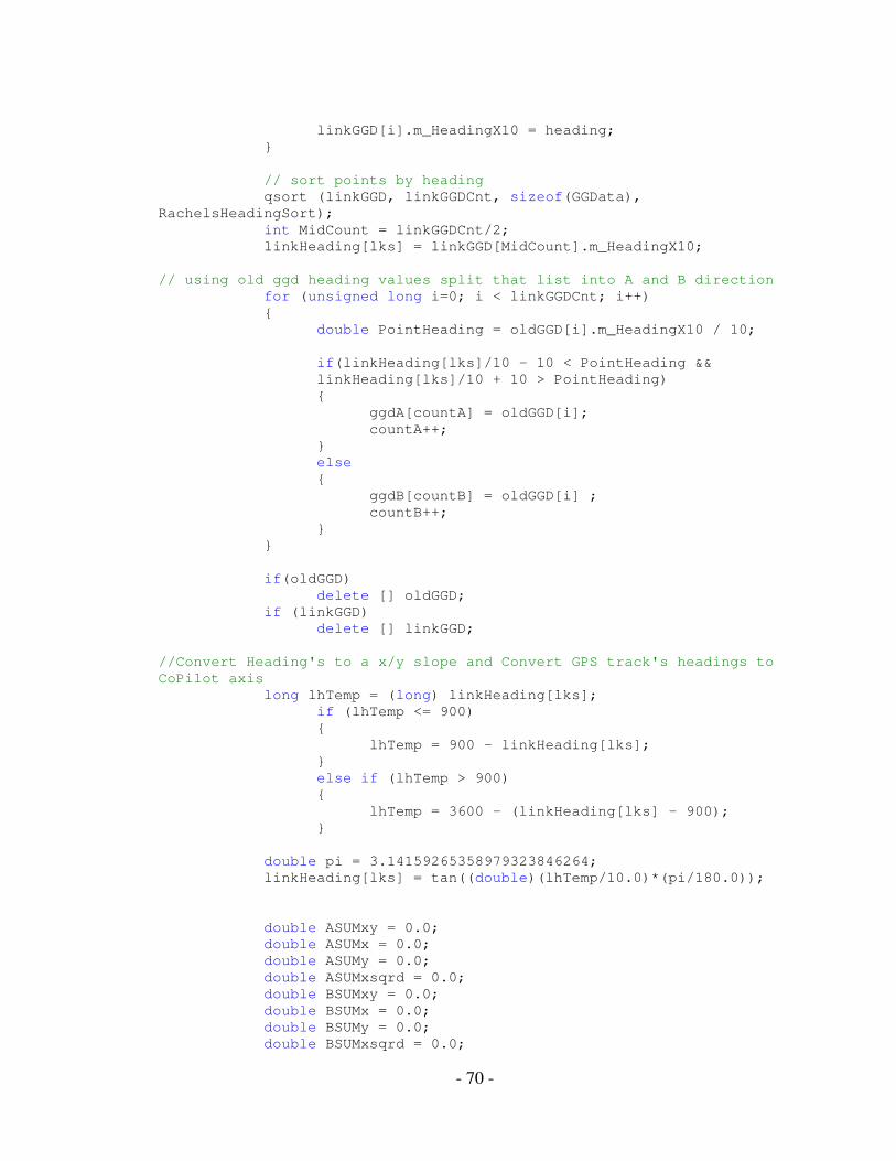
- 70 -
linkGGD[i].m_HeadingX10 = heading; } // sort points by heading qsort (linkGGD, linkGGDCnt, sizeof(GGData), RachelsHeadingSort); int MidCount = linkGGDCnt/2; linkHeading[lks] = linkGGD[MidCount].m_HeadingX10; // using old ggd heading values split that list into A and B direction for (unsigned long i=0; i < linkGGDCnt; i++) { double PointHeading = oldGGD[i].m_HeadingX10 / 10;
if(linkHeading[lks]/10 - 10 < PointHeading && linkHeading[lks]/10 + 10 > PointHeading)
{ ggdA[countA] = oldGGD[i]; countA++; } else { ggdB[countB] = oldGGD[i] ; countB++; } } if(oldGGD) delete [] oldGGD; if (linkGGD) delete [] linkGGD; //Convert Heading's to a x/y slope and Convert GPS track's headings to CoPilot axis long lhTemp = (long) linkHeading[lks]; if (lhTemp <= 900) { lhTemp = 900 - linkHeading[lks]; } else if (lhTemp > 900) { lhTemp = 3600 - (linkHeading[lks] - 900); } double pi = 3.14159265358979323846264; linkHeading[lks] = tan((double)(lhTemp/10.0)*(pi/180.0)); double ASUMxy = 0.0; double ASUMx = 0.0; double ASUMy = 0.0; double ASUMxsqrd = 0.0; double BSUMxy = 0.0; double BSUMx = 0.0; double BSUMy = 0.0; double BSUMxsqrd = 0.0;

- 71 -
// go through a direction ggdpoints for the link and find values for y intecept for (unsigned long j=0; j<countA; j++) { ASUMxy = ASUMxy + (ggdA[j].m_Lon/1000000.0) * (ggdA[j].m_Lat/1000000.0); ASUMx = ASUMx + (ggdA[j].m_Lon/1000000.0); ASUMy = ASUMy + (ggdA[j].m_Lat/1000000.0); ASUMxsqrd = ASUMxsqrd + (ggdA[j].m_Lon/1000000.0)*(ggdA[j].m_Lon/1000000.0); } // go through B direction ggdpoints for the link and find values for y intecept for (unsigned long j=0; j<countB; j++) { BSUMxy = BSUMxy + (ggdB[j].m_Lon/1000000.0) * (ggdB[j].m_Lat/1000000.0); BSUMx = BSUMx + (ggdB[j].m_Lon/1000000.0); BSUMy = BSUMy + (ggdB[j].m_Lat/1000000.0); BSUMxsqrd = BSUMxsqrd + (ggdB[j].m_Lon/1000000.0)*(ggdB[j].m_Lon/1000000.0); } if(0 < countA) { mValA[lks] = (double)(countA*ASUMxy - ASUMx*ASUMy)/(countA*ASUMxsqrd-ASUMx*ASUMx); bValA[lks]= (double) (ASUMy*1000000.0/countA) - (mValA[lks]*ASUMx*1000000.0/countA); } if(0 < countB) { mValB[lks] = (double)(countB*BSUMxy - BSUMx*BSUMy)/(countB*BSUMxsqrd-BSUMx*BSUMx); bValB[lks]= (double) (BSUMy*1000000.0/countB) - (mValB[lks]*BSUMx*1000000.0/countB); } if(0 == countA && 0 == countB) { mValA[lks] = 0.0; bValA[lks] = 0.0; mValB[lks] = 0.0; bValB[lks] = 0.0; } else if(0 == countA) { mValA[lks] = mValB[lks]; bValA[lks] = bValB[lks]; } else if(0 == countB) { mValB[lks] = mValA[lks]; bValB[lks] = bValA[lks];

- 72 -
} bVal[lks]= (bValA[lks] + bValB[lks])/2; if(ggdA) delete [] ggdA; if(ggdB) delete [] ggdB; } //FIND Value Of (X,Y) Location of intersection double *Xo = new double [sLinkCnt]; double *Yo = new double [sLinkCnt]; // (Xo,Yo) the location of the intersection of two Perp. Links // (X,Y) is the center of mass of every (Xo, Yo) for(unsigned long lks = 0; lks < sLinkCnt; lks++) { if (lks+1 <= sLinkCnt) { Xo[lks] = (bVal[lks+1]-bVal[lks])/(linkHeading[lks]-linkHeading[lks+1]); Yo[lks] = linkHeading[lks]*Xo[lks] + bVal[lks]; } else { Xo[lks] = (bVal[0]-bVal[sLinkCnt])/(linkHeading[sLinkCnt]-linkHeading[0]); Yo[lks] = linkHeading[sLinkCnt]*Xo[lks] + bVal[lks]; } X = (X + Xo[lks])/2; Y = (Y + Yo[lks])/2; } if(ggdPts) delete [] ggdPts; delete [] mValA; delete [] mValB; delete [] bValA; delete [] bValB; delete [] linkHeading; return true; }

- 73 -
Appendix A:
Structure of the Algorithm
LinkBaseTable glLinkBase; NodeCoordTable glNodeCoords; LinkShapeTable glLinkShape; ShapePointTable glShapePoints; ::Grid_GetNet()->GetGridTable(link.Grid, glLinkBase); ::Grid_GetNet()->GetGridTable(link.Grid, glNodeCoords); unsigned long node; LinkID linkList[15]; if(link.bIsAtoB) node = glLinkBase[link.Link].BNode(); else node = glLinkBase[link.Link].ANode(); short sLinkCnt = 0; //Count the number of links to determine which function to use for(unsigned short i = 0; i < glLinkBase.Count(); i++) { if (node == glLinkBase[i].ANode()) { if(HasGGDPoints(i, ggdSet, ggdCount)) { linkList[sLinkCnt] = i; sLinkCnt++; } } else if (node == glLinkBase[i].BNode()) { if(HasGGDPoints(i, ggdSet, ggdCount)) { linkList[sLinkCnt] = i; sLinkCnt++; } } } bool ret = false; NodeCoords tmpNode; tmpNode.Latitude(glNodeCoords[node].Latitude()); tmpNode.Longitude(glNodeCoords[node].Longitude()); tmpNode.IsJunction(glNodeCoords[node].IsJunction()); if(2 < sLinkCnt) {
ret = MoveNode_Intersection(mapID, link.Grid, tmpNode, ggdSet, ggdCount, node, glLinkBase, linkList, sLinkCnt);
}

- 74 -
//else only two links attached to the node if(2 == sLinkCnt) ret = MoveNode_TwoLinks(tmpNode, ggdSet, ggdCount, link, la); if(false == ret) return;
ret = g_editGlobals.GetEditOvrdValidator()->ModNode(link.Grid, node, tmpNode);
Map_Refresh(mapID); } int RachelsHeadingSort (const void * a, const void * b) { const GGData * as = (const GGData *)a; const GGData * bs = (const GGData *)b; if (as->m_HeadingX10 < bs->m_HeadingX10) return -1; else if (as->m_HeadingX10 > bs->m_HeadingX10) return 1; else
return 0; }