00

0 -4Co 0

_-- Technical Doc~ument 721(N

A RADAR SEA CLUTTER MODEL FORIn. ATMOSPHERIC DUCTING CONDITIONS

I F. Perry SnyderMarine Sciences and Technology Department

August 1984

Prepared forNaval Air Systems Command

ca...

S5~Eiý 0q '{984

Approved for public release, distribution unlimited. " "F--

N CD

NAVAL OCEAN SYSTEMS CENTERSan Diego, California 92152

84' 0 0 6 9;

NAVAL OCEAN SYSTEMS CENTER SAN DIEGO, CA 92152

AN ACTIVITY OF THE NAVAL MATERIAL COMMAND

J.M. PATTON, CAPT, USN R.M. HILLYERCommander Techmical Director

ADMINISTRATIVE INFORMATZON

The work discussed here was performed under prog'Cam element 61153N(NOSC 532-MP07) for the Naval Air Systems Command. The work wasperformed between October 1979 and December 1983. This document was

approved for publication 5 April 1984.

Released by Under authority of

J. A. Ferguson J. H. Richter, Head

Modeling Branch Ocean and AtmosphericSciinces Division

RHB

UNCLASSIFIED

K REPORT DOCUMENTATION PAGEI1a Rfl E0X W1C Y ~aN5ATlw lbI RE5TRICTIMAMUGS

UNCLASSIFIED* 2. SECflSTY CLASSIFICATION4 AUTHORITY 3 DIsTRIUUTON/VAA84aETY OF R(EPORT

*2b DEcLASSIFCA1NDOW'ik*RADIO SCHEDWL Approved f'or pL... th release; distribution unlimited.

4 PERFORMMIG ORiGANIZATION REPORT #4UMSER(SI 5 MONITORING ORGAMZATION REPORT NUMUERISI

NOSC TD 721

4 NAM~E OF PEROaRMIN ORGANIZATION 6b OFIC SYMBOL 7&~si NAM OF MONTORING OmoGs1tzATIO.

* Naval Ocean Systcms Center JCode S446C ADRESS (Coy State 8..dZIPCocl) ?b ADDRESS (Cay. Str.ato SZIP Co*AP

*San Diego, CA 92152

I ($a NAME OF FUNDING /SPOMSRW.;ORGANIZATION Sb OFFICE SYMBOL 9 PROCUREMENT INSTRIUMENT IDENTIFICATION NUMBER

Naval Air Systems Command jI '3c ADDRESS (CaY Stare itAZP Ca&e, 10 SOURCE OF FUND"N NUMBERS

PROGRAM ELEMENT NO PROJECUT NO TASK NO WR0WTN

QWashington, DC 20361 61153N WRO2101 532-MP07 wM0P7 LwT"

11 TITLE i~a*c~.Seewaw CIsdtUýoVt

A RADAR SEA CLUTTER MODEL FOR ATMOSPHERIC DUCTING CONDITIONS

12 PEFISOMALAUTHORISI

F. P. Snyder

134 TYPE OF REPORT 13b TIME COVERED 14 DATE OF REPORT IV*.,. VmitF 0ev) 15 PAME COUNT

Final FROM Oct 79 10 Dec 83 31 July 1984 3916 SUMPEMENTAXY NOTATION

17 COSATI CODES 10 SUIJECI TIAbIS ICarvat?, on, ,o.Wra IF~mw PWM d ~*mvsrA by bled ntWv*.WI

FIELD GROUP sue GRU Atmospheric ductingIntegrated Refractive Effects Prediction System (IREPS)Sea clutter

19 ABSTRACT (CO~an ro.*, *,fi5 neeeawv antdomoyr by Maca ,..nioarl

An updated surface clutter computer model for IRLPS is presented, along with some details of the computer implementation. Ananalysis also is presented which Lýdicates the sensitivity of the ulidel to variations in the environmental parameters required aS input to thecomputer program. 9linally. a quantitative validation effort is discussed, though in terms only of data acquired for a single location and asingle frequency due .0 flimited assets.

21ONIRIBTIONAVAAWTVOf ASTRAT 2 ABSTRACT SECURITY CLASSIFICATION

Z2 M FI~"OEItrXL220 TEL! P'lOht.E(,rbA,*eA.e C**ie 22C OFFICE SYMBSOL

1%P ndr(619) 225-7400 Code 544

DD FORM 1473. 84 JAN A" OTHIOýfol"I'oNs ARE OBSOLETE SLE

CONTENTS

INTRODUCTION ........................

THE PROPAGATION AND CLUTTER CROSS SECTION MODE.S ..... 3

EFFECTS OF REFRACTIVITY LAYER BOUNDARY PERTY2RBATUIBS . . . . 15

MODEL VALIDATION . . . . . . . . . . . . . . . . . . . . . . 21

CONCLUSIONS AND RECOMMENDATIONS ............... 26

REFERENCES ....................... .. 39

Accession ForNTIS GRA&I • @ .

DTIC TABUnonnounced 5Justificatio1

By

Distribution/-

Availability CodesAvail and/or'-

"Dist Special

I+++,1

f INTRODUCTION

The Integrated Refractive Effects Prediction System (IREPS) should

consider sea clutter effects under atmospheric ducting conditions. The IREPS,

undergoing research and development at Naval Ocean Systems Center (NOSC), is

intended to provide a shipboard environmental data processing and display cap-

ability to assess refractive effects of the lower atmosphere for naval EM

systems. Although intended to be incorporated eventually as a part of the

Tactical Environment Support System (TESS), the IREPS is currently configured

as an interim version based on a Hewlett-Packard 9845 desktop calculator. A

comprehensive discussion of the IREPS capabilities is presented by Hitney etL

al. (1981), while a discussion of the IREPS propagation models is presented by

Hattan (1982). -

Numerous limitations of the IREPS models are listed by Hitney et al.

(1931), among which is the fact that surface clutter (land or sea) is not

included in the calculation of radar detection ranges. A clutter computer

model was developed and was first described by Snyder (1979). Some

modifications have subsequently been made to this model and the updated model

has been implemented in - computer program in FORTRAN (the language of the

original IREPS). This updated model, along with some details of the computer

implementation, is discussed in this document. Also presented is an analysis

indicating the sensitivity of the model to variations in the environmentaJ

parameters required as input to the computer program.

Snyder (1979) concluded that the sea clutter model developed appeored to

be adequate, at least qualitatively, for an elevated layer, ground based duct

environment, but that some sort of quantitative "validation" effort should be

conducted before implementation into IREPS for shipboard use. Because of

1

manpower and money limitations, an extensive validation effort could not be

undertaken. However, using essentially "free" facilities on a "not-to-inter-

fere" basis, validation data were acquired for a single location and a single

frequency. That validation effort is also discussed in this document.

2

THE PROPAGATIOP AND CLUTTER CROSS SECTION MODELS

Snyder (1979) and Hitney et al. (1981) both point out the occurrence of

two types of atmospheric ducts which can be expected to greatly influence sea

clutter. One is the evaporation duct, which is formed by the sea surface and

the near surface minimum in the refractive index prolile, which is in turn

determined mainly by the vertical distribution of water vapor resulting from

evaporation. 'The other is a surface based duct formed by an elevated refrac-

tive layer.

The propagation environments resulting from the two types of ducts are

uniquely different and can be expected to result in two different effects on

sea clutter. The evaporation duct would tend to enhance clutter signals over

extended areas, whereas the ground based duct formed by an elevated layer

would result in clutter signal enhancement only from discrete ranges.

Propagation in the two different environments would also best be considered

using two different formulations. Vertical dimensions for the evaporation

duct are on the order of metres to very f ew tens of metres and a waveguide

mode formulation would be appropriate for this type of duct. Vertical

dimeneions for the ground based duct formed by an elevated refractive layer

are typically on the order of many tens of metres to a few hundred metres and

ray-optical formulations would be appropriate here.

The clutter model developed for the IREPS is based on a ray-optical

propagation formulation and is therefore most applicable to the surface based

duct formed by an elevated refractive layer. The geometrical basis for the

propagation formulation is developed in the following way. The propagation

environment is assLmed to be two dimensional, with the earth represented by a

cylinder and propagation in a plane transverse to the cylinder axis. Thus,

earth curvature is considered in the direction of propagation but is ignored

3

transverse to the propagation direction. A classical conformal transtormation

to Maxwell's equations in cylindrical form is employed, converting the geome-

try from cylindrical to rectangular (Cartesian). This transformation has been

discussed in the context of earth flattening by Richter (1966) and has been

widely applied in radiowave and radar propagation problems when earth curva-

ture in the direction of propagation is an important factor. The net effect

of the transformation is to change from the cylindrical geometry with refrac-

tive index given by n to the rectangular geometry with refractive index given

by n multiplied by exp(z/a), where a is the radius of the earth hnd, to first

order in 1/a, and z is essentially the altitude above the eartu (see Figure

1).

Th ray path trajectories are determined from the classical eikonal

expression (Jones, 1979)

(n =~Vn (1)

ds ds

where

s = %rc length along a ray path

n = n(r) = index of refraction at rA A A

S= position vector (x rx + y r + z r )A A

x, y, z = unit rectors

Let

dr.t = - (i = x, y, z) (2)i ds

and use the fact that (Vn)i = :n/ ri to rewrite (1) in rectangular form as

4

d (ntx bn dx t (3a)dB x ~x dS -x

d (nt (3b)ds ?s y

dbn dzT (nt- d = t (3c)ds z ds z

Rewrite (3a) as

dn. dtx bn (4)tx ds ds -x

With dn/ds in component form

da _ ndx + n dz +n t.

dTs Tx ds by ds + z ds ar. i.

equation (4) becomes

dtx bn rL5n I 53 tx r ti (5) -

which can be generalized to all three coordinate directions. Assuming homo-bn bngeneity in both horizontal directions (T T o)the components of (5)

bx ~y,-3come

dtx txtz dn (6a)

C n dz

5

dt _a± 2ds- nd (1-t2) (6c)

If t = 0 initially, corresponding to a ray having no initial transverse

component, then (6b) shows that ty 0 always. Making this assumption and

transforming to the angular variable given by t = cosO and t = sinO (0 isx z

the ray angle with respect to the horizontal) leads to the expressions

d= n ldn cos; dz sinO (7)d-s n d-z ' d~s " '

The refractive index in (7) is given in terms of the original (cylindri-

cal) refractive index as

n = n(z) exp(z/a) (8)

Because the atmospheric refractive index n(z) is only slightly greater than

unity, it is convenient to write n(z) = 1 + 8n(z) where 6n << 1.

-4Typically, 6nsIo- so in order to have a number of more convenient magnitude,

6the "refractivity" N has been defined to be N = (n - 1) x 106 = 6n x 10

Expaniding the exponential term in (8) and using the modified refractiv-

ity, defined as M N + 10 z!a, the refractive index can be written as

n = 1 + I- 6 M (9)

Substituting (9) into (7), assuming paraxial. rayti ane writing the angle in

milliradiant (i = 1030) yields the differential forus

d dZ : 13dM 'dx '10)d dz1

6

Integrating the first expression in (10) yields

2 2 (11)Po + 2 (N M)0 0

where P is the angle at the modified refractivity M resulting from initial

angle p at M Integrating the second, expression in (10) with the assump-OO 0.

tion that dM/dz is constant yields

P " Po'JC -(12)

10 ( ). .

where the initial condition x = 0, P = P is ass'-,med. The result in (11) is L

simply a stateme-* . Snell's law in the paraxial approximation and is inde-

pendent of the iay the modified refractivity varies with height. The result 2in (12), ncw.ever, is valid only 41f the modified refractivity varies linearly

with height. The modified refractivity profile for the clutter model is thus

asaumed to be linearly segmented with height.

Some properties of ray paths which are important to the question of sea

clutter under ducting conditions are shown in Figure 2. A surface based duct

resulting from an elevated refractive layer is shown diagramatically in Figure

2 as a trilinear M-profile. Assume that a ray source is located at some

height, such as position A in the Figure. From (11) a ray will be concave

apward within the first linear segment of the profile and concave downward

within the second. Further, the magnitude of the slope of any ray trajectory

wil.l be the same at all. points within the profile with the same M-value,

provided of course, that the ray reacl 5 s the particular point at al.l. For

example, a ray launched horizontally (labelled (A] in rigure 2) at A will be

7

continualiy turned upward until reaching the first change in profile slope and "1

will then begin turning downward. As the ray approaches the height A', where

the M-value is the same as at A, the ray ta '-e.tory will again approach hori-

zontal and continue turning downward, th1is being "reflected" at height A'.

The ray trajectory again changes concavity where the M-profile slope changes

and is again horizontal at height A, being reflqcted upward at this height.

The ray is thus "ducted" or "trapped" between A and A'.

Consider a ray launched downward at A with such an angle that the contin-

ual upward turning will result in a horizontal trajectory just above the

surface. Such a ray, labeled [B] in 1,igure 2, will be trapped between the

heights of B and B', as shown in Figure 2. Any 7ay launched below this ray

will reach the lower surface (which is necessary before the ray can contribute

to sea clutter) and be reflected according to the usual. laws of reflection at

a plane interface. Thare is a launch angle for which a ray will just become

horizontal as it approached C' in Figure 2. Such a ray, labeled [C] in Figure

2, will be reflected downward at C' and will thus be trapped between the

surface and C'. Any ray launched below this ray (such as ray [D] in Figure 2)

will reach the heiiht C' at a non-zero angle and continue upward, escaping

through the top of the duct. There is thut? a range of downward launch angles

for which rays will be both trapped in the duct and reflected off the lower

(sea) surface. By symmetry and reciprocity arguments, there is also a family

of rays with upward launch angles which will be trapped in the duct as well as

be reflected off the lower surface. It is these two families of rays which

contribute to sea clutter enhancement under conditions when an elevated re-

fractive layer produces a surface based duct.

In the ray-optical propagation model, a single ray is envisioned as

departing the radar, propagating forward, then to be refracted by the atmo-

8

- - - - - ° I

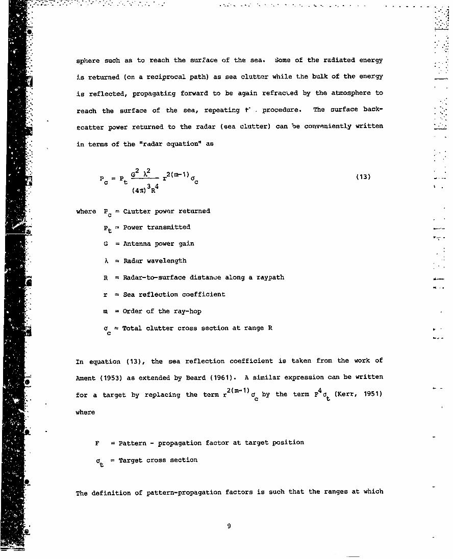
"sphere such as to reach the surZace of the sea. Some of the radiated energy

is returned (on a reciprocal path) as sea clutter while the bulk of the energy

is reflected, propagating forward to be again refract.ed by the atmosphere to

reach the surface of the sea, repeating t . procedure. The ourface back-

scatter power returned to the radar (sea clutter) can be conveniently written

in terms of the "radar equation" as

2 2"":GG 2 2(m-1) (13)PC Pt - r ac(3Sc = t 3 c

(4,n) 34R14

where Pc = Ciutter power returned

Pt = Power transmitted

G = Antenna power gain

K = Radar wavelength

R = Radar-to-surface distanue along a raypath

r = Sea reflection coefficient

m = Order of the ray-hop

a = Total clutter cross section at range RC

In equation (13), the sea reflection coefficient is taken from the work of

Ament (1953) as extended by Beard (1961). A similar expression can be written

2(m-1) 4for a target by replacing the term r a by the term F a (Kerr, 1951)

c t

where

F w Pattern - propagation factor at target position

a = Target cross section

The definition of pattern-propagation factors is such that the ranges at which

a 9

target detection can occur (without clutter) are given by

R < FORfs (14)

where Rf s is the range to target detection in free space. If clutter is

present, a working definition of target detection is the simultaneous satis-

faction of (14) and the requirement that the target power returned exceed the

clutter power returned.

SR< FeRf s AND PT > Pc (15)

Swhere PT 3s the returned target power. In terms of the various cross

sections, (15) is equivalent to:

F < (a /a) 4r~m' (16)

This model is based on a ray-optical propagation model. To accomodate a non-

ray optics model, such as the equivalent single mode model used in the IREPS

for ductcd propagation (Hattan, 1982), note tht .16) can be used provided

only that a way to determine F as a function of r~ns is available.

The area extensive cross-section of sea return is a function of many

variables, including sea state, angle of incidence, aspect angle, radar

wavelength and polarization. The clutter cross section model adapted for use

with the ray path popagation model was de'veloped at Georgia Institute of

Technology and is commonly known as the GIT sea clutter model (Trebits et al.,

1978). The model is semi-empirical and calculates the sea clutter cross

section normalized per unit area as a product of three factors: sea

• 10Se

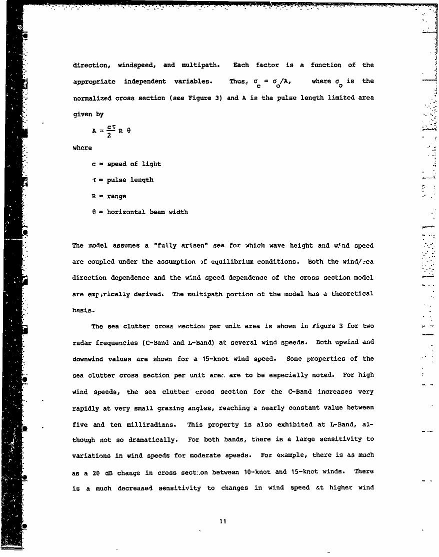
direction, windspeed, and multipath. Each factor is a function of the .4

appropriate independent variables. Thus, a = a /A, where o is thec 0 0

"normalized cross section (see Figure 3) and A is the pulse length limited area

given by

A-R R2

where

c speed of light

T = pulse length

R = range

0 = horizontal beam width

The model assumes a "fully arisen" sea for which wave height and w.nd speed

are coupled under the assumption if equilibrium conditions. Both the wind/Zea

direction dependence and the wi.nd speed dependence of the cross section model --

are emrLrically derived. The multipath portion of the model has a theoretical

basis.

The sea clutter cross siection, per unit area is shown in Figure 3 for two

radar frequencies (C-Band and L-Band) at several wind speeds. Both upwind and

downwind values are shown for a 15-knot wind speed. Some properties of the

sea clutter cross section per unit arec. are to be especially noted. For high

wind speeds, the sea clutter cross section for the C-Band increases very

rapidly at very small grazing angles, reaching a nearly constant value between

five and ten milliradians. This property is also exhibited at L-Band, al-

though not so dramatically. For both bands, there is a large sensitivity to

variations in wind speeds for moderate speeds. For example, there is as much

as a 20 dB change in cross sect:.on between 10-knot and 15-knot winds. There

is a much decreased sensitivity to changes in wind speed at higher wind

•0 11

"speeds, although the clutter cross sections are much larger for higher wind

"speeds. Note also that the directional dependence of clutter cross section is

insensitive to the actual windspeed and grazing angle, although there is some

* -sensitivity to the radar band, with the larger directional dependence at

higher frequencies.

The computer implementation of the model was effected in the following

way. Reference modified refractivities are computed corresponding to the

*.- levels in Figure 2 at C'(denoted by Mu), at D (denoted by Md) and at A

(denoted by Kt). The occurrence of a surface based duct is determined if Mu

< Md and the radar is in the duct if Mt > Mu. If these are satisfied, the

i- launch angle d for the surface grazing ray ([B] in Figure 2) and the launch

angle (P ) for the ray just grazing at C'(C] in Figure 2) are computed. The

rays that are trapped and also contribute to sea clutter are found within the

Slimits Pu- PdI both above and below the horizontal. This fan of rays is

divided into 30 equally spaced rays (P ), and for each ray the following are

computed:

= grazing angle at sea surface for j-ray.

Puj surface distance for the upward launched j-ray to be "reflected"

and return to the sea surface.

pdj surface distance for the downward launched J-ray to reich the sea

surface.

Ap = skip distance for the j-ray puj + Pdj

a cj sea clutter cross section for j-ray (normalized per unit area)

12

*. I*- - - r I .

r sea surface reflection coefficient for j-ray

The •s are computed using (11) and the p's are computed by iterative applica-

"tion of (12) for each ray.

The propagation path is divided into 100 range bins of 2 )km each. A

recursive procedure is then employed to determine the contribution to the

total clutter power due to each successive hop for both the upward launched

and downward launched ray sets. Values within any given range bin are deter-

-* mined by linear interpolation between two j-rays if a single ray does not

"iand" within the bin. The 100 elements of the range bin array are finally

Smodlified to Include a preset but arbitrary target cross section and appropri-

ate roots are taken to provide the right hand side of (16).

The operational implications of the combined ray path propagation model

and normalized clutter cross section model can be qualitatively inferred from

the considerations of the individual aspects already discussed. It can be

expected, for example, that at high wind speeds, even moderately strong

surface based ducts will result in enhanced clutter ,effects. The clutter ring

"splitting," mentioned previously (Snyder, 1979) in regards to the USS ENTER-

PRISE demonstrations of the IREPS, can be inferred from the existence of two

sets of influential rays (the initially upgoing and downgoing launched

sets). The existence of clutter rings in only a limited angular sector might

be inferred by the directional dependence of the clutter -ross section, but

horizontal inhomogeneity in the environment would seem a more likely cause. -

The clutter effects model was coded and implemented into a special FOR-

TRAN version of the IREPS. Typical results 2re presented in the "coverage

diagrams" of Figures 4-6. A hypothetical C-Band radar with 100-nmi free space

13

detection range against a reference target of two square metres cross section

is assumed located at 140 feet height. As a reference, the coverage diagram

for a nonducted (standard) atmosphere with a 10-knot wind is shown in

Figure 4. Recall t:hat the darkened area of the diagram represents the

- range/height conditions where the radar would detect the target.

A coverage diagram for the same wind conditions, but for a surface based

duct, is shown in Figure 5. The elevated refractive layer causing this duct

" is loc?.ted at about 300 metres and is 40 metres thick. The M-unit deficit

- between the surfa,-'e and the layer minimum is 40 H-units. Notice the enhanced

coverage for l.ow altitudes to longer ranges. For this case, any clutter

effects are just barely observed. A coverage diagram for the same

refractivity profile but for a 15-knot wind is shown in Figure 6. For this

case, t)' predicted effects of clutter are quite dramatic. Within the darken-

ed areas of the diagram, target detection would be expected. However, within

the areas no longer darkened compared to Figure 5, the target would be wnde-

tectable compared to clutter. The presence of clutter in this case would

appear on a PPI type display as bright rings, masking the target.

4-i1

EFFECTS OF REFRACTIVE LAYER BOUNDJARY PERTURBATIONS

An important property of the clutter model is the ability to predict

characteristics of clutter rings. A crucial factor in this ability is the

properties of the vertical modified refractivity profile. Variations in the

2". profile boundaries can be expected to produce variations .,n the clutter ring

characteristics. For this reason, effects of both bulk and localized

variations in profile boundaries have been examined.

Typical sensitivities of computed clutter ring locations to bulk

variations in boundary heights for elevated layers are shown in Figure 7. The

figure shows the location of the first and second clutter rings for a

trilinear profile as a function of layer thickness and parametric in layer

height. In this example, variation in layer thickness results from changes in

the slope of the modified refractivity within the elevated layer with no

change in the height of the bottom of the layer, the slope of the lowest

region of the profile (called AM/Ah in Figure 7), or the net H-deficit

(called N4 in Figure 7). The geometrical change in the profile is shown in

the figure insert. The change in clutter ring location per metre change in

layer thickness is approximately 0.2 nmi for the first ring and 0.3 nmi for

the second. These results depend only very slightly on the layer height or

thickness.

An alterriate variation in layer thickness, resulting from raising the

height of the layer while maintaining a fixed gradient both within and below

the layer as well as a fixed M-deficit was also considered. For this situa-

t4'on, the change in clutter ring location per metre change in layer height is

approximately 0.1 nmi for the first ring and 0.2 nmi for the second. Just as

for the previous case, theps results are insensitive to the specific layer

height or thickness.

15

-M -1 ; ;7 _

From these and ott.er similar results, it is concluded that bulk changes

in refractive layer height or thickness on the order of a few metres will only

slightly change the apparent clutter ring location on a typical PPI display.

Bulk changes of such an order might be expected over short periods, perhaps on 4--

the order of a few tens of minutes. Over periods of a few hours or longer,

bulk changes on the order of tens of metres in refractive layer height or

thickness may be expected. For such longer periods, changes of a few miles in

clutter ring location might be expected.

The actual occurrence of clutter rings is a more sensitive function of

refractive layer configuration than is the variation in location. Changes in

layer height or thickness are usually accompanied by changes in M-deficit.

This results in changes in the grazing angle and consequently in the clutter

return signal. Bulk changes in height or thickness of elevated refractive

layers are thus expected to lead to clutter rings which fade "in-and-out" on a

typical PPI display while remaining nearly fixed in location...

The effects of bulk changes in the boundaries of the refractive layer

formed by a surface evaporation layer have also been considered. The

_. evaporation layer was modelled simply with a single negative M gradiernt at the

surface, changing to a positive gradient at height h as shown in the insert0

to Figure 3. Although ray optical methods are generally inadequate for

complete quantitative analysis of propagation in the evaporative duct, the

method is believed adequate to describe qualitative and quantitative trends

resulting from modifications in evaporative duct parameters. Two types of

changes were considered, one with constant layer strength (height) and vari-

able M-deficit and the other with Uixed M-deficit and variable layer

strength. Typical results for variable M-deficit are shown in Figure 8. In

the figure, an evaporation layer with mLnimum M-value at ten metres and vari-

16l"

able H-deficit is superimposed on a modified refractivity profile with a

50-matre-thick refractive layer at a height of 300 metres. The original

profile (without evaporation layer) produces a ground based duct with a 30 M-

unit deficit. A diagramatic picture of the modified refractivity profile is

*, included in Figure 8.

Figure 8 shows that the location of clutter rings is very insensitive to

the change in M-deficit. In fact, for the range of H-deficits considered, the

change in clutter ring location is less than 0.1 nmi. However, the clutter

return cross section is seen to be a sensitive function of the M-deficit,

increasing in excess of 3 dB for the range in M-deficit shown. Thus, for this

type of bulk profile modification, clutter rings would exhibit exceptional

spatial stability with variable intensity.

The alternate variation in evaporation layer, characterized by a fixed

value to M-deficit and variable layer height (ho of Figure 8), showed a signi-

ficant sensitivity of computed ring location to layer height (or layer

strength). Because the M-deficit remained constant, and therefore also the

grazing angle, the clutter model predicts this type of profile modification

produces no change in the clutter return signal.

The variations in clutter ring characteristics due to modelled variations

of an evaporation layer thus differ both qualitatively and quantitatively from

the results for variations of an elevated layer. In particular, clutter ring

location is reasonably stable for bulk variations in elevated layers, but

highly variable for bulk variations in evaporation laye,', Furthermore, much

larger changes in ring intensity would be expected for evaporation layer

variations.

Localized variations in layer boundaries were modelled in terms of spa-

tially periodic fluctuations of layer boundaries. Two forms of perturbations

17

7|

were considered, one a sinusoidal variation in evaporation layer strength

"(height) and the other an exponentially damped sinusoidal variation in refrac-

tivity at the boundary of an elevated refractive layer. Numerical integration

of the three-dimensional ray equation was used. The eikonal equation in

rectangular component form (see equation 5) was employed with the assumption

that bn/by = 0 so that n had only a two-dimensional vari&tion (z-vertically;

x-in the horizontal propagation direction). Also, an arbitrary initial ray

direction and position were permitted. The coupled equations (5) were solved

with a fourth-order Runge-Kutta routine using a comparison with second-order

to control step size adjustment.

The use of the raytrace formulation of (5) requires an analytic expres-

sion for the refractive index. In order to approximate the trilinear profiles 6-A

used previously, the procedure of Boo.s. (1977) was adopted. The steps in

this procedure are depicted in Figure 9. A prototype modified refractivity

profile composed of linear segments with slopes A is assum 1. The transition

from one slope to another is modelled by the analytic axpression (A). By an

appropriate selection of the "scale height" (H), the slope rapidly approaches

"A 1 for z < z 2 and A2 for z > z2 . A generalization to a multislope profile is

given by expression (B). The final analytic form of the modifi.ed refractivity

is found by integrating expression (B) and is given by expression (C). A

sample of the use of the algorithm to generate profiles is shown in Figure

10. In the figure, the prototype profile is trilinear and the results for two

scale heights (H = 20 km and 5 km) are included. A scale height of 5 km was

used for the modified refractivity profiles. -

Numerous raytraces were computed using a variety of modified refractivity

profiles. Sample raytraces showing the effects of the sinusoidal pertu'-

bations are given in Figure 11. The effects of a periodic elevated layer are

77 7:7--.-

shown in Figure Ila. The unperturbed refractivity profLle is the same as in

Figure 10. The sinusoidally perturbed modified refractivity is given by

2 2M(x,z) = 1(Z) [E + A exp((z - z) /K ) sin(27r/% )1

0 0 Z x

where Mo(z) is the unperturbed refractivity, A - 10, --o 300 m, %Z 5 M,

and x = 10 km. The significant point of Figure Ila is the fact that the

range to reflection or turning points of the lowest order hops is only -

slightly affected by the perturbation. What is significantly affected is

whether or not a ray reaches the surface. These characteristics, which were

found to be typical in general for the elevated layer refractivity pert~irba-

tions considered, would result in clutter rings "fading in-and-out" with only

slight fluctuations in location.

The effects of a periodic perturbation to the evaporation layer are

shown in Figure 1lb. The unperturbed profile is the same as for Figure 1la

but with a model evaporation layer such as shown in i.igure 8 appended. In

this case, the layer strength (height, ho) is 20 m and the additional M-

deficit is 20 M-units. The sinusoidally perturbed layer height is given by

h(x) ho + A sin(2ux/x

where ho is the unperturbed height (20 m), A =2 m, X = 2 km. Most of the

-ays of Figure 1lb are only slightly modified by the layer perturbation.

However, a significant effect is demonstrated on one ray, where it is seen

that the perturbatio.a causes trapping within the evaporation layer. This

trapping, which would result in an ,.ncreased clutter return from an extended

area, is very sensitive to the proper"ties of the evaporation layer.

19

4. *4.L4 -- * *.- j . *.

Just as for the bulk profile modifications, the variations in clutter

ring characteristics differ for evaporation layer fluctuations as compared to

elevated layer fluctuations. Clutter ring locations are very variable for

evaporation layer fluctuations but quite stable for elevated layer fluctua-

tions. These characteristics are the same as for bulk variatiDns in refrac-

tive layers. Thus, clutter signal :haract.ristics on a typical PPI display

might indicate the type of refractive layer fluctuations, whether evaporation

layer or elevated layer. The characteristics could provide only limited

information about the extent of the flr;ctuations, whether localized or wide-

spread.

20..

20

'4-

*:] '-""-. .. .

* MODEL VALIDATICN

The sea clutter model presented here employs a unioi, Z •lassical one-

dimensional ray-optics propagation with a semiempirical normalized sea clutter

cross section model not originally intended for application in this manner.

The model predictions are in agreement with what limited data could be found

for sea clutter return under ducting conditions. These data, in general,

concern the geometrical aspects and not the amplitude aspects of the clutter

signals. Therefore, it is recognized that some sort of quantitative

"validation" effort should be conducted before implemention into the IREPS for

shipboard use. 'jJ

Because of manpower and money limitationa, an extensive validation effort

has not been possible. However, a NOSC tenant activity, the Integrated Combat

"Systems Test Facility (ICSTF), agreed to permit use of one of the test radars

on a limited, "not-to-interfere" basis for the acquisition of model validation

date- The radar employed was an operational fleet type C-band radar (an SPS- •10) permanently shore base mounted overlooking the SOCAL OPAREA (Southern

California Operating Area).

Modification of the SPS-10 necessary to permit sampling of return signals

in diagrammatically depicted in Figure 12. Data are recorded on cassette tape

using a microprocessor controlled Data Acquistion System (DACQ). The micro-

"processor permits sampling with a two-minute averaging of as many as 100 range

bins (spaced from 0.25 nmi to 1.22 nmi) at each of 18 or fewer directions with

a variable angular spacing of from approximately three degrees to eleven

degrees. The fundamental timing for the DACQ is derived from the SPS-10

trigger. The target return signal is sampled at the IF-rmplifier, prior to

detector circuits, and passed through a log-detekcor before averaging and

recording. Provisions for display of data sample point locations on a PPI

21

-- 4. - - .-... -,

display 'init, along with conventional PPI target display, are included. %

Some preliminary data were obtained in order to check out the operation

of the DACe, particularly the timing operations. One set of data wa,4 obtained

in January 1980 during a period of moderately high winds , kt4t average with

gusts to 20 kts) . Sea clutter return signals for this cas. are shown in

Figure '13. Shown in the Figure are data for two different two-wiY - ate

averages, the upper corresponding to 18 radials, spaced 6.30 apart for a total

of 1070 with range cells every 0.97 nmi, and the lower corresponding to 18

radials spaced 3.50 apart for a total of 600 with range cells every 0.32,

nmi. The two sets of curves have nearly identical range dependence, indica-

ting proper operation of the DACQ timing. The large signal centered around

18.5 nmi in the upper figure is from the Coronado Islands, south of San Diego.

A second set of data was obtained in April during a period of ducted

propagation but very low wind speeds. As before, two different range bin a-nd

angular separations were employed. A plot of the radar return signal is shown - .

in Figure 14. The keypoint in the figure is the strong signal fzom about 55

nmi to 65 nmi, which is the correct range for the Santa Catalina and San

Clemente Islands. Figure 15 shows an additional verification of this. The

figure is a map of a portion of the SOCAL OPAREA. The straight lines from San

Diego are the data bearings, according to the DACQ timing, and the dai-kened

areas on the lines represent the radar return signals. The positions of San

Clemente and Santa Catalina Islands are clearly indicated in the signal

return. The return on the central path corresponds to the location of the

very small Santa Barbara Island, which is not shown on the map. The "Xs"

indicate positions of ships reporting sea state information at any time during

the three hours preceding or following the data recording. The first numeral

represents th6 sea wave height and f-he second represents the swell. Note that

22

the waves were not sufficient to produce clutter signals.

Based on these and other similar data, it was concluded that the DACQ

unit operated properly. The model validation requires not just the occurrence

of ducted propagation, which happens frequently in the SOCAL area, but also

the occvxrence of a sea state sufficient to provide significant clutter

return. The occurrence of both together is very rare. The procedure followed

was to anticipate the occurrence of ducted propagation, such as through

analysis of local weather patterns, and to operate the DACQ whenever such

propagation conditions were available, provided the use of the SPS-10 would

not interfere with dedicated ICSTF activities. The limitation to normal

working hours, which automatically eliminated weekend recording periods, the

weekly service schedule, which elU"inated one day a week, and the "normal"

radar usage, which averaged about two days a week, left little time for a

"not-to-interfere" usage. Nevertheless, several hours of return signals were

recorded during ducted propagation conditions. Unfortunately, only one set of

data, obtained in Septembs-r 1980, had a sea state sufficient to result in sea

clutter return.

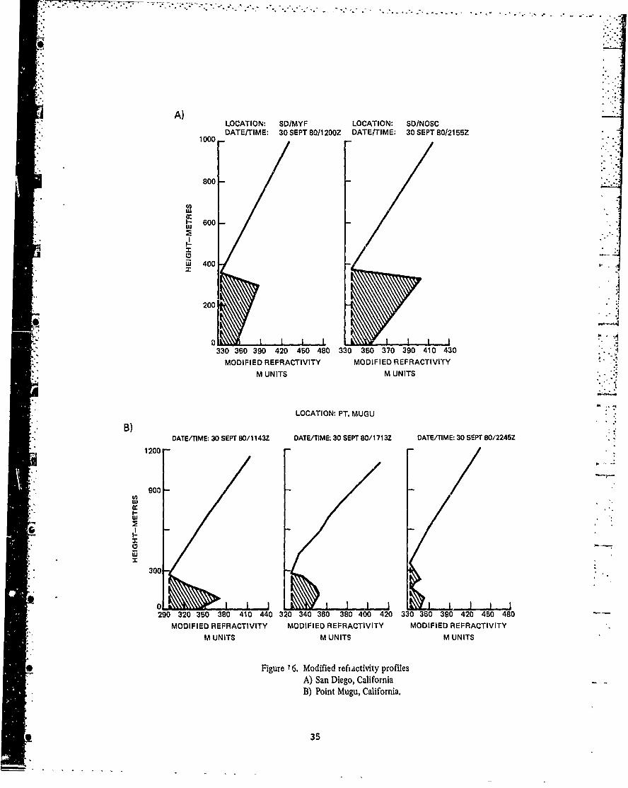
The propagation conditions occurring during *his time are shown in Figure

16. Figure 16a shows refractivity cinditons obtained in the San Diego area on

'-itember 30, 1980 at 1200 " and 2155 Z. The refractivity layer formed at an

altitude of approximacly 300 metres in the near shore region and, as can be

seen, was very stable for at least a twelve-hour period with an M-deficit of

approximately 30 M-units. Figure 16b shows refractivity profiles obtained at

Point Mugu, north of San Diego, for the same time period. In this case the

refractivity layfr, also formed around 300 metres, was more variable, but

nevertheless persisted over the full twelve-hour time period. The M-deficit

for Point Hunu varied from a value in exces of 40 M-units to as small as 15

43

H-units for this time period. The wind speed at surface level reported by

ships in the area varied from slight to moderate. Visual observations at NOSC

indicated moderate white cap formation. 0

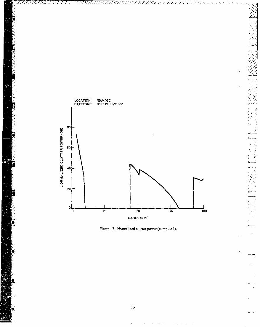
A normalized sea clutter power versus range was calculated using the

models previously discussed. An example of thene results is shown in Figure

17 for the refractivity profiles obtained at NOSC at 2155 Z. The key point to

notice is the large increase in clutter power at a range of approximately

40nmi and the second increase at a range of approximately 90 nmi. The second

increase, however, only reaches a level approximately 15 dB below the 40-nn"

results. The clutter power results presented irn Figure 17 are quite typical

of the results obtained for the profiles persisting throughout the time period

prebanted in Figure 16. .

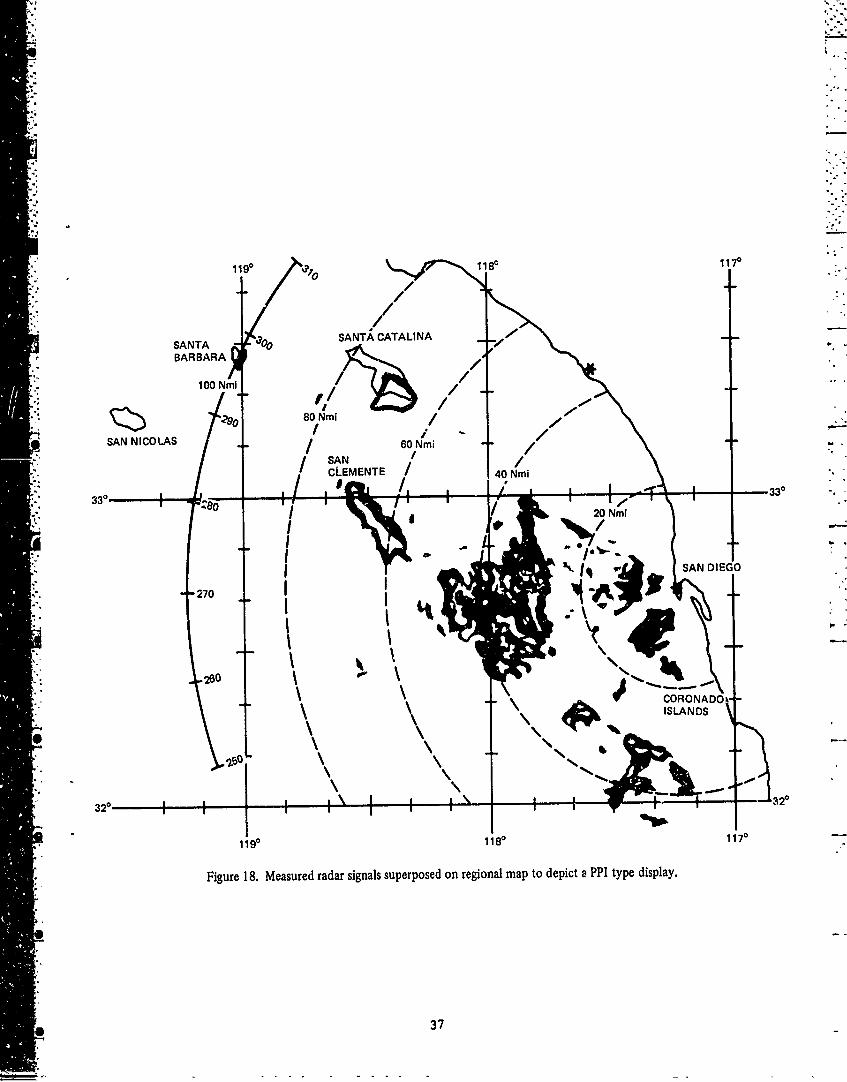
Radar backscatter signals averaged over a two-minute period were recorded

at approximately 30-'minute intervals during the same time period of Figure

16. Results obtained for a short period between 2000 Z and 2300 Z are shown

in Figure 18. The presentation in Figure 18 shows essentially a tracing of

what would be displayed on a PPI radar scope, superimposed on a map cof the

geographic area. Note the darkened outline around San Clemente Island. This

represents the large signals returned from the island. The signals returned

from very large distances, such as from Santa Barbara Island, which is

approximately 100 nmi from the radar, indicates the generally extensive -

persistence of the surface based ducting region which occurred during this

time period. Because only limited angular sectors could be examined at any

given time with the data acquisition system, not all angular sectors are

included in this time period. For those sectors which are included there is

generally a significant signal return from the 30- to 50-nmi range, which is

consistent with the model predictions. The relative signal strengths from the

-- m 2../ •

various sectors differed considerably, by as much as 15 to 20 dB. Because

each sector was sampled at different times, these variations are possibly -.

caused by spatial and temporal variations in refractivity and wind speed.

A major requirement in the validation of the clutter model is the avail-

ability of the clutter return absolute amplitude. The measurement of appro-

priate voltages along the radar input circuits while using a calibrated input

at the antenna was not possible due to radar use limitations. The calibration

procedure used employed a small calibrated tsrget (of known cross section)

being towed radially away from the radar site. The target was mounted on a

2.5-metre mast, made of pleastic sewer pipe, and the mast was mounted on a,

small rubber raft using all nonconducting materials. The raft and mast ar- ._

rangement was then towed at slow speed (5 kts) using an 800-foot tow line. In

the intervening time between the acquisition of the September 30, 1980 data

and the calibration data, numerous modifications were made in the SPS-10 radar

by ICSTF technicians. Included were changes in the antenna feeds as well as

numerous electronic components within the radar proper. Because of this,

absolute calibration for the September 1980 data is unavailable.

25

CONCLUSIONS AND RECOMMENDATIONS

A radar sea clutter model based on a ray-optics propagation formulation

combined with a semi-empirical normalized sea clutter radar cross-section has

been presented. A preliminary form of the model was coded in FORTRAN for

incorporation into the IREPS. The model was exercised for typical propagation

conditions and found to be in agreement with what limited observation data are

available. A single frequency, single location validation effort was conduct-

ed. Model and observed results were in agre6ment, although absolute amplitude

data were not obtained. 0

A multifrequency and multilocation validation effort should be conducted

using dedicated equipments. The locations should be selected to optimize the

occurrence of ducted propagation and significant sea clutter return.

Incorporation of clutter models into IREPS should be done only after a

successful validation effort.

26S

* . * . * * , *

"CYLINDRICAL CARTESIANSCOORDINATE FRAME COORDINATE FRAME

REFRACTIVE , REFRACTIVE"INDEX - n(p) INDEX - n(z)exp(z/a)

z .. V(x, z)

a a+h p A00 x

x = aoz = aln(p/a)

Figure 1. Transformation from cylindrical coordinateframe to Cartesian coordinate frame. -

M-PROFILE (D)

C' (C

B1

= I I A' "S I I tI I a-

A- 1(B]CB

DISTANCE

Figure 2. Sample ray paths with a surface based duct.

S27

20 kt-

0 * -

10 /000oU) 00001 / /0 0f

w

10.

20

-40 P..0 5 10 15 20

* ~GRAZING ANGLE (MILLIRADIANS)

Figure 3. Normalized sea clutter cross-section (relative dB) vsgrazing angle (1300 MHz; - - -5600 MHz).

28

9: " "" *"-"- "-- "" "" " '" ' -' "" '- . .. ' - ' " "-- " " - " -

50K .

I- 40K - FREQUENCY 6600 MHZw "FSR 100 NM

,.. L 30Kz -i. % TARGET:pI-. '% SMALL ROCKET

Sz ~~20K !"-

., 10 KNOT WINDw

10K -%

0

0 so"-

Figure 4. Coverage dhitgram for hypothetical C-band radar -standard (non ducted) atmosphere.

"50K -

I-40Ku~mUJ30K ,.•.w FREQUENCY~s 10 N 600 M|I.Z

-- "• TARGET:20K SMALL ROCKET

". • 1K •. 10 KNOT WIND

10(

150

RANGE IN NAUTICAL MILES

Figure 5. Coverage diagram for hypothetical C-band radar -surface based duct. Duct height - 300 metres; refractive

layer thickness - 30 metres. "

50K -. ...

J P" 40K "- 4K -- FREQUENCY 5600 MHZ

U " . FSR 100 NM

" 30K --S %%S • TARGET:

I- KSMALL ROCKET

x1 20K

,'w '% 15 KNOT Wa 4 D

z10K

/[ 00 50 •,

100 ••,

150

RANGE IN NAUTICAL MILES

Figure 6. Coverage diagram for hypothetical C-band radar -surface based duct. Duct height - 300 metres; refractivelayer thickness - 30 metres.

•, 29

Lww

I- -~% -LAYER

2 I ~ THICKNESS -

VARIABLE SLOPE LAE A m10HEIGHT - .118

Ah0

75 sws

X 300

100 2m =oo x0pm s

* z

W 500

25I25

24060 5 8 10 0 15 20 1416LAERTHCKESS(MTRE

~~~~Figure 8. ChneiRange to clutter rings vslyrtikesfr-andou cluater reigturand -eii

30- 00

.- S

A3 PROTOTYPE dM

-Z- ;dZ A 1 <Z<Z2

- dM

A- - -- Z 2 Z 2 < z<Z 3

A A1 Z dMZI dYZ" 3 Z3 < Z

-- =•M3 M1 M2

SA2 - A, A, Z < Z2

(A) dZ A + e..(Z -Z 2 )/H A2 Z> Z2

dM N Ai - Aj-1 Ai; Zj; KNOWN(B) ; Z- A , + T , -(Z - i

.j2 1 + e '(Z -Z1)/H1 Hj; SELECTED

N I/ +e (z -z 1)/Hj1.(C) M - M(Z1 ) + (Z-Z)IA 1+ (Ai-Aj. 1 ) Hj.I Ln

"j,2 + e (ZI - ZJ)/Hj-1]

Figure 9. Development of analytic profile for ray trace.

1000. -

K HEIGHT MVALUE DM/DZ DZ

1 0.0 350.0 800. -

2 300.0 440.0 0.300 300.0

3 350.0 320.0 -2tADO 50.0

4 450.0 331.8 0.118 100.0* 600.

5 550.0 343.8 0.118 100.0

INPUT TURNING POINT SMOOTHING HEIGHTS

1 H-SCALE - 20: 5:2 H-SCALE -. 20:5: - 400.

3 H-SCALE - 20: 5:

200.

0.300. 350. 400. 450. 500.

Figure 10. Sample of analytic profile generation.

31

_ --. R -I P

400.

-400. UNPERTURBED

• / WAVELENGTH: 10KM••""-"'400. AMPLITUDE: 10M

-•-.HEIGHT: 300M

300.

.I-

_• 200.

*1 w

100.

• ~~0. .J

S0 50 10O0 150 200 250WARANGEL(KM)

[ Figure I Ia. Sample effect of periodic elevated layer.

400.A UNPERTURBED

300. -

w 200.

w100.

S0. .

WAVELENGTH: 2KM400. AMPLITUDE: 1%/2m

400. FHEIGHT: 20m300.

200.

w

100.

0.

0 50 100 150 200 250SWRANGEL(KM)Figure 11 b. Sample effect of periodic evaporation layer.

32

77

TXf

SIF

SPALIS/ATEPRAYDAASTRPA CQR C O N R O L E

CASETE TOAG

PULS RATE 2O

50 4. ANGL EA

9 • " L AMP

-•-'-" ' TRIGGER ! ""'i • ~~DIGITAL SYNCRO INFORMATION|- ";'" ~D/A "'

:•'" ~TEMPORARY DATA STOR. .,,S~~ACO CONTROLLER,,

CASSETTE STORAGE

2FREQ: 560 MHZ 63BAND)PULSE RATE:ý 325 ppi

RMAX RANGE: 240 KM

n • - Figure 12. Modifications to SPS-IO0 radar. .

50 .4 .3 .2 .1 .05 0 GRAZING ANGLE

25 -- A: 6.3°

S~RANGECELL: .97 NM

j00 I I I

0 5 10 15 20

•> 50 ".•OxSECTOR: 600

w 35a 25 .s

n- 25 RANGE

CELL: .32 NM

0I I I I

0 5 10 15 20RANGE (NM)

DATE: 1/18/80

WIND SPEED: 15 KTS - GUSTS TO 20 KTS

Figure 13. Sample signals with nonducted propagation.

6 33

* -, SECTORS: 1070 AND 67.50

"A: 9.8 - 4.2

RANGE

CELL: .97 - .73

25

0 25 50 75 100

"RANGE (NM)

DATE: 4/16/80

WIND SPEED: LESSTHAN5KTS

--* Figure 14. Sample signals with ducted propagation. -

• LOS ANGELES

0N

Fiue," apo SCLOPAE deitngrdr"eun

Qto SANTA CATALINASSAN NICOLAS ý5m/1 M ,,,

•, C/1 M

•--•" , SAN CLEMENTE • . •,SAN DIEGO

-" 5m/lm ,5m/lm

S~Figure 15. Map of SOCAL OP-AREA depicting radar return.

34

S~~A) ""

LOCATION: SD/MYF LOCATION: SD/NOSCDATE/TIME: 30 SEPT 80/1200Z DATE/TIME: 30 SEPT 80/2155Z

"1000

800

LU

- 600

r 400

200

330 360 390 420 450 480 330 350 370 390 410 430

"MODIFIED REFRACTIVITY MODIFIED REFRACTIVITY

M UNITS M UNITS

LOCATION: PT. MUGU

DATE/TIME: 30 SEPT 80/1143Z DATE/TIME: 30 SEPT 80/1713Z DATE/TIME: 30 SEPT 80/2245Z

1200

900 -

_300

0 ° -

290 320 350 380 410 440 320 340 360 380 400 420 330 360 390 420 450 480

MODIFIED REFRACTIVITY MODIFIED REFRACTIVITY MODIFIED REFRACTIVITY %

M UNITS M UNITS M UNITS

* Figure '6. Modified refiactivity profilesA) San Diego, CaliforniaB) Point Mugu, California.

"35

LOCATION: SD/NOSCDATE/TIME: 30 SEPT 80/2155Z

. <. ,80

o -SMw

2~0 -

C.

C 40 -

W 0

20

0 25 50 75 100

RANGE (NMI)

Figure 17. Normalized clutter power (computed).

36

1190 17

SATA IOSANTA CATALINA 10

BARBARA 01

100 Nmi

SAN NICOLAS /60 Nmi/SANCLEMENTE /40 N4i

330 /33

IDIE

CORONADOzISLANDS

____ _______ ____ ____ ___320

320 I II I

1190 1180 17

Figure 18. Measured radar signals superposed on regional map to depict a PPI type display.

37

REFERENCES

Ament, W. S., "Toward a theory of reflection by a rough surface," Proc. IPE.,"41, No. 1, 142-146, January 1953

Beard, C. I., "Coherent and incoherent scattering of microwaves; from theocean," IRE Trans., Vol. AP-9, September 1961.

Booker, H. G., "Fitting of multi-region ionospheric profiles of electrondensity by a single analytic function of height," Jour. Atmos. Terr.Phys., Vol. 39, pp 619-623, 1977.

Hattan, C. P., "Propagation models for IREPS revision 2.0," NOSC TR 77:, April"1982.

Hitney, H. V., R. A. Paulus, C. P. Hattan, K. D. Anderson, G. E. Lindem,"IREPS revision 2.0 user's manual," NOSC TD 481, September 1981.

Jones, D. S., Methods in Electromagnetic Wave Propagation, Clarendon Press,Oxford, 1979.

Kerr, D. E. (ed.), "Propagation of short radio waves," MIT RadiationLaboratory Series, Vol. 13, McGraw-Hill, New York, 1951.

Richter, J. H,, "Application of conformal mapping to earth-flatteningprocedures ia radio propagation problems," Radio Science, Vol. 1, No. 12,December 1966, pp. 1435-1438.

Snyder, F. P., "Radar clutter under atmospheric ducting conditions,"Proceedings of the Atmospheric Refractivity Effects AssessmentConference, 23-25 January 1979, San Diego, CA. NOSC TD 260, pp 61-67.

p

Trebits, B., M. Horst, M. Long, N. Currie and J. Peifer, "Millimeter Radar SeaReturn Study," Georgia Institute of Technology, Project A-2013, InterimReport, July 1978.

3

0 39