in copyright - non-commercial use permitted rights ...29242/... · diss. eth no. 16801...
TRANSCRIPT

Research Collection
Doctoral Thesis
Collisionless and collisional dynamics in astrophysics
Author(s): Zemp, Marcel
Publication Date: 2006
Permanent Link: https://doi.org/10.3929/ethz-a-005306648
Rights / License: In Copyright - Non-Commercial Use Permitted
This page was generated automatically upon download from the ETH Zurich Research Collection. For moreinformation please consult the Terms of use.
ETH Library

DISS. ETH NO. 16801
Collisionless and CollisionalDynamics in Astrophysics
A dissertation submitted to
ETH Zurich
for the degree of
Doctor of Sciences
presented by
Marcel Zemp
Dipl. phys. ETH Zurich
born June 7, 1977
citizen of
Risch (ZG) and Escholzmatt (LU)
accepted on the recommendation of
Prof. Dr. C. Marcella Carollo, examiner
Prof. Dr. Ben Moore, co-examiner
Prof. Dr. George Lake, co-examiner
2006

ii

Contents
Kurzfassung ix
Abstract xi
1 General introduction 11.1 Overwiew . . . . . . . . . . . . . . . . . . . . . . . . . . . . . . . . . . . 11.2 Self-gravitating systems . . . . . . . . . . . . . . . . . . . . . . . . . . . 2
1.2.1 Long range nature of gravity . . . . . . . . . . . . . . . . . . . . . 21.2.2 Equations of motion . . . . . . . . . . . . . . . . . . . . . . . . . 21.2.3 Collisionless versus collisional . . . . . . . . . . . . . . . . . . . . 31.2.4 Distribution function and Boltzmann equations . . . . . . . . . . 4
1.3 Numerical methods . . . . . . . . . . . . . . . . . . . . . . . . . . . . . . 51.3.1 Monte-Carlo methods . . . . . . . . . . . . . . . . . . . . . . . . . 51.3.2 Dynamical evolution and symplectic integrators . . . . . . . . . . 71.3.3 Choice of time-steps . . . . . . . . . . . . . . . . . . . . . . . . . 81.3.4 Acceleration calculation . . . . . . . . . . . . . . . . . . . . . . . 81.3.5 PKDGRAV . . . . . . . . . . . . . . . . . . . . . . . . . . . . . . 15
1.4 Unifying both regimes . . . . . . . . . . . . . . . . . . . . . . . . . . . . 161.5 Content of this thesis . . . . . . . . . . . . . . . . . . . . . . . . . . . . . 18
2 Multi-mass halo models 212.1 Introduction and motivation . . . . . . . . . . . . . . . . . . . . . . . . . 212.2 Method . . . . . . . . . . . . . . . . . . . . . . . . . . . . . . . . . . . . 232.3 Tests . . . . . . . . . . . . . . . . . . . . . . . . . . . . . . . . . . . . . . 25
2.3.1 Two-shell models . . . . . . . . . . . . . . . . . . . . . . . . . . . 252.3.2 Three-shell models . . . . . . . . . . . . . . . . . . . . . . . . . . 30
2.4 Preservation of cusp slope . . . . . . . . . . . . . . . . . . . . . . . . . . 322.5 Conclusions . . . . . . . . . . . . . . . . . . . . . . . . . . . . . . . . . . 35
3 An optimum time-stepping scheme 373.1 Introduction . . . . . . . . . . . . . . . . . . . . . . . . . . . . . . . . . . 373.2 Dynamical time-stepping . . . . . . . . . . . . . . . . . . . . . . . . . . . 38
3.2.1 General idea and description . . . . . . . . . . . . . . . . . . . . . 383.2.2 Implementation within a tree-code . . . . . . . . . . . . . . . . . 39
3.3 Time-stepping criterion tests and behaviour . . . . . . . . . . . . . . . . 443.3.1 General properties . . . . . . . . . . . . . . . . . . . . . . . . . . 443.3.2 Elliptic 2-body orbits . . . . . . . . . . . . . . . . . . . . . . . . . 48
iii

Contents
3.3.3 Hyperbolic 2-body orbits . . . . . . . . . . . . . . . . . . . . . . . 523.3.4 Cosmological structure formation . . . . . . . . . . . . . . . . . . 543.3.5 Dependence on parameters . . . . . . . . . . . . . . . . . . . . . . 563.3.6 Efficiency . . . . . . . . . . . . . . . . . . . . . . . . . . . . . . . 57
3.4 Conclusions . . . . . . . . . . . . . . . . . . . . . . . . . . . . . . . . . . 61
4 Applications 654.1 Cusps in cold dark matter haloes . . . . . . . . . . . . . . . . . . . . . . 65
4.1.1 Introduction . . . . . . . . . . . . . . . . . . . . . . . . . . . . . . 654.1.2 Numerical methods . . . . . . . . . . . . . . . . . . . . . . . . . . 674.1.3 Results . . . . . . . . . . . . . . . . . . . . . . . . . . . . . . . . . 68
4.2 Does the Fornax dwarf spheroidal have a central cusp or core? . . . . . . 744.2.1 Introduction . . . . . . . . . . . . . . . . . . . . . . . . . . . . . . 744.2.2 Numerical methods . . . . . . . . . . . . . . . . . . . . . . . . . . 754.2.3 Results . . . . . . . . . . . . . . . . . . . . . . . . . . . . . . . . . 76
5 Summary and perspective 81
Appendix 85
A Hamiltonian formalism 87
B Further projects 91B.1 A universal velocity distribution of relaxed collisionless structures . . . . 91
B.1.1 Introduction . . . . . . . . . . . . . . . . . . . . . . . . . . . . . . 91B.1.2 Numerical methods and results . . . . . . . . . . . . . . . . . . . 91
B.2 Globular clusters, satellite galaxies and stellar haloes from early darkmatter peaks . . . . . . . . . . . . . . . . . . . . . . . . . . . . . . . . . 95B.2.1 Introduction . . . . . . . . . . . . . . . . . . . . . . . . . . . . . . 95B.2.2 The first stellar systems . . . . . . . . . . . . . . . . . . . . . . . 96B.2.3 Connection to globular clusters and halo stars . . . . . . . . . . . 98B.2.4 Connection to satellite galaxies and the missing satellites problem 100
Bibliography 103
Curriculum vitae 119
Publications 121
Acknowledgment 123
iv

List of Figures
1.1 Comparison of a symplectic and a non-symplectic integrator . . . . . . . 91.2 Compensating softening kernels . . . . . . . . . . . . . . . . . . . . . . . 121.3 Geometrical configuration for multipole expansion . . . . . . . . . . . . . 131.4 Quad-tree . . . . . . . . . . . . . . . . . . . . . . . . . . . . . . . . . . . 151.5 Positions and orbital fits for seven stars in the Galactic centre . . . . . . 17
2.1 Mean particle separation function . . . . . . . . . . . . . . . . . . . . . . 222.2 Multi-mass stability tests: density profiles . . . . . . . . . . . . . . . . . 262.3 Multi-mass stability tests: anisotropy profiles . . . . . . . . . . . . . . . . 282.4 Computer run time versus mass ratio . . . . . . . . . . . . . . . . . . . . 292.5 Three-shell multi-mass model . . . . . . . . . . . . . . . . . . . . . . . . 312.6 Equal profile mergers after 10 Gyr . . . . . . . . . . . . . . . . . . . . . . 332.7 Cusp-core merger after 10 Gyr . . . . . . . . . . . . . . . . . . . . . . . . 34
3.1 Viewing cone for add-up scheme . . . . . . . . . . . . . . . . . . . . . . . 423.2 Time-step distribution for different density profiles . . . . . . . . . . . . . 463.3 2-body orbits with different eccentricities . . . . . . . . . . . . . . . . . . 493.4 2-body orbits with eccentricity e = 0.9 . . . . . . . . . . . . . . . . . . . 503.5 Orbit of run p) . . . . . . . . . . . . . . . . . . . . . . . . . . . . . . . . 513.6 Orbit of run I) . . . . . . . . . . . . . . . . . . . . . . . . . . . . . . . . . 523.7 Orbits of run J) and K) . . . . . . . . . . . . . . . . . . . . . . . . . . . 533.8 Virgo cluster: density profiles . . . . . . . . . . . . . . . . . . . . . . . . 553.9 Virgo cluster: substructure mass function . . . . . . . . . . . . . . . . . . 563.10 Number of force evaluations . . . . . . . . . . . . . . . . . . . . . . . . . 59
4.1 Logarithmic slope of the density profile of run DM25 . . . . . . . . . . . 694.2 Logarithmic slope of the density profile of run D5, DM25 and DM50 . . . 704.3 Density profiles in physical coordinates . . . . . . . . . . . . . . . . . . . 724.4 Logarithmic slope of the extrapolated DM50 density profile . . . . . . . . 734.5 Radial distance of a single globular cluster from the centre of its host halo 774.6 Globular clusters in cuspy halo . . . . . . . . . . . . . . . . . . . . . . . 794.7 Globular clusters in cored halo . . . . . . . . . . . . . . . . . . . . . . . . 80
B.1 Radial velocity distribution function . . . . . . . . . . . . . . . . . . . . . 93B.2 Tangential velocity distribution function . . . . . . . . . . . . . . . . . . 94B.3 Galaxy at redshift z = 12 and z = 0 . . . . . . . . . . . . . . . . . . . . . 97
v

List of Figures
B.4 Radial distribution of old stellar systems compared with rare peaks withina z = 0 ΛCDM galaxy . . . . . . . . . . . . . . . . . . . . . . . . . . . . 99
vi

List of Tables
2.1 Summary of parameters for the different models . . . . . . . . . . . . . . 272.2 Summary of parameters for the two initial conditions used for the mergers 32
3.1 Number of force evaluations . . . . . . . . . . . . . . . . . . . . . . . . . 603.2 Summary of elliptic 2-body orbit runs a) - p) . . . . . . . . . . . . . . . . 623.3 Summary of hyperbolic 2-body orbit runs A) - K) . . . . . . . . . . . . . 63
4.1 Summary of cluster models . . . . . . . . . . . . . . . . . . . . . . . . . . 67
vii

List of Tables
viii

Kurzfassung
In dieser Doktorarbeit werden Methoden entwickelt, um astrophysikalische Prozesse zustudieren, welche Dynamik mit und ohne Kollisionen beinhaltet. Die Hauptanwendung,fur die diese Methoden entwickelt wurden, ist das Studium von dynamischen Effekten,die bei Galaxien-Verschmelzungen mit super-massiven Schwarzen Lochern in den Zen-tren der jeweiligen Galaxien entstehen. Dies ist eine schwierige Problemstellung ummit N-body Methoden zu untersuchen, denn es enthalt sowohl kollisionsfreie Dynamikals auch Dynamik mit Kollisionen. Ebenso mussen ein enormer Bereich in Raum undZeit aufgelost werden, um die wahren physikalischen Effekte zu sehen wenn man nichtnumerischen Artefakten wie Relaxation in N-body Simulationen erliegen will.
In einer allgemeinen Einleitung 1 werden zuerst die physikalischen Grundlagen vonselbst-gravitierenden Systemen diskutiert und eine kleine Ubersicht uber die heutzutageverwendeten numerischen Methoden gegeben.
In Kapitel 2 wird eine simple Methode (Multi-Massen-Technik) prasentiert, um Mod-elle von Halo-Profilen mit verschiedenen Massen und Auflosung zu generieren. Mitdieser Methode wird die Computer Laufzeit in Simulationen gegenuber Modellen mitnur einer fixen Auflosung drastisch reduziert. Dies erlaubt bei einer gegebenen Com-puter Laufzeit viel kleinere Skalen zu untersuchen. Als Anwendung bestatigen wir dieAussage von Dehnen [31], dass in Verschmelzungen von dunkle Materie Halos immer dassteilste zentrale Profil eines Vorgangers erhalten bleibt. Fur diese Anwendung werdenhoch auflosende N-body Simulationen benotigt, wobei wir jeden in der Verschmelzungbeteiligten Vorganger mit ungefahr 5× 10⁷ Teilchen auflosen.
Als eine bedeutende neue Entwicklung wird in Kapitel 3 ein Zeit-Schritt Kriterium furN-body Simulationen prasentiert, das auf der wahren dynamischen Zeit eines Teilchensbasiert. Dieses Kriterium erlaubt der jeweiligen Bahn eines Teilchens in allen Umgebun-gen korrekt zu folgen, da das Kriterium eine bessere Anpassungsfahigkeit als vorherigeKriterien hat. Zusatzlich wird eine kleinere Anzahl von Berechungen der Kraft in Re-gionen mit einer kleineren Dichte benotigt und die Methode hangt nicht direkt vonartifiziellen Parametern wie zum Beispiel der Softening-Lange ab. Daher kann dieseMethode mehrere Grossenordnungen schneller sein als konventionellen Methoden, welchezum Beispiel eine Kombination von Beschleunigung und Softening-Lange als Kriteriumbenutzen. Das neue Kriterium ist daher ideal um schwierige Probleme zu losen, wie zumBeispiel die Dynamik in Zentren von dunklen Materie Halos zu studieren. Ebenso wirdeine Exzentrizitatskorrektur fur ein Leapfrog Integrationsschema hergeleitet, welches er-laubt Zweikorperinteraktionen mit Exzentrizitat e → 1 mit grosser Prazision zu ver-folgen. Diese Neuentwicklung erlaubt es, einen grossen Bereich von Problemen zustudieren, welche Kollisionen enthalten als auch kollisionsfrei sind. Es werden Testsdieses neuen Schemas in N-body Simulationen von Zweikorperproblemen mit Exzen-
ix

Kurzfassung
trizitat e → 1 (elliptisch und hyperbolisch), Gleichgewichts-Halo-Profilen und von kos-mologischen Strukturbildungs-Simulationen prasentiert.
In Kapitel 4 werden die ersten Anwendungen dieser Neuentwicklungen prasentiert. Inder ersten Anwendung wurde die Multi-Massen-Technik dazu verwendet in einer kosmol-ogischen Simulation das Dichteprofil eines Galaxienhaufens bis runter zu einem Promilledes virial Radius zu bestimmen. Das innere Profile des Galaxienhaufens wird gut durchein Potenzgesetz der Form ρ(r) ∝ r−γ beschrieben wobei γ = 1.2. Eine weitere An-wendung der Multi-Massen-Technik war der Test einer potentiellen Erklarung fur diePosition von funf Globular Clusters bei der ungefahren Distanz von 1 kpc vom Zentrumder Zwerggalaxie Fornax. In einer Kosmologie mit dunkler Materie und dunkler Energieals Hauptbestandteile wurden diese Globular Clusters innerhalb von ein paar MilliardenJahren von der heutigen Position ins Zentrum sinken. Eine mogliche Losung hierfurware, dass das dunkle Materie Halo der Fornax Zwerggalaxie einen Kern mit konstanterDichte hat, denn in einem Kern konstanter Dichte wird die Zeit, die fur ein Sinken zumZentrum benotigt wird, viel langer als die Hubble-Zeit und die Globular Clusters bleibenbeim Kernradius stehen. Um diese Hypothese zu testen waren hoch auflosende Modellevon dunkle Materie Halos notig.
Zum Schluss wird eine Zusammenfassung prasentiert und ein Ausblick auf weitereProjekte in der Zukunft gegeben.
x

Abstract
This thesis develops numerical methods in order to study astrophysical processes thatinclude collisionless and collisional dynamics. As a major application that involves suchprocesses, the dynamical effects of merging galaxies with super-massive black holes intheir centres were in mind when these methods were developed. This is a very difficultproblem to simulate with N-body methods since it demands a combination of collisionlessand collisional dynamics. It also involves an enormous spatial and temporal range inorder to observe the real physical effects and not suffer from numerical artefacts likerelaxation in the N-body simulations.
In a general introduction 1, we first discuss the basic physics of self-gravitating systemsand present a short overview of some of the numerical methods used in the field ofcomputational astrophysics today.
We then present in chapter 2 a simple way to model halo profiles with a multi-masstechnique. This technique reduces the computer run time that would be needed bya single-mass model resolving the same scales by several factors and therefore allowsto resolve smaller scales in N-body simulations for a given computer run time. As anapplication, we test and confirm the prediction by Dehnen [31], that in mergers of darkmatter haloes always the cusp of the steepest progenitor of the merger is preserved. Thisapplication required high resolution N-body simulations where we model each mergerprogenitor with an effective number of particles of approximately 5× 10⁷ particles.
As a major new development, we present in chapter 3 a new time-stepping criterionfor N-body simulations that is based on the true dynamical time of a particle. Thisallows us to follow the orbits of particles correctly in all environments since it has betteradaptivity than previous time-stepping criteria used in N-body simulations. Further-more, it requires far fewer force evaluations in low density regions of the simulation andhas no dependence on artificial parameters such as, for example, the softening length.This can be orders of magnitude faster than conventional ad-hoc methods that employcombinations of acceleration and softening and is ideally suited for hard problems, suchas obtaining the correct dynamics in the very central regions of dark matter haloes.We also derive an eccentricity correction for a general leapfrog integration scheme thatcan follow gravitational scattering events for orbits with eccentricity e → 1 with highprecision. These new approaches allow us to study a range of problems in collisionlessand collisional dynamics from few-body problems to cosmological structure formation.We present tests of the time-stepping scheme in N-body simulations of 2-body orbitswith eccentricity e → 1 (elliptic and hyperbolic), equilibrium haloes and a hierarchicalcosmological structure formation run.
In chapter 4, we present the first applications of these new developments that alreadyled to new insights and physical results. In one application, the multi-mass technique
xi

Abstract
was used in a cosmological structure formation run in order to resolve the resultingdensity profile of a high resolution cluster down to one per mill of the virial radius. Theinner density profile of this cluster halo is well fit by a power law ρ(r) ∝ r−γ down to thesmallest resolved scale with γ = 1.2. This means that the dark matter profiles still obeya power law scaling down to one per mill of the virial radius. Another application of themulti-mass models was to test a potential explanation of the presence of the five globularclusters at approximately 1 kpc distance from the centre of the Fornax dwarf spheroidalgalaxy. In a cuspy cold dark matter halo as predicted from large scale structure formationsimulations in a lambda cold dark matter (ΛCDM) cosmology, the globulars would sinkto the centre from their current positions within a few Gyr, presenting a puzzle as towhy they survive at their present positions. A possible solution to this timing problemis to adopt a cored dark matter halo for the Fornax dwarf spheroidal. In a cored darkmatter halo, the sinking time becomes many Hubble times and the globular clusterseffectively stall at the dark matter core radius. In order to perform these simulationsand test this hypothesis, high resolution multi-mass models were needed to obtain therequired spatial resolution.
Finally, we summarise and give a perspective on future projects in chapter 5.
xii
Chapter 1
General introduction
1.1 Overwiew
In astrophysics, a variety of self-gravitating systems exist. Such systems range fromthe Keplerian 2-body system, the stability of the solar system, core collapse in globularclusters, galaxy mergers up to the formation process of large scale structure in theuniverse. Computational methods like N-body simulations are a powerful tool to studysuch self-gravitating systems. The ultimate goal would be to study the evolution of theuniverse from early initial conditions after the big bang until the present with all therelevant physics involved but the available computer resources have so far allowed onlythe study of certain aspects of the full picture.
Hence, two communities emerged out of this. The first concentrated on small as-trophysical systems like star clusters where time-scales are short and the dynamics ofthe system is mainly collisional. In contrast, the long-term and large scale structureformation, that is governed by the dynamical evolution of collisionless dark matter par-ticles, is the working field of the other community. Both communities developed theirown methods and specific techniques in order to treat the individual numerical problemsoptimally.
But many systems in astrophysics can not be fully described by only one regime. Forexample, the dynamics of super-massive black holes in the centre of a galaxy-galaxymerger remnant is dominated by collisional dynamics whereas the large scale shape ofthe resulting structure is a result of the collisionless dynamics of the dark matter. Withthe ever increasing computer resources, a combination of these two regimes becomesfeasible. This thesis project had therefore the aim to develop the numerical techniquesin order to perform N-body simulations that include collisionless as well as collisionaldynamics.
This chapter gives the reader an introduction to the basic physics of self-gravitatingsystems and a short overview of some of the numerical methods used in the field of com-putational astrophysics today. A more detailed motivation for combining the collisionlessand collisional regime is given towards the end of the introduction.
1

Chapter 1 General introduction
1.2 Self-gravitating systems
1.2.1 Long range nature of gravity
The nature of the gravity force makes a self-gravitating system behave completely differ-ent than for example a neutral gas. Generally, the electromagnetic forces between twogas molecules are small since the gas is neutral on large scales. As a consequence themolecules move at nearly constant speed for long periods until they collide with anothermolecule where they feel a strong acceleration due to the close interaction. Thus, onlyforces on short length scales that arise from collisions are important and we can neglectlong range forces since the gas is neutral and the two different electromagnetic chargescompensate on these scales.
In contrast, gravity is always attractive since there is only one charge in gravity; thereis only positive mass as far as we know. Let’s consider a homogeneous system withdensity ρ. The force from a cone segment on a particle at its apex with mass dmC atdistance r with thickness dr and solid angle dΩ around the particle is given by
dmC = ρr2drdΩ . (1.1)
Therefore, the contribution from this cone segment to the total force on that particleresults in
dF = Gm dmC
r2= GmρdrdΩ . (1.2)
For a homogeneous system, the force per unit length dF/dr from that cone segmentis therefore independent of radius and force contributions arising from all scales areimportant. Of course, if the system is perfectly spherical around the particle and ho-mogeneous, no net force will act on the particle. But inhomogeneities on all scales canresult in a net force on any particle.
1.2.2 Equations of motion
Let’s assume a self-gravitating system is described by a smooth distribution of massgiven by the density ρ(x ′, t) and our goal is to calculate the acceleration on a particleat a position x . By Newton’s inverse-square law, we can express the total accelerationby integrating over the whole volume and obtain
a(x , t) = G
∫x ′ − x
|x ′ − x |3ρ(x ′, t)d3x ′ . (1.3)
Here, G is Newton’s constant of gravity. We can define a scalar function Φ(x , t) by
Φ(x , t) ≡ −G
∫ρ(x ′, t)|x ′ − x |d
3x ′ . (1.4)
This function Φ(x , t) is called the gravitational potential and with
∇(
1
|x ′ − x |)
=x ′ − x
|x ′ − x |3 , (1.5)
2

1.2 Self-gravitating systems
we finda(x , t) = −∇Φ(x , t) . (1.6)
Here, the gradient operator ∇ is always meant with respect to x .With
∇(
x ′ − x
|x ′ − x |3)
= ∇2
(1
|x ′ − x |)
= −4πδ(x ′ − x ) , (1.7)
where δ(x ′ − x ) is the Dirac delta-function we can now write
∇a(x , t) = G
∫(−4πδ(x ′ − x )) ρ(x ′, t)d3x ′ = −4πGρ(x , t) . (1.8)
By substituting from equation (1.6), we get the Poisson equation
∇2Φ(x , t) = 4πGρ(x , t) . (1.9)
The equations of motion are now given by
x (x , t) = v(x , t) (1.10)
x (x , t) = v(x , t) = a(x , t) = −∇Φ(x , t) (1.11)
∇2Φ(x , t) = 4πGρ(x , t) . (1.12)
In order to calculate the trajectory x (t) of the particle, this system of coupled second-order differential equations in space and time has to be solved. Generally, this can onlybe solved with numerical methods for an arbitrary configuration ρ(x , t).
1.2.3 Collisionless versus collisional
Of course, real astrophysical systems are not perfectly smooth but they consist of discreteparticles like stars, black holes or dark matter particles that mutually interact via gravity.The relaxation is a measure for the effect that a particle is not moving in a smoothpotential but through a potential that is generated by the discrete configuration of theindividual particles in the system. Since each individual particle is slightly perturbedby the mutual interactions with all the other particles, its velocity will deviate from thevalue it would have in a smooth potential due to the discreteness of the system.
As a measure for the speed of this relaxation process, we define the relaxation timeTrelax by the time where the change of the velocity is of order of the velocity itself, whichresults in
Trelax =N
8 ln ΛTcross , (1.13)
where Tcross is the crossing time needed for the particle to cross the system and
ln Λ ≡ ln
(bmax
bmin
)(1.14)
is called the Coulomb logarithm and bmax respectively bmin are the minimum respectivelymaximum impact parameters of the particle under consideration. Trelax is the time-scalewhere the system looses its memory of its initial state.
3

Chapter 1 General introduction
For galaxies with N ≈ 1011 stars and an age of approximately 10 Gyr (which corre-sponds to a few hundred crossing times), the relaxation time-scale for the whole systemis much longer than the age of the universe and close encounters are entirely unimpor-tant. Also for dark matter haloes relaxation is completely negligible. If dark matterconsists of neutralinos then their expected mass is of order of a few hundred GeV/c2
[44] which corresponds to a total number of N ≈ O(1067) particles within a Milky Waysize dark matter halo (1 GeV/c2 = 8.963× 10−58 M¯1).
On the other hand, for globular clusters with N ≈ 105 stars and a crossing timeof Tcross ≈ 105 yr, the relaxation process can be important over the cluster lifetime ofapproximately 10 Gyr. This is especially true in the centre of the globular cluster wherethe local relaxation time-scale is much smaller and can lead to core collapse.
In summary, self-gravitating systems with a relaxation time-scale much longer thanthe time interval of interest (which is at maximum the age of the universe) can be calledcollisionless. Systems with a (local) relaxation time of the order of the time interval ofinterest are called collisional, i.e. close particle encounters play an important role.2 Alsoif the smoothness of the potential breaks down and local fluctuations, arising from a fewparticles like e.g. super-massive black holes, dominate the dynamics, the interactionshave to be treated in the collisional regime.
1.2.4 Distribution function and Boltzmann equations
We can generalize the description of a self-gravitating system by introducing the distri-bution function or phase-space density f(x , v , t) where f(x , v , t)d3xd3v is the mass inthe phase-space volume d3xd3v at the phase-space point (x , v) at time t.
If we know the configuration at a time t0, either by ρ(x , t0) and the velocity field orby f(x , v , t0), the equations of motion allow us to calculate the state of the system atany later time. Hence, we’re interested in the flow of the points in phase-space. Wecan generalise the coordinates in phase-space by introducing a new coordinate vectorw ≡ (x , v) ≡ (w1, . . . , w6) and describe the velocity of this flow in phase-space byw = (x , v) = (v ,−∇Φ(x , t)).
In a collisionless system, this flow is mass conserving and therefore obeys a continuityequation
∂f(w , t)
∂t+
6∑i=1
∂ (f(w , t) wi)
∂wi
= 0 . (1.15)
By using Hamilton’s equations
xi =∂H(x , v , t)
∂vi
(1.16)
vi = −∂H(x , v , t)
∂xi
= −∂Φ(x , t)
∂xi
(1.17)
1M¯ stands for the mass of the Sun and is a standard mass unit in astrophysics. M¯ = 1.989×1030 kg.2Collisional does not mean real physical collisions; one should always think of close encounters here.
4

1.3 Numerical methods
where the appropriate Hamiltonian3
H(x , v , t) ≡ 1
2|v |2 + Φ(x , t) (1.18)
describes the energy per unit mass, we can write
6∑i=1
∂wi
∂wi
=3∑
i=1
(∂xi
∂xi
+∂vi
∂vi
)=
3∑i=1
(∂
∂xi
(∂H
∂vi
)− ∂
∂vi
(∂H
∂xi
))= 0 . (1.19)
Therefore, the continuity equation simplifies to
∂f(w , t)
∂t+
6∑i=1
wi∂f(w , t)
∂wi
=df(w , t)
dt= 0 . (1.20)
The above equation (1.20) is called the collisionless Boltzmann equation and it describesthe evolution of an incompressible fluid in phase-space that is evolved under a Hamilto-nian flow. The collisionless Boltzmann equation is a special case of Liouville’s theoremunder the assumption that the number of particles is large N À 1 and we can neglecttwo-particle and higher order correlations. For further details and an explicit derivationsee also Binney and Tremaine [15, chapter 8].
If collisions between particles are important in the astrophysical system under study,then the phase-space density around a particle will change and we have to modify thecollisionless Boltzmann equation (1.20) by
df(w , t)
dt=
∂f(w , t)
∂t+
6∑i=1
wi∂f(w , t)
∂wi
= Γ (f(w , t)) , (1.21)
where Γ (f(w , t)) is a collision term that describes the rate of change of f(w , t) due toparticle encounters. Equation (1.21) is called the Boltzmann equation.
1.3 Numerical methods
1.3.1 Monte-Carlo methods
A very efficient method in order to solve the Boltzmann equations (1.20) and (1.21)(depending on whether the system is collisional or collisionless) together with the Poissonequation (1.9) are Monte-Carlo methods where one represents the astrophysical systemunder study with N bodies. Monte-Carlo methods can be loosely described as statisticalsimulation methods, where statistical simulation is defined in quite general terms to be
3This form of the Hamiltonian is only correct in the collisionless regime since it neglects possible inter-actions between particles. The correct interactions can only be described in the full 6N dimensionalphase-space by the N -particle distribution function where the full Hamiltonian correctly describesthe mutual interactions between the particles. For more details see also Binney and Tremaine [15,chapter 8]
5

Chapter 1 General introduction
any method that utilizes sequences of random numbers to perform a simulation. Themethod is named after the capital of the principality Monaco that is famous for beinga centre for gambling and had its origin from research during the Manhattan project(development of the atomic bomb) of the second world war where such methods wereused for a direct simulation of the probabilistic problems concerned with random neutrondiffusion in fissile material.
The basic idea of Monte-Carlo methods can be illustrated by the following procedurethat allows to calculate π in a Monte-Carlo fashion. Imagine a square with area AS = d2
and inscribed a circle with area AC =(
d2
)2π = π
4AS. Now place N points randomly
and independent within that square. By counting the number NC which fall within thecircle, we can express π as
π = 4AC
AS
= 4NC
N(1.22)
since the probability that a point point lies in a certain area is proportional to that area.Since the points are generated randomly and independent, this process follows Poissonstatistics and the fractional error is of order 1/
√N . The big advantage in Monte-Carlo
method is that the error does not depend on the number of dimensions of the problembut only on the number of points N . Therefore this method can outperform othermethods in multi-dimensional problems.
In astrophysical systems, the real numbers of particles are up to the order of O(1067)particles for example for dark matter haloes (see also section 1.2.3). This enormousnumber is clearly not possible to simulate with any computer in the near future. Onetherefore samples the astrophysical system that is described by a distribution functionf(x , v , t) with N bodies, where N is much less than the number of constituents in thereal system, that have mass mi, position x i and velocity v i (i = 1 . . . N). In principle, thecontinuous distribution function f(x , v) is replaced with a discretised version fd(x , v)which consists of a set of Dirac delta-functions
f(x , v) → fd(x , v) =N∑
i=1
miδ(x i − x )δ(v i − v) . (1.23)
Initial conditions are set-up by treating the distribution function at a fixed time t0as a probability distribution, i.e. one selects coordinates (x , v) with a probability pro-portional to f(x , v) = f(x , v , t0). The real astrophysical system is now representedin a Monte-Carlo fashion by N bodies and this method is therefore also called N-bodytechnique.
Generally, by sampling the real astrophysical system with N bodies, the discretisedvariables give us an estimate (or expectation value) of the real, continuous variables.For example the discretised potential Φd(x ) gives us an estimate of the real, continuouspotential Φ(x ) and therefrom also an estimate of the acceleration ad(x ). The fractionalerror between the real variables and the estimated variables is of order 1/
√N .
We get from the Poisson equation (1.9) or directly from equation (1.4)
Φd(x ) = −G
N∑i=1
mi
|x i − x | (1.24)
6

1.3 Numerical methods
and the equations of motion in the N-body realisation have to be solved with the dis-cretised potential which is in this way calculated from the Poisson equation (1.9) by aMonte-Carlo sampling. The form of the potential (1.24) has the drawback that singulari-ties appear at the positions x i of the particles due to the discreteness of the system. Thisleads to large scatter in the estimate of the gravitational potential (or equivalently theacceleration) [89]. This can be cured by softening the potential and a detailed discussionof this technique is given in section 1.3.4.
1.3.2 Dynamical evolution and symplectic integrators
If the N-body system is evolved by the Hamiltonian phase-flow defined by equations(1.16) and (1.17), then this mapping preserves the structure of phase-space, i.e. itpreserves the Poincare invariants, hence phase-space volume and the orientation of thevolume described by the distribution function in phase-space. A map that preserves thestructure of phase-space is called a symplectic4 or canonical map. This can be seen inthe sense that starting with an N-body realisation at time t0 of f(x , v , t0) and evolvingthe N-body system under a symplectic map, then at any later time t > t0, the N-bodysystem is a realisation of f(x , v , t) at that time t.
Hence, it is desirable to have a numerical time integration scheme that also has thispreservation property. Such a scheme is called a symplectic integrator. It is the exactsolution to a discrete Hamiltonian N-body system that is close to the continuous systemthat is described by f(x , v , t). For example, if the Hamiltonian is time-independent sucha symplectic integrator would preserve the energy of the discrete system. This approx-imate energy of the N-body system oscillates about the true energy of the continuoussystem without any numerical dissipation. The difference between the discrete, approx-imate Hamiltonian and the continuous one can be seen as a small perturbation given bythe truncation error of the integrator, where this error term is also a Hamiltonian. Seealso appendix A for more details.
A commonly used symplectic integration scheme is the leapfrog integrator. It worksas follows: during a time-step ∆T , first the velocities are updated (kick mode) witha time step of ∆T/2 then the new positions are calculated (drift mode) using the newvelocities with a time-step of ∆T and finally the velocities are updated to the final valuesat ∆T with again a half-step of ∆T/2 but with the acceleration calculated from the newpositions. This scheme can be written as
v(t + ∆T/2) = v(t) + ∆T/2 a(t) (1.25)
x (t + ∆T ) = x (t) + ∆T v(t + ∆T/2) (1.26)
v(t + ∆T ) = v(t + ∆T/2) + ∆T/2 a(t + ∆T ) (1.27)
and is called the kick-drift-kick mode. The leapfrog scheme can also be formulated inthe drift-kick-drift mode, where one drifts fist for a half-step, then updates the velocities
4The term symplectic was first used by the mathematician Hermann Weyl in his book The classicalGroups [164]. Symplectic is the Greek adjective corresponding to the Latin word complex and alsomeans twining or plaiting together.
7

Chapter 1 General introduction
by a full step and then drifts again for a half-step. The leapfrog scheme is symplecticfor fixed time-steps ∆T . For further details see also Yoshida [171].
Figure 1.1 shows a comparison of a symplectic and a non-symplectic integrator fromQuinn et al. [128]. The figure shows the radial separation r and the radial velocity vr
of an eccentricity e = 0.5 Kepler 2-body orbit calculated by a second order leapfrogscheme and a fourth order Runge-Kutta integrator. In both integrations, 24 fix time-steps per orbit were taken and in total 16 orbits were calculated. The solid line isthe exact solution, the filled squares show the points of the leapfrog integrator and thecrosses are from the Runge-Kutta integrator. The leapfrog integrator oscillates aboutthe true solution and it remains always on a one dimensional surface which indicatesthat it is indeed conserving an energy-like quantity. That the orbit is constrained toa one dimensional surface shows that there exists an isolating integral of motion. Theorbit calculated with the Runge-Kutta scheme becomes more circular and the integratorperforms very bad given that this scheme is a fourth order integration using four timesas many force evaluation as the leapfrog scheme.
The symplectic leapfrog scheme is therefore an ideal choice to integrate discrete Hamil-tonian N-body systems since it can also be formulated in comoving coordinates as a sym-plectic integrator for cosmological structure formation simulations [128] and is relativelyeasy to implement in computer programs.
1.3.3 Choice of time-steps
The leapfrog scheme described above is only symplectic for fixed time-steps, i.e. onlyif all the particles have the same time-step in the N-body simulation. But in order tofollow the dynamics correctly in dense regions, this would mean that for all particles verysmall time-steps should be set. This is computationally very expensive and is thereforenot efficient for high resolution simulations.
A solution for this problem is to use variable time-steps for each particle. But by usingadaptive individual time-steps for each particle according to some selection criterion, thesymplectic behaviour is lost [128, 140].
Adaptive methods show significant speed-ups over fixed-step integrations for the priceof accuracy. By choosing the time-step criterion carefully and controlling the errors, wecan pass over to an approximate symplectic behaviour of the integration scheme so thatit is stable enough for time-scales that are not many orders of magnitudes longer thanthe dynamical time of the system. For a detailed discussion of time-stepping schemesand criteria see chapter 3.
1.3.4 Acceleration calculation
Softened accelerations
The form of the discrete gravitational potential of equation (1.24) has the drawback thatit is singular close to individual particles which leads to large scatter of the estimatedvariables like potential or acceleration. This can also lead to numerical problems during
8

1.3 Numerical methods
Figure 1.1: A comparison of a symplectic and a non-symplectic integrator. The figureshows the radius r and the radial velocity vr of a eccentricity e = 0.5Kepler orbit calculated by a second order leapfrog scheme and a fourthorder Runge-Kutta integrator. In both integrations, 24 fix time-steps perorbit were taken and in total 16 orbits were calculated. The solid line is theexact solution, the filled squares show the points of the leapfrog integratorand the crosses are from the Runge-Kutta integrator. Figure taken fromQuinn et al. [128]
9
Chapter 1 General introduction
the integration. A technique to avoid these problems is the implementation of a softeningparameter ε like
Φd(x ) = −G
N∑i=1
mi√|x i − x |2 + ε2
. (1.28)
This type of softening is called the Plummer softening and the singularities at the par-ticle positions x i are cancelled. For collisionless systems it also has the advantage thatthis smoothing of the potential supresses small-scale fluctuations arising from close par-ticle encounters due to the discreteness of the N-body realisation. Since in collisionlesssystems such small scale fluctuations are unphysical, it is therefore important to use asoftened potential. In collisional systems, of course, one chooses the softening length εas small as possible or even zero and tries to cure the singularities with other numericaltechniques such as regularisation [1, 2].
Another problem with the simple Plummer softening is that it affects the potentialon all scales. Hence, it is much more useful to use a compact softening. We can write amore general form for the softened potential as
Φd(x ) = −G
N∑i=1
mi
εφ
( |x i − x |ε
). (1.29)
This form separates the two aspects of the softening method: a) the softening kernelφ(r) which determines the functional form of the modified gravity and b) the softeninglength ε. The Plummer softening corresponds to
φ(r) =1√
r2 + 1. (1.30)
The corresponding softened quantities for the acceleration ad(x ) and density ρd(x )are given by
ad(x ) = G
N∑i=1
mi
ε2φ′
( |x i − x |ε
)x i − x
|x i − x | (1.31)
ρd(x ) =N∑
i=1
mi
ε3η
( |x i − x |ε
), (1.32)
where
η(r) = − 1
4πr2
∂
∂r
(r2∂φ(r)
∂r
)(1.33)
is the kernel density and ′ denotes derivative with respect to r. The kernel density forthe Plummer softening would be
η(r) =3
4π
1
(r2 + 1)5/2. (1.34)
10
1.3 Numerical methods
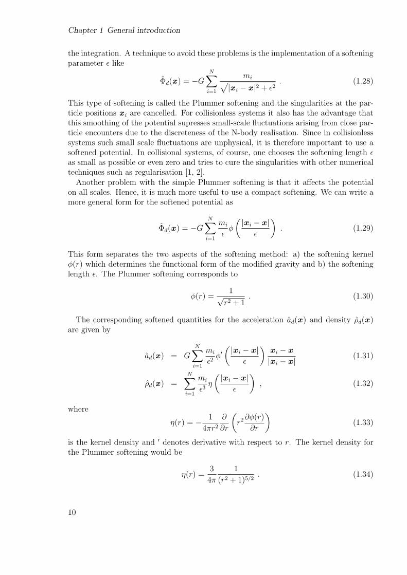
There are many possible choices for the functional form of the softening kernel φ(r).If the kernel density has compact support, then the gravity is not modified on distanceslarger than r0 from the particle, i.e. η(r) = 0 for r ≥ r0 and the accelerations areperfectly Newtonian for distances larger than r0 from the particle. Kernel densities thathave negative values near their outer edge correct for the underestimation of the acceler-ation near the origin and are therefore called compensating kernels. Hence, compact andcompensating kernels are the best choice one can make in order to soften the potentialand accelerations.
Following Dehnen [30], figure 1.2 shows different compact and compensating kernelsK0 −K3 compared with the Plummer scheme and the true Newtonian case. The func-tional form of the kernel Kn is given by
Kn =(2n + 5)!
(n + 1)! (n + 2)! 22n+6 π
(5− (2n + 7)r2
)(1− r2)n Θ(1− r2) (1.35)
where Θ is the Heaviside step function. Plotted are the potential (top panel), acceleration(middle panel; called force in the figure since here force denotes the force per mass) andthe density (bottom panel). The functions were scaled so that the maximum forceequals unity. The figure nicely illustrates the negative densities near the outer edgeof the kernels. The compact kernels join smoothly the Newtonian curves at the edgewhereas the Plummer scheme also modifies the gravity on larger scales. For a detaileddiscussion about the optimal softening scheme see also Dehnen [30] from which figure1.2 originates.
Direct method
A straightforward method to calculate the acceleration at position x would be the directsummation over all N particles in the N-body realisation
ad(x ) = G
N∑i=1
mix i − x
|x i − x |3 . (1.36)
In order to calculate the accelerations on all the N particles one needs exactly
N−1∑i=1
i =1
2N(N − 1) (1.37)
times to evaluate an acceleration. Hence, this method is of order O(N2) and the numberof particles one can use to represent the astrophysical system is limited by the immensecosts in evaluating forces in this approach. Normally only collisional systems that alsohave a small number of particles like globular clusters or star clusters are simulatedwith this technique. By designing special hardware that allows the calculation of theacceleration directly on the computer chip, the direct approach can be made practicalfor moderately large N (O(N) ≈ 106 − 107). This computer chip architecture is calledGRAPE which stands for GRAvity piPE and the operations needed for the calculationof the acceleration are directly hard-wired on the chip [96].
11

Chapter 1 General introduction
Figure 1.2: Different compact and compensating kernels K0−K3 are plotted and com-pared with the Plummer scheme and the true Newtonian case. Plotted arethe potential (top panel), acceleration (middle panel; called force in thefigure since here force denotes the force per mass) and the density (bottompanel). For further details see main text. Figure taken from Dehnen [30].
12

1.3 Numerical methods
Figure 1.3: Geometrical configuration for multipole expansion.
Hierarchical methods
By expanding the discrete gravitational potential around a point c and only accountingthe contribution to the potential of particles in a volume V around the point c, we canwrite a multipole expansion in cartesian coordinates
Φd(x ) = −G∑i∈V
mi
|x − c|∞∑
n=0
( |x i − c||x − c|
)n
Pn(cos(κi)) (1.38)
where Pn(cos(κi)) are Legendre polynomials. We have assumed that |x i − c| < |x − c|and the angles κi are defined by
cos(κi) =(x i − c) · (x − c)
|x i − c||x − c| . (1.39)
Figure 1.3 shows the geometrical configuration.
For n = 0 we have P0(cos(κi)) = 1 and the leading term in this series is given by
Φ0d(x ) = −G
1
|x − c|∑i∈V
mi
︸ ︷︷ ︸m0
d
, (1.40)
where m0d is called the monopole moment (or simply the total mass in the volume V ).
13

Chapter 1 General introduction
For n = 1 we have P1(cos(κi)) = cos(κi) and this term is given by
Φ1d(x ) = −G
∑i∈V
mi
|x − c||x i − c||x − c| cos(κi)
= −G(x − c)
|x − c|3∑i∈V
mi(x i − c)
︸ ︷︷ ︸m1
d
(1.41)
where m1d is called the dipole moment. We see that the higher order terms decay
rapidly with respect to the dominant monopole term. Higher order multipoles are calledquadrupole (n = 2), octupole (n = 3), hexadecapole (n = 4) etc.
By dividing up the space in different regions, we can approximate the contributionfrom a distant region V around c to the potential at a point x by using a multipoleexpansion and use only the leading terms in the expansion (1.38). By the superpositionprinciple, we can calculate the total potential at point x by summing up over all regions.The error by truncating the multipole expansion at some order can be controlled by thefollowing criterion
maxi∈V
(|x i − c|) < |x − c|θ (1.42)
where θ is called the opening angle. The geometrical interpretation is that the size ofthe region V (which we can measure by selecting maxi∈V (|x i− c|)) is not allowed to belarger than the distance |x − c| to that region times the opening angle θ; on the skyat position x , the region is not allowed to appear larger than the size controlled by theopening angle θ.
A common method to divide up the simulation space into different regions is to createa tree-structure by recursively subdividing the whole simulation space into smaller andsmaller subregions called cells. The standard method developed by Barnes and Hut [8]starts with a cubic cell with side length L that contains the whole simulation space.This cell is called the root cell. If a cell contains more than one particle it is subdividedinto eight sub-cells of side length L/2. This procedure is applied recursively until eachcell only contains one particle. This tree-structure is therefore called an oct-tree. Now,the simulation space is partitioned into cells of different sizes each containing only oneparticle and these cells are the leaves of the tree (sometimes also called buckets). Theaverage size of a leaf cell that contains only one particle is of the order of the interparticledistance h ∝ N−1/3 and and the typical number of subdivisions required to reach sucha leaf cell from the root cell (that is the height of the tree) is of order O(log2 N−1/3) =O(log N) and the time needed to construct the tree is of order O(N log N).
If one wants to calculate the acceleration of a particle at position x in the simulationthe following tree-walk procedure is applied. If a cell satisfies the condition (1.42) wherec is the centre-of-mass of the cell under consideration, the interaction via multipoleexpansion with this cell is accepted. If the cell fails the above criterion (1.42), thenits eight sub-cells are checked if they fulfill equation (1.42). This procedure is repeatedrecursively with all sub-cells. So, by starting at the root cell of the tree which contains the
14

1.3 Numerical methods
Figure 1.4: Quad-tree: the two dimensional version of the oct-tree in three dimensions.Each leaf cell contains only one particle. Left: the spatial configuration ofthe splittings. Right: Data structure represented as tree. Figure takenfrom Demmel [32].
whole simulation space one walks down the tree until one accepts a refined enough cell forthe interaction with the particle at x . If a leaf cell fails to fulfill the opening criterion,then its contribution to the acceleration is calculated directly as described in section1.3.4. As a result, the acceleration for a particle consists of a far-field part calculated fromthe multipoles and a near-field part calculated directly by particle-particle interactions.By following this procedure, the number of interactions for calculating the accelerationfor a particle is of order O(log N) for large N and the total cost scales like O(N log N).
Figure 1.4 shows the two dimensional version of the oct-tree. Each leaf cell containsonly one particle. The left panel shows the partitioning of space down to the leaves ofthe tree. On the right, the tree data structure is shown.
There exist many possible tree-structures like e.g. k-D tree [11] or binary tree [144]which mainly differ in the partitioning procedure. With tree-codes it is nowadays possibleto simulate of the order O(1010) particles as was done in the Millennium SimulationProject that simulated the evolution of the matter distribution in a cubic region of theuniverse of two billion light-years on a side from redshift z = 127 to the present [99, 143].
1.3.5 PKDGRAV
Throughout this thesis the state-of-the-art gravity code PKDGRAV was used. PKD-GRAV stands for Parallel K-D tree GRAVity code and was developed by Joachim Stadel
15

Chapter 1 General introduction
[144] and Thomas Quinn. The code uses a binary tree5 for the partitioning of space anda fourth order multipole expansion (i.e. terms up to the hexadecapole (n ≤ 4) in ex-pansion (1.38) are included) in order to calculate the accelerations from distant massin the simulations. Nearby contributions from leaf cells that fail to fulfill the openingcriterion are calculated directly. Potentials and accelerations are softened for distancessmaller than two softening lengths from a particle with the compact and compensatingsoftening kernel K1 described in section 1.3.4. The code is fully parallelised and thetime integration is done by a symplectic second order kick-drift-kick leapfrog scheme asdescribed in section 1.3.2.
1.4 Unifying both regimes
It is becoming apparent that many problems involve both high accuracy orbit calcula-tions to follow collisional scattering events and the need to simulate many particles inthe collisionless mean field limit.
For example, observations show that many galaxies contain a super-massive black holein their centre with masses correlated to the total bulge mass or dark matter halo mass[47, 58]. The nearest known super-massive black hole is located at the centre of ourown galaxy, the Milky Way. Figure 1.5 shows astrometric positions and orbital fits forseven stars around the central super-massive black hole in the centre of the Milky Way.The proper-motion measurements have uncertainties that are comparable to or smallerthan the size of the points, and are plotted in the reference frame in which the centralsuper-massive black hole is at rest. On the plane of the sky, three of these stars showorbital motion in the clockwise direction (S0-1, S0-2, and S0-16), and four of these starshave counterclockwise motion (S0-4, S0-5, S0-19, and S0-20). Overlaid are the best-fitting simultaneous orbital solutions, which assume that all the stars are orbiting thesame central point mass. Most of these stars are on orbits with very high eccentricitye → 1. The dynamics of these stars constrain the mass of the super-massive black holeto 3.7(±0.2)× 106 M¯ [42, 59, 60, 135].
Super-massive black holes are fascinating objects in our universe that can be used totest general relativity and structure formation in the universe [159]. They can also playan important role in influencing the local environment through dynamical processes aswell as regulating galaxy formation through feedback processes [101, 102, 103, 104, 106,138, 172]. Super-massive black holes also provide a natural explanation for the energyoutput of quasars, but how these black holes grow in a relatively short time scale in orderto explain the quasar activity at high redshift (4 < z < 6) is still unclear [73, 160, 162].At high redshifts it is thought that galaxy formation proceeds through a succession ofmerger events. If the proto-galaxies host black holes at their centres then they may alsomerge hierarchically to form a super-massive black hole. Gas accretion onto the centralobject may also play an important role in accelerating its growth [160, 161].
5PKDGRAV originally used a balanced k-D tree. However, for gravity calculations the balanced k-Dtree can behave pathologically in certain cases and it was replaced by a spatial binary tree structure[144].
16

1.4 Unifying both regimes
Figure 1.5: Astrometric positions and orbital fits for seven stars around the centralsuper-massive black hole in the centre of our own galaxy, the Milky Way.For further details see main text. Figure taken from Ghez et al. [60].
17

Chapter 1 General introduction
Hence, understanding the combined formation, dynamics and evolution of these blackholes, the dark matter haloes and the stellar systems that they are embedded within,requires a unification of the two N-body regimes discussed above.
This means the interaction between collisionless particles like dark matter and starsis still treated in the mean field limit and the short range forces are softened in ordernot to suffer from artificial gravitational scattering. In regions where the potential isdominated by e.g. a super-massive black hole, it is important to follow the 2-body orbitsaround the black holes correctly.
We can define the gravitational influence radius of a single super-massive black holeas the distance within which the potential is dominated by the super-massive blackhole, rather than by the smooth background potential created by all the other particles[102, 103]. A standard definition for the radius of influence rinfl of a single super-massiveblack hole is the solution to
r =GMSMBH
σ2(r), (1.43)
where σ(r) is the one dimensional velocity dispersion of the surrounding system andMSMBH is the mass of the super-massive black hole. This equation can often only besolved numerically. Hence, an alternative definition of the radius of influence is frequentlyused where rinfl is given by the radius that encloses two times the super-massive blackhole mass,
M(rinfl) = 2MSMBH , (1.44)
where M(r) is the cumulative mass of the surrounding system assuming spherical sym-metry. If the density profile of the surrounding structure is that of a singular isothermalsphere given by [15]
ρ(r) =σ2
2πGr2, (1.45)
where the velocity dispersion is constant and independent of radius, the two definitionsin equations (1.43) and (1.44) are equivalent. If we calculate the radius of influence forthe dark matter in a Milky Way size halo we get of the order of a few dozen pc6 and forthe central stellar bulge in the Milky Way a few pc.
This is a very difficult dynamical problem with spatial scales ranging from pc to Mpc(as a typical separation of two galaxies) and time-scales ranging from a few yr for anorbit around the super-massive black hole to a few Gyr which is the time-scale neededfor the merger of the two galaxies.
1.5 Content of this thesis
The main goal of this doctorate thesis was the development of the N-body tools thatcan follow the evolution of dark matter haloes on Mpc scales, which host central super-massive black holes that can modify structure and dynamics on pc scales. This problem
6pc stands for parsec and is a widely used length unit in astrophysics. 1 pc = 3.086× 10¹⁶ m.
18

1.5 Content of this thesis
not only includes a wide spatial range of six orders of magnitudes but also a hugetemporal range of approximately nine orders of magnitude.
Chapter 2
In order to resolve pc scales in a dark matter halo, of order O(1010) particles would beneeded. This is clearly not feasible with today’s supercomputers and one has to makecertain approximations. Here, we present a newly developed multi-mass technique forbuilding dark matter haloes for N-body simulations. With this technique we only resolvethe very central part of a dark matter structure with the effectively needed resolutionand use lower resolution in low density regions of the simulations, i.e. the outskirts ofthe haloes. This technique pushes the resolution scale to much smaller scales for givencomputational costs.
Chapter 3
In order to follow the dynamics correctly, the development of a physically motivatedtime-stepping scheme was needed. Previous time-stepping schemes based on the accel-eration of the particles and which are commonly used in N-body simulations were notable to follow the very active dynamics in the centres of galaxies and in certain caseseven delivered unphysical time-steps. Additionally, the acceleration based scheme is notsuitable for high resolution simulations since it has a bad scaling with the number ofparticles used in the N-body realisation. We developed a scheme based on the truedynamical time of a particle and implemented this within the tree-code PKDGRAV.This scheme always sets a physically motivated time-step for a particle in the N-bodysimulation. It also shows the optimal scaling with the number of particles used in theN-body simulations. The detailed ideas and implementation scheme is presented in thischapter.
Chapter 4
Here, we present applications of the new developments that were already carried out sofar. In the first application, the the multi-mass technique was used in a cosmologicalstructure formation run in order to resolve the resulting density profile of a high res-olution cluster down to one per mill of the virial radius. This resolution correspondsto one billion particles within the virial radius and is the N-body simulation with thehighest resolution so far performed. The second application used multi-mass modelsin order to test a potential explanation of the presence of the five globular clusters atapproximately 1 kpc distance form the centre of the Fornax dwarf spheroidal galaxy. Forthis purpose, cuspy and cored dark matter haloes with an effective resolution of orderof O(108) particles were used.
19

Chapter 1 General introduction
Chapter 5
A summary and a perspective on future projects and applications are then presented inchapter 5.
20
Chapter 2
Multi-mass halo models
2.1 Introduction and motivation
Resolution is a key issue in N-body simulations. In state-of-the-art N-body simulationstoday, structures can be fully resolved down to the scale of a fraction of a per cent of thevirial radius. But there are many problems, where higher resolution in central regionsof structures is needed.
For example, the question if the central dark matter density profile of haloes thatform in cosmological N-body simulations is cuspy or cored needs at least a resolutionof approximately 10−3 rvir to be answered. Another example are flat/cored central haloprofiles: in order to resolve structures with cored central profiles, a lot of particles areneeded since in flat profiles the resolution scaling with the number of particles is theslowest (see below for more details about the scaling of resolution with the number ofparticles). One further problem that was especially in mind when developing the multi-mass technique, was the dynamics of super-massive black hole binaries in the centreof remnants of galaxy mergers. There, the relevant scales are of order of a few pc≈ 10−6 − 10−5 rvir for Milky Way size dark matter haloes.
We illustrate the resolution problem in more detail with a commonly used family ofspherically symmetric density profiles used for haloes in N-body simulations: the socalled αβγ-models family [29, 71, 176]. An αβγ-model density profile is given by
ρ(r) =ρ0
(rrs
)γ (1 +
(rrs
)α)(β−γα )
, r ≤ rvir , (2.1)
where γ determines the inner and β the outer slope of the density profile whereas αcontrols the transition between the inner and outer region. The normalisation is givenby ρ0 and rs is the scale radius defined by rs ≡ rvir/c (c is called concentration). Thetwo most famous models that belong to this family are the Moore [110] profile with(α, β, γ) = (1.5, 3.0, 1.5) and NFW [116] profile with (α, β, γ) = (1.0, 3.0, 1.0).
The resolution scale mainly depends on the number of particles Nvir that samples thestructure chosen by the simulator. We can define the mean particle separation as afunction of radius in such a structure by
h(r) ≡ 3
√m
ρ(r), (2.2)
21

Chapter 2 Multi-mass halo models
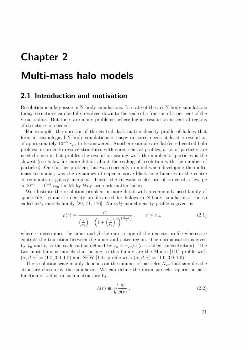
Figure 2.1: Mean particle separation function for a dark matter halo with central slopeγ = 1.0 (left) respectivley γ = 1.5 (right). We used values of Nvir =(106, 108, 1010) = (solid, dotted, dashed) to evaluate the function. Thecrossing with the diagonal line corresponds to h(r) = r, i.e. the crossingradius is rimp.
where m is the mass per particle. For single-mass models, the mass per particle is simplygiven by m = Mvir/Nvir and we get for the asymptotic scaling in the central part of thestructure h(r) ∝ rγ/3.
In figure 2.1 we plot the mean particle separation for a dark matter halo with centralslope γ = 1.0 (left) respectivley γ = 1.5 (right) with Mvir = 1012 M¯/h = 1.429 ×10¹² M¯ (h = 0.7)1. The concentrations were chosen so that the radius where themaximum circular velocity is reached are equal, i.e. c1.0 = 10 and c1.5 = 5.779 [173].We used the following values for the number of particles within the virial volume Nvir =(106, 108, 1010) = (solid, dotted, dashed) to evaluate the function given by equation (2.2).The innermost particle in a model sampled with Nvir particles is approximately locatedwhere we have h(r) = r (r is the distance from the geometrical centre). This sets thesmallest scale in the physical problem and we call this radius rimp, i.e. h(rimp) = rimp.But of course one particle is not enough to resolve that scale. If we say we need at leastof the order of ≈ 100 particles in the innermost bin so that the bin is well resolved, theneach h(r) function gets a shift of factor 3
√100 ≈ 4.6 upwards in figure 2.12. Generally,
the scaling of rimp is given by
rimp ∝ 3−γ√
m ∝ 3−γ
√1
Nvir
. (2.3)
1h denotes the Hubble constant H in units of 100 km s−1 Mpc−1. H = 100 h km s−1 Mpc−1
2Apart from a geometrical factor that is of the order of unity for the two profiles with γ = 1.0respectively γ = 1.5, this corresponds to the radius that includes 100 times the mass of one particle.
22

2.2 Method
in the region where the slope of the profile is close to −γ in the αβγ-profiles (theinner region). Equation (2.3) illustrates the resolution gain by increasing the number ofparticles Nvir and its dependence on the central density profile slope γ.
By inspecting figure 2.1, we see that we need more than approximately of order O(1010)particles in the centre in order to resolve scales of 10−6 − 10−5 rvir which correspond toapproximately 1 pc in physical units in this model. It is worth remarking, that with thesame number of particles Nvir much smaller scales are resolved in the steeper profile withγ = 1.5 than in the γ = 1.0 profile although the concentration was lower. Generally,the steeper the central profile, the more the particles are concentrated. Nonetheless,this enormous amount of particles per dark matter halo is hardly doable today - evenwith large supercomputers like zBox23, a large 125 nodes cluster with in total 500 64bit cpus on quad-boards. But since we only need this high resolution at the very centreof the dark matter halo, our solution to this problem is the usage of haloes with shellsof different resolution, i.e. we use light particles with a small mean particle separationin the centre and heavy particles in the outer parts of the halo.
2.2 Method
The technique for generating multi-mass equilibrium haloes is based on the methodpresented in Kazantzidis et al. [80]. We give here a short review of the procedure.
We can choose the density profile from the αβγ-models family given by equation (2.1)for r ≤ rvir with concentration c, profile slopes α, β and γ, virial mass Mvir, and numberof particles Nvir as input parameters. This determines the normalisation ρ0 and thescale radius rs for a chosen cosmology. Beyond the virial radius, an exponential cut-offis applied. For further details see Kazantzidis et al. [80] and Zemp [173]. The particlepositions are initialised from the cumulative mass function M(r). With the particle’spositions, the acceptance-rejection technique [87] is used to determine its velocity fromthe distribution function and the velocity structure is chosen to be isotropic. Thisprocedure leads to perfectly stable equilibrium models as was shown in Kazantzidiset al. [80]. These models do not show the flattening in the central part of the haloduring evolution as it is obtained in the case of the assumption of a local Maxwellianvelocity distribution.
In the multi-mass case, one has the choice to introduce different spherical shells withdifferent particle masses, i.e. the central shell is populated by light particles and theouter shell is populated by heavy particles. Initially, the different species are strictlyseparated but with time the different species mix and form stable sub-profiles whileleaving the total mass profile unchanged.
Of course this technique introduces some further numerical artefacts as e.g. heatingof the light particles by the heavy particles or mass segregation of the heavy outerparticles. The dynamical friction force that a particle of mass M experiences in a sea of
3www.zbox2.org
23
Chapter 2 Multi-mass halo models
light particles with mass m ¿ M is [15, 21]
Fdf ∝ M2 (2.4)
and the time-scale for this particle to reach the centre of the structure is
Tdf ∝ M−1 . (2.5)
Hence, by choosing moderate mass ratios we can reduce the effect of mass segregation.By scaling the softening lengths of the heavy particles as a function of their mass, alsoartificial 2-body scattering can be reduced. For further details about the scaling of thesoftening, see section 2.3.
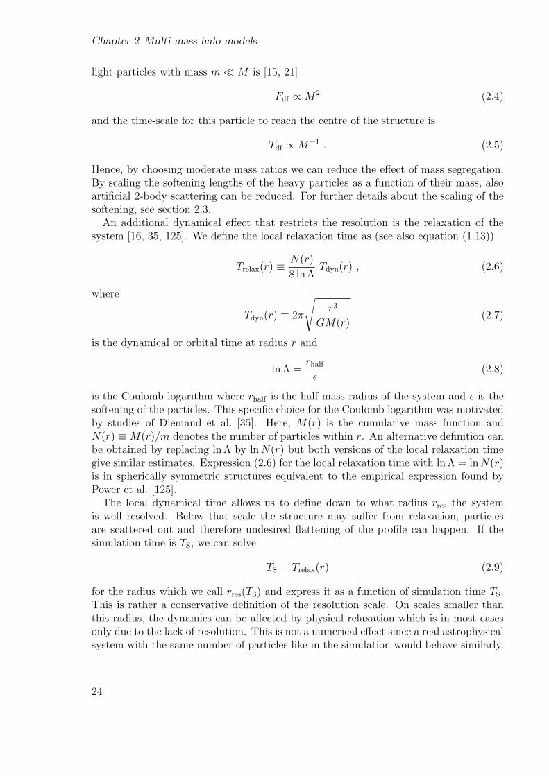
An additional dynamical effect that restricts the resolution is the relaxation of thesystem [16, 35, 125]. We define the local relaxation time as (see also equation (1.13))
Trelax(r) ≡ N(r)
8 ln ΛTdyn(r) , (2.6)
where
Tdyn(r) ≡ 2π
√r3
GM(r)(2.7)
is the dynamical or orbital time at radius r and
ln Λ =rhalf
ε(2.8)
is the Coulomb logarithm where rhalf is the half mass radius of the system and ε is thesoftening of the particles. This specific choice for the Coulomb logarithm was motivatedby studies of Diemand et al. [35]. Here, M(r) is the cumulative mass function andN(r) ≡ M(r)/m denotes the number of particles within r. An alternative definition canbe obtained by replacing ln Λ by ln N(r) but both versions of the local relaxation timegive similar estimates. Expression (2.6) for the local relaxation time with ln Λ = ln N(r)is in spherically symmetric structures equivalent to the empirical expression found byPower et al. [125].
The local dynamical time allows us to define down to what radius rres the systemis well resolved. Below that scale the structure may suffer from relaxation, particlesare scattered out and therefore undesired flattening of the profile can happen. If thesimulation time is TS, we can solve
TS = Trelax(r) (2.9)
for the radius which we call rres(TS) and express it as a function of simulation time TS.This is rather a conservative definition of the resolution scale. On scales smaller thanthis radius, the dynamics can be affected by physical relaxation which is in most casesonly due to the lack of resolution. This is not a numerical effect since a real astrophysicalsystem with the same number of particles like in the simulation would behave similarly.
24

2.3 Tests
The problem is that in the near future we can not simulate of the order of O(1070) darkmatter particles like the real astrophysical system would have. Therefore, this effect dueto under-resolving the system with not enough particles will always be a limitation toN-body simulations.
In principle, the only known dynamically stable system in the universe is the Keplerian2-body system.4 Dynamical effects like relaxation or evaporation will sooner or later leadto the disruption of any system. It is therefore always a question within what time-scalethe system is stable. The time-scale of interest is normally of order of the age of theuniverse and for most cases the astrophysical systems can be regarded as perfectly stablewithin that time-scale. This is different in N-body simulations. Here, one just triesto generate models that show the desired stability behaviour during the time-scale ofinterest with the least amount of particles needed. It is therefore clear that the artificialN-body models show these disruption effects much sooner since they are not modeledwith the true number of particles like the real astrophysical system one wants to study.
In section 2.3, we show that by a careful choice of parameters like mass ratio betweenthe different species and softening length, these effects on global characteristics like theradial density profile are small. The multi-mass technique is therefore an efficient methodto perform high resolution N-body simulations.
2.3 Tests
2.3.1 Two-shell models
We performed a series of runs in order to show how the multi-mass model works andto illustrate the limits of this method. In this series we chose four different profilesfrom the αβγ-family described by equation (2.1). We chose for the different haloes avirial mass of Mvir = 1012 M¯/h = 1.429 × 10¹² M¯ (h = 0.7) which correspondsto a virial radius of rvir ≈ 289 kpc and a virial density ρvir = 1.408 × 10⁴ M¯ kpc−3
(spherical overdensity ≈ 100 ρcrit in a standard ΛCDM-cosmology [45]). The followingdensity profile parameters were the same for all models: outer profile β = 3, transitioncoefficient α = 1 and concentration c = rvir/rs = 20 (rs is the scale radius). We variedthe inner profile form γ = 0.0 . . . 1.5 and chose for the shell radius the scale radius, i.e.rshell = rs. We resolved the density profile within rshell always with 300000 particles andchanged the number of particles in the outer shell for the other runs so that the massratio had the following values 1× 100, 3× 100, 1× 101, 3× 101, 1× 10², 3× 10², 1× 10³.The choice of softening for the light particles εlight and the total number of particles Nvir
in the case of equal mass particles in the inner and outer shell as well as the estimatedresolution scale after 10 Gyr, rres(10 Gyr), are given in table 2.1. The softening lengthsof the heavy particles were scaled like rimp (equation 2.3), i.e.
εheavy = εlight3−γ
√mheavy
mlight
= εlight3−γ√
RM (2.10)
4This is only true in the Newtonian regime. In General Relativity, not even a 2-body orbit is dynam-ically stable and the orbit decays due to the emission of gravitational radiation [5, 41, 74].
25
Chapter 2 Multi-mass halo models
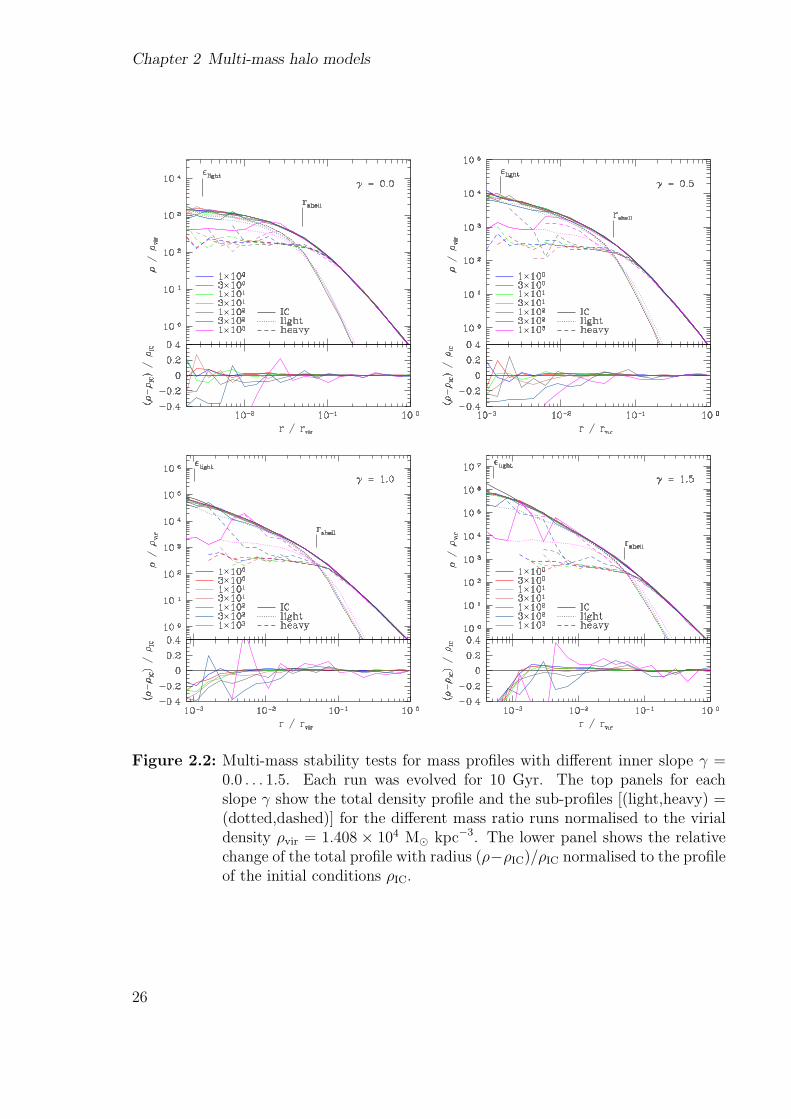
Figure 2.2: Multi-mass stability tests for mass profiles with different inner slope γ =0.0 . . . 1.5. Each run was evolved for 10 Gyr. The top panels for eachslope γ show the total density profile and the sub-profiles [(light,heavy) =(dotted,dashed)] for the different mass ratio runs normalised to the virialdensity ρvir = 1.408 × 10⁴ M¯ kpc−3. The lower panel shows the relativechange of the total profile with radius (ρ−ρIC)/ρIC normalised to the profileof the initial conditions ρIC.
26

2.3 Tests
γ 0.0 0.5 1.0 1.5εlight 0.9 kpc 0.45 kpc 0.3 kpc 0.15 kpc
≈ 3.1× 10⁻³ rvir ≈ 1.6× 10⁻³ rvir ≈ 1.0× 10⁻³ rvir ≈ 5.2× 10⁻⁴ rvir
Nvir 7.215× 10⁶ 4.880× 10⁶ 3.250× 10⁶ 2.112× 10⁶
rres(10 Gyr) ≈ 1.42 kpc ≈ 1.35 kpc ≈ 1.25 kpc ≈ 1.15 kpc≈ 4.9× 10⁻³ rvir ≈ 4.7× 10⁻³ rvir ≈ 4.3× 10⁻³ rvir ≈ 4.0× 10⁻³ rvir
Table 2.1: Summary of parameters for the different models. The rows are softening ofthe light particles, εlight, total number of particles in the equal mass case,Nvir, and estimated resolution radius after 10 Gyr, rres(10 Gyr).
where RM is the mass ratio of the heavy to the light particles. Each of these 28 modelswas evolved in isolation for 10 Gyr in order to test the stability of the structures withPKDGRAV (see section 1.3.5). In order to follow the dynamics in the centre correctly,we used the dynamical time-stepping scheme developed by Zemp et al. [174] (see chapter3).
In figure 2.2, we present the density profiles of these runs after 10 Gyr. For moderatemass ratios RM up to 10-30 (or even RM ≈ 100 for steep central profiles) the effects onthe total density profile are small and the profile remains stable down to the level of a fewεlight. Such deviations are anyway expected since the forces in PKDGRAV are softenedif two particles have separations of order of their softening length. By comparing theequal mass cases for the two steepest central profiles, we see that the flattening effectdue to relaxation sets in at a factor 2-3 times smaller radius than the estimated valuerres(10 Gyr), confirming that it is rather a conservative estimate.
The same behaviour is also seen in the anisotropy profiles. In figure 2.3, we plot thevelocity anisotropy parameter defined by
β(r) ≡ 1
2
σtan(r)
σrad(r), (2.11)
where σtan(r) is the tangential velocity dispersion and σrad(r) is the radial velocity dis-persion in a spherical coordinate system as a function of radius r. For isotropic systemswe obtain β(r) = 1.5 We see again that for moderate mass ratios up to approximately30 the velocity anisotropy profile stays isotropic.
Figure 2.2 also illustrates that the different species form stable sub-profiles. The shellradius was chosen in a zone where the local density profile is steep so that the transitionregion is small and in the inner or outer region the light respectively heavy particlesdominate. Only for very high mass ratios, the total density profile is strongly perturbedby heating effects of the heavy particles and the heavy particles sink to the centre dueto the better efficiency of dynamical friction. But for moderate mass ratios, these effectsare small and expected only for much longer time-scales.
5This definition deviates from the standard definition normally used e.g. in Binney and Tremaine [15].Normally, βstd = 1 − β but since we plot the relative change with respect to the isotropic initialconditions (which would be βstd = 0) we used this alternative definition.
27

Chapter 2 Multi-mass halo models
Figure 2.3: Multi-mass stability tests for mass profiles with different inner slope γ =0.0 . . . 1.5. Each run was evolved for 10 Gyr. The top panels for each slopeγ show the anisotropy profile for the different mass ratio runs. The lowerpanel shows the relative change of the total profile with radius (β−βIC)/βIC
normalised to the profile of the initial conditions βIC.
28

2.3 Tests
Figure 2.4: The computer run time T needed for the 10 Gyr stability run described inthe text is plotted as a function of mass ratio RM for the different centralprofiles γ. T0 is the computer run time needed for the equal mass run. Asubstantial fraction of time is gained in all cases. Most of the time gain isalready obtained for small mass ratios.
29
Chapter 2 Multi-mass halo models
The main advantage of these multi-mass models is the speed up gain. In figure 2.4,we plot the computer run time T needed for the 10 Gyr stability test run describedabove as a function of mass ratio RM. We normalise with the time T0 needed by theequal mass run. Figure 2.4 illustrates that we gain a substantial fraction of computerrun time in all cases. Most of the gain is already obtained for small mass ratios RM.For example, the run with inner slope γ = 0.0 and mass ratio RM = 10 is approximatelyfour times faster that the same run without multi-mass refinement and does not showany perturbation effect of the multi-mass technique on the density profile. Therefore,the usage of too high mass ratios is not recommended since most of the computationalwork in the simulation comes form the central part and too high mass ratios only leadto larger perturbations of the models.
The steeper the central profile, the less is the computer run time gain. This is due tothe fact that most of the work in the N-body simulation for steep profiles is concentratedin the centre. In the centre, the particles are on very small time-steps compared tothe less dense, outer regions of a dark matter halo in an N-body simulation and as aconsequence a lot of expensive force calculations are needed. It is especially dramatic ifone does the dynamics correct by using a dynamical time-stepping criterion rather thanthe ad-hoc criterion based on the acceleration which can even lead to completely wrongand unphysical time-steps in high resolution N-body simulations. See also chapter 3 formore details about this. That is simply the price one has to pay for correct physics!Using a hierarchy of trees where one freezes part of the simulation during the N-body runcould be a promising solution in order to perform high resolution N-body simulations inthe future and is under development.
2.3.2 Three-shell models
This method also works for three shells with different mass resolutions. In figure 2.5,we present a profile with central slope γ = 1.0 that has the same general specificationslike virial mass, virial radius, virial density, concentration as the models described insection 2.3. The shell radii were set at rshell,1 = 2 kpc respectively rshell,2 = 10 kpc. Weput in each shell 3 × 10⁶ particles resulting in mass ratios of mmedium/mlight ≈ 13.53mheavy/mlight ≈ 245.9 and mheavy/mmedium ≈ 18.17. This configuration corresponds toan effective resolution in the centre of N eff
vir = 7.8 × 10⁸ particles. The softening of thelightest species was εlight = 0.05 kpc ≈ 1.7× 10⁻⁴ rvir. The softening length of the otherparticles was scaled according to relation (2.10).
Fiugre 2.5 illustrates that the total profile of the three-shell model is stable over 10Gyr down to approximately 3×10⁻⁴ rvir. The total profile fluctuates only a few per centover 3.5 orders of magnitude in space. This was only possible by using the multi-masstechnique where we used in total approximately only 107 particles in order to generatea model that has an effective central resolution of N eff
vir = 7.8× 10⁸ particles.
30

2.3 Tests
Figure 2.5: The total profile of the three-shell model is stable over 10 Gyr down toapproximately 3× 10⁻⁴ rvir. Fluctuations in the total profile are on a fewper cent level.
31

Chapter 2 Multi-mass halo models
γ 0.0 1.0εlight 0.48 kpc 0.3 kpc
≈ 1.7× 10⁻³ rvir ≈ 1.0× 10⁻³ rvir
N effvir 4.812× 10⁷ 5.232× 10⁷
rres(10 Gyr) ≈ 0.77 kpc ≈ 0.40 kpc≈ 2.6× 10⁻³ rvir ≈ 1.4× 10⁻³ rvir
Table 2.2: Summary of parameters for the two initial conditions used for the merg-ers. The rows are softening of the light particles, εlight, effective number ofparticles in the haloes, N eff
vir, and estimated resolution radius after 10 Gyr,rres(10 Gyr).
2.4 Preservation of cusp slope
Dehnen [31] showed that in a merger of self-gravitating cusps with different central slopesthe merger remnant has always the slope of the steepest progenitor. In other words thesteepest cusp slope should be preserved.
Collisionless mergers of dark matter haloes were already studied in earlier work [e.g.4, 16, 114] but none of these studies had the resolution of the simulations presented here.We do not find any discrepancies between this work and the earlier studies and see thistherefore more as a confirmation that the multi-mass technique works in the extremedynamics of a dark matter halo merger event.
We initially set-up two dark matter halo models with different central slope. Bothprofiles were from the αβγ-model family (see equation (2.1)) and had a virial mass ofMvir = 1012 M¯/h = 1.429 × 10¹² M¯ (h = 0.7) which corresponds to a virial radius ofrvir ≈ 289 kpc, a virial density ρvir = 1.408×10⁴ M¯ kpc−3 and a concentration of c = 20.That are the same general specifications as the models described in section 2.3. Theouter slope was fixed to β = 3, the transition coefficient was set to α = 1 in both cases.One profile had an inner slope of γ = 0.0 and a shell radius of rshell = rs = 14.47 kpc.The other profile had a central slope of γ = 1.0 and a shell radius of rshell = 5 kpc. Inboth cases, a mass ratio of RM = 20 between heavy and light particles was chosen. Forsoftening and effective number of particles see also Table 2.2. The softening lengths ofthe heavy particles were scaled according to relation (see also equation 2.10)
εheavy = εlight3−γ
√mheavy
mlight
= εlight3−γ√
RM . (2.12)
The resolution is clearly limited by the centrally flat (γ = 0.0) model since here muchmore particles are needed to resolve a given scale compared to steeper profiles. To resolvethe same scale with the steep profile much less particles would be needed, but since wewould not like to have too high mass ratios between any species of particles involved inthe merger we adjusted the number of particles in the profile with γ = 1.0 so that itsparticles had similar masses as the particles in the γ = 0.0 model.
We evolved both haloes in isolation for 10 Gyr in order to test the stability again. Intotal three mergers were performed: a cusp-cusp, a core-core and a cusp-core merger
32

2.4 Preservation of cusp slope
Figure 2.6: Equal profile mergers, left: γ = 0.0 and right: γ = 1.0. The profiles arestable over 10 Gyr and the central profile is conserved in both cases.
where cusp means γ = 1.0 and core is equivalent to the γ = 0.0 model described above.The following merger set-up was used. We placed the two haloes 600 kpc ≈ 2 rvir apartand the the two haloes had an initial relative radial velocity of vrad ≈ 150 km s−1 anda relative tangential velocity of vtan ≈ 50 km s−1. Assuming the two haloes were pointmasses, this set-up correspond to an eccentricity e ≈ 0.95 of the orbit consistent withvalues in cosmological N-body simulations [81]. With this set-up the merger time neededby the two haloes to merge completely was approximately 7 Gyr. We let all three runsevolve to 10 Gyr so that the merger remnant had time to relax.
Figure 2.6 shows the stability of both models and the equal profile mergers after 10Gyr. Down to a few softening length of the light particles no significant deviations canbe seen in the stability tests. The merger remnant has the same profile as the twoprogenitors except that the local density more or less doubles. We normalise the plotsby the values rvir and ρvir of the progenitor haloes. The deviations in the outer part ofthe profiles are due to a slightly triaxial shape of the halo there. The remnant just didnot have enough time to fully relax in this region.
In figure 2.7, we present the profile of the cusp-core merger after 10 Gyr. The centralslope of the steepest progenitor is perfectly preserved and the cored progenitor onlycontributes significantly in the outer region of the total density profile.
We can therefore confirm the earlier findings that core-core mergers lead to a coredmerger remnant while cups-cusp mergers lead to a cuspy merger remnant with highresolution multi-mass N-body simulations. In cusp-core merges the merger remnant hasa final profile corresponding to the steepest progenitor which is in excellent agreementwith the prediction by Dehnen [31].
33

Chapter 2 Multi-mass halo models
Figure 2.7: Cusp-core merger after 10 Gyr. The central cusp is preserved. Plotted arealso the sub-profiles of each particle species in the simulation and the indi-vidual profiles of the two progenitors with central slope γ = 0.0 respectivelyγ = 1.0.
34

2.5 Conclusions
2.5 Conclusions
The multi-mass technique for modelling haloes is a simple method in order to performhigh-resolution N-body simulations. The following rules of thumb should lead to wellbehaving structures:
• The mass ratios between particles of neighbouring shells should not be too high.We recommend from RM ≈ 20− 30 for flat profiles up to maximum RM ≈ 100 forsteep profiles.
• The softening length should scale according to the mass of the particle, i.e. highmass particles should have bigger softening than low mass particles in order toprevent heavy scattering.
• The shell radii should be set at places where the local density profile is steep sothat the transition region where different species contribute equally is as small aspossible.
• The density profiles are only stable down to the radius rres which depends on thetime TS the simulator wants to simulate. Below that scale, relaxation will lead toflattening of the density profile. For a given computer run time TS, this implies aminimum effective number of particles.
The multi-mass technique can lead to a significant gain in computer run time for agiven resolution scale and is therefore ideally suited for many applications in N-bodysimulations.
35

Chapter 2 Multi-mass halo models
36

Chapter 3
An optimum time-stepping scheme forN-body simulations1
3.1 Introduction
Achieving spatial adaptivity in the evaluation of forces in N-body simulations is a wellstudied problem with many effective approaches based on the use of tree structures andmultipole expansions or nested grids and FFT techniques. Such adaptivity in space alsocomes with a desire to achieve adaptivity in the time integration of these simulationssince a large dynamic range in density implies a large dynamic range in time-scales forself gravitating systems (T ∼ 1/
√Gρ ). Two very different problems present themselves
when trying to achieve this. First, there are no practical (explicit), general purpose(applicable to a wide range of astrophysical problems), adaptive integration techniquesknown for the N-body problem which are symplectic. By this we mean that the numer-ical integration is an exact Hamiltonian phase flow very close to the phase flow of thecontinuous system under study. This is a very desirable property for following systemsfor longer than a single dynamical time. Such exact preservation of the geometricalproperties of the dynamical system is possible for fixed time-step schemes. For generalN-body simulations with adaptive time-stepping we have to resort to approximate sym-plectic behaviour or preservation of time symmetry (a property which is known to leadto very good integration methods). The second problem is that of continuously deter-mining the appropriate time-step for each particle in the simulation so that the errorin the integration remains within tolerance while performing the fewest possible forceevaluations and minimising the computational overhead. Resolving this second problemis the main focus of this chapter and can be considered independently from methodssymmetrizing the time-stepping scheme such as presented in in work by Stadel [144] andMakino et al. [97].
There are several known time-step criteria based on different properties of the sim-ulation (e.g. local density ρ(r), potential Φ(r), softening ε, acceleration a, jerk a oreven the velocity v of the particle) that are used in state-of-the-art numerical codes[1, 125, 128, 141, 144]. Some of them have a physical motivation, others are just aclever combination of physical properties in order to obtain a criterion which has thephysical unit of time. All are an attempt to find an inexpensive way of determining an
1This chapter is a slightly modified version of Zemp et al. [174].
37

Chapter 3 An optimum time-stepping scheme
appropriate time-step for each particle in the simulation. For cosmological simulations,the ad-hoc time-step criterion based on the acceleration and the gravitational soften-ing of the particle (T ∼
√ε/a ) has proven very successful, despite the fact that it is
not directly related to the dynamical time in these simulations. One reason why thistime-step criterion is thought to work well is that it results in a very tight time-stepdistribution with very infrequent changes in the time-step of a particle in block time-stepping schemes (power of 2 step sizes; see also section 3.2.2). This hides the evilsdue to the first problem since the behaviour is more like that of a fixed time-steppingscheme than for other criteria. The price however is that more time-steps are taken inlower density regions of the simulation than would seem to be necessary. Furthermore,while still adequate for the type of simulations that have been performed up to now,which adapt the softening and mass of particles in the highest density regions and thusreduce the time-step somewhat artificially in those regions, this time-stepping scheme isno longer effective in simulations covering a much larger dynamic range.
In state-of-the-art computer simulations, structures can be resolved by Nvir ≈ O(107)which results in a resolution scale of rres ≈ O(10−3 rvir). By comparing the dynamicalscales at rvir and rres, we get Tdyn(rvir)/Tdyn(rres) ≈ O(103) or even larger for future highresolution simulations. This large dynamical range in time-scales demands an acutelyadaptive criteria so that the dense, dynamical active regions are resolved correctly whilethe simulations remain fast.
However, in a general simulation, such as those used for cosmological structure forma-tion, it is not straightforward to determine the dynamical time of a given particle. Thisdepends on the dominant structure responsible for the orbit of a particle which needsto be quickly determined at each time-step as the particle is advanced. In this chapterwe develop a new fast method of determining each particle’s true dynamical time us-ing information directly computed in the force evaluation stage of the simulation. Thisis quite different from using the local dynamical time which fails dramatically undermany circumstances, e.g. consider using the local density near the earth to estimate itstime-step!
3.2 Dynamical time-stepping
3.2.1 General idea and description
In order to advance a particle in a numerical simulation, we have to choose a particulartime-step for each individual particle. Let us consider a particle on a circular orbit ina system with spherical symmetric density profile ρ(r). The dynamical time Tdyn(r) (ororbital time) of this particle at radius r under spherical symmetry is given by
Tdyn(r) ≡ 2π1√
Gρenc(r), (3.1)
where
ρenc(r) ≡ M(r)
r3(3.2)
38

3.2 Dynamical time-stepping
is the enclosed density within the radius r and M(r) is the total mass within radius r.The natural choice for a time-step of a particle would therefore be ∆T ∝ Tdyn were wenot faced with the difficulty of determining the enclosed density.
For a particle in a given landscape of cosmic structure, the enclosed density shouldbe set, roughly speaking, by the structure that the particle is orbiting about. Withincollisionless cosmological simulations this could be some super-cluster scale structure, oran individual dark matter halo, or some substructure within a dark matter halo. Ideally,we would scan the whole sky of the particle and determine the structure that gives thedominant contribution to its acceleration. From this dominating structure, we coulddetermine the enclosed density and hence find the dynamical time of the particle.
Here we have to distinguish two different regimes. First, we have the mean fieldregime, i.e. particles move in a (slowly) varying potential that is determined by thetotal mass distribution. The individual particles are only weakly influenced by theirdirect neighbours and their motions are dictated by the sum of more distant particles.This is ensured by appropriately softening the short range force thereby placing anupper limit on the contribution from an individual particle. In this regime we want theenclosed density to be set by the globally dominating structure. The second regime isthe gravitational scattering regime where we would like to follow large angle scatteringdue to gravitational interactions, i.e. orbits with eccentricity e → 1. Here it is importantto get the contributions from the closest neighbours which dictate the orbital evolutionwhen they are very close and when there is little or no force softening. This means thatthe enclosed density is often set by some locally dominating particle.
The determination of the enclosed density is quite easy for some simple configurationslike the 2-body problem or a particle orbiting an analytically given spherical symmetricstructure. However, the generalisation to any given configuration in an N-body simula-tion is not so straightforward and we present a simple way in which this can be achievedwithin a tree based gravity code. The specific implementation within other code-typesmay look somewhat different but the general scheme and spirit of the method stays thesame.
3.2.2 Implementation within a tree-code
We use the tree-code PKDGRAV written by Stadel [144, see also section 1.3.5] whichallows for an adaptive time-stepping mechanism where each particle can be on a differenttime-step. The time-steps of the particles are quantized in fractions of powers of twoof a basic time-step T0 (block time-stepping). Therefore, particles on rung n have anindividual time-step of
∆T =T0
2n, (3.3)
where T0 is the basic time-step of the simulation and can be chosen by the simulator.As stated previously, our time-stepping criterion is given by,
∆TD =T0
2n≤ ηD
1√Gρenc(r)
, (3.4)
39

Chapter 3 An optimum time-stepping scheme
where ηD is a free parameter. Therefore, we need to calculate the enclosed density ρenc
for each particle from information that is available in a tree-code in order to determineits rung.
In hierarchical tree-codes, at every time-step two interaction lists are generated foreach particle: a list of multipoles and a list of particles that interact with the givenparticle. The tree structure in such codes is a hierarchical representation of the mass inthe simulation with each subvolume, or cell, being a node in this tree. As we proceed fromthe root to the leaves of this data structure we get an ever finer mass representation ofthe simulation. The forces from more distant cells are calculated by using the multipoleexpansion of the gravitational potential. This expansion makes it clear that a finer massrepresentation, or smaller cell, is required for nearby regions than for more distant onesif we want uniform relative errors for each multipole contribution to the force. In itssimplest form this is realised by a tree-walk algorithm which, for a given cell, decideswhether the use of a multipole expansion for this cell satisfies a given error tolerance.If not, this cell is opened and its two or more children are considered in the same way.The opening radius of a cell which sets an error tolerance is defined by
ropen =2√3
rmax
θ, (3.5)
where θ is the opening angle and rmax is the distance from the centre of mass of thecell to the most distant corner of the cell. The numbers are only geometric factors sothat in the case of a cubic cell with homogeneous density 2/
√3 rmax corresponds to the
side length of the cube. A cell may only be accepted as a multipole interaction if theparticle for which we are calculating the force is further from the centre of mass of thecell than this radius. If a leaf cell (called buckets) needs to be opened, then we calculatethe interactions with each of its particles directly (no multipole expansion is used in thiscase).
At the end of this procedure each particle in the simulation has two interaction lists:1) a cell list which can be thought of as the long range contributions to gravity and2) a particle list which accounts for the short range gravitational interactions. Theacceleration and the potential energy of each particle are calculated from these twointeraction lists. The opening angle varies the ratio of directly calculated forces to thosecalculated via multipole expansions. It therefore controls force errors and also determinesthe primary cost of a simulation. For the calculation of the dynamical time of a particle,we generate an additional list of cells containing only the buckets opened by the aboveprocedure which provides a reduced representation of the particle list. The cell list andthis additional list, which we call the particle-bucket list, form a complete tiling of theentire simulation volume except for the local bucket of the particle itself, which is notincluded.
Mean field regime algorithm
We only need to calculate the time-step of a particle when we evaluate the force actingon it. The dynamical time of a particle is then determined according to the following
40

3.2 Dynamical time-stepping
scheme:
1. Pick out the 0.5 percentile highest values of ρenc from both the cell and particle-bucket interaction lists. We regard this subset of cells as the centres of dominantcontributions to the acceleration of the particle, otherwise called maxima. Oncewe have added the contributions of the mass surrounding each of these centres wecan make a final determination of which is the dominating region and hence setthe correct dynamical time-step. The enclosed density for a cell is defined by,
ρenc =MC
|rPC|3 , (3.6)
where MC is the total mass of the cell and rPC the vector from the location of theparticle to the centre of mass of the cell.
2. For each of these centres, add up all the ρenc values from the other cells in the listthat satisfy both of the following criteria:
|rPC| ≤ 2 |rPCmax| (3.7)
0.75 ≤ rPCmax · rPC
|rPCmax||rPC| , (3.8)
where rPC is the vector from the location of the particle to the centre of mass ofthe cell and rPCmax is the vector from the particle to one of the maxima. Thatmeans, we add up all the ρenc values of cells that lie within a spherical viewingcone of opening angle 2α = 2 arccos(0.75) ≈ 83 around a maximum cell (Cmax)with the particle (P) being the apex extending to 2 |rPCmax|.2 See also figure 3.1for the geometric configuration. If the particle would orbit a perfectly sphericallysymmetric halo at radius r then the dynamical relevant mass would lie in thesphere of radius r centred at the geometric centre of the halo. Therefore, the angleα is chosen so that the volume of the sphere
VS =4π
3r3 (3.9)
equals the volume of the spherical cone
VC =2π
3(2r)3[1− cos(α)] (3.10)
resulting inVS
VC
=1
4[1− cos(α)]= 1 . (3.11)
This is reached for cos(α) = 0.75.
2Adding up the ρenc values shows less scattering in the determined time-steps than adding up first themasses of the cells and then dividing by the total volume. It also correctly accounts for softenedcontributions to the force from the region close to P since the ρenc contributions are reduced there.
41

Chapter 3 An optimum time-stepping scheme
Figure 3.1: Viewing cone for the allowed region of cells to be accepted by the time-stepcriterion. Cmax is the location of the maximum cell. We accept all cellsthat are within the cone of opening angle 2α ≈ 83 with the particle (P)being the apex extending to 2 |rPCmax|.
42

3.2 Dynamical time-stepping
3. We now have a summed ρenc of mass contributions about each maximum. Onlythe largest of these, ρenc,MF, is used in determining the dynamical time-step of theparticle.
4. Add the local density ρlocal to the enclosed density ρenc,MF of the particle. We dothis in order to account for possible contributions from the local bucket of theparticle.
As prefactor we use a value of ηD = 0.03. This choice is motivated by studies of Stadel[144] and is further discussed in section 3.3.5.
Error terms in leapfrog schemes
In computer simulations, the system is not evolved by the true Hamiltonian but by theapproximate Hamiltonian
HA = H0 + ∆T 2H2 + ∆T 4H4 + O(∆T 6) . (3.12)
In PKDGRAV, particles are evolved by using a kick-drift-kick leapfrog scheme. Thismeans
H0 = HD + HK = H (3.13)
H2 =1
12HK, HD , HD − 1
24HD, HK , HK (3.14)
where we have split the true Hamiltonian H into a drift (HD) and kick (HK) part. Adetailed derivation and an expression for H4 is given in appendix A. Therefore, thedominant error term is the second order term E2 = ∆T 2H2.
For a 2-body problem, the Hamiltonian is given by
H =p2
r
2µ+
p2ϕ
2µr2
︸ ︷︷ ︸HD
−A
r︸︷︷︸HK
(3.15)
where
µ ≡ M1M2
M1 + M2
(3.16)
is the reduced mass and A = GM1M2 and where M1 and M2 denote the masses ofthe two particles. The problem is described by the two coordinates r and ϕ and theirconjugate momenta
pr = µr (3.17)
pϕ = µr2ϕ = L (3.18)
Since the coordinate ϕ is cyclic, its conjugate momentum is an integral of motion, i.e.,the angular momentum,
L2 = µaA(1− e2), (3.19)
43

Chapter 3 An optimum time-stepping scheme
is conserved. Here a = A−2E
, i.e. |a| is the semimajor axis of the ellipse (e < 1) orhyperbola (e > 1) and E is the total energy of the orbit. By using a symmetrisedtime-step,
∆T = ηD
√r3
G (M1 + M2)= ηD
√r3µ
A, (3.20)
we can calculate the higher order error term E2 of the approximate Hamiltonian for a2-body problem and evaluate it at pericentrer of the particle’s orbit,
Eperi2 = ∆T 2H2 =
1
24
(1 + 2e) η2DA
(1− e) a. (3.21)
We see that the error depends on eccentricity e of the orbit. This allows us to correctfor the second order error and control the error at pericentre.
Gravitational scattering regime algorithm
The value of ρenc is determined in exactly the same way as described in section 3.2.2.However, in order to account for gravitational scattering events we need to consider theclose particle interactions in our determination of the dynamical time in more detail.The procedure here is the following: we go through the particle interaction list and pickout the highest value of
ρenc,GS = C(e)MP + MI
|rPP|3 , (3.22)
where MP is the mass of the particle, MI is the mass of the particle in the interactionlist, rPP is the particle-particle distance and
C(e) ≡ 1 + 2e
|1− e| (3.23)
is the additional factor that corrects for eccentricity of the orbit. The symmetrisation inρenc,GS is to cover cases where unequal mass particles are involved in the interaction. Insuch cases the heavier particle would be on a much larger time-step than the interactingpartner, resulting in momentum conservation problems and unphysical behaviour whenthe mass ratio is large. The eccentricity of two interacting particles is given by
e ≡√
1 +2EL2
µA2. (3.24)
We then compare the two values of ρenc,MF and ρenc,GS. The larger of these two is usedwhen we want to follow gravitational scattering effects.
3.3 Time-stepping criterion tests and behaviour
3.3.1 General properties
In order to see how the dynamical time-step criterion works, we present the time-stepdistribution in four dark matter haloes, of the αβγ-models family given by equation (2.1)
44

3.3 Time-stepping criterion tests and behaviour
with γ = 1.5, 1.0, 0.5 & 0.0 where γ is the inner slope of the density profile ρ(r) ∝ r−γ.The outer slope is always β = −3. All haloes have a virial mass of Mvir = 1012 h−1M¯ =1.429 × 10¹² M¯ (h = 0.7) and are represented by Nvir ≈ 7.5× 10⁶ particles within thevirial radius. This virial mass corresponds to a virial radius of rvir ≈ 289 kpc. We fix theconcentration of the profile with central slope γ = 1.0 to c1.0 = 10 and the concentrationsof the other profiles were chosen so that the maximum circular velocity is reached at thesame radius in all haloes. The softening of the particles was ε = 0.1 kpc ≈ 3.5×10⁻⁴ rvir
in all haloes.We compare our new time-step criterion based on the dynamical time with the stan-
dard criterion commonly used in N-body simulations. The standard criterion for select-ing time-steps in N-body simulations is based on the acceleration of the particle. Therung, n, and time-step taken, ∆TS, for the standard criterion is given by,
∆TS =T0
2n≤ ηS
√ε
|a(r)| , (3.25)
where ε is the softening and a the acceleration of the particle. By default, a valueηS = 0.2 is generally used. In spherically symmetric systems, we can calculate theradius req where the dynamical and standard criteria give the same time-step
∆T 2D(req) = ∆T 2
S (req) (3.26)
η2D
r3eq
GM(req)= η2
S
ε r2eq
GM(req)(3.27)
which results in
req =η2
S
η2D
ε , (3.28)
independent of the form of the density profile.In figure 3.2 we plot the time-step criterion distribution of the particles for all haloes
as a function of distance from the centre of the halo. Between solid and long dashed linesthe values for the dynamical time-step criterion (blue) and following the short dashedline the standard time-step criterion values (red). For a better overview, we only plot0.1 per cent of the particles randomly selected from the total number of particles in eachhalo.
As we can see in figure 3.2, the standard criterion follows closely the theoretical curve(short dashed) with |a(r)| calculated numerically. The dynamical time-step criterionalso follows closely a band between ηD = 0.02...0.03 (long dashed and solid lines) for the
theoretical curve with ρenc = M(r)r3 . The radius of equal time-steps with the parameters
above results in req = 4.444 kpc ≈ 1.5× 10⁻² rvir.On the right side of each plot in figure 3.2, we also plot the time-step distribution in
three bins at ri = rvir, 10−1 rvir, 10−2 rvir of width 0.002 in logarithmic scale. For thedynamical time-stepping scheme, most of the particles lie in the band between the twocurves. Of course, we expect a spread in our criterion since our add-up scheme does notrecognize perfectly the geometry of the surrounding structure. We note however that
45
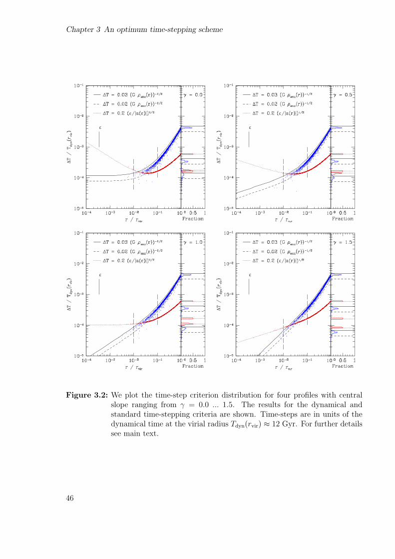
Chapter 3 An optimum time-stepping scheme
Figure 3.2: We plot the time-step criterion distribution for four profiles with centralslope ranging from γ = 0.0 ... 1.5. The results for the dynamical andstandard time-stepping criteria are shown. Time-steps are in units of thedynamical time at the virial radius Tdyn(rvir) ≈ 12 Gyr. For further detailssee main text.
46

3.3 Time-stepping criterion tests and behaviour
the add-up scheme is generally more conservative for the choice of time-step at a givenradius than the analytical value. In the two flat cases (γ = 0.0 and γ = 0.5), the binat 10−2 rvir is close to the resolution limit of the halo and the distribution is thereforequite noisy and relatively broad. Most of the effect due to this broader distribution atsmall radii is absorbed by the block time-step scheme’s way of discretizing the actualtime-step taken (see also equation 3.4); the time-step value provided by the criterion isjust an upper limit.
With a rather conservative choice of ηD = 0.03, we sample the orbit of a particle ona circular (tangential) orbit with at least 2π/ηD ≈ 200 steps. The second curve (shortdashed) used a value of ηD = 0.02 which corresponds to 2π/ηD ≈ 300 steps per circularorbit.
The situation is a bit more complicated for particles on perfect radial orbits. Fora homogeneous sphere, the particle will oscillate through the centre of the sphere anddescribe therefore a harmonic oscillator with period T =
√3π/(Gρ) where ρ is the
homogeneous density of the sphere.3 If we take this value with ρenc = ρ we get for acomplete radial orbit between
√3π/0.03 ≈ 100 and
√3π/0.02 ≈ 150 steps per oscilla-
tion. Since our time-step criterion is very adaptive with radius, the dynamical time willdecrease in a steep density profile when the particle approaches the centre, so that theeffective number of steps is even higher.
The main disadvantage of the standard time-step criterion (3.25) is the bad adaptivitywith radius, i.e. the particles are distributed over relatively few rungs. Especially inthe profile with γ = 1.0, the particles inside about ten per cent of the virial radius areall on the same time-step. For flatter central profiles with γ < 1 where ρ(r) ∝ r−γ, thetime-steps even increase inside the radius where the acceleration has its maximum, inclear contradiction to the behaviour of the dynamical time! With the asymptotic scalingof the cumulative mass function under spherical symmetry in the central region
M(r) ≡ 4π
∫ r
0
ρ(r)r2dr ∝ r3−γ (γ < 3) , (3.29)
we can calculate the asymptotic radial behaviour in the central region of the standardtime-stepping criterion
∆TS ∝√
1
|a(r)| ∝√
r2
M(r)∝ r
γ−12 (γ < 3) , (3.30)
where γ is the inner slope of the density profile, i.e. ρ(r) ∝ r−γ. In contrast, thedynamical time-stepping scheme has the following dependence
∆TD ∝√
r3
M(r)∝ r
γ2 (γ < 3) . (3.31)
3Note that Binney and Tremaine [15] defines the dynamical time as the time needed by the particleto reach the centre which means Tdyn ≡ 1
4T =√
3π/(16Gρ).
47

Chapter 3 An optimum time-stepping scheme
The standard criterion can only obtain the correct choice of time-step in the centralregions by shifting the above relation, either by choosing a small softening for theseparticles, or by reducing ηS. This automatically leads to an immense computationalexpense due to the overly conservative time-steps in the outer parts of the halo oreven wrong physical behaviour due to the choice of too small softening for the physicalproblem (e.g. undesired scattering of particles). The radial scaling of the standardcriterion makes it ill suited to the study of the centre of galaxies and in other situationswhere a very large dynamic range in density needs to be evolved correctly. The dynamicaltime-stepping technique we present is a much more universal approach to choosing time-steps in self-gravitating systems, since the basic parameters of the method, such as theangle for adding up mass contributions, once determined, are kept fixed for differentsimulations.
3.3.2 Elliptic 2-body orbits
In order to quantify the performance of our adaptive dynamical time-stepping criterionin the scattering regime, we performed a series of simulations studying the behaviour ofhigh eccentricity 2-body Kepler orbits. After choosing the masses M1 and M2 of the twobodies, all other quantities are fixed, i.e. the orbital time of the Kepler orbit is given by,
TK ≡√
a3(2π)2µ
GM1M2
= 2π
√a3
G(M1 + M2)(3.32)
and the initial total energy is calculated by,
E0 ≡ −GM1M2
2a. (3.33)
We chose a unit system where Newton’s gravitational constant G ≡ 1 and we fix theorbit in the same way, i.e. the semi-major axis is always a ≡ 1. The softening ε ofthe two particles was set to 0.1 dperi in all cases where dperi ≡ a(1 − e) is the periapsisdistance of the Kepler orbit. PKDGRAV treats the forces completely Newtonian if thetwo particles have a distance larger than 2ε which is therefore always the case in thesetest runs. Initially, the particles were set in a coordinate system where the centre ofmass is at rest at the origin and the two particles were at apoapsis configuration alongthe x-axis. A short summary of the parameters can be found in table 3.2.
We let each run evolve for 1000 TK (TK was also the basic or longest time-step in theblock time-stepping scheme, T0), measured the total energy E1000 after the end of therun and calculated the relative energy shift (E1000 − E0)/|E0|. These values are alsolisted in table 3.2. From table 3.2, we see that even for a high eccentricity (e = 0.999)orbit we still have relative energy conservation on the level of ≈ 10−6 per orbit. Thegeneral behaviour can also be seen in figure 3.3 where we plot the orbit from 0 to TK
and the orbit from 999 TK to 1000 TK for each of the different runs i) - l). The twoorbits lie nearly on top of each other except for the e = 0.99 case, where the energy gainin the integration was the largest, we can see a small deviation. When we compare the
48

3.3 Time-stepping criterion tests and behaviour
Figure 3.3: Top left: run i), top right: run j), bottom left: run k), bottom right: run l)from table 3.2. We plot the orbit from 0 to TK (orbit 1) and the orbit from999 TK to 1000 TK (orbit 1000) for each run. All runs used the dynamicaltime-stepping scheme with eccentricity correction. We deliberately did notplot the scaling of the two axes constrained in order to make the smalldeviations visible.
49

Chapter 3 An optimum time-stepping scheme
Figure 3.4: Top left: run b), top right: run m), bottom left: run n), bottom right:run o) from table 3.2. Run b) shows the dynamical time-stepping casewith eccentricity correction. The orbit is perfectly followed. In run m), wecan nicely see the energy gain visually due to the lack of the eccentricitycorrection in the time-step criterion. Run n) where we tried to resolve ae = 0.9 orbit analogue to run b) with the standard time-step criterion. Inrun o), we see a run where we used a smaller value of ηS = 0.029 so thatthe standard criterion initially makes an equal number of steps per orbitas the dynamical time-stepping scheme in run b). For further details seemain text.
50

3.3 Time-stepping criterion tests and behaviour
Figure 3.5: Run p) where we tried to resolve an e = 0.9, high mass ratio orbit withthe standard time-stepping criterion. The heavy particle gets an immensekick and the total energy becomes positive. Thus, the heavy particle dragsthe light particle with it and the whole system drifts apart. The standardcriterion therefore fails completely to follow the orbit correctly.
runs with different mass ratios, we see that the relative energy conservation is nearly thesame, i.e. the relative energy conservation depends only on the geometry of the orbit.
In order to illustrate the robustness of our method we have performed some furthertests. In run m), we switched off the eccentricity correction in the symmetrised dynam-ical time-stepping (3.22), i.e. C(e) = 1. We see that the energy gain over 1000 TK is≈ 240 times larger than in the corresponding run b) with eccentricity correction. Thiscan also be seen visually in figure 3.4. Due to the energy gain, the orbits of both particlesbecome wider.
In run n) we tried to resolve the orbit with the standard time-stepping criterion givenby equation (3.25). This criterion depends on the softening length ε of the particle andis therefore certainly not ideal in the gravitational scattering regime. We’ve chosen thesame value as in run b) where we had ε = 0.1 dperi = 0.01. From figure 3.4 we seeimmediately when comparing run n) and b) that the standard criterion can not capturethe dynamics of the orbit. The orbits of the two particles become more circular and weget a rotation of the whole system. If we had chosen a somewhat larger softening, sothat it is still smaller than half the periapsis distance, it would even look worse sincethe standard time-stepping scheme directly depends on the softening length ε while thedynamical time-stepping scheme would still perform equally well since it has no suchdependence.
Of course, the dynamical time-stepping criterion with eccentricity correction uses alot more steps per orbit than the standard criterion with ηS = 0.2. Therefore we tried
51

Chapter 3 An optimum time-stepping scheme
Figure 3.6: The most extreme case, run I), with mass ratio of 106 and eccentricity e =1.001. The dynamical time-stepping scheme with eccentricity correctionis used. There is no significant evolution over 1000 repeated pericentrepassages.
in run o) a run with an equal number of steps per orbit as run b). This is reached fora value η = 0.029. The energy conservation is still not as good as in the case of thedynamical time-stepping with eccentricity correction b) and there is a small amount ofprecession of the periapsis.
The whole situation becomes even worse when we try to resolve 2-body orbits withunequal mass particles. Since the standard time-stepping is not symmetric due to theasymmetry in acceleration, it is not able to resolve a high mass ratio 2-body orbitcorrectly and fails completely. This is shown in figure 3.5. Although the light particlemakes N = 3197 steps in the first orbit (here N in run p) denotes only the number ofsteps of the light particle in table 3.2), the heavy particle takes a much larger first stepthan the light particle. Of course when then the light particle approaches, the heavyparticle gets an immense kick, the total energy becomes positive and the whole systemdrifts apart.
3.3.3 Hyperbolic 2-body orbits
In a similar way, we also tested the new dynamical time-stepping scheme for hyperbolicorbits. Initial conditions were set up such that the line connecting the two particlesencloses an angle of π
6with the semi-major axis (symmetry axis) of the hyperbola. The
time for the particle to reach the periapsis of the orbit is given by
TH =
∫ π
π6
µ r2(φ)
Ldφ (3.34)
52
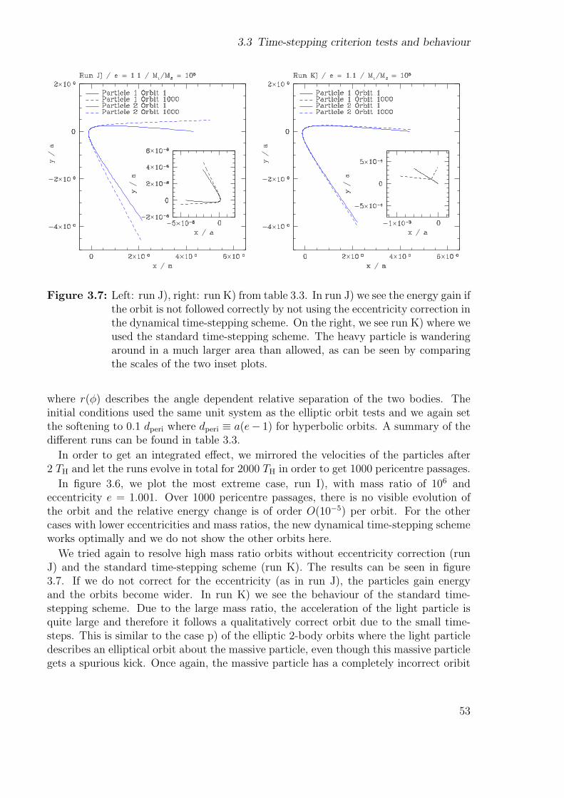
3.3 Time-stepping criterion tests and behaviour
Figure 3.7: Left: run J), right: run K) from table 3.3. In run J) we see the energy gain ifthe orbit is not followed correctly by not using the eccentricity correction inthe dynamical time-stepping scheme. On the right, we see run K) where weused the standard time-stepping scheme. The heavy particle is wanderingaround in a much larger area than allowed, as can be seen by comparingthe scales of the two inset plots.
where r(φ) describes the angle dependent relative separation of the two bodies. Theinitial conditions used the same unit system as the elliptic orbit tests and we again setthe softening to 0.1 dperi where dperi ≡ a(e− 1) for hyperbolic orbits. A summary of thedifferent runs can be found in table 3.3.
In order to get an integrated effect, we mirrored the velocities of the particles after2 TH and let the runs evolve in total for 2000 TH in order to get 1000 pericentre passages.
In figure 3.6, we plot the most extreme case, run I), with mass ratio of 106 andeccentricity e = 1.001. Over 1000 pericentre passages, there is no visible evolution ofthe orbit and the relative energy change is of order O(10−5) per orbit. For the othercases with lower eccentricities and mass ratios, the new dynamical time-stepping schemeworks optimally and we do not show the other orbits here.
We tried again to resolve high mass ratio orbits without eccentricity correction (runJ) and the standard time-stepping scheme (run K). The results can be seen in figure3.7. If we do not correct for the eccentricity (as in run J), the particles gain energyand the orbits become wider. In run K) we see the behaviour of the standard time-stepping scheme. Due to the large mass ratio, the acceleration of the light particle isquite large and therefore it follows a qualitatively correct orbit due to the small time-steps. This is similar to the case p) of the elliptic 2-body orbits where the light particledescribes an elliptical orbit about the massive particle, even though this massive particlegets a spurious kick. Once again, the massive particle has a completely incorrect oribit
53
Chapter 3 An optimum time-stepping scheme
wandering around in a very large area due to the spurious kicks (compare the scales ofthe inset plots in runs J and K). The lack of momentum conservation in such cases resultsin this contrasting behaviour of the two different mass particles. The symmetrizationof the time-step criterion restores momentum conservation between the two particlesinvolved in the gravitational scattering event.
3.3.4 Cosmological structure formation
We also tested the performance of the dynamical time-stepping scheme in a cosmologicalstructure formation run. For this purpose, we used a fiducial simulation of the Virgocluster [61] in a cosmological framework with ΩM = 1, no cosmological constant i.e.ΩΛ = 0 and H0 = 50 km s−1 Mpc−1. The simulation cube had a box length of L =100 Mpc and the total mass in the cube was Mtot = 6.937 × 10¹⁶ M¯. The clusterwas resolved using the standard refinement technique [77, 78] so that the particle massin the highest resolution region was 8.604 × 10⁸ M¯ and the softening length of thelightest particles was ε = 5 kpc. The total number of particles was 1.314 × 10⁶. Thesimulation started at redshift z = 69 and we evolved the cluster to redshift z = 0 withthree different time-stepping schemes: one dynamical and one standard time-steppingrun and, for comparison, a fixed time-step scheme with 300000 time-steps from z = 69 toz = 0 (this corresponds to 20000 time-steps down to redshift z = 5 in the above describedcosmology). With this choice, the fixed time-step length corresponds approximately tothe smallest time-step chosen by the dynamical criterion during the whole run. Onlyfor a few particles, the dynamical scheme did choose smaller steps than this fixed time-stepping run.
The virial radius of the resulting cluster was in all cases rvir ≈ 2 Mpc (overdensity ≈200) and had a final mass of MCluster ≈ 4.3× 10¹⁴ M¯. In figure 3.8, we plot on the toppanel the radial density profile for the three runs at redshift z = 0. Here ρD(r) is theradial density of the run with the dynamical time-stepping scheme, ρS(r) the densityprofile of the run with the standard time-stepping scheme and ρF(r) the profile of thefixed time-step run. In the lower panel, the relative difference (ρ(r) − ρF(r))/ρF(r) isalso plotted. The softening of the highest resolution particles correspond to ε = 5 kpc ≈2.5 × 10⁻³ rvir. As we can see in figure 3.8, the same radial density profile is obtainedfor the final cluster in this cosmological simulation.
We also compared the substructure mass function at redshifts z = 0 and z = 5 for thethree runs. For that, we used the group finding software skid4 with a linking length of20 kpc = 4 ε and a density and number cut so that only structures that are virialised andwhich are represented by at least 100 particles are accepted. In figure 3.9, we plot themass function n(M) (number of substructures of mass M) as a function of substructuremass M for output at redshifts z = 5 and z = 0. There is no substantial differencebetween the mass functions for the different time-stepping schemes.
For these low resolution runs we do not expect to see a significant difference betweenthe three runs since the scale at which the standard scheme begins to take an insufficient
4www-hpcc.astro.washington.edu/tools/skid.html
54

3.3 Time-stepping criterion tests and behaviour
Figure 3.8: Density profiles of the three runs of the Virgo cluster with the differenttime-stepping schemes at final redshift z = 0: ρD(r) is the radial density ofthe run with the dynamical time-stepping scheme, ρS(r) the density profileof the run with the standard time-stepping scheme and ρF(r) the profileof the fixed time-step run. The profiles are normalised with respect to thecritical density ρcrit. On the top panel, the absolute values and on the lowerpanel the relative differences (ρ(r)− ρF(r))/ρF(r) are plotted.
55

Chapter 3 An optimum time-stepping scheme
Figure 3.9: Substructure mass function of the Virgo cluster run at redshift z = 5 (left)and z = 0 (right). There is no substantial difference between the runs withdifferent time-stepping schemes visible.
number of time-steps corresponds approximately to the resolution scale of this simula-tion. This is just a confirmation that the dynamical time-stepping scheme also worksfor the extreme dynamics of a cosmological structure formation run.
3.3.5 Dependence on parameters
Softening length ε
The standard time-step criterion (3.25) depends directly on the artificial simulationparameter softening length ε. There is however no physical basis for this definition.Furthermore, the functional form of the acceleration in centrally flat (γ < 1) haloes isproblematic and can lead to nonsensical time-steps if the resolution is high enough (seefigure 3.2). Even a simple 2-body problem is not treated properly by the standard time-stepping scheme, since the time-steps depend on acceleration which is not symmetricand again there is the meaningless dependence on the softening of the particles.
The dynamical time-stepping scheme only depends indirectly on the softening length.If two particles are close enough such that their forces are softened, we also use thesoftened values for the ρenc. In this way the scheme also determines an appropriatedynamical time-step when the Green’s function deviates from the Newtonian 1/r. Fur-thermore, the new dynamical time-stepping scheme may be used without modificationin simulations where the softening is set to zero, i.e., where the interactions are neversoftened.
56
3.3 Time-stepping criterion tests and behaviour
Force opening angle θ
The opening angle θ determines the weighting of directly calculated forces to force con-tributions coming from the multipole expansion. This parameter mainly determines theaccuracy of the force. By including the terms in the particle-bucket list, the dynamicalscheme does not show a significant dependence on the choice of the force opening angleθ.
Cone viewing angle α
We normalised the viewing angle α so that the volume of the sphere and the cone infigure 3.1 are equal. We also tried larger values of cos(α) > 0.75 (i.e. smaller angles)but the resulting time-step distribution did not follow the theoretical curves as well asfor the case of cos(α) = 0.75 (especially close to the centre).
Number of maxima
Ideally, one would scan the particle’s whole sky for the gravitationally dominating struc-ture. But this would be computationally very expensive. With our choice of the 0.5percentile largest ρenc cells in each of the cell and particle-bucket lists we find a goodcompromise between getting the correct dominating structure (i.e. low scattering of theenclosed density values) and computational speed. Having to consider multiple maximais the main factor which makes the dynamical time-stepping scheme more expensive thanthe simple schemes used to-date. However, if we loosen the strict geometrical definitionof the viewing cone, then faster schemes which rely on the hierarchical tree structurewhen scanning the sky for maxima and their surrounding mass become realisable. Suchalgorithmic improvements are being investigated and will be discussed in future work.
Prefactor ηD
Stadel [144] performed stability tests for a leapfrog scheme in the drift-kick-drift mode.The result was that 2-body orbits became unstable for choices of ηD ≥ 0.1. For thesetests, the choice of time-steps was also based on the dynamical time of the 2-bodyproblem.
We performed similar tests with the kick-drift-kick leapfrog scheme and found thate = 0.9 orbits become unstable in the mean field regime (i.e. without eccentricitycorrection) for choices of ηD too large. Of course by choosing a smaller value of ηD, onealways gets better precision but the computational costs become larger. With the choiceof ηD = 0.03 we found a compromise between stability and computational costs.
3.3.6 Efficiency
In order to quantify the efficiency of the dynamical time-stepping criterion in comparisonwith the standard criterion, we can compare the number of force evaluations for a given
57

Chapter 3 An optimum time-stepping scheme
problem. In a spherically symmetric halo, the number of particles in a shell at radius rwith thickness dr is given by
dNP =4πρ(r)r2dr
Mvir/Nvir
. (3.35)
The number of time-steps per time interval τ for each of these dNP particles at radius ris given by
ND =τ
ηD
√Gρenc(r) =
τ
ηD
√GM(r)
r3(3.36)
in the dynamical case. In the case of the standard time-stepping scheme, this is insteadgiven by
NS =τ
ηS
√|a(r)|
ε=
τ
ηS
√GM(r)
ε r2. (3.37)
We do not account for the actual block time-stepping scheme used in PKDGRAV forthis numerical estimation.
The number of force evaluations in that infinitesimal thin shell is now simply givenby
dFS = dNP NS (3.38)
respectivelydFD = dNP ND . (3.39)
The ratio
RE ≡ dFS
dFD
=ηD
ηS
√r
ε, (3.40)
shows that above req defined by equation (3.28), i.e. the radius where both time-steppingcriteria give the same value, the number of force evaluations at a given radius is alwaysa factor RE ∝
√r larger.
In figure 3.10, we plot the number of force evaluations per Gyr per radius dFD/dr anddFS/dr for a dark matter halo with central profile γ = 1.0 used also in figure 3.2 withNvir = 7.5× 10⁶. The figure shows the asymptotic behaviour of the curves in the centralregion given by
dFD
dr∝ r2− 3
2γ γ=1∝ r
12 (3.41)
respectivelydFS
dr∝ r
52− 3
2γ γ=1∝ r1. (3.42)
In the inner region, i.e at distances smaller than req from the centre, more force evalua-tions are done in the dynamical time-stepping scheme, as expected. Here the standardscheme does not give small enough time-steps to follow the dynamics. Since in mostcases of low resolution simulations req (due to a clever choice of softening or ηS) is aroundthe resolution scale, the error is typically small. High resolution simulations can howeverbecome very slow if one wants to resolve the central region correctly with the standardtime-stepping scheme.
58

3.3 Time-stepping criterion tests and behaviour
Figure 3.10: Number of force evaluations N per Gyr per radius for the dynamicalscheme dFD/dr respectively dFS/dr for the standard scheme for a darkmatter halo with central profile γ = 1.0. For infinitesimal thin shellsat radii larger than req, the standard time-stepping scheme has alwaysa factor RE (given by equation (3.40)) more force evaluations per Gyr.The inner slope is γ = 1 and we have therefore the following asymptoticbehaviour in the centre: dFD/dr ∝ r
12 and dFS/dr ∝ r1.
59

Chapter 3 An optimum time-stepping scheme
Nvir 7.5× 10⁶ 7.5× 10⁸ 7.5× 10¹⁰
FD 7.612× 10⁸ 7.612× 10¹⁰ 7.612× 10¹²
FS 2.336× 10⁹ 7.388× 10¹¹ 2.336× 10¹⁴
FS
FD3.069 9.705 30.69
Table 3.1: Number of force evaluations per Gyr for an halo with γ = 1.0 and differentresolutions Nvir.
In order to illustrate the efficiency gain, we calculate the number of force evaluationsper Gyr for three different haloes with central slope γ = 1.0 that have the same profileand specifications as the one used in figure 3.2 and 3.10. We only changed the numberof particles: they are Nvir = 7.5× 10⁶, 7.5× 10⁸ and 7.5× 10¹⁰ particles within the virialradius. For the first halo we chose a softening length of ε1 = 100 pc ≈ 3.5 × 10⁻⁴ rvir
and we scaled the softening of the other haloes according to the scaling of rimp given bythe solution of
rimp = h(rimp) , (3.43)
where h(r) is the mean particle separation defined by
h(r) ≡ 3
√Mvir/Nvir
ρ(r). (3.44)
Seee also section 2.1 for further details. In other words, rimp is the distance of theinnermost particle to the geometrical centre of the halo and scales as
rimp ∝ 3−γ
√1
Nvir
γ=1∝√
1
Nvir
(3.45)
resulting in ε2 = 10 pc and ε3 = 1 pc for the other softenings.The number of force evaluations per Gyr (τ = 1 Gyr) is given by
FD =
∫ rvir
rimp
dFD respectively FS =
∫ rvir
rimp
dFS , (3.46)
and the numerical results can be found in table 3.1. We see that FD scales as FD ∝ Nvir
whereas FS scales approximately as FS ∝ N1.25vir in the case of a halo profile with γ = 1.0.
This specific scaling of FS is due to the scaling of the softening length ε ∝ rimp resultingin the general scaling of
FS ∝ N1+ 1
2(3−γ)
vir . (3.47)
For a different scaling of the softening, one gets of course a different scaling of FS,e.g. ε ∝ N
−1/3vir results in FS ∝ N
7/6vir independent of γ. This again shows the strong
dependence of the standard scheme on the softening length ε and that the the dynamicaltime-stepping scheme is much more efficient than the standard scheme for high resolutionsimulations.
60

3.4 Conclusions
3.4 Conclusions
We have developed a physically motivated time-stepping scheme that is based on the truedynamical time of the particle. We also derive an eccentricity correction for a generalleapfrog integration scheme. The combination of these schemes allows us to follow quitegeneral dynamical systems that may contain a mixture of collisionless and collisionalinteracting components. Compared to the standard time-stepping scheme used in manyN-body codes it has the following advantages:
• It does not depend directly on ad-hoc parameters such as the softening length ε.
• It gives physically correct time-steps in dark matter haloes with arbitrary centralcusp slopes.
• It is faster in high resolution simulations.
• It allows orbits with eccentricity e → 1 to be followed correctly.
• It allows us to follow complex dynamical systems where scattering events may beimportant.
The main conclusion is that one should use a time-step criterion that is based on thedynamical time. This scheme shows the optimum scaling with the number of particlesand always gives a physically motivated time-step.
61

Chapter 3 An optimum time-stepping scheme
Run
M1/M
2e
TK
E0
(E1000−
E0)/|E
0|
Nti
me-
step
pin
gsc
hem
eco
mpar
ew
ith
run
a)1
04.
443
−5×
10−1
2.23
8×
10−9
256
D/
ecb)
10.
94.
443
−5×
10−1
−7.2
78×
10−4
2110
D/
ecm
),n),
o)c)
10.
994.
443
−5×
10−1
6.64
8×
10−3
9394
D/
ecd)
10.
999
4.44
3−5
×10−1
2.80
4×
10−3
3914
3D
/ec
e)10
30
1.98
5×
10−1
−5×
102
2.25
4×
10−9
256
D/
ecf)
103
0.9
1.98
5×
10−1
−5×
102
−7.0
14×
10−4
2110
D/
ecg)
103
0.99
1.98
5×
10−1
−5×
102
6.64
8×
10−3
9394
D/
ech)
103
0.99
91.
985×
10−1
−5×
102
2.80
4×
10−3
3914
2D
/ec
i)10
60
6.28
3×
10−3
−5×
105
2.24
2×
10−9
256
D/
ecj)
106
0.9
6.28
3×
10−3
−5×
105
−7.2
18×
10−4
2110
D/
ecp)
k)
106
0.99
6.28
3×
10−3
−5×
105
6.65
3×
10−3
9394
D/
ecl)
106
0.99
96.
283×
10−3
−5×
105
2.80
2×
10−3
3914
2D
/ec
m)
10.
94.
443
−5×
10−1
1.73
0×
10−1
398
D/
nec
b)
n)
10.
94.
443
−5×
10−1
−1.2
6331
6S
b)
o)1
0.9
4.44
3−5
×10−1
1.89
5×
10−3
2107
S/
η S=
0.02
9b)
p)
106
0.9
6.28
3×
10−3
−5×
105
1.91
331
97S
j)
Table
3.2
:Sum
mar
yof
ellipti
c2-
body
orbit
runs
a)-
p).
The
colu
mns
are
mas
sra
tio
M1/M
2,ec
centr
icity
e,or
bit
alti
me
TK,in
itia
len
ergy
E0,re
lati
veen
ergy
chan
ge(E
1000−
E0)/|E
0|,
num
ber
ofst
eps
duri
ng
the
firs
tor
bit
N,ti
me-
step
pin
gsc
hem
e:D
-dynam
ical
,S
-st
andar
d,ec
-ec
centr
icity
corr
ecti
on,nec
-no
ecce
ntr
icity
corr
ecti
on,ru
nto
com
par
ew
ith:
b)
wit
hm
),n)
and
o)an
dj)
wit
hp).
62

3.4 Conclusions
Run
M1/M
2e
TH
E0
(E1000−
E0)/|E
0|
Nti
me-
step
pin
gsc
hem
eco
mpar
ew
ith
run
A)
11.
12.
150
5×
10−1
3.00
9×
10−3
1713
D/
ecB
)1
1.01
2.27
4×
10−2
5×
10−1
2.11
9×
10−3
4935
D/
ecC
)1
1.00
16.
709×
10−4
5×
10−1
−1.2
98×
10−2
1517
7D
/ec
D)
103
1.1
9.61
0×
10−2
5×
102
3.00
9×
10−3
1713
D/
ecE
)10
31.
011.
017×
10−3
5×
102
2.11
9×
10−3
4935
D/
ecF)
103
1.00
12.
999×
10−5
5×
102
−1.2
98×
10−2
1517
8D
/ec
G)
106
1.1
3.04
1×
10−3
5×
105
3.00
9×
10−3
1713
D/
ecJ),
K)
H)
106
1.01
3.21
6×
10−5
5×
105
2.11
8×
10−3
4935
D/
ecI)
106
1.00
19.
488×
10−7
5×
105
−1.2
98×
10−2
1517
7D
/ec
J)
106
1.1
3.04
1×
10−3
5×
105
8.33
6×
10−1
296
D/
nec
G)
K)
106
1.1
3.04
1×
10−3
5×
105
1.36
0×
10−1
333
SG
)
Table
3.3
:Sum
mar
yof
hyper
bol
ic2-
body
orbit
runs
A)
-K
).T
he
colu
mns
are
mas
sra
tio
M1/M
2,ec
centr
icity
e,ti
me
tore
ach
the
per
icen
tre
TH,in
itia
len
ergy
E0,re
lati
veen
ergy
chan
ge(E
1000−
E0)/|E
0|,
num
ber
ofst
eps
duri
ng
the
firs
tor
bit
N,ti
me-
step
pin
gsc
hem
e:D
-dynam
ical
,S
-st
andar
d,ec
-ec
centr
icity
corr
ecti
on,nec
-no
ecce
ntr
icity
corr
ecti
on,ru
nto
com
par
ew
ith:
G)
wit
hJ)
and
K).
63

Chapter 3 An optimum time-stepping scheme
64

Chapter 4
Applications
The development of the multi-mass technique and especially the time-stepping schemewere very time consuming. The author of this thesis was therefore involved in the firstapplication projects that used these new developments as a co-author. In Diemand et al.[38], the the multi-mass technique was used in a cosmological structure formation runin order to resolve the resulting density profile of a high resolution cluster down to oneper mill of the virial radius. Goerdt et al. [64] used multi-mass models in order to testa potential explanation of the presence of the five globular clusters at approximately 1kpc distance form the centre of the Fornax dwarf spheroidal galaxy. In this chapter wepresent a summary of these projects.
4.1 Cusps in cold dark matter haloes1
4.1.1 Introduction
Recently a great deal of effort has gone into high resolution simulations which haverevealed density profiles of cold dark matter haloes down to scales well below one per centof the virial radius [34, 54, 117, 129, 149]. But the form of the profile below approximately0.5 per cent of the virial radius remained unclear and there was no clear evidence fora cusp in the centre, i.e. no significant inner region with a constant logarithmic slope.Galaxy cluster haloes would be the ideal systems to resolve cusps numerically becauseof their low concentration. In a galaxy or dwarf halo the inner power law is much harderto resolve because it lies at a smaller radius relative to the size of the system.
The existence of a core or a cusp in the centre of cold dark matter haloes has impor-tant observational consequences and is the crucial point in many tests of the cold darkmatter theory. Comparisons of dark matter simulations to rotation curves of low sur-face brightness galaxies seem to favour constant density cores for most observed systems[28, 48, 107, 134, 139, 148, 157]. But these comparisons still depend to some extent onextrapolations of the simulated profiles toward the centre: Stoehr [145] extrapolate toa constant density core and claim that the discrepancy to low surface brightness galaxyrotation curves is much smaller than previously believed.
The strength of the γ-ray signal from dark matter annihilation depends on the squareof the dark matter density and the calculated flux values spread over several orders of
1Original publication: MNRAS, 364, 665 (2005) [38]
65
Chapter 4 Applications
magnitude, depending on how one extrapolates the density profiles from the known,resolved regions down into the centres of the galactic halo and its subhaloes [12, 18, 126,146]. Small, very abundant, Earth to Solar mass subhaloes could be very luminous inγ-rays if they are cuspy [37].
The highest resolutions in cosmological simulations are reached with the widely usedrefinement procedure [13]: first one runs a simulation at uniform, low resolution andselects haloes for re-simulation. Then one generates a new set of initial conditionsusing the same large scale fluctuations at higher resolution and additional small scalefluctuations in the selected region. With this technique Navarro et al. [116] were able toresolve many haloes with a few ten thousand particles and to infer their average densityprofile which asymptotes to an ρ(r) ∝ r−1 cusp. Other authors used fitting functionswith steeper (ρ(r) ∝ r−1.5) cusps [52, 62, 110, 112]. Small mass cold dark matter haloeshave higher concentrations due to their earlier collapse [116] but the slopes of the innerdensity profiles are independent of halo mass [27, 113]. Open, standard and lambda colddark matter (ΛCDM) cosmologies, i.e. models with (ΩM,ΩΛ) = (0.3, 0.0), (1.0, 0.0) and(0.3, 0.7) yield equal inner profiles [53, 54]. There is some indication that models withless small scale power like warm dark matter lead to shallower inner profiles [26, 129].Different equations of state of the dark energy component lead to different collapse timesand halo concentrations but it is not clear yet if it also affects slopes well inside of thescale radius [86, 92]. Most current simulations do not resolve a large enough radial rangeto determine both the concentration and the inner slope; at the current resolution theseparameters show some degeneracy [84].
Recently a large sample of ΛCDM haloes resolved with a million and more particles wassimulated [57, 117, 129, 142, 149] and the best resolved systems contain up to 25 millionparticles [34, 54]. But even these very large, computationally expensive simulationsresolved no inner region with a constant logarithmic slope.
Navarro et al. [117], Stoehr [145], Stoehr et al. [146] introduced cored profiles whichseem to fit the simulation data better than the cuspy profiles proposed earlier by Navarroet al. [116] and Moore et al. [112]. This better fit was interpreted as indication againstcuspy inner profiles. However these cored profiles have one additional parameter andtherefore it is not surprising that they fit the data better. Diemand et al. [34] showed thatan αβγ-profile (see equation (2.1)) with the inner slope as additional free parameter fitsthe highest resolution profiles just as well as cored profiles. Some theoretical argumentsseem to favour cusps [14, 67] but make only vague predictions about the inner slopes. Arecent model combines simulation results and analytical arguments to predict an innerslope of -1.27 [6]. At the moment higher resolution simulations seem to be the only wayto decide the core versus cusp controversy.
We present simulations of one of the galaxy clusters from Diemand et al. [34] withtwo orders of magnitude better mass resolution. Our results give strong support tocuspy inner profiles. This increase in resolution was made possible with only a moderateincrease in computational cost by using the multi-mass refinement technique (see section2).
66

4.1 Cusps in cold dark matter haloes
Name D5 D12 DM25 DM50N eff
vir 1.0× 10⁶ 1.4× 10⁷ 1.3× 10⁸ 1.0× 10⁹
Multi-mass refinement no no yes yeszStart 52.4 43.3 52.4 59.3zEnd 0 0 0.8 4.4
Table 4.1: Summary of cluster models. The rows are effective number of particleswithin virial radius N eff
vir, application of multi-mass refinement, start redshiftzStart and end redshift zEnd.
4.1.2 Numerical methods
Often in cosmological N-body simulations one uses high resolution particles only whereone halo forms and heavier particles in the surroundings to account for the external tidalforces. One usually tries to define a large enough high resolution region to minimize oravoid mixing of different mass particles within the region of interest. Here we apply themulti-mass technique to increase the resolution in the centre of one cluster halo in acosmological N-body simulation.
The refinement procedure is usually applied to entire virialised systems, i.e. onemarks all particles inside the virial radius of the selected halo and traces them backto the initial conditions. Then one refines the region that encloses the positions of themarked particles. Usually the region is further increased to prevent any mixing of lowresolution particles into the virial radius of the final system. But with this procedureonly between one fourth to one third of all the high resolution particles end up in thecluster.
If one is only interested in the inner regions of a halo it is possible to use the multi-mass technique: instead of refining the whole virialised system we only refine the regionwhere the inner particles come from. This allows to reduce the size of the high resolutionregion considerable, because most of particles that end up near the centre of the systemstart in a very small region, compared to the region which one finds by tracing backall the particles inside the virial radius. Using this technique it is possible to reducethe computational cost of a cold dark matter cluster simulation by at least one order ofmagnitude at equal force and mass resolution in the inner region.
Here, we applied the multi-mass refinement to the cluster D from Diemand et al. [34].This cluster is well relaxed and isolated at z = 0 and has an average density profileand inner slope close to the mean value. First we marked all particles within one percent of the virial radius in the final halo and traced them back to the initial conditions.Then we added all particles within one comoving Mpc of a marked particle to the set ofmarked particles, and finally we added all particles which lie on intersections of any twoalready marked particles on the unperturbed initial grid positions. After these two stepsthere was a region with a fairly regular triaxial boundary which contained only markedparticles. The number of marked particles grew by almost a factor of eight during theseadditions, but it was still more than a factor of two smaller than the number of particlesin the final cluster and a factor of ten smaller than the original high resolution volume
67

Chapter 4 Applications
used in Diemand et al. [34].With an effective mass resolution corresponding to 1.3 × 10⁸ and 1.0 × 10⁹ particles
inside the virial radius of a cluster, the models DM25 and DM50 are the highest resolu-tion ΛCDM simulation performed so far. Due to the large number of particles and thecorresponding high force and time resolution these runs took a large amount of run time.Fortunately the inner profiles of cold dark matter clusters are already in place aroundredshift z = 1 and evolve little between z = 4 and z = 0 [54, 129, 149]. Therefore onedoes not have to run the simulations to z = 0 to gain insight into the inner densityprofile. We stop DM50 at z = 4.4, DM25 at z = 0.8 and use the medium resolutionruns D5 and D12 (for which the multi-mass technique was not applied) to quantify thelow redshift evolution of the density profile of the same cluster. The D5 model has aresolution of 1.0 × 10⁶ particles and the D12 version was resolved with 1.4 × 10⁷ equalmass particles.
All the runs were evolved with PKDGRAV (see section 1.3.5) from redshift zStart tozEnd given in the summary of the models in table 4.1.
4.1.3 Results
Run DM25 had an effective resolution corresponding to 127 million particles within thevirial radius and a softening length of 0.48 × 10⁻³ rvir. At this up to now unmatchedresolution the inner slope is roughly constant from the resolved radius (see figure 4.1)out to about one per cent of the virial radius of the final cluster. Run D12 resolved thesame cluster with 14 million particles and showed no convergence to a constant innerslope. This indicates that there is a cusp in the centres of cold dark matter clustersand it becomes apparent only at this very high numerical resolution. The non-constantslopes just near the convergence scale are probably due to the first signs of numericalflattening that set in at this scale. At higher densities below the resolved scales onecannot make any robust predictions yet, but if one has to extrapolate into this regionfigure 4.1 motivates the choice of a cusp ρ(r) ∝ r−γ with γ ' 1.2.
Mass accretion histories show that the inner part of cold dark matter haloes is assem-bled in an early phase of fast accretion [156, 163, 175] and recent high resolution simula-tions revealed that the inner density profile does not evolve at low redshift [54, 129, 149].Figure 4.1 confirms that the inner density profile of runs D12 does not change fromz = 0.8 to z = 0.
Therefore in run DM50 we focused our computational effort even more on the earlyevolution of the inner profile. We refined the inner region of the most massive progenitoridentified in run DM25 at z = 4.4. Since the refinement region needed is much smallerthan the one of DM25 and we only ran the simulation to z = 4.4, it is feasible to go to amuch better mass and force resolution. The high resolution particles in run DM50 werea billion times lighter than the final cluster.
Figure 4.2 shows that the density profile of run DM50 at z = 4.4 is cuspy down tothe resolved radius (one per mill of the final virial radius). As in run DM25 the slopesbegin to shallow just at the converged scale due to numerical flattening. The profile ofDM50 at z = 4.4 supports the finding from run DM25 that the inner profile follows a
68

4.1 Cusps in cold dark matter haloes
10−3
10−2
10−1
−2.2
−2
−1.8
−1.6
−1.4
−1.2
−1
−0.8
−0.6
−0.4
r / rvir
(z=0)
d lo
g ρ
(r)
/ d lo
g r
z=0.8
↓ rresolved,DM25
↓ rresolved,D12
↓ rresolved,D5
DM25D12D12 z=0D5
Figure 4.1: Logarithmic slope of the density profile of run DM25 at z = 0.8. Theslopes of runs D5 and D12 at z = 0.8 and z = 0 for D 12 are also shown forcomparison. The arrows indicates the estimated convergence radii. Notethat although the densities at the converged scales are within ten per centthe density gradients can already be substantially smaller.
69

Chapter 4 Applications
10−3
10−2
−2.5
−2
−1.5
−1
−0.5
0
r / rvir
(z=0)
d lo
g ρ
(r)
/ d lo
g r
z=4.4
↓ rresolved,DM25
↑ rresolved,DM50
↓ rresolved,D5
DM50DM25D5
Figure 4.2: Logarithmic slope of the density profile of run D5, DM25 and DM50 atz = 4.4. The arrows indicates the estimated convergence radii. A constantinner slope of about -1.2 is evident in the highest resolution run DM50.The increase of the slopes around the resolved radii is due to the onset ofnumerical flattening.
70

4.1 Cusps in cold dark matter haloes
steep power law ρ ∝ r−1.2. At the higher resolution of run DM50 we find substantiallyhigher physical densities in the cluster centre at z = 4.4 compared to lower resolutionruns like DM25. This suggests that a run like DM50 evolved to low redshift would alsoyield substantially higher central densities as currently resolved in the centres of runslike D12 and DM25.
Now we went one step further and used the information from all the D-series runs totry to estimate the density profile one would obtain if one simulates this cluster with abillion particle all the way to present time, a run which would be possible but extremelyexpensive with today’s computational resources. From figure 4.3 one finds that thedensity profile of run DM25 near its resolution scale shifts upward by a constant factorof 1.4 from z = 4.4 to z = 0.8. The density around 0.01 rvir(z = 0) is constant formz = 0.8 to z = 0, see run D5 in figure 4.3. The inner density profile slopes are constanteven longer, i.e. from z = 4.4 to z = 0, see figures 4.1 and 4.2. Therefore we estimatedthe z = 0 profile of run DM50 by rescaling the z = 4.4 profile of DM50 by a factor1.4 and using the z = 0 profile of run D12 outside of 0.005 rvir(z = 0) (see figure 4.3).The extrapolated z = 0 profile of run DM50 should be regarded as a best guess for thedensity profile of an average cold dark matter cluster resolved with a billion particles.A (multi-mass) simulation with this (effective) resolution evolved to redshift zero wouldbe needed to check the accuracy of the estimate performed here.
We fitted one cuspy and two recently proposed cored functions to the density profileof the tentative z = 0 extrapolation from run DM50. From the arguments above weexpected the cuspy function to work better in the inner part but we tried to fit also thecored profiles for comparison.
As cuspy density profile, we used a general αβγ-profile given by equation (2.1). Ifone takes α, β and γ as free parameter one encounters strong degeneracies, i.e. verydifferent combinations of parameter values can fit a typical density profile equally well[84]. Therefore we fixed the outer slope β = 3 and the turnover parameter α = 1. Wefitted the three parameters γ, rs and ρ0 to the data.
Navarro et al. [117] proposed a different fitting function which curves smoothly overto a constant density at small radii:
ln(ρN(r)/ρ0) = (−2/αN) [(r/rs)αN − 1] (4.1)
αN determines how fast this profile turns away from a power law in the inner part.Navarro et al. [117] found that αN is independent of halo mass and αN = 0.172± 0.032for all their simulations, including galaxy and dwarf haloes.
Another profile that also curves away from power law behaviour in the inner part wasproposed by Stoehr et al. [146]:
ρSWTS(r) =v2
max
4πG10−2aSWTS[log( r
rmax)]
2 1
r2
[1− 4aSWTS log
(r
rmax
)](4.2)
where vmax is the peak value of the circular velocity, rmax is the radius of the peak andaSWTS determines how fast the profile turns away from an power law near the centre.Stoehr et al. [146] found that cluster profiles are well fitted with this formula using aSWTS
values between 0.093 and 0.15.
71

Chapter 4 Applications
10−4
10−3
10−2
10−1
100
101
102
103
104
105
106
107
r / rvir
(z=0)
ρ (r
) / ρ
crit(
z=0) ↑ r
DM25
↓ rDM50
↓ rD5
z=4.4
z=0.8 and z=0
DM50 z=4.4DM50 z=0 estimateDM25 z=4.4DM25 z=0.8D5 z=4.4D5 z=0.8D5 z=0
Figure 4.3: Density profiles in physical coordinates at redshifts 4.4, 0.8 and 0. Arrowsmark the resolved scales of each run. The densities in the inner part donot evolve between z = 0.8 and z = 0 and the inner slopes remain constanteven from z = 4.4 to z = 0. Using these observations we are able toestimate the final profile of a billion particle halo (upper solid line).
72
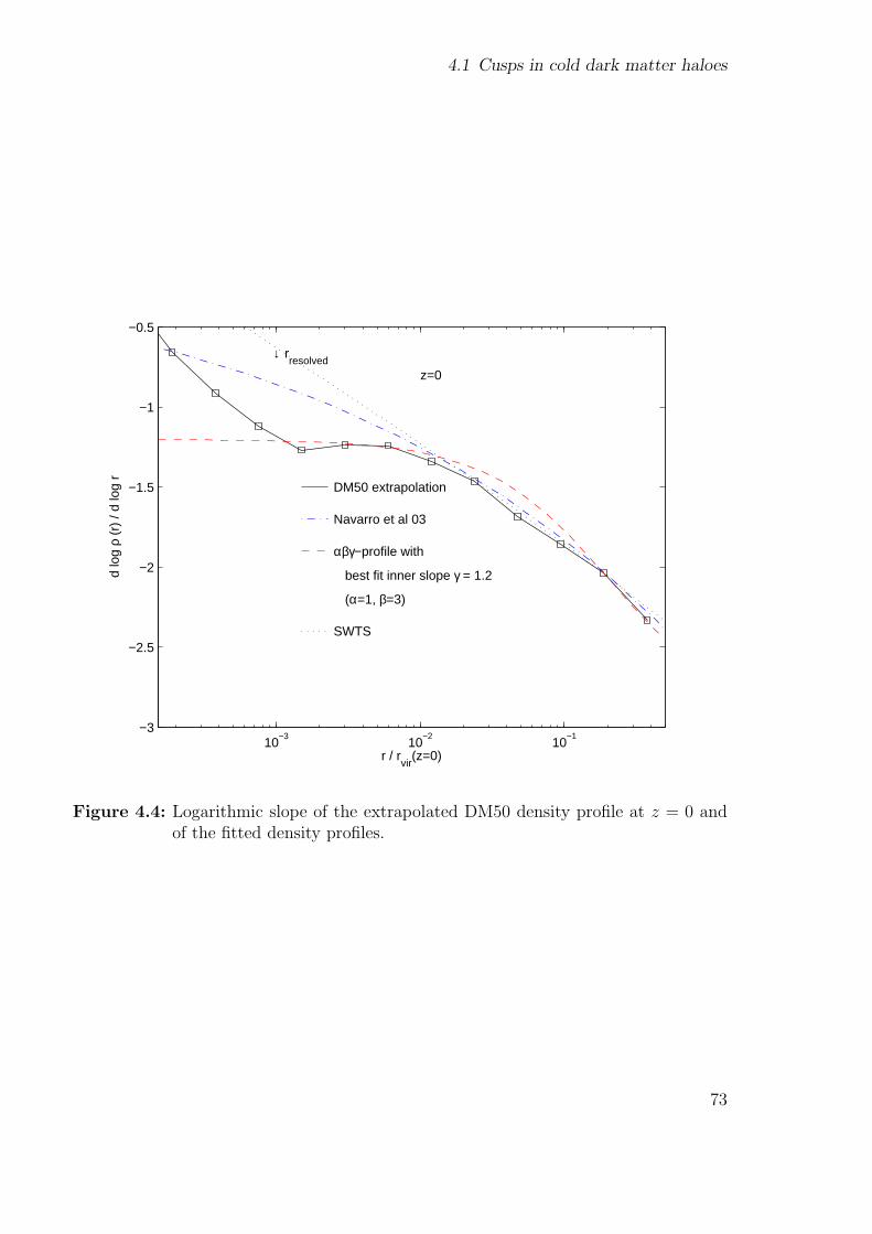
4.1 Cusps in cold dark matter haloes
10−3
10−2
10−1
−3
−2.5
−2
−1.5
−1
−0.5
r / rvir
(z=0)
d lo
g ρ
(r)
/ d lo
g r
z=0
DM50 extrapolation
Navarro et al 03
αβγ−profile with
best fit inner slope γ = 1.2
(α=1, β=3)
SWTS
↓ rresolved
Figure 4.4: Logarithmic slope of the extrapolated DM50 density profile at z = 0 andof the fitted density profiles.
73

Chapter 4 Applications
Figure 4.4 shows the slope of the extrapolated DM50 profile at z = 0 in comparisonwith the slopes of the best fits. It is evident that in the inner part the cuspy profile withγ = 1.2 describes the real density profile better.
4.2 Does the Fornax dwarf spheroidal have a centralcusp or core?2
4.2.1 Introduction
The Fornax dwarf spheroidal is a dark matter dominated satellite orbiting the MilkyWay. It has five globular clusters that are at a projected distance from the centre of1.60, 1.05, 0.43, 0.24 and 1.43 kpc [93] as well as further substructure at a projecteddistance of 0.67 kpc [25]. These star clusters move within a dense background of darkmatter and should therefore be affected by dynamical friction, causing them to loseenergy and spiral to the centre of the galaxy. We will show later that, if Fornax hasa cosmologically consistent density distribution of dark matter, the orbital decay time-scale of these objects from their current positions is approximately 5 Gyr. This is muchshorter than the age of the host galaxy, presenting us with the puzzle of why these fiveglobulars have not merged together at the centre forming a single nucleus [152, 153].
Several groups have studied the origin of nuclei in galaxies: e.g. Lotz et al. [91] carriedout Monte-Carlo simulations, which show that some, but not all, of the nuclei of dwarfelliptical galaxies could indeed have formed through coalescence of their globular clusters.Additionally they observed several dwarf elliptical galaxies and found out that withinthe inner few scale lengths, their sample appeared to be depleted of bright clusters. Ohand Lin [118] used numerical simulations to show that in dwarf galaxies with relativelyweak external tidal perturbations, dynamical friction can lead to significant orbital decayof globular clusters and the formation of compact nuclei within a Hubble time-scale.
Oh et al. [119] gave two possible models for the observed spatial distribution of Fornaxglobulars. One possibility they proposed is that the dark matter consists of massive blackholes which transfer energy to the globulars, preventing them from sinking to the centreof the galaxy. Another possibility they investigated was to postulate a strong tidalinteraction between the Milky Way and Fornax which also could inject energy into theirorbits and the central core of the dwarf spheroidals. This latter idea is probably ruledout due to the proper motion observations of Fornax [39] which suggest it is already atclosest approach on an extended orbit which never takes it close to the Milky Way.
Here we investigate another possibility for the lack of a nucleus in Fornax, namely thatthe central dark matter distribution has a very shallow cusp or core which dramaticallyincreases the dynamical friction sinking time-scale [70]. This would be inconsistent withdark haloes that form within the cold dark matter cosmology which have cusps steeperthan γ = −1 (ρ(r) ∝ r−γ) on all mass scales from 10−6 M¯ − 1015 M¯ [37, 40].
Controversial evidence for cored mass distributions in dwarf spiral galaxies has been
2Original publication: MNRAS, 368, 1073 (2006) [64]
74

4.2 Does the Fornax dwarf spheroidal have a central cusp or core?
debated for over a decade [107]. The inner structure of spheroidal galaxies is harderto determine, however Kleyna et al. [82] claimed that the second peak in the stellarnumber density in the nearby Ursa Minor dwarf spheroidal, is incompatible with cuspedcold dark matter haloes. With their observations they show that this substructure hasa cold kinematical signature and that its radial velocity with respect to its host galaxyis very small. Such a cold configuration could only survive intact if the stars orbitedwithin a cored mass distribution where the orbital frequencies are all identical (harmonicpotential) and phase mixing does not occur.
The stellar kinematical data for Fornax suggest that it is dark matter dominatedwith a mass to light ratio of order 20 within its optical extent. Due to the uncertaintyon the orbital anisotropy, the mass distribution can only be weakly constrained - thedata is consistent with either cusped or cored density distributions [90]. However thenormalisation (or mass within the central 1 kpc) is better constrained. In the inner∼ 1 kpc of a cored halo the mean density is approximately six times lower than in acusped halo. Furthermore the velocity distribution function of the background particlesis hotter than a cusped halo. These facts conspire to significantly increase the dynamicalfriction time-scale in a cored mass distribution.
We constructed cored and cuspy dark matter potentials and calculated orbital decayand sinking times using high resolution numerical simulations together with analyticcalculations [21]. The haloes were consistent with the kinematical data for Fornax. Wefollowed circular and eccentric orbits of single and multiple globular clusters. Althoughmany dynamical friction studies have been carried out before [19, 72, 165], we are notaware of any studies within constant density cores at the resolution used in this study,although a recent study explored the effects of sinking objects on various cusp structures[105].
4.2.2 Numerical methods
We carried out a series of self consistent simulations to examine the orbital behaviour ofmassive particles moving within a dark matter or stellar background. All the runs wereevolved with PKDGRAV (see section 1.3.5). For our simulations we used αβγ-modelsdescribed by equation (2.1) with α = 0.5 − 1.5, β = 3.0 and γ = 0.5 − 1.5, or coredhaloes with α = 0.5− 1.5, β = 3.0 and γ = 0.0.
In the former case we have ρ0 = 0.0058 M¯ pc−3 and rs = 2.4 kpc. This cuspy halohas a virial mass of 2.0 × 10⁹ M¯. The concentration parameter is c = 15 but ourresults would not change with a lower concentration, since in either case we are withinthe asymptotic cusp part of the density profile. We used the multi-mass technique: 105
particles for the innermost sphere with 100 pc radius, 105 particles for the shell between100 and 500 pc and 105 particles for the rest of the halo. The softening lengths of theparticles in these shells are 1, 10 and 100 pc respectively. The results were found not tobe sensitive to these values. The particle masses are 58 M¯, 569 M¯ and 3.2 ×10⁴ M¯.These models are stable in isolation but allow us to achieve very high resolution at thehalo centre where we wish to follow the dynamical friction.
For a small cored halo we have ρ0 = 0.10 M¯ pc−3 and rs = 0.91 kpc (n.b. the radius
75

Chapter 4 Applications
at which the slope of the density profile is shallower than -0.1 is approximately 200 pcwhich defines the constant density region in this model). This halo has a virial mass of2.0 × 109 M¯ and the concentration parameter is c = 40. Again, we use a three shellmodel that has 105 particles for the innermost sphere with 300 pc radius, 105 particlesfor the shell between 0.3 and 1.1 kpc and 3× 10⁵ particles for the rest of the halo. Thesoftening lengths of the particles in these shells are 3, 30 and 300 pc respectively. Theparticle masses are 89 M¯, 1640 M¯ and 7572 M¯. For a big cored dark matter halowe have basically the same parameters as for the halo with the small core, except forthe scale length rs = 2.2 kpc (here the constant density region is approximately 1 kpc),the virial mass Mvir = 3.0× 10¹⁰ M¯ and the particle masses, which are in this case 106M¯, 3625 M¯ and 1.2× 10⁵ M¯.
4.2.3 Results
Single globular clusters
From the Chandrasekhar dynamical friction formula [15, 21], we can derive an expressionfor the radial sinking velocity of the globular cluster with mass MGC at radius r
dr
dt= −4π ln Λ(r)ρ(r)G2MGCr
v2c (r)d[rvc(r)]/dr
[erf
(vc(r)√2σ(r)
)− 2vc(r)√
2πσ(r)exp
(− v2
c (r)
2σ2(r)
)](4.3)
where G is Newtons constant of gravity, vc(r) is the local circular velocity, σ(r) is thelocal velocity dispersion, ρ(r) is the local density and ln Λ(r) = bmaxσ
2(r)/GMGC is theCoulomb logarithm.
In figure 4.5, we plot the numerical fits from equation (4.3) for different haloes andinitial radii for the orbital decay of a single globular cluster where bmax was used as afree fitting parameter. The globular clusters are modelled as single particles of massMGC = 2 × 10⁵ M¯ with a softening of 10 pc. We do not expect our conclusions tochange if we used a particle model for each globular since they are stable against tidaldisruption within Fornax. We start the globulars outside the core, mostly on circularorbits and let them orbit, expecting them to spiral in to the centre of their respectivehost haloes due to dynamical friction. For the cuspy halo the analytic calculation agreesvery well with the numerical simulation. Haloes with a core give a poorer agreement.After an initial sinking rate that agrees well with the analytic expectation, the globularssink faster as they approach twice the core radius, and then stop sinking at the coreradius. The stalling results are apparent in both of the cored halo simulations (small coreand big core). We note, however, that it is not trivially due to the fact that the globularis of comparable mass to that enclosed by its orbit; the radius at which M(r) = MGC
is approximately three times smaller than the core radius (see figure 4.7). We concludethat the presence of a central density core leads to a stopping of the infall of the clustersat approximately the core radius.
76
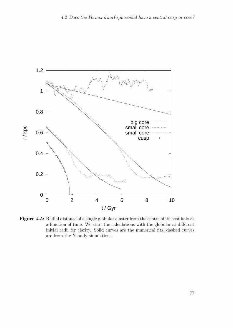
4.2 Does the Fornax dwarf spheroidal have a central cusp or core?
0
0.2
0.4
0.6
0.8
1
1.2
0 2 4 6 8 10
r / k
pc
t / Gyr
big coresmall coresmall core
cusp
Figure 4.5: Radial distance of a single globular cluster from the centre of its host halo asa function of time. We start the calculations with the globular at differentinitial radii for clarity. Solid curves are the numerical fits, dashed curvesare from the N-body simulations.
77

Chapter 4 Applications
Multiple globular clusters
We re-ran these simulations using five globulars to study the effect of having multiplesinking objects. Perhaps interactions between the globulars themselves may preventthem from sinking to the central cusp and merging. We distribute the globulars ran-domly, what position and plane of the orbit concerns, with distances to the centrebetween 0.2 and 1.2 kpc. The clusters are again placed on circular orbits around thecentre of their host halo.
Interestingly, the clusters do not prevent one another from falling to the centre, butinstead create an interesting prediction. Figure 4.6 shows the infall as a function of timefor the five globulars in the cuspy dark matter halo. Notice that all of the clusters fallto the centre within 5 Gyr. However, clusters which start out at very similar radii arriveapproximately 1 Gyr apart. At any given time, even for very similar initial conditions,the clusters occupy a range of radii.
By contrast, for the case with a central dark matter core (see figure 4.7), although theglobulars still arrive at different times due to interactions, they stall at the core radius;they do not sink to the centre even within 18 Gyr. Thus, if Fornax does have a centralconstant density core we should expect the clusters to stall at some minimum radius.No globular cluster could possibly get any closer to the centre of the halo than the coreradius. The lower limit of the core size is constrained by the smallest observed projectedcluster distances to be 0.24 kpc.
78

4.2 Does the Fornax dwarf spheroidal have a central cusp or core?
0
0.1
0.2
0.3
0.4
0.5
0.6
0.7
0.8
0 0.5 1 1.5 2 2.5 3 3.5 4 4.5 5
r / k
pc
t / Gyr
Figure 4.6: Radial distance of the five globular clusters from the centre of their hosthalo as function of time, as they orbit within a cuspy halo. The arrowindicates the radius at which MGC = M(r).
79

Chapter 4 Applications
0
0.2
0.4
0.6
0.8
1
1.2
0 2 4 6 8 10 12 14 16 18
r / k
pc
t / Gyr
Figure 4.7: Radial distance of the five globular clusters from the centre of their hosthalo as function of time, as they orbit within a cored halo. The upper arrowindicates the size of the core and the lower arrow indicates the radius atwhich MGC = M(r).
80

Chapter 5
Summary and perspective
Summary
Resolving the fast dynamics in the centres of galaxies requires reconsidering the time-stepping method that is used to integrate the equations of motion. The standard time-stepping criterion used by most of the numerical codes so far is based on the accelerationof a particle. Unfortunately, with this method, one is only able to resolve regions of darkmatter haloes down to approximately one per cent of the virial radius. Below that scale,the standard criterion fails completely to follow the dynamics of the simulations withthe standard parametes normally used. It even gives an incorrect, in fact unphysicalselection of time-steps in regions where the local density profile is flat, e.g. time-stepsstay constant or even increase for particles closer to the centre due to the functionalform of the acceleration with radius. This can only be adjusted by choosing a smallprefactor ηS but as a consequence, the simulations become very slow.
The new time-step criterion determines the true dynamical time of each particle andsets this as the time-step. In the case of hard gravitational scattering events, an ec-centricity correction for the integration method is used in order to follow the orbitsprecisely. With this method, we are able to resolve the dynamics at the centres of denseself-gravitating systems. By choosing an appropriate softening length for the particles,we can even resolve high eccentricity orbits during gravitational scattering events allow-ing the method to handle collisionless as well as collisional dynamics simultaneously.
In addition to correctly treating the physics the new method results in a substan-tial speed-up compared to traditional approaches since the dynamical time-step crite-rion is much more adaptive with radius, preventing particles from being integrated onoverly conservative small time-steps. Also, the method does not directly depend onnon-physical parameters like the softening length.
In order to resolve parsec scales in dark matter haloes, one would need billions ofparticles for a single halo model, a requirement that is still prohibitive with existingcomputational resources. The developed of a multi-mass technique for generating highresolution dark matter haloes allows to resolve the scales where the dynamics of, e.g.,a super-massive black hole binary becomes dominant and interacts significantly withits surroundings. Such studies were so far only possible for restricted cases and lowresolution.
The multi-mass technique was already used in several applications that needed high
81

Chapter 5 Summary and perspective
spatial resolution. In a test case for the multi-mass technique, we confirm earlier findingsand predictions that core-core mergers lead to a cored merger remnant while cups-cusp mergers lead to a cuspy merger remnant with high resolution multi-mass N-bodysimulations. In cusp-core merges, the merger remnant has a final profile correspondingto the steepest progenitor. In a cosmological structure formation simulation, the multi-mass technique was used to resolve the dark matter halo of a galaxy cluster down toone per mill of the virial radius which corresponds to an effective resolution of onebillion particles. We found that the central profile still follows a power law with slope ofapproximately γ = −1.2, where ρ(r) ∝ r−γ. A further application tested a model thatcan explain the presence of the five globular clusters at approximately 1 kpc distanceform the centre of the Fornax dwarf spheroidal galaxy.
Perspective
These new techniques enable the exploration of an unknown area of N-body simulations.Therefore, the main goals for the future are to apply these techniques in the primaryapplication it was designed for: in mergers of galaxies with super-massive black holesand study the dynamical effects involved in this process.
Once the black hole binary is formed through the merger of the galaxies it may alsohave an influence on the density profile of the surrounding dark matter halo. The blackhole binary may transfer energy to the surrounding particles in the high-density centralregion through the slingshot-effect, which leads to a shallower central density profile ofthe dark matter. The question of the central density is very important, since one of theobservational consequences of this is an observable flux of gamma-rays from the innerfew parsecs of the halo due to self-annihilation of dark matter [63]. The flux is verysensitive to the central dark matter density. Establishing the stability of the centraldark matter cusp to dynamical perturbations is therefore of paramount importance toplanning and interpreting the data that will be soon provided by major facilities, suchas the 17 m MAGIC1 telescope, which are designed to measure such a signal. Therewere previous studies of this problem [101, 104], which were limited in resolution. Weintend to address this issue by performing simulations in a self-consistent way, with theneeded resolution that includes the large-scale dynamics from the dark matter halo andthe small-scale collisional physics in the centre of the galaxies.
Yu and Tremaine [172] postulated that a possible mechanism for the origin of hyper-velocity stars (i.e. stars moving with incredible high velocity such that they possiblywill escape the galaxy) is the gravitational scattering by massive binaries (black hole orstars or a combination of the two) in the centre of galaxies. Studying the characteristicsof these hyper-velocity stars is important to predict the expected parameter space forfuture observational programs that would allow detecting these fast stars systematically.We plan to study this in a self-consistent way and examine the dependence of the orbitsof the ejected stars on the triaxiality of the halo.
1magic.mppmu.mpg.de
82

In the hierarchical paradigm, successive mergers between spheroids that host blackholes may lead to the accelerated formation of super-massive black holes at the centres ofgalaxies [75, 94]. This process has interesting and potentially observable consequences,including a large population of black holes orbiting within and through the galaxy thatejected them through 3-body encounters. Using high resolution N-body simulations ofstructure formation in a cold dark matter universe, we can test two distinct scenariosfor the formation of super-massive black holes: (i) A final central black hole may formdue to the hierarchical merger of thousands of small dark matter haloes. Through someprocess, each of the progenitor haloes may contain a small black hole. As the mergerstake place the black holes spiral inwards in the cuspy dark matter potentials, eventuallymerging together through energy loss from gravitational radiation. (ii) Black holes formin a population of globular clusters that form within the rare dark matter mini-haloes ata redshift z = 10− 20. These undergo a rapid merging process to create a single centralsuper-massive black hole. In such a calculation it is important to be able to closelyfollow the dynamical interactions between the black holes, which is why it is importantto employ the new time-stepping algorithm and study these interactions within a self-consistently modelled cosmological context. Our aim is to investigate whether it ispossible to form a single central super-massive black hole, and to study the spatial andkinematical distribution of ejected black holes.
A possible drawback might be the enormous amount of computer run time that isneeded for such simulations. Possible solutions like introducing hierarchies of trees wheresome parts of the simulations are frozen while only particles in very-active regions of thesimulation are evolved or loosening the strict geometrical definition of the dynamicaltime are already under development.
But for future high resolution N-body simulations, the only efficient time-steppingscheme has to be based on the true dynamical time since it shows the optimum scalingwith the number of particles used and always gives a physically correct time-step.
83

Chapter 5 Summary and perspective
84

Appendix
85


Appendix A
Hamiltonian formalism
For a physical system that is described by the state z = (q ,p), where q is the coordinateand p the conjugate momentum vector, and this system is evolved under a HamiltonianH, we can write the formal time evolution (Hamilton equations) as [15, 132, 171]
dz
dt= z = z , H (A.1)
where , denote the Poisson brackets defined by
g, h ≡f∑i
(∂g
∂qi
∂h
∂pi
− ∂g
∂pi
∂h
∂qi
). (A.2)
We can define the operator H by
Hz ≡ z , H (A.3)
and write down a formal solution to the time evolution
z (t) = etHz 0 . (A.4)
In computer simulations, the system is evolved by using a specific scheme in order toupdate positions and velocities. In PKDGRAV, the following leapfrog scheme is used:during a time-step ∆T , first the velocities are updated (kick mode) with a time step of∆T/2 then the new positions are calculated (drift mode) using the new velocities witha time-step of ∆T and finally the velocities are updated to the final values at ∆T withagain a half-step of ∆T/2 but with the acceleration calculated from the new positions.This scheme can be written as
v(t + ∆T/2) = v(t) + ∆T/2 a(t) (A.5)
x (t + ∆T ) = x (t) + ∆T v(t + ∆T/2) (A.6)
v(t + ∆T ) = v(t + ∆T/2) + ∆T/2 a(t + ∆T ) (A.7)
and is therefore called the kick-drift-kick mode. We can write it in the operator formalismas
z (∆T ) = e∆T2
HKe∆THDe∆T2
HKz 0 (A.8)
87

Appendix A Hamiltonian formalism
where we have split the true Hamiltonian into a drift and a kick part
H = HD + HK . (A.9)
By using the Baker-Campbell-Hausdorff series, where we can calculate the higher orderterms by an elegant method developed by Reinsch [130], we can write the approximateoperator HA under which the system is evolved
z (∆T ) = e∆T2
HKe∆THDe∆T2
HKz 0 = e∆THAz 0 (A.10)
by
HA = H0 + ∆T 2H2 + ∆T 4H4 + O(∆T 6) (A.11)
where
H0 = HD + HK = H (A.12)
H2 =1
12
[[HK, HD
], HD
]− 1
24
[[HD, HK
], HK
](A.13)
H4 =7
5760
[[[[HD, HK
], HK
], HK
], HK
](A.14)
7
1440
[[[[HD, HK
], HD
], HK
], HK
]
− 1
360
[[[HD, HK
], HK
],[HD, HK
]]
− 1
180
[[[[HK, HD
], HK
], HD
], HD
]
− 1
360
[[[HK, HD
], HD
],[HK, HD
]]
− 1
720
[[[[HK, HD
], HD
], HD
], HD
].
Here, [, ] denote the commutator brackets defined by
[A,B] = AB −BA (A.15)
for non-commutative operators A and B. By using the definitions of the operators andthe Jacobi identity for Poisson brackets
A,B, C+ B, C, A+ C, A, B = 0 , (A.16)
we can calculate the approximate Hamiltonian
HA = H0 + ∆T 2H2 + ∆T 4H4 + O(∆T 6) (A.17)
88

where
H0 = HD + HK = H (A.18)
H2 =1
12HK, HD , HD − 1
24HD, HK , HK (A.19)
H4 =7
5760HD, HK , HK , HK , HK (A.20)
7
1440HD, HK , HD , HK , HK
− 1
360HD, HK , HK , HD, HK
− 1
180HK, HD , HK , HD , HD
− 1
360HK, HD , HD , HK, HD
− 1
720HK, HD , HD , HD , HD .
Note that the replacement of the commutator brackets by the Poisson brackets is nottrivial. The term H4 is not used in our method. However, since H4 is not explicitlygiven in the recent literature we present it here for completeness.
89

Appendix A Hamiltonian formalism
90

Appendix B
Further projects
This chapter is a short summary of further projects in which the author of this thesiswas involved as a co-author. These projects are not related to the main developmentsof the thesis.
B.1 A universal velocity distribution of relaxedcollisionless structures1
B.1.1 Introduction
The last few years have shown remarkable progress in the understanding of pure darkmatter structures. This has been provided initially by numerical simulations which haveobserved general trends in the behaviour of the radial density profile of equilibrateddark matter structures from cosmological simulations, which roughly follow an NFWprofile [110, 112, 116, see also equation (2.1)] with central density profile slope γ =1.0. General trends in the radial dependence of the velocity anisotropy has also beensuggested [20, 24]. More recently have more complex relations been identified, whicheven hold for systems which do not follow the most simple radial behaviour in density.These relations are first that the phase-space density, ρ/σ3, is a power-law in radius[150], and second that there is a linear relationship between the density slope and theanisotropy [67].
All of these are integrated quantities, and still very little is known about the underlyingvelocity distribution function of real collisionless systems. We initiated such a study byperforming a set of different simulations of purely collisionless systems.
B.1.2 Numerical methods and results
The first controlled simulation were head-on collision between two equal spherical NFWstructures. We created three different initial conditions. The first model had an isotropicvelocity structure. For the other two models we kept the kinetic energy of a particlefrom the isotropic model fix but rotated the velocity vector so that it pointed to thecentre (radial initial conditions) or were tangential (tangential initial conditions). For
1Original publication: JCAP, 1, 14 (2006) [69]
91

Appendix B Further projects
the construction of the initial structures, we used the method as described in Kazantzidiset al. [80]. We created an initial NFW structure containing one million particles. Theparameters were chosen corresponding to a total mass of 1012 M¯ (concentration ofc = 10), and half of the particles were within 160 kpc.
We placed two such structures with equal velocity structure very far apart with 2000kpc between the centres, which is well beyond the virial radius. Using a softening of 0.2kpc, we let these two structures collide head-on with an initial relative velocity of 100km s−1 towards each. After several crossings the resulting blob relaxed into a prolatestructure. We run all simulations until there was no further time variation in the radialdependence of the anisotropy and density. We checked that there is no (local) rotation.We run this simulation for 150 Gyr, which meant that a very large part of the resultingstructure is fully equilibrated.
We now took the resulting structure (now containing two million particles, in a prolateshape) and collided two copies together, again with their centres separated by 2000 kpc,and with initial relative velocity of 100 km s−1. We used softening of 1 kpc. The resultingstructure is even more prolate when observed in density contours, and we evolved thisfor another 150 Gyr. All simulations were carried out using PKDGRAV (see section1.3.5).
In order to analyse the resulting structure we divided it into bins in potential energy,linearly distributed from the softening length to beyond the region which is fully equi-librated. For the analysis and figures presented here, we always only included a regionoutside three times the softening. We centred the structure on the centre of potential(using potential as weight-function instead of mass as done for centre of mass). Mostother analyses are centring on either the centre of mass, or on the most bound particle,but the difference is very small. We calculated the local density for each particle fromits nearest 32 neighbours, and we averaged the density for all the particles in the poten-tial bin. Similarly, each particle had a radius from the centre of potential, and we canaveraged this over all the particles in the potential bin. The resulting density profile,〈ρ〉 as a function of 〈r〉, was very similar to an NFW profile.
For each bin we can also defined the radial derivative of the density (the density slope)
α ≡ d ln〈ρ〉d ln〈r〉 , (B.1)
and we can extracted the radial velocity distribution function for each potential bin. Wepresent the radial velocity distribution function for bins with α ≈ −2.6,−2 and −1.1 infigure B.1. The red (open) stars are from a bin in the region with shallow density slope(α ≈ −1.1), the green (open) squares are from an intermediate bin (slope close to −2),and the blue (filled) triangles are from a bin in the outer region (slope close to −2.6).There seems to be a clear trend, namely that the velocity distribution function from binsin the inner region have longer high energy tails than velocity distribution functions frombins in the outer region. The high energy tail of the radial velocity distribution function
92

B.1 A universal velocity distribution of relaxed collisionless structures
Figure B.1: The radial velocity distribution function for three potential bins in thesimulation of repeated head-on collisions between NFW structures withvery different initial conditions: isotropic (left), radial (middle) and tan-gential (right) velocity distributions. The potential bins are chosen neardensity slope of α ≈ −1.1 (open red stars), α ≈ −2 (open green squares)and α ≈ −2.6 (filled blue triangles). The thin (solid) lines are of theshape given by equation (B.2), using q’s of 0.75, 0.81 and 1.08 (isotropic);q = 0.79, 0.91 and 1.05 (radial) and q = 0.75, 0.89 and 1.045 (tangential).
is well approximated by the shape given by
fr(v) =
(1− (1− q)
(v
κrad σrad
)2) q
1−q
, (B.2)
where q and κrad are free parameters. This is of the Tsallis form [154] and depends onthe entropic index q. For q = 1, equation B.2 reduces to the Gaussian shape f(v) ∝exp(−(v/v0)
2). This functional form is chosen partly for simplicity (and because itincludes the classical exponential) and partly because some simple structures are knowto have velocity distribution functions of exactly this form [68, 124]. In particulardo we see that the resulting velocity distribution functions do not have the shape ofGaussians with a cut-off at the escape velocity. It is clear from figure B.1 above, thatthe simple shape of equation (B.2) provides a reasonable fit to the tails of the radialvelocity distribution functions.
The two-dimensional generalisation of the form (B.2) is given by
ft(v) = v
(1− (1− q)
(v
κtan σtan
)2) q
1−q
. (B.3)
The tangential velocity distributions ft(v) can be fitted by two such shapes: one in thesmall velocity region, and another in the high velocity region. It was argued in Hansenand Moore [67] that the tangential velocity distribution functions could have the shapeof equation (B.3) with q = 5/3, and the small velocity region is very well fit with exactlythis shape for all the bins in potential.
93

Appendix B Further projects
Figure B.2: The tangential velocity distribution functions from all the simulations de-scribed. The black (solid) line has two parts (separated at vtan = 1.6 σtan),each fitted with the shape given in equation (B.3), where the low energypart uses q = 5/3, and the outer region (high energy part) has a free q.Left: using a potential bin near the density slope of α = −1.1, and theblack (solid) line uses q = 0.9 in the high energy part. Middle: α = −2,q = 0.86. Right: α = −2.6, q = 0.76.
We pick the position vtan = 1.6 σtan as the transition velocity for all figures, and fitthe high energy region with the shape of equation (B.3), but with q as a free parameter.The combined fit is shown as black (solid) lines in figure B.2.
But not only the velocity distribution functions from the resulting remnants of thesecontrolled head-on collisions can be described by the functional form given by (B.2)respectively (B.3). We also examined haloes from cosmological structure formation runsor remnants of radial infall simulations and their velocity distribution functions have thesame shape as already described.
Hence, we have identified a universality of the velocity distribution function of equi-librated structures of collisionless, self-gravitating systems through a set of numericalexperiments. The radial and tangential velocity distribution functions are universal inthe sense that they depend only on the dispersion (radial or tangential) and the localslope of the density. There is a general trend, namely that a steeper density slope impliessmall q. The actual shape of the velocity distribution functions is not understood yet.These numerical results may hopefully inspire further theoretical understanding of thevelocity distribution function of collisionless particles.
94

B.2 Globular clusters, satellite galaxies and stellar haloes from early dark matter peaks
B.2 Globular clusters, satellite galaxies and stellarhaloes from early dark matter peaks2
B.2.1 Introduction
The Milky Way is a typical bright spiral galaxy. Its disk of stars and gas is surroundedby an extended halo of old stars, globular star clusters and a few dark matter dominatedold satellite galaxies. For the past 30 years two competing scenarios for the origin ofgalaxies and their stellar components have driven much observational and theoreticalresearch. Eggen et al. [43] proposed a monolithic collapse of the Galaxy whilst Searleand Zinn [136] advocated accretion of numerous proto-galactic fragments.
Enormous progress has been made in understanding the structure and origin of theMilky Way, as well as defining a standard cosmological model for structure formationthat provides us with a framework within which to understand our origins [51, 122].Hierarchical growth of galaxies is a key expectation within a universe whose mass isdominated by a dark and nearly cold particle, yet evidence for an evolving hierarchyof merging events can be hard to find, since much of this activity took place over tenbillion years ago. The origin of the luminous Galaxy depends on the complex assemblyof its approximately 1012 M¯ dark matter halo that extends beyond 200 kpc, and onhow stars form within the first dark matter structures massive enough to cool gas tohigh densities [166].
The Galactic halo contains about 100 old metal poor globular clusters (i.e. Forbeset al. [50]) each containing up to 106 stars. Their spatial distribution falls off as r−3.5 atlarge radii and half the globulars lie within 5 kpc from the centre of the Galaxy [147].There is no evidence for dark matter within the globular clusters today [108, 123]. Theold stellar halo population has a similar spatial distribution and a total luminosity of108−109 L¯3 [76, 95]. The stellar populations, ages and metallicities of these componentsare very similar [51].
Also orbiting the Galaxy are several tiny spheroidal satellite galaxies, each containingan old population of stars, some showing evidence for more recent star-formation indi-cating that they can hold on to gas for a Hubble time [55, 65]. Half of the dwarf satelliteslie within 85 kpc, have luminosities in the range 106 − 108 L¯ and are surrounded bydark matter haloes at least 50-200 times as massive as their baryonic components [98].Cold dark matter models have had a notoriously hard time at reconciling the observedlow number of satellites with the predicted steep mass function of dark matter haloes[79, 83, 111].
We wish to explore the hypothesis that cold dark matter dominates structure forma-tion, the haloes of galaxies and clusters are assembled via the hierarchical merging andaccretion of smaller progenitors [88]. This process violently causes structures to cometo a new equilibrium by redistributing energy among the collisionless mass components.Early stars formed in these progenitors behave as a collisionless system just like the dark
2Original publication: MNRAS, 368, 563 (2006) [115]3L¯ stands for the luminosity (radiated enregy per unit time) of the Sun. L¯ = 3.826× 1026 J s−1.
95

Appendix B Further projects
matter particles in their host haloes, and they undergo the same dynamical processesduring subsequent mergers and the buildup of larger systems like massive galaxies orclusters.
In a recent study, Diemand et al. [36] used cosmological N-body simulations to explorethe distribution and kinematics in present-day cold dark matter haloes of dark matterparticles that originally belonged to rare peaks in the matter density field. These proper-ties are particularly relevant for the baryonic tracers of early cold dark matter structures,for example the old stellar halo which may have originated from the early disruption ofnumerous dwarf proto-galaxies [17], the old halo globular clusters and also giant ellipti-cals [56].
Since rare, early haloes are strongly biased towards overdense regions [137], i.e. to-wards the centres of larger scale fluctuations that have not collapsed yet, we might expectthat the contribution at z = 0 from the earliest branches of the merger tree is muchmore centrally concentrated than the overall halo. Indeed, a non-linear peaks biasinghas been discussed by previous authors [109, 110, 167]. Diemand et al. [36] showedthat the present-day distribution and kinematics of material depends primarily on therareness of the peaks of the primordial density fluctuation field that the selected matteroriginally belonged to, i.e. when selecting rare density peaks above νσ(M, z) (whereσ(M, z) is the linear theory rms density fluctuations smoothed with a top-hat filter ofmass M at redshift z), their properties today depend on ν and not on the specific valuesof selection redshift z and minimal mass M .
B.2.2 The first stellar systems
We propose that ordinary Population II stars and globular clusters first appeared insignificant numbers at redshift z > 12, as the gas within protogalactic haloes with virialtemperatures above 104 K (corresponding to masses comparable to those of present-daydwarf spheroidals) cooled rapidly due to atomic processes and fragmented.
It is this second generation of subgalactic stellar systems, aided perhaps by an earliergeneration of metal-free (Population III) stars and by their remnant black holes, whichgenerated enough ultraviolet radiation to reheat and reionize most of the hydrogen inthe Universe by a redshift z = 12, thus preventing further accretion of gas into theshallow potential wells that collapsed later. The impact of a high redshift ultravioletradiation background on structure formation has been invoked by several authors [7, 10,17, 66, 109, 155] to explain the flattening of the faint end of the luminosity functionand the missing satellites problem within our Local Group. Here we use high resolutionnumerical simulations that follow the full non-linear hierarchical growth of galaxy masshaloes to explore the consequences and predictions of this scenario.
Dark matter structures will collapse at different times, depending on their mass, butalso on the underlying larger scale fluctuations. At any epoch, the distribution of massesof collapsed haloes is a steep power law towards low masses with n(m) ∝ m−2. To makequantitative predictions we calculate the non-linear evolution of the matter distributionwithin a large region of a ΛCDM universe. The entire well resolved region is about 10comoving Mpc across and contains 61 million dark matter particles of mass 5.85×10⁵ M¯
96

B.2 Globular clusters, satellite galaxies and stellar haloes from early dark matter peaks
Figure B.3: The high redshift and present day mass distribution in a region that formsa single galaxy in a hierarchical cold dark matter universe.
97

Appendix B Further projects
and force resolution of 0.27 kpc. This region is embedded within a larger 90 Mpc cubethat is simulated at lower resolution such that the large scale tidal field is represented.Figure B.3 shows the high-redshift and present-day mass distribution of a single galaxymass halo taken from this large volume. The upper panel shows the density distributionat a redshift z = 12 from a region that will form a single galaxy at z = 0 (lowerpanel). The rare peaks collapsing at high redshift that have had sufficient time to coolgas and form stars, can be identified, followed and traced to the present day. Becausesmall fluctuations are embedded within a globally larger perturbation, the small rarerpeaks that collapse first are closer to the centre of the final potential and they preservetheir locality in the present day galaxy. The strong correlation between initial andfinal position results in a system where the oldest and rarest peaks are spatially moreconcentrated than less rare peaks. The present day spatial clustering of the materialthat was in collapsed structures at a higher redshift only depends on the rarity of thesepeaks [36].
Our simulation contains several well resolved galactic mass haloes which we use totrace the evolution of progenitor haloes that collapse at different epochs. The first metalfree Population III stars form within minihaloes already collapsed by z > 25, where gascan cool via roto-vibrational levels of H2 and contract. Their evolution is rapid and localmetal enrichment occurs from stellar evolution. Metal-poor Population II stars form inlarge numbers in haloes above MH ≈ 108 [(1+z)/10]−3/2 M¯ (virial temperature 104 K),where gas can cool efficiently and fragment via excitation of hydrogen Lyα. At z > 12,these correspond to > 2.5 σ peaks of the initial Gaussian overdensity field: most of thismaterial ends up within the inner few kpc of the Galaxy. Within the approximately 1Mpc turn-around region, a few hundred such protogalaxies are assembling their stellarsystems [85]. Typically 95% of these first structures merge together within a time-scaleof a few Gyr, creating the inner Galactic dark matter halo and its associated old stellarpopulation.
With an efficiency of turning baryons into stars and globular clusters of the orderf∗ = 10% we successfully reproduce the total luminosity of the old halo population andthe old dwarf spheroidal satellites. The fraction of baryons in dark matter haloes abovethe atomic cooling mass at redshift z = 12 exceeds fc = 1%. A normal stellar populationwith a Salpeter-type initial mass function emits about 4000 hydrogen-ionizing photonsper stellar baryon. A star formation efficiency of 10% therefore implies the emission of4000×f∗×fc ∼ a few Lyman-continuum photons per baryon in the Universe. This maybe enough to photoionize and drive to a higher adiabat vast portions of the intergalacticmedium, thereby quenching gas accretion and star formation in nearby low-mass haloes.
B.2.3 Connection to globular clusters and halo stars
The globular clusters that were once within the merging proto-galaxies are so dense thatthey survive intact and will orbit freely within the Galaxy. The surviving proto-galaxiesmay be the precursors of the old satellite galaxies, some of which host old globularclusters such as Fornax, whose morphology and stellar populations are determined byongoing gravitational and hydrodynamical interactions with the Milky Way [100].
98

B.2 Globular clusters, satellite galaxies and stellar haloes from early dark matter peaks
10−2
10−1
100
10−2
10−1
100
101
102
103
104
105
106
r/rvir
ρ(r)
/ ρ cr
it.
all
1σ
2σ
2.5σ
3σ3.5σ
stellar halo ~ r−3.5
globular clustersdwarf galaxies
Figure B.4: The radial distribution of old stellar systems compared with rare peakswithin a z = 0 ΛCDM galaxy. The thick blue curve is the total massdistribution today. The labeled green curves show the present day dis-tribution of material that collapsed into 1, 2, 2.5, 3 and 3.5σ peaks at aredshift z = 12. The circles show the observed spatial distribution ofthe Milky Way’s old metal poor globular cluster system. The dashed lineindicates a power law ρ(r) ∝ r−3.5 which represents the old halo stellarpopulation. The squares show the radial distribution of surviving 2.5σpeaks which are slightly more extended than the overall NFW-like massdistribution, in good agreement with the observed spatial distribution ofthe Milky Way’s satellites.
99

Appendix B Further projects
Recent studies have attempted to address the origin of the spatial distribution ofglobular clusters [120, 121]. Most compelling for this model and one of the key resultsin this paper, is that we naturally reproduce the spatial clustering of each of these oldcomponents of the galaxy. The radial distribution of material that formed from > 2.5σpeaks at z > 12 now falls off as ρ(r) ∝ r−3.5 within the Galactic halo - just as theobserved old halo stars and metal poor globular clusters (see figure B.4). Cosmologicalhydrodynamical simulations are also begining to attain the resolution to resolve theformation of the old stellar haloes of galaxies [3]. Because of the steep fall off withradius, we note that we do not expect to find any isolated globular clusters beyond thevirial radius of a galaxy.
These first collapsing structures infall radially along filaments and end up significantlymore flattened than the mean mass distribution. They also have colder velocity distribu-tions and their orbits are isotropic in the inner halo and increasingly radially anisotropicin the outer part. Material from these rare peaks has βstd = 1 − 1
2(σ2
tan/σ2rad) ≈ 0.45
at our position in the Milky Way, in remarkable agreement with the recently measuredanisotropy and velocity dispersion of halo stars [9, 22, 151]. Diemand et al. [36] showthat the radial distribution of rarer peaks is even more highly biased - thus the oldestpopulation III stars and their remnant black holes are found mainly within the innerkpc of the Galaxy, falling off with radius steeper than r−4.
The observational evidence for tidal stellar streams from globular clusters suggeststhat they are not embedded within extended dark matter structures today [108]. Thisdoes not preclude the possibility that the globular clusters formed deep within the cen-tral region of 108 M¯ dark matter haloes which have since merged together. (Massivesubstructure within the inner ∼ 0.2 rvir of galactic mass haloes is tidally disrupted [61].)This is what we expect within our model which would leave the observed globulars freelyorbiting without any trace of the original dark matter component. However, it is pos-sible that the most distance halo globulars may still reside within their original darkmatter halo. If the globular cluster is located at the centre of the cold dark matter cusp,then observations of their stellar kinematics may reveal rising dispersion profiles. If theglobular cluster is orbiting within a cold dark matter mini-halo then we would expectto see symmetric tidal streams orbiting within the potential of the cold dark mattersubstructure halo rather than being stripped by the Galaxy.
B.2.4 Connection to satellite galaxies and the missing satellitesproblem
The remaining ∼ 5% of the proto-galaxies form sufficiently far away from the mayhemthat they fall into the assembling galaxy late (z ≈ 1− 2, about one Gyr after the forma-tion of the inner Galaxy at z ≈ 5). This leaves time to enhance their α/Fe element ratiosfrom Type II supernovae [127, 169, 170]. Recent studies including chemical modeling ofthis process support this scenario [49, 131].
The proto-galaxies highlighted with boxes in Figure B.3 are those few systems thatsurvive until the present epoch - they all form on the outskirts of the collapsing region,
100

B.2 Globular clusters, satellite galaxies and stellar haloes from early dark matter peaks
ending up tracing the total mass distribution as is also observed within the Milky Way’sand M31’s satellite systems. Each of our four high resolution galaxies contains about tenof these surviving proto-galaxies which have a radial distribution that is slightly shallowerthan that of the total mass distribution (see figure B.4) but more concentrated than thedistribution of all surviving (or z = 0 mass selected) subhaloes. This is consistent withthe spatial distribution of surviving satellites in the Milky Way and in other nearbygalaxies in the 2dF [133, 158] and DEEP2 samples [23] and with galaxy groups likeNGC5044 [46].
The total number of dark matter substructures in the Local Group is over an order ofmagnitude larger than the observations. Reionisation and photo-evaporation must playa crucial role in suppressing star formation in less rare peaks, thus keeping most of thelow mass haloes that collapse later devoid of baryons. The surviving population of rarepeaks had slightly higher masses just before accretion, tidal stripping inside the Galaxyhalo then reduced their masses and they match the observations at z = 0.
Likewise to the radial distribution, the kinematics of the surviving visible satellitegalaxies resembles closely the one of the dark matter while the same properties for all thesurviving subhaloes differ. In the inner part our model satellite galaxies are hotter thanthe dark matter background, especially in the tangential component. This is consistentwith the observed radial velocities of Milky Way satellites. For the inner satellites alsothe tangential motions are know (with large uncertainties however) [98, 168] and just asin our simple model they are larger than the typical tangential velocities of dark matterparticles in the inner halo.
The total (mostly dark) surviving subhalo population is more extended and hotterthan the dark matter while the distribution of orbits is similar [33]. Subhaloes tendto avoid the inner halo and those who lie near the centre at z = 0 move faster (bothin the tangential and radial directions) than the dark matter particles, i.e. these innersubhaloes have large orbital energies and spend most of their time further away fromthe centre (see also Diemand et al. [33]).
101

Appendix B Further projects
102

Bibliography
[1] S. J. Aarseth. Gravitational N-Body Simulations. Cambridge, UK, CambridgeUniversity Press, 1. edition, January 2003. ISBN 0521432723.
[2] S. J. Aarseth and K. Zare. A regularization of the three-body problem. CelestialMechanics, 10:185–205, October 1974.
[3] M. G. Abadi, J. F. Navarro, and M. Steinmetz. Stars beyond galaxies: the ori-gin of extended luminous haloes around galaxies. Monthly Notices of the RoyalAstronomical Society, 365:747–758, January 2006. doi: 10.1111/j.1365-2966.2005.09789.x.
[4] H. Aceves and H. Velazquez. Preservation of Cuspy Profiles in Disk Galaxy Merg-ers. Revista Mexicana de Astronomia y Astrofisica, 42:41–46, April 2006.
[5] F. C. Adams and G. Laughlin. A dying universe: the long-term fate and evolutionof astrophysical objects. Reviews of Modern Physics, 69:337–372, 1997.
[6] K. Ahn and P. R. Shapiro. Formation and evolution of self-interacting dark mat-ter haloes. Monthly Notices of the Royal Astronomical Society, 363:1092–1110,November 2005. doi: 10.1111/j.1365-2966.2005.09492.x.
[7] R. Barkana and A. Loeb. In the beginning: the first sources of light and thereionization of the universe. Physics Reports., 349:125–238, July 2001.
[8] J. Barnes and P. Hut. A Hierarchical O(NlogN) Force-Calculation Algorithm.Nature, 324:446–449, December 1986.
[9] G. Battaglia, A. Helmi, H. Morrison, P. Harding, E. W. Olszewski, M. Mateo,K. C. Freeman, J. Norris, and S. A. Shectman. The radial velocity dispersionprofile of the Galactic halo: constraining the density profile of the dark halo ofthe Milky Way. Monthly Notices of the Royal Astronomical Society, 364:433–442,December 2005. doi: 10.1111/j.1365-2966.2005.09367.x.
[10] A. J. Benson, C. S. Frenk, C. G. Lacey, C. M. Baugh, and S. Cole. The effectsof photoionization on galaxy formation - II. Satellite galaxies in the Local Group.Monthly Notices of the Royal Astronomical Society, 333:177–190, June 2002. doi:10.1046/j.1365-8711.2002.05388.x.
[11] J. L. Bentley. Multidimensional binary search trees used for associative search-ing. Communications of the Association for Computing Machinery, 18(9):509–517,1975. ISSN 0001-0782. doi: 10.1145/361002.361007.
103

Bibliography
[12] G. Bertone and D. Merritt. Dark Matter Dynamics and Indirect Detection. ModernPhysics Letters A, 20:1021–1036, 2005. doi: 10.1142/S0217732305017391.
[13] E. Bertschinger. Multiscale Gaussian Random Fields and Their Application toCosmological Simulations. Astrophysical Journal, Supplement, 137:1–20, Novem-ber 2001. doi: 10.1086/322526.
[14] J. Binney. Discreteness effects in cosmological N-body simulations. Monthly No-tices of the Royal Astronomical Society, 350:939–948, May 2004. doi: 10.1111/j.1365-2966.2004.07699.x.
[15] J. Binney and S. Tremaine. Galactic dynamics. Princeton, NJ, Princeton Univer-sity Press, 3. edition, 1987. ISBN 0691084459.
[16] M. Boylan-Kolchin and C.-P. Ma. Major mergers of galaxy haloes: cuspy or coredinner density profile? Monthly Notices of the Royal Astronomical Society, 349:1117–1129, April 2004. doi: 10.1111/j.1365-2966.2004.07585.x.
[17] J. S. Bullock, A. V. Kravtsov, and D. H. Weinberg. Reionization and the Abun-dance of Galactic Satellites. Astrophysical Journal, 539:517–521, August 2000. doi:10.1086/309279.
[18] C. Calcaneo-Roldan and B. Moore. Surface brightness of dark matter: Uniquesignatures of neutralino annihilation in the galactic halo. Physical Review D, 62(12):123005–+, December 2000.
[19] R. Capuzzo-Dolcetta and A. Vicari. Dynamical friction on globular clusters incore-triaxial galaxies: is it a cause of massive black hole accretion? MonthlyNotices of the Royal Astronomical Society, 356:899–912, January 2005. doi: 10.1111/j.1365-2966.2004.08433.x.
[20] R. G. Carlberg, H. K. C. Yee, E. Ellingson, S. L. Morris, R. Abraham, P. Gravel,C. J. Pritchet, T. Smecker-Hane, F. D. A. Hartwick, J. E. Hesser, J. B. Hutchings,and J. B. Oke. The Average Mass Profile of Galaxy Clusters. AstrophysicalJournal, Letters, 485:L13+, August 1997. doi: 10.1086/310801.
[21] S. Chandrasekhar. Dynamical Friction. I. General Considerations: the Coefficientof Dynamical Friction. Astrophysical Journal, 97:255–+, March 1943.
[22] M. Chiba and T. C. Beers. Kinematics of Metal-poor Stars in the Galaxy. III.Formation of the Stellar Halo and Thick Disk as Revealed from a Large Sampleof Nonkinematically Selected Stars. Astronomical Journal, 119:2843–2865, June2000. doi: 10.1086/301409.
[23] A. L. Coil, B. F. Gerke, J. A. Newman, C.-P. Ma, R. Yan, M. C. Cooper, M. Davis,S. M. Faber, P. Guhathakurta, and D. C. Koo. The DEEP2 Galaxy RedshiftSurvey: Clustering of Groups and Group Galaxies at z˜1. Astrophysical Journal,638:668–685, February 2006. doi: 10.1086/498885.
104

Bibliography
[24] S. Cole and C. Lacey. The structure of dark matter haloes in hierarchical clusteringmodels. Monthly Notices of the Royal Astronomical Society, 281:716–+, July 1996.
[25] M. G. Coleman, G. S. Da Costa, J. Bland-Hawthorn, and K. C. Freeman. A Wide-Field Survey of the Fornax Dwarf Spheroidal Galaxy. Astronomical Journal, 129:1443–1464, March 2005. doi: 10.1086/427966.
[26] P. Colın, V. Avila-Reese, and O. Valenzuela. Substructure and Halo DensityProfiles in a Warm Dark Matter Cosmology. Astrophysical Journal, 542:622–630,October 2000. doi: 10.1086/317057.
[27] P. Colın, A. Klypin, O. Valenzuela, and S. Gottlober. Dwarf Dark Matter Halos.Astrophysical Journal, 612:50–57, September 2004. doi: 10.1086/422463.
[28] W. J. G. de Blok, S. S. McGaugh, A. Bosma, and V. C. Rubin. Mass DensityProfiles of Low Surface Brightness Galaxies. Astrophysical Journal, Letters, 552:L23–L26, May 2001. doi: 10.1086/320262.
[29] W. Dehnen. A Family of Potential-Density Pairs for Spherical Galaxies and Bulges.Monthly Notices of the Royal Astronomical Society, 265:250–+, November 1993.
[30] W. Dehnen. Towards optimal softening in three-dimensional N-body codes - I.Minimizing the force error. Monthly Notices of the Royal Astronomical Society,324:273–291, June 2001.
[31] W. Dehnen. Phase-space mixing and the merging of cusps. Monthly Notices ofthe Royal Astronomical Society, 360:892–900, July 2005. doi: 10.1111/j.1365-2966.2005.09099.x.
[32] J. Demmel. Applications of Parallel Computers. URL http://www.cs.berkeley.
edu/~demmel/cs267/. Lecture Notes, 1996.
[33] J. Diemand, B. Moore, and J. Stadel. Velocity and spatial biases in cold darkmatter subhalo distributions. Monthly Notices of the Royal Astronomical Society,352:535–546, August 2004. doi: 10.1111/j.1365-2966.2004.07940.x.
[34] J. Diemand, B. Moore, and J. Stadel. Convergence and scatter of cluster den-sity profiles. Monthly Notices of the Royal Astronomical Society, 353:624–632,September 2004. doi: 10.1111/j.1365-2966.2004.08094.x.
[35] J. Diemand, B. Moore, J. Stadel, and S. Kazantzidis. Two-body relaxation in colddark matter simulations. Monthly Notices of the Royal Astronomical Society, 348:977–986, March 2004. doi: 10.1111/j.1365-2966.2004.07424.x.
[36] J. Diemand, P. Madau, and B. Moore. The distribution and kinematics of earlyhigh-σ peaks in present-day haloes: implications for rare objects and old stellarpopulations. Monthly Notices of the Royal Astronomical Society, 364:367–383,December 2005. doi: 10.1111/j.1365-2966.2005.09604.x.
105
Bibliography
[37] J. Diemand, B. Moore, and J. Stadel. Earth-mass dark-matter haloes as thefirst structures in the early Universe. Nature, 433:389–391, January 2005. doi:10.1038/nature03270.
[38] J. Diemand, M. Zemp, B. Moore, J. Stadel, and C. M. Carollo. Cusps in cold darkmatter haloes. Monthly Notices of the Royal Astronomical Society, 364:665–673,December 2005. doi: 10.1111/j.1365-2966.2005.09601.x.
[39] D. I. Dinescu, B. A. Keeney, S. R. Majewski, and T. M. Girard. Absolute ProperMotion of the Fornax Dwarf Spheroidal Galaxy from Photographic and HubbleSpace Telescope WFPC2 Data. Astronomical Journal, 128:687–699, August 2004.doi: 10.1086/422491.
[40] J. Dubinski and R. G. Carlberg. The structure of cold dark matter halos. Astro-physical Journal, 378:496–503, September 1991. doi: 10.1086/170451.
[41] F. J. Dyson. Time without end: Physics and biology in an open universe. Reviewsof Modern Physics, 51:447–460, July 1979.
[42] A. Eckart, R. Genzel, T. Ott, and R. Schodel. Stellar orbits near Sagittarius A*.Monthly Notices of the Royal Astronomical Society, 331:917–934, April 2002. doi:10.1046/j.1365-8711.2002.05237.x.
[43] O. J. Eggen, D. Lynden-Bell, and A. R. Sandage. Evidence from the motions ofold stars that the Galaxy collapsed. Astrophysical Journal, 136:748–+, November1962.
[44] S. Eidelman, K.G. Hayes, K.A. Olive, M. Aguilar-Benitez, C. Amsler, D. As-ner, K.S. Babu, R.M. Barnett, J. Beringer, P.R. Burchat, C.D. Carone, C. Caso,G. Conforto, O. Dahl, G. D’Ambrosio, M. Doser, J.L. Feng, T. Gherghetta,L. Gibbons, M. Goodman, C. Grab, D.E. Groom, A. Gurtu, K. Hagiwara, J.J.Hernandez-Rey, K. Hikasa, K. Honscheid, H. Jawahery, C. Kolda, Kwon Y., M.L.Mangano, A.V. Manohar, J. March-Russell, A. Masoni, R. Miquel, K. Monig,H. Murayama, K. Nakamura, S. Navas, L. Pape, C. Patrignani, A. Piepke, G. Raf-felt, M. Roos, M. Tanabashi, J. Terning, N.A. Tornqvist, T.G. Trippe, P. Vo-gel, C.G. Wohl, R.L. Workman, W.-M. Yao, P.A. Zyla, B. Armstrong, P.S.Gee, G. Harper, K.S. Lugovsky, S.B. Lugovsky, V.S. Lugovsky, A. Rom, M. Ar-tuso, E. Barberio, M. Battaglia, H. Bichsel, O. Biebel, P. Bloch, R.N. Cahn,D. Casper, A. Cattai, R.S. Chivukula, G. Cowan, T. Damour, K. Desler, M.A.Dobbs, M. Drees, A. Edwards, D.A. Edwards, V.D. Elvira, J. Erler, V.V. Ezhela,W. Fetscher, B.D. Fields, B. Foster, D. Froidevaux, M. Fukugita, T.K. Gaisser,L. Garren, H.-J. Gerber, G. Gerbier, F.J. Gilman, H.E. Haber, C. Hagmann,J. Hewett, I. Hinchliffe, C.J. Hogan, G. Hohler, P. Igo-Kemenes, J.D. Jackson,K.F. Johnson, D. Karlen, B. Kayser, D. Kirkby, S.R. Klein, K. Kleinknecht, I.G.Knowles, P. Kreitz, Yu.V. Kuyanov, O. Lahav, P. Langacker, A. Liddle, L. Lit-tenberg, D.M. Manley, A.D. Martin, M. Narain, P. Nason, Y. Nir, J.A. Pea-cock, H.R. Quinn, S. Raby, B.N. Ratcliff, E.A. Razuvaev, B. Renk, G. Rolandi,
106

Bibliography
M.T. Ronan, L.J. Rosenberg, C.T. Sachrajda, Y. Sakai, A.I. Sanda, S. Sarkar,M. Schmitt, O. Schneider, D. Scott, W.G. Seligman, M.H. Shaevitz, T. Sjostrand,G.F. Smoot, S. Spanier, H. Spieler, N.J.C. Spooner, M. Srednicki, A. Stahl,T. Stanev, M. Suzuki, N.P. Tkachenko, G.H. Trilling, G. Valencia, K. van Bibber,M.G. Vincter, D. Ward, B.R. Webber, M. Whalley, L. Wolfenstein, J. Womersley,C.L. Woody, O.V. Zenin, and R.-Y. Zhu. Review of Particle Physics. PhysicsLetters B, 592:1+, 2004. URL http://pdg.lbl.gov.
[45] V. R. Eke, S. Cole, and C. S. Frenk. Cluster evolution as a diagnostic for Omega.Monthly Notices of the Royal Astronomical Society, 282:263–280, September 1996.
[46] A. Faltenbacher and W. G. Mathews. On the dynamics of the satellite galaxiesin NGC 5044. Monthly Notices of the Royal Astronomical Society, 362:498–504,September 2005. doi: 10.1111/j.1365-2966.2005.09334.x.
[47] L. Ferrarese and D. Merritt. A Fundamental Relation between Supermassive BlackHoles and Their Host Galaxies. Astrophysical Journal, Letters, 539:L9–L12, Au-gust 2000. doi: 10.1086/312838.
[48] R. A. Flores and J. R. Primack. Observational and theoretical constraints onsingular dark matter halos. Astrophysical Journal, Letters, 427:L1–L4, May 1994.doi: 10.1086/187350.
[49] A. S. Font, K. V. Johnston, J. S. Bullock, and B. E. Robertson. Phase-SpaceDistributions of Chemical Abundances in Milky Way-Type Galaxy Halos. Astro-physical Journal, 646:886–898, August 2006. doi: 10.1086/505131.
[50] D. A. Forbes, K. L. Masters, D. Minniti, and P. Barmby. The elliptical galaxyformerly known as the Local Group: merging the globular cluster systems. As-tronomy and Astrophysics, 358:471–480, June 2000.
[51] K. Freeman and J. Bland-Hawthorn. The New Galaxy: Signatures of ItsFormation. Annual Review of Astron and Astrophys, 40:487–537, 2002. doi:10.1146/annurev.astro.40.060401.093840.
[52] T. Fukushige and J. Makino. On the Origin of Cusps in Dark Matter Halos.Astrophysical Journal, Letters, 477:L9+, March 1997. doi: 10.1086/310516.
[53] T. Fukushige and J. Makino. Structure of Dark Matter Halos from HierarchicalClustering. II. Dependence of Cosmological Models in Cluster-sized Halos. Astro-physical Journal, 588:674–679, May 2003. doi: 10.1086/374206.
[54] T. Fukushige, A. Kawai, and J. Makino. Structure of Dark Matter Halos fromHierarchical Clustering. III. Shallowing of the Inner Cusp. Astrophysical Journal,606:625–634, May 2004. doi: 10.1086/383192.
[55] J. S. Gallagher, III and R. F. G. Wyse. Dwarf spheroidal galaxies: Keystones ofgalaxy evolution. Publications of the ASP, 106:1225–1238, December 1994.
107

Bibliography
[56] L. Gao, A. Loeb, P. J. E. Peebles, S. D. M. White, and A. Jenkins. Early Forma-tion and Late Merging of the Giant Galaxies. Astrophysical Journal, 614:17–25,October 2004. doi: 10.1086/423444.
[57] L. Gao, S. D. M. White, A. Jenkins, C. S. Frenk, and V. Springel. Early structure inΛCDM. Monthly Notices of the Royal Astronomical Society, 363:379–392, October2005. doi: 10.1111/j.1365-2966.2005.09509.x.
[58] K. Gebhardt, R. Bender, G. Bower, A. Dressler, S. M. Faber, A. V. Filippenko,R. Green, C. Grillmair, L. C. Ho, J. Kormendy, T. R. Lauer, J. Magorrian,J. Pinkney, D. Richstone, and S. Tremaine. A Relationship between NuclearBlack Hole Mass and Galaxy Velocity Dispersion. Astrophysical Journal, Letters,539:L13–L16, August 2000. doi: 10.1086/312840.
[59] R. Genzel, A. Eckart, T. Ott, and F. Eisenhauer. On the nature of the dark mass inthe centre of the Milky Way. Monthly Notices of the Royal Astronomical Society,291:219–234, October 1997.
[60] A. M. Ghez, S. Salim, S. D. Hornstein, A. Tanner, J. R. Lu, M. Morris, E. E.Becklin, and G. Duchene. Stellar Orbits around the Galactic Center Black Hole.Astrophysical Journal, 620:744–757, February 2005. doi: 10.1086/427175.
[61] S. Ghigna, B. Moore, F. Governato, G. Lake, T. Quinn, and J. Stadel. Darkmatter haloes within clusters. Monthly Notices of the Royal Astronomical Society,300:146–162, October 1998.
[62] S. Ghigna, B. Moore, F. Governato, G. Lake, T. Quinn, and J. Stadel. DensityProfiles and Substructure of Dark Matter Halos: Converging Results at Ultra-HighNumerical Resolution. Astrophysical Journal, 544:616–628, December 2000. doi:10.1086/317221.
[63] O. Y. Gnedin and J. R. Primack. Dark Matter Profile in the Galactic Center. Phys-ical Review Letters, 93(6):061302–+, August 2004. doi: 10.1103/PhysRevLett.93.061302.
[64] T. Goerdt, B. Moore, J. I. Read, J. Stadel, and M. Zemp. Does the Fornax dwarfspheroidal have a central cusp or core? Monthly Notices of the Royal AstronomicalSociety, 368:1073–1077, May 2006. doi: 10.1111/j.1365-2966.2006.10182.x.
[65] E. K. Grebel, J. S. Gallagher, III, and D. Harbeck. The Progenitors of DwarfSpheroidal Galaxies. Astronomical Journal, 125:1926–1939, April 2003. doi: 10.1086/368363.
[66] F. Haardt and P. Madau. Radiative Transfer in a Clumpy Universe. II. The Ul-traviolet Extragalactic Background. Astrophysical Journal, 461:20–+, April 1996.doi: 10.1086/177035.
108

Bibliography
[67] S. H. Hansen and B. Moore. A universal density slope - Velocity anisotropy relationfor relaxed structures. New Astronomy, 11:333–338, March 2006. doi: 10.1016/j.newast.2005.09.001.
[68] S. H. Hansen, D. Egli, L. Hollenstein, and C. Salzmann. Dark matter distributionfunction from non-extensive statistical mechanics. New Astronomy, 10:379–384,April 2005. doi: 10.1016/j.newast.2005.01.005.
[69] S. H. Hansen, B. Moore, M. Zemp, and J. Stadel. A universal velocity distribu-tion of relaxed collisionless structures. Journal of Cosmology and Astro-ParticlePhysics, 1:14–+, January 2006. doi: 10.1088/1475-7516/2006/01/014.
[70] X. Hernandez and G. Gilmore. Dynamical friction in dwarf galaxies. MonthlyNotices of the Royal Astronomical Society, 297:517–525, June 1998.
[71] L. Hernquist. An analytical model for spherical galaxies and bulges. AstrophysicalJournal, 356:359–364, June 1990. doi: 10.1086/168845.
[72] L. Hernquist and M. D. Weinberg. Simulations of satellite orbital decay. MonthlyNotices of the Royal Astronomical Society, 238:407–416, May 1989.
[73] P. F. Hopkins, L. Hernquist, T. J. Cox, T. Di Matteo, B. Robertson, andV. Springel. A Unified, Merger-driven Model of the Origin of Starbursts, Quasars,the Cosmic X-Ray Background, Supermassive Black Holes, and Galaxy Spheroids.Astrophysical Journal, Supplement, 163:1–49, March 2006. doi: 10.1086/499298.
[74] J. N. Islam. Possible Ultimate Fate of the Universe. Quarterly Journal of theRoyal Astronomical Society, 18:3–+, March 1977.
[75] R. R. Islam, J. E. Taylor, and J. Silk. Massive black hole remnants of the firststars in galactic haloes. Monthly Notices of the Royal Astronomical Society, 340:647–656, April 2003. doi: 10.1046/j.1365-8711.2003.06329.x.
[76] Z. Ivezic, J. Goldston, K. Finlator, G. R. Knapp, B. Yanny, T. A. McKay, S. Am-rose, K. Krisciunas, B. Willman, S. Anderson, C. Schaber, D. Erb, C. Logan,C. Stubbs, B. Chen, E. Neilsen, A. Uomoto, J. R. Pier, X. Fan, J. E. Gunn,R. H. Lupton, C. M. Rockosi, D. Schlegel, M. A. Strauss, J. Annis, J. Brinkmann,I. Csabai, M. Doi, M. Fukugita, G. S. Hennessy, R. B. Hindsley, B. Margon, J. A.Munn, H. J. Newberg, D. P. Schneider, J. A. Smith, G. P. Szokoly, A. R. Thakar,M. S. Vogeley, P. Waddell, N. Yasuda, and D. G. York. Candidate RR Lyrae StarsFound in Sloan Digital Sky Survey Commissioning Data. Astronomical Journal,120:963–977, August 2000. doi: 10.1086/301455.
[77] N. Katz and S. D. M. White. Hierarchical galaxy formation - Overmerging and theformation of an X-ray cluster. Astrophysical Journal, 412:455–478, August 1993.doi: 10.1086/172935.
109

Bibliography
[78] N. Katz, T. Quinn, E. Bertschinger, and J. M. Gelb. Formation of Quasars at HighRedshift. Monthly Notices of the Royal Astronomical Society, 270:L71+, October1994.
[79] G. Kauffmann, S. D. M. White, and B. Guiderdoni. The Formation and Evolutionof Galaxies Within Merging Dark Matter Haloes. Monthly Notices of the RoyalAstronomical Society, 264:201–+, September 1993.
[80] S. Kazantzidis, J. Magorrian, and B. Moore. Generating Equilibrium Dark Mat-ter Halos: Inadequacies of the Local Maxwellian Approximation. AstrophysicalJournal, 601:37–46, January 2004. doi: 10.1086/380192.
[81] S. Khochfar and A. Burkert. Orbital parameters of merging dark matter halos.Astronomy and Astrophysics, 445:403–412, January 2006. doi: 10.1051/0004-6361:20053241.
[82] J. T. Kleyna, M. I. Wilkinson, G. Gilmore, and N. W. Evans. A Dynamical Fossilin the Ursa Minor Dwarf Spheroidal Galaxy. Astrophysical Journal, Letters, 588:L21–L24, May 2003. doi: 10.1086/375522.
[83] A. Klypin, A. V. Kravtsov, O. Valenzuela, and F. Prada. Where Are the MissingGalactic Satellites? Astrophysical Journal, 522:82–92, September 1999. doi: 10.1086/307643.
[84] A. Klypin, A. V. Kravtsov, J. S. Bullock, and J. R. Primack. Resolving theStructure of Cold Dark Matter Halos. Astrophysical Journal, 554:903–915, June2001. doi: 10.1086/321400.
[85] A. V. Kravtsov and O. Y. Gnedin. Formation of Globular Clusters in HierarchicalCosmology. Astrophysical Journal, 623:650–665, April 2005. doi: 10.1086/428636.
[86] M. Kuhlen, L. E. Strigari, A. R. Zentner, J. S. Bullock, and J. R. Primack. Darkenergy and dark matter haloes. Monthly Notices of the Royal Astronomical Society,357:387–400, February 2005. doi: 10.1111/j.1365-2966.2005.08663.x.
[87] K. Kuijken and J. Dubinski. Lowered Evans Models - Analytic Distribution Func-tions of Oblate Halo Potentials. Monthly Notices of the Royal Astronomical Society,269:13–+, July 1994.
[88] C. Lacey and S. Cole. Merger rates in hierarchical models of galaxy formation.Monthly Notices of the Royal Astronomical Society, 262:627–649, June 1993.
[89] F. Leeuwin, F. Combes, and J. Binney. N-body simulations with perturbationparticles. I - Method and tests. Monthly Notices of the Royal Astronomical Society,262:1013–1022, June 1993.
110

Bibliography
[90] E. L. ÃLokas. Dark matter distribution in dwarf spheroidal galaxies. MonthlyNotices of the Royal Astronomical Society, 333:697–708, July 2002. doi: 10.1046/j.1365-8711.2002.05457.x.
[91] J. M. Lotz, R. Telford, H. C. Ferguson, B. W. Miller, M. Stiavelli, and J. Mack.Dynamical Friction in DE Globular Cluster Systems. Astrophysical Journal, 552:572–581, May 2001. doi: 10.1086/320545.
[92] A. V. Maccio, C. Quercellini, R. Mainini, L. Amendola, and S. A. Bonometto.Coupled dark energy: Parameter constraints from N-body simulations. PhysicalReview D, 69(12):123516–+, June 2004. doi: 10.1103/PhysRevD.69.123516.
[93] A. D. Mackey and G. F. Gilmore. Surface brightness profiles and structural param-eters for globular clusters in the Fornax and Sagittarius dwarf spheroidal galaxies.Monthly Notices of the Royal Astronomical Society, 340:175–190, March 2003. doi:10.1046/j.1365-8711.2003.06275.x.
[94] P. Madau. From the Earliest Seeds to Today’s Supermassive Black Holes. InA. Merloni, S. Nayakshin, and R. A. Sunyaev, editors, Growing Black Holes: Ac-cretion in a Cosmological Context, pages 3–540, 2005. doi: 10.1007/11403913 1.
[95] S. R. Majewski, J. C. Ostheimer, R. J. Patterson, W. E. Kunkel, K. V. Johnston,and D. Geisler. Exploring Halo Substructure with Giant Stars. II. Mapping theExtended Structure of the Carina Dwarf Spheroidal Galaxy. Astronomical Journal,119:760–776, February 2000. doi: 10.1086/301228.
[96] J. Makino, T. Fukushige, M. Koga, and K. Namura. GRAPE-6: Massively-ParallelSpecial-Purpose Computer for Astrophysical Particle Simulations. Publications ofthe ASJ, 55:1163–1187, December 2003.
[97] J. Makino, P. Hut, M. Kaplan, and H. Saygın. A time-symmetric block time-stepalgorithm for N-body simulations. New Astronomy, 12:124–133, November 2006.doi: 10.1016/j.newast.2006.06.003.
[98] M. L. Mateo. Dwarf Galaxies of the Local Group. Annual Review of Astron andAstrophys, 36:435–506, 1998. doi: 10.1146/annurev.astro.36.1.435.
[99] Max-Planck-Institut fur Astrophysik. The Millennium Simulation Project. URLhttp://www.mpa-garching.mpg.de/galform/virgo/millennium/. Project web-page, 2005.
[100] L. Mayer, C. Mastropietro, J. Wadsley, J. Stadel, and B. Moore. Simultaneousram pressure and tidal stripping; how dwarf spheroidals lost their gas. MonthlyNotices of the Royal Astronomical Society, 369:1021–1038, July 2006. doi: 10.1111/j.1365-2966.2006.10403.x.
111

Bibliography
[101] D. Merritt. Evolution of the Dark Matter Distribution at the Galactic Center.Physical Review Letters, 92(20):201304–+, May 2004. doi: 10.1103/PhysRevLett.92.201304.
[102] D. Merritt. Single and Binary Black Holes and their Influence on Nuclear Struc-ture. In L. C. Ho, editor, Coevolution of Black Holes and Galaxies, pages 263–+,2004.
[103] D. Merritt and M. Milosavljevic. Massive Black Hole Binary Evolution. LivingReviews in Relativity, 8:8–+, November 2005.
[104] D. Merritt, M. Milosavljevic, L. Verde, and R. Jimenez. Dark Matter Spikes andAnnihilation Radiation from the Galactic Center. Physical Review Letters, 88(19):191301–+, May 2002.
[105] D. Merritt, S. Piatek, S. Portegies Zwart, and M. Hemsendorf. Core Formation bya Population of Massive Remnants. Astrophysical Journal, Letters, 608:L25–L28,June 2004. doi: 10.1086/422252.
[106] P. Monaco and F. Fontanot. Feedback from quasars in star-forming galaxies andthe triggering of massive galactic winds. Monthly Notices of the Royal AstronomicalSociety, 359:283–294, May 2005. doi: 10.1111/j.1365-2966.2005.08884.x.
[107] B. Moore. Evidence against Dissipationless Dark Matter from Observations ofGalaxy Haloes. Nature, 370:629–+, August 1994. doi: 10.1038/370629a0.
[108] B. Moore. Constraints on the Global Mass-to-Light Ratios and on the Extentof Dark Matter Halos in Globular Clusters and Dwarf Spheroidals. AstrophysicalJournal, Letters, 461:L13+, April 1996. doi: 10.1086/309998.
[109] B. Moore. The Dark Matter Crisis (Plenary Talk). In J. C. Wheeler and H. Martel,editors, AIP Conf. Proc. 586: 20th Texas Symposium on relativistic astrophysics,pages 73–+, 2001.
[110] B. Moore, F. Governato, T. Quinn, J. Stadel, and G. Lake. Resolving the Structureof Cold Dark Matter Halos. Astrophysical Journal, Letters, 499:L5+, May 1998.doi: 10.1086/311333.
[111] B. Moore, S. Ghigna, F. Governato, G. Lake, T. Quinn, J. Stadel, and P. Tozzi.Dark Matter Substructure within Galactic Halos. Astrophysical Journal, Letters,524:L19–L22, October 1999. doi: 10.1086/312287.
[112] B. Moore, T. Quinn, F. Governato, J. Stadel, and G. Lake. Cold collapse andthe core catastrophe. Monthly Notices of the Royal Astronomical Society, 310:1147–1152, December 1999.
112
Bibliography
[113] B. Moore, C. Calcaneo-Roldan, J. Stadel, T. Quinn, G. Lake, S. Ghigna, andF. Governato. Dark matter in Draco and the Local Group: Implications for directdetection experiments. Physical Review D, 64(6):063508–+, September 2001.
[114] B. Moore, S. Kazantzidis, J. Diemand, and J. Stadel. The origin and tidal evolutionof cuspy triaxial haloes. Monthly Notices of the Royal Astronomical Society, 354:522–528, October 2004. doi: 10.1111/j.1365-2966.2004.08211.x.
[115] B. Moore, J. Diemand, P. Madau, M. Zemp, and J. Stadel. Globular clusters,satellite galaxies and stellar haloes from early dark matter peaks. Monthly No-tices of the Royal Astronomical Society, 368:563–570, May 2006. doi: 10.1111/j.1365-2966.2006.10116.x.
[116] J. F. Navarro, C. S. Frenk, and Simon D. M. White. The Structure of Cold DarkMatter Halos. Astrophysical Journal, 462:563–+, May 1996. doi: 10.1086/177173.
[117] J. F. Navarro, E. Hayashi, C. Power, A. R. Jenkins, C. S. Frenk, S. D. M. White,V. Springel, J. Stadel, and T. R. Quinn. The inner structure of ΛCDM haloes - III.Universality and asymptotic slopes. Monthly Notices of the Royal AstronomicalSociety, 349:1039–1051, April 2004. doi: 10.1111/j.1365-2966.2004.07586.x.
[118] K. S. Oh and D. N. C. Lin. Nucleation of Dwarf Galaxies in the Virgo Cluster.Astrophysical Journal, 543:620–633, November 2000. doi: 10.1086/317118.
[119] K. S. Oh, D. N. C. Lin, and H. B. Richer. Globular Clusters in the FornaxDwarf Spheroidal Galaxy. Astrophysical Journal, 531:727–738, March 2000. doi:10.1086/308477.
[120] G. Parmentier and G. Gilmore. New light on the initial mass function of theGalactic halo globular clusters. Monthly Notices of the Royal Astronomical Society,363:326–336, October 2005. doi: 10.1111/j.1365-2966.2005.09455.x.
[121] G. Parmentier and E. K. Grebel. On the origin of the radial mass density profileof the Galactic halo globular cluster system. Monthly Notices of the Royal Astro-nomical Society, 359:615–623, May 2005. doi: 10.1111/j.1365-2966.2005.08925.x.
[122] P. J. E. Peebles. Large-scale background temperature and mass fluctuations due toscale-invariant primeval perturbations. Astrophysical Journal, Letters, 263:L1–L5,December 1982. doi: 10.1086/183911.
[123] P. J. E. Peebles. Dark matter and the origin of galaxies and globular star clusters.Astrophysical Journal, 277:470–477, February 1984. doi: 10.1086/161714.
[124] A. R. Plastino and A. Plastino. Stellar polytropes and Tsallis’ entropy. PhysicsLetters A, 174:384–386, March 1993. doi: 10.1016/0375-9601(93)90195-6.
113

Bibliography
[125] C. Power, J. F. Navarro, A. Jenkins, C. S. Frenk, Simon D. M. White, V. Springel,J. Stadel, and T. Quinn. The inner structure of ΛCDM haloes - I. A numericalconvergence study. Monthly Notices of the Royal Astronomical Society, 338:14–34,January 2003. doi: 10.1046/j.1365-8711.2003.05925.x.
[126] F. Prada, A. Klypin, J. Flix, M. Martınez, and E. Simonneau. Dark MatterAnnihilation in the Milky Way Galaxy: Effects of Baryonic Compression. PhysicalReview Letters, 93(24):241301–+, December 2004. doi: 10.1103/PhysRevLett.93.241301.
[127] B. J. Pritzl, K. A. Venn, and M. Irwin. A Comparison of Elemental AbundanceRatios in Globular Clusters, Field Stars, and Dwarf Spheroidal Galaxies. Astro-nomical Journal, 130:2140–2165, November 2005. doi: 10.1086/432911.
[128] T. Quinn, N. Katz, J. Stadel, and G. Lake. Time stepping N-body simulations.preprint (astro-ph/9710043), October 1997.
[129] D. Reed, F. Governato, L. Verde, J. Gardner, T. Quinn, J. Stadel, D. Merritt,and G. Lake. Evolution of the density profiles of dark matter haloes. MonthlyNotices of the Royal Astronomical Society, 357:82–96, February 2005. doi: 10.1111/j.1365-2966.2005.08612.x.
[130] M. W. Reinsch. A simple expression for the terms in the Baker-Campbell-Hausdorffseries. Journal of Mathematical Physics, 41:2434–2442, April 2000.
[131] B. Robertson, J. S. Bullock, A. S. Font, K. V. Johnston, and L. Hernquist. ΛCold Dark Matter, Stellar Feedback, and the Galactic Halo Abundance Pattern.Astrophysical Journal, 632:872–881, October 2005. doi: 10.1086/452619.
[132] P. Saha and S. Tremaine. Long-term planetary integration with individual timesteps. Astronomical Journal, 108:1962–1969, November 1994. doi: 10.1086/117210.
[133] L. Sales and D. G. Lambas. Satellite number density profiles of primary galaxies inthe 2dFGRS. Monthly Notices of the Royal Astronomical Society, 356:1045–1052,January 2005. doi: 10.1111/j.1365-2966.2004.08518.x.
[134] P. Salucci and A. Burkert. Dark Matter Scaling Relations. Astrophysical Journal,Letters, 537:L9–L12, July 2000. doi: 10.1086/312747.
[135] R. Schodel, T. Ott, R. Genzel, R. Hofmann, M. Lehnert, A. Eckart, N. Mouawad,T. Alexander, M. J. Reid, R. Lenzen, M. Hartung, F. Lacombe, D. Rouan,E. Gendron, G. Rousset, A.-M. Lagrange, W. Brandner, N. Ageorges, C. Lid-man, A. F. M. Moorwood, J. Spyromilio, N. Hubin, and K. M. Menten. A starin a 15.2-year orbit around the supermassive black hole at the centre of the MilkyWay. Nature, 419:694–696, October 2002.
114

Bibliography
[136] L. Searle and R. Zinn. Compositions of halo clusters and the formation of thegalactic halo. Astrophysical Journal, 225:357–379, October 1978. doi: 10.1086/156499.
[137] R. K. Sheth and G. Tormen. Large-scale bias and the peak background split.Monthly Notices of the Royal Astronomical Society, 308:119–126, September 1999.
[138] J. Silk. Ultraluminous starbursts from supermassive black hole-induced outflows.Monthly Notices of the Royal Astronomical Society, 364:1337–1342, December2005. doi: 10.1111/j.1365-2966.2005.09672.x.
[139] J. D. Simon, A. D. Bolatto, A. Leroy, L. Blitz, and E. L. Gates. High-ResolutionMeasurements of the Halos of Four Dark Matter-Dominated Galaxies: Deviationsfrom a Universal Density Profile. Astrophysical Journal, 621:757–776, March 2005.doi: 10.1086/427684.
[140] R. D. Skeel and C. W. Gear. Does variable step size ruin a symplectic integrator?Physica D Nonlinear Phenomena, 60:311–313, November 1992. doi: 10.1016/0167-2789(92)90247-K.
[141] V. Springel. The cosmological simulation code GADGET-2. Monthly Notices ofthe Royal Astronomical Society, 364:1105–1134, December 2005. doi: 10.1111/j.1365-2966.2005.09655.x.
[142] V. Springel, S. D. M. White, G. Tormen, and G. Kauffmann. Populating a clusterof galaxies - I. Results at [formmu2]z=0. Monthly Notices of the Royal Astronom-ical Society, 328:726–750, December 2001. doi: 10.1046/j.1365-8711.2001.04912.x.
[143] V. Springel, S. D. M. White, A. Jenkins, C. S. Frenk, N. Yoshida, L. Gao,J. Navarro, R. Thacker, D. Croton, J. Helly, J. A. Peacock, S. Cole, P. Thomas,H. Couchman, A. Evrard, J. Colberg, and F. Pearce. Simulations of the formation,evolution and clustering of galaxies and quasars. Nature, 435:629–636, June 2005.doi: 10.1038/nature03597.
[144] J. G. Stadel. Cosmological N-body simulations and their analysis. Ph.D. Thesis,University of Washington, 2001.
[145] F. Stoehr. Circular velocity profiles of dark matter haloes. Monthly Notices of theRoyal Astronomical Society, 365:147–152, January 2006. doi: 10.1111/j.1365-2966.2005.09676.x.
[146] F. Stoehr, S. D. M. White, G. Tormen, and V. Springel. The satellite populationof the Milky Way in a ΛCDM universe. Monthly Notices of the Royal AstronomicalSociety, 335:L84–L88, October 2002. doi: 10.1046/j.1365-8711.2002.05891.x.
[147] J. Strader, J. P. Brodie, and D. A. Forbes. Metal-Poor Globular Clusters andGalaxy Formation. Astronomical Journal, 127:3431–3436, June 2004. doi: 10.1086/420995.
115

Bibliography
[148] R. A. Swaters, B. F. Madore, F. C. van den Bosch, and M. Balcells. The CentralMass Distribution in Dwarf and Low Surface Brightness Galaxies. AstrophysicalJournal, 583:732–751, February 2003. doi: 10.1086/345426.
[149] A. Tasitsiomi, A. V. Kravtsov, S. Gottlober, and A. A. Klypin. Density Profilesof ΛCDM Clusters. Astrophysical Journal, 607:125–139, May 2004. doi: 10.1086/383219.
[150] J. E. Taylor and J. F. Navarro. The Phase-Space Density Profiles of Cold DarkMatter Halos. Astrophysical Journal, 563:483–488, December 2001. doi: 10.1086/324031.
[151] C. Thom, C. Flynn, M. S. Bessell, J. Hanninen, T. C. Beers, N. Christlieb,D. James, J. Holmberg, and B. K. Gibson. Kinematics of the Galactic halo fromhorizontal branch stars in the Hamburg/ESO survey. Monthly Notices of the RoyalAstronomical Society, 360:354–359, June 2005. doi: 10.1111/j.1365-2966.2005.09038.x.
[152] S. D. Tremaine. The formation of the nuclei of galaxies. II - The local group.Astrophysical Journal, 203:345–351, January 1976.
[153] S. D. Tremaine, J. P. Ostriker, and L. Spitzer, Jr. The formation of the nuclei ofgalaxies. I - M31. Astrophysical Journal, 196:407–411, March 1975.
[154] C. Tsallis. Possible generalization of Boltzmann-Gibbs statistics. Journal of Sta-tistical Physics, 52:479–487, July 1988. doi: 10.1007/BF01016429.
[155] R. B. Tully, R. S. Somerville, N. Trentham, and M. A. W. Verheijen. SquelchedGalaxies and Dark Halos. Astrophysical Journal, 569:573–581, April 2002. doi:10.1086/339425.
[156] F. C. van den Bosch. The universal mass accretion history of cold dark matterhaloes. Monthly Notices of the Royal Astronomical Society, 331:98–110, March2002. doi: 10.1046/j.1365-8711.2002.05171.x.
[157] F. C. van den Bosch and R. A. Swaters. Dwarf galaxy rotation curves and thecore problem of dark matter haloes. Monthly Notices of the Royal AstronomicalSociety, 325:1017–1038, August 2001. doi: 10.1046/j.1365-8711.2001.04456.x.
[158] F. C. van den Bosch, X. Yang, H. J. Mo, and P. Norberg. The abundance andradial distribution of satellite galaxies. Monthly Notices of the Royal AstronomicalSociety, 356:1233–1248, February 2005. doi: 10.1111/j.1365-2966.2004.08407.x.
[159] M. Volonteri and R. Perna. Dynamical evolution of intermediate-mass black holesand their observable signatures in the nearby Universe. Monthly Notices of theRoyal Astronomical Society, 358:913–922, April 2005. doi: 10.1111/j.1365-2966.2005.08832.x.
116

Bibliography
[160] M. Volonteri and M. J. Rees. Rapid Growth of High-Redshift Black Holes. Astro-physical Journal, 633:624–629, November 2005. doi: 10.1086/466521.
[161] M. Volonteri and M. J. Rees. Quasars at z=6: The Survival of the Fittest. Astro-physical Journal, 650:669–678, October 2006. doi: 10.1086/507444.
[162] J.-M. Wang, Y.-M. Chen, and C. Hu. Feedback Limits Rapid Growth of Seed BlackHoles at High Redshift. Astrophysical Journal, Letters, 637:L85–L88, February2006. doi: 10.1086/500557.
[163] R. H. Wechsler, J. S. Bullock, J. R. Primack, A. V. Kravtsov, and A. Dekel. Con-centrations of Dark Halos from Their Assembly Histories. Astrophysical Journal,568:52–70, March 2002. doi: 10.1086/338765.
[164] H. Weyl. The Classical Groups: Their Invariants and Representations. Princeton,NJ, Princeton University Press, 2. edition, October 1997. ISBN 0691057567.
[165] S. D. M. White. Simulations of sinking satellites. Astrophysical Journal, 274:53–61, November 1983. doi: 10.1086/161425.
[166] S. D. M. White and M. J. Rees. Core condensation in heavy halos - A two-stage theory for galaxy formation and clustering. Monthly Notices of the RoyalAstronomical Society, 183:341–358, May 1978.
[167] S. D. M. White and V. Springel. Where Are the First Stars Now? In A. Weiss,T. G. Abel, and V. Hill, editors, The First Stars: Proceedings of the MPA/ESOWorkshop Held at Garching, Germany, 4-6 August 1999, ESO ASTROPHYSICSSYMPOSIA. ISBN 3-540-67222-2. Edited by A. Weiss, T.G. Abel, and V. Hill.Springer-Verlag, 2000, p. 327, pages 327–+, 2000. doi: 10.1007/10719504 62.
[168] M. I. Wilkinson and N. W. Evans. The present and future mass of the Milky Wayhalo. Monthly Notices of the Royal Astronomical Society, 310:645–662, December1999.
[169] R. F. G. Wyse and G. Gilmore. The Galactic spheroid - What is Population II?Astronomical Journal, 95:1404–1414, May 1988. doi: 10.1086/114738.
[170] R. F. G. Wyse and G. Gilmore. Chemistry and Kinematics in the Solar Neighbor-hood: Implications for Stellar Populations and for Galaxy Evolution. AstronomicalJournal, 110:2771–+, December 1995. doi: 10.1086/117729.
[171] H. Yoshida. Recent Progress in the Theory and Application of Symplectic Inte-grators. Celestial Mechanics and Dynamical Astronomy, 56:27–+, 1993.
[172] Q. Yu and S. Tremaine. Ejection of Hypervelocity Stars by the (Binary) Black Holein the Galactic Center. Astrophysical Journal, 599:1129–1138, December 2003. doi:10.1086/379546.
117

Bibliography
[173] M. Zemp. The Stability of Dark Matter Cusps. Diploma Thesis, ETH Zurich,2003. URL http://e-collection.ethbib.ethz.ch/cgi-bin/show.pl?type=
dipl&nr=236.
[174] M. Zemp, J. Stadel, B. Moore, and C. M. Carollo. An optimum time-steppingscheme for N-body simulations. preprint (astro-ph/0606589), June 2006.
[175] D. H. Zhao, H. J. Mo, Y. P. Jing, and G. Borner. The growth and structure ofdark matter haloes. Monthly Notices of the Royal Astronomical Society, 339:12–24,February 2003. doi: 10.1046/j.1365-8711.2003.06135.x.
[176] H. Zhao. Analytical models for galactic nuclei. Monthly Notices of the RoyalAstronomical Society, 278:488–496, January 1996.
118

Curriculum vitae
Personal Details
Name Marcel ZempDate of birth June 7, 1977Place of birth Wolhusen (LU)Citizenship Risch (ZG) and Escholzmatt (LU)Nationality Swiss
Education
04/2003 - 09/2006 Doctorate in Physics, ETH Zurich10/1997 - 03/2003 Diploma in Physics, ETH Zurich08/1990 - 07/1997 Matura Typus C (Mathematics), Kantonsschule Zug
Teaching Experience
10/2003 - 07/2006 Diploma in Didactics, ETH Zurich04/2003 - 09/2006 Teaching Assistant for physics courses
Job Experience
10/1999 - 10/2000 Technical Assistant, ATP Hydraulik AG
Military Service
since 06/1999 Member of Swiss Army Brass Band07/1997 - 10/1997 Basic Military Service in Swiss Army Band
Skills
Languages Swiss German, German, English, FrenchOperating Systems Linux, Unix, WindowsProgramming C, C++, Fortran
119

Curriculum vitae
120

Publications
An optimum time-stepping scheme for N-body simulationsMarcel Zemp, Joachim Stadel, Ben Moore and C. Marcella Carollosubmitted to MNRAS, preprint astro-ph/0606589 (2006) [174]
Multi-mass halo modelsMarcel Zemp, Ben Moore, Joachim Stadel and C. Marcella Carolloin preparation, to be submitted to MNRAS (2007)
Does the Fornax dwarf spheroidal have a central cusp or core?Tobias Goerdt, Ben Moore, Justin Read, Joachim Stadel and Marcel ZempMNRAS, 368, 1073–1077 (2006) [64]
Globular clusters, satellite galaxies and stellar haloes from early dark matterpeaksBen Moore, Jurg Diemand, Piero Madau, Marcel Zemp and Joachim StadelMNRAS, 368, 563–570 (2006) [115]
A universal velocity distribution of relaxed collisionless structuresSteen Hansen, Ben Moore, Marcel Zemp and Joachim StadelJCAP, 1, 14 (2006) [69]
Cusps in cold dark matter haloesJurg Diemand, Marcel Zemp, Ben Moore, Joachim Stadel and C. Marcella CarolloMNRAS, 364, 665–673 (2005) [38]
The Stability of Dark Matter CuspsMarcel ZempDiploma Thesis, ETH Zurich (2003) [173]
121

Publications
122

Acknowledgment
Many people have helped me a lot during this doctorate and deserve thanks. First, Iwould like to thank Marcella Carollo for giving me the possibility to write this thesisand her continuous and always encouraging support during the doctorate. Especiallyalso for teaching me a lot about the physical background of my work. I owe also a lotto Ben Moore who was always an inspiring person and had the initial ideas that leadto this thesis project. It was always a big pleasure to discuss with him - whether aboutphysics during the day or other important things in life during night with a beer nottoo far away! A very special thanks goes to Joachim Stadel. Without him this projectwould not have been possible. He helped me enormously with all the detailed daily workand explained to me all the parts of his baby, PKDGRAV. He also contributed to thiswork with some great ideas that pushed the project forward.
I would like to thank all my colleagues at both the Institute of Astronomy at ETHZurich and the Institute of Theoretical Physcics at the University of Zurich. I enjoyedthe discussions and work with many of you. Among these, I would like to mentionSabine Schilling and Beat Todtli who were my office mates at University and withwhom I had many philosophical discussions, Peder Norberg and Christiano Porciani -my office mates at ETH when I started the thesis, Laure Fouchet, Lucio Mayer, PawelKampczyk and Martin Bernet who shared at some time an office with me at ETH, MarkSargent with whom it was a pleasure to work together in many courses I was a teachingassistant, Alejandro Daleo, Jurg Diemand, Aaron Dutton, Tobias Goerdt, Steen Hansen,Tobias Huber, Tobias Kaufmann, Simon Lilly, Andrea Maccio, Daniel Maitre, ChristophMeier, Francesco Miniati, Justin Read, Prasenjit Saha and Simone Weinmann for manyinteresting scientific and probably even more not so scientific discussions, George Lakefor accepting the job as a co-examiner of my thesis, and finally Doug Potter for keepingzBox1 and zBox2 alive. I had the pleasure to get to know many of you personally andnot only as a scientific collaborator which I enjoyed very much during my doctorate!
I also would like to thank my friends from my band, Musikgesellschaft Risch-Rotkreuz,who share a great hobby with me. They gave me a lot of pleasure and a regular changefrom my scientific activity. During carnival, I also enjoyed a lot the musical activitieswith my friends from the Guggenmusik Oohregroobler. I always had a good time withyou guys!
Finally, my last thanks goes to my family - Marianne, Jakob, Sandra and Karin - fortheir continuous support in my chosen way. Without your help many things would nothave been possible!
123