This paper can be downloaded without charge at:

The Fondazione Eni Enrico Mattei Note di Lavoro Series Index: http://www.feem.it/Feem/Pub/Publications/WPapers/default.htm

Social Science Research Network Electronic Paper Collection:

http://ssrn.com/abstract=994875

The opinions expressed in this paper do not necessarily reflect the position of Fondazione Eni Enrico Mattei

Corso Magenta, 63, 20123 Milano (I), web site: www.feem.it, e-mail: working.papers@feem.it

In Search of Stars: Network Formation among

Heterogeneous Agents Jacob K. Goeree, Arno Riedl

and Aljaž Ule

NOTA DI LAVORO 65.2007

JUNE 2007 CTN – Coalition Theory Network

Jacob K. Goeree, Division of the Humanities and Social Sciences, California Institute of Technology

Arno Riedl, Department of Economics, Faculty of Economics and Business Administration, University of Maastricht

Aljaž Ule, CREED, Faculty of Economics and Business, University of Amsterdam

In Search of Stars: Network Formation among Heterogeneous Agents Summary This paper reports results from a laboratory experiment on network formation among heterogeneous agents. The experimental design extends the Bala-Goyal (2000) model of network formation with decay and two-way flow of benefits by allowing for agents with lower linking costs or higher benefits to others. Furthermore, agents’ types may be common knowledge or private information. In all treatments, the (efficient) equilibrium network has a “star” structure. With homogeneous agents, equilibrium predictions fail completely. In contrast, with heterogeneous agents stars frequently occur, often with the high-value or low-cost agent in the center. Stars are not born but rather develop: with a high-value agent, the network’s centrality, stability, and efficiency all increase over time. Probit estimations based on best-response behaviour and other-regarding preferences are used to analyze individual linking behavior. Our results suggest that heterogeneity is a major determinant for the predominance of star-like structures in real-life social networks. Keywords: Network Formation, Experiment, Heterogeneity, Private Information

JEL Classification: C72, C92, D82, D85

We gratefully acknowledge financial support from the National Science Foundation (0551014), the Alfred P. Sloan Foundation, and the Dutch National Science Foundation (VICI 453.03.606). This paper was presented at the 12th Coalition Theory Network Workshop organised by the Center for Operation Research and Econometrics (CORE) of the Université Catholique de Louvain, held in Louvain-la-Neuve, Belgium on 18-20 January 2007. Address for correspondence: Aljaž Ule CREED, Faculty of Economics and Business University of Amsterdam Roetersstraat 11 1018 WB, Amsterdam The Netherlands Phone: +31205254205 Fax: +31205255283 E-mail: a.ule@uva.nl

1 Introduction

Many social, economic, and information networks exhibit uneven, hierarchical structures.The Internet, for example, consists of relatively few web-sites with a huge number of linksand a preponderance of web-pages with only a few links.1 Co-author networks typicallydisplay a few well-connected researchers collaborating with many others.2 Finally, casualobservation suggests that ongoing social relations require the presence of relatively fewactive organizers who are central to a large network of friends or colleagues.

Several explanations have been put forth to explain the emergence of such hierarchicalstructures. Barabasi and Albert (1999) demonstrate that hub-like structures can resultfrom a simple dynamic process where the probability that a new agent entering the net-work connects with an existing agent is proportional to the number of links the existingagent has. They do not, however, give a rationale for such linking behavior. Jackson andRogers (2005) consider a model where entering agents perform local searches in the neigh-borhoods of agents they randomly meet. They show that the resulting model is capableof reproducing many characteristics of socially generated networks. Both papers focus onlarge networks with agents that have imperfect knowledge about the prevailing networkstructure.3

In contrast, Bala and Goyal (2000) study a game-theoretic model where agents possesscomplete information about the network, an assumption that is probably more realisticin small networks with relatively few agents. Their approach is based on the idea thata link between two agents is established whenever at least one of them is willing to paythe cost.4 Bala and Goyal show that extremely uneven or hierarchical networks can arisein equilibrium if benefits can be accessed through the network regardless of who sponsorsits links (two-way flow of benefits). Indeed, for a wide range of parameter values thepredicted equilibrium network has a “star”-like structure with a single agent (the center)being directly connected to all other (peripheral) agents.5 Stars are predicted to occureven though agents are symmetric with identical incentives and opportunities.

Network formation is hard to investigate in the field because of many potentially con-founding factors, e.g., possible asymmetries in agents’ information or motivations, imper-fect knowledge about linking opportunities or existing network structures, etc. A valuablealternative is provided by controlled laboratory experiments, an approach used by Falk andKosfeld (2005) to study network formation among homogeneous agents. They find thatlinking behavior does not converge in settings where the unique strict Nash equilibrium

1See, e.g., Barabasi (2002).2See, e.g., Newman (2004) and Goyal et al. (2004).3The resulting network typically contains many different sub-architectures and the distribution of the

number of agents’ links is approximately “scale-free” (i.e. follows a power law), see, e.g., Barabasi and

Albert (1999) and Barabasi (2002).4See Jackson and Wolinsky (1996) for a model where links require both agents’ consent. Jackson (2005)

provides a recent comprehensive survey of the literature on networks.5A similar prediction is true for the symmetric connections model studied by Jackson and Wolinsky

(1996).

2

network has a star-like structure6 and argue that strategic asymmetry and payoff asym-metry account for the failure of Nash predictions.7 These negative results are interestingin that they highlight the difficulties in forming star-like networks even in small groupsof (four) agents who possess complete information about others’ types and the prevailingnetwork structure.

As the aforementioned examples indicate, however, star-like networks do emerge inthe real-world. One obvious difference between the experimental setup and the real-lifeexamples is the assumed symmetry across agents. Casual observation suggests that inpractice, individual differences may play an important role in network formation. Forinstance, some people are better “networkers” in that they have a taste for linking to othersor lower opportunity costs of maintaining their connections. Likewise, some people possessskills that are more scarce, making them more valuable to others. Individual differencesin linking costs or benefits-to-others may resolve some of the strategic asymmetry facedby the agents, e.g. a high-value co-author may be more easily targeted to become thecenter of a periphery-sponsored star. Furthermore, individual heterogeneity may alleviatepayoff asymmetries or make such asymmetries more acceptable. Indeed, the Greek proverb“success has many friends” suggests people have a preference for being connected to highly-rewarded individuals despite the resulting payoff inequalities.

The impact of individual heterogeneity on actual network formation is difficult to ad-dress using field data since “linking costs” and “benefits to others” are hard to measureand even harder to vary in a systematic way. The experiments reported in this paper pro-vide a careful evaluation of the effects of asymmetries on linking behavior in a controlledlaboratory setting. Besides an homogeneous environment where all agents have identicallinking costs and are of equal value to others, we consider heterogeneous environmentswhere one of the agents has lower linking costs, or a higher value to others, or a combi-nation of two such agents. We consider cases where agents’ types are common knowledgeand those where their types are private information. For each of the resulting treatments,we provide a complete characterization of the (Bayesian) Nash equilibrium networks andstudy (i) whether uneven structures emerge, (ii) what network positions different typesof agents occupy, (iii) how efficient and stable the observed networks are, and (iv) whatfactors determine individual linking behavior.

We find that the introduction of different types of agents has a dramatic impact on link-ing behavior and observed networks. While almost no stars are formed among symmetricagents, they are prevalent in some of the heterogeneous treatments. These findings arefar from obvious: in Bala and Goyals (2000) model of network formation, heterogeneity isnot only not necessary for star networks to form but, in fact, stars are most likely among

6Falk and Kosfeld (2005) include treatments where only the agent that sponsors the link receives the

benefits from the link (one-way flow model), see also Callander and Plott (2005). In this case, observed

linking behavior does converge to the Nash equilibrium network, which has a “wheel”-type structure. See

Corbae and Duffy (2003) for an earlier network experiment and Kosfeld (2004) for a recent survey.7Strategic asymmetry reflects the idea that in a completely symmetric setting it may be hard for subjects

to coordinate on a very asymmetric outcome such as a star. Likewise, inequality averse subjects may find

it hard to accept the payoff asymmetries that occur in star-like networks.

3

the networks formed by homogenate agents under simple best-response dynamics. Thistheoretical prediction was not confirmed by earlier experimental studies (Falk and Kosfeld,2005), and we provide insights for why it was not.

Stars, however, are not born but develop over time: none of the treatments show asignificant number of stars in the first five rounds of the experiments, but in several treat-ments stars are the most prevalent architecture in the final five rounds. Network centralitydisplays a strong tendency to rise over time in treatments with a high-value agent. A sim-ilar trend is observed for the network’s efficiency and its stability. In summary, while starformation is absent initially (and remains absent with symmetric agents), repetition andexperience enable subjects to coordinate on these hierarchical structures in some of theheterogeneous treatments.

The effects of incomplete information vary across treatments. In treatments with ahigh-value agent the periphery-sponsored star with this agent in the center is a frequentoutcome in both information conditions. In contrast, in treatments with a low-cost agent,incomplete information has the surprising effect that it raises the occurrence of starswith the low-cost agent at the center. When both a low-cost and a high-value agent arepresent, incomplete information clearly aggravates the coordination problem subjects face:fewer stars are formed and not all of them are periphery-sponsored stars with the high-value agent at the center. In contrast, the abundance of stars observed for the completeinformation case are all of this type. This suggests that “networking” increases one’scentrality when individual abilities are hidden but that it is typically the most “talented”individual that becomes (the center of) a star.

We also test how heterogeneity affects individual behavior. We consider several possibledeterminants of agents’ linking decisions, including best-response behavior and “otherregarding” preferences such as a taste for efficiency, envy, or guilt.8 In most treatments,all these factors play a significant role in individual decision making. In particular, envy(more so than guilt) and a taste for efficiency have a significant effect on linking behavior.However, in treatments with a high-value agent, envy is less important and a taste forefficiency dominates. This seems in line with our earlier observation that in real life,people do choose to connect to highly-rewarded individuals.

This paper is organized as follows. In the next section we outline the key theoreticalconcepts of network formation with heterogeneous agents and incomplete information(sections 2.1 and 2.2). We present our experimental design, the experimental parametersand procedures (sections 2.3 and 2.4), and discuss theoretical predictions (section 2.5).Section 3 presents results on the empirical frequency of Nash networks (section 3.1), stars(section 3.2), the efficiency of observed networks (section 3.3), their stability (section 3.4),and the determinants of individual linking behavior (section 3.5). Section 4 concludes.Appendix A contains proofs and Appendix B contains the instructions.

8An agent experiences envy (guilt) when others’ net payoffs from the formed network are higher (lower).

See Fehr and Schmidt (1999) for an analysis of envy and guilt in general games, and Falk and Kosfeld

(2005) for an application to networks.

4

2 Model, experimental design, and theoretical predictions

We extend the two-way flow model with decay of Bala and Goyal (2000) to allow for agentsthat differ in costs or benefits of linking. For alternative approaches to heterogeneity innetworks see the models of Johnson and Gilles (2000), and Haller and Sarangi (2005), inwhich links rather than agents vary in costs or reliability. A related model of Galeottiet al. (2005) studies network formation among heterogeneous agents without decay.

2.1 Basic network concepts

Let N = {1, ..., n} denote the set of agents, with distinct generic members i and j. Agentsmake links to other agents, e.g. to access their skills or information. Any agent canmake a link to any other agent. Agent i’s links can be represented by the linking vectorgi = (gi1, ..., gin) such that gii = 0 and gij ∈ {0, 1} for each j ∈ N\{i} where gij = 1if and only if i made a link with j. The collection of all agents N and all their links{(i, j); gij = 1} constitute a directed graph, or a network, which can be represented by thematrix g = (g1, ..., gn).

Graphically we represent agents by small circles and their links by arrows. A link madeby agent i to agent j is represented by a line starting at i with the arrowhead pointingtowards j. Figure 1 shows an example of a network, where agents 4 and 6 made no links,agent 1 made a link to agents 2 and 4, and agents 2, 3 and 5 made a link to agent 4.

���

��

����

�

��

����

�

� �

������

�

5 4

1

2

3

6

Figure 1: Example of a network of directed links among 6 agents.

Two agents are linked whenever at least one of them made (maintains) a link to theother. It is thus useful to define the closure of g: this is a non-directed network g = cl(g),defined by gij = max{gij , gji} for each i, j ∈ N . A path of length k between i and j isa sequence of distinct agents (i, j1, ..., jk−1, j), such that gij1 = gj1j2 = ... = gjk−1j = 1.If at least one path exists between i and j then j is accessible for i (and vice versa),otherwise j is inaccessible for i (and vice versa). A path (j1, ..., jk) is a cycle of length k

if k ≥ 3 and gjkj1 = 1. The distance between i and j, i �= j, denoted d(i, j; g), is thelength of the shortest path between i and j. If j is inaccessible for i then the distance isd(i, j; g) = ∞. If i and j are (directly) linked, that is, if gij = 1, then d(i, j; g) = 1. Forcompleteness we set d(i, i; g) = 0. The degree of an agent i, degi(g) =

∑j �=i gji, is the

number of other agents with whom she is linked. Figure 1 shows a network with, amongelse, two paths between agents 1 and 5, (1, 4, 5) and (1, 2, 4, 5), and a cycle (1, 2, 4, 1). The

5

distance between agents 1 and 5, d(1, 5) = 2, is implied by the length of the shortest pathbetween them, (1, 4, 5). Agent 2 is linked with agents 1 and 4, thus her degree is 2.

A non-empty subset of agents M ⊂ N is a component of network g if every two distinctmembers of M access each other but no agent in M accesses any agent in N\M . Anagent having no links in the closure g is isolated, and forms a component consisting of onemember. A network is connected if each agent accesses all other agents. In a connectednetwork there are no isolated agents and the unique component consists of the whole setof agents N . A network is minimally sponsored if gij = 1 implies gji = 0 for any i and j,that is, if every link is maintained by exactly one agent. A network is minimally connectedif it is minimally sponsored, connected and contains no cycles. In such a network thereis a unique path between every pair of distinct agents. For example, all networks shownin Figures 3-5 below are minimally connected. The network in Figure 1 is not minimallyconnected as it contains a cycle and an isolated agent.

An agent that has exactly one link in the closure g is called periphery. We say thatagent i sponsors the link with agent j when gij = 1 and gji = 0. It is convenient toidentify some prominent classes of networks. For a graphical representation of some of thefollowing networks, see Figures 2-5.

Empty network (EN): No links are made, gij = 0 for all i and j.

Complete network (CN): All links are made, gij = 1 for all i and j.

Wheel network (WN): The links of the network form a cycle of length n spanning allagents.

Star (S): There is one central agent i. Each other agent j �= i is periphery, linked onlywith the central agent i. The direction of links is arbitrary. Formally, gik = 1 andgjk = 0 for j, k �= i.

Minimally-sponsored star (MSS): A star where each link is sponsored either by the centeragent i or by the periphery agent. Formally, gki = 1 ⇐⇒ gik = 0 and gkj = 0 for allj, k �= i.

Periphery-sponsored star (PSS): A minimally-sponsored star where all links with the cen-tral agent i are sponsored by the periphery agents. Formally, gki = 1, gik = 0 andgkj = 0 for all j, k �= i.

Center-sponsored star (CSS): A minimally-sponsored star where the central agent i spon-sors all the links. Formally, gki = 0, gik = 1 and gkj = 0 for all j, k �= i.

Linked star (LSS): There are two linked non-periphery agents i and j while all otheragents are periphery, linked with either i or j. Formally, gij = 1, gki = 1 or gkj = 1but not both, and gkl = 0 for k, l /∈ {i, j}.

6

2.2 Heterogeneous agents, two-way flow of benefits, and decay

Suppose each agent i provides some service (the quality of which depends on personalskill or information) that has positive value vi to others. Agents can materialize thesevalues by (simultaneously) forming links with other agents. Each agent i incurs positivecosts ci for every link she forms (capturing the time, effort, or money invested to formand maintain the link). When there is a link between agents i and j, made either by i

or j (or by both), both enjoy the other’s value. Establishing a link therefore does notrequire mutual consent. Agents benefit also from any other agent they access through thenetwork although the benefit decreases with distance (reflecting the idea that informationmay become less accurate, or less valuable as it propagates through the network).

Following previous literature on network formation games we consider only pure strate-gies.9 The set of pure strategies of agent i, Gi, is the set of all her possible linking vectorsgi. The strategy space of all agents is given by G = G1 × · · · × Gn. Any profile of strate-gies g = (g1, ..., gn) constitutes a (directed) network. Agents’ benefits depend on g, theundirected closure of g.

The benefit that agent i extracts from agent j depends on the value vj as well as onthe distance d(i, j; g) as given by the decay function Φ(vj , d(i, j; g)). We assume thatΦ : R+ × {{0, 1, 2, ..., n − 1} ∪ {∞}}→ R is strictly increasing in value and decreasing indistance, with Φ(vj, 0) = Φ(vj ,∞) = 0, that is, an agent receives no benefit from herselfnor from those other agents she cannot access.

We assume a linear payoff function, in line with the models of Bala and Goyal (2000).The payoff to agent i is the sum of the benefits accessed through the network minus thecosts of links she maintains. Let µi(g) = |{j ∈ N ; gij = 1}| be the number of links thatagent i maintains. The payoff to agent i in the network g is given by

πi(g) =∑j∈N

Φ(vj , d(i, j; g)) − µi(g)ci. (1)

If agents’ values and linking costs and the decay function are common knowledge thenthe network formation game is played under complete information. In this case we defineNash networks to be the networks that are established in the (pure-strategy) Nash equi-libria of the game 〈N,G, (πi)ni=1〉. Given a network g let g−i denote the network obtainedwhen all links maintained by agent i are removed. The network g can thus be written asg = gi ⊕ g−i, where the symbol ’⊕’ indicates that g is formed by the union of links in gi

and g−i. A strategy gi is a best response of agent i to network g if

πi(gi ⊕ g−i) ≥ πi(g′i ⊕ g−i) for all g′i ∈ Gi.

The set of all best responses of agent i to g is denoted by BRi(g). A network g = (g1, ..., gn)is a Nash network if gi ∈ BRi(g) for each i. A Nash network is strict Nash if |BRi(g)| = 1for each i, i.e. each agent is playing her unique best response to the network establishedby the other agents.

9This literature is reviewed in Jackson (2004).

7

The definition of equilibrium networks is more intricate for network formation gameswith incomplete information.10 For convenience, the definition we give here is limited tothe setup employed in our experiments. Let the decay function Φ be common knowledge.Let the profile of agents’ value-cost pairs θ = ((v1, c1), ..., (vn, cn)) be randomly drawnfrom some finite space of profiles Θ and let the ex-ante probability distribution p over Θbe common knowledge. We denote by vi(θ) and ci(θ) the value and linking cost of agenti given a profile θ. For any profile θ ∈ Θ and any network g the payoff to agent i is givenby

ui(g; θ) =∑j∈N

Φ(vj(θ), d(i, j; g)) − µi(g)ci(θ). (2)

Once a profile θ ∈ Θ is drawn each agent i learns her own value and linking cost, θi =(vi(θ), ci(θ)), which permits her to calculate her (subjective) beliefs pθi

i over Θ and herexpected payoff Eiui(g; θi) =

∑θ′∈Θ ui(g; θ′)pθi

i [θ′] about her payoff in the network g.

Formally, this defines the Bayesian game⟨N,G,Θ, ((pθi

i )θ∈Θ)ni=1, (ui)ni=1

⟩.

The set of equilibrium networks may depend on the realized value-cost profile. A networkg is a Bayesian Nash network given profile θ ∈ Θ if, for each agent i,

Eiui(gi ⊕ g−i; θi) ≥ Eiui(g′i ⊕ g−i; θi) for all g′i ∈ Gi\{gi}. (3)

In a Bayesian Nash network no agent can increase her expected payoff given her beliefsabout the profile of values and linking costs among the agents.11 Network g is strictBayesian Nash, given θ, if all inequalities (3) are strict.

2.3 Experimental parameters and design

The set of (Bayesian) Nash networks depends on the parameters of the model such as thelinking costs ci and values vi of individual agents. Theoretical literature suggests that it isdifficult to analytically characterize equilibrium networks for arbitrary profiles of costs andvalues and arbitrary decay functions. For instance, Bala and Goyal (2000) only partiallycharacterize the Nash networks for the model with homogeneous costs and values withdecay while Galeotti et al. (2005) partially characterize Nash networks for a particularcase of cost heterogeneity without decay.12 General characterization is beyond the scopeof this paper. Instead we motivate below our choice of cost and value parameters forthe experiments and provide a complete characterization of the set of (Bayesian) Nashnetworks for these parameter values.

10To the best of our knowledge, network formation under incomplete information has been studied only

by McBride (2005).11The relation between ex-ante defined Bayesian equilibria and the “interim” defined Bayesian Nash

networks is as follows. A (pure) strategy profile s : Θ → G is a Bayesian equilibrium of our network

formation game if and only if s(θ) is a Bayesian Nash network given any allocation θ ∈ Θ. See e.g.

Fudenberg and Tirole (1991) for discussion on the equivalence between ex-ante and “interim” formulations

of equilibria in Bayesian games.12In both papers the set of Nash networks is characterized completely only for certain ranges of para-

meters. For other parameter values some prominent Nash networks are identified. See also Haller et al.

(2006).

8

To separate the effects of heterogeneity in linking costs and heterogeneity in valueswe consider four situations. In the “homogeneous” case, all agents have identical costsand values. In the “low-cost” case, one agent has lower linking costs than others whileall other parameters are identical to the homogeneous case. In the “high-value” case,the value of one agent exceeds that of others while all other parameters are identical tothe homogeneous case. Finally, we study a situation with one low-cost and one high-valueagent while keeping all other parameters identical to the homogeneous case. In this sectionwe focus on network formation games with complete information.

We begin with the homogeneous case where values and linking costs are the same acrossagents, that is, vi = v > 0 and ci = c > 0 for all i. Let n ≥ 4 and assume an exponentialdecay function Φ(v, d) = δdv with decay parameter δ ∈ (0, 1) (Jackson and Wolinsky(1996), Bala and Goyal (2000)). Using Propositions 5.3 and 5.4 in Bala and Goyal (2000)we obtain the following characterization: (a) if 0 < c < v − δv then minimally connectedcomplete networks are the only Nash networks; (b) if v − δv < c < v then any minimally-sponsored star is a Nash network, and minimally connected but non-star Nash networksmay exist; (c) if v < c < v+(n−2)δv and δ is sufficiently close to 1 then the empty networkand all periphery-sponsored stars are the only Nash networks; (d) if v + (n − 2)δv < c

then the empty network is the unique Nash. Given our interest in star networks, we setc = 24, v = 16 and δ = 0.75 in our experiments. The resulting setup corresponds tocase (c), having a simple but interesting set of star networks that can be established inequilibrium. Employing an exponential decay function yields benefits that often cannotbe expressed as integers. For convenience to the experimental subjects we truncate ourchosen exponential decay function to integer values.

The second case we study is identical to the homogeneous case except that the linkingcost of agent ic is lower than the linking costs of other agents; cic = cl < c = ci for alli �= ic. In this case we call agent ic the “low-cost” agent and all other agents the “normal”agents. If cl is sufficiently close to c then the set of Nash networks coincides with that of thehomogeneous case. On the other hand, if cl is sufficiently close to 0 then agent ic is willingto sponsor a link with any other agent regardless of the rest of the network, which impliesthat minimally-sponsored stars with agent ic in the center are the only Nash networks.We selected an intermediate value cl = 7 for which all minimally-sponsored stars withagent ic in the center as well as periphery sponsored stars with any agent in the centerare Nash networks, but the empty network is not. Intuitively, this makes it more likely(compared to the homogeneous case) that a star network is established and that agent ic

is in its center.The third case we consider has parameters identical to the homogeneous case except that

the value of agent iv is higher than that of other agents: viv = vh > v = vi for all i �= iv.In this case we call agent iv the “high-value” agent and all other agents the “normal”agents. Again, if vh is sufficiently close to v then the set of Nash networks coincides withthat of the homogeneous situation. On the other hand, if vh is very high then any agent iswilling to sponsor a link with agent iv regardless of the rest of the network, which impliesthat the periphery-sponsored star with agent iv in the center is the unique Nash network.

9

We selected an intermediate value vh = 32 for which all periphery sponsored stars, withany agent in the center, are Nash networks, but the empty network is not. Intuitively,this makes it more likely (compared to the homogeneous case) that a star network isestablished but all agents are equally likely in its center.

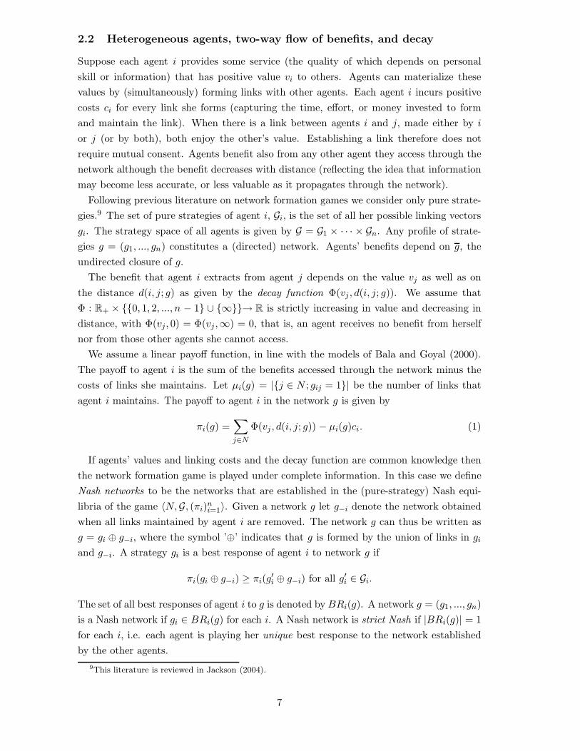
We also study the more complex situation with one low-cost agent ic, one high-valueagent iv, and n − 2 normal agents, using the parameters from the cases above. In all ourtreatments we study groups of n = 6 agents. Table 1 summarizes the parameter valuesused in our experiments.

Table 1: Experimental parameters.

a) Linking costs and values of different agent types.

cost per link made value to other agentsnormal agent 24 16

low cost agent 7 16high value agent 24 32

b) Benefits (per agent accessed) from accessing differenttypes of agents at different distances.

distance 1 2 3 4 5 ∞normal or low cost agent 16 12 9 7 5 0

high value agent 32 24 18 14 10 0

We investigate the network formation behavior in the four situations described aboveusing the following seven treatments (where the ‘I’ stands for complete and the ‘N’ forincomplete information):

(BI) baseline treatment with groups of 6 normal agents,

(CI & CN) treatments with groups of 5 normal agents and 1 low-cost agent,

(VI & VN) treatments with groups of 5 normal agents and 1 high-value agent, and

(CVI & CVN) treatments with groups of 4 normal agents, 1 low-cost agent, and 1 high-value agent.

Since we are particularly interested in the dynamics of network formation the networkformation game is repeated for 30 rounds within each group. In each round, subjects firstsimultaneously make their linking decisions and then each subject is informed about theestablished network, her total benefits, her costs, and her payoff. Groups and individualtypes are fixed throughout the experiment and in each group each subject keeps a uniqueidentification tag. In treatments BI, VI, CI, and CVI, the type of each agent is publiclyannounced at the beginning of the first round of the experiment. In treatments CN, VN,and CVN, the collection of types in the group is publicly announced at the beginning of

10

the first round of the experiment, but the type of each agent remains private informationthroughout the experiment. Treatments CN, VN, and CVN differ from treatments CI,VI, and CVI, respectively, only in terms of the quality of information. See Table 2 for anoverview.

Table 2: Group composition and information condition in each of our treatments.

complete information incomplete information6o BI (7) -5o + 1c CI (6) CN (6)5o + 1v VI (4) VN (6)4o + 1c + 1v CVI (4) CVN (6)

Note: Numbers of independent observations (i.e., groups) in parenthesis.

Abbreviations: o - normal agent, c - low-cost agent, v - high-value agent.

2.4 Experimental procedures

The experimental sessions were conducted in Spring of 2003 at the CREED laboratory atthe University of Amsterdam and at the Social Science Experimental Laboratory at theCalifornia Institute of Technology. In total 234 subjects participated. Each experimentalsession lasted between 45 and 90 minutes. Subjects’ total earnings were determined bythe sum of the points earned over all the rounds, using a conversion rate of 70 points perEuro or US dollar (the benefits and costs listed in Table 1 are all in points). The averageearnings were 22.8 Euros or (roughly) USD 25 at the time the experiments were conducted.Most subjects were economics or business administration undergraduates. They wererecruited through notices on bulletin boards and through email announcements. Eachsubject participated in only one session and none had previously participated in a similarexperiment. To ensure anonymity, at least twelve subjects were recruited for every sessionand were randomly divided into at least two independent groups. They were seated inseparated cubicles, which eliminated most possibilities for communication other than viathe computer network. We consider each group as one independent observation, see Table2 for numbers of groups in different treatments.

At the beginning of a session, subjects were told the rules of conduct and providedwith detailed instructions. The instructions were read aloud and shown on the computerscreen.13 After having finished the instructions, subjects received a printed summaryand were asked to complete a questionnaire designed to test their understanding of thenetwork formation game, the payoff calculations, and the computer interface. Once allsubjects had correctly answered the questionnaire, we conducted a single practice round(without providing feedback about others’ choices). The experiment started after allsubjects confirmed they had no further questions.

13The experiment and the questionnaire were computerized using software developed at CREED by Jos

Theelen.

11

Care was taken to minimize differences in the instructions for different treatments.14

In all treatments, subjects knew the size of their group, the numbers of normal, low-cost,and high-value types in their group, the type-conditional payoff functions, the informationcondition, and the number of rounds. To increase anonymity and avoid suggestive framing,each subject’s screen displayed herself as “Me” and the other five members in her group as“A”, “B”, “C”, “D”, and “E”. Each letter corresponded to the same member in the groupthroughout the session, and this was common knowledge. The game was neutrally framed:each subject was either “green” (normal), “purple” (low-cost), or “blue” (high-value) andwas forming “links” with other subjects. In the complete information treatments, eachsubject observed the color of all other subjects in the group. In the incomplete informationtreatments, each subject only observed her own color.

2.5 Equilibrium and efficiency analysis

For reference, subscripts c, v, and o, respectively, indicate a low-cost agent, a high-value,or a (normal) other agent in the center of a minimally-sponsored star MSSx, a periphery-sponsored star PSSx, or a center-sponsored star CSSx, where x can be c, v or o. LSp

cx

denotes a linked star with a low-cost agent in one center sponsoring links with p peripheryagents, and an agent of type x in the other periphery-sponsored center linked with 4 − p

periphery agents (LS1co, LS2

cv and LS1cv are shown in Figures 3d, 5c, and 5d, respectively).

PSS−v denotes a star with a normal agent in the center that is periphery-sponsored exceptfor the center sponsoring one link to the high-value agent (see Figure 4c).

Propositions 1 and 2 give complete characterizations of the (Bayesian) Nash networksfor the one-shot network formation games in each of our treatments. The proofs areprovided in the Appendix. Illustrations of the equilibrium networks are given in Figures2-5.

Proposition 1 The following are all Nash networks for the complete information treat-ments:BI: all PSS and the EN.VI: all PSS and all PSS−v.CI: all PSS, all MSSc including the CSSc, and all LS1

co.CVI: the PSSv, all MSSc including the CSSc, and all LS1

cv and LS2cv.

These networks are in all cases strict Nash.

Proposition 2 For the incomplete information treatments the following are all BayesianNash networks, given any feasible allocation of types:VN: all PSS and the EN.CN,CVN: all PSS, all MSSc including the CSSc, and all LS1

co and LS1cv.

These networks are in all cases strict Bayesian Nash.14Instructions can be found in Appendix B with the parts that differ between treatments emphasized. In-

structions for all treatments can be downloaded from http://www1.fee.uva.nl/creed/people/ule/index.htm.

12

���

��

���

�

��

���

�

� �

�����

�

a) PSS

�

�

�

�

�

�

b) EN

Figure 2: The (Bayesian) Nash networks for treatments BI and VN.

���

��

���

�

��

���

�

� �

�����

�

a) PSSo

ic

���

������

��

���

�

� ��

��

���

b) MSSc (incl. PSSc)

ic

���������

������

� ��

��

���

c) CSSc

ic

���

��

���

�

��

���

�

� �

�

d) LSco

ic

Figure 3: The (Bayesian) Nash networks for treatments CI, CN and CVN.

���

��

���

�

��

���

�

� �

�����

�

a) PSSo

iv

���

��

���

�

��

���

�

� �

�����

�

b) PSSv

iv

���

��

���

�

��

���

�

� �

�����

�

c) PSS−v

iv

Figure 4: Nash networks for treatment VI.

13

���

��

���

�

��

���

�

� �

�����

�

a) PSSv

ic iv

���

������

��

���

�

� ��

��

���

b) MSSc

iciv

���

��

���

�

��

���

�

��

���

�

c) LScv

ic iv

���

��

���

�

��

���

�

� �

�

d) LScv

ic iv

Figure 5: Nash networks for treatment CVI.

Predictions regarding the impact of information on network formation are obtained bycomparing the set of equilibrium networks across the treatments with identical type dis-tributions. Limiting the information changes the set of equilibrium networks in the treat-ments with a high-value agent, but not in the treatment with only one low-cost agent.This suggests, in particular, that behavior in CI should be similar to that in CN. Withrepetition, however, agents may overcome the uncertainty about types in any incompleteinformation treatment. We are therefore interested whether in later rounds behavior inan incomplete information treatment is similar to behavior in the corresponding completeinformation treatment.

Equilibrium networks differ with respect to payoff inequality, which we define as the ratiobetween the maximal and the minimal payoff in the network g, maxi∈N πi(g)/mini∈N πi(g).15

In equilibrium, the payoff inequality in treatments CI, CN, CVI and CVN is lowest inCSSc, while in treatments VI and VN it is lowest in PSS−v. The payoff inequality inCSSc in treatments CI and CN is almost equal to that in PSSv in treatments VI, VN,CVI and CVN.

Efficiency can be measured with the sum of agents’ payoffs. Let w : G → R be definedas w(g) =

∑ni=1 πi(g). A network g is efficient if w(g) ≥ w(g′) for all g′ ∈ G. For the linear

payoffs in equation (1) the efficient network is the one which maximizes the total benefitsof all agents, less the aggregate cost of links of the network. Proposition 3 shows thatstar networks have the best ratio between the number of links and the aggregate distancebetween agents.

15Payoff inequalities in some prominent star networks are: (CI,CN) 1.42 in CSSc, 2.00 in any PSS,

(VI,VN) 1.38 in PSS−v, 1.43 in PSSv, 2.40 in any PSSo, (CVI,CVN) 1.25 in CSSc, 1.43 in PSSv, 1.71

in PSS−v, 2.40 in any PSSo and PSSc.

14

Proposition 3 The following are all efficient networks for the different treatments.BI: all MSS.VI,VN: all MSSv.CI,CN,CVI,CVN: the CSSc.

The proof of Proposition 3 is provided in the Appendix. In treatment BI each periphery-sponsored star network is Nash and efficient. In all other treatments there is a uniqueefficient (Bayesian) Nash network. To summarize, in every treatment the efficient equilib-rium network is a star network. In order to assess how close to the efficient networks theactually formed networks come we define the relative efficiency of a network g ∈ G to bethe ratio w(g)/w(g∗), where g∗ ∈ G is the efficient network. The two benchmark relativeefficiencies are 0 for the empty network and 1 for the efficient network.

3 Results

We first present results concerning the occurrence of equilibrium networks in the differenttreatments. Then we investigate whether star networks are formed and how the frequencyof stars (if any) vary across treatments and over time. We briefly discuss the efficiency andstability of the observed networks. Finally, we study how individual behavior accountsfor the observed networks. For convenience we use the classification of star architecturesintroduced in section 2.1. If not otherwise stated all statistical tests are based on theindependent observations, i.e., groups.

We begin with a few preliminary observations. Subjects in our experiments activelylink with each other: across all treatments and all rounds we never observe the emptynetwork. Neither do we observe the complete network, which indicates that there is noexcessive ‘over-linking’. Furthermore, we observe that between 11% and 14% of networks intreatments BI, CI and CN are minimally connected whereas in treatments VI, VN, CVI andCVN their frequencies are between 43% and 60%. Since non-empty equilibrium networksare minimally connected (see Appendix) these frequencies suggest that the presence of ahigh-value agent facilitates formation of equilibrium networks.

3.1 Do subjects form equilibrium networks?

Table 3 depicts the frequency of (Bayesian) Nash networks in all treatments across allrounds. The differences across treatments are quite striking. In the baseline treatment BIwith only homogeneous agents not a single Nash network is formed. A similar conclusionholds for treatments with one low-cost agent. In CI and CN, respectively, only 2.2% and8.9% of all observed networks are (Bayesian) Nash. However, introducing a high-valueagent has a dramatic effect on the frequency of equilibrium networks. In VI and VN,40.8% and 51.1% of all observed networks are (Bayesian) Nash and for CVI and CVN thenumbers are 33.3% and 26.7% respectively.

Considering data from only the last five rounds indicates even larger differences acrosstreatments. The relative frequency of (Bayesian) Nash networks in VI, VN, CVI, and

15

CVN, respectively, is 75.0%, 83.3%, 95.0%, and 66.7%. In stark contrast, in CI and CNonly 10.0% and 16.7% of all networks are (Bayesian) Nash. In BI no Nash networks areformed at all. In the treatments where a high-value agent is present subjects tend to forman equilibrium network whereas this is not the case in the other treatments.16

Table 3: Frequency of (Bayesian) Nash networks in the different treatments.

Equilibrium networks

Treatment EN PSSo PSSv PSS−v MSSc LSco LScv Total # obs.

BI 0.0% 0.0% 0.0% 210

CI 0.0% 2.2% 0.0% 2.2% 180

CN 0.0% 8.9% 0.0% 8.9% 180

VI 0.0% 40.8% 0% 40.8% 120

VN 0.0% 0.0% 51.1% 51.1% 180

CVI 33.3% 0.0% 33.3% 120

CVN 0.0% 17.8% 5.0% 3.9% 26.7% 180

Note: PSSo (PSSv): periphery-sponsored star with a normal (high-value) type in the center;

PSS−v: star with a normal agent in the center that is periphery-sponsored except for the center

sponsoring one link to the high-value agent; MSSc: minimally-sponsored star with the low-cost

agent in the center; LSco (LScv): linked star with a low-cost agent in one center and a normal

(high-value) agent in the other center; EN: empty network. Empty cells indicate the network is

not an equilibrium network in the corresponding treatment.

3.2 Do subjects form star networks?

Figure 6 depicts the frequency of the different star architectures for all seven treatmentsaggregated across the first five rounds (panel(a)) and the last five rounds (panel (b)). Veryfew star structures are formed in early rounds. In treatments BI, CN, CVI and CVN, nostars are observed at all. In treatment CI only 10% (3/30) of all networks are stars, all ofthem have the low cost agent in the center with mixed sponsoring. Some stars are formedin the treatments with one high-value agent (25% (5/20) in VI and 10% (3/30) in VN).Interestingly, all observed star networks in VI and VN are efficient equilibrium networks,i.e. periphery-sponsored stars with the high-value agent in the center.

Figure 6(b) highlights the differences across treatments in the last five rounds. Com-paring the results to those for the first five rounds indicates that repetition and experience

16We calculated the Spearman rank order correlations between the average number of (Bayesian) Nash

networks across groups and the round number. For treatments VI, VN, CVI, and CVN this correlation

coefficient is larger than 0.86 and significant at p < 0.0001 (two-sided tests). This clearly indicates that

in these treatments more equilibrium networks are formed as agents gain experience. Interestingly, there

is weak evidence of learning in treatment CN, where the percentage of Bayesian Nash networks increases

from 0.0% in the first 16 rounds to 16.7% in the last few rounds. This increase is statistically significant

(ρ = 0.84, p < 0.0001; two-sided test). Note, however, that in quantitative terms the number of Bayesian

Nash networks in CN is considerably less than in treatments with a high-value agent. No convergence

towards Nash networks can be found in treatments BI (because there are no Nash networks at all) and CI

where the Spearman correlation coefficient is not significantly different from zero (p > 0.2935; two-sided

tests).

16

0.1

.2.3

.4.5

.6.7

.8.9

1re

lativ

e fr

eque

ncy

of d

iffer

ent s

tars

BI CI CN VI VN CVI CVN

PSS_vCSS_cstar_vstar_cgeneral starother networks

(a) Rounds 1-5

0.1

.2.3

.4.5

.6.7

.8.9

1re

lativ

e fr

eque

ncy

of d

iffer

ent s

tars

BI CI CN VI VN CVI CVN

PSS_vCSS_cstar_vstar_cgeneral starother networks

(b) Rounds 26-30

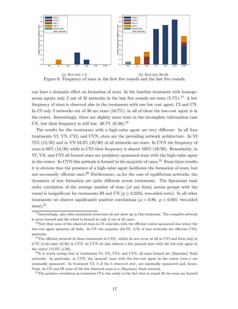
Figure 6: Frequency of stars in the first five rounds and the last five rounds.

can have a dramatic effect on formation of stars. In the baseline treatment with homoge-neous agents only 2 out of 35 networks in the last five rounds are stars (5.7%).17 A lowfrequency of stars is observed also in the treatments with one low cost agent, CI and CN.In CI only 5 networks out of 30 are stars (16.7%); in all of them the low-cost agent is inthe center. Interestingly, there are slightly more stars in the incomplete information caseCN, but their frequency is still low: 26.7% (8/30).18

The results for the treatments with a high-value agent are very different. In all fourtreatments VI, VN, CVI, and CVN, stars are the prevailing network architecture. In VI75% (15/20) and in VN 83.3% (25/30) of all networks are stars. In CVN the frequency ofstars is 60% (18/30) while in CVI their frequency is almost 100% (19/20). Remarkably, inVI, VN, and CVI all formed stars are periphery sponsored stars with the high-value agentin the center. In CVN this network is formed in the majority of cases.19 From these resultsit is obvious that the presence of a high-value agent facilitates the formation of stars, butnot necessarily efficient ones.20 Furthermore, as for the case of equilibrium networks, thedynamics of star formation are quite different across treatments. The Spearman rankorder correlation of the average number of stars (of any form) across groups with theround is insignificant for treatments BI and CN (p ≥ 0.2255; two-sided tests). In all othertreatments we observe significantly positive correlations (ρ > 0.80, p < 0.001; two-sidedtests).21

17Interestingly, also other prominent structures do not show up in this treatment. The complete network

is never formed and the wheel is formed in only 2 out of 35 cases.18Note that none of the observed stars in CI coincides with the efficient center-sponsored star where the

low-cost agent sponsors all links. In CN the majority (62.5%; 5/8) of star networks are efficient CSSc

networks.19The efficient network in these treatments is CSSc, which do not occur at all in CVI and form only in

6.7% of all cases (2/30) in CVN. In CVN we also observe a few general stars with the low-cost agent in

the center (13.3%; 4/30).20It is worth noting that in treatments VI, VN, CVI, and CVN, all stars formed are (Bayesian) Nash

networks. In particular, in CVN, the ‘general’ stars with the low-cost agent in the center (starc) are

minimally sponsored. In treatment CI, 3 of the 5 observed starc are minimally sponsored and, hence,

Nash. In CN and BI none of the few observed stars is a (Bayesian) Nash network.21The positive correlation in treatment CI is due solely to the fact that in round 29 two stars are formed

17

To summarize, stars (whether equilibrium or not) very rarely form in early rounds whensubjects have little or no experience (independent of the treatment). This indicates thatforming a star with a high-value or a low-cost agent in the center is not an obvious or focaloutcome. With repetition, only a few stars are formed when agents are homogeneous ordiffer only in linking costs. In contrast, in treatments with a high-value agent, experiencedagents often form stars, most frequently with the high-value agent in the center.

Given that stars only form in some of the treatments, asking for ‘exact’ stars maybe too restrictive given the huge coordination problem subjects face in the experiment.We therefore also investigate two less restrictive measures: one is based on the notion of‘almost-stars’ and the other is based on the ‘centrality’ of a network.

Almost stars: close-to-star networks, or almost stars, are defined as networks that canbe transformed into a star by deleting, adding, or moving a single link. Table 4 depictsthe relative and absolute frequencies of general stars and general almost-stars in the seventreatments. The results are akin to those for exact stars. There are more almost starsin later rounds than in earlier rounds and the frequencies of these network structures isclearly largest in treatments where a high-value agent is present. However, there are alsosome interesting differences compared to the more restrictive exact-star measure. In earlyrounds of treatment BI there are still only a few almost stars (5.7%), but in the last fiverounds their frequency increases to 31.4%. Thus, although subjects almost completely failto form exact stars it seems that with experience they form almost-stars to some extent.This pattern is more pronounced in treatment CN, where in early rounds only 3.3% of allnetworks are almost stars and this frequency increases to 56.7% in the last five rounds.No such pattern is observed in treatment CI. This corroborates the earlier finding that intreatments with only a low-cost agent incomplete information facilitates the formation of(almost) stars. It also further confirms that forming stars with the distinctive agent in thecenter is not an obvious or focal outcome.

Table 4: Frequency of stars and almost stars (of any form) in the different treatments.

Treatment rounds 1-5 rounds 26-30 all rounds

BI 5.7% (2/35) 31.4% (11/35) 15.2% (32/210)

CI 23.3% (7/30) 36.7% (11/30) 18.9% (34/180)

CN 3.3% (1/30) 56.7% (17/30) 35.0% (63/180)

VI 40.0% (8/20) 75.0% (15/20) 59.2% (71/120)

VN 13.3% (4/30) 83.3% (25/30) 61.1% (110/180)

CVI 0.0% (0/20) 100.0% (20/20) 56.7% (68/120)

CVN 6.7% (2/30) 90.0% (27/30) 51.7% (93/180)

The tendency towards star like structures in CVN and, especially, CVI is worth noting.In treatment CVN, in early rounds, only 6.7% of all networks are almost stars but in the

and in round 30 three stars are formed while in any of the previous rounds at most 1 star is observed. In

the other treatments with a significantly positive correlation coefficient the increase in the number of stars

over time exhibits a much stronger pattern.

18

last five rounds this frequency increases to 90%. For CVI we already saw that in the firstfive rounds no exact star is formed. Table 4 shows that in the early rounds not even analmost star is observed. Nevertheless, at the end of the game all but one network is a star(see above) and the remaining network turns out to be an almost star.

To test whether the changes in the frequencies of almost-star networks over time aresignificant we calculate Spearman rank order correlation statistics for all treatments. Fortreatments VI, VN, CN, CVI, and CVN the correlation coefficient is significantly greaterthan zero (ρ > 0.75, p < 0.0001; two-sided tests). For treatment BI the correlationturns out to be only marginally significant (ρ = 0.31, p = 0.0938; two sided test) andinsignificant for treatment CI (p = 0.4949; two-sided test).

To summarize, stars are observed mainly in later rounds and only in treatments witha high-value agent. When relaxing the criterion to almost stars, other treatments exhibitsome tendency towards star like structures, with the noticeable exception of treatmentsCI and BI.

Network centrality: the second measure we use to examine whether the observed net-works come close to stars is the centrality of a network. Individual centrality is a measurethat is often employed in sociological studies to analyze how central (strong, important)agents’ positions are in a network regarding, e.g., communication flow, interaction possi-bilities, or power.22 One can build upon the individual centrality measures to construct ameasure of centrality for the whole network. While various definitions are possible, we usethe so called ‘degree-centrality’ measure, which is defined as the sum of the differences indegrees between the most central agent and all other agents. Formally,

cent(g) =120

∑i∈N

[maxj∈N

degj(g) − degi(g)]

.

Important properties of degree-centrality (or other measures of centrality proposed in theliterature) are that it is bounded and, given our normalization, 0 for ‘even’ networks suchas the empty, complete, and wheel networks, and 1 if and only if the network is a star.Increasing centrality can be interpreted as a movement towards star or star-like networks.We are, therefore, particularly interested if the centrality measure increases over time andwhether it approaches 1.

Figure 7 depicts the development of average centrality in all seven treatments overrounds (in blocks of 5 rounds). It shows that in early rounds the centrality of networksis very similar across treatments, with the exception of treatment VI. Indeed, a Kruskal-Wallis equality of populations rank test does not reject the hypothesis that the centralitymeasures across the first five rounds are the same in all treatments (p = 0.5411). Thedevelopment of centrality differs strongly across treatments, however. For treatments CN,VI, VN, CVI, and CVN centrality clearly shows an upward trend. In contrast, in BI andCI no such tendency is observed. Restricting attention to the average centrality in the

22See e.g. Freeman (1979) and Wasserman and Faust (1994) for detailed discussions of centrality mea-

sures.

19

.3

.4

.5

.6

.7

.8

.9

1

netw

ork

cent

ralit

y

1 to 5 6 to 10 11 to 15 16 to 20 21 to 25 26 to 30round block

BI CICN VIVN CVICVN

Figure 7: Development of centrality over time.

last five rounds, a Kruskal-Wallis test rejects the hypothesis that centrality is the same inall treatments (p = 0.0044).23

To test whether the treatments network centrality approaches 1 we conducted Wilcoxonsigned-rank tests based on the network centrality averaged across the last five rounds.The null hypothesis is that network centrality is equal to 1. We reject this hypothesis fortreatments BI (p = 0.0178), CI (p = 0.0277), CN (p = 0.0350), and marginally also forCVN (p = 0.0523). In the other treatments, i.e., VI, VN, and CVI, we cannot reject thehypothesis (p ≥ 0.3173; all tests two-sided). Hence, our earlier conclusions regarding starformation in the different treatments are corroborated.

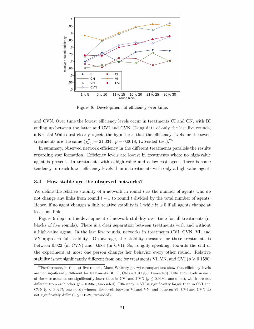
3.3 How efficient are the observed networks?

The prevalence of PSSv in CVI indicates that the formation of stars does not necessarilylead to efficient outcomes. In this treatment the CSSc network would be efficient butis never observed. Figure 8 shows the development of the relative efficiency of observednetworks for the different treatments aggregated over blocks of five rounds. Clearly, effi-ciency in early rounds (rounds 1-5) is similar across treatments (only in VI more efficientnetworks are formed).24 Figure 8 shows that relative efficiencies in treatments VI and VNincrease and converge to a common level. A similar pattern holds for treatments CVI

23Pairwise comparisons using Mann-Whitney tests show that equality of centrality in BI and CI can not

be rejected (p = 0.2827; two-sided test) and that centrality in VI, VN, CVI, and CVN is higher than in BI

and CI (all comparisons at the 5 percent significance level, except for CI vs. VI where p = 0.084; two-sided

tests).24This impression is corroborated by a Kruskal-Wallis test for equality of populations between all treat-

ments except VI (χ2(5) = 4.575, p = 0.4699, two-sided test). Mann-Whitney tests comparing (pairwise)

early-round efficiency in VI with other treatments shows significant differences in all cases at least at the

5 percent level, except for VI vs. VN where the difference is only marginally significant (p = 0.0550; all

tests two-sided).

20

.5

.55

.6

.65

.7

.75

.8

.85

.9

.95

1

rela

tive

netw

ork

effic

ienc

y

1 to 5 6 to 10 11 to 15 16 to 20 21 to 25 26 to 30round block

BI CICN VIVN CVICVN

Figure 8: Development of efficiency over time.

and CVN. Over time the lowest efficiency levels occur in treatments CI and CN, with BIending up between the latter and CVI and CVN. Using data of only the last five rounds,a Kruskal-Wallis test clearly rejects the hypothesis that the efficiency levels for the seventreatments are the same (χ2

(6) = 21.034, p = 0.0018, two-sided test).25

In summary, observed network efficiency in the different treatments parallels the resultsregarding star formation. Efficiency levels are lowest in treatments where no high-valueagent is present. In treatments with a high-value and a low-cost agent, there is sometendency to reach lower efficiency levels than in treatments with only a high-value agent.

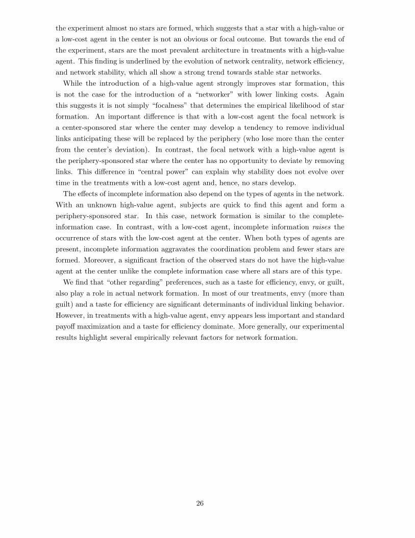
3.4 How stable are the observed networks?

We define the relative stability of a network in round t as the number of agents who donot change any links from round t − 1 to round t divided by the total number of agents.Hence, if no agent changes a link, relative stability is 1 while it is 0 if all agents change atleast one link.

Figure 9 depicts the development of network stability over time for all treatments (inblocks of five rounds). There is a clear separation between treatments with and withouta high-value agent. In the last few rounds, networks in treatments CVI, CVN, VI, andVN approach full stability. On average, the stability measure for these treatments isbetween 0.922 (in CVN) and 0.983 (in CVI). So, roughly speaking, towards the end ofthe experiment at most one person changes her behavior every other round. Relativestability is not significantly different from one for treatments VI, VN, and CVI (p ≥ 0.1590;

25Furthermore, in the last five rounds, Mann-Whitney pairwise comparisons show that efficiency levels

are not significantly different for treatments BI, CI, CN (p ≥ 0.1985; two-sided). Efficiency levels in each

of these treatments are significantly lower than in CVI and CVN (p ≤ 0.0430; one-sided), which are not

different from each other (p = 0.3367; two-sided). Efficiency in VN is significantly larger than in CVI and

CVN (p < 0.0297; one-sided) whereas the levels between VI and VN, and between VI, CVI and CVN do

not significantly differ (p ≤ 0.1939; two-sided).

21

.1

.2

.3

.4

.5

.6

.7

.8

.9

1

netw

ork

stab

ility

1 to 5 6 to 10 11 to 15 16 to 20 21 to 25 26 to 30round block

BI CICN VIVN CVICVN

Figure 9: Development of network stability over time.

two-sided Wilcoxon signed-rank test). In treatment CVN relative stability is also largebut marginally different from one (p ≥ 0.0516; two-sided Wilcoxon signed-rank test),indicating that network formation did not completely settle down.

In the treatments without a high-value agent, networks remain unstable over time andthere is no tendency towards stability. In the last five rounds, average relative stabilityis between 0.467 (in BI) and 0.622 (in CN), meaning that on average between 2.3 and3.2 agents change behavior in each round. In the last five rounds, stability does notsignificantly differ across treatments BI, CI, and CN (χ2

(2) = 3.018, p = 0.2211; Kruskal-Wallis test, two-sided). Mann-Whitney tests show that compared to the treatments witha high-value agent, stability is significantly smaller (pair-wise comparisons: p < 0.05 in allcases except CN vs. VI where p = 0.0521; two-sided tests).

In summary, network stability strongly improves in the presence of a high-value agentand networks reach (almost) full stability at the end of the experiment. In stark contrast,networks remain unstable in treatments without a high-value agent.

3.5 Determinants of individual linking behavior

The observed network structures are ultimately the outcome of individual linking decisions.To understand why the observed networks are so different across treatments - unlike thetheoretical predictions - we study possible determinants of individual behavior.

Recent models of generalized preferences assume that subjects’ behavior not only de-pends on their material income but also on their relative standing towards others (e.g.,Fehr and Schmidt (1999) and Bolton and Ockenfels (2000)).26 In addition, behavior maybe influenced by the “well-being” of the relevant reference group as a whole. Charness

26Fehr and Schmidt (1999) model agent i’s utility, given a profile of monetary payoffs (x1, . . . , xi, . . . , xn),

as u(x1, . . . , xi, . . . , xn) = xi − αin−1

�j �=i max{xj −xi, 0}− βi

n−1

�j �=i max{xi −xj , 0}, where αi is an envy

coefficient and βi a guilt coefficient.

22

and Rabin (2002) incorporate the latter idea in their model as a “concern for efficiency.”Both motives, inequality aversion and efficiency concerns, may have consequences for thenetwork formation process. Indeed, Falk and Kosfeld (2005) find evidence for inequalityaversion being an important reason for the absence of stars in their experiments. Ex-tending their ideas we investigate if linking behavior is influenced by envy, guilt and/orefficiency concerns. Like Falk and Kosfeld (2005), we control for standard best-replybehavior, which may also be interpreted as a proxy for the influence of a subject’s ownearnings on behavior. We conduct probit regressions to examine how a subjects’ likelihoodto stick to the same choice in round t as in round t− 1 depends on their relative standingtowards others in the group as well as total group earnings, where we control for previousbest-reply play and time (assuming a linear trend). We conduct these regressions for alltreatments but pool the data of the complete and incomplete information conditions, andmeasure its effect with a dummy variable. Since we observe very different networks inthe different treatments, we are particularly interested whether individual behavior differsacross treatments and agent types.

More precisely, we estimate the following probit regression separately for the differentheterogeneity conditions (pooled over information conditions):27

P(no changei,t) = Φ(α0 + α1,i BR(t − 1)i + α2,i eff(t − 1) +

α3,i envy(t − 1)i + α4,i guilt(t − 1)i + α5 t + α6 info),

Table 5 displays the results of the regression analysis. Note that in all treatments, normalagents (o) have a strong tendency to stick to their previous round behavior if this was abest reply. This indicates that individual earnings maximization is an important motivefor normal agents in all treatments.28 Individual earnings also seem important for high-value agents (see the results for treatments VI&VN and CVI&CVN). For the low-costagent, results are less clear-cut. In CVI&CVN these agents show a significant tendency tostick to their behavior if it was best-reply in the last round but this is not the case whenno high-value agent is present.

Concern for efficiency is an important motive for all agent types. For normal (high-value) agents the regression coefficient for our efficiency measure is significantly positivein all treatments (where they are present). For low-cost types the corresponding coefficientis (marginally) significant when a high-value type is present but seems to be unimportantif this is not the case.

27Here i = o, c, v denotes the agent type (normal, low-cost, and high-value respectively), t denotes the

round number, and no changei,t is 1 if i made the same links in round t as in round t− 1 and 0 otherwise.

On the right hand side, Φ(·) denotes the standard normal cumulative, BR(t−1)i equals 1 if agent i played

a best response in round t − 1 and 0 otherwise, eff(t − 1) equals the sum of earnings in agent i’s group

in round t − 1, envy(t − 1)i is defined as 15

�j max{xj − xi, 0} and guilt(t − 1)i as 1

5

�j max{xi − xj , 0}

where xj is subject j’s monetary payoff, and, finally, info equals 1 for the complete information treatment

and 0 otherwise. Best responses in the latter treatments are computed as if agents’ types are known, since

subjects in the experiment were able to resolve the incomplete information about types fast.28This motive appears strongest in the treatments with a high-value agent (VI&VN and CVI&CVN).

The coefficients for these treatments are about twice as large as for BI and CI&CN.

23

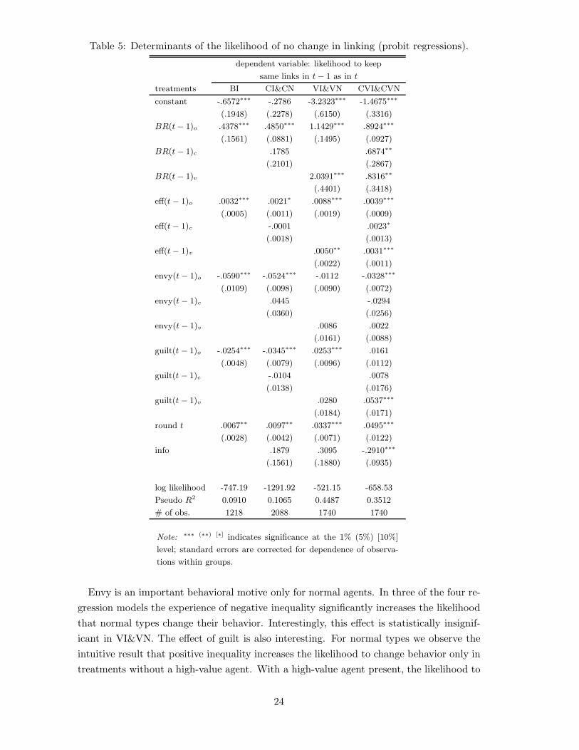
Table 5: Determinants of the likelihood of no change in linking (probit regressions).

dependent variable: likelihood to keep

same links in t − 1 as in t

treatments BI CI&CN VI&VN CVI&CVN

constant -.6572∗∗∗ -.2786 -3.2323∗∗∗ -1.4675∗∗∗

(.1948) (.2278) (.6150) (.3316)

BR(t − 1)o .4378∗∗∗ .4850∗∗∗ 1.1429∗∗∗ .8924∗∗∗

(.1561) (.0881) (.1495) (.0927)

BR(t − 1)c .1785 .6874∗∗

(.2101) (.2867)

BR(t − 1)v 2.0391∗∗∗ .8316∗∗

(.4401) (.3418)

eff(t − 1)o .0032∗∗∗ .0021∗ .0088∗∗∗ .0039∗∗∗

(.0005) (.0011) (.0019) (.0009)

eff(t − 1)c -.0001 .0023∗

(.0018) (.0013)

eff(t − 1)v .0050∗∗ .0031∗∗∗

(.0022) (.0011)

envy(t − 1)o -.0590∗∗∗ -.0524∗∗∗ -.0112 -.0328∗∗∗

(.0109) (.0098) (.0090) (.0072)

envy(t − 1)c .0445 -.0294

(.0360) (.0256)

envy(t − 1)v .0086 .0022

(.0161) (.0088)

guilt(t − 1)o -.0254∗∗∗ -.0345∗∗∗ .0253∗∗∗ .0161

(.0048) (.0079) (.0096) (.0112)

guilt(t − 1)c -.0104 .0078

(.0138) (.0176)

guilt(t − 1)v .0280 .0537∗∗∗

(.0184) (.0171)

round t .0067∗∗ .0097∗∗ .0337∗∗∗ .0495∗∗∗

(.0028) (.0042) (.0071) (.0122)

info .1879 .3095 -.2910∗∗∗

(.1561) (.1880) (.0935)

log likelihood -747.19 -1291.92 -521.15 -658.53

Pseudo R2 0.0910 0.1065 0.4487 0.3512

# of obs. 1218 2088 1740 1740

Note: ∗∗∗ (∗∗) [∗] indicates significance at the 1% (5%) [10%]

level; standard errors are corrected for dependence of observa-

tions within groups.

Envy is an important behavioral motive only for normal agents. In three of the four re-gression models the experience of negative inequality significantly increases the likelihoodthat normal types change their behavior. Interestingly, this effect is statistically insignif-icant in VI&VN. The effect of guilt is also interesting. For normal types we observe theintuitive result that positive inequality increases the likelihood to change behavior only intreatments without a high-value agent. With a high-value agent present, the likelihood to

24

stick to the current behavior is positively related to guilt and this effect is highly signifi-cant in VI&VN but insignificant in CVI&CVN. A similar result is observed for high-valuetypes: in CVI&CVN we find a significantly positive effect of guilt while in VI&VN theguilt coefficient is insignificant.

In all treatments, a subject’s likelihood to stick to her previous round behavior signif-icantly increases over time, indicating that behavior stabilizes with repetition. Finally,the information dummy is significant only in CVI&CVN, consistent with the differencesin observed equilibrium networks and star-like architectures (Table 3 and Figure 6).

The main lesson to be taken from these results is that linking behavior depends on anagent’s own type and the types of other agents in the network. In particular, standardincome maximization is a prominent concern for all types of agents only when the high-value agent is present. Likewise, efficiency considerations are important for all types whena high-value agent is present, while this is not the case when the low-cost agent is the only‘different’ type in the group. Finally, envy is generally important for normal types butnot when faced with opportunity to link to a high-value agent.29

4 Conclusion

This paper reports the first experimental study on endogenous network formation withheterogeneous agents. We consider several implementations of individual heterogeneityand allow agents’ types to be private information or publicly known. Our simple para-metrization of agent heterogeneity simplifies the analysis of equilibrium networks andallows us to measure the effects of a small change in agent types. We provide a completecharacterization of the set of (Bayesian) Nash equilibria for all treatments and considerapproximations in terms of “almost star networks and by measuring network centrality.Our interest in doing the experiments is not simply in testing theory. Indeed, the mainmotivation for this work is to uncover factors that are relevant in actual network formation.

Casual empiricism suggests that individual differences may facilitate the creation ofuneven, hierarchal structures such as star networks. Some people have lower opportunitycosts or a taste for networking, while others may possess skills or information that isrelatively more scarce. We conjectured that the presence of these “special” individualsfacilitates the creation of star-type networks because it reduces the coordination problemand makes the resulting payoff inequalities more acceptable.

The experimental results corroborate this intuition. We find that almost no stars formamong symmetric agents. In contrast, the introduction of different types of agents has adramatic impact on linking behavior and observed networks: stars are prevalent in mostheterogeneous treatments. Stars are not born, however, but grow over time. Early on in

29We also estimated a model where agents make logit best-responses against the previous round network.

We find similar levels of noise in the baseline and CVI&CVN treatments (µ = 9.0 and µ = 8.7 respectively)

but lower levels in the VI&VN and CVI&CVN treatments (µ = 4.5 and µ = 2.2). When the basic logit

model is “dressed up” with other-regarding preferences, the estimated envy and guilt parameters vary

across treatments, like in Table 5.

25

the experiment almost no stars are formed, which suggests that a star with a high-value ora low-cost agent in the center is not an obvious or focal outcome. But towards the end ofthe experiment, stars are the most prevalent architecture in treatments with a high-valueagent. This finding is underlined by the evolution of network centrality, network efficiency,and network stability, which all show a strong trend towards stable star networks.

While the introduction of a high-value agent strongly improves star formation, thisis not the case for the introduction of a “networker” with lower linking costs. Againthis suggests it is not simply “focalness” that determines the empirical likelihood of starformation. An important difference is that with a low-cost agent the focal network isa center-sponsored star where the center may develop a tendency to remove individuallinks anticipating these will be replaced by the periphery (who lose more than the centerfrom the center’s deviation). In contrast, the focal network with a high-value agent isthe periphery-sponsored star where the center has no opportunity to deviate by removinglinks. This difference in “central power” can explain why stability does not evolve overtime in the treatments with a low-cost agent and, hence, no stars develop.

The effects of incomplete information also depend on the types of agents in the network.With an unknown high-value agent, subjects are quick to find this agent and form aperiphery-sponsored star. In this case, network formation is similar to the complete-information case. In contrast, with a low-cost agent, incomplete information raises theoccurrence of stars with the low-cost agent at the center. When both types of agents arepresent, incomplete information aggravates the coordination problem and fewer stars areformed. Moreover, a significant fraction of the observed stars do not have the high-valueagent at the center unlike the complete information case where all stars are of this type.

We find that “other regarding” preferences, such as a taste for efficiency, envy, or guilt,also play a role in actual network formation. In most of our treatments, envy (more thanguilt) and a taste for efficiency are significant determinants of individual linking behavior.However, in treatments with a high-value agent, envy appears less important and standardpayoff maximization and a taste for efficiency dominate. More generally, our experimentalresults highlight several empirically relevant factors for network formation.

26

References

Bala, V. and Goyal, S. (2000). A non-cooperative model of network formation. Econo-metrica, 68:1131–1230.

Barabasi, A.-L. (2002). Linked: The New Science of Networks. Promeus.

Barabasi, A.-L. and Albert, R. (1999). Emergence of scaling in random networks. Science,286(286):509–512.

Bolton, G. and Ockenfels, A. (2000). ERC - a theory of equity, reciprocity and altruism.American Economic Review, 90:166–193.

Callander, S. and Plott, C. (2005). Principles of network development and evolution: Anexperimental study. Journal of Public Economics, 89:1469–1495.

Charness, G. and Rabin, M. (2002). Understanding social preferences with simple tests.Quarterly Journal of Economics, 117:817–869.

Corbae, D. and Duffy, J. (2003). Experiments with network economies. mimeo.

Falk, A. and Kosfeld, M. (2005). It’s all about connections: Evidence on network forma-tion. Working paper, University of Zurich.

Fehr, E. and Schmidt, K. M. (1999). A theory of fairness, competition, and cooperation.The Quarterly Journal of Economics, 114:817–868.

Freeman, L. (1979). Centrality in social networks: Conceptual clarification. Social Net-works, 1:215–239.

Fudenberg, D. and Tirole, J. (1991). Game Theory. MIT Press, Cambridge, Massachusetts.

Galeotti, A., Goyal, S., and Kamphorst, J. (2005). Network formation with heterogeneousplayers. Games and Economic Behavior. Forthcoming.

Goyal, S., van der Leij, M., and Moraga-Gonzales, J. L. (2004). Economics: An emergingsmall world? mimeo.

Haller, H., Kamphorst, J., and Sarangi, S. (2006). (non-)existence and scope of nashnetworks. Forthcoming.

Haller, H. and Sarangi, S. (2005). Nash networks with heterogeneous links. MathematicalSocial Sciences, 50:181–201.

Jackson, M. O. (2004). A survey of models of network formation: Stability and efficiency.In Demange, G. and Wooders, M., editors, Group Formation in Economics: Networks,Clubs and Coalitions. Cambridge University Press, Cambridge.

27

Jackson, M. O. (2005). The economics of social networks. In Blundell, R., Newey, W., andPersson, T., editors, Proceedings of the 9th World Congress of the Econometric Society.Cambridge University Press, Cambridge.

Jackson, M. O. and Rogers, B. (2005). Search in the formation of large networks: Howrandom are socially generated networks? mimeo.

Jackson, M. O. and Wolinsky, A. (1996). A strategic model of social and economic net-works. Journal of Economic Theory, 71:44–74.

Johnson, C. and Gilles, R. P. (2000). Spatial social networks. Review of Economic Design,5:273–299.

Kosfeld, M. (2004). Economic networks in the laboratory: A survey. Review of NetworkEconomics, 3:20–42.

McBride, M. (2005). Position-specific information in social networks: Are you connected?mimeo.

Newman, M. E. J. (2004). Coautorship networks and patterns of scientific collaboration.Proceedings of the National Academy of Sciences, 101:5200–5205.

Wasserman, S. and Faust, K. (1994). Social Network Analysis: Methods and Applications.Cambridge University Press.

28

A Appendix: Proofs.

In Lemma 4 below we characterize for each incomplete information treatment the expectedpayoff of each agent in each possible network. We next use this characterization to showin Proposition 5 below that all (Bayesian) Nash networks in all treatments are eitherminimally connected or empty. With the help of Lemma 4 and Proposition 5 we thenprove Propositions 1, 2 and 3.

The decay function used in our experiments can be expressed as Φ(vi, d) = viν◦(d)

16 , with ν

given by (ν◦(1), ν◦(2), ν◦(3), ν◦(4), ν◦(5), ν◦(∞)) = (16, 12, 9, 7, 5, 0), see Table 1b. Hence,the benefit from accessing a normal value agent at distance d is Φ(16, d) = ν◦(d), while thebenefit from accessing a high-value agent at the same distance is Φ(32, d) = 2ν◦(d). Thefollowing Lemma characterizes an agent’s expected payoff in the incomplete informationtreatments.

Lemma 4 Given a cost/value profile θ, the expected payoffs of different types of agentsin the incomplete information treatments are:1. for i �= iv in VN and CVN: Eiui(g; θi) = 6

5

∑j �=i ν

◦(d(i, j; g)) − µi(g)c,2. for iv in VN and CVN and for any i in CN: Eiui(g; θi) =

∑j �=i ν

◦(d(i, j; g)) − µi(g)c.

Proof. Note from (2) that agent i’s payoff is independent of the linking costs incurredby other agents j �= i. Agent i’s expected payoff therefore depends only on her beliefsabout others’ values.

1. Given the realized profile θ, any agent i �= iv in treatments VN and CVN knows thatany of the other agents is equally likely to be the unique high-value agent. For each k �= i,let wk = (wk

1 , ..., wkn) be one of the five possible value profiles from i’s perspective, with

wkk = 32 and wk

j = 16 for j �= k, and pθii [wk] = 1

5 . Agent i’s expected payoff, given thenetwork g, is

Eiui(g; θi) =∑k �=i

pθii [wk]

∑j �=i

Φ(wkj , d(i, j; g)) − µi(g)ci(θ)

=∑k �=i

15

∑j �=i

wkj

16ν◦(d(i, j; g)) − µi(g)ci =

180

∑j �=i

ν◦(d(i, j; g))∑k �=i

wkj − µi(g)ci

=180

∑j �=i

ν◦(d(i, j; g))96 − µi(g)ci =65

∑j �=i

ν◦(d(i, j; g)) − µi(g)ci.

2. Given the realized profile θ, all agents in treatment CN and agent iv in treatmentsVN and CVN know the value of any other agent is 16. Hence, for these agents theexpected payoff, given the network g, is Eiui(g; θi) =

∑j �=i Φ(16, d(i, j; g)) − µi(g)ci =∑

j �=i ν◦(d(i, j; g)) − µi(g)ci.

Proposition 5 With complete or incomplete information, (Bayesian) Nash networks areeither minimally connected or empty.

29

Proof. It is easy to see that a (Bayesian) Nash network is minimally sponsored: anagent incurs costs but no additional benefits from making a link to another agent whoalready maintains this link. It is also straightforward to see that whenever a link is madebetween i �= j, any other agent k that does not access i or j is willing to sponsor a linkwith either of them. This implies that a (Bayesian) Nash network is either empty orconnected. Next we show that such a network has no cycles. We do this by arguing thatin any minimal cycle there is at least one agent who benefits from removing a link fromthe cycle. Below we use the notation ij to denote a link made by i to j.

Treatments BI,VI,CI: Let g be a minimally sponsored network with a shortest circle oflength k ≥ 3. It is easy to see that in any such circle at least one link must be sponsoredby an agent of normal linking cost whose distance to the high-value agent (if present) doesnot change if she removes that link. Let (1, ..., k, 1) denote such a circle and 1k be thecorresponding link. Recall that the linking cost of (normal) agent 1 is c = 24.

If 1 removes the link 1k, yielding the network g−1k, the distances between her andother agents may increase, which lowers agent 1’s benefits. It is convenient to define∆ν◦(d,∆d) = ν◦(d) − ν◦(d + ∆d) as the loss in benefits that result when the distance (toa normal agent) increases from d to ∆d. The loss function ∆ν◦(d,∆d) is decreasing ind and increasing in ∆d. For each j, let ∆ikd(i, j; g) = d(i, j; g−ik) − d(i, j; g) denote theincrease in the distance between i and j when link ik is removed from g, and let

∆kπi(g) = πi(g) − πi(g−ik)

= ci +∑j �=i

vj

16[ν◦(d(i, j; g)) − ν◦(d(i, j; g−ik))]

= ci −∑j �=i

vj

16∆ν◦(d(i, j; g),∆ikd(i, j; g))

denote the corresponding change in agent i’s payoff. When agent 1 removes the link 1k, thedistances between herself and agents {2, ..., ⌈ k

2

⌉} remains the same, but the distances toall (normal-valued) other agents may increase. Her distance to any agent j > k increasesby at most k − 2, hence ∆ν◦(2, k − 2) is the maximum possible decrease in benefits for i

obtained from a normal agent j with whom i did not have a direct link in g. The changeof agent 1’s payoff, when she removes the link 1k, is therefore bounded by

∆kπ1(g) ≥ 24 −k∑

j= k2�+1

[ν◦(j − 1) − ν◦(k − j + 1)] − (n − k)∆ν◦(2, k − 2). (4)

For k = 3, 4, 5, 6 this bound is strictly positive (∆3π1(g) ≥ 11, ∆4π1(g) ≥ 7, ∆5π1(g) ≥ 5,∆6π1(g) ≥ 8), which implies that agent 1 always benefits from removing the link 1k.

Treatment CVI: In a Nash network the low-cost agent ic will always be linked with thehigh-value agent iv. Indeed, ic is willing to sponsor the link with iv in any minimally spon-sored g as the loss from removing such a link is at least 2∆ν◦(d(ic, iv ; g),∆dic,iv(ic, iv; g)) ≥

30

2∆ν◦(1, 1) = 8, which exceeds ic’s linking cost of 7. Since ic and iv are linked, in anycircle of length k ≥ 4 at least one link is sponsored by a normal agent whose distanceto the high-value agent (if present) does not change if she removes that link. The sameconclusion holds for a circle of length k = 3 where either ic or iv is not part of the circle.In both situations, the proof that applied to the BI, VI, and CI cases can be replicated.

Finally, suppose that both ic and iv are part a cycle of length k = 3, including a normalagent i who sponsors the link with iv.30 By removing this link agent i gains at least∆ivπi(g) ≥ 24 − (32/16) [ν◦(2) − ν◦(1)] − 3∆ν◦(2, 1) = 7.

Treatments VN,CN,CVN: Let θ be a feasible allocation of types. Lemma 4 implies that,compared to the complete information case, normal agents’ benefits are multiplied byfactor 6/5 in treatments VN and CVN while they are unchanged in treatment CN. Define∆kEiui(g; θi) = Eiui(g; θi) − Eiui(g−ik; θi). Again, let (1, ..., k, 1) be the shortest cyclein g and let agent 1 satisfy the asssumptions above. Following the steps of the proof fortreatment BI, inequality (4) becomes

∆kE1u1(g; θ1) ≥ 24 − 65

k∑j= k

2�+1

[ν◦(j − 1) − ν◦(k − j + 1)] − 65(n − k)∆ν◦(2, k − 2).

for treatments VN and CVN. The corresponding bounds (∆3E1u1(g; θ1) ≥ 8.4, ∆4E1u1(g; θ1) ≥3.6, ∆5E1u1(g; θ1) ≥ 1.2, ∆6E1u1(g; θ1) ≥ 4.8) are all strictly positive. For treatment CNthe bounds found in the proof for treatment BI apply.

Proof of Proposition 1. We leave it to the reader to verify that the listed networksare strict Nash. Note that the benefit to a normal cost agent for making a link with anisolated normal value agent is 16 and the cost is 24. In a Nash network (hereafter NN)the normal cost agent therefore never links to a normal periphery agent.

Next consider two distinct periphery agents i and j, each being the sponsor of their(only) link. Let i be linked to i1 and j be linked to j1 �= i1. If the network is Nash,agent i must find linking to i1 at least as beneficial as linking to j1. If j removes her linkwith j1 then agent i should find linking to i1 strictly more beneficial than linking to j1.But then agent j should find linking to i1 also strictly more beneficial than linking to j1,which contradicts the assumption that the network is Nash. Thus in a Nash network allperiphery agents who sponsor their only link are linked to the same central agent.

This provides some intuition for the predominance of periphery-sponsored stars amongthe NN. The rest of the proof proceeds by considering each treatment separately. Propo-sition 5 implies that, in a non-empty NN, each pair of agents is connected by a singlepath.

Treatment BI: Let g be a non-empty, minimally connected NN. The two agents i and j

who are furthest apart in g must be periphery and therefore sponsor their own link. Theymust therefore be linked to the same agent, which implies that 2 is the maximal distance

30If link ivi is sponsored by iv, then the proof above applies.

31

between agents in g. The star network is the only minimally connected network withmaximal distance of 2. The only non-empty NN is therefore the periphery-sponsored star.

Treatment VI: Let g be a NN. Normal agents are always willing to sponsor a link with anisolated iv so g cannot be empty. Let i and j be the two periphery agents who are furthestapart in g. Either both sponsor their own link and g is a star network, or one of them isiv. Let the path (iv , i1, ..., j1, j) be the longest path in g. If i1 �= j1 then j decreases theaverage distance to other agents by removing the link with j1 and making a link with i1.Therefore i1 = j1, the maximal distance is 2, and g is a star network in which all normalperiphery agents sponsor their link.

Treatment CI: Let g be a NN. Agent ic is willing to sponsor a link with any agent i who,in absence of such link, would be more than 2 links away or isolated. Hence g cannotbe empty. Let i and j be the two periphery agents who are furthest apart in g. If bothsponsor their own link then g is a star network. If the center of g is a normal agent theng is periphery-sponsored.

If d(i, j) ≥ 3 then agent ic must be sponsoring the link with either i or j, say withi. We argued above that d(ic, j) ≤ 2 for each j which, together with d(ic, i) = 1 impliesd(i, j) = 3. Let j be linked with j1. All other periphery agents sponsoring their own linkmust be linked with j1. Agent ic sponsors the links with all agents not linked to j1. Thisdefines the linked star LSp

icj1. It is easy to verify that if p ≥ 2 all other periphery agents

would prefer linking to ic. The star networks PSS and MSSc and the linked star LS1icj1

are the only NN.

Treatment CVI: Let g be a NN. Agent ic is willing to sponsor a link to iv regardless ofother links. Therefore, a star network with a normal agent in the center cannot be NN.If g is not a star then it is a linked star with agent ic in one center, see the proof fortreatment CI. If iv is a periphery agent linked with ic, all other agents would also linkwith ic, see the proof for treatment VI. Agent iv must therefore be in the other center ofthe linked star. It is easy to verify that g is NN if all or less than three periphery normalagents are linked with ic, which excludes all networks but the MSSc, and any LS2

cv, LS1cv

and LS0cv = PSSv.

Proof of Proposition 2. Again, we leave it to the reader to verify that the listednetworks are strict Bayesian Nash. The proof closely follows the steps in the proof ofProposition 1, using the expected payoffs characterized by Lemma 4. In particular, char-acterization of Bayesian Nash networks in treatment VN follows the same steps as thosefor treatment BI, and characterization of Bayesian Nash networks in treatments CN andCVN follows those for treatment CI.

Proof of Proposition 3. The sum of agents’ payoffs in a group can be written as

w(g) =∑

i,j∈N

Φ(vj, d(i, j; g)) −∑i∈N

µi(g)ci.

32

The efficient network therefore maximizes the aggregate benefits while minimizing thelinking costs, i.e. it minimizes the distances between agents using a minimal numberof links. Since adding a link to connect any two components of the network increasestotal payoffs, the efficient network is either empty or connected. In the latter case, it hasat least n − 1 links. Of the networks with precisely n − 1 links the star networks haveminimal average distances. In addition, the CSSc with the low-cost agent ic in the centerminimizes the aggregate linking costs, while a MSSv with the high-value agent iv in thecenter maximizes the aggregate benefits. One can verify that w(CSSc) > w(MSSv) whenboth ic and iv are present. Hence, among the star networks, CSSc is efficient whenever ic

is present and MSSv are efficient when only iv is present. Any MSS is the efficient starnetwork in BI. In a star network each new link benefits only the two linked agents. Addinglinks to the CSSc thus decreases total payoffs: each link costs 24 but adds only 4 to thepayoff of one agent and at most 8 to the payoff of the other (if one agent is a high-valueagent). Adding links to a MSSv or MSSo when ic is not present also decreases total payoffs.Finally, total payoffs decrease if links are removed from any MSS. The above-mentionedstar networks are therefore the efficient networks.

33

B Appendix: Instructions.

[Most of the text is the same for all treatments. Treatment-dependent text appears in italicsand in brackets ”[...]”, where we indicate the treatments in which the text appears.]

Welcome to this experiment in decision-making. In this experiment you can earn money.The amount of money you earn depends on the decisions you and other participants make.Please read these instructions carefully.

In the experiment you will earn points. At the end of the experiment we will convertthe points you have earned into US dollars [in Europe: ”euros”] according to the rate: 70

points equal $1 [in Europe: ”1 euro”]. You will be paid your earnings privately andconfidentially after the experiment.

Throughout the experiment you are not allowed to communicate with otherparticipants in any way. If you have a question please raise your hand. One

of us will come to your desk to answer it.

YOUR GROUPAt the beginning of the experiment the computer will randomly assign you - and all other

participants - to a group of 6 participants. Group compositions do not change duringthe experiment. Hence, you will be in the same group with the same people throughoutthe experiment. The composition of your group is anonymous. You will not get to knowthe identities of the other people in your group: neither during the experiment nor afterthe experiment. The other people in your group will also not get to know your identity.On your computer screen, you will be marked Me and each of the five other people in yourgroup will be marked with a letter: A, B, C, D, and E. Each letter will correspondto the same participant in your group during the entire experiment.

NUMBER OF ROUNDSThe experiment consists of 30 rounds. You will receive 150 points at the beginning of

the first round. In each round you can earn additional points. Your total earnings will bethe sum of the initial 150 points and your earnings in each of the 30 rounds.

YOUR LINKING DECISIONS (I)In each round you will make linking decisions. You will have the possibility to link with

any other participant in your group. That is, you can make any number of links (0, 1, 2,3, 4, or 5). The link(s) you make in a particular round are only valid for that

round.As we explain below, you can be “directly linked”, “indirectly linked” or “not

linked” with any other member of your group. You are directly linked with anotherperson if:

- you make a link to that person, or- if that person makes a link to you, or- if both of you link to each other.

34

Neighbors: The people in your group that you are directly linked with are called yourneighbors.

You are indirectly linked with another person if that person is not your neighbor butthere is a sequence of links between you and that person.

If there is no sequence of links between you and another person then you are not linked(neither directly nor indirectly) to that person.

Distance: The distance between you and someone you are linked with is the minimal

number of links you have to count to go from you to that person. That is, the distancebetween you and one of your neighbors is always 1. The distance between you and someonedirectly linked with one of your neighbors but not to you is 2, and so on. Since there arefive other people in your group, the distance between you and a person you are linkedwith is at least 1 and at most 5.

YOUR LINKING DECISIONS (II)For each (direct) link that you make you have to pay some costs. You also benefit from

all your direct and indirect links with other persons. Other persons also benefit from alltheir direct and indirect links (including their links with you).

Colors: Each person in your group has a color. There are four green persons, oneblue person, and one purple person. At the beginning of the experiment, the computerrandomly chooses one person in your group to be blue, and another person to be purple.[In treatments CI and CN these sentences explain that the group consists of ”five greenand one purple person”; in VI,VN : ”five green and one blue”; in BI : ”six persons”] Thecolors of all people in your group remain the same during the entire experiment.

[Sentence in treatments CI,VI and CVI :] You receive information about your color andthe color of the other people in your group at the beginning of the experiment.

[Paragraph in treatments CN,VN and CVN :] At the beginning of the experiment you willreceive information about your own color. You will, however, receive no information aboutthe colors of the other persons in your group. Throughout the experiment you will

never see the colors of the other persons in your group. The other persons inyour group will also receive only the information about their own color and will never seeyour color.

Costs of linking: In every round, each person incurs a cost for each link this personmakes.[List in treatments CI,CN,CVI and CVN :] This cost depends on the color of the person:- Each green [”or blue” added in CVI and CVN ] person incurs a cost of 24 points foreach link this person makes.

- The purple person incurs a cost of 7 points for each link this person makes.

35

[Two sentences in treatments BI,VI and VN :] You incur a cost of 24 points for each linkyou make. Other persons also incur a cost of 24 points for each link they make.

These linking costs remain the same throughout the experiment. You do not incur anycost for the links that other persons make and other persons do not incur any cost for thelinks that you make.

Benefits of linking: You will earn points from being linked with other persons inyour group. The amount you earn from being linked with another person depends on thedistance between you and that person, and on the color of that person. Your benefits fromyour direct and indirect links are determined as follows:

For each [”green” added in VI and VN ; ”green or purple” added in CVI and CVN ]person you are linked with you receive

- 16 points if the distance between you and that person is 1- 12 points if the distance between you and that person is 2- 9 points if the distance between you and that person is 3- 7 points if the distance between you and that person is 4- 5 points if the distance between you and that person is 5

[List added in VI,VN,CVI,CVN :] If you are linked with the blue person you receive- 32 points if the distance between you and that person is 1- 24 points if the distance between you and that person is 2- 18 points if the distance between you and that person is 3- 14 points if the distance between you and that person is 4- 10 points if the distance between you and that person is 5

Your total benefits in points are therefore computed by summing the benefits you receivefrom all the persons you are linked with, directly or indirectly. The benefits for otherpersons in your group are calculated in the same way from their direct and indirect links.

Note: There is a possibility that you are (indirectly) linked with the same person inmore than one way. However, you only benefit once from being linked to this person. Yourbenefits are determined by the shortest connection (the distance) between you and thatperson.

CONCLUDING REMARKSYou have reached the end of the instructions. It is important that you understand them.

If anything is unclear to you or if you have questions, please raise your hand.To ensure that you understood the instructions we ask you to answer a few control

questions. After everyone has answered these control questions correctly the experimentwill start.

36

NOTE DI LAVORO DELLA FONDAZIONE ENI ENRICO MATTEI Fondazione Eni Enrico Mattei Working Paper Series

Our Note di Lavoro are available on the Internet at the following addresses: http://www.feem.it/Feem/Pub/Publications/WPapers/default.htm

http://www.ssrn.com/link/feem.html http://www.repec.org

http://agecon.lib.umn.edu http://www.bepress.com/feem/

NOTE DI LAVORO PUBLISHED IN 2007 NRM 1.2007 Rinaldo Brau, Alessandro Lanza, and Francesco Pigliaru: How Fast are Small Tourism Countries Growing?

The 1980-2003 Evidence PRCG 2.2007 C.V. Fiorio, M. Florio, S. Salini and P. Ferrari: Consumers’ Attitudes on Services of General Interest in the EU:

Accessibility, Price and Quality 2000-2004 PRCG 3.2007 Cesare Dosi and Michele Moretto: Concession Bidding Rules and Investment Time Flexibility IEM 4.2007 Chiara Longo, Matteo Manera, Anil Markandya and Elisa Scarpa: Evaluating the Empirical Performance of

Alternative Econometric Models for Oil Price Forecasting PRCG 5.2007 Bernardo Bortolotti, William Megginson and Scott B. Smart: The Rise of Accelerated Seasoned Equity

Underwritings CCMP 6.2007 Valentina Bosetti and Massimo Tavoni: Uncertain R&D, Backstop Technology and GHGs Stabilization CCMP 7.2007 Robert Küster, Ingo Ellersdorfer, Ulrich Fahl (lxxxi): A CGE-Analysis of Energy Policies Considering Labor

Market Imperfections and Technology Specifications CCMP 8.2007 Mònica Serrano (lxxxi): The Production and Consumption Accounting Principles as a Guideline for Designing

Environmental Tax Policy CCMP 9.2007 Erwin L. Corong (lxxxi): Economic and Poverty Impacts of a Voluntary Carbon Reduction for a Small

Liberalized Developing Economy: The Case of the Philippines CCMP 10.2007 Valentina Bosetti, Emanuele Massetti, and Massimo Tavoni: The WITCH Model. Structure, Baseline, Solutions SIEV 11.2007 Margherita Turvani, Aline Chiabai, Anna Alberini and Stefania Tonin: Public Policies for Contaminated Site

Cleanup: The Opinions of the Italian Public CCMP 12.2007 M. Berrittella, A. Certa, M. Enea and P. Zito: An Analytic Hierarchy Process for The Evaluation of Transport

Policies to Reduce Climate Change Impacts NRM 13.2007 Francesco Bosello, Barbara Buchner, Jacopo Crimi, Carlo Giupponi and Andrea Povellato: The Kyoto

Protocol and the Effect of Existing and Planned Measures in the Agricultural and Forestry Sector in the EU25 NRM 14.2007 Francesco Bosello, Carlo Giupponi and Andrea Povellato: A Review of Recent Studies on Cost Effectiveness of

GHG Mitigation Measures in the European Agro-Forestry Sector CCMP 15.2007 Massimo Tavoni, Brent Sohngen, and Valentina Bosetti: Forestry and the Carbon Market Response to Stabilize

Climate ETA 16.2007 Erik Ansink and Arjan Ruijs: Climate Change and the Stability of Water Allocation Agreements ETA 17.2007 François Gusdorf and Stéphane Hallegatte: Compact or Spread-Out Cities: Urban Planning, Taxation, and the

Vulnerability to Transportation Shocks NRM 18.2007 Giovanni Bella: A Bug’s Life: Competition Among Species Towards the Environment IEM 19.2007 Valeria Termini and Laura Cavallo: “Spot, Bilateral and Futures Trading in Electricity Markets. Implications for

Stability” ETA 20.2007 Stéphane Hallegatte and Michael Ghil: Endogenous Business Cycles and the Economic Response to Exogenous

Shocks CTN 21.2007 Thierry Bréchet, François Gerard and Henry Tulkens: Climate Coalitions: A Theoretical and Computational

Appraisal CCMP 22.2007 Claudia Kettner, Angela Köppl, Stefan P. Schleicher and Gregor Thenius: Stringency and Distribution in the

EU Emissions Trading Scheme –The 2005 Evidence NRM 23.2007 Hongyu Ding, Arjan Ruijs and Ekko C. van Ierland: Designing a Decision Support System for Marine Reserves

Management: An Economic Analysis for the Dutch North Sea CCMP 24.2007 Massimiliano Mazzanti, Anna Montini and Roberto Zoboli: Economic Dynamics, Emission Trends and the EKC

Hypothesis New Evidence Using NAMEA and Provincial Panel Data for Italy ETA 25.2007 Joan Canton: Redealing the Cards: How the Presence of an Eco-Industry Modifies the Political Economy of

Environmental Policies ETA 26.2007 Joan Canton: Environmental Taxation and International Eco-Industries CCMP 27.2007 Oscar Cacho and Leslie Lipper (lxxxii): Abatement and Transaction Costs of Carbon-Sink Projects Involving

Smallholders CCMP 28.2007 A. Caparrós, E. Cerdá, P. Ovando and P. Campos (lxxxii): Carbon Sequestration with Reforestations and

Biodiversity-Scenic Values CCMP 29.2007 Georg E. Kindermann, Michael Obersteiner, Ewald Rametsteiner and Ian McCallcum (lxxxii): Predicting the

Deforestation–Trend Under Different Carbon–Prices

CCMP 30.2007 Raul Ponce-Hernandez (lxxxii): A Modelling Framework for Addressing the Synergies between Global Conventions through Land Use Changes: Carbon Sequestration, Biodiversity Conservation, Prevention of Land Degradation and Food Security in Agricultural and Forested Lands in Developing Countries

ETA 31.2007 Michele Moretto and Gianpaolo Rossini: Are Workers’ Enterprises Entry Policies Conventional KTHC 32.2007 Giacomo Degli Antoni: Do Social Relations Affect Economic Welfare? A Microeconomic Empirical Analysis CCMP 33.2007 Reyer Gerlagh and Onno Kuik: Carbon Leakage with International Technology Spillovers CCMP 34.2007 Richard S.J. Tol: The Impact of a Carbon Tax on International Tourism CCMP 35.2007 Reyer Gerlagh, Snorre Kverndokk and Knut Einar Rosendahl: Optimal Timing of Environmental Policy;

Interaction Between Environmental Taxes and Innovation Externalitie SIEV 36.2007 Anna Alberini and Alberto Longo: Valuing the Cultural Monuments of Armenia: Bayesian Updating of Prior

Beliefs in Contingent Valuation CCMP 37.2007 Roeland Bracke, Tom Verbeke and Veerle Dejonckheere: What Distinguishes EMAS Participants? An

Exploration of Company Characteristics CCMP 38.2007 E. Tzouvelekas, D. Vouvaki and A. Xepapadeas: Total Factor Productivity Growth and the Environment: A Case

for Green Growth Accounting CCMP 39.2007 Klaus Keller, Louise I. Miltich, Alexander Robinson and Richard S.J. Tol: How Overconfident are Current

Projections of Anthropogenic Carbon Dioxide Emissions? CCMP 40.2007 Massimiliano Mazzanti

and Roberto Zoboli: Environmental Efficiency, Emission Trends and Labour

Productivity: Trade-Off or Joint Dynamics? Empirical Evidence Using NAMEA Panel Data PRCG 41.2007 Veronica Ronchi: Populism and Neopopulism in Latin America: Clientelism, Trade Union Organisation and

Electoral Support in Mexico and Argentina in the ‘90s PRCG 42.2007 Veronica Ronchi: The Neoliberal Myth in Latin America: The Cases of Mexico and Argentina in the ‘90s CCMP 43.2007 David Anthoff, Cameron Hepburn and Richard S.J. Tol: Equity Weighting and the Marginal Damage Costs of

Climate Change ETA 44.2007 Bouwe R. Dijkstra and Dirk T.G. Rübbelke: Group Rewards and Individual Sanctions in Environmental Policy KTHC 45.2007 Benno Torgler: Trust in International Organizations: An Empirical Investigation Focusing on the United NationsCCMP 46.2007 Enrica De Cian, Elisa Lanzi and Roberto Roson: The Impact of Temperature Change on Energy Demand: A

Dynamic Panel Analysis CCMP 47.2007 Edwin van der Werf: Production Functions for Climate Policy Modeling: An Empirical Analysis KTHC 48.2007 Francesco Lancia and Giovanni Prarolo: A Politico-Economic Model of Aging, Technology Adoption and

Growth NRM 49.2007 Giulia Minoia: Gender Issue and Water Management in the Mediterranean Basin, Middle East and North AfricaKTHC 50.2007 Susanna Mancinelli and Massimiliano Mazzanti: SME Performance, Innovation and Networking Evidence on

Complementarities for a Local Economic System CCMP 51.2007 Kelly C. de Bruin, Rob B. Dellink and Richard S.J. Tol: AD-DICE: An Implementation of Adaptation in the DICE

Mode NRM 52.2007 Frank van Kouwen, Carel Dieperink, Paul P. Schot and Martin J. Wassen: Interactive Problem Structuring with

ICZM Stakeholders CCMP 53.2007 Valeria Costantini and Francesco Crespi: Environmental Regulation and the Export Dynamics of Energy

Technologies CCMP 54.2007 Barbara Buchner, Michela Catenacci and Alessandra Sgobbi: Governance and Environmental Policy

Integration in Europe: What Can We learn from the EU Emission Trading Scheme? CCMP 55.2007 David Anthoff and Richard S.J. Tol: On International Equity Weights and National Decision Making on Climate

Change CCMP 56.2007 Edwin van der Werf and Sonja Peterson: Modeling Linkages Between Climate Policy and Land Use: An

Overview CCMP 57.2007 Fabien Prieur: The Environmental Kuznets Curve in a World of Irreversibility KTHC 58.2007 Roberto Antonietti and Giulio Cainelli: Production Outsourcing, Organizational Governance and Firm’s

Technological Performance: Evidence from Italy SIEV 59.2007 Marco Percolo: Urban Transport Policies and the Environment: Evidence from Italy ETA 60.2007 Henk Folmer and Pierre von Mouche: Linking of Repeated Games. When Does It Lead to More Cooperation

and Pareto Improvements? CCMP 61.2007 Arthur Riedacker (lxxxi): A Global Land Use and Biomass Approach to Reduce Greenhouse Gas Emissions,

Fossil Fuel Use and to Preserve Biodiversity CCMP 62.2007 Jordi Roca and Mònica Serrano: Atmospheric Pollution and Consumption Patterns in Spain: An Input-Output

Approach CCMP 63.2007 Derek W. Bunn and Carlo Fezzi (lxxxi): Interaction of European Carbon Trading and Energy Prices CTN

64.2007 Benjamin Golub and Matthew O. Jackson (lxxxiii): Naïve Learning in Social Networks: Convergence, Influence and Wisdom of Crowds

CTN 65.2007 Jacob K. Goeree, Arno Riedl and Aljaž Ule (lxxxiii): In Search of Stars: Network Formation among Heterogeneous Agents

(lxxxi) This paper was presented at the EAERE-FEEM-VIU Summer School on "Computable General Equilibrium Modeling in Environmental and Resource Economics", held in Venice from June 25th to July 1st, 2006 and supported by the Marie Curie Series of Conferences "European Summer School in Resource and Environmental Economics". (lxxxii) This paper was presented at the Workshop on “Climate Mitigation Measures in the Agro-Forestry Sector and Biodiversity Futures”, Trieste, 16-17 October 2006 and jointly organised by The Ecological and Environmental Economics - EEE Programme, The Abdus Salam International Centre for Theoretical Physics - ICTP, UNESCO Man and the Biosphere Programme - MAB, and The International Institute for Applied Systems Analysis - IIASA. (lxxxiii) This paper was presented at the 12th Coalition Theory Network Workshop organised by the Center for Operation Research and Econometrics (CORE) of the Université Catholique de Louvain, held in Louvain-la-Neuve, Belgium on 18-20 January 2007.

2007 SERIES

CCMP Climate Change Modelling and Policy (Editor: Marzio Galeotti )

SIEV Sustainability Indicators and Environmental Valuation (Editor: Anil Markandya)

NRM Natural Resources Management (Editor: Carlo Giupponi)

KTHC Knowledge, Technology, Human Capital (Editor: Gianmarco Ottaviano)

IEM International Energy Markets (Editor: Matteo Manera)

CSRM Corporate Social Responsibility and Sustainable Management (Editor: Giulio Sapelli)

PRCG Privatisation Regulation Corporate Governance (Editor: Bernardo Bortolotti)

ETA Economic Theory and Applications (Editor: Carlo Carraro)

CTN Coalition Theory Network