Influence of Soil Stiffness on the Dynamic Behaviour of

Bridges Traveled by High Speed Trains

Joao Devesa

Abstract

The present paper aims to study the influence of the soil/structure interaction in the dynamic behaviourof bridges, when traveled by high speed trains. Two bridges are subjected to the HSLM-A load models, thuswidening the field of study to different types of structures. Different models with soil inclusion are createdin order to study, comparatively to the model with stiff supports, the results for accelerations, displacementsand section forces at the structures deck. The study evidences the aggravation in the dynamic behaviourof the bridge when soil is considered, hence the importance of its simulation. Accelerations are alwayshigher in such models, being also verified that the prescribed dispositions are not fulfilled in some models.In addition, section forces are always more severe in those models as well. The results are very coherent.Analysis to each model eigenfrequencies reveal sense in the consideration of soil stiffness, and it was verifieda deep dependance between them and the effects on the structures behaviour. It is suggested one way toface, in the future, the dynamic analyses with soil simulation at the numerical models.

1 Introduction

Countries like Portugal and Sweden will soon bepart of the European high-speed network, for thatrepresents an important economic development.This network is expected to reach the remarkableaccomplishment of 6000 km by the end of thedecade, which can be explained by the relationbetween covered distance and time, passenger safetyand comfort and low levels of emitted pollution. Thefirst European high-speed project was commencedin 1976 by the French government, with the 410km line between Paris and Lyon, designed for arunning speed of 270 km/h. The passenger-onlyconcept allowed drastic reductions of time, makingthis project an enormous success.

The X2 tilting train connects many cities in Swedenat 200 km/h, including Stockholm, Gothenburg andMalmo. There are, however, plans for an upgrade ofthe velocity up to 250 km/h when connecting thesecities, but there are already high-speed lines underconstruction, such as the Trollhattan-Gothenburgand the Bothnia Railway. Ongoing agreementsmention a new line connecting Stockholm andCopenhagen via Gothenburg, including a new bridgefrom Helsingborg to Helsingør, allowing speedsbetween 300-320 km/h, with non-tilting trains.

The Portuguese high-speed network is highlydependable on the partnership with Spain. There-fore, during the XIX Iberian Meeting [1], thefollowing high-speed railways were agreed: Lisboa-Madrid (by 2013), separating the two capitals by 2hours and 45 minutes; Porto-Vigo (ready in 2009),connecting both cities by less than 45 minutes;Aveiro-Salamanca (opening in 2015); Faro-Huelva(concluded before 2018). The Lisboa-Porto connec-

tion is also planned to be ready in 2015, which willtake 1 hour and 15 minutes to be covered.

When the speed of the train is higher than 200km/h, different analyses are required from thoseused for conventional trains. In the case of bridgesand viaducts, dynamic analyses must be conductedbecause the risk of resonance increases and toconduct a static analysis might not be sufficient toknow its real effect.

This article studies the interaction between structureand soil, which is still neglected by the time of bridgedesign. The soil stiffness when modelling bridgesfor high-speed trains will be in prominence, andproposals about the importance of considering soilin the numerical analyses shall be presented.

2 Review of Previous Studies

2.1 State-of-the-art

The first known study in history concerning dynamicbehaviour of bridges was performed by Willis [2]in 1847, when the Queen of England gathered acommission to investigate the collapse of the Chesterrail bridge over the river Dee. Although an exactsolution for the problem was encountered, it shouldbe seen only as a remarkable first approach ontothe subject, due to over-simplifications such asconsidering a massless beam and neglecting itsinertial effects. In 1928, the work of Timoshenko [3]provided a full understanding about the dynamicbehaviour of prismatic bars submitted to a forcetraveling at constant speed. One year later, Jeffcott[4] included the inertia of the vehicle in his work,later on continued by Stanisic and Hardin [5]. In mid

1

1930’s, Inglis [6] studied the influence of dampingand the vehicle’s spring suspension, concluding thata moving load can induce higher bridge responsesthan the ones given by the static analysis. Thedynamic amplification factor was included in thebridge design, which are still used today.

Fryba [7] assumed a very important role to theawareness of dynamic behaviour of structures undermoving loads, where the author addresses a largenumber of situations regarding dynamic loadedbeams. Studies from one to three dimension solidssubmitted to constant, harmonic, continuous, withtwo degrees of freedom, two axle-system or varyingin time loads are included in this comprehensivereference work. Moreover, the effect of speed anddamping were in prominence, as well as forcesmoving on elastic half-space. In [8], Fryba definesthe term Interoperability as either the capabilityof a bridge to carry a vehicle running at a certainspeed, or as the technical conditions which verifythat the train can move on a railway line at thedesigned speed, according to the point of view ofbridge engineers or vehicle specialists. The criticaltrain speed is also proposed by the author, as

ccr =d · fjk

, (1)

j = 1, 2, 3...k = 1, 2, 3, ..., 1/2, 1/3, 1/4, ...with d standing for the distance between axles,

fj representing the natural frequencies of the bridgeand k -multiple of the period of natural vibration1/fj .

Another significant contribution was given byYang, Yau and Wu [9], where several two andthree dimensional numerical models were used tostudy the Vehicle-Bridge Interaction (VBI). Theirproposals allow, for example, the measurementof passengers’ riding comfort, the suppression ofresonance responses by choosing appropriate spanlengths or to decide for damping devices on bridgeswith light damping.

Xia and Zhang took the next step by measur-ing accelerations, strain gauges and displacementsat a real bridge [10], and compared them withthe numerical model [11]. In this model, trackirregularities were included but the elastic effectsof ballast, rail pads and fasteners were neglected.The Thalys train was used for the experiments andmodelled as 10 vehicles, 13 bogies and 26 wheel-setsin a total of 115 degrees-of-freedom.

Moreover, it was concluded that the computersimulation had an accurate resemblance with thein-situ measured data and, therefore, the numericalmodel is valid.

In the Iberian Peninsula, Goicolea and Galbadon [12]studied the influence of critical damping, torsionaldeck stiffness and cracked sections with negativemoments on the dynamic response (accelerations,displacements and impact factor, Φ) of a compositeviaduct. On the other hand, Delgado and Santos [13]investigated the importance of the mass and stiffnessof a bridge, the stiffness of the train, bridge spanand track irregularities on the structural behaviourof a bridge and on the comfort at the train.

2.2 Soil behaviour and vibrations

Ground vibrations due to dynamically loaded foun-dations can induce, if in a high level, damage tobuildings, disturbance of people and cause interfer-ence with local processes. They are originated bythe occurrence of high levels of accelerations at thebridge deck. Barkan [14] was a pioneer in the stud-ies about soil properties and dynamic soil behaviour.In his extensive work, the author formulates springconstants of rectangular footings resting on elastichalf-space, addressed in section 3. Moreover, focuswas given to the propagation of elastic waves in thesoil, and a formulae to determine the effects causedby such vibrations was proposed as follows, based onthe calculation of the maximum soil particle velocity:

vmax = v0 ·(r0

r

)ne[−λ(r−r0)] (2)

where vo is the maximum vertical velocity of thefoundation, r0 represents the radius around thefoundation, n stands for a geometrical dampingfactor (0.5-1.0) and λ designates a factor for thedamping in the ground. The limiting criterion isnormally that vmax shall not exceed 0,1 mm/s at adistance of r=50 m from the track.

Krylov [15] proposed measures to reduce thevibration impact on the surrounding ground, whentrains exceed Rayleigh’s wave velocity (around 125m/s, thus it is still a very uncommon situation). Inthose cases, the waves are radiated forward withan intensity of approximately 1000 times higherwhen compared with a train going under thatspeed. Therefore, specially modified embankmentsor trenches are referenced as a good prevention forsoil damage.

Free field vibrations were measured for the pas-sage of a Thalys train during the homologation testfor the Brussels-Paris high-speed track. Degrandeand Schillemans [16] created an unique data set, forthey have given special attention to the influenceof the train speed on the vertical velocity of the

2

ground, concluding there is a very weak dependancebetween them (see figure 1).

Figure 1: Measured time histories of the free fieldvertical velocity at 8 m from track during the passageof a Thalys HST at varying speeds (km/h): (a) 256;(b) 271; (c) 289; (d) 300; (e) 314. (in [16])

Auersch [17] used a combined finite element andboundary element method to calculate the dynamiccompliance of a track on realistic soil, and compar-isons were established with results from ICE testruns. The following conclusions were drawn: the ef-fect of sleeper passage is a harmonic force increas-ing with speed, until the passage frequency meetsthe track resonance frequency; vehicle-track eigen-frequencies become more dominant if soil damp-ing is diminished with resource to rail pads; high-frequency excitation is influenced by the irregulari-ties of the vehicle, and track irregularities are relatedto the medium-frequency ground vibrations. Otherresearchers have significantly contributed to the sci-entific community by developing boundary elementmodels, e.g., Galvın and Domınguez [18] and Lom-baert et al. [19].

2.3 Design codes and International re-ports

In the 1970’s, the International Union of Railways(UIC) studied the dynamic behaviour of bridges. Anexpression for the dynamic amplification factor, (1 +ϕ), was presented:

1 + ϕ = 1 + ϕ′ + λϕ′′ (3)

(1 +ϕ′) is the DAF for a track without irregularities,ϕ′′ stands for the amplifications due to track irregu-larities and λ is a coefficient dependant on the tracklevel of maintenance.

ϕ′ =K

1−K +K4, for K < 0, 76; (4)

andϕ′ = 1, 325, for K ≥ 0, 76; (5)

K =υ

2LΦn0; (6)

ϕ′′ =a

100·[56e−(

LΦ10 )2

+ 50(LΦn0

80− 1)e−(

LΦ20 )2

];

(7)

a = min( V

22; 1); (8)

- K stands as the variable for the ϕ′ calculation,υ is the train speed, LΦ represents the determinantlength, n0 is the first natural frequency and V standsfor the design speed in (m/s).

A load model to cover a set of six different trainswas created and called Load Model 71, together withSW/0 and SW/2 (representing the static effect ofvertical loading on continuous beams due to normaland heavy traffic, respectively). At the same time,the dynamic or impact factor, Φ was established tobe multiplied by the static response of such loadmodels. It is taken as either Φ2 or Φ3 accordingto the quality of track maintenance (carefully ofstandard maintenance) as follows:

Φ2 =1, 44√LΦ − 0, 2

+ 0, 82, with: 1, 00 ≤ Φ2 ≤ 1, 67

(9)

Φ3 =2, 16√LΦ − 0, 2

+ 0, 73, with: 1, 00 ≤ Φ3 ≤ 2, 00

(10)

Figures 2 and 3 show LM71, SW/0 and SW/2; table1 refers the characteristic values to adopt in figure 3(from [20]).

Figure 2: Load Model 71 and characteristic values forvertical loads (in [20]).

Figure 3: Load Models SW/0 and SW/2 (in [20]).

With the high-speed trains appearance, a newproblem arose: greater speeds induce higher dynamiceffects on bridges, in such way that the DAF could nolonger cover the train effects. Hence, it was agreedby the UIC, in 1996, to create the Specialist Sub-Committee D214, with the purpose of studying the

3

Table 1: Characteristic values for vertical loads forLoad Models SW/0 and SW/2.

Load Model qvk [kN/m] a [m] c [m]SW/0 133 15.0 5.3SW/2 150 25.0 7.0

dynamic effects including resonance in bridges forhigh-speed trains up to 350 km/h [21]. One of thefirst steps was to create a set of new Load Modelsthat could represent an envelope for the signaturesof modern trains. Those Load Models comprises twoseparate Universal Trains, HSLM-A and HSLM-B.The first one gathers 10 trains with the configurationpresented in figure 4. The coach length, D, varies be-tween 18 and 27 m and point forces between 170 and210 kN. On the other hand, HSLM-B is composed byN number point forces of 170 kN with constant spac-ing d [m], as defined in figure 5. This Load Model isapplicable for simply supported bridges with less than7 meter length and where the wave length (λ = υ/n0)does not exceed 4.5 m.

Figure 4: HSLM-A (in [20]).

Figure 5: HSLM-B (in [20]).

Simply conservative checks are useful to determinewhether a dynamic calculation is, in fact, necessary.Nevertheless, when speed is higher than 200 km/h instructures that cannot be considered as simply sup-ported bridges, a dynamic analysis is required (forfurther details see [20]). For the bridge design, tak-ing into account all the effects of all vertical loads,the most unfavourable value of the following shall beused:

(1 + ϕ′dyn + ϕ′′/2)× (HSLM or RT ) (11)

orΦ× (LM71′′ +′′ SW/0) (12)

where ϕ′dyn = max|ydyn/ystat|− 1; ydyn and ystat arethe maximum dynamic and static response, respec-tively. ϕ′′/2 is the increase in calculated dynamicload effects resulting from track defects and vehicleimperfections.The maximum permitted acceleration is a trafficsafety issue that was deeply studied by the Commit-tee. In-situ measurements and laboratory tests con-firmed that an excess of 0.7g for deck accelerationsmay cause loss of ballast interlock, loss of rigidity ofboth track vertical support and track lateral resis-tance, increasing the risk of rail movement. By ap-plying a Safety Factor of 2, the maximum permitteddeck accelerations for ballasted bridges is 3.5 m/s2,and for non-ballasted bridges, that value can go up to5 m/s2. Moreover, being known that very high fre-quency accelerations do not lead to deleterious ballasteffects, the Committee recommended the followingcut-off frequencies:

- 30 Hz;

- 1.5 to 2.0 times the frequency of the 1st mode ofvibration of the element being considered.

The deflection limits (δ) for passenger comfort isestablished according to figure 6, as function of spanlength L [m], and train velocity V [km/h].

Figure 6: Maximum vertical deformation (δ) corre-sponding to a vertical acceleration inside the coachof b′v = 1.0 m/s2, according to train’s speed [km/h](source - [22]).

The graphic is applicable for railway bridges withthree or more simply supported spans and when ver-tical accelerations inside the coach are up to 1.0 m/s2

(very good comfort level). If other comfort levels areverified, the limit values of the L/δ relationship shallbe divided by the respective acceleration, b′v, pre-sented in table 2. For decks with less than three spansL/δ shall be multiplied by 0.7 or, if the deck has threeor more continuous spans, by 0.9.

4

Table 2: Comfort levels according to the vertical ac-celeration b′v inside the coach.

Comfort Level Vertical acceleration, b′v [m/s2]Very Good 1.0Good 1.3Acceptable 2.0

3 Theoretical Concepts

The finite element program BRIGADE/Plus isbased on an integrated implicit solver from ABAQUSand it was used in this article. It is divided intodifferent modules for different tasks. The *.cae filestores all the input data provided in each modulethat is submitted for the numerical analysis. An out-put database (*.odb) file is generated which containsthe results of the analysis, opened exclusively in theVisualization module. The analyses undertaken inthis work followed the Mode Superposition Method,which is based on solving the second order differentialequation of equilibrium:

Mu(t) + Cu(t) + Ku(t) = F(t) (13)

where M, C and K are the mass, damping andstiffness matrices, respectively. u(t) is the displace-ment vector, assumed as u(t) = u · cos(ωt − ϕ). Fis the vector standing for the externally applied loads.

To demonstrate BRIGADE/Plus is a reliableand trustworthy finite element program, compar-isons were established between a numerical modeland Fryba’s analytical solution [8]. Since the analyt-ical solution is valid exclusively for simply supportedbeams, a 12 m span simple beam with 1 m heightand 7 m width reinforced concrete bridge was used.The following properties were adopted:

1. Modulus of elasticity, E = 34 · 109 N/m2;

2. Moment of inertia, I = 0.583 m4;

3. Concrete density, ρconcrete = 2500 km/m3;

4. Linear mass, µ = 17500 kg/m;

5. Damping, ξ = 0.015 (according to [20]).

According to Fryba, the natural frequencies of asimple beam, ωj and fj , can be calculated based on:

ω2j =

j4π4

l4EI

µ, fj =

ωj2π, j = 1, 2, 3, ... (14)

Table 3 resumes and compares the first 6 beam fre-quencies of the model.

Table 3: Frequencies of the simply supported beam[Hz].

Fryba Euler-Bernoulli beamMode (Analytical model) (Numerical model)

1 11.61 11.612 46.45 46.453 104.52 104.524 185.80 185.825 290.32 290.406 418.06 418.28

Since the analytical solution is based on the Euler-Bernoulli’s theory, quite similar results were verified,which was entirely expectable. Resonance speed of175 km/h was adopted for the comparison of dis-placements [m] and accelerations [m/s2] at the centerof the beam and varying in time, as shown in figure7. The graphics in red represent the response pro-vided by BRIGADE/Plus, whilst the ones in blue areFryba’s analytical solution. The resolution of Fryba’sexpressions were made by using the software Mat-Lab 7.0, due to their complexity.

Figure 7: Comparison of the numerical response andFryba’s analytical solution for accelerations (left) anddisplacements (right) at a resonance speed of 175km/h.

Less modes of vibration are considered in the nu-merical model than in the analytical solution, there-fore the graphics are not exactly equal. Despite thatfact, one can positively state that BRIGADE/Plusprovides accurate results from the numerical models.

3.1 Dynamic soil stiffness

The dynamic stiffness of a soil is simulated in theprogram using translational and rotational elasticsprings. Many researchers have proposed ways tocalculate spring constants that could simulate thedynamic behaviour of soil. For rectangular base

5

foundations resting on elastic half-space, the follow-ing expressions were proposed by Barkan (1962) andGorbunov-Possadov (1961), respectively.

Table 4: Spring constants for rigid rectangular baseresting on elastic half-space (from Whitman andRichart [23]).

Motion Spring ConstantVertical Kz = G

1−ν · βz ·√BL

Rocking Kφ = G1−ν · βφ ·BL

2

G represents the reduced shear modulus, ν is thePoisson’s ratio, BL equals to the area of the footingand, finally, βz and βφ are given in figure 8, standingfor the influence coefficients for vertical and rockingspring constants, respectively.

Figure 8: Coefficients βz, βx and βφ for RectangularFootings (from [23]).

According to Gazetas [24], the dynamic soil stiff-ness for rectangular foundations can be obtained bymultiplying the static stiffness (K) by a dynamic stiff-ness coefficient (k). Vertical static stiffness and itscorrespondent dynamic coefficient are given respec-tively as:

KZ =2GL1− ν

(0.73 + 1.54χ0.75), (15)

with χ = Ab/4L2

kZ = kZ(L/B, ν, a0), (16)

plotted in Graphics below.Rocking static stiffness (around x axis) as well as

the respective dynamic stiffness coefficient were pro-posed by Gazetas as:

Krx =G

1− νI0.75bx

(LB

)0.25(2.4 + 0.5

B

L

), (17)

with Ibx =moment of inertia of foundation.

kZ = 1− 0.20a0, (18)

Ab is the foundation-soil contact surface area, withequivalent rectangle 2L × 2B; L > B. a0 = ωB/Vs,

Figure 9: Graphics for determining kZ .

where ω [rad/s] stands for the frequency of theapplied force - i.e., the axle train frequency - and Vs[m/s] represents the shear wave velocity.

By means of in-situ measurements, the maximumvalue of shear modulus, Gmax can be calculated as:

Gmax = ρ · V 2s (19)

where ρ is the mass density of the soil [kg/m3]. TheSwedish Railway Authority [25] also refers the shearmodulus as a function of stress level and compactinggrade, given by equation 20.

Gmax = K1 · (σ′

m)C1 (20)

with:

- K1 between 15000 and 30000, as a function ofcompacting dependant of the type of material;

- σ′

m as the mean effective stress;

- C1 as an exponent varying between 0.4 and 0.6.

Figure 10: Normalized Shear Modulus according todynamic shear strain level (from [25]).

For both formulas, the dynamic shear strain mustbe estimated in order to define the reduced value ofthe shear modulus, G. The dependance of the shearmodulus according to the dynamic shear strain is rep-resented in figure 10 for different types of soil.

6

4 Case studies

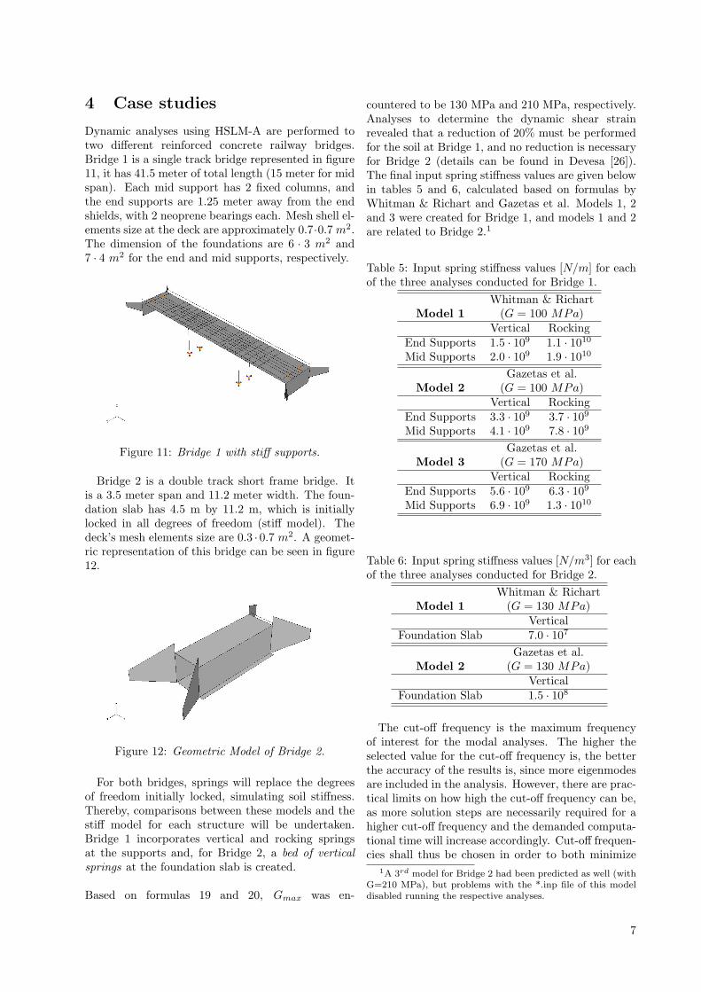
Dynamic analyses using HSLM-A are performed totwo different reinforced concrete railway bridges.Bridge 1 is a single track bridge represented in figure11, it has 41.5 meter of total length (15 meter for midspan). Each mid support has 2 fixed columns, andthe end supports are 1.25 meter away from the endshields, with 2 neoprene bearings each. Mesh shell el-ements size at the deck are approximately 0.7·0.7 m2.The dimension of the foundations are 6 · 3 m2 and7 · 4 m2 for the end and mid supports, respectively.

Figure 11: Bridge 1 with stiff supports.

Bridge 2 is a double track short frame bridge. Itis a 3.5 meter span and 11.2 meter width. The foun-dation slab has 4.5 m by 11.2 m, which is initiallylocked in all degrees of freedom (stiff model). Thedeck’s mesh elements size are 0.3 · 0.7 m2. A geomet-ric representation of this bridge can be seen in figure12.

Figure 12: Geometric Model of Bridge 2.

For both bridges, springs will replace the degreesof freedom initially locked, simulating soil stiffness.Thereby, comparisons between these models and thestiff model for each structure will be undertaken.Bridge 1 incorporates vertical and rocking springsat the supports and, for Bridge 2, a bed of verticalsprings at the foundation slab is created.

Based on formulas 19 and 20, Gmax was en-

countered to be 130 MPa and 210 MPa, respectively.Analyses to determine the dynamic shear strainrevealed that a reduction of 20% must be performedfor the soil at Bridge 1, and no reduction is necessaryfor Bridge 2 (details can be found in Devesa [26]).The final input spring stiffness values are given belowin tables 5 and 6, calculated based on formulas byWhitman & Richart and Gazetas et al. Models 1, 2and 3 were created for Bridge 1, and models 1 and 2are related to Bridge 2.1

Table 5: Input spring stiffness values [N/m] for eachof the three analyses conducted for Bridge 1.

Whitman & RichartModel 1 (G = 100 MPa)

Vertical RockingEnd Supports 1.5 · 109 1.1 · 1010

Mid Supports 2.0 · 109 1.9 · 1010

Gazetas et al.Model 2 (G = 100 MPa)

Vertical RockingEnd Supports 3.3 · 109 3.7 · 109

Mid Supports 4.1 · 109 7.8 · 109

Gazetas et al.Model 3 (G = 170 MPa)

Vertical RockingEnd Supports 5.6 · 109 6.3 · 109

Mid Supports 6.9 · 109 1.3 · 1010

Table 6: Input spring stiffness values [N/m3] for eachof the three analyses conducted for Bridge 2.

Whitman & RichartModel 1 (G = 130 MPa)

VerticalFoundation Slab 7.0 · 107

Gazetas et al.Model 2 (G = 130 MPa)

VerticalFoundation Slab 1.5 · 108

The cut-off frequency is the maximum frequencyof interest for the modal analyses. The higher theselected value for the cut-off frequency is, the betterthe accuracy of the results is, since more eigenmodesare included in the analysis. However, there are prac-tical limits on how high the cut-off frequency can be,as more solution steps are necessarily required for ahigher cut-off frequency and the demanded computa-tional time will increase accordingly. Cut-off frequen-cies shall thus be chosen in order to both minimize

1A 3rd model for Bridge 2 had been predicted as well (withG=210 MPa), but problems with the *.inp file of this modeldisabled running the respective analyses.

7

the analyses time and provide accurate and reliableresults. 30 Hz was chosen for both bridges, regard-ing accelerations and displacements analyses [27]. Inwhat concerns section forces, the most appropriatecut-off frequencies are 60 Hz and 160 Hz for Bridges 1and 2, respectively [28]. Moreover, to choose an accu-rate time increment (∆t) for the analysis is importantto ensure the correct response is captured. Based onequation 21 [21], 0.0033 s was used for accelerationsand displacements at both bridges, whilst for sectionforces 0.0017 s and 0.000625 s was adopted.

∆t ≤ Tmin10

=1

10 · fmax(21)

where fmax is the designated cut-off frequency.

The dynamic analyses are performed by succes-sively traveling HSLM-A1 to HSLM-A10 over thebridges, assuming velocities between 100 and 300km/h, with a speed interval of 5 km/h (2.5 km/haround resonance peaks). For the node where theabsolute highest acceleration was verified at each ofthe 4 models of Bridge 1, the graphics of speed plotsand time histories were given (figures 13 to 16):

Figure 13: Left) Maximum accelerations of node 189according to speed (Stiff model). Right) Time Historyof the same node at 170 km/h, with HSLM-A2.

Figure 14: Left) Maximum accelerations of node 187according to speed (Model 1). Right) Time History ofthe same node at 190 km/h, with HSLM-A4.

The accelerations at the stiff model vary between−2.62 m/s2 and 2.82 m/s2 (downwards and up-wards). On the other hand, the envelope for model

Figure 15: Left) Maximum accelerations of node 187according to speed (Model 2). Right) Time History ofthe same node at 247.5 km/h, with HSLM-A2.

Figure 16: Left) Maximum accelerations of node 187according to speed (Model 3). Right) Time History ofthe same node at 242.5 km/h, with HSLM-A4.

1 is −6.89 m/s2 and 6.31 m/s2. Model 2 respondedwith accelerations within the range −5.32 m/s2 to4.81 m/s2. Finally, model 3 had an accelerationinterval of −3.36 m/s2 to 3.28 m/s2. It is clearlyshown that models 1 and 2 are not in accordancewith the prescribed recommendations, exceeding theadmissible acceleration of 3.5 m/s2. Model 3 hasalso registered accelerations over the stiff model,enhancing the idea that soil modelling cannot beneglected.

The analysis conducted for the displacementsrevealed the speed plots and time histories for thenode with the highest value as shown in figures 17to 20.

Maximum downwards displacement were foundout to be very similar for all models in terms ofabsolute results, and in accordance to figure 6.Moreover, it is possible to estimate the compressionin soil based on speed plots (left figures): thedownwards and upwards values are mirrored below0, since the downwards values are higher. Therefore,that value corresponds to the compression in soildue to dynamic loads (admitting the stiff modeldisplacement values are exactly mirrored in ordinate0).

The section forces of interest in this paper are

8

Figure 17: Left) Maximum deflections of node 175according to speed (Stiff model). Right) Time Historyof the same node at 275 km/h, with HSLM-A7.

Figure 18: Left) Maximum deflections of node 499according to speed (Model 1). Right) Time History ofthe same node at 280 km/h, with HSLM-A9.

Figure 19: Left) Maximum deflections of node 499according to speed (Model 2). Right) Time History ofthe same node at 280 km/h, with HSLM-A7.

Figure 20: Left) Maximum deflections of node 175according to speed (Model 3). Right) Time History ofthe same node at 285 km/h, with HSLM-A7.

the shear force and bending moment over bridgedeck. Envelopes of the results for the HSLMs areshown in the same graphic to compare the differentmodels.

Figure 21: Shear forces along path for the 4 models -Bridge 1.

Figure 22: Bending moments along path for the 4models - Bridge 2.

The stiff model is not able to guarantee safe sideresults for the entire bridge, as it is possible toobserve in these graphics. For both shear force andbending moment, the extremities of the bridge arein prominence concerning dissimilar results. Model1 registers a shear force 300% higher than the stiffmodel at end supports, and 350% higher for thebending moment.

In pursuance of the type of results displayedfor Bridge 1, accelerations, displacements and sec-tion forces were analysed for Bridge 2. The speedplot and time history of the node with the highestacceleration for each model are presented below.

Stiff model accelerations vary from −0.016 m/s2

to 0.016 m/s2. Higher values were obtained withmodels 1 and 2: the first presented results inthe range −4.16 m/s2 to 4.29 m/s2, which arealready off the prescribed limits; the second repliedresults between −2.50 m/s2 and 2.91 m/s2. Theseextremely big differences to the stiff model arerelated to the absence of vertical modes of vibrationbelow the cut-off frequency in that model (30 Hz).

9

Figure 23: Left) Maximum accelerations of node 107according to speed (Stiff model). Right) Time Historyof the same node for speed 187.5 km/h, with HSLM-A2.

Figure 24: Left) Maximum accelerations of node 21according to speed (Model 1). Right) Time History ofthe same node for speed 300 km/h, with HSLM-A9.

Figure 25: Left) Maximum accelerations of node 401according to speed (Model 2). Right) Time History ofthe same node for speed 210 km/h, with HSLM-A9.

On another hand, both models 1 and 2 alreadyinclude vertical modes below 30 Hz with relevantparticipation mass, due to the loss of stiffness causedby the springs inclusion in the models. It is, thus,considered to be essential, not only the revisionof the cut-off frequency of 30 Hz established bythe Swedish Railway Authority [27], but also toinclude soil stiffness in the models, since it providesoff-recommended accelerations, not captured withthe stiff model.

The analyses undertaken for the displacementsat Bridge 2 caused by the dynamic loads repliedresults as shown in the next series of graphics.

Figure 26: Left) Maximum deflections of node 107according to speed (Stiff model). Right) Time Historyof the same node for speed 185 km/h, with HSLM-A2.

Figure 27: Left) Maximum deflections of node 404according to speed (Model 1). Right) Time History ofthe same node for speed 300 km/h, with HSLM-A1.

Figure 28: Left) Maximum deflections of node 18 ac-cording to speed (Model 2). Right) Time History ofthe same node for speed 100 km/h, with HSLM-A2.

Once again, due to the 30 Hz cut-off frequency,no vertical eigenmodes are present in the analysesundertaken for the stiff model, thereby the displace-ments are practically 0. Since models 1 and 2 includevertical eigenmodes, more realistic displacementvalues were obtained. Nevertheless, they are all incompliance with figure 6.

The comparisons of the three models, in whatconcerns shear force and bending moment, can beseen in the following graphics.

It is easily observed that models 1 and 2 replied,almost for the entire deck, higher values when com-paring to the stiff model, both on shear force and

10

Figure 29: Shear forces along path for the 3 models -Bridge 2.

Figure 30: Bending moments along path for the 3models - Bridge 2.

bending moment. The differences between modelsfor the shear force, over deck extremities, is not sig-nificant though. Higher dissimilarities are observedfor mid deck, where models with soil springs repliedvalues between 250% and 300% higher than the stiffmodel. Nevertheless, the biggest differences have oc-curred in the comparison of bending moment: deckextremities are more affected when looking at themodels with elastic foundation springs, with values ofnegative bending moment 200% higher than the stiffmodel, and with values of positive bending momentalmost reaching 700% higher than the stiff model.

5 Conclusions

The inclusion of springs in the model, in order tosimulate soil/structure interaction, has a very signif-icant influence in the eigenmodes and eigenfrequen-cies, which, at the end, are responsible for the differ-ences in the results;

Considering soil stiffness in the numerical analy-sis allows a reduction of the cut-off frequencies, whenstudying section forces. Since the overall stiffness ofthe structure decreases, a significant contribution ofthe effective mass (normally taken as > 90% of totalmass) is tangible with lower eigenfrequencies. There-fore, with a cut-off frequency reduction, the time of

the analysis decreases;30 Hz as cut-off frequency for accelerations and dis-

placements analyses seems to be extremely low forbridges similar with Bridge 2 when stiff supports areconsidered, since important vertical eigenmodes maybe excluded. Eurocode 1 [20] presents a different per-spective over choosing this limit, which seems indeedmore appropriate;

When taking soil stiffness into consideration, reso-nance can occur for a different train, different speedand different deck node when comparing to the cor-responding stiff model. Therefore, neither the sametrain nor the same speed can be used for differentmodels. Instead, a full analysis must be performedfor each model;

In what concerns soil stiffness inclusion, some mod-els were not in compliance with the limit state pro-posed in Eurocode 1 [20], regarding vertical accel-erations, whilst others provided admissible values.But for all models, such values were increased signif-icantly: for Bridge 1, while model 1 and 2 providedoff-limit values, model 3 gave values quite close fromthe recommendation - 3.5m/s2; as for Bridge 2, ac-celerations were extremely increased by the time ofsoil inclusion. The appearance of important verti-cal eigenmodes below 30 Hz was the main reason forsuch event. Even though model 2 of that bridge pre-sented tolerable values, this phenomena should notbe neglected;

Maximum displacements values were not affectedby the dynamic analyses undertaken in the differentmodels.

Section forces can increase in some parts of thedeck bridges and decrease in some other parts, whensoil is included in the model. Although no guaranteescan be given for all types of bridges, it can happenwith two very different structures, as it was provedin chapter 4. Shear forces and bending moments areclearly increased in deck ends if soil stiffness is in-cluded in the model;

It is considered to be of great importance the soilconsideration in the numerical model of a bridge, inparticular when studying accelerations and sectionforces. Ideally, two models should be adopted, onestiff and another with soil stiffness. Subsequently, anenvelope of the two results should be done.

6 Acknowledgements

The author wishes to acknowledge Scanscot Technol-ogy AB, located in Lund, Sweden, not only for all thesupport and interest in this work, but also for thekindness and friendship he was treated with. Also,to his home University, Instituto Superior Tecnico,in Lisboa, where he studied 5 years of his life, miss-ing it already.

11

References

[1] XIX Cimeira Luso-Espanhola, Figueira da Foz,November 2003.

[2] Willis, R. Appendix to the report of the commis-sioners appointed to inquire into the applicationof iron to railway structures. Stationery Office,London, 1849.

[3] Timoshenko, S. P. Vibration Problems in En-gineering. Van Nostrand Company, New York,1928.

[4] Jeffcott, H. H. On the vibrations of beams underthe action of moving loads. Philosophical Maga-zine, Series 7,8:66–97, 1929.

[5] Stanisic, M. M. and Hardin, J. C. On the re-sponse of beams to an arbitrary number of con-centrated moving masses. Journal of FranklinInstitute, 287:66–97, 1969.

[6] Inglis, C. E. A Mathematical Teatrise on Vibra-tions in Railway Bridges. Cambridge UniversityPress, 1934.

[7] Fryba, L. Vibration of Solids and Structures un-der Moving Loads. Thomas Telford, 3rd edition,1999.

[8] Fryba, L. A rough assessment of railway bridgesfor high speed trains. Elsevier Science Ltd. En-gineering Structures, 23:548–556, 2001.

[9] Yang, Y. B.; Yau, J. D.; Wu, W. S. Vehicle-Bridge Interaction Dynamics: With Applica-tions to High-Speed Railways. World ScientificPublishing Co. Pte. Ltd., Singapore, 2004.

[10] Xia, H.; De Roeck, G.; Zhang, N.; Maeck, J.Experimental analysis of a high-speed railwaybridge under thalys trains. Academic Press.Journal of Sound and Vibration, 268:103–113,2003.

[11] Xia, H.; Zhang, N.; De Roeck, G. Dynamic anal-ysis of high speed railway bridge under articu-lated trains. Elsevier Ltd. Computers & Struc-tures, 81:2467–2478, July 2003.

[12] Castillo, Felipe Galbadon; Ruigomez, Jose Ma

Goicolea. Calculo dinamico de un viaducto deseccion mixta hormigon-acero sometido a ac-ciones de trenes de alta velocidad. Technical re-port, E.T.S. Enginieros de Caminos, Canales yPuertos, Madrid, 2005. (in Spanish).

[13] Moreno Delgado, R.; Santos, S. M. Modelling ofrailway bridge-vehicle interaction on high-speedtracks. Computers & Structures, 63(3):511–523,1997.

[14] Barkan, D. D. Dynamics of Bases and Founda-tions. McGraw-Hill Book Company, Inc., 1962.

[15] Krylov, V. V. Generation of ground vibrationsby superfast trains. Applied Acoustics, 44:149–164, 1995.

[16] Degrande, G. and Schillemans, L. Free field vi-brations during the passage of a thalys high-speed train at variable speed. Journal of Soundand Vibration, 247(1):131–144, 2001.

[17] Auersch, L. The excitation of ground vibrationby rail traffic: theory of vehicle-track-soil inter-action and measurements on high-speed lines.Journal of Sound and Vibration, 284:103–132,2005.

[18] Galvın, P.; Domınguez, J. High speed train in-duced ground motion and interaction with struc-tures. Journal of Sound and Vibration, 307:755–777, 2007.

[19] Lombaert, G.; Degrande, G.; Vanhauwere, B.;Vandeborght, B.; Francois, S. The control ofground borne vibrations from railway traffic bymeans of continuous floating slabs. Journal ofSound and Vibration, 297:946–961, 2006.

[20] CEN - Comite Europeen de Normalisation. Eu-rocode 1: Actions on structures - Part 2: Trafficloads on bridges, EN1991-2, July 2002.

[21] ERRI Committee D214. Rail Bridges for Speeds> 200 km/h, RP 9, Part A: Synthesis of theresults of D214 research; Part B: Proposed UICLeaflet. Technical report, UIC, December 1999.

[22] CEN - Comite Europeen de Normalisa-tion. Eurocode - Basis of Structural Design,EN1990:2002/A1, December 2005.

[23] Whitman, R. V.; Richart, F. E. Design proce-dures for dynamically loaded foundations. TheUniversity of Michigan, Industry Program of theCollege of Engineering, February 1967.

[24] Mylonakis, G.; Gazetas, G.; Nikolaou, S. andChauncey, A. Development of analysis and de-sign procedures for spread footings. Technical re-port, MCEER, University at Buffalo, State Uni-versity of New York, Department of Civil, Struc-tural and Environmental Engineering, October2002.

[25] Banverket. Jorddynamiska analyser. Technicalreport, BVF, September 2001. (in Swedish).

[26] Devesa, Joao Ricardo. Influence of soil stiffnesson the dynamic behaviour of bridges traffickedby high speed trains. MSc Thesis, Insituto Su-perior Tecnico, Lisboa, September 2008.

12

[27] BVS 583.10 Broregler for nybyggnad - BV Bro,Utgava 9, 2006. (in Swedish).

[28] Lundin, Bjorn; Martensson, Philip. Finding gen-eral guidelines for choosing appropriate cut-offfrequencies for modal analyses of railway bridgestrafficked by high-speed trains. Master’s disser-tation, Lund University, Division of Solid Me-chanics, 2006.

13