Inflation and the Dispersion of Real Wages

Alok KumarDepartment of Economics

University of VictoriaVictoria, British Columbia

Canada, V8W 2Y2Email: kumara@uvic.ca

October, 2003

Abstract

The effects of inflation on real wage dispersion and welfare are studied in a cash-in-advance economywith a Walrasian goods market but a labor market with search friction. In the labor market,firms post wages and both employed and unemployed workers search among the posted wages. Inequilibrium, a higher inflation rate reduces the dispersion in real wages. This result is consistentwith both the observed trends in wage dispersion and the inflation rate witnessed in the 1980’sand the 1990’s in the U.S. and the empirical literature linking reduced inflation to greater wagedispersion. While higher inflation always lowers consumption, output, and employment, the optimalinflation rate exceeds the Friedman rule.

Key Words: Inflation, Wage Posting, Search, Dispersion of Real WagesJEL Code: E0, E5, N3

I thank Michelle Alexopoulos, Charles Beach, Allen Head, Hiroyuki Kasahara, Huw Lloyd-Ellis, SumonMazumdar, Shouyong Shi, Gregor Smith, and participants of the Canadian Economic Association meeting2002, the Macro workshop at Queen’s University, Kingston, and Mid-West Macro Meeting 2003 for theirhelpful comments.

1. Introduction

In the eighties and the nineties, wage dispersion, including residual wage dispersion (i.e. differ-

ences in wages among workers with similar skills and job characteristics) increased dramatically in

the U.S. (OECD (1997), Katz and Autor (1999)). Over this period the inflation rate also declined

significantly relative to what it had been the 1970’s. In this paper a general equilibrium monetary

model is developed in which lower expected inflation increases the dispersion in real wages. This

finding is consistent not only with the observed trends in wage dispersion and expected inflation

for the U.S., but also with a sizeable empirical literature linking reduced inflation to greater wage

dispersion for several different countries and time periods.

Lipsey and Swedenborg (1999) study the relationship between the price levels and wage dis-

persion for fifteen OECD countries for the period 1979-90. They find that the price level is neg-

atively related to wage dispersion. Erikson and Ichino (1995) examine the effect of inflation on

wage earnings differentials over the period 1976-90 in Italy using the wage data taken from metal-

manufacturing firms. They find that a higher inflation rate significantly reduced changes in wage

earnings differentials. Hammermesh (1986) analyzes the relationship between the inflation rate

and the dispersion in the relative wage changes for the period 1955-81 in the United States us-

ing data from twenty two-digit manufacturing industries and finds that higher inflation, especially

unexpected inflation, reduced the dispersion in the relative wage changes.1

These empirical findings are at variance with the predictions of the models which assume that

firms face costs or other barriers to changing nominal wages. Inflation allows firms facing negative

demand shocks to bring real wages in line with productivity (Tobin 1972). In the case of downward

nominal rigidity, inflation increases real wage dispersion by allowing firms to provide real rewards

to those whose productivity is increasing, while cutting rewards to those who are becoming less

productive without reducing the nominal wages (Hammermesh 1986). Akerlof, Dickens, and Perry

(1996) argue that inflation enables the firms facing downward nominal wage rigidity to change real

wages in the case of negative demand shocks.2

1 Allen (1987) studies the relative wage variability across industries in the U.S. and finds that both expectedand unexpected inflation has negative though insignificant effect on the relative wage variability for theperiod 1947-83. Souza (2002) examines the changes in wage dispersion of male workers in metropolitanareas of Brazil for the period 1981-97 and finds that higher expected inflation rate reduced the standarddeviation of log of wages, though increased the ratio of 90th to 10th percentile .

2 Drazen and Hammermesh (1987) develop a model in which agents are confused between the aggregateand the relative shocks and the degree of indexation of wages depends on the uncertainty about inflation.

1

Many models with nominal rigidities imply that firms will follow a strategy of the [s,S] variety

when setting wages (e.g. Sheshinski and Weiss (1977), Benabou (1988, 1992) , Diamond (1993)).3

In such models, a reduction in the trend inflation rate reduces the bound of real wages within which

wages are not changed. That is, lower inflation reduces the range in which nominal wages do not

respond to price level changes, resulting in less dispersion of real wages rather than more.

In our model, the goods market is Walrasian with purchases subject to a standard cash-

in-advance constraint. The labor market is characterized by search frictions, with workers and

firms brought together by a matching function. Wages are determined in a general equilibrium

variant of the model developed by Burdett and Mortensen (1998), in which firms post wages

and both employed and unemployed workers search. By assumption, workers cannot direct their

search towards higher or lower wage offers (undirected search). In this framework, on-the-job

search weakens the market power of wage-posting firms, and thus wage dispersion is an equilibrium

outcome even if firms and workers are both ex ante homogeneous. Variants of this model have been

extensively used to explain wage dispersion (e.g. Bontemps, Robin, and van den Berg (2000), van

den Berg and Ridder (1998), Vurren, van den Berg, and Ridder (2000)).

In the model studied, higher expected inflation, by eroding the expected future value of fiat

money, reduces the profitability of firms. In addition, the real reservation wage of unemployed

workers rises, which further lowers the profitability of firms inducing them to post a smaller number

of vacancies.

The higher real reservation wage of unemployed workers increases the lower support of the real

wage earnings distribution. The effect of inflation on the upper support, however, is mitigated by

two factors. Firstly, firms posting the highest real wage do not face any competition from other

firms to retain their workers, while firms posting lower real wages do. The result is that the firms

posting the highest real wage need not increase their real wage as much as the firms posting the

lowest real wage. Secondly, the decline in the level of vacancies posted reduces the effectiveness of

In such a set-up, if the degree of indexation is constant, higher unanticipated inflation increases thevariance of relative wage changes. However, if the degree of indexation increases with unanticipatedinflation, then the variance of relative wage changes may decline with unanticipated inflation. They findthat unexpected inflation significantly reduced the relative wage dispersion in Israel during the period1956-82. Expected inflation has negative though insignificant effect. In contrast to this model, in ourmodel there is no confusion between the aggregate and the relative shocks and the degree of indexationis constant.

3 In these models, firms post prices and incur menu cost in changing them. The results of these modelsremain the same if we assume that firms post wages and face menu cost in changing them.

2

on-the-job search in weakening the market power of firms by lowering the matching rate of workers.

Consequently, the support of the distribution of real wage earnings declines and the dispersion

measured by the coefficient of variation and the ratio of 90th percentile to 10th percentile of the

distribution of real wage earnings are reduced. In addition, a fall in the level of vacancies reduces

employment and output.

The result that inflation affects the real reservation wage of unemployed workers has an in-

teresting welfare implication, that the optimal rate of inflation exceeds the Friedman rule. The

economy considered in this paper has two sources of inefficiency: i) the buyers’ nominal money

balance constraint and ii) the undirected search by workers. The Friedman rule removes the first

source of inefficiency. But, as the inflation rate approaches the Friedman rule, the real reservation

wage of the unemployed workers falls for a given level of consumption, and firms create too many

vacancies relative to the social optimum.

There is sizeable empirical literature linking lower real minimum wage with larger wage dis-

persion (DiNardo, Fortin, Lemieux 1996, Katz and Autor 1999, Lee 1999). For example, DiNardo

et.al. (1996) and Lee (1999) find that the increased wage dispersion in the eighties in the U.S. is

largely due to the decline in the federal minimum wage in real terms. Lee (1999) also suggests that

the changes in the minimum wage has sizeable “spill-over” effect i.e., it affects the distribution of

wages above the minimum wage.

In this paper, we also consider the effect of changes in the binding real minimum wages (i.e.

real minimum wage higher than the real reservation wage of the unemployed workers) on the

distribution of real wage earnings. We find that lower real minimum wage increases the dispersion

of real wages and does so by affecting the entire distribution. In addition, for a given real minimum

wage higher inflation rate reduces the dispersion in real wages, though its effect on the dispersion

is smaller compared to the case in which the real minimum wage is not binding.

The rest of the paper is organized as follows. Section 2 describes the model. In Section 3, the

optimal strategies of households are characterized. Section 4 defines a class of stationary monetary

equilibrium and derives conditions for the existence of a unique stationary monetary equilibrium

with non-degenerate real wage earnings distribution. Section 5 studies the effect of inflation on

output and welfare in equilibrium. In Section 6, an example is constructed to illustrate the welfare

cost of inflation. In Section 7, the effect of inflation rate on real wage dispersion is analyzed. Section

8 examines the robustness of the result that higher inflation reduces real wage dispersion. Section

9 examines the effect of real minimum wage on the dispersion of real wages. Section 10 concludes

and summarizes. All the proofs are contained in Appendix 1.

3

2. The Economy

2.1 The Household Structure

Consider a cash-in-advance economy with no aggregate uncertainty comprised of a large num-

ber of infinitely-lived identical households with measure one. Each household, in turn, is comprised

of three types of infinitely-lived members: a buyer, a firm, and a unit measure of identical workers.4

Time is discrete.

Each type of member in the household plays a distinct role. The buyer buys the household’s

desired consumption goods in the goods market. The firm posts vacancies, hires workers in the

labor market, produces, and sells goods in the goods market. Unemployed workers search for

suitable jobs. Employed workers work and also search for better jobs. It is assumed that the firm

uses a linear production technology, and each employee produces y units of goods.

Members of the household do not have independent preferences. Rather, the household pre-

scribes the trading and production strategies for each member to maximize overall household utility.

The members of the household share equally in the utility generated by the household consumption.

The household maximizes the discounted sum of utilities from the sequence of consumption less

the disutility arising from the workers’ working and searching and posting of vacancies by the firm.

The household’s inter-temporal utility is represented by

U =∞∑

t=0

1(1 + r)t

[u(ct)− (1 + φ)et − ut − k(vt)

](2.1)

where r is the rate of time-preference, and u(ct) and k(vt) are the utility derived from consumption

ct and the disutility of posting vt level of vacancies respectively. φ is the disutility of working. et

and ut are respective measures of employed and unemployed workers. For simplicity, it is assumed

that the disutility of search is unity for both employed and unemployed workers.5 Let u′(ct) > 0

4 The firm need not be the part of the household. One can assume that firms are owned by the householdsand firms take decisions in order to maximize the utility of the owners and rebate their profits equallyto the owners. The construction of the household is similar to that in Fuerst (1992), Merz (1995), Shi(1999), and Head and Shi (2000). This construction makes the model highly tractable analytically.

5 With different disutility of search for employed and unemployed workers, the real reservation wage ofunemployed workers depends not only on the disutility of work but also on the expected gain fromsearch, which makes the model analytically complex (Kumar 2003). One can also endogenize the search-intensities of employed and unemployed workers. Endogenization of search-intensity will lead to consider-able analytical and computational complexity. The reason is that the model generates a non-degeneratewage earnings distribution, which will induce non-degenerate distribution of search intensities, which is a

4

and u′′(ct) ≤ 0. Also, let k(vt) be strictly increasing and convex and satisfy limvt→0 vtk′(vt) = 0,

and limvt→0 vtk′′(vt) + k′(vt) < ∞.

Trade in this economy takes place in two separate markets – the goods market and the labor

market. Since the focus of this paper is on the effects of inflation, it is assumed that buyers

require cash in order to buy goods, and firms pay wages in cash to workers. In order to facilitate

transactions, it is assumed that each household is endowed with M0 units of fiat money at time

zero. At the beginning of each subsequent period, each household receives (g − 1)Mt−1 units of

fiat money from the government as a lump-sum transfer, where Mt is the per-household aggregate

holding of fiat money at time t in the economy. The government plays no role in the economy,

other than making lump-sum transfers to the households. Households also acquire fiat money by

selling goods and from wage receipts of employed workers.

2.2 Goods Market

The goods market is assumed to be competitive. Let Mt be the post-transfer nominal money

balances with the representative household at the beginning of period t. The household allocates

the available money Mt to the buyer who goes to the goods market to acquire the consumption

goods subject to the cash-in-advance constraint

ptct ≤ Mt ∀ t (2.2)

where pt is the price of consumption goods and ct is the amount purchased. The firm produces

consumption goods using the existing employees and sells the goods in the goods market. The total

receipt of nominal money to the firm at time t is yptJt, where Jt is the total measure of employees

of the firm at time t.

2.3 Labor Market

The labor market is characterized by search frictions. Matches between workers and firms are

not instantaneous. Rather, firms who want to hire workers and workers who either want to work

or change their jobs have to search for suitable matches. Workers and firms are brought together

randomly through a matching function.

high dimensional object on which the wage posting strategies of firms must depend. Section 8.2 discussesthe likely effects of inflation when search-intensity is endogenous.

5

The process of wage determination is modeled using a version of the wage-posting model

developed by Mortensen (2000), which extends the wage-posting model of Burdett and Mortensen

(1998) by endogenizing the job arrival rates which are exogenous in the Burdett-Mortensen model.6

It is assumed that firms post wage offers. A posted wage offer is defined as a wage contract, which

fully specifies the nominal wages payable to the workers for all time to come. Workers (both

employed and unemployed) search among the posted wage offers.

Because of random matching, individual firms and workers face uncertainty in the match-

ing outcomes. In particular, random matching induces a non-degenerate distribution of money

holdings. As well, the model generates non-degenerate wage earnings distribution, which also in-

duces a non-degenerate distribution of money holdings. The construct of a large household makes

the distribution of money holding degenerate within the households and allows the analysis of a

representative household, which makes the model highly tractable analytically.

The representative household chooses the level of vacancies, the distribution of wage offers to

be posted (which can be degenerate), and the optimal job-acceptance strategies of both employed

and unemployed workers. For simplicity, we abstract from nominal rigidities and assume that a

wage offer promises to pay a constant real wage i.e., a real wage offer 7

w ≡

wt

pt,wt+1

pt+1, ....

≡ w, w, ..... (2.3)

where wt is the nominal wage at time t. In other words, the household offers fully-indexed wage con-

tracts to the searching workers. In addition, we assume that there is no possibility of renegotiation

as in Burdett and Mortensen (1998) and Mortensen (2000).8

In the model, the employed workers of the household, the employees of the firm, and the posted

vacancies can be heterogeneous with respect to real wages. Table 1 lists the notations of the workers

6 Rosholm and Svarer (2000) estimate the Mortensen (2000) model with firm-specific training expendituresusing the Danish labor market data, and find that the model provides a good characterization of someempirical features of the labor market.

7 One can assume that the households post infinite sequences of nominal wages to which they can crediblycommit and then restrict attention to a stationary equilibrium, which supports constant real wage offers.However, the assumption that households post constant real wage offers simplifies the exposition a greatdeal without affecting the results.

8 Section 8 below discusses extensions of the model, which allow for renegotiation similar to Coles (2001)and Postel-Vinay and Robin (2002). The qualitative results do not change.

6

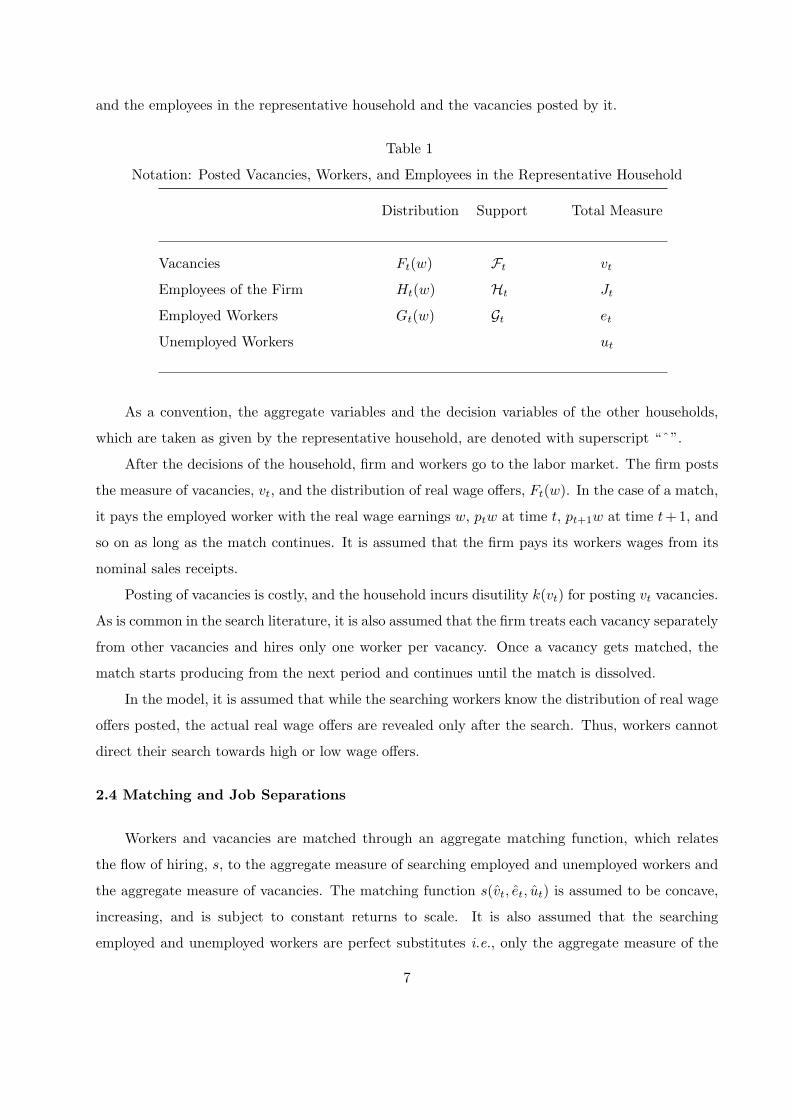
and the employees in the representative household and the vacancies posted by it.

Table 1

Notation: Posted Vacancies, Workers, and Employees in the Representative Household

Distribution Support Total Measure

Vacancies Ft(w) Ft vt

Employees of the Firm Ht(w) Ht Jt

Employed Workers Gt(w) Gt et

Unemployed Workers ut

As a convention, the aggregate variables and the decision variables of the other households,

which are taken as given by the representative household, are denoted with superscript “ˆ”.

After the decisions of the household, firm and workers go to the labor market. The firm posts

the measure of vacancies, vt, and the distribution of real wage offers, Ft(w). In the case of a match,

it pays the employed worker with the real wage earnings w, ptw at time t, pt+1w at time t+1, and

so on as long as the match continues. It is assumed that the firm pays its workers wages from its

nominal sales receipts.

Posting of vacancies is costly, and the household incurs disutility k(vt) for posting vt vacancies.

As is common in the search literature, it is also assumed that the firm treats each vacancy separately

from other vacancies and hires only one worker per vacancy. Once a vacancy gets matched, the

match starts producing from the next period and continues until the match is dissolved.

In the model, it is assumed that while the searching workers know the distribution of real wage

offers posted, the actual real wage offers are revealed only after the search. Thus, workers cannot

direct their search towards high or low wage offers.

2.4 Matching and Job Separations

Workers and vacancies are matched through an aggregate matching function, which relates

the flow of hiring, s, to the aggregate measure of searching employed and unemployed workers and

the aggregate measure of vacancies. The matching function s(vt, et, ut) is assumed to be concave,

increasing, and is subject to constant returns to scale. It is also assumed that the searching

employed and unemployed workers are perfect substitutes i.e., only the aggregate measure of the

7

workers searching matters and not their composition. The aggregate flow of matches then is given

by

s(vt, et, ut) = s(vt, 1) = s(vt) (2.4)

Since the aggregate measure of the workers in the economy is unity, (2.4) also defines the

aggregate matching rate of the workers. The aggregate matching rate of vacancies is given by

s(vt)vt

(2.5)

Assume that limvt→0 s(vt) → 0, limvt→0 s′(vt) →∞, and the aggregate matching rate of vacancies

is decreasing in the level of vacancies, vt.

Employed workers face the risk of unemployment. Each period fraction ρ of the household’s

existing matches are exogenously dissolved, with all such matches equally likely to fall in this group.

Note that matches dissolve for two reasons: i) employed worker in a match receives a better job

offer and ii) the match is dissolved exogenously. Only in the second case, an employed worker

becomes unemployed.

3. The Household’s Choice Problem

3.1 Timing

The representative household at the beginning of period t enters with the measures of unem-

ployed workers, ut, employed workers, et, employees of the firm, Jt, and their distribution over

real wage earnings. As previously mentioned, at the start of each period, the household receives a

lump-sum money transfer, which is added to the nominal money balances carried from the previous

period.

It is assumed that during any period t, trading takes place first in the goods market and

then in the labor market.9 The household gives the available money balance, Mt, to the buyer.

The firm produces consumption goods using the existing employees. Buyers and firms trade in

the goods market. After trading in the goods market, the buyer comes back to the household

9 The results of the model do not hinge on whether the goods market opens first or the labor market. Whatis important is that there be time separation between the time when the households receive money andwhen they spend it. For the inflation rate (which is the focus here) to have impact, the time-separationbetween the acquisition of money and spending is essential.

8

with the purchased goods and any residual nominal money balances and the firm with its nominal

sales receipts. The firm pays wages to its employees and the employees return to their respective

households with their nominal wage receipts. The profit of the firm, the wage receipts of employed

workers, and any residual money balance brought back by the buyer are added to the household

nominal money balance for the next period.

After trading in the goods market, the labor market opens up. The household decides the

measure of vacancies, vt, and the distribution of real wage offers, Ft(w), and prescribes the job-

acceptance strategies to workers. Workers search among the posted real wage offers and accept or

reject the offers received according to the prescribed job-acceptance strategies. Match dissolution

takes place. Trading in the labor market and exogenous dissolution of matches determine the next

period’s measure of employed workers, et+1, and their distribution over real wage earnings, the

measure of unemployed workers, ut+1, and the measure of employees of the firm, Jt+1, and their

distribution over real wages. At the end of the labor market session, workers and firms go back to

their respective households and consumption takes place. Time moves to the next period t + 1.

3.2 The Optimal Job Acceptance Strategies of Workers

Before formally setting the household optimization problem, it is convenient to discuss the op-

timal job-acceptance strategies of workers prescribed by the household. In the current environment,

the household knows that in any period t fraction ρ of the employed workers becomes unemployed

and fraction s(vt) receives new real wage offers, which they can accept or reject. Similarly, fraction

s(vt) of the unemployed workers realizes real wage offers, which they can accept or reject. The

following lemma characterizes the real reservation wages of employed and unemployed workers.

Lemma 1:

The job acceptance strategies prescribed by the household have a reservation property.

1. The real reservation wage of an employed worker is the real wage he currently earns.

2. The real reservation wage of an unemployed worker, w, satisfies

ωMt+1pt+1w = φ (3.1)

where ωMt+1 is the marginal value of nominal money balances to the household at time t + 1.

Intuitively, the contribution of employed workers earning higher real wages to the current

utility of the household is higher compared to employed workers earning lower real wages. At the

9

same time, in the next period all employed workers face the same aggregate matching rate, s(vt+1),

as well as the aggregate distribution of real wage offers, Ft+1(w). Therefore, it is optimal for the

household to instruct employed workers to accept any new real wage offer higher than their current

real wage. (3.1) equates the utility of working at the real reservation wage of unemployed workers

w (the left hand side) to the disutility of working (the right hand side). Thus it is optimal for the

household to instruct unemployed workers to accept any real wage offer w ≥ w.

3.3 The Household Optimization Problem

Taking the aggregate distribution of real wage offers, Ft(w), the aggregate distribution of real

wage earnings, Gt(w), the aggregate level of vacancies, vt, the price level in the goods market,

pt, the optimal choices of other households, the job-acceptance strategies of workers specified in

Lemma 1, and the initial conditionsM0, e0, u0, G0(w)

as given, the household chooses the

sequencect, Mt+1, vt, Ft(w)

∀ t ≥ 0 to solve the following problem.

10

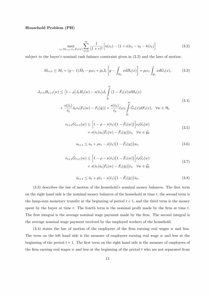
Household Problem (PH)

maxct,Mt+1,vt,Ft(w)

∞∑t=0

1(1 + r)t

[u(ct)− (1 + φ)et − ut − k(vt)

](3.2)

subject to the buyer’s nominal cash balance constraint given in (2.2) and the laws of motion:

Mt+1 ≤ Mt + (g − 1)Mt − ptct + ptJt

[y −

∫

Ht

xdHt(x)]

+ ptet

∫

Gt

xdGt(x), (3.3)

Jt+1Ht+1(w) ≤ [1− ρ

]JtHt(w)− s(vt)Jt

w∫

w

(1− Ft(x))dHt(x)

+s(vt)vt

utvt[Ft(w)− Ft(w)] +s(vt)vt

etvt

w∫

w

Gt(x)dFt(x), ∀w ∈ Ht

(3.4)

et+1Gt+1(w) ≤[1− ρ− s(vt)

(1− Ft(w)

)]etGt(w)

+ s(vt)ut[Ft(w)− Ft(w)]vt, ∀w ∈ Gt

(3.5)

ut+1 ≤ ut + ρet − s(vt)(1− Ft(w)

)ut, (3.6)

et+1Gt+1(w) ≤[1− ρ− s(vt)

(1− Ft(w)

)]etGt(w)

+ s(vt)ut[Ft(w)− Ft(w)]vt, ∀w ∈ Gt

(3.7)

ut+1 ≤ ut + ρet − s(vt)(1− Ft(w)

)ut, (3.8)

(3.3) describes the law of motion of the household’s nominal money balances. The first term

on the right hand side is the nominal money balances of the household at time t, the second term is

the lump-sum monetary transfer at the beginning of period t + 1, and the third term is the money

spent by the buyer at time t. The fourth term is the nominal profit made by the firm at time t.

The first integral is the average nominal wage payment made by the firm. The second integral is

the average nominal wage payment received by the employed workers of the household.

(3.4) states the law of motion of the employees of the firm earning real wages w and less.

The term on the left hand side is the measure of employees earning real wage w and less at the

beginning of the period t + 1. The first term on the right hand side is the measure of employees of

the firm earning real wages w and less at the beginning of the period t who are not separated from

11

their matches exogenously. The second term is the measure of employees who leave their matches

because they receive higher real wage offers. The third and fourth terms together give the measure

of new matches formed on the vacancies posted with real wage offers of w and less.

(3.5) specifies the law of motion of the employed workers of the household with real wage

earnings of w and less. The term on the left hand side is the measure of employed workers with the

real wage earnings of w and less at the beginning of period t + 1. The first term on the right hand

side is the measure of employed workers with real wage earnings of w and less at the beginning of

the period t who remain in the same pool at the end of the period. An employed worker leaves this

pool either due to exogenous dissolution of match or because he receives a real wage offer higher

than w. The second term is the measure of unemployed workers who receive the real wage offers

of w and less.

(3.6) describes the law of motion of unemployed workers. The first term on the right hand

side is the measure of unemployed workers in the household at the beginning of time t. The second

term is the measure of employed workers who become unemployed due to exogenous dissolutions

at time t. The third term is the measure of unemployed workers at time t who become employed.

(3.7) and (3.8) are the aggregate laws of motion of employed workers earning real wages w and

less and unemployed workers respectively. They have interpretation similar to (3.5) and (3.6).

3.4 The Optimal Choice of ct and Mt+1

Let ωct and ωMt be the Langrangian multipliers associated with the constraints (2.2)and (3.3)

respectively. The first order conditions for the optimal choices of ct and Mt+1 are given by

ct :u′(ct)

pt= ωct + ωMt, (3.9)

Mt+1 : ωMt =1

1 + r[ωMt+1 + ωct+1]. (3.10)

The slackness condition associated with the optimal choice of consumption is given by

ωct[Mt − ptct] = 0. (3.11)

The sufficient condition for the buyer’s nominal cash balance constraint to be binding is that

the nominal interest rate be strictly positive

(1 + r)u′(ct)pt+1

u′(ct+1)pt− 1 > 0 (3.12)

12

We will assume that the buyer’s nominal cash balance constraint is binding for the rest of

the paper. The first order conditions have the usual interpretations. For the optimal choice of

consumption, the household equates the marginal benefit of spending one unit of money (the left

hand side of (3.9)) with the marginal cost (the right hand side of (3.9)), which is the sum total of

the Langrangian multipliers associated with the buyer’s nominal cash balance constraint and the

law of motion of nominal money holding.

(3.10) states that by not spending one unit of money in the current period, the household

relaxes the buyer’s nominal cash balance constraint and the constraint on the household nominal

money balance next period. (3.9) and (3.10) together imply that the marginal value of nominal

money balances, ωMt, is given by

ωMt =1

1 + r

u′(ct+1)pt+1

. (3.13)

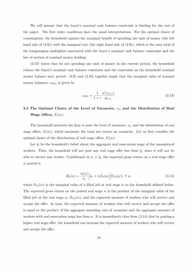
3.5 The Optimal Choice of the Level of Vacancies, vt, and the Distribution of Real

Wage Offers, Ft(w)

The household instructs the firm to post the level of vacancies, vt, and the distribution of real

wage offers, Ft(w), which maximize the total net return on vacancies. Let us first consider the

optimal choice of the distribution of real wage offers, Ft(w).

Let w be the household’s belief about the aggregate real reservation wage of the unemployed

workers. Then, the household will not post any real wage offer less than w, since it will not be

able to attract any worker. Conditional on w ≥ w, the expected gross return on a real wage offer

w posted is

Rt(w) =s(vt)vt

[ut + etGt(w)

]ΩJt(w), ∀ w. (3.14)

where ΩJt(w) is the marginal value of a filled job at real wage w to the household defined below.

The expected gross return on the posted real wage w is the product of the marginal value of the

filled job at the real wage w, ΩJt(w), and the expected measure of workers who will receive and

accept the offer. In turn, the expected measure of workers who will receive and accept the offer

is equal to the product of the aggregate matching rate of vacancies and the aggregate measure of

workers with real reservation wage less than w. It is immediately clear from (3.14) that by posting a

higher real wage offer, the household can increase the expected measure of workers who will receive

and accept the offer .

13

The marginal value of a filled job with the real wage w can be defined recursively as

ΩJt(w) =1

1 + r

[pt+1(y − w)ωMt+1

[1− ρ− s(vt+1)(1− Ft+1(w))

]ΩJt+1(w)

] (3.15)

The first term on the right hand side is the flow value of profit evaluated using the marginal

value of nominal money balances at time t+1. The second term is the expected continuation value

of the match. The term reflects the fact that the match can dissolve either exogenously or due to

the employed worker leaving the match for a better offer. It also shows that the employed workers’

turnover is lower at higher real wages.

The household will post real wage offer such that

w ∈ argmaxw

Rt(w) ≡ R∗t . (3.16)

Let w∗ be an optimal real wage offer. Then, the household will post real wage offers other

than w∗ if and only if all the other posted real wage offers give return equal to R∗t . Utilizing (3.16),

one can express the total net return on posted vacancies as

TRt ≡ −k(vt) + R∗t vt. (3.17)

Then, the optimal choice of the measure of vacancies, vt, satisfies the following first order

condition

k′(vt) =s(vt)vt

[ut + etGt(w∗)

]ΩJt(w∗). (3.18)

(3.18) equates the marginal cost of posting a vacancy to the expected marginal benefits. Also

at the optimal choice of vacancies, it must be the case that TRt ≥ 0.

14

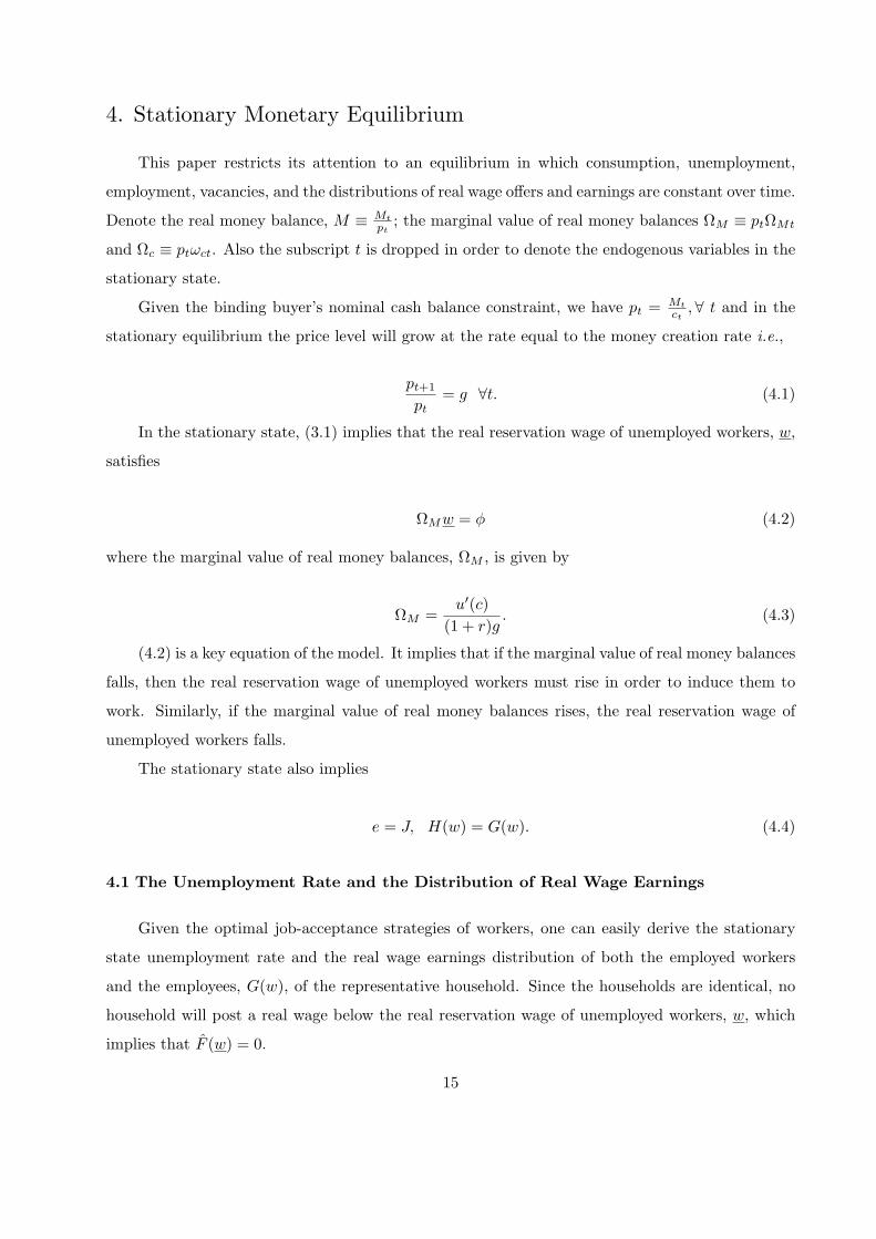
4. Stationary Monetary Equilibrium

This paper restricts its attention to an equilibrium in which consumption, unemployment,

employment, vacancies, and the distributions of real wage offers and earnings are constant over time.

Denote the real money balance, M ≡ Mt

pt; the marginal value of real money balances ΩM ≡ ptΩMt

and Ωc ≡ ptωct. Also the subscript t is dropped in order to denote the endogenous variables in the

stationary state.

Given the binding buyer’s nominal cash balance constraint, we have pt = Mt

ct, ∀ t and in the

stationary equilibrium the price level will grow at the rate equal to the money creation rate i.e.,

pt+1

pt= g ∀t. (4.1)

In the stationary state, (3.1) implies that the real reservation wage of unemployed workers, w,

satisfies

ΩMw = φ (4.2)

where the marginal value of real money balances, ΩM , is given by

ΩM =u′(c)

(1 + r)g. (4.3)

(4.2) is a key equation of the model. It implies that if the marginal value of real money balances

falls, then the real reservation wage of unemployed workers must rise in order to induce them to

work. Similarly, if the marginal value of real money balances rises, the real reservation wage of

unemployed workers falls.

The stationary state also implies

e = J, H(w) = G(w). (4.4)

4.1 The Unemployment Rate and the Distribution of Real Wage Earnings

Given the optimal job-acceptance strategies of workers, one can easily derive the stationary

state unemployment rate and the real wage earnings distribution of both the employed workers

and the employees, G(w), of the representative household. Since the households are identical, no

household will post a real wage below the real reservation wage of unemployed workers, w, which

implies that F (w) = 0.

15

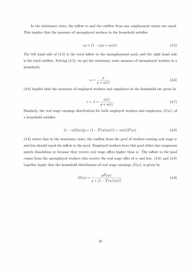
In the stationary state, the inflow to and the outflow from any employment status are equal.

This implies that the measure of unemployed workers in the household satisfies

eρ ≡ (1− u)ρ = us(v). (4.5)

The left hand side of (4.5) is the total inflow to the unemployment pool, and the right hand side

is the total outflow. Solving (4.5), we get the stationary state measure of unemployed workers in a

household,

u =ρ

ρ + s(v). (4.6)

(4.6) implies that the measures of employed workers and employees in the household are given by

e = J =s(v)

ρ + s(v). (4.7)

Similarly, the real wage earnings distribution for both employed workers and employees, G(w), of

a household satisfies

(1− u)G(w)[ρ + (1− F (w))s(v)] = us(v)F (w). (4.8)

(4.8) states that in the stationary state, the outflow from the pool of workers earning real wage w

and less should equal the inflow to the pool. Employed workers leave this pool either due exogenous

match dissolution or because they receive real wage offers higher than w. The inflow to the pool

comes from the unemployed workers who receive the real wage offer of w and less. (4.6) and (4.8)

together imply that the household distribution of real wage earnings, G(w), is given by

G(w) =ρF (w)

ρ + (1− F (w))s(v). (4.9)

16

4.2 Existence and Uniqueness of an Equilibrium

Definition: A stationary monetary equilibrium (SME) with dispersed real wages is defined as a

collection of variables c,M, v, v, u, u, w and distributions F (w), G(w), F (w), G(w) such that

(i) Given F (w), G(w), and v, the household choice variables c, M, v, F (w) solve (PH);

(ii) the real reservation wage of an unemployed worker w satisfies (4.2);

(iii) the unemployment rate, u, is given by (4.6);

(iv) the real wage earnings distribution, G(w), is given by (4.9);

(v) the expected return on each posted real wage offer, defined in (3.14), R(w) = R∗ ∀ w ∈ [w,w]

where w is the highest real wage posted by the household;

(vi) aggregate variables are equal to the relevant household variables, F (w) = F (w), G(w) =

G(w), v = v, u = u;

(vii) the goods market clears, Jy = c;

(viii) the marginal value of real money balances, ΩM , is strictly positive and finite.

The optimal choices of the household and the equilibrium conditions induce the following

equilibrium relations. Given that the buyer’s nominal money balance constraint binds, the goods

market clears, and in equilibrium, the measure of employed workers, e, equals the measure of

employees of the firms, J we have

M = Jy ≡ s(v)ρ + s(v)

y = c. (4.10)

(3.18) and the equilibrium condition that the expected gross return on all real wage offers

posted be equal imply that the equilibrium measure of vacancies, v, implicitly solves

k′(v) =s(v)v

ρ

ρ + s(v)ΩJ(w) (4.11)

where ΩJ(w) is the marginal value of a job at the lowest real wage offered.10 (4.11) equates the

marginal cost of posting a vacancy with the discounted expected marginal benefit from the job at

10 From (3.15), the marginal value of a job at a real wage w in the stationary state is given by

ΩJ(w) =(y − w)ΩM

(r + ρ + s(v)(1− F (w))).

17

the real reservation wage of the unemployed workers. After substituting for ΩJ(w) in (4.11), we

get

k′(v) =s(v)v

ρ

(ρ + s(v))(y − w)ΩM

(r + ρ + s(v)). (4.12)

The equilibrium condition for the measure of vacancies is similar to the equilibrium condition

derived by Mortensen (2000). The difference is that the measure of vacancies in this model depends

on the marginal value of real money balances, which is endogenously determined in the economy.

This is the consequence of embedding the Mortensen model in a cash-in-advance economy. Using

(4.2), (4.3), and (4.10), we can eliminate w and ΩM from (4.12) and get

vk′(v) = s(v)ρ

(ρ + s(v))(r + ρ + s(v))

u′

( s(v)yρ+s(v)

)

(1 + r)gy − φ

. (4.13)

It is clear from (4.13) that the solutions for the measure of vacancies, v, depend on the form of

the household utility function, u(c). Notice that in equilibrium the value of vacancies, v, is bounded

from above by v satisfying the following equation

u′( s(v)y

ρ+s(v)

)

(1 + r)gy = φ. (4.14)

Let c be the consumption associated with v. The lowest value the equilibrium measure of

vacancies, v, can take is zero, and the associated consumption will also be zero. Now, define the

coefficient of relative risk aversion as θ(c) ≡ −u′′(c)u′(c) c. Then, the following lemma characterizes the

possible solutions of v for different types of utility function.

Lemma 2:

(i) If the utility function is such that limc→0 u′(c)c → 0, then (4.13) has a solution at v = 0. In

addition, if limc→0u′(c)

(1+r)g (1− θ(c)) > φy , then (4.13) also has a solution at v > 0.

(ii) If the utility function is such that limc→0 u′(c)c > 0 and θ(c) ≥ 1, ∀ 0 ≤ c ≤ c, then (4.13) has

a unique solution at v > 0.

For the rest of the paper, we will assume that there exists a unique equilibrium level of

vacancies, v > 0. The equilibrium condition that the expected gross return on each posted real

wage offer is equal implies that, for a given v > 0, the distribution of real wage offers, F (w),

implicitly solves

18

y − w

(ρ + s(v)(1− F (w)))(r + ρ + s(v)(1− F (w)))=

y − w

(ρ + s(v))(r + ρ + s(v)), ∀ w ∈ F . (4.15)

(4.15) is a quadratic equation in the distribution of the real wage offers, F (w). The equilibrium

F (w) is the positive root of this quadratic equation and is given by

F (w) =r + 2(ρ + s(v))

2s(v)

1−

√r2 + 4(ρ + s(v))(r + ρ + s(v))y−w

y−w

(r + 2(ρ + s(v)))2

. (4.16)

Putting F (w) = 1 in (4.16), one can solve for the upper support of the real wage offer distri-

bution, w. w is given by

w = w +[1− ρ(r + ρ)

(ρ + s(v))(r + ρ + s(v))

](y − w). (4.17a)

The ratio of the upper support to the lower support, w/w, is given by

w/w = 1 +[1− ρ(r + ρ)

(ρ + s(v))(r + ρ + s(v))

](y

w− 1

). (4.17b)

The equations for the distribution of the real wage offers and its upper support are identical in

form to the ones derived in the Mortensen (2000). However, the crucial difference here is that in the

current model, unlike that of Mortensen (2000), the real reservation wage of unemployed workers,

w, and the measure of vacancies, v, depend on the endogenously determined marginal value of real

money balances.

For a unique and finite equilibrium v > 0, the marginal value of real money balances, ΩM , is

strictly positive and finite. Hence, we have following proposition.

Proposition 1: For a unique, strictly positive, and finite equilibrium level of vacancies, there

exists a unique SME with dispersed real wages characterized by equations 4.2, 4.3, 4.9, 4.16, and

4.17a.

In the next section, we turn to analyze the effects of inflation rate on output and welfare.

19

5. Inflation, Output, and Welfare

The effects of inflation on consumption, output, and employment are summarized in the fol-

lowing proposition.

Proposition 2: An increase in the inflation rate in the SME with dispersed real wages reduces

vacancies, consumption, and output, and increases the unemployment rate.

An increase in the inflation rate erodes the value of fiat money, which reduces the return of

firms on vacancies for a given level of consumption. In addition, higher inflation rate reduces the

expected benefit from working and increases the real reservation wage of unemployed workers for

a given consumption level, which further lowers the return on vacancies. This induces firms to

reduce the equilibrium level of vacancies posted, which leads to lower output and consumption and

a higher unemployment rate.11

The effect of inflation on employment and consumption in the SME with dispersed real wages

is similar to that in standard cash-in-advance economies (e.g. Cooley and Hansen 1989), where an

increase in the inflation rate induces households to shift from consumption goods, which require

cash, to leisure, which does not require cash.

In the SME with dispersed real wages, however, a fall in consumption and output does not

necessarily lead to a fall in social welfare. To see this, we compare the social optimal level of

vacancies with the level of vacancies in the SME with dispersed real wages. The social planner

maximizes

maxct,vt,ut+1

∞∑t=0

1(1 + r)t

[u(ct)− (1 + φ)(1− ut)− ut − k(vt)

]

subject to

ut+1 = ρ(1− ut) + (1− s(vt))ut ∀ t (5.1)

11 The result that consumption and output necessarily fall with inflation is because we do not allow match-specific investment. If we allow match-specific investment, consumption and output need not fall withinflation even though the level of vacancies decline. The reason is that a fall in the level of vacancies byreducing the turnover of employed workers encourages firms to incur higher match-specific investment,which by increasing workers’ productivity may more than offset the decline in output due to higherunemployment. Kumar (2003) develops similar mechanism in a non-monetary setup in which higherunemployment benefits can increase output.

20

ct = y(1− ut) ∀ t. (5.2)

The first constraint is the labor matches constraint, which indicates that next period’s level

of unemployment equals the sum of the measure of employed workers who become unemployed in

the current period and the measure of unemployed workers of the current period who are unable

to find job. The second constraint is the feasibility constraint on consumption goods.

In the stationary state, the optimal level of vacancies is given by (see Appendix 2)

k′(v) =ρs′(v)

(ρ + s(v))(r + ρ + s(v))

[u′

( s(v)yρ + s(v)

)y − φ

]. (5.3)

It can be easily shown that (5.3) has a unique solution. Let the elasticity of matching function

with respect to vacancy be η ≡ s′(v)vs(v) .12 The following proposition compares the social optimal

level of vacancies with the market equilibrium level of vacancies.

Proposition 3: In the SME, the optimal inflation rate, g∗, exceeds the Friedman rule and is

implicitly given by

g∗ =1

(1 + r)[η + (1−η)φ

u′(c(g∗))y

] >1

1 + r(5.4)

The optimal inflation rate exceeds the Friedman rule because here, the inflation rate affects

the real reservation wage of unemployed workers, which, in turn distorts the level of vacancies

posted by firms. The economy has two sources of inefficiency — the binding buyer’s nominal cash

balance constraint and the undirected search by workers allowing firms to hire workers at the real

reservation wage. If the real reservation wage of unemployed workers is low, firms create too many

vacancies. As the inflation rate falls, the real reservation wage of the unemployed workers declines

for a given consumption level increasing the expected return on vacancies. Consequently, as the

inflation rate approaches the Friedman rule, firms create too many vacancies and the unemployment

rate falls too low relative to the social optimum.

12 Given the assumptions about the matching function, 0 < η < 1.

21

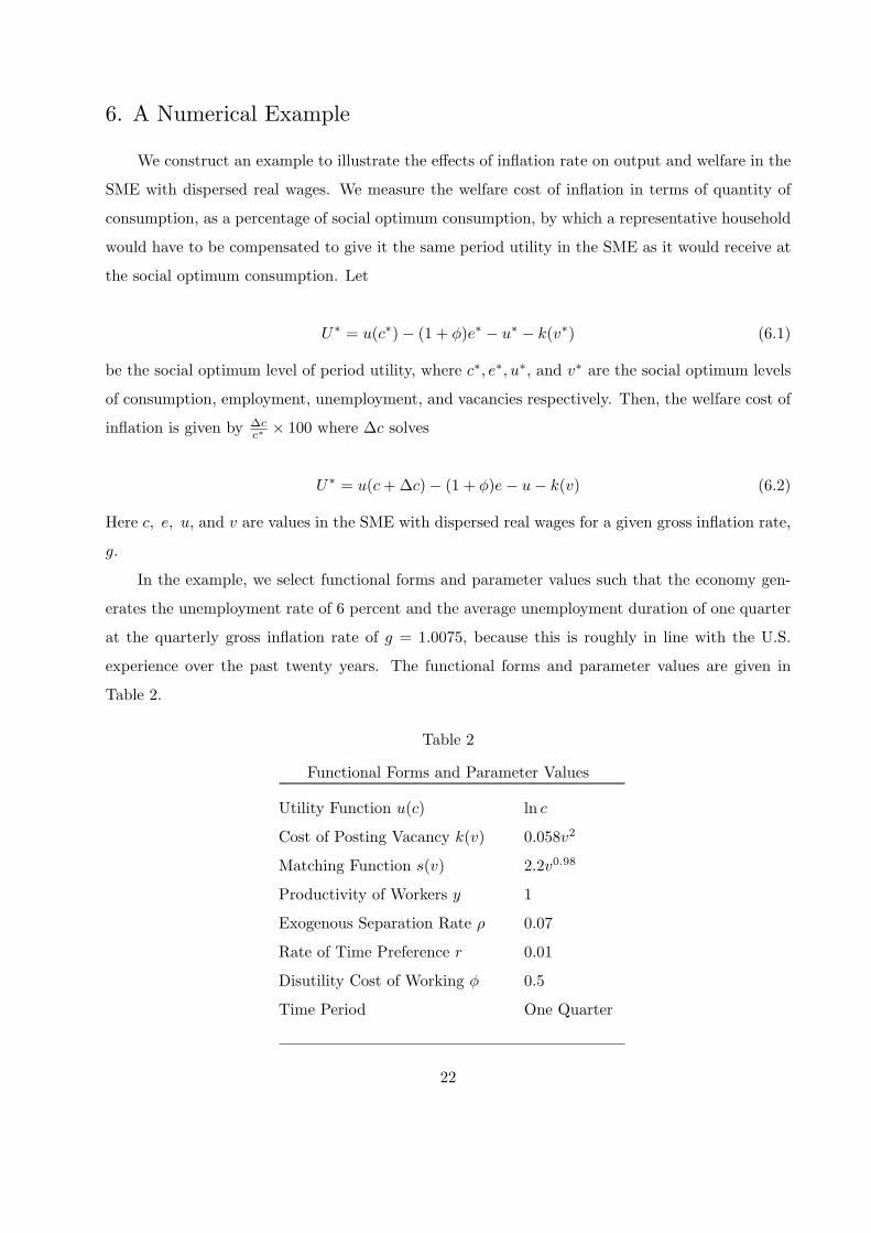
6. A Numerical Example

We construct an example to illustrate the effects of inflation rate on output and welfare in the

SME with dispersed real wages. We measure the welfare cost of inflation in terms of quantity of

consumption, as a percentage of social optimum consumption, by which a representative household

would have to be compensated to give it the same period utility in the SME as it would receive at

the social optimum consumption. Let

U∗ = u(c∗)− (1 + φ)e∗ − u∗ − k(v∗) (6.1)

be the social optimum level of period utility, where c∗, e∗, u∗, and v∗ are the social optimum levels

of consumption, employment, unemployment, and vacancies respectively. Then, the welfare cost of

inflation is given by ∆cc∗ × 100 where ∆c solves

U∗ = u(c + ∆c)− (1 + φ)e− u− k(v) (6.2)

Here c, e, u, and v are values in the SME with dispersed real wages for a given gross inflation rate,

g.

In the example, we select functional forms and parameter values such that the economy gen-

erates the unemployment rate of 6 percent and the average unemployment duration of one quarter

at the quarterly gross inflation rate of g = 1.0075, because this is roughly in line with the U.S.

experience over the past twenty years. The functional forms and parameter values are given in

Table 2.

Table 2

Functional Forms and Parameter Values

Utility Function u(c) ln c

Cost of Posting Vacancy k(v) 0.058v2

Matching Function s(v) 2.2v0.98

Productivity of Workers y 1

Exogenous Separation Rate ρ 0.07

Rate of Time Preference r 0.01

Disutility Cost of Working φ 0.5

Time Period One Quarter

22

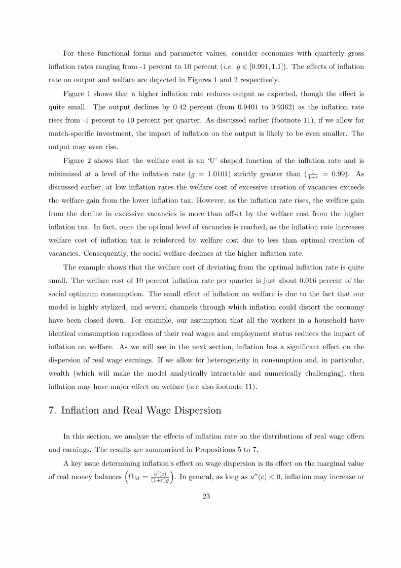
For these functional forms and parameter values, consider economies with quarterly gross

inflation rates ranging from -1 percent to 10 percent (i.e. g ∈ [0.991, 1.1]). The effects of inflation

rate on output and welfare are depicted in Figures 1 and 2 respectively.

Figure 1 shows that a higher inflation rate reduces output as expected, though the effect is

quite small. The output declines by 0.42 percent (from 0.9401 to 0.9362) as the inflation rate

rises from -1 percent to 10 percent per quarter. As discussed earlier (footnote 11), if we allow for

match-specific investment, the impact of inflation on the output is likely to be even smaller. The

output may even rise.

Figure 2 shows that the welfare cost is an ‘U’ shaped function of the inflation rate and is

minimized at a level of the inflation rate (g = 1.0101) strictly greater than ( 11+r = 0.99). As

discussed earlier, at low inflation rates the welfare cost of excessive creation of vacancies exceeds

the welfare gain from the lower inflation tax. However, as the inflation rate rises, the welfare gain

from the decline in excessive vacancies is more than offset by the welfare cost from the higher

inflation tax. In fact, once the optimal level of vacancies is reached, as the inflation rate increases

welfare cost of inflation tax is reinforced by welfare cost due to less than optimal creation of

vacancies. Consequently, the social welfare declines at the higher inflation rate.

The example shows that the welfare cost of deviating from the optimal inflation rate is quite

small. The welfare cost of 10 percent inflation rate per quarter is just about 0.016 percent of the

social optimum consumption. The small effect of inflation on welfare is due to the fact that our

model is highly stylized, and several channels through which inflation could distort the economy

have been closed down. For example, our assumption that all the workers in a household have

identical consumption regardless of their real wages and employment status reduces the impact of

inflation on welfare. As we will see in the next section, inflation has a significant effect on the

dispersion of real wage earnings. If we allow for heterogeneity in consumption and, in particular,

wealth (which will make the model analytically intractable and numerically challenging), then

inflation may have major effect on welfare (see also footnote 11).

7. Inflation and Real Wage Dispersion

In this section, we analyze the effects of inflation rate on the distributions of real wage offers

and earnings. The results are summarized in Propositions 5 to 7.

A key issue determining inflation’s effect on wage dispersion is its effect on the marginal value

of real money balances(ΩM = u′(c)

(1+r)g

). In general, as long as u′′(c) < 0, inflation may increase or

23

reduce the marginal value of real money balances. Under certain restrictions, however, an increase

in the rate of inflation unambiguously reduces the marginal value of real money balances.

Lemma 3: If in the SME ρ(r + ρ) ≤ s2(v), then an increase in the inflation rate reduces the

marginal value of real money balances, ΩM .

Lemma 3 states that if the rate of time preference and the exogenous separation rate are

small relative to the matching rate of workers, then the inflation rate reduces the marginal value of

real money balances. The empirical evidence on the matching rate of workers and the exogenous

separation rate suggests that in the real economies this condition is likely to be satisfied. For

example, in the U.S. the average duration of unemployment is approximately one quarter. If we

set the time-period to be a quarter, then this implies that s(v) = 1. The exogenous separation rate

per quarter is variously estimated to be between 0.005 to 0.11. Also in the macro literature, the

rate of time preference per quarter is commonly assumed to be 0.01. This suggests that the above

condition is satisfied for the U.S. economy. Note that this condition is also satisfied in the example

introduced in the Section 6.

If the condition in Lemma 3 is satisfied, the real reservation wage of unemployed workers

must rise as inflation increases. A reduction in the marginal value of real money balances reduces

the expected benefit from working (4.2), and thus for a given disutility cost of working the real

reservation wage w must rise in order to induce the unemployed workers to accept work.

Proposition 4: Let ρ(r + ρ) ≤ s2(v) in the SME. Then, an increase in the inflation rate reduces

the support of the distributions of real wage offers and earnings in the sense that w/w falls (the

range falls as well).

Inflation affects the support of the distributions of real wage offers and earnings through its

effect on the real reservation wage of the unemployed workers and the level of vacancies. An increase

in the inflation rate increases the real reservation wage of unemployed workers and raises the lower

support of the distributions of both real wage offers and earnings. An increase in the inflation rate

may also raise the upper support. But this effect is mitigated by two factors.

Firstly, firms posting the highest real wage do not face any competition from other firms to

retain their workers. On the other hand, firms posting lower real wages face competition from

other firms to retain their workers. Consequently, firms posting the highest real wage need not

increase their wages as much as the firms posting the lowest real wage. Secondly, vacancies decline

24

with an increase in the inflation rate reducing the matching rate of workers and weakening the

effectiveness of on-the-job search in reducing the market power of firms. If the second factor is

strong enough, then the upper support may in fact fall. These two factors imply that the support

of the distributions of real wage offers and earnings falls with an increase in the inflation rate as

long as the exogenous separation rate and the rate of time preference are small compared to the

matching rate of workers.

If the condition ρ(r + ρ) ≤ s2(v) is not satisfied, the real reservation wage of unemployed

workers may rise or fall with the inflation rate. If the real reservation wage of unemployed workers

falls, then one can show that the higher inflation rate may increase or reduce the support of the

distributions of real wage offers and earnings.

While analytically we are only able to show that higher inflation reduces the support of the

distributions of real wage offers and earnings (under plausible conditions), through numerical com-

putations it can be shown that a higher inflation rate reduces the dispersions of real wages.13

Figure 3 depicts the lower and upper supports of the distributions of real wage offers and earnings

generated using the numerical example introduced in the Section 6. The figure shows that higher

inflation rate increases the lower support (from .5001 to .5693), while it has little impact on the

upper support reducing the range of real wage offers and earnings.

Figure 4 depicts the coefficients of variations of real wage offers and earnings. Figure 5 shows

the ratios of 90th to 10th percentile, 90th to 50th percentile, and 50th to 10th percentile of the real

wage offers distribution. Figure 6 plots the same ratios of the distribution of real wage earnings.

All these figures show that a higher inflation rate reduces the dispersion of real wage offers and

earnings. Quantitative experiments indicate that higher inflation reduces the dispersion in real

wage offers and earnings for a wide range of parameter values and functional forms. The result of

our model is consistent with empirical observation that inflation is associated with reduced wage

dispersion.

Given that inflation affects the distributions of real wage offers and earnings, it is interesting

to ask the question whether the household would prefer the distributions of real wage offers and

earnings associated with higher inflation or lower inflation. The following two propositions address

this issue.

13 It is well-known that the basic Mortensen (2000) model generates increasing wage offers and earningsdensities, which are not supported empirically. However, this is the consequence of the assumption thatthe firms are of identical productivity. By introducing heterogeneous firms, one can match a variety ofwage offers and earnings densities (e.g. Bontemps et. al. (2000)).

25

Proposition 5: Let ρ(r + ρ) ≤ s2(v) and r be small (r2 ≈ 0). Then, an increase in the inflation

rate may or may not lead to a stochastic improvement in the distribution of real wage offers, F (w).

An increase in the inflation rate has two conflicting effects on the market power of firms. Firstly,

an increase in the inflation rate, if it increases the real reservation wage of unemployed workers,

reduces the market power of firms and leads to stochastic improvement in the distribution of the

real wage offers. Secondly, an increase in the inflation rate reduces the level of vacancies increasing

the market power of firms which may prevent any stochastic improvement in the distribution of

the real wage offers. In this case, the effect of the inflation rate on the average real wage offer is

ambiguous.

If the real reservation wage of unemployed workers falls, it can be shown that the proportion of

low real wage offers rises. This happens because a fall in the real reservation wage of the unemployed

workers increases the market power of firms unambiguously, and firms post a greater proportion of

low wage vacancies. In this case, the average real wage offer necessarily falls.

Proposition 6: If there is stochastic improvement in the distribution of real wage offers, F (w),

an increase in the inflation rate may or may not lead to stochastic improvement in the distribution

of real wage earnings, G(w). If there is no stochastic improvement in F (w), then the proportion of

employed workers with low real wage earnings increases with the rise in the inflation rate.

An increase in the inflation rate reduces the matching rate of workers and lowers the rate

at which employed workers move from low wage jobs to high wage jobs. Ceteris paribus, this

shifts the mass of employed workers from high wage jobs to low wage jobs. If there is a stochastic

improvement in the distribution of the real wage offers, F (w), then it may prevent the shift of mass

of employed workers from high wage jobs to low wage jobs caused by a fall in the matching rate

of the workers. However, if there is no stochastic improvement in the distribution of the real wage

offers, then the proportion of employed workers with low wage jobs rises unambiguously. In this

case, the average real wage earnings falls as the inflation rate goes up.

Figure 7 depicts the effect of inflation on the average real wage offer and earnings. The figure

shows that inflation increases both the average real wage offer and the average real wage earnings.

Quantitative experiments show that while the average real wage offer increases with inflation for

a wide range of parameter values and functional forms, this is not the case with the average real

wage earnings.

26

8. Robustness

In this section, we discuss several extensions of our model. The Burdett and Mortensen (1998)

model (on which Mortensen 2000 is based) puts severe restrictions on the wage setting behavior

of firms. Firstly, it assumes that firms cannot change their posted wages. Secondly, they do

not respond when their employees receive higher wage offers from other firms even though losing

employees is costly. Thirdly, each firm is required to offer the same posted wage to all the workers

it comes in contact with regardless of the reservation wages of the workers and thereby forgo a

part of its rent. In this section, we discuss whether the result that inflation reduces real wage

dispersion survives when firms are allowed more flexibility in setting their wages. We also discuss

how endogeneity of search intensity may modify our results.

8.1 Alternative Wage Posting Mechanisms

Coles (2001) relaxes the assumption that firms pre-commit to particular wage offers and allows

firms to change their wages anytime they like. In other aspects, Coles is identical to the basic

Burdett-Mortensen. Allowing firms to change their posted wages complicates the model a great

deal. The optimal quit decisions of the workers depend on the expected future wages at their current

employers, and those expectations must be consistent with the firms’ wage setting strategies. Coles

derives conditions under which firms do not wish to change the posted wages in the future period

(i.e. pre-committed constant wage trajectory as in Burdett-Mortensen remains an equilibrium).17

Given the workers’ beliefs that firms will not change the posted wages ever in future, the

marginal values of unemployed workers and employed workers at different wages, and thus the real

reservation wage of unemployed workers, satisfy the same functional equations as in the Burdett-

Mortensen (see Coles 2001, equation 9, page 168). Thus, with Coles’s set-up in our monetary

model, the real reservation wage of unemployed workers will still be given by (4.2) (φ = wΩM ).

The ratio of the upper and lower supports of the distributions of real wage offers and earnings

is given by (see Coles 2001, Lemma 4, page 169-170)

w/w = 1 +(

y

w− 1

)[s(v)(2ρ + s(v))

(ρ + s(v))(r + ρ + s(v))

](8.1)

17 As the rate of time-preference r → 0, the Coles equilibrium converges to Burdett-Mortensen equilibrium.

27

where s(v) indicates the fact that the job arrival rate is fixed in the model. One can immediately

see that d(w/w)dw < 0. Therefore, if the marginal value of real money balances falls, the support will

decline.

One can endogenize the job arrival rate (level of vacancies) by equating the marginal value of

vacancy with the real reservation wage of the unemployed workers to zero. Simple differentiation

of (8.1) shows that d(w/w)dw < 0 necessarily if dv

dw < 0, which will be the case because an increase in

w reduces the expected return on vacancies. Thus our findings with regard to the effect of inflation

on wage dispersions are robust to relaxing the assumption that firms pre-commit to the posted

wage offers.

Postel-Vinay and Robin (2002) modify the Burdett-Mortensen model by allowing firms to

counter the offers received by their employees from competing firms and to vary their wage offers

according to the characteristics of the particular workers with which they are matched (state-

dependent offers — lower wage to low reservation wage workers and higher wage to high reservation

wage workers).

For simplicity, consider their model with identical workers and identical firms. In this case,

the equilibrium wage distribution will be degenerate at a mixture of two mass points — one at the

real reservation wage of the unemployed workers , w, and one at the productivity of the workers, y,

because allowing the firms to counter alternative real wage offers made to their employees triggers

a Bertrand competition between the firms. Then in the monetary set-up, the real reservation wage

of unemployed workers satisfies (see Appendix 3)

[w +

s(v)r + ρ

y

]ΩM =

s(v)r(r + ρ)

− r + ρ

r+ (1 + φ)

[1 +

s(v)r + ρ

]. (8.2)

Since the right hand of (8.2) is constant, if the marginal value of real money balances, ΩM ,

falls, the real reservation wage of unemployed workers, w, must rise, which will reduce the support

of the distributions of real wage offers and earnings.

8.2 Endogenous Search Intensity

So far, we have assumed that search-intensity of workers is equal and exogenously given.

Search-intensity of workers can be endogeneized by allowing the household to optimally choose

search-intensities for workers. In such a case, the optimal choice of search-intensities will depend

on the expected gain from search. Since, the expected gain from search varies with the employment

status as well as real wage a worker earns, corresponding to the distribution of real wage earnings,

28

there will be a distribution of search intensities. Since workers earning the highest real wages have

no incentive to search, their search-intensity will be zero, while the search intensity of the workers

earning the real reservation wage will be the highest.

Since, the expected gain from search is identical for both unemployed workers as well as

employed workers earning the real reservation wage, they will have identical search intensities.

Thus, the real reservation wage of unemployed workers will continue to be given by (4.2). However,

with endogenous search intensity, the matching function is modified. Let χ(w) be the optimally

chosen search intensity at the real wage w. The total search intensity, χ, then is given by

χ = χ(w)ut + et

∫ w

w

χ(x)dG(x). (8.3)

The matching function can be written as

M(v, χ). (8.4)

Let θ ≡ vχ denote the labor market tightness, then with constant returns to scale matching function,

the matching rate of an employed worker at real wage w is given by

χ(w)m(θ), ∀ w, (8.5)

where m(θ) = M(v,χ)χ . The matching rate of an unemployed worker is given by

χ(w)m(θ), (8.6)

and the matching rate of vacancy is given by

m

(1θ

)(8.7)

.

Turning to the effects of inflation, higher inflation rate reduces the expected gain from working

and searching for a given level of consumption and labor market tightness. This leads to decline in

search intensities reducing the matching rate of workers. This reduces the workers’ turnover, which

encourages firms to post more vacancies. The decline in search intensities also increases the labor

market tightness for a given level of vacancy. This second effect by reducing the matching rate of

vacancies lowers the expected return on vacancies inducing firms to reduce the level of vacancies

29

posted. Thus, with endogenous search intensity, the effect of inflation on vacancies and thereby on

dispersion of real wages is ambiguous.

9. Minimum Wage

In this section, we consider the effect of changes in the real minimum wage on equilibrium

variables. Let us assume that the mandated real minimum wage, wmin, is binding i.e. it is higher

than the real reservation wage of the unemployed workers, w, for a given set of parameters (also

wmin < y). In this case, the real minimum wage will be the lower support of the distributions of

real wage offers and earnings.

The equilibrium level of vacancies is given by

k′(v) =s(v)v

ρ

(ρ + s(v))(y − wmin)ΩM

(r + ρ + s(v)). (9.1)

The following lemma characterizes the solution of (9.1).

Lemma 4: Let u(c) = c1−θ

1−θ and θ ≥ 1, then (9.1) has a unique and finite solution v > 0.

For a unique and finite equilibrium level of vacancies, there will be a unique equilibrium and

the associated distribution of real wage offers, F (w), and the upper support w are continued to be

given by (4.16) and (4.17) respectively with the real reservation wage w being replaced by the real

minimum wage wmin.

The following proposition summarizes the effect of inflation and the real minimum wage on

the equilibrium variables.

Proposition 7: Let the real minimum wage be binding:

(i) For a given real minimum wage, an increase in the inflation rate reduces the level of vacancies

and the support of the distributions of real wage offers and earnings, w/w (range falls too).

(ii) For a given inflation rate, an increase in the real minimum wage has the same effect.

For a given real minimum wage, higher inflation reduces the return on vacancies and firms cut

down the number of vacancies posted. The decline in the number of vacancies posted reduces the

effectiveness of on-the-job search in weakening the market power of firms and the highest real wage

posted falls lowering the support. In this case, the support falls solely due to the fall in the upper

support of the wage distributions. It is also easy to show that with the binding real minimum

30

wage the effects of inflation on vacancies and w/w are smaller than they would be when the real

minimum wage is non-binding.

For a given inflation rate, an increase in the real minimum wage by lowering the return of firms

on vacancies reduces the level of vacancies posted. This coupled with the increased lower support

leads to compression in the support of the distributions of real wage offers and earnings. Mortensen

(2000) derives this result in a non-monetary partial equilibrium set-up. We show that this result

holds in a general equilibrium monetary set-up.

Quantitative experiments (not depicted) show that higher real minimum wage reduces other

measures of dispersion. These results are consistent with empirical findings that the decline in the

real minimum wage increases wage dispersion.

10. Conclusion

This paper has analyzed the effects of inflation on the dispersion of real wage earnings and

welfare in a cash-in-advance economy with search friction in the labor market. The paper shows that

in equilibrium an increase in the inflation rate reduces real wage dispersion, a finding consistent

with those of several empirical papers. This result is robust to several variations in the wage

posting process. An increase in the inflation rate also reduces the level of vacancies and output

and increases the unemployment rate. In addition, the Friedman rule is not optimal. Because of

undirected search by workers, the optimal inflation rate exceeds the rate of discount. The paper

also shows that the decline in the real minimum wages increases the dispersion of real wages by

affecting the entire distribution, which is consistent with empirical findings.

The paper proposes a mechanism through which higher inflation can reduce wage dispersion.

We would like to examine the quantitative significance of this mechanism. In future work, we would

also like to examine the effects of inflation on the composition of vacancies (more or less skilled

jobs) and inter-skill wage dispersion.

31

Appendix 1: Proofs

Lemma 1:

(i) The Optimal Job Acceptance Strategies of Employed Workers

The household prescribes the job-acceptance strategies to workers, which maximizes its ex-

pected return. Suppose that the household instructs employed workers not to accept any new real

wage offer and continue to work at their current real wages. The expected return at time t to the

household on the measure of employed workers earning real wage w and less, etGt(w), is given by

Ret′(w) ≡ etGt(w)

[ωMt

∫ w

w

xdGt(x)− (1 + φ) + Et

∞∑

i=t

li+1

(1 + r)i+1−t

](A1.1)

where

li+1 = −1,with probability ρ

= ωMi+1pi+1

w∫

w

xdGi(x)− (1 + φ), with probability (1− ρ)∀ i. (A1.2)

The future return li+1 reflects the fact that employed workers may become unemployed with

probability ρ.

Suppose now that the household instructs employed workers to accept any offer which gives

them real wages higher than what they currently earn. In this case, the return to the household

on the measure of employed workers earning real wages w and less is

Ret′′(w) ≡ etGt(w)

[ωMt

∫ w

w

xdGt(x)− (1 + φ) + Et

∞∑

i=t

li+1

(1 + r)i+1−t

](A1.3)

where

li+1 = −1,with probability ρ

=

ωMi+1pi+1

∫ w

w

[[(1− Fi(x))

∫ w

x

zdFi(z)] + Fi(x)x]dGi(x)− (1 + φ),

with probability s(vi)

ωMi+1pi+1

∫ w

w

xdGi(x)− (1 + φ), with probability(1− ρ− s(vi))

∀i. (A1.4)

32

Comparing A1.2 to A1.4, we can immediately see that Ret′′(w) > Ret

′(w). By similar reasoning

one can show that it is not optimal for the household to instruct employed workers to accept real

wage offers lower than what they currently earn. Therefore, the household instructs employed

workers to accept any real wage offer higher than what they currently earn.

ii) The optimal real reservation wage of unemployed workers

Let

St(w) = Set of workers receiving real wage offer of less than w

S′t(w) = The complement set of St(w)

wi = Wage offer received by worker i

Ret(w′ ≤ w ≤ w′′) = Expected return on the measure of employed workers receiving wage

greater than or equal to w′ but less than or equal to w′′.

Suppose that the household prescribes unemployed workers to accept any real wage offer x ≥ w.

Then the expected return to the household on the measure of unemployed workers at time t, ut, is

Rut(w) =− ut +1

1 + r

[

− ut(1− s(vt))−∫

i∈St(w)

di

+∫

i∈S′t(w)

(xiωMt+1pt+1 − (1 + φ)

)di

+ Nt+1(w)]

∀ t (A1.5)

where Nt+1(w) is the discounted future stream of utilities defined as

Nt+1(w) =

Rutht(w), for the unemployed workers at time t

who stay unemployed at time t + 1 where

ht = ut[1− st(vt)(1− Ft(w))] and

Ret+1(w ≤ x ≤ w), for the unemployed workers who accept the job offers

∀ t. (A1.6a)

where

Ret+1(w ≤ w ≤ w) ≡

utst(vt)(1− Ft(w))

[ωMt+2

∫ w

w

xdGt+2(x)− (1 + φ) + Et

∞∑

i=t+2

li+1

(1 + r)i+1−t

](A1.6b)

33

where

li+1 = −1,with probability ρ

=

ωMi+1pi+1

∫ w

w

[[(1− Fi(x))

∫ w

x

zdFi(z)] + Fi(x)x]dGi(x)− (1 + φ),

with probability s(vi)

ωMi+1pi+1

∫ w

w

xdGi(x)− (1 + φ), with probability(1− ρ− si(vi))

∀i. (A1.6c)

Note that the measure of unemployed workers receiving real wage offers less than w is

utst(vt)Ft(w), and the measure of unemployed workers receiving real wage offers of w and higher

is utst(vt)(1− Ft(w)).

Now suppose that w < w∗ where w∗ satisfies ωMt+1pt+1w∗ = φ. In this case, one can

immediately show that Rut(w∗) > Rut(w) since

∫

i∈S′t(w∗)

(xiωMt+1pt+1 − (1 + φ)

)di−

∫

i∈St(w∗)di >

∫

i∈S′t(w)

(xiωMt+1pt+1 − (1 + φ)

)di−

∫

i ∈St(w)

di ∀ t. (A1.7)

By similar logic we can show that Rut(w∗) > Rut(w) if w > w∗. Therefore, it is optimal for

the household to instruct unemployed workers to accept any real wage offer w ≥ w∗.

Lemma 2:

The equilibrium value of vacancies, v, is given by

vk′(v) =ρ

r + ρ + s(v)

[u′(c)c

(1 + r)g− φ

yc

]≡ T (v). (A1.8)

From the above, it is clear that when u′(c)c = 0 for c = 0, then (A1.8) has solution v = 0.

But, when u′(c)c > 0 for c = 0, then (A1.8) does not have solution at v = 0 and T (v) > vk′(v).

From, (A1.8), it is also clear that the maximum value, which c or v can take is given by

u′(c)(1 + r)g

=φ

y. (A1.9)

Denote the solution of (A1.9) by c. It is also clear that at c, vk′(v) > T (v).

34

Differentiating T (v) w.r.t. v, we get

T ′(v) =ρ

(r + ρ + s(v))2[ (r + ρ + s(v))yρ

(ρ + s(v))2[u′′(c)c + u′(c)

(1 + r)g− φ

y

]

−[ u′(c)c(1 + r)g

− φ

yc]]

s′(v)

.

(A1.10)

The coefficient of relative risk aversion is given by −u′′(c)cu′(c) ≡ θ(c). Then, (A1.10) can be

written as

T ′(v) =ρ

(r + ρ + s(v))2[ (r + ρ + s(v))yρ

(ρ + s(v))2[u′(c)(1− θ(c))

(1 + r)g− φ

y

]

−[ u′(c)c(1 + r)g

− φ

yc]]

s′(v). (A1.11)

From (A1.11), it is clear that in the case θ(c) ≥ 1, ∀ 0 ≤ c ≤ c, T ′(v) < 0. Thus, in the case

u′(c)c > 0 when c = 0, there exists a unique solution.

(A1.11) also shows that when limc→0u′(c)

(1+r)g (1 − θ(c)) > φy , then T ′(v) → ∞ when c → 0

since limv→0 s′(v) → ∞. Thus, in the case limc→0 u′(c)c → 0, there exists at least one non-trivial

solution.

Proposition 2:

The equilibrium level of vacancies is given by

vk′(v) =ρ

r + ρ + s(v)

[u′(c)c

(1 + r)g− φ

yc

]≡ T (v). (A1.12)

We can immediately see that

dT (v)dg

< 0. (A1.13)

From (A1.13), it follows that when equilibrium is unique, an increase in the inflation rate

reduces the equilibrium level of vacancies and thus employment, consumption, and output.

Proposition 3:

The market equilibrium level of vacancies is given by

vk′(v) = s(v)ρ

(ρ + s(v))(r + ρ + s(v))

[u′(c)

(1 + r)gy − φ

]. (A1.14)

35

The social optimum level of vacancies is given by

k′(v) =ρs′(v)

(ρ + s(v))(r + ρ + s(v)[u′(c)y − φ]. (A1.15)

Now, define the elasticity of matching function w.r.t. vacancy η ≡ s′(v)vs(v) . (A1.14) and (A1.15)

imply that the market and the social levels of vacancies will be equal at the inflation rate g satisfying

η[u′(c)y − φ] =[

u′(c)y(1 + r)g

− φ

]. (A1.16)

Simplifying, we get the optimal rate of g∗

g∗ =1

(1 + r)[η + (1−η)φ

u′(c)y

] . (A1.17)

From (A1.17), it is clear that the Friedman rule is optimal only when η = 1. But, given the

restrictions on the matching function 0 < η < 1. Also, in equilibrium, u′(c)y > φ, which implies

that

g∗ >1

1 + r. (A1.18)

Lemma 3:

The equilibrium level of vacancies is given by

vk′(v) =ρ

r + ρ + s(v)

[u′(c)c

(1 + r)g− φ

yc

]≡ T (v, g) (A1.19)

where c = s(v)yρ+s(v) . Now let

Z(v) ≡ s(v)(ρ + s(v))(r + ρ + s(v))

. (A1.20)

Factoring out c from the RHS of (A1.20) and using the definition of Z(v), we have

T (v, g) ≡ Z(v)ρy

[ΩM (g)− φ

y

]. (A1.21)

.

Differentiating Z(v) w.r.t. v we get

36

Z ′(v) =s′(v)

(ρ + s(v))2(r + ρ + s(v))2[ρ(r + ρ)− s2(v)]. (A1.22)

From (A1.22), it is clear that Z ′(v) ≤ 0 if ρ(r + ρ) ≤ s2(v) and Z ′(v) > 0 otherwise.

Let the initial equilibrium satisfy v∗k(v∗) = T (v∗, g∗). Now suppose that the gross inflation

rises to g′ (g′ > g∗). From the Proposition 2, we know that at new equilibrium v′ < v∗ and

T (v′, g′) < T (v∗, g∗).

Case I: Z ′(v) ≤ 0

In this case, Z(v′) ≥ Z(v∗). Thus, in order to have T (v′, g′) < T (v∗, g∗), from (A1.22) it must

be the case that ΩM (g′) < ΩM (g∗). In this case, the marginal value of real money balances falls

unambiguously with an increase in the inflation rate, g.

Case II: Z ′(v) > 0

In this case, Z(v′) < Z(v∗) and ΩM (g′) can be higher or lower than ΩM (g∗). Therefore, in

this case the effect of inflation rate on the marginal value of real money balances is ambiguous.

Proposition 4:

w/w = 1 +[1− ρ(r + ρ)

(ρ + s(v))(r + ρ + s(v))

](y

w− 1

). (A1.23)

Differentiating (A1.23) w.r.t. g we get

d (w/w)dg

=−[1− ρ(r + ρ)

(ρ + s(v))(r + ρ + s(v))

](y

w2

)dw

dg

+ρ(r + ρ)

(ρ + s(v))2(r + ρ + s(v))2

(y

w− 1

)(r + 2ρ + 2s(v))s′(v)

dv

dg

. (A1.24)

Given that dvdg < 0, if dw

dg > 0, then d(w/w)dg < 0. If dw

dg < 0, then d(w/w)dg is of ambiguous sign.

Proposition 5:

The real wage offer distribution F (w) is given by

F (w) =r + 2(ρ + s(v))

2s(v)

1−

√r2 + 4(ρ + s(v))(r + ρ + s(v))y−w

y−w

(r + 2(ρ + s(v)))2

. (A1.25)

Let L ≡ (r + 2(ρ + s(v)))2. Then,

37

dL

dg= 4(r + 2ρ + 2s(v))s′(v)

dv

dg. (A1.26)

Let H ≡ r2 + 4(r + ρ + s(v))(ρ + s(v))y−wy−w . Then,

dH

dg=

4(y − w)(y − w)2

[(y − w)(r + 2ρ + 2s(v))s′(v)

dv

dg+ (ρ + s(v))(r + ρ + s(v))

dw

dg

]. (A1.27)

Differentiating (A1.27) w.r.t. g, we get

dF (w)dg

=−[1−

√H

L

](r + 2ρ)s′(v)

2s(v)2dv

dg

− 2(

H

L

)−1/2r + 2(ρ + s(v))

s(v)L2

2L(y − w)(y − w)2

[(y − w)(r + 2ρ + 2s(v))s′(v)

dv

dg

+ (r + ρ + s(v))(ρ + s(v))dw

dg

]+ 2

(H

L

)−1/2

r + 2(ρ + s(v))s(v)L2

[r2 + 4(ρ + s(v))(r + ρ + s(v))

y − w

y − w

](r + 2ρ + 2s(v))s′(v)

dv

dg

(A1.28)

Rearranging and simplifying (A1.28), we get

dF (w)dg

=−[1−

√H

L

](r + 2ρ)s′(v)

2s(v)2dv

dg

− 2(y − w)(ρ + s(v))(r + ρ + s(v))r + 2(ρ + s(v))Ls(v)(y − w)2

(H

L

)−1/2dw

dg− 2

(H

L

)−1/2

(r + 2(ρ + s(v)))2

s(v)L2

[L(y − w)y − w

− (r2 + 4(ρ + s(v))(r + ρ + s(v))

y − w

y − w

)]s′(v)

dv

dg(A1.29)

Now L ≡ (r + 2(ρ + s(v)))2 ≡ r2 + 4(ρ + s(v))2 + 4r(ρ + s(v)). This implies that

L(y − w)y − w

− (r2 + 4(ρ + s(v))(r + ρ + s(v))

y − w

y − w

)= r2

(y − w

y − w− 1

). (A1.30)

Putting (A1.30) into (A1.29), we get

dF (w)dg

=−[1−

√H

L

](r + 2ρ)s′(v)

2s(v)2dv

dg

− 2(y − w)(ρ + s(v))(r + ρ + s(v))r + 2(ρ + s(v))Ls(v)(y − w)2

(H

L

)−1/2dw

dg

− 2(

H

L

)−1/2 (r + 2(ρ + s(v)))2

s(v)L2r2

(y − w

y − w− 1

)s′(v)

dv

dg

. (A1.31)

38

If we set r2 = 0, the proposition follows.

Proposition 6

The real wage earnings distribution G(w) is given by

G(w) =ρF (w)

ρ + s(v)(1− F (w)). (A1.32)

Differentiating (A1.32) w.r.t. g we get

dG(w)dg

=ρ

(ρ + s(v)(1− F (w)))2[(ρ + s(v))

dF (w)dg

− F (w)(1− F (w))s′(v)dv

dg

]. (A1.33)

The proposition follows from (A1.33).

Lemma 4

The equilibrium level of vacancies solves

k′(v)v =ρ(y − wmin)

(1 + r)gyθ(r + ρ + s(v))

(ρ + s(v)

s(v)

)θ−1

≡ T (v) (A1.34)

Since, limv→0 T (v) > 0, there is no solution at v = 0. Simple differentiation of T (v) w.r.t v

and rearrangement shows that T ′(v) < 0. Therefore, given the properties of vk′(v) there exists a

unique, strictly positive, and finite solution to (A1.34).

Proposition 7

Simple differentiation of T (v) defined in (A1.8) shows that dT (v)dg & dT (v)

dwmin< 0. Thus, the level

of vacancies falls with the higher inflation rate and the minimum real wage.w

wminis given by

(w

wmin

)= 1 +

[1− ρ(r + ρ)

(ρ + s(v))(r + ρ + s(v))

](y

wmin− 1

). (A1.35)

Simple differentiation of (A1.35) w.r.t g and wmin shows that the support declines with the

higher inflation rate and the minimum real wage.

39

Appendix 2: The Social Planner Problem

The social planner maximizes

maxct,vt,ut+1

∞∑t=0

1(1 + r)t

[u(ct)− (1 + φ)(1− ut)− ut − k(vt)

]

subject to

ut+1 = ρ(1− ut) + (1− s(vt))ut ∀ t, (A2.1)

ct = y(1− ut). (A2.2)

Let λut and λct be the Langrangian multipliers associated with (A2.1) and (A2.2) respectively.

Then, the first order conditions for the social optimum are given by

ct : u′(ct) = λct, (A2.3)

vt : k′(vt) = −λuts′(vt)ut, (A2.4)

ut+1 : λut =1

1 + r

[φ− yλct+1 + [1− ρ− s(vt+1)]λut+1

]. (A2.5)

Combining (A2.3), (A2.4), and (A2.5), we get

k′(vt)s′(vt)ut

=1

1 + r

[u′(ct+1)y − φ +

k(1− ρ− s(vt+1))s′(vt+1)ut+1

]. (A2.6)

In the stationary state, (A2.6) reduces to

k′(v) =ρs′(v)

(ρ + s(v))(r + ρ + s(v))

[u′

(s(v)y

ρ + s(v)

)y − φ

]. (A2.7)

It can be easily shown that (A2.7) has a unique solution.

40

Appendix 3: The Real Reservation Wage in thePostel-Vinay and Robin Model

The marginal value of unemployed workers satisfies

Ωu =1

1 + r

[−1 + s(v)Ωe(w) + (1− s(v))Ωu

]. (A3.1)

The marginal value reflects the fact that unemployed workers receive only the real reservation wage

in the case of a match (unlike in Burdett-Mortensen). Since by definition, Ωu = Ωe(w), (A3.1)

simplifies to

Ωu = −1r. (A3.2)

Similarly, the marginal value of an employed worker at the real reservation wage w is given by

Ωe(w) =1

1 + r

[wΩM − (1 + φ) + ρΩu + s(v)Ωe(y) + (1− ρ− s(v))Ωe(w)

](A3.3)

which reflects the fact that once the employed worker receives alternative wage offer, his real wage

jumps to the worker’s productivity y.

The marginal value of an employed worker at the labor productivity y is given by

Ωe(y) =1

1 + r

[yΩM − (1 + φ) + ρΩu + (1− ρ)Ωe(y)

]. (A3.4)

Combining (A3.2)-(A3.4), we get the expression for the real reservation wage of unemployed

workers, w,

[w +

s(v)r + ρ

y

]ΩM =

s(v)r(r + ρ)

− r + ρ

r+ (1 + φ)

[1 +

s(v)r + ρ

]. (A3.5)

41

References:

Akerlof, G., W. T. Dickens, and G. L. Perry (1996), “The Macroeconomics of Low Inflation”,

Brookings Paper on Economic Activity, 1-59.

Allen, Steven (1987), “Relative Wage Variability in the United States: 1860-1983”, The Review of

Economics and Statistics, 617-626, November.

Benabou, R. (1988), “Search, Price Setting and Inflation”, Review of Economic Studies, 55, 353-376.

Benabou, R. (1992), “Inflation and Efficiency in Search Markets”, Review of Economic Studies, 59,

299-329.

Bontemps, C., J.-M. Robin, and G.J. van den Berg. (2000), “Equilibrium Search with Continuous

Productivity Dispersion: Theory and Non-parametric Estimation”, International Economic

Review, 43(2), 305-58.

Burdett, K and D. T. Mortensen (1998), “Wage Differentials, Employer Size, and Unemployment”,

International Economic Review, 39 (2), 257-273.

Chatterjee, S. and D. Corbae (1992), “Endogenous Market Participation and the General Equilib-

rium Value of Money”, Journal of Political Economy, 100, 615-646.

Coles, M.G. (2001), “Equilibrium Wage Dispersion, Firm Size and Growth”, Review of Economic

Dynamics, 4, 159-187.

Cooley, T. and G.D. Hansen (1989), “The Cost of Anticipated Inflation”, American Economic

Review, 79, 733-748.

Danziger, Leif (1999), “A Dynamic Economy with Costly Price Adjustments”, American Economic

Review, 89, 879-901.

Diamond, P. (1993), “Search, Sticky Prices, and Inflation”, Review of Economic Studies, 60, 53-68.

DiNardo, J., N.M. Fortin, and T. Lemieux (1996), “Labor Market Institutions and the Distribution

of Wages 1973-92: A Semiparametric Aproach, Econometrica, 64, 1001-1044.

Drazen, A. and D. Hammermesh (1987), “Inflation, Indexation, and Wage Dispersion”, Economic

Letters, 25, 225-231.

Erikson, C.L. and A. Ichino (1995), “Wage Differentials in Italy: Market Forces and Institutions”,

in R.B. Freeman and L. Katz (eds.) Differences and Changes in Wage Structures, University

of Chicago Press, IL, 265-305.

42

Erosa, A. and G. Ventura (2000), “On Inflation as a Regressive Consumption Tax”, Mimeo, Uni-

versity of Western Ontario.

Fuerst, T.S. (1992), “Liquidity, Loanable Funds, and Real Activity”, Journal of Monetary Eco-

nomics, 29, 3-24.

Hammermesh, D.(1986), “Inflation and Labor Market Adjustment”, Economica, 53, 63-73.

Head, A. and S. Shi. (2000), “A Fundamental Theory of Exchange Rates and Direct Currency

Trade”, Queen’s University Discussion Paper No. 993.

Head, A. and A. Kumar (2002), “Price Dispersion, Inflation, and Welfare”, Mimeo, Queen’s Uni-

versity, July.

Imrohroglu, A. (1992), “The Welfare Cost of Inflation with Imperfect Insurance”, Journal of Eco-

nomic Dynamics and Control, 16, 79-91.

Katz, L.F. and D. H.Autor (1999), “Changes in the Wage Structure and Earnings Inequality”,

Handbook of Labor Economics, Vol. 3A, North-Holland, 1463-1558.

Kumar, A. (2002), “Unemployment Insurance, Productivity, and Wage Dispersion”, Mimeo, Queen-

’s University, August.

Lee, D.S. (1999), “Wage Inequality in the United States During the 1980’s, Rising Dispersion or

Falling Minimum Wages”, Quarterly Journal of Economics, 114, 977-1023.

Lipsey, R. and B. Swedenborg (1999), “Wage Dispersion and Country Price Levels”, in A. Heston

and R. Lipsey (eds.), International and Inter-area Comparisons of Income, Output, and Prices:

Studies in Income and Wealth, Vol. 61, 453-477.

Lucas, R.E. (1982), “Interest Rates and Currency Prices in a Two-Country Model”, Journal of

Monetary Economics, 10, 335-59.

Lucas, R.E. (1990), “Liquidity and Interest Rates”, Journal of Economic Theory, 50, 237-264.

Merz, M. (1995), “Search in the Labor Market and the Real Business Cycle”, Journal of Monetary

Economics, 36, 269-300.

Mortensen, D.T. (2000), “Equilibrium Unemployment with Wage Posting: Burdett-Mortensen

Meet Pissarides”, Bunzel. et.al.(ed.) – Panel Data and Structural Labor Market Models,

North Holland, 281-292.

43

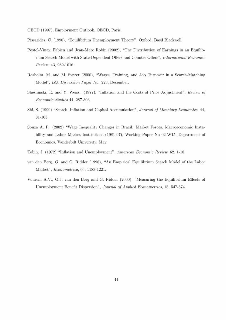
OECD (1997), Employment Outlook, OECD, Paris.

Pissarides, C. (1990), “Equilibrium Unemployment Theory”, Oxford, Basil Blackwell.

Postel-Vinay, Fabien and Jean-Marc Robin (2002), “The Distribution of Earnings in an Equilib-

rium Search Model with State-Dependent Offers and Counter Offers”, International Economic

Review, 43, 989-1016.

Rosholm, M. and M. Svarer (2000), “Wages, Training, and Job Turnover in a Search-Matching

Model”, IZA Discussion Paper No. 223, December.

Sheshinski, E. and Y. Weiss. (1977), “Inflation and the Costs of Price Adjustment”, Review of

Economic Studies 44, 287-303.

Shi, S. (1999) “Search, Inflation and Capital Accumulation”, Journal of Monetary Economics, 44,

81-103.

Souza A. P., (2002) “Wage Inequality Changes in Brazil: Market Forces, Macroeconomic Insta-

bility and Labor Market Institutions (1981-97), Working Paper No 02-W15, Department of

Economics, Vanderbilt University, May.

Tobin, J. (1972) “Inflation and Unemployment”, American Economic Review, 62, 1-18.

van den Berg, G. and G. Ridder (1998), “An Empirical Equilibrium Search Model of the Labor

Market”, Econometrica, 66, 1183-1221.

Vuuren, A.V., G.J. van den Berg and G. Ridder (2000), “Measuring the Equilibrium Effects of

Unemployment Benefit Dispersion”, Journal of Applied Econometrics, 15, 547-574.

44

Figure 1The Gross Inflation Rate and Output

0.934

0.935

0.936

0.937

0.938

0.939

0.94

0.941

Gross Inflation Rate

Out

put

0.991 1.10

Figure 2The Gross Inflation Rate and the Welfare Cost

0

0.002

0.004

0.006

0.008

0.01

0.012

0.014

0.016

0.018

Gross Inflation Rate

% o

f Con

sum

ptio

n

The Optimal Inflation Rate = 1.0101

0.991 1.10

Figure 3The Gross Inflation Rate and the Upper and the Lower Supports of

the Distributions of Real Wage Offers and Earnings

0

0.2

0.4

0.6

0.8

1

1.2

Gross Inflation Rate

Rea

l Wag

es

0.991 1.10

The Upper Support

The Lower Support

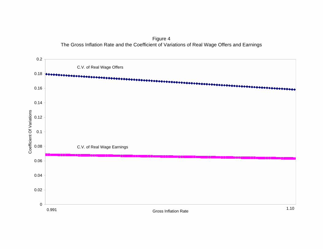
Figure 4The Gross Inflation Rate and the Coefficient of Variations of Real Wage Offers and Earnings

0

0.02

0.04

0.06

0.08

0.1

0.12

0.14

0.16

0.18

0.2

Gross Inflation Rate

Coe

ffici

ent O

f Var

iatio

ns

C.V. of Real Wage Earnings

C.V. of Real Wage Offers

0.991 1.10

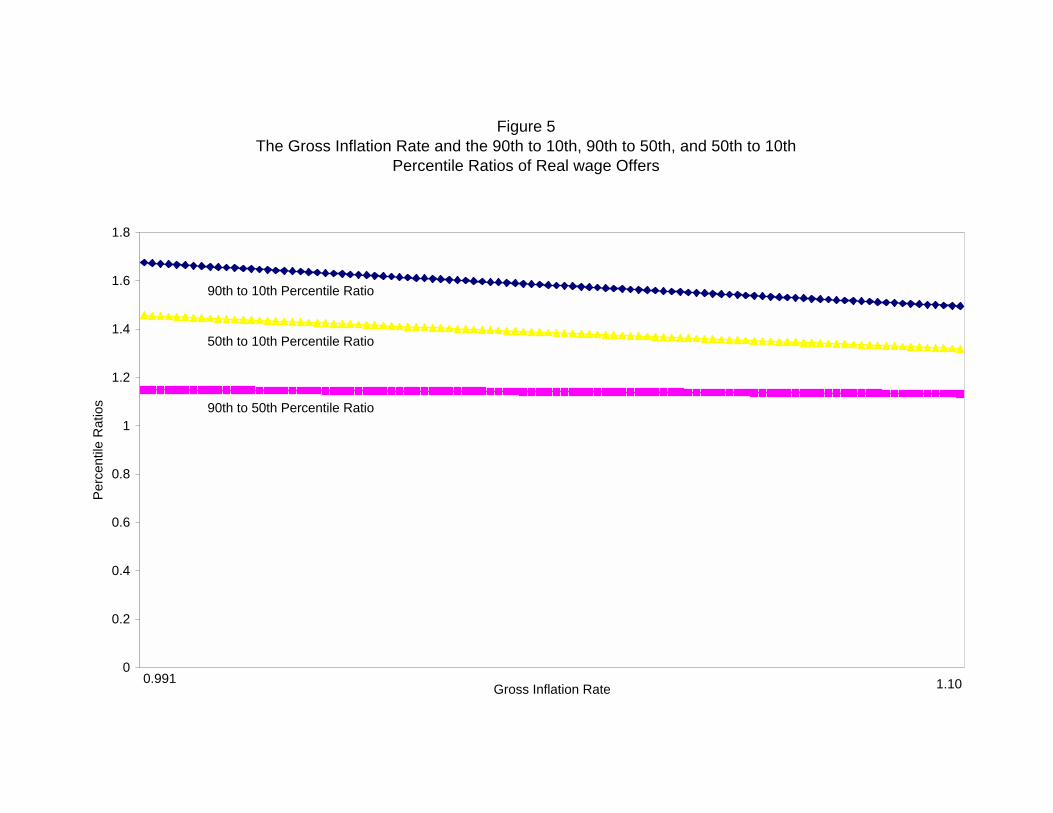
Figure 5The Gross Inflation Rate and the 90th to 10th, 90th to 50th, and 50th to 10th

Percentile Ratios of Real wage Offers

0

0.2

0.4

0.6

0.8

1

1.2

1.4

1.6

1.8

Gross Inflation Rate

Perc

entil

e R

atio

s 90th to 50th Percentile Ratio

50th to 10th Percentile Ratio

90th to 10th Percentile Ratio

0.991 1.10

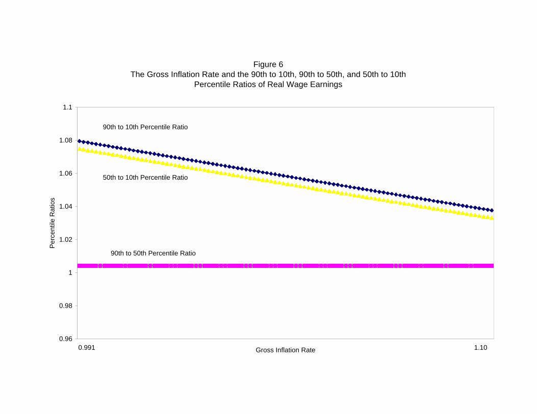
Figure 6The Gross Inflation Rate and the 90th to 10th, 90th to 50th, and 50th to 10th

Percentile Ratios of Real Wage Earnings

0.96

0.98

1

1.02

1.04

1.06

1.08

1.1

Gross Inflation Rate

Perc

entil

e R

atio

s

0.991 1.10

90th to 50th Percentile Ratio

50th to 10th Percentile Ratio

90th to 10th Percentile Ratio

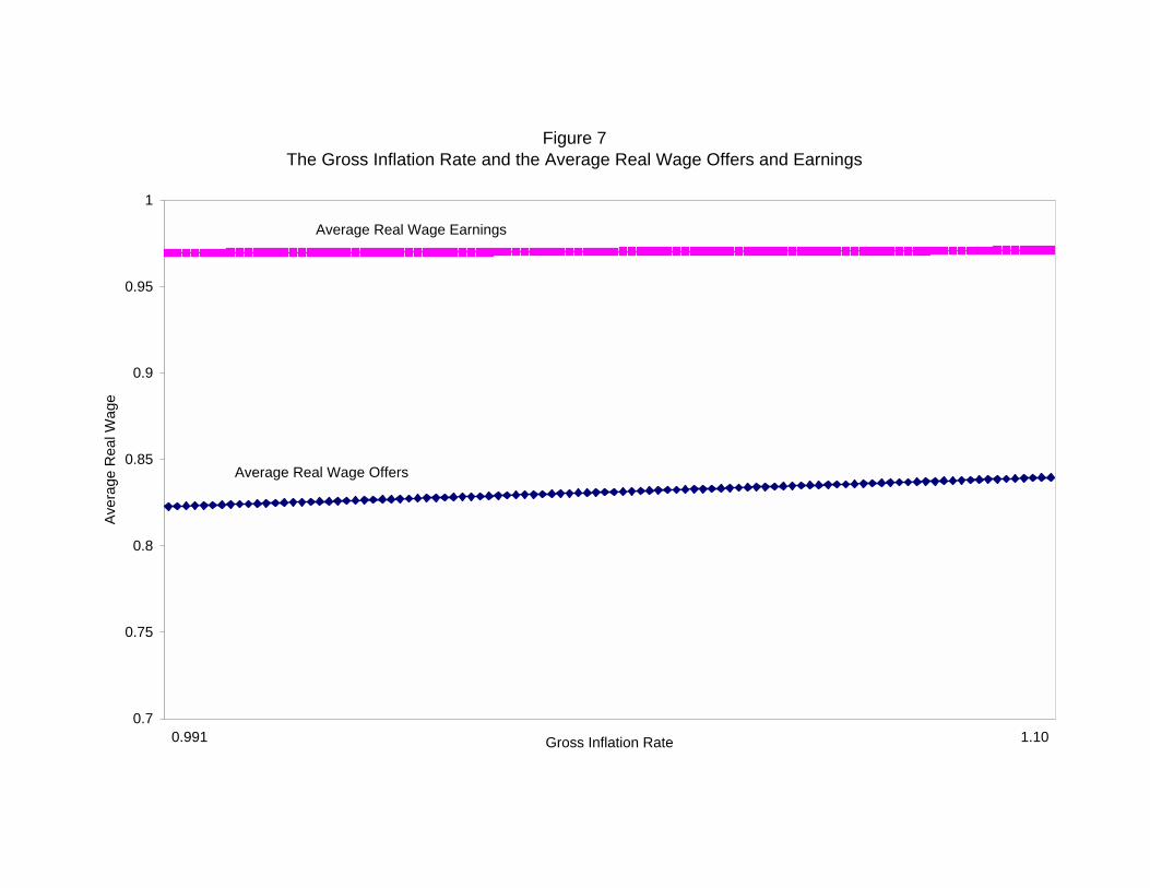
Figure 7The Gross Inflation Rate and the Average Real Wage Offers and Earnings

0.7

0.75

0.8

0.85

0.9

0.95

1

Gross Inflation Rate

Aver

age

Rea

l Wag

e

Average Real Wage Earnings

Average Real Wage Offers

0.991 1.10