incentives, risk, and the role of private investments in

Louisiana State UniversityLSU Digital Commons

LSU Doctoral Dissertations Graduate School

2010

Incentives, risk, and the role of private investmentsin Louisiana coastal wetland restorationcheikhna Ould DedahLouisiana State University and Agricultural and Mechanical College

Follow this and additional works at: https://digitalcommons.lsu.edu/gradschool_dissertations

Part of the Agricultural Economics Commons

This Dissertation is brought to you for free and open access by the Graduate School at LSU Digital Commons. It has been accepted for inclusion inLSU Doctoral Dissertations by an authorized graduate school editor of LSU Digital Commons. For more information, please [email protected].

Recommended CitationOuld Dedah, cheikhna, "Incentives, risk, and the role of private investments in Louisiana coastal wetland restoration" (2010). LSUDoctoral Dissertations. 2309.https://digitalcommons.lsu.edu/gradschool_dissertations/2309

https://digitalcommons.lsu.edu?utm_source=digitalcommons.lsu.edu%2Fgradschool_dissertations%2F2309&utm_medium=PDF&utm_campaign=PDFCoverPages

https://digitalcommons.lsu.edu/gradschool_dissertations?utm_source=digitalcommons.lsu.edu%2Fgradschool_dissertations%2F2309&utm_medium=PDF&utm_campaign=PDFCoverPages

https://digitalcommons.lsu.edu/gradschool?utm_source=digitalcommons.lsu.edu%2Fgradschool_dissertations%2F2309&utm_medium=PDF&utm_campaign=PDFCoverPages

https://digitalcommons.lsu.edu/gradschool_dissertations?utm_source=digitalcommons.lsu.edu%2Fgradschool_dissertations%2F2309&utm_medium=PDF&utm_campaign=PDFCoverPages

http://network.bepress.com/hgg/discipline/1225?utm_source=digitalcommons.lsu.edu%2Fgradschool_dissertations%2F2309&utm_medium=PDF&utm_campaign=PDFCoverPages

https://digitalcommons.lsu.edu/gradschool_dissertations/2309?utm_source=digitalcommons.lsu.edu%2Fgradschool_dissertations%2F2309&utm_medium=PDF&utm_campaign=PDFCoverPages

mailto:[email protected]

INCENTIVES, RISK, AND THE ROLE OF PRIVATE INVESTMENTS IN

LOUISIANA COASTAL WETLAND RESTORATION

A Dissertation

Submitted to the Graduate Faculty of the Louisiana State University and

Agricultural and Mechanical College in partial fulfillment of the

requirements for the degree of

Doctor of Philosophy

in

The Department of Agricultural Economics & Agribusiness

by Cheikhna Ould Dedah

B.S., Nouakchott University, 2000 M.S., Louisiana State University, 2005 M.S., Louisiana State University, 2007

December 2010

ii

DEDICATION

I dedicate this humble work to:

My mother, Faitma, and my grandmother, Eye, ……………

In remembrance of my father who passed away…………….

iii

ACKNOWLEGEMENTS

First of all, I want to very kindly and humbly thank my advisor, Professor Richard F.

Kazmierczak, Jr., who exemplifies an outstanding advisor model that I will strive to imitate in

the future as my career progresses. Dr. Kazmierczak is an excellent writer, detail oriented, and

insightful advisor with a unique way of interacting with and developing students to be better

thinkers and researchers. I am very fortunate to have the opportunity to work under his

direction, and I thank him dearly for his help and kindness. Without his help and

encouragement, this research would not be possible.

I wish also to express my sincere appreciation to Dr. Walter R. Keithly, Jr., for his

help facilitating the collection of the survey data and his help with drafting the survey

questionnaire. I also want to thank all my other committee members for their valuable

contribution to this research: Dr. Jeffrey M. Gillespie. Dr. Rex H. Caffey, and Dr. John V.

Westra for their valuable contributions to this research. I want to thank Ms. Huizhen Niu for

teaching me how to use GIS and helping me with the mapping of the properties of the

landowners. I would like to thank Ms. Debbie Mosher, and all my follow graduate students

for helping me process and mail my survey questionnaires.

Funding for this research was provided by the United States Environmental and

Protection Agency (EPA), and Louisiana‟s Coastal Restoration and Enhancement trough

Science and Technology (CREST) program. Many thanks indeed for the financial support.

iv

Finally, I cannot be grateful enough to thank my mother, Faitma Bint Cheikh, and my

Grandmother Eye, and my wonderful, and caring brother Sidina Dedah, and all my brothers

and sisters for unconditional support they have given me. Without you, I will not achieve this

success. My limited English words fail short to describe how grateful and thankful I am to

your support and patience ….…..I love you all dearly!!

v

TABLE OF CONTENTS

ACKNOWLEGEMENTS .............................................................................................................. iii

LIST OF TABLES ....................................................................................................................... vii

LIST OF FIGURES ...................................................................................................................... viii

ABSTRACT ................................................................................................................................... ix

CHAPTER 1. INTRODUCTION.................................................................................................... 1 1.1. Problem Statement.................................................................................................................... 2 1.2. Justification............................................................................................................................... 3

1.3. Objectives ................................................................................................................................. 5

CHAPTER 2. LITERATURE REVIEW......................................................................................... 7 2.1. General Factors Affecting Investment Decisions ..................................................................... 7 2.2. Risk Aversion and Investment Decisions ............................................................................... 13

2.3. Option Values and Investment Decisions............................................................................... 18

CHAPTER 3.THEORETICAL ANALYSIS................................................................................. 23 3.1. Investment under Certainty: Net Present Value (NPV) Approach ........................................ 23 3.2. Investment under Uncertainty ................................................................................................ 26

3.2.1. The Role of Risk Aversion ............................................................................................ 27 3.2.2. The Value of Information(Option Value Approach)...................................................... 31

3.2.3. Implications for a Potential Wetland Restoration Policy .............................................. 34 CHAPTER 4. EMPIRICAL ANALYSIS...................................................................................... 39

4.1. The Tobit Model ..................................................................................................................... 41 4.2. The Double Hurdle Model...................................................................................................... 45

4.3. Hetroskedasticity and Non-normality..................................................................................... 49 CHAPTER 5. SURVEY DESIGN AND DATA SUMMARY..................................................... 52

5.1. Survey Design and Response ................................................................................................. 52 5.2. Risk Elicitation Methods ....................................................................................................... 57

5.2.1. Self Ranking Risk Method .......................................................................................... 57 5.2.2. Multi- item Scale Approach .......................................................................................... 58 5.2.3. Investment Method ...................................................................................................... 59

5.3. Descriptive Summary of Survey Results................................................................................ 61 5.3.1. Demographics .............................................................................................................. 61

5.3.2. Attitudes toward Wetland Conservation and Various Incentive Programs .................. 63 5.3.3. Characteristics of the Properties .................................................................................. 65

vi

5.3.4. Wetland Investment ..................................................................................................... 69 5.3.5. Landowners‟ Risk Preferences .................................................................................... 73

CHAPTER 6. RESULTS OF EMPIRICAL ESTIMATION ....................................................... 80 6.1. Data Summary ........................................................................................................................ 80 6.1.1. Characteristics of Landholdings ...................................................................................... 82

6.1.2. Characteristics of the Landowners .................................................................................... 84 6.1.3. Influence of Government Programs .................................................................................. 85

6.2. Results of the Tobit Model .................................................................................................... 85 6.3. Results of the Double Hurdle Model ..................................................................................... 92 6.4. Model Selection .................................................................................................................... 105

CHAPTER 7. CONCLUSIONS AND POLICY IMPLICATIONS............................................ 108

REFERENCES ............................................................................................................................ 116

APPENDIX-A. WETLAND INVESTMENT SURVEY QUESTIONNAIRE........................... 124

APPENDIX-B. RESULTS OF THE AUXILIARY REGRESSION MODEL ........................... 133 APPENDIX-C. RESULTS OF THE RESTRICTED TOBIT MODEL ...................................... 134

VITA............................................................................................................................................ 135

vii

LIST OF TABLES

Table 5.1: Statements Used to Elicit the Landowners‟ Risk preference ....................................... 60

Table 5.2: An Example of the Basic Structure of the Investment Method Experiment Using a $25,000 Investment Level ............................................................................................................ 61

Table5.3: Demographic Characteristics of the Respondents ........................................................ 62

Table5. 4: Statistical Summary of the Property Characteristics for Respondents to the Landowner Survey. .................................................................................. 66

Table 5.5: Ownership Structure and Land Management .............................................................. 66

Table 5.6: Statistical Summary of Continuous Variables in the Investment Section ................... 70 Table 5.7: Type of Wetland Restoration Practices that the Respondents Used ........................... 70

Table 5.8. Variance Matrix of the Principal Component Analysis ............................................... 75

Table 5.9. Factor Loading Matrix of the Principal Component Analysis .................................... 76

Table 5.10: Landowners‟ Risk Attitudes Based on the Multi- item Scale Approach ..................... 77

Table 5.11: Landowners‟ Investment Distribution Choices Associated with a $25,000 Investment Level ........................................................................................................ 77

Table 6.1: Summary Statistics for the Variables Used in the Analysis ......................................... 81

Table 6.2: Parameter Estimates of the Tobit Model ..................................................................... 87 Table 6.3. Marginal Effects for the Tobit model .......................................................................... 88

Table 6.4. Parameter Estimates of the Double Hurdle Model....................................................... 94

Table 6.5. Marginal Effects for the Double Hurdle Model ........................................................... 96

viii

LIST OF FIGURES

Figure 5.1: An Aerial Photography Map of a Sample Wetland Tract ........................................... 56

Figure 5.2: Distribution of the Survey Respondents across Louisiana‟s Coastal zone ................. 58

Figure 5.3: Respondents‟ Attitudes toward Wetland Conservation .............................................. 64

Figure 5.4: Landowners‟ Preferences for Various Incentive Instruments for Wetland Restoration and Maintenance in Coastal Louisiana. ..................................................................... 65

Figure 5.5: Values Assigned by the Landowners to Various Land Uses Activities Associated with the Current Use of the Property Tract ................................................................................... 68

Figure 5.6: Respondents‟ Perceptions about Various Factors That Influence Their Decisions to Invest in Wetland Restoration and Maintenance....................................................................... 71

Figure 5.7: Respondents‟ Perceptions about Various Factors that Influence Their Decisions

not to Invest in Wetland Restoration and Maintenance................................................................. 72 Figure5.8: Respondents‟ Perceptions about Uncertainty Sources................................................. 73

Figure5.9: Landowners‟ Risk Attitude Scores Based on the Self Ranking Question ................... 74

Figure6.1 Predicted Wetland Investments Associated with Various Levels of Risk Attitudes .. 100

Figure 6.2: Histogram of Predicted Probability of no Investment in Wetland Restoration and Maintenance ................................................................................................................................ 103

Figure 6.3: Histogram of Predicted Probability of Investment in Wetland Restoration and Maintenance ............................................................................................................................... 104

ix

ABSTRACT

The coast of Louisiana, with more than three million wetland acres, accounts for about

40 percent of the nation‟s total wetlands. Louisiana is estimated to have lost more than 1.2

million acres of its coastal wetland in the last century. Although 75% of Louisiana‟s coastal

wetlands are privately owned, little has been done to encourage private landowners to

undertake wetland restoration projects. This dissertation examines the factors that influence

the decisions of the landowners to undertake wetland restoration projects. We develop a

theoretical framework for understanding the landowner‟s decision-making process in the

presence of high uncertainty and increasing restoration costs. The condition under which

landowners will invest in wetland restoration and maintenance is derived under the

assumptions of risk aversion and relatively high restoration costs. The validity of the

theoretical model is tested using data from a mail survey of private wetland landowners in

coastal Louisiana that was conducted in Fall of 2009. Two econometric (Tobit and double

hurdle) models are estimated to determine the importance of various factors including risk

aversion on the probability and the level of private coastal wetland investments.

The Likelihood ratio (LR) test shows that the double hurdle model statistically

outperforms the Tobit model. The results suggest that the decision to invest in wetland

restoration and how much to invest appear to be determined by different processes. The

results of the double hurdle model show that risk plays an important role in landowners‟

decisions to invest in wetland restoration and maintenance activities. Landowners who are

risk averse make less investment in wetland restoration and maintenance projects than other

landowners, and landowners who own properties that are located in risk prone areas are less

likely to invest in wetland restoration than other landowners. In addition, the results show that

x

landowners‟ attitudes toward conservation, income related to the property, participation in

government wetland programs, ownership structure, and wetland property size are all

important determinants of the landowners‟ investment decisions. The analysis emphasizes the

need to incorporate risk into the design of wetland incentive programs to encourage private

landowners to undertake wetland restoration projects in coastal Louisiana.

1

CHAPTER 1

INTRODUCTION

The coast of Louisiana, with more than three million wetland acres, accounts for about

40 percent of the nation‟s coastal wetlands (Lipton et al., 1995). In the last century, however,

Louisiana is estimated to have lost more than 1.2 million acres (1,875 square miles) of its

coastal wetlands (CWPPRA 2006). A number of factors have contributed to this loss. Topping

the list is the construction of flood-control levees along the Mississippi River (Boesch et al.

1994) which prevent wetlands from receiving adequate fresh water and nutrients that are

necessary to their survival. In addition, the dredging of access canals and navigation channels

led to the redirection of alluvial sediments away from the coast which has exacerbated erosion

and saltwater intrusion. As a result, it is estimated that about 160-200 million metric tons per

year of sediments that once supplied the coastal wetlands are now delivered directly onto the

outer continental shelf (Caffey and Shexnayder 2003; Caffey, 2005). Besides these human-

induced factors, wetland losses are also caused by natural factors such as hurricanes, sea level

rise, land subsidence, and nutria herbivory activities. For example, the U.S. Geological

Survey estimates that 219 square miles of Louisiana coastal wetlands were destroyed as a

result of Hurricanes Katrina and Rita (Barras et al., 2008). According to some estimates, the

economic cost of projected wetland loss from all sources by 2050 under a “no action”

scenario is in the range of $27-$100 billion (LADNR 1999).

In an effort to address the problem of Louisiana‟s coastal land loss, the U.S. Congress

passed the Coastal Wetlands Planning, Protection and Restoration Act (CWPPRA) in 1990.

But, given the estimated price tag for coastal restoration of $20 billion (Galloway et al.,

2009), only a fraction of the needed funds have been allocated, with CWPPRA, the largest

program, accounting for only $60 million annually. Several other public restoration projects

2

in the coastal zone of Louisiana have been funded by programs such as the Coastal Impact

Assistance Program (CIAP), the Louisiana Coastal Area (LCA) program, the Coastal Wetland

Reserve Program (CWRP), the Chrismas Tree Projects Program, and the Vegetation Planting

Program initiated under the Louisiana‟s Coastal Wetlands Conservation Plan. CWRP,

introduced to restore coastal wetlands on areas previously converted to agriculture, has

succeeded in restoring hundreds of acres of coastal wetlands (CPRA, 2007). However, the

limited availability of public funding, along with the magnitude of the problem, increases the

importance of finding alternative approaches to addressing the issue of wetland loss in coastal

Louisiana. Given that the vast majority of wetland properties are privately owned, incentive-

based mechanisms to encourage private actions may be an appealing alternative approach.

Encouraging landowners to undertake private restoration and maintenance activities

can be a difficult task for several reasons. First, the decision to invest in wetland restoration

and maintenance is subject to a high level of uncertainty associated with future climate

change, changes in restoration technologies, and changes in wetland regulatory policy.

Second, the majority of benefits associated with wetland restoration and maintenance

activities accrue to the public rather than to private landowners. Other reasons that may

prevent private investment include diminishing surface and sub-surface incomes, increasing

regulatory constraints, and a current property tax policy that fails to account for the use value

for the wetland property (Caffey et al., 2003).

1.1 Problem Statement

Louisiana is projected to lose an additional 431,000 acres (673 square miles) of its

coastal wetlands by the year 2050 if the current wetland loss rates continue (CWPPRA 2006).

3

The economic implications of this projected loss are often debated, but there are billions of

dollars that are directly or indirectly derived from activities occurring on these wetlands.

Although 75% of these wetlands are privately owned Caffey et al., 2003), little is known

about how much private investment has been allocated to restoration and maintenance, nor is

there a good understanding of what can be done to encourage private landowners to maintain

and protect their coastal lands. This dissertation seeks to fill this information void by

estimating the amount of private investment (at least for a subset of landowners) and

investigating the factors that influence private Louisiana landowners to invest in coastal

wetland restoration and maintenance activities, with particular emphasis on the influence of

risk aversion and public subsidy programs on the private investment decision. More

specifically, the following questions are addressed in this dissertation: First, what are the

factors that motivate a landowner to undertake wetland restoration and maintenance

activities? Second, what are the factors that deter a landowner from investing in wetland

restoration and maintenance activities? Third, how does uncertainty influence a landowner‟s

decision making process? And finally, how do potential government subsidy programs

influence the landowner‟s investment decision?

1.2. Justification

Given that 75% of the wetland acreage in Louisiana‟s coastal zone is privately owned,

successful coastal wetland restoration efforts will at least partly depend on the decisions of the

private landowners who hold the ownership rights. Little or no effort, however, has been

employed to encourage private wetland landowners to undertake wetland restoration projects

in coastal Louisiana. The majority of wetland restoration projects in the coastal zone are still

addressed through public programs such as the Coastal Wetlands Planning, Protection and

4

Restoration Act (CWPPRA). These public programs, which generally fail to engage the

landowners in the restoration process lack the monetary resources to adequately address all of

the wetland loss problems in the coastal zone. Even if additional government funding was to

be secured, the cost effectiveness of these public restoration projects by CWPPRA and other

public programs remains an issue of debate. At the same time, several factors have been

proposed as reasons for the lack of private investment by landowners, including increasing

investment risk, diminishing surface and sub-surface incomes, increasing regulatory

constraints, and the public nature of the majority of the benefits of private restoration projects.

Given these problems, there has been a call for the use of incentive based voluntary programs

to encourage the landowners to invest in wetland restoration and maintenance activities.

In this dissertation, I investigate the factors that influence the landowners to undertake

wetland restoration projects in coastal Louisiana. Understanding these factors is important for

the design and implementation of voluntary programs to encourage private investment. For

example, an estimated empirical model of landowner investment decision making can be used

to provide information about the expected probability of participation, the expected level of

investment, and the characteristics of the landowners who are most likely to participate. This

information can provide the policy decision makers with the information needed to design

wetland incentive programs that are both more cost effective and have higher participation

rates than nontargeted wetland incentive programs. In addition, the information provided by

an empirical model may allow policy makers to design incentive programs targeting

restoration projects in areas that are most affected by wetland losses. This information is

important when policy makers have to prioritize among competing wetland restoration

projects given limited funding resources.

5

1.3 Objectives

The overall objective of this dissertation is to investigate the factors that influence

landowners‟ decisions to invest in coastal wetland restoration and maintenance when these

decisions are made in the presence of uncertainty and fixed costs. Specific objectives inc lude:

1. Develop a theoretical model of the landowners‟ decision-making process in the face of

uncertainty and fixed costs;

2. Determine the characteristics of wetland landowners in coastal Louisiana, including

their risk preferences, attitudes toward private restoration and maintenance, the actual

use of their properties, attitudes toward various government incentive programs, and

their general socioeconomic profile;

3. Empirically estimate the importance of risk aversion, public subsidy programs, and

other factors affecting landowner decisions to invest in coastal wetland restoration and

maintenance projects; and

4. Examine the policy implications of the study results and devise policy

recommendations that address the desirability and potential magnitude of private

landowner investment in restoring and maintaining coastal Louisiana wetlands.

The remainder of the dissertation is organized as follows. Chapter 2 examines the

economic and investment literature that relates to restoration-type decision making, including

the potential roles of general factors, risk aversion, and option values. Chapter 3 takes this

literature base and develops a theoretical model of the private wetland restoration decision

making process and draws some tentative implications from the model structure. Chapter 4

6

presents the empirical model. Chapter 5 then presents the design of the survey questionnaire

used to collect data and summarizes the information reported by respondents.. Chapter 6

presents the results of the model estimation, with Chapter 7 summarizing the main findings

and discussing the potential policy implications.

7

CHAPTER 2

LITERATURE REVIEW

Although there have been a number of studies that have identified factors that are

important to private landowners‟ investment decisions concerning other activities, private

investment in coastal wetland restoration and maintenance has not been seriously studied to

date. A review of these studies is presented in this chapter, beginning with a set of studies that

looked at factors that influence investment decisions under the assumption of risk neutrality.

The second section presents the results of empirical studies concerning the effect of risk

aversion on investment decisions, while the third section examines the results of empirical

studies on the role of option values in investment decisions.

2.1 General Factors Affecting Investment Decisions

Even though there are no studies that specifically examined those factors influencing

decisions to privately invest in wetland restoration and maintenance in coastal Louisiana,

there are a number that have identified general factors that may be important to wetland

conservation efforts in the U.S. and other countries, including the factors influencing

participation in publicly- financed wetland restoration programs. Jones et al. (1995) surveyed

private landowners in New Zealand to determine their attitudes toward wetland protection and

potential conservation mechanisms. The survey results showed that the majority of private

landowners placed importance on the role of wetlands in maintaining water quality and

providing species habitat. With regard to landowner preferences toward various conservation

instruments, the survey revealed that incentive and voluntary instruments were most

preferred. One of the authors‟ conclusion from this result was that conservation programs

8

should use a range of land-use planning mechanisms, including ones based on economic

incentives and financial compensation. Simple correlation tests showed that property size and

the proportion of income derived from the property were significantly related to the

landowners‟ attitudes about the importance and appropriate use of wetland areas. In addition,

landowners who were engaged in farming activities were found to have negative attitudes

toward the protection of wetlands.

Parks and Kramer (1995) investigated farmer participation in wetland restoration

programs in the United States. Results from logit analysis showed that increases in

agricultural benefits decreased the probability of participation in wetland restoration. Farmer

knowledge of government programs and their potential benefits, as measured by government

payments received per acre, were also found to significantly (at the 10% level) increase the

probability of participating. Age and ownership structure were important factors in the

participation decision as well, with older farmers and owner operators being more likely to

become involved in wetland restoration programs. The authors also examined the probability

of participation by county and used this information to calculate the expected acreage restored

and the expected government costs for the restoration.

From an international perspective, Soderqvist (2003) used a random sample of 200

Swedish farmers to determine the factors that influence their willingness to participate in a

catchment-based program for wetland creation in Sweden. The results of a probit analysis

showed that factors such as age, attitudes of farmers, and perceived advantages and

disadvantages of the program were important determinants of participation decisions. The

study concluded that financial factors (i.e., subsidies) were not the sole determinant of a

farmer ‟s willingness to participate in the program, as various private and public

9

environmental benefits of the program were also significantly related to participation

decisions.

Aside from the above studies that focused on wetlands, other studies have examined private

landowner investment decisions concerning other activities. For example, Ervin and Ervin

(1982) examined the factors that determine the use of soil conservation practices using a

random sample of Missouri farmers. The study found that education, perception of the degree

of erosion problem, the susceptibility of soil to erosion, and cost sharing subsidies were

positively correlated with the farmers‟ soil conservation efforts. However, when the number

of soil practices was used as a dependent variable, only education, perception of the degree of

erosion problem, farm type, and risk aversion were statistically significant in their model. The

number of practices used was negatively related to the risk aversion of the farmers, and

positively related to education and the perception of erosion problem. Similarly, Norris and

Batie (1987) used a Tobit model to investigate the soil conservation decisions among Virginia

farmers. Using total conservation expenditures as a dependent variable, the study found that

financial factors - such as income and debt level - are the most important determinants of a

farmer ‟s investment decision. Income had a positive influence on the level of conservation

expenditures, and debt level had a negative influence on the level of conservation

expenditures. Other factors, such as perception of erosion, farm size, education, off- farm

employment, tenure arrangement, tobacco acreage, and the existence of conservation plan

were also important factors in the decision to invest. More specifically, farm size and

education were positively related to the level of conservation investment while tenure

arrangement was negatively related to the level of conservation investment.

10

Featherstone and Goodwin (1993) analyzed the factors that influenced Kansas farmers

to invest in long-term conservation improvements. Employing a Tobit analysis, the authors

showed that farm characteristics - such as farm size, debt, erosion level, type of farm, and

participation in government programs - were important explanatory factors. In particular, the

larger the farm size is and the larger the government payments, the higher the likelihood of

participation and the higher the level of investment that would be made. The authors also

found that operator and farm characteristics, such as age and ownership type, had significant

influences on conservation expenditures. More specifically, the older the farm operator is, the

less likely an expenditure would be made and, if made, the smaller the investment that would

be undertaken. At least in Kansas, farms organized as corporations made larger investments

than sole-owner farms. Unlike Norris and Batie (1987), income was not found to significantly

influence overall conservation expenditures. In another study examining the role of

ownership, Soule et al. (2000) used a logit model to estimate the influence of land tenure on

the adoption of conservation practices by U.S. corn producers. The authors extended previous

analyses by distinguishing renters based on lease type and by distinguishing conservation

practices based on the timing of costs and returns. The results of their long-run conservation

tillage model revealed that adoption was significantly and positively associated with farm

size, education, the proportion of the farm in corn and soybeans, and the susceptibility of the

land to erosion, and negatively related to age. Tenure and participation in government

programs were not significant factors in the conservation tillage model. The authors‟ medium-

term practices model showed similar results to the conservation tillage model, with the

exception that the coefficient on tenure was negative and statistically significant. Overall,

study results suggested that cash-renters were less likely to adopt conservation tillage than

11

owner-operators, and share renters were less likely than owner-operator to adopt medium-

term practices. In an international context, Layva et al. (2007) analyzed the adoption of soil

conservation practices among 223 olive tree farmers in Spain. Three probit models were

estimated for the three different conservation practices (tillage, terraces with stonewalls, and

non-tillage practices). The study found that farm profitability, age of the farm operator, and

the probability of passing on the farm to a relative were the most important determinants of

the farmer‟s adoption decision.

Similar to the agricultural examples, a number of factors have been identified as

important in forestry management investment decisions. Alig (1986) and Straka et al. (1984)

found a significant positive relationship between household income and forestry investment.

Later, however, Kline et al. (2000) found the relationship between income and forestry

investment to be negative. Romm et al. (1987) used a logit regression to determine the

factors that influence private forestry investment in northern California. The results of the

study confirmed that income, age, and full time residency were the most significant factors in

explaining forestry investment. More specifically, high income and full time residency were

positively related to forestry investment, but absentee ownership, middle-ranged incomes, and

old age were negatively related to the forestry investment. Property size was found to be an

important factor in explaining investment in timber harvesting, but not in general forestry

management. Nagubadi et al. (1996) used a probit model to analyze the participation of

nonindustrial forest landowners in government forestry programs. The study found that

property size, ownership reasons, government sources of information, and membership in

forestry organizations were the most important determinants of program participation. Age,

12

risks associated with the loss of property rights, and years of ownership were also important

factors.

In considering the interactions between public and private decision making, Zhang and

Flick (2001) examined the influence of environmental regulations (i.e., Endangered Species

Act) and public financial assistance programs on private reforestation behavior. A two-step

selection model was employed in the analysis. First, a probit model was used to estimate

reforestation decisions. Second, the residuals from this model were retained and a selection

model was estimated for the landowners who had replanted by using the level of investment

as a dependent variable. The results of the probit model showed that the probability of

reforestation investment was positively related to technical assistance and awareness of cost-

share program, but negatively related to the distance from known endangered species habitats.

None of the demographic variables, such as income or age, were found to be important factors

in the reforestation decisions. The results of the selection model showed that the level of

investment is positively related to the use of reforestation tax incentives and negatively related

to the use of cost-share subsidies. The later implies a substitution effect between public and

private capital. In addition, landowner characteristics such as income, age, and knowledge of

forestry influenced the decisions about the level of reforestation investment. Income and

knowledge of forestry were positively related to the level of investment, but age was

negatively related to the level of investment. Property size was not a significant factor in

either the probit or selection models.

In a more recent study, Dhakal et al. (2008) investigated the factors that influence the

decision of small landowners to invest in forestry plantations in New Zealand. Using a

double hurdle model, the authors found that property size, ownership type, period of

13

landholding, land use in dairy production, experience in grain farming, perception about

forestry tax policy, expectation about future log prices, and percentage of off- farm income

were the most important predictors of the decision to undertake forestry plantation

investments. In addition, the study found that property size, perception about forestry tax

policy, expectation about future log prices, location of the land, and area used in sheep and

beef production were strong determinants in the decision about the extent of forestry

plantation investment. Thus, unlike Zhang and Flick (2001), property size was important in

both the decision to invest and the level of investment undertaken. Property size was

positively related to the probability of investing, but negatively related to the extent of

investment.

2.2 Risk Aversion and Investment Decisions

The majority of the empirical studies summarized in the previous section (with the

exception of Ervin and Ervin 1982) relied on the assumption that all decision makers are risk

neutral even though it is likely that this assumption does not match reality. In the context of

wetland restoration and maintenance, landowners face substantial levels of uncertainty about

how future climatic, economic, and institutional factors will affect the payoffs from their

investments. As a result, it is likely that risk aversion plays an important role in a landowner ‟s

investment decision. The potential impact of risk aversion on investment decisions in the

presence of uncertainty has been empirically explored using a variety of frameworks,

including the expected utility framework (Koundouri et al. 2006; Kim and Chavas 2003;

Antle 1983) and stochastic dominance analysis (Goldstein et al. 2006; Benitez et al. 2006.

This section presents a summary of the main findings of these studies and discusses the

econometric modeling techniques used in the applications.

14

Stordal et al. (2007) applied stochastic efficiency with respect to a function (SERF) to

analyze the impact of risk aversion on the optimal tree replanting decision. Risk aversion was

profoundly influential in determining the certainty equivalence for all rotation strategies

considered. Specifically, the results showed that certainty equivalence was a decreasing

function of the risk aversion of owners. The results also indicated that risk-averse forest

owners chose a higher optimal age of replacement of trees than risk neutral landowners.

Hence, risk aversion influenced both the optimal tree replacement strategy and the

reinvestment decision. The authors concluded that risk aversion needs to be considered when

designing policy measures to influence forestry investments.

Goldstein et al. (2006) used stochastic dominance (SD) analysis to identify specific

Koa forestry business strategies that were associated with risk-efficient land-use options in

Hawaii. The study designed a set of hypothetical business strategies based on income from

timber harvest, two existing government conservation programs, integrated cattle grazing, and

selling carbon offset credits. The results of the analysis were based on cumulative net present

value (NPV) distribution functions of the land-use business strategies generated from Monte

Carlo simulation, and they showed that business strategies in which the landowners receive

rental payment plus cost-share assistance were the most efficient. This implies that programs

like the Conservation Reserve Enhancement Program (CREP) – in which the landowners

received payment and cost share subsidies – could create viable business strategies for risk-

averse landowners in Hawaii. Benitez et al. (2006) also used stochastic dominance (SD)

analysis, but in this case to study land allocation problems under risk for shaded coffee

production in the Choco region of West Ecuador. Study results indicated that shaded coffee is

not a risk efficient land use, regardless of the degree of diversification. Hence, conservation

15

payments required for preserving shaded coffee would need to be much higher than

conservation payments calculated under risk neutrality assumptions. These results stressed the

need for considering risk aversion factors when implementing conservation policy

instruments.

In another international context, Hagos and Holden (2006) studied the influence of

risk aversion, land tenure, public programs, and resource poverty on soil conservation

investment decisions in northern Ethiopia. The study measured the risk preferences of

households using hypothetical questions based on a utility function with constant partial risk

aversion. A Probit model was then used to model the factors that influence the decisions to

invest in soil conservation, with a subsequent Tobit model employed to model the factors that

influence the intensity of investment. The authors found that risk aversion played an

important role in a household‟s decision to intensify soil conservation measures but not in the

decision to use soil conservation measures. Risk aversion was negatively correlated with the

level of investment made in soil conservation. In addition, the study revealed that public

conservation programs had a positive influence on private investment. Other factors,

including land characteristics and the perception of returns on conservation investments, were

found to be important in a household‟s decision to invest and intensify soil conservation.

Among the various variables included in of the analyses of technology adoption, risk

has been recognized as a major factor in the adoption decision (Feder, Just, and Zilberman

1985). Saha et al.(1994) developed an empirical and analytical framework for divisible

technology adoption under incomplete information diffusion and output uncertainty. The

analytical framework showed that neither risk aversion of the producers, nor their risk

perceptions, should play a role in the adoption decision. These risk factors, however, should

16

play an important role in the degree of adoption if the producers decided to adopt the

technology. Koundouri et al. (2006) extended the theoretical framework of Saha el al. (1994)

to allow risk aversion and uncertainty to influence the technology adoption decision. The

model was empirically tested using survey data of irrigation technology adoption practices by

265 Greece farmers. Using the first four moments of the profit distribution to approximate

production risk in a logit model, the study found that risk influenced the farmer ‟s decision to

adopt the new irrigation technology. Specifically, farmers who faced more production risk

were more likely to adopt new irrigation technology, suggesting that farmers chose to adopt

new technology in order to hedge against production risk. In addition, the study found that

farmers value the prospects of receiving new information to use in their adoption decision

making. In a more recent paper, Torkamani and Shajari (2008) applied a logit model to

investigate factors affecting adoption of new irrigation technologies by wheat farmers in three

major Iranian districts. The study used a moment based approach to estimate the risk premium

associated with water use, which was then used to estimate the risk attitudes of the farmers.

Assuming that the risk preferences of the farmers exhibited constant relative risk aversion, the

results showed that the risk attitudes of farmers have positive and significant effects on the

decision to adopt new irrigation technologies. As a result, risk averse farmers were more

likely to adopt new irrigation technologies that allowed them to save water and reduce

production risk during the times of water shortage. Beside the risk aversion factor, the study

found that location, debt level, education, and age were important determinants in the decision

to adopt new irrigation technologies. Education had a positive effect on the probability of

adoption and age had a negative effect on the probability of adoption. Not surprisingly, farms

located in arid areas were more likely to adopt new water irrigation technologies.

17

Using as somewhat different approach, Isik and Khanna (2003) employed a nonlinear

mean-standard deviation expected utility function to determine the impacts of risk aversion

and uncertainty about weather and soil conditions on the decision to adopt site-specific

technologies and the levels of cost-share subsidies required to induce adoption. The study

found that uncertainty and risk-aversion had negative impacts on adoption decisions such that

ignoring risk aversion and uncertainty would overestimate the economic and environmental

benefits of site specific technologies and underestimate the subsidy level required to

encourage adoption. Abadi Ghadim et al. (2005) analyzed the importance of uncertainty and

risk aversion in decisions to adopt crop innovation in Western Australia. Farmers were

interviewed over a three-year span to elicit their risk preferences and risk perceptions

concerning a new crop technology for the area (chickpeas). In the survey, farmers were asked

if they would adopt the new crop and how much area they would devote to it. Two limited-

dependent variable models (probit and Tobit models) were used to analyze the responses. The

study found that risk aversion negatively influenced both the decision to adopt and the extent

of adoption, with risk aversion reducing adoption to a greater extent when both the perceived

riskiness of the new technology and the area of the farm suitable for chickpeas were large.

A shortcoming of the empirical studies summarized above (with the exception of

Koundouri et al. (2006)) is that they ignore the dynamic aspect of the investment decision – a

factor that might be very important in the context of wetland restoration. Even though these

empirical models adequately explain why some landowners choose to invest or not to invest

at a given time, they fail to explain why some landowners choose to delay investment and

wait for more information.

18

2.3 Option Values and Investment Decisions

Risk aversion is known to play an important role in static decision making under

uncertainty, but it may be of less importance in a dynamic context (Knapp and Olson, 1996).

Instead, the value of information tends to be the most important factor affecting dynamic

decision making. In option theory literature, the value of information is called the option

value of an investment and, if measured correctly, can have a profound effect on the decision-

making process of landowners (Dixit and Pindyck (1994)). The majority of the real option

models have been developed under risk neutral assumptions, and they do not allow the effect

of risk aversion to be incorporated. This section summarizes the finding of empirical studies

that have examined the role of option value on investment decisions, particularly in decisions

similar to those of wetland restoration and maintenance.

Focusing on the relationship between the option value to convert and the valuation of

the conservation easements, Tegene et al. (1999) examined decisions to convert farmland to

urban use using an option value model. . The study showed that uncertainty and the growth in

the urban return increase the threshold value of the conversion, so the landowner will not

convert farmland to urban land use when the value of the land in urban use is equal to the

direct opportunity cost of the land. Rather, landowners will convert only when urban land

values exceed the opportunity cost of the land by a large margin. Hence, an increase in

uncertainty and a growth of returns to urban use tends to increase the value of the convertible

agricultural land by increasing the land option value, causing a delay in development even for

a risk-neutral landowner. This suggests that not incorporating the option values in the

conservation easements offered to the landowners might under-price the values of the

conservation easements and make landowners reluctant to sign up for these easements. In

19

another study, Quigg (1993) examined the difference in the value of vacant and developed

land by applying an option values model to a large sample of real estate transactions in

Seattle. The author found that the option value associated with uncertainty and irreversibility

in the decision to develop explains the difference in these values of the different types of land.

The author calculated a premium for the option value to wait, and found that this option

premium averaged about 6% with a range from 1% to 30% for the total sample.

Looking at a more subtle type of land conversion, Schatzki (2003) examined the

effects of uncertainty and sunk costs on the decisions to convert land from agricultural to

forestry use using a sample of agricultural plots in the state of Georgia. Empirical results

suggested that uncertainty in returns to either forestry or agricultural use increases the

conversion threshold and thus decreases the likelihood of conversion. The results also showed

that the higher the correlation between changes in returns to agriculture and forests, the lower

the conversion threshold, thus increasing the likelihood of conversion. The estimated option

value for this study ranged from 7% to 81% of the expected value of the land asset.

In terms of program participation, Isik and Yang (2004) examined the factors affecting

farmer participation in the Conservation Reserve Program (CRP) under uncertainty and

irreversibility using an option value model. Results showed that uncertainty and

irreversibility, and thus option values, influence farmer decisions to participate in CRP, with

higher levels of uncertainty in the returns to agricultural use or the CRP rental payments

decreasing the likelihood of participation in the CRP. In addition, land benefits, land

attributes, and farmer characteristics had significant impacts on the participation decision,

with age, higher production costs, and lower crop revenues increasing the probability of

participation in the CRP.

20

Option values also play a role in technology adoption decisions. Winter-Nelson and

Amegbeto (1998) used an option value model to analyze the impacts of output price

variability and sunk costs on terrace adoption in eastern Kenya. Simulation results compared

the incentives to invest in terraces under both administered and world prices, showing that the

option value associated with the variability of world prices was an important factor in the

decision to invest in that the variability of world prices tended to delay terrace adoption in

Kenya. Purvis et al. (1995) investigate the impacts of uncertainty about the costs and

requirements associated with environmental compliance and sunk costs on a producer‟s

decision to invest in free-stall dairy housing. Empirical results demonstrated that, even

though free-stall dairy housing units increased milk production and reduced water pollution,

the uncertainty about the costs of the system and future environmental regulations

significantly delayed the adoption decision. More specifically, the simplified net present value

(NPV) rule predicted that a risk neutral producer will invest in free-stall technology if the

expected return of investment were equal to $83,448. The option-value investment rule,

however, predicted that the producer would wait until the expected return on investment was

greater than or equal to $190,063. This example demonstrates that uncertainty can

substantially increase the hurdle required to trigger adoption.

Continuing with the adoption theme, Carey and Zilberman (2002) used an option

value model to determine the effect of input uncertainty and emerging water markets on a

farmer‟s decision to adopt water irrigation technologies. The results indicated that farmers

value the option to wait when making technology adoption decisions, with the risk neutral

farmer being unwilling to invest in irrigation technologies until the expected value of

investment exceeds the cost by a large hurdle rate. Simulation results showed that, according

21

to the net present value (NPV) rule, farms would invest in irrigation technologies if the

expected NPV was greater than or equal zero and the water market price was greater than or

equal $48 per unit. From an option value rule perspective, however, investments would only

occur if the expected NPV was greater than or equal to $1,594 per acre and the water market

price reached $112 per unit. Thus, the larger the level of uncertainty, the higher the hurdle rate

required to trigger adoption. Finally, the study found that the introduction of water markets

would likely induce farms with accessible water supplies to adopt earlier compared to farms

with scare water supply. This outcome was attributed primarily to the lack of a well-

functioning water market.

In considering conservation measures, Bulte et al. (2002) looked at the optimal

holding of primary tropical forests in Costa Rica when the future nonuse benefits of forest

conservation are uncertain and increasing. The authors demonstrated that benefit uncertainty

has a significant and positive effect on the optimal forest holding stocks, with the option value

associated with the uncertainty being an important factor to consider. Thus, using

deterministic cost-benefit analysis can be misleading because it ignores the fact that the option

value associated with uncertainty is a component of the return to investment. The results also

showed that even though the effect of the uncertainty factor is substantial, rising trend s in

future benefits and compensation by the international community for beneficial spillovers

may be more important factors in determining the optimal forest stock.

In summary, previous studies have found education, technical assistance, conservation

attitudes, the perception of the erosion problem, and the degree of erosion to have positive

effects on the landowners‟ investment decisions. Age was negatively related to the decis ion to

invest in soil conservation and forestry, but it had a mixed sign with respect to the decisions to

22

participate in government incentive programs. Income and property size did not have

consistent signs across all studies; however, the majority of the studies found positive

correlations between the decision to invest and total household income and property size.

Similarly, results from the literature were not consistent regarding the signs of the variables

cost-sharing and debt level. They were found to be negatively correlated to the decision to

invest in some studies and positively related to the decision to invest in other studies. Finally,

risk aversion was found to negatively influence the level of investment in both soil

conservation and forestry investment. However, risk aversion was found to have positive

(negative) effects on the decisions to adopt new technologies depending on whether these

technologies are risk decreasing or risk increasing. Some studies found a negative

relationship between risk aversion and technology adoption, and other studies found a positive

relationship between risk aversion and technology adoption.

The discussion in this chapter focused on identifying the landowner and land

characteristics, along with institutional structures, previously linked to private decisions about

land use. The next chapter will present a theoretical model of landowner decision making in

the face of uncertainty and fixed costs, particularly with respect to how uncertainty about the

benefits and costs of wetland restoration and maintenance influences a landowner‟s

investment decision.

23

CHAPTER 3

THEORETICAL ANALYSIS

This chapter presents the development of a theoretical model describing a landowner ‟s

investment decision making process with respect to investments in wetland restoration and

maintenance when these decisions are made under uncertainty, irreversibility, and high fixed

costs. The first section presents a simple wetland restoration model when future benefits and

costs of wetland restoration and maintenance are known with certainty. The second section

extends the basic investment model to incorporate the effects of risk and uncertainty through

risk aversion channels. The next section extends the basic model to include risk and

uncertainty through the option value of investments, also known in the environmental

literature as the conditional value of information. The final section extends the model to

include the effects of some potential subsidy programs.

3.1 Investment Under Certainty: Net Present Value (NPV) Approach

Assume that a risk neutral landowner owns a property size At at time t. Part of this

property is wetland, denoted by wt, and the rest of the property (At-wt) is upland. Following

the Zhao and Zilberman (1999) and Parks (1993) model specifications, let be the

private net benefit derived from wetland acreage . This net benefit can be written as

follows:

(1)

where is the total revenue and is the total cost derived from the wetland

resource.

24

Now assume that there is wetland loss equal to . For a risk neutral landowner, the

decision problem is to choose the optimal level of restoration It that maximizes the present

value of the expected net benefits from the wetland resource over all future time periods1, or

(2)

subject to ;

where E is the expectations operator, δ is the discount rate, and and are the fixed

and variable costs (respectively) associated with restoration level . The constraint defines

the change in wetland acreage at the end of period t ( ). This change is a function of both

the level of restoration It and the wetland loss . The net benefit function is assumed to

be increasing and concave in , so that and . In addition, the variable cost

function is assumed to be increasing and convex in It so that and

for all . If the cost per unit of wetland restoration is constant, then .

The traditional net present value (NPV) model of investment predicts that the

landowners will invest in wetland restoration and maintenance activities when the NPV of the

expected cash flows from the investment exceeds the cost of the investment. Therefore, the

landowner will invest in wetland restoration and maintenance if , and he/she will not

invest in wetland restoration and maintenance if . Thus, the landowner maximization

problem for each time period can be expressed as follows:

(3)

1 The plus infinity symbol that was used in the net present value function represents the end of the

landowner‟s planning horizon

25

subject to

The landowner‟s optimal wetland restoration level can then be found by solving the

Hamiltonian function:

(4)

whose first-order conditions for maximization are:

(4.1)

(4.2)

(4.3)

(4.4)

From equations 4.1 and 4.2, the landowner will choose a level of restoration that satisfies the

following relationship:

(5)

The term in the left hand side (LHS) of equation (5) can be interpreted as the marginal

benefits associated with restoration level , while the first term on the right hand side (RHS)

can be interpreted as the marginal cost associated with restoration level . The second term

on the RHS can be interpreted as the marginal negative benefits (i.e., costs) associated with αt

wetland loss. Thus, equation (5) states that under certainty, a landowner will optimize NPV by

choosing a level of restoration that equates the marginal benefit of restoration with the

26

marginal cost of restoration plus the marginal negative benefit associated with wetland loss

that might occur in the absence of no action. On the other hand, the landowner will prefer not

to invest in wetland restoration and maintenance if the additional benefit of restoration is less

than the sum of the marginal cost of restoration plus marginal negative benefit associated with

wetland loss.

3.2 Investment under Uncertainty

The simple NPV model has a major shortcoming in that it ignores the role of risk and

uncertainty in the decision-making process. In the context of coastal wetland restoration,

several sources of uncertainty can arise. First, there is uncertainty associated with changes in

the global climate that may result in sea level rise and/or adverse weather variations, such as

the increased frequency of hurricanes and storms. Currently, sea-level rise is estimated to be

approximately 1cm/yr, and this rate is expected to increase to 30 to 50cm by the end of 21st

century (Day et al. 2005). The potential impact of future sea level rise on wetland restoration

and maintenance projects is unknown at the time the investment decisions are made. The

same can be said for the uncertainty associated with the use and performance of various

wetland restoration technologies. Another possible source of uncertainty is related to future

changes in wetland regulation and incentive policies. The evolution of these policies over

time will almost certainly influence the ultimate benefits and costs generated by current

wetland restoration and maintenance projects.

The uncertainty associated with climate change, restoration technologies, and wetland

policy can influence the landowner‟s decision process through several channels. First, risk

averse landowners might prefer not to invest in wetland restoration and maintenance activities

27

because such investments would expose them to high levels of income risks even if they can

realize higher average returns under the investments (Arrow, 1971, Pratt 1964). On the other

hand, risk-averse landowners who have faced continuous wetland losses might consider

investing in wetland restoration projects in order to reduce the risk of losing more wetlands in

the future. In this case, the benefits of wetland restoration and maintenance potentially include

loss-based risk reduction. In addition to the uncertainty factor, investment in wetland

restoration and maintenance incurs fixed and variable costs that might be quite high due to the

need for extensive water control structures and compliance with wetland regulatory

constraints. Zhao and Zilberman (1999) demonstrated, using dynamic analysis, that high fixed

costs reduces the level of private restoration for each time period. In fact, if the fixed costs

are high enough, it can lead to a complete lack of private restoration regardless of the

magnitude of marginal costs. This combination of uncertainty and fixed costs implies that

additional information about the future benefits and costs of wetland restoration and

maintenance might have positive economic value. Therefore, a risk neutral landowner should

prefer to delay investment in wetland restoration and maintenance in order to gain more

information and avoid the downside risk of a costly restoration project (Arrow and Fisher

1973; Henry 1974; Fisher and Hanemann 1990; Dixit and Pindyck 1994). Consequently, a

simple NPV rule tends to underestimate the required trigger value for an uncertain investment

decision, and it might lead to an early or overinvestment. In the next section, the NPV model

is extended to account for the importance of risk aversion.

3.2.1. The Role of Risk Aversion

At the time a landowner makes the decision to invest in wetland restoration projects, the

expected net benefit of a wetland restoration project is subject to several sources of

28

uncertainty including future climate change, future changes in wetland policy, and future

improvement of wetland restoration technology. For the sake of this discussion, assume that

the main source of uncertainty the landowner faces is the uncertainty about future climate

change, and this uncertainty is represented by a random variable with the distribution

density function . To account for the effects of risk aversion and uncertainty on the

landowner‟s investment decision, the landowner‟s objective function described in equation (2)

must be restructured to incorporate the von Neumann-Morgenstern utility function (u) for the

net benefit of wetland restoration. The landowner‟s decision problem is to choose the optimal

level of restoration It that maximizes the present value of the expected utility of the net

benefits from the wetland, or

(6)

subject to

where E is the expectation operator, u(.) is a von Neumann-Morgenstern utility function that

is continuous and twice differentiable, with positive first derivatives ( 'u ). The sign of the

second derivative ( "u ) is negative for a risk-averse landowner and positive for a risk-taking

landowner. Based on this model specification, investment in wetland restoration and

maintenance occurs only if the expected discounted utility of the benefits of wetland

restoration exceeds the discounted utility of the restoration costs (i.e., V2>0).

The landowner maximization problem for each time period can be expressed as follows:

(7)

subject to

29

The Hamiltonian function for this dynamic problem is:

(8)

with the first-order conditions for maximization

(8.1)

(8.2)

(8.3)

(8.4)

Equations (8.1) and (8.2) can be combined to yield

(9)

Using the property of the expected value of the product of two random variables,

(10)

Simplifying

30

(11)

or

(12)

The term on the LHS of equation (11) is the expected marginal benefits associated with

restoration level . The first term on the RHS is the expected marginal cost associated with

restoring acres of wetland, while the second term is the expected marginal negative benefit

(costs) associated with αt wetland loss. The third term on the RHS is different from zero in

the uncertainty case and measures the deviation of the risk-averse landowner from a risk-

neutral landowner. It represents the additional cost of risk and it is a function of both the risk

preference of the landowner (captured by the curvature of the utility function) and the

variability of the net benefit represented by the variance of the net benefit. This tern will be

positive for a risk averse landowner and negative for a risk taker landowner. In this

formulation, a landowner will choose the optimal level of restoration according to the

expected net benefit of wetland restoration, expected cost of wetland restoration, negative

opportunity cost of wetland loss, risk preference, and the variability of wetland net benefit.

Therefore, a risk-averse landowner will invest in wetland restoration and maintenance as long

as the expected marginal benefit of wetland restoration exceeds the expected marginal cost

plus the expected negative marginal benefit and an additional risk premium associated with

wetland investment.

31

3.2.2 The Value of Information (Option Value Approach)

Investment in wetland restoration and maintenance has all three characteristics that

define real options. First, the decision to invest is, in general, irreversible because it involves

considerable (in fact, a high percentage of) fixed and variable costs that cannot be totally

recovered if the investment decision is reversed. Second, the decision to invest in wetland

restoration and maintenance is uncertain because the economic and environmental conditions

that influence the return on investment are uncertain, with information about these conditions

only arriving gradually in the future. Third, the landowner has the choice to delay investment

in wetland restoration and maintenance and wait for more information to arrive before

undertaking costly restoration projects. When the conditions of irreversibility, uncerta inty and

the ability to wait are met, the decisions are said to entail an option value, where it pays for

the landowners to delay investments and wait for more information in order to avoid the

downside risk (Dixit & Pindyck, 1994). Investment in wetland restoration and maintenance

should occur only when the discounted cash flows from the investment exceed the costs of the

investment by a large hurdle equal to the value of the option to invest in the future; a value

known in the environmental preservation literature as the quasi-option value (Arrow and

Fisher, 1973; Henry, 1974). The quasi-option value (or option value) measures the value of

information conditional on delaying investment in the first period. The higher the prospect of

receiving new information about future returns of investment, the more likely the landowners

will delay partial investments in order to remain flexible and make use of the new

information.

In order to account for the option value associated with wetland restoration decisions,

the landowner‟s decision model can be based on real option theory (ROT) for investments

32

under uncertainty and irreversibility (Arrow and Fisher, 1973; Henry, 1974; Dixit & Pindyck,

1994; Epstein, 1980). Several authors have used ROT models for analyzing investment

decisions, including those associated with technology adoption ( Carey and Zilberman, 2002;

Isik 2004; Isik et al., 2001,; Koundouri et al., 2006; Winter-Nelson and Amegbeto, 1998),

land use change (Capozza and Li, 1994; Capozza and Hensley, 1990; Capozza and Sick,

1994; Geltner et al., 1996; Plantinga et al. 2002; Purvis et al., 1995; Tengene et al. 1999;

Wiemers and Behan, 2004), program participation by farmers (Isik and Yang, 2004), and

forest conservation (Bulte et al., 2002), and wetland investment (Paulsen, 2007).

In order to examine a similar model in the context of wetland restoration, assume that

a risk neutral landowner holds a property size At at time t. Part of this property is wetland,

denoted by wt , and the rest of the property (At-wt) is upland. Let be the private net

benefit derived from wetland acreage at time t, where the value of is a function of

several exogenous factors such as global climate change, changes in wetland policies, and

restoration technologies. Also assume that new information about the uncertain benefit of

wetland restoration will gradually become available, so that this benefit might be modeled

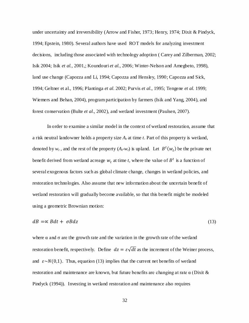
using a geometric Brownian motion:

(13)

where α and σ are the growth rate and the variation in the growth rate of the wetland

restoration benefit, respectively. Define as the increment of the Weiner process,

and . Thus, equation (13) implies that the current net benefits of wetland

restoration and maintenance are known, but future benefits are changing at rate α (Dixit &

Pindyck (1994)). Investing in wetland restoration and maintenance also requires

33

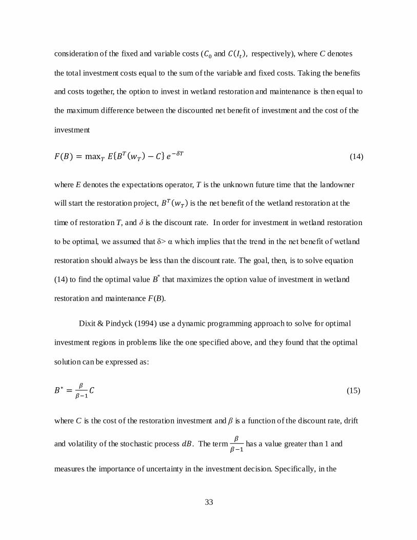
consideration of the fixed and variable costs ( and respectively), where C denotes

the total investment costs equal to the sum of the variable and fixed costs. Taking the benefits

and costs together, the option to invest in wetland restoration and maintenance is then equal to

the maximum difference between the discounted net benefit of investment and the cost of the

investment

(14)

where E denotes the expectations operator, T is the unknown future time that the landowner

will start the restoration project, is the net benefit of the wetland restoration at the

time of restoration T, and δ is the discount rate. In order for investment in wetland restoration

to be optimal, we assumed that δ> α which implies that the trend in the net benefit of wetland

restoration should always be less than the discount rate. The goal, then, is to solve equation

(14) to find the optimal value B* that maximizes the option value of investment in wetland

restoration and maintenance F(B).

Dixit & Pindyck (1994) use a dynamic programming approach to solve for optimal

investment regions in problems like the one specified above, and they found that the optimal

solution can be expressed as:

(15)

where C is the cost of the restoration investment and β is a function of the discount rate, drift

and volatility of the stochastic process . The term

has a value greater than 1 and

measures the importance of uncertainty in the investment decision. Specifically, in the

34

presence of uncertainty, one would invest in wetland restoration and maintenance when the

net benefits of the investment exceed the investment cost by a hurdle rate equal to the option

value of investment. Dixit & Pindyck (1994) go on to show that the critical value of the

investment B* is increasing in the volatility of the growth rate (σ) and trend (α) of net benefit

Although this modeling approach is appealing, it is difficult to test the model‟s

implications because of the intense data requirements. Thus, the majority of studies regarding

land use under uncertainty and irreversibility tended to rely on simulation frameworks, where

Mont-Carlo or other simulation methods are used to test the implication of the ROT model.

3.3. Implications for a Potential Wetland Restoration Policy

Caffey et al. (2003) listed several policy instruments that can be used to encourage

private wetland restoration in the coastal zone, including cost-sharing subsidies, tax reduction,

wetland mitigating banking, and carbon credits. As an example of how these can be

incorporated into the theoretical model, consider the effects of cost-sharing subsidies such as

the one offered under Wetland Reserve Program (WRP) or Conservation Reserve Program

(CRP). Under the WRP, landowners can enter a contract agreement with the government to

reach certain restoration goals, and in exchange they receive rental payments over the contract

period. The program also pays a portion of the total restoration costs. It is worth mentioning

that subsidy programs such as WRP and CRP were largely designed to address the issue of

wetland restoration for land that was devoted to agricultural uses, but modified versions of

these programs can potentially be used to address the issue of wetland restoration in the

coastal zone (Ryan and Susman, 2003).

35

Suppose that a coastal landowner participates in a cost sharing program similar to one

under the WRP, where the landowner will receive a dollar rental payment equal to s per acre

over the contract period k, and the program will pay a portion γ of the total restoration costs.

The landowner‟s decision problem, including the new benefits of the subsidy program, can be

expressed as follows:

(16)

subject to

The landowner‟s maximization problem for each time period can be expressed as:

(17)

subject to

Notice that the cost-share subsidy program adds two terms to the maximization problem – the

cost share portion that the pays and the rental payment over the contract

period k, .

Setting the Hamiltonian function to solve the optimization problem in equation 17 yields:

(18)

36

The first-order conditions for maximization can then be expressed as:

(18.1)

(18.2)

(18.3)

(18.4)

Combining equations (18.1) and (18.2) yields

(19)

Then, using the property of the expected value of the product of two random variables,

(20)

or

(21)

37

Simplifying yields

(22)

The term on the LHS of the equation above is the expected marginal benefits associated

with restoration level . The first term on the RHS is the expected marginal cost associated

with restoring acres of wetland, while the second term is the expected marginal negative

benefit associated with αt wetland loss. The third term on the RHS is the increase in the

marginal benefit of wetland restoration due to cost-share subsidy programs. The last term on

the RHS is non-zero to the extent that it measures the deviation of the risk-averse landowner

from a risk-neutral landowner. It represents the additional cost of risk and it is negative for a

risk averse landowner, and positive for a risk taker landowner. From equation (22), the

subsidy payment and the cost share payment

lower the

hurdle rate for investment in wetland restoration and maintenance. Therefore, the subsidy

program should encourage private landowners to undertake wetland restoration and

maintenance.

This chapter presented the conditions under which the landowners would invest in

wetland restoration and maintenance, finding that uncertainty and fixed costs can play

important role in the decision making process. In a static setting, risk-aversion influences the

trigger value of the decision to invest in wetland restoration projects. However, in a dynamic

setting, the option value of investment under uncertainty influences the decision making

38

process of the landowners. The remainder of the dissertation develops these ideas in an

empirical context with the goal of testing the theoretical implications of this model structure.

39

CHAPTER 4

EMPIRICAL ANALYSIS

The theoretical framework for the landowners‟ decisions to invest in wetland

restoration and maintenance in the presence of risk and uncertainty was developed in both

static and dynamic contexts. The static framework emphasized the role of risk aversion in the

decision process, while the dynamic framework emphasized the role of option value in the

decision process. This chapter develops an empirical model for the factors that influence

decisions to invest in wetland restoration and maintenance. Given that the data for the study

came from a cross sectional survey, the empirical model focuses on analyzing the factors that

influence the landowner‟s decision to invest in wetland restoration and maintenance in the

presence of risk and uncertainty at the time the survey was taken. Hence, the model developed

here is grounded in the static framework approach and emphasizes the important role of risk

aversion and fixed costs in the landowners‟ decision process.

The majority of studies that have looked at factors influencing private investments in

resource stocks similar to wetlands have either used discrete choice models with probit or

logit estimators (Romm et al., 1987; Soule et al., 2000; Koundouri et al., 2006) or a corner

solution model employing a Tobit model (Norris and Batie, 1987; Featherstone and Goodwin,

1993; Hagos and Holden, 2006). The first modeling approach provides useful information on

how different characteristics of the landowners and their wetland tracts influence the

probability of investment in wetland restoration and maintenance, but it does not provide

information on the impact of these factors on the level of investment in wetland restoration

and maintenance. Since the objective of this study was to provide information on the level-of-

investment decision, using a discrete choice model is not optimal. The Tobit model, on the

40

other hand, is particularly useful for analyzing the impacts of landowners‟ characteristic and

their properties on the probability and the level of investment in wetland res toration and

maintenance. In addition, the marginal effects calculated from the estimated Tobit model can

be used to predict the effects of changing the levels of explanatory variables on both the

amount of investment and the probability of investment. The Tobit model, however, is very

restrictive in its parameterization. First, it assumes that the same stochastic process influences

the probability of investment and the level of investment. Second, all zero observations of the

dependent variable are attributed to corner solutions (Blundell and Meghir, 1987; Moffatt,

2005). Because of these limitations, we explore an alternative approach to modeling the data

structure – the double-hurdle model. The double-hurdle model generalizes the Tobit model by

introducing an additional hurdle which must be passed before observing any positive

investments. The additional hurdle uses a probit estimator to model the decision to

invest(discrete variable); therefore, zero observations on the dependent variable can be either

attributed to corner solutions or nonparticipation in the market ( i.e., landowners have never

invested in wetland restoration projects). In doing so, the double hurdle model also allows the

decision to invest in wetland restoration and the level of investments to be treated separately.

Therefore, a separate stochastic process can be used to model the probability of investment

and the level of investment (Carroll et al., 2005).

After briefly introducing the underlying theory of the Tobit model and its limitations,

the discussion in this chapter turns to the double hurdle model as an alternative to the Tobit.

Also presented is a brief section on how the marginal effects are computed and the associated

standard errors for statistical inferences. To close, the last section of the chapter discusses the

issues of heteroskedasticity and non-normality of the error terms in the double hurdle model.

41

4.1 The Tobit Model

Estimating an econometric model of landowner decisions to invest in wetland

restoration and maintenance is complicated by the relatively large number of zero

observations that are usually observed in the dependent variable (i.e., level of private

investment in wetland restoration and maintenance). When the dependent variable is limited

in such a way, analyzing the data using ordinary least square (OLS) may result in biased and

inconsistent estimated parameter (Amemiya, 1984). Discarding zero observations of the

dependent variable is not a viable solution, as doing so and using OLS only with positive

values of the dependent variable increases the potential bias and inefficiency while ignoring

potentially valuable information embedded in the zero observation responses. (Amemiya,

1984). To address these limitations, Tobin (1958) crafted an approach that came to be known

as the Tobit model. To account for the censored nature of data, the Tobit model expresses the

observed response variable y in terms of an underlying latent variable:

if

(23)

if

(24)

where is a latent variable describing the level of investment for landowner , is the

actual level of investment for a landowner , xi is a vector of potential explanatory variables

that influence the landowner‟s decisions to invest in wetland restoration and maintenance, β is

a vector of the associated parameters, and is the error term. The density of given x i is

the same as the density of given x i for positive observations, so the probability that

equals 0 can be expressed as

42

(25)

where (.) is the standard normal cumulative distribution.

The most common approach to estimating the Tobit model is the maximum likelihood

estimator. First, the observations are divided into two groups; censored observations (zero

values of the dependent variable) and the observed positive values of the dependent variable.

The log likelihood function for the Tobit model is expressed as follows:

(26)

where (.) and φ(.) are the standard normal cumulative distribution and the standard normal

density functions, “0” indicates summation over zero observations, and “+” indicates the

summation over positive observations(Greene, 2003).

The parameter estimates of the Tobit model provide little value besides indicating the

significance of the explanatory variable and, if significant, the direction (positive or negative)

of its influence on the dependent variable. Thus, marginal effects are calculated from the

estimated model to more fully understand the magnitude of the relationship between the

explanatory and dependent variables. Using the McDonald and Moffitt (1980) decomposition,

the unconditional expected value of the double hurdle model was expressed by Wooldridge

(2002) as

(27)

From equation (23), the probability of observing a positive investment level for landowner is

(28)

while the conditional expected value of given that is

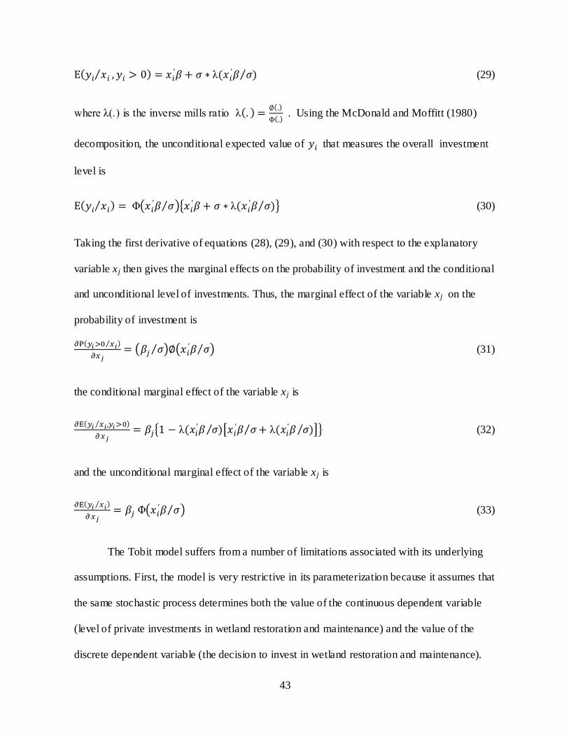
43

(29)

where (.) is the inverse mills ratio

. Using the McDonald and Moffitt (1980)

decomposition, the unconditional expected value of that measures the overall investment

level is

(30)

Taking the first derivative of equations (28), (29), and (30) with respect to the explanatory

variable xj then gives the marginal effects on the probability of investment and the conditional

and unconditional level of investments. Thus, the marginal effect of the variable xj on the

probability of investment is

(31)

the conditional marginal effect of the variable xj is

(32)

and the unconditional marginal effect of the variable x j is

(33)

The Tobit model suffers from a number of limitations associated with its underlying

assumptions. First, the model is very restrictive in its parameterization because it assumes that

the same stochastic process determines both the value of the continuous dependent variable

(level of private investments in wetland restoration and maintenance) and the value of the

discrete dependent variable (the decision to invest in wetland restoration and maintenance).

44

This assumption is very restrictive because the factors that affect a landowner‟s decision to

invest in wetland restoration and maintenance (i.e., the characteristics of the landowners and

their properties) might differ significantly from the factors that influence a landowner‟s

decision about how much to invest in wetland restoration and maintenance. Furthermore, the

same stochastic process assumption implies that if a particular variable is known to have a

positive effect on investment level, then a high value for this variable will inevitably lead to

the prediction of a high probability of investment (Blundell and Meghir, 1987; Moffatt, 2005).

Second, the Tobit model assumes that all zero observations are standard corner solutions or

negative values of the underlying latent variable (Blundell and Meghir, 1987). In the context

of our study, it is possible to imagine cases where the landowners do not invest in wetland

restoration and maintenance for reasons beyond simple economic factors such as income and

relative prices. For example, landowners might decide not to invest in wetland restoration

and maintenance because they don‟t believe a wetland restoration technology exists to do the

task or because they do not believe that they are responsible for restoration, especially

considering that the majority of wetland benefits are public in nature (Heimlich et al. 1998). It

is also possible that landowners may perceive wetland investment to be beneficial (i.e.,

positive value of the latent variable), but for other unmeasured reasons choose not to invest,

thus yielding zero values for the dependent variable.

Unlike the Tobit model, the double-hurdle model allows the decision to invest in

wetland restoration and the level of investments to be treated separately. Therefore, a separate

stochastic process can be used to model the probability of investment and the level of

investments. The next section presents the general function of the double hurdle model and

discusses its underlying assumptions.

45

4.2 Double Hurdle Model

The double hurdle model proposed by Cragg (1971) generalizes the Tobit model by

introducing an additional hurdle which must be passed before observing any positive

investments. Conceptually, a landowner first decides whether or not to invest in wetland

restoration and maintenance. Then, if the decision is made to invest, the landowner decides

how much to invest. A different latent variable is used to model each decision process, with a

probit estimator used to model the participation decision and a Tobit estimator used to model

the level of investment decision (Blundell and Meghir, 1987).2 Therefore, the double hurdle

model allows for the possibility that factors affecting the decision to invest in wetland

restoration and maintenance might differ from factors that affect the level of investment

decision. For example, fixed costs may affect the decisions to invest in wetland restoration

and maintenance, but they may not affect the decisions about how much to invest. In addition,

the double-hurdle model allows the same explanatory variable to have different impacts on

the decisions to invest and the level of investment.

Unlike the Tobit model, which assumes that all zero observation on the dependent

variable are attributed to corner solutions, the double hurdle model allows zero observations

on the dependent variables to be caused by either a simple corner solution (negative value for

the underlying latent dependent variable) or non-participation in the market (i.e., landowner

decides not to invest in wetland restoration projects for some non-modeled reasons) (Moffatt,

2005; Carroll et al., 2005). The general equations of the double-hurdle model can expressed

as follows: 2 The double hurdle model uses a probit model, and not a logit model, in the first stage because the normality

assumption of the error term matches the underlying assumption for the Tobit model. Since both the decision to

invest and how much to invest are based on the same underlying utility function, then the error terms in both

model should follow the same d istributional assumptions.

46

: first hurdle equation (investment decision) (34)

: second hurdle equation (investment level decision) (35)

if

and (36)

otherwise (37)

,

where is a latent variable representing the decision to invest in wetland restoration and

maintenance for a landowner , is a latent variable representing the level of investment for

a landowner , is the observed level of investment for a landowner , zi is a vector of

potential explanatory variables that influence the landowner‟s decision to invest in wetland

restoration and maintenance, xi is a vector of explanatory variables that affect the

landowner‟s level of investment, and α and β are vectors of parameter. In this formulation, (zi

; xi ) may contain the same common explanatory variables, although their corresponding

effects on the two hurdle equations might be quite different. The terms are normal

and independently distributed error terms such that (Carroll et al., 2005).

As might be apparent from this discussion, the Tobit model is just a special case of the

double-hurdle model, where zi = x i and α = β/σ. As a result, the model specification of the

double-hurdle model can be tested against the Tobit model using a likelihood ratio test (LR).

The LR test compares the log- likelihood values of the two models and determines if they are

significantly different from each other (Wooldridge, 2002). The result of this test can be used

to determine whether the landowners make investment decisions in a sequential or

simultaneous manner. If the LR test rejects the null hypothesis of a univariate Tobit, then the

double-hurdle model is preferred and landowners are found to make investment decisions in a

47

sequential two-step process. If, however, the null hypothesis is not rejected, then landowners

are found to make investment decision in a simultaneous manner and the univariate Tobit is a

better representation of the data.

As in the Tobit model case, the most common method for estimating the double-

hurdle model is the maximum likelihood estimator, and its general log- likelihood function can

be expressed as follows (Cragg, 1971):

(38)

where “0” indicates summation over zero observations, “+” indicates the summation over

positive observations, and (.) and φ(.) are the standard normal cumulative distribution and

the standard normal density function, respectively.

Similar to the Tobit model, the parameter estimates of the double hurdle model

provide little direct information beyond the significance and direction of influence for each

explanatory variable, resulting in the need for marginal effect calculations. Using the

McDonald and Moffitt (1980) decomposition, the unconditional expected value of the double

hurdle model can be expressed as (Jensen and Yen, 1996)

(39)

where is the probability of investment and is the conditional

expected value of investment (i.e., the level of investment conditional on having made the

choice to invest). Following Burke‟s (2009) notation, the probability of investment is

48

(40)

.From the Tobit model in the second-hurdle, the conditional expected value of y given that

y>0 is

(41)

where λ(.) is the inverse Mills ratio. After substituting equations (40) and (41) into equation

(39), the unconditional expected value of y can be expressed as follows

(42)

Taking the first derivative of equations (40), (41), and (42) with respect to the explanatory

variable xj yields the double-hurdle marginal effects of the explanatory variable xj on the

probability of investment and the conditional and unconditional level of investments. So, the

marginal effect of the explanatory variable xj on the probability of investment is expressed as

(43)

and the conditional marginal effect of the explanatory variable xj given that landowners have

made a positive investment is

(44)

and the unconditional marginal effect of the explanatory variable xj is

(45)

49

Although having the calculated marginal effects is useful, for statistical inference there

is a need for the standard errors of the estimated marginal effects. These standard errors can

be approximated using the delta method. Denoting the parameter estimates of the double

hurdle model by the vector and the estimated marginal effect for a given

continuous variable in the model by the function , the estimated variance of the

marginal effect using the delta method can be expressed as (Wooldridge, 2002):

(46)

where is the asymptotic variance of the maximum likelihood estimator for and the

standard errors can be computed using the square root of the equation above. This procedure

is employed by the „nlcom’ subroutine in STATA to calculate the standard errors for the

estimated marginal effects of the double hurdle model.

4.3 Heteroskedasticity and Non-normality

The maximum likelihood estimates of the double hurdle model are derived under the

assumption that the error terms and are homoskedastic. In the case of cross-sectional

data, this homoskedasticity assumption is likely to be violated, leading to a situation where

the maximum likelihood estimation produces inconsistent parameter estimates (Arabmazer

and Schmidt, 1981; Maddala, 1975; Hurd, 1979). Arabmazer and Schmidt (1981) investigated

the impact of heteroskedasticity in the Tobit model and found that the size of inconsistency3

increases with heteroskedasticity and the degree of censoring. Hurd (1979) found that

3 Consistency is a very important characteristic of any estimator. It reflects the behavior of the sampling

distribution of the estimator as the sample size increases. An estimator is said to be consistent if it converges to

the parameter estimates of the true population value of the parameter as the sample size increases indefinitely

(Wooldridge,2002)

50

moderate heteroskedasticity in the errors will cause substantial inconsistency in the parameter

estimates. One way to overcome the inconsistency is by assuming that the standard deviation

of the error term is a function of a set of exogenous variables

(47)

where might contain all continuous variables in or just a subset of the continuous

variables suspected for heteroskedasticity and δ is a conformable parameter vector (Su and

Yen, 1996; Jenson and Yen, 1996). A likelihood ratio test (LR) can be used to test the

restrictions (Ho: =0) against the alternative that is not 0. A rejection of this test indicates

that the errors are heteroskedastic.

Similar to the case of heteroskedasticity, the maximum likelihood estimates of the

double hurdle model are very sensitive to the normality assumptions concerning the error

terms and . If normality is violated, the maximum likelihood approach produces

inconsistent parameter estimates (Arabmazer and Schmidt, 1982). One way of dealing with

the non-normality issue is to use a logarithmic transformation of the dependent variable, but

this option is not appropriate in the presence of a large number of zero observations. Another

way to account for non-normal errors is to use a Box-Cox transformation of the dependent

variable, often expressed as (Jenson and Yen, 1996)

(48)

Notice that the logarithmic and the linear transformations are special cases of the Box-Cox

transformation when =0 , and =1, respectively. In general, however, would be expected

51

to take on a value between zero and one (Moffatt, 2005). The log likelihood function of the

double hurdle model after applying the Box-Cox transformation can be expressed as

(49)

This chapter presented two potential models (Tobit and the double hurdle) that can be

used to investigate landowners‟ decisions concerning investment in wetland restoration

projects. The next chapter examines the process used to collect the data needed to statistically

estimate these models and gives an over-review of the data itself.

52

CHAPTER 5

SURVEY DESIGN AND DATA SUMMARY

Chapter 4 presented an empirical framework for modeling the landowner decision

making process with respect to wetland restoration and maintenance. From the theoretical

framework discussed in Chapter 3, risk aversion becomes a key determinant of the

landowners‟ investment decisions. In order to test this theoretical hypothesis, however, a

measure of the risk preferences for private landowners is required. A survey of coastal

landowners in Louisiana was conducted in the fall of 2009 in order to elicit these risk

preferences. Three different risk preference elicitation methods were used in the survey: 1) a

self ranking question on risk preference; 2) a multi- item scale approach; and 3) the expected

utility framework through hypothetical investments distributions with different levels of risk

and expected net returns. The survey was also used to collect other information regarding

landowners‟ investment decisions, their socioeconomic characteristics, and the characteristics

of landholdings. This chapter describes the survey process and presents a descriptive analysis

of the response. The chapter begins with an examination of the survey design and discusses

the general response characteristics. Next, the risk preference elicitation methods that were

used are described. Finally, a summary of the survey data is presented.

5.1 Survey Design and Response

The survey questionnaire (see Appendix A) was designed using Dillman‟s (1978) total

design method for mail surveys. A mailing list of private wetland landowners in coastal

Louisiana was obtained from the Louisiana Department of Natural Resources (LADNR)

geographic information system (GIS) database. This database covers all coastal wetland

landowners who may have potentially been affected by wetlands loss and/or publically funded

53

wetlands restoration and maintenance activities. In it raw form, the GIS database provided by

LADNR had 721 landowners with wetland properties in the coastal zone. However, after

eliminating duplicate names, names without mailing addresses, and publicly owned properties

(such as state-owned wildlife refuges), the mailing list contained a total of 591 landowners.

Using the 591 landowners as the sample frame, we stratified landowners into three

groups based on the number of wetland tracts they owned. The first group included all

landowners with only one tract of land. The second group included all landowners with two

tracts, and the third group included all landowners with more than two tracts (with this latter

group mainly consisting of large corporations). This stratification of the sample based on the

number of tracts was used for several reasons. First, the survey questionnaire asked questions

that are specific to a tract of land, such as the level of investment that was made, income

derived from the land, land use, and the level of wetland loss. Because a landowner with

multiple land tracts might make different investment decisions for each tract, it was important

to have the landowner focus on a specific tract when answering the questionnaire. Second,

stratification (and more specifically, having the responses tied to a specific tract of land)

allowed the response data to be merged with the LADNR GIS information for a land tract

(i.e., location of the land tract, distance from the shoreline, wetland loss, wetland area, and

wetland type).

For this study, the survey questionnaires were mailed to landowners with one or two

tracts of land (groups one and two). As mentioned early, the third group of landowners

consists mainly of large corporations, and they were excluded from this study in part due to

the difficulty in conceptualizing a way to elicit risk preferences from an entity other than an

individual. The behavior of these large landholders is certainly of interest when considering

54

coastal wetland restoration and maintenance, and future research will need to focus on this

problem.

In early fall of 2009, a pre-test version of the survey questionnaire was mailed to a

random sample of 30 private landowners who owned one tract of land (group 1). Based on the

result of this pre-test, changes were made to the survey questionnaires and a final version was

mailed out to all landowners in the sample frame who owned one or two tracts of land (groups

1 and 2). In total, the survey was mailed to a sample size of 378 private landowners. 4 Each

survey questionnaire included an aerial photography map of the landowner‟s property with

location data identified (see figure 5.1 for an example of one of these maps). For landowners

with two tracts of land, they were given two separate maps (one for each tract) and asked to

select the tract of land that they were going to use when answering the survey questionnaire.

As a result, all survey questions that were land-specific referred to well- identified tracts, and

thus could be related (both for this study and in the future) to biophysical features tracked by

other scientific studies.

The survey questionnaire consisted of five sections with a total of 37 questions. The first

section of the survey included a range of questions concerning the participation of the

landowners in government programs, their attitudes toward wetland restoration, and their

attitudes toward various incentive instruments for wetland restoration. More specifically,

landowners were asked about their general attitudes toward wetland restoration, whether they

were aware of any wetland restoration programs in their areas, and if so, whether they had

4 The entire survey process involved the following steps. A pre-notification postcard was sent to all private

landowners, followed by a first mailing of the questionnaire; thank you reminder postcards were mailed out to

landowners shortly thereafter. Approximately two weeks later, a second mailing of the questionnaire was sent

out to all first mailing non-respondents, and shortly after that they were sent a second thank you reminder

postcard. Finally, a third mailing of the questionnaire was sent out to all landowners who did not respond in the

first two attempts. In all, six attempts were made to reach the landowners for a response.

55

enrolled in any of these programs. They were also asked whether they would be willing to

participate in any government-sponsored restoration program and their attitudes toward

various incentive instruments such as tax breaks, subsidies, and cost sharing were elicited.

The second section of the survey was designed to collect information on the general

characteristics of landholdings, such as property size, percentage of wetland, current land use,

ownership type, when the property was first acquired, how it was managed, how much

wetland had been lost, the percentage of household income generated from both surface and

sub-surface activities, and the expected market value of the property. The third section of the

survey asked questions regarding investment in wetland restoration and maintenance. In this

section, landowners were asked whether they had conducted any wetland restoration and

maintenance activities, the year in which they started these restoration projects, the type of

restoration techniques they had used, the level of private investment expenditures they had

made on wetland restoration and maintenance activities, and the level of public investment

expenditures that had been made on wetland restoration and maintenance activities. In this

section of the survey, the landowners were also asked about the factors that motivated or

deterred them from conducting wetland restoration and maintenance activities, their

perceptions about the source and level of uncertainty faced in wetland restoration and

maintenance activities, and their general attitudes toward wetland restoration and

maintenance. The fourth section included demographic questions, such as education, income,

age, gender, and place of residence. The final section of the survey elicited the landowners‟

risk preferences. Three risk preference elicitation methods were used: self ranking, multi- item

scale, and the direct expected utility method using hypothetical investment distributions with

different levels of returns and risk.

56

Figure 5.1: An example of an aerial photography map of a wetland tract in Louisiana’s

coastal zone. In the survey questionnaire, the boundary of the tract was clearly marked

and geospatial information about the location of the tract was also provided to help

respondents identify the wetland tract.

57

Of the original 378 survey questionnaires that were mailed out, 48 were not deliverable

and 75 were returned completed. Removing the undelivered questionnaires from the sample,

the survey response rate was approximately 23%. The respondents owned a total of 393,680

acres, or approximately 57% of the total acreage owned by all 378 landowners in the sample

frame. In term of the total wetland acreage controlled by the survey respondents, we found

that survey respondents controlled approximately 6% of the total wetland acreage in

Louisiana‟s coastal zone (3.4 million acres). If one takes out the total wetland acreage owned

by the top 50 corporations and the lands owned by the state such national refuges and wildlife

management areas 5 in the sample frame, we found that the survey respondents controlled

about 11% of the total wetland acreage in the coastal zone of Louisiana based on a very

conservative assumption about the wetland percentage on these properties. Figure 5.2 presents

the distribution of the survey respondents across the coastal zone of Louisiana.

5.2 Risk Preference Elicitation Methods

Three risk preference elicitation instruments were employed to measure the risk

preferences of landowners: a self ranking question on risk preference, a multi- item scale

approach, and the expected utility framework through hypothetical investments distributions

with different levels of risk and expected net returns.

5.2.1 The Self Ranking Risk Method

Landowners were asked to rank their personal preferences for taking investment risks

using a 10-point scale, with 1 being risk-hating and 10 being risk- loving. Previous studies

5 The top 50 landowners in our sample frame controlled approximately 2.7 million acres of land, but it is

unknown how much wetlands they controlled. Our survey data showed that, on average, landowners reported

that 76% of their propert ies are wet lands( see table 5.3). We used a more conservative estimate to estimate the

total wetland acreage controlled by the top 50 corporat ions. We used 50% rate as a base. Hence, it is estimated

that the top 50 corporations controlled about 1.35 million acres of wetlands. The wild life management areas in

the sample frame controlled about 554,215 acres of land in coastal zone of Louisiana .

58

have employed the self ranking risk method (Cardona, 1999; Henderson, 2007; Thomas,

1987; Schurle and Tierney, 1990; Faust and Gillespie, 2006) and compared the self ranking

risk method to other risk elicitation methods, including interval and “closing- in” approaches

(Thomas, 1987; Schuler and Tierney, 1990; Bard and Barry, 2001; Faust and Gillespie, 2006).

The results of these studies are mixed, with some finding a significant correlation between

the self-ranking risk preference elicitation method and other methods (Schuler and Tierney,

1990; Thomas, 1987; Fausti and Gillespie, 2006) and others find no significant relationship

between the self- ranking method and other methods (Bard and Barry, 2001).

Figure 5.2: Distribution of the survey respondents across Louisiana’s Coastal zone.

5.2.2 Multi-item Scale Approach

In the psychological literature, the term “attitudes” refers to clusters of feelings,

beliefs, and behavioral tendencies that are not directly observable (Baron and Byrne, 1981).

Therefore, risk attitudes are latent variables that can be measured indirectly through a set of

59

indicator variables that are correlated with these latent variables. To measure risk attitudes

using a multi- item scale approach, individuals are given a set of questions or items and asked

to indicate the degree to which they agree or disagree with each question. This approach was

found to perform well in terms of reliability and validity, and it is commonly used to measure

the risk preferences of individuals (Penning and Garcia, 2001). For this study, landowners

were asked to indicate on scale from 1 (” I strongly disagree”) to 5 (“ I strongly agree”) the

extent to which they agreed with a set of statements (Table 5.1) that were selected to „tap‟ the

domain of the construct as recommended by Churchill (1995). Example applications of the

scale approach can be found in the economic literature. Goodwin and Schroeder (1994)

measured the risk attitudes of farmers using a binary variable of whether the farmers had

preferences for business risk. Penning and Garcia (2001) measured the risk preferences of hog

farmers using the multi-scale approach, where the farmers were give seven statements and

asked to indicate the degree to which they agreed with each statement. The study found that

the risk attitudes measured using the multi- item scale approach were statistically related to

risk attitudes measured using the expected utility framework.

5.2.3 Investment Method

The investment method of risk elicitation used in this study closely followed the

experimental design developed by Gunjal and Legault (1996) and used the certainty

equivalence concept associated with the expected utility model. Table 5.2 presents the basic

structure of the experiment. The landowners were given seven investment distributions with

various levels of net returns and risks. Each investment distribution had three outcomes (low,

average, and high) with equal probability of any of the outcomes occurring. The landowners

were asked to select one of the investment distributions as being the most preferred, where the

60

distributions were calculated using the Constant Partial Risk Aversion (CPRA) utility function

of the form: where is the certainty equivalent of the risky prospect

and is the coefficient of risk aversion. The outcomes of the investment distributions were

calculated such that two adjacent investment distributions had the same expected utility value.

In addition, the investment distributions were generated under the implicit assumption that the

majority of landowners are risk averse. Landowners who selected investment options 1 to 4 in

Table 5.2 were classified as risk averse. Landowners who selected investment option 5 in

Table 5.2 were classified as risk neutral, while landowners who selected investment options 6

and 7 were classified as risk-takers. The upper and the lower limits of the coefficients of the

constant partial risk aversion for each distribution are reported in Table 5.2. To investigate the

changes in partial risk aversion for each landowner, we increased the level of investment by

factors of 4 and 10.

Table 5.1: Statements used to elicit the landowners’ risk preference

1. I like taking financial risks

2. I try to avoid investment risks

3. I am willing to take financial risks in order to realize higher returns

4. I prefer to receive a guaranteed return even if it is low

5. It is unlikely that I would invest in a business if it has a chance of failing

6. When making investment decisions I attach equal weight to maximizing long-term returns and minimizing financial risks.

7. I aim to achieve high long-term returns on my investments even if

that means taking significant financial risks in the short-run

8. I prefer to receive a guaranteed low return on my investments

rather than an uncertain high return

61

Table 5.2: An example of the basic structure of the investment method experiment using

a $25,000 investment level

Investment

option

Lowest

net

return

Average

net return

Highest

net return

Partial risk aversion

interval

1 $2,500 $2,500 $2,500 +infinity to 7.47

2 $2,271 $2,600 $2,930 7.47 to 2

3 $1,989 $2,700 $3,412 2 to 0.85

4 $1,603 $2,800 $3,997 0.85 to 0.32

5 $962 $2,900 $4,838 0.32 to -0.32

6 $372 $2,800 $5,228 -0.32 to -0.45

7 $0 $2,700 $5,400 0.45 to -infinity

5.3 Descriptive Summary of Survey Results

5.3.1 Demographics

Table 5.3 presents a summary of the demographic variables collected from the

respondents. The vast majority of the respondents were male (93.15%) and Louisiana

residents (92%). The average age for the respondents was just under 62 years, with a range of

22 to 90 years old. The vast majority of the respondents were college graduates (57.53%),

with 15.07% of the respondents having some college education and the remaining 27.4% of

the respondents having no college education.

62

Table 5.3: Demographic characteristics of the respondents

Variable Percent (%) Cumulative percent (%)

Education attainment

Some high school (or less) 4.11 4.11

Completed high school or GED 15.07 19.18 Trade or technical school graduate 8.22 27.4

Some college 15.07 42.47 College graduate 57.53 100

Gender

Female 6.85 6.85 Male 93.15 100

Household total income

Under $15,000 1.67 1.67

$15,001 to $30,000 8.33 10 $30,001 to $50,000 6.67 16.67

$50,001 to $70,000 6.67 23.33 $70,001 to $100,000 11.67 35

$100,001 to $150,000 23.33 58.33 $150,001 to $200,000 16.67 75

Over $200,000 25 100

Residency

No Louisiana residence 8.22 8.22

Louisiana residence 91.78 100

Home location

Does not live on the property 90.41 90.41 Lives on the property 9.59 100

The income question was the most frequently skipped demographic question, with

only 60 out of the 75 respondents providing information about income level. As reported in

Table 5.3, 35% of the respondents had incomes of $100,000 or less, and 23% of the

respondents had incomes in the range of $100,001 to $150,000. In additions, 17% of

63

respondents had incomes in the range of $150,001 to $200,000, and 25% of the respondents

reported annual incomes over $200,000, The majority of the landowners (90.41%) reported

that they did not live on the properties that were identified in the questionnaire.

5.3.2 Attitudes Toward Wetland Conservation and Various Incentive Programs

Landowners were asked to indicate the extent to which they agreed or disagreed with

various statements relating to wetland restoration. First, the landowners were asked, a general

question about the importance of wetland restoration to future generations. The majority of

the respondents (91%) either strongly agreed or agreed with this statement. Then the

landowners were asked more direct questions about the values of wetland restoration. In

response to the statement, “Restored wetlands protect wildlife and/or fish habitat,” 93% of the

respondents strongly agreed or agreed with this statement. Similarly, about 92% of the

respondents strongly agreed or agreed with the statement, “Restoring wetlands improves

water quality and reduces erosion.” Approximately 90% of the respondents strongly agreed or

agreed with the statement, “Wetland restoration provides storm and flood protection” (see

figure 5.3).

Asked about their awareness of various wetland restoration programs in the coastal

zone, 46% of the landowners indicated that they were aware of wetland restoration programs

in their area. Out of the group of respondents who were aware of wetland restoration

programs in their areas, 47% had enrolled in one or more of the available programs.

Landowners were also asked if they would be willing to participate in future programs, with

the majority of the respondents (86%) indicating that they were willing to participate.

64

Figure 5.3: Respondents’ attitudes concerning the importance of restoring wetlands in

coastal Louisiana

Following this question, the landowners who were interested in participation were asked to

indicate the importance of the following wetland restoration incentive instruments: 1) tax

incentive, 2) cost-sharing assistance, 3) direct grants and subsidies, 4) temporary conservation

easement, 5) permanent conservation easement, 6) wetland mitigation banking, and 7) carbon

credit program. They were asked to rate (on a 5-point Likert scale) the importance of each of

the incentive instruments (see Figure 5.4). The most preferred instrument was direct grants

and subsidies (83% of the respondents rated this option as either somewhat important or very

important). The second preferred instrument was cost sharing assistance, with 66% of the

respondents rating cost sharing as either somewhat important or very important. Tax

incentives were also popular, with about 59 % of the respondents indicating that this program

was either somewhat important or very important. Somewhat less popular were permanent

conservation easements and wetland mitigation banking, but a majority of the respondents

(52% and 51 %, respectively) rated these two instruments either somewhat important or very

important. Temporary easement and carbon credit instruments received considerably less

0% 20% 40% 60% 80% 100%

Restoring wetlands is important for future generations

Restoring wetlands protects wildlife and fish habitats

Restoring wetlands improves water quality and reduces erosion

Restoring wetlands provides storm and flood protection

We

tlan

ds

valu

es

Strongly Disagree Disagree Neutral Agree Strongly Agree

65

support, with 35-36 % of the landowners indicating that these programs were somewhat to

very important.

Figure 5.4: Landowners’ preferences for various incentive instruments for wetland

restoration and maintenance in coastal Louisiana

5.3.3 Characteristics of the Properties

Landowners were asked a group of questions regarding the general characteristics of

their landholdings, including property size, percentage of wetland, current land use,

ownership type, the time that the property was first acquired, how is it managed, and how

much wetland had been loss, the percentage of household income generated from both surface

and sub-surface activities, and the expected market value of the property. A statistical

summary of the main variables in this section is presented in tables 5.4 and 5.5. The results

show that the properties of the landowners who responded to the survey have diverse

characteristics. The total acres owned by respondents ranged from 19 to 150,000 acres, with

an average of 5,249 acres and standard deviation of 17,892 acres. The average wetland

acreage on these properties was 2,764 acres, with a range of 16 to 25,175 acres. In percentage

0% 20% 40% 60% 80% 100%

Tax incentive

Cost-sharing assistance

Direct grants and subsidies

Temporary conservation easement

Permanent conservation easement

Wetland mitigation banking

Carbon credit program

Not important at all Somewhat unimportant

No opinion Somewhat important

Very important

66

terms, wetlands averaged about 76% of the property acreage of the respondents, ranging from

5% to 100%.

Table 5.4: Statistical summary of the property characteristics for respondents to the

landowner survey.

Variable Mean Std Dev Min Max Total

Property size 5,249 17,892 19 150,000 393,680

Wetland percent 75.73 28.18 5 100

Wetland total acres 2,764 4,789 16.4 25,175 193,450

Leased(0,1) dummy

variable 0.43 0.50 0 1

Acres lost 329 1,176 0 800,7 17,417

Leased acres 1,653 4,047 0 25,000 82,635

Table 5.5: Ownership structure and land management

Variable

Percent

(%)

Cumulative

percent (%)

Ownership type

Sole ownership 32 32

Joint ownership through a tenants- in- common

arrangement 20 52

Joint ownership through a corporation or trust 29.33 81.33

Other ownership 18.67 100

Management type

Self-managed 60.81 60.81

Managed using hired a service or employees 12.16 72.97

Managed by leaseholder 8.11 81.08

67

The most common ownership structure among respondents was sole ownership (about

32 % of the properties). The second most common ownership structure was joint ownership

through a corporation or trust, with 29% of the respondents choosing this category. The third

most common ownership category was joint-ownership through a tenants- in common

arrangement, with about 20% of the wetland properties owned in this way. The remaining

19% of the property were owned through some other, generally unspecified structure.

A majority of the respondents (60.81%) indicated that they self-managed their

landholdings (see Table 5.5). The distribution of other management types included the

following: 19% of the respondents had their properties managed by government personnel,

12% of the properties were managed by a hired service or employees, and 8% of the

properties were not being actively managed.

Landowners were also asked in this section of the questionnaire about wetland loss on

their properties and whether they were renting out part of their properties to other landowners.

Although only 53 landowners (out of 75 respondents) provided estimates for wetland loss on

their properties, these losses averaged 329 acres (standard deviation of 1176 acres), or

approximately 14% of the total wetland acres held by the respondents to this question. When

the landowners were asked if they leased out part of their properties, only 43% of the

respondents indicated that they did, with the average lease size being 1,653 acres (standard

deviation of 4,047 acres for the 50 respondents to this question).

Landowners were asked to rate (on a 5-point scale) the importance of each of the

following land activities on the tract of land specified in their questionnaire: 1) agriculture

production, 2) timber production, 3) fur-trapping, alligator hunting and egg production, 4)

68

waterfowl hunting, 5) fishing, and 6) oil and gas activities. The primary land use was

waterfowl hunting, with 57% of the respondents rating this land use option as either important

or very important. The second land use option was oil and gas activities, with about 53% of

the respondents rating this option as either important or very important. Fur-trapping, alligator

hunting and egg production was also a popular land use option, with 40% of the respondents

rating it as either somewhat important or very important. About 39% of the respondents rated

the fishing land use option as either important or very important. Agricultural activities and

timber production were not common in these coastal zone properties, with only 19% and 9%

of the respondents rating these options as either somewhat important or very important,

respectively. Finally, only 9% of the respondents indicated that they used their landholdings

for other types of activities. Figure 5.5 presents a frequency chart of the land use activities.

Figure 5.5: Values assigned by the landowners to various land uses activities associated

with the current use of the property tract

Landowners were asked about the percentages of their annual incomes derived from

surface and subsurface activities on the specific tract of land noted in the questionnaire. The

0% 10% 20% 30% 40% 50% 60% 70% 80% 90%100%

Agriculture production

Timber production

Fur trapping, alligator hunting, and/or egg collection

Waterfowl hunting

All types of fishing

Oil & gas activities

Not very important Unimportant No opinion Important Very important

69

vast majorities of the respondents derived no income from surface (70%) or subsurface

activities (72%). For those respondents with income from surface and sub-surface activities,

the surface income averaged about 12% of their annual income, ranging from less than 1% to

100%. Similarly, subsurface income averaged about 17% of their annual income, ranging

from less than 1% to 88%.

5.3.4. Wetland Investments

Landowners were asked if they made any investment in wetland restoration and

maintenance on the property specified in the questionnaire, and how much they privately

invested over the last 10 years. Only 35% indicated that they had, with the average total

private expenditure over the 10 years period being $31,522 with an associated standard

deviation of $93,265 (Table 5.6). Following this question, the landowners who had

implemented wetland restoration projects were asked about the type of restoration practices

they used. As reported in Table 5.7, the most commonly used practice was the installation of

water control structures, with approximately 62% of the respondents using this me thod .. The

second most commonly used practice was vegetative plantings (54% of the respondents),

followed closely by sediment, dredge or spoil usage (about 50% of the respondents). Finally,

between 20% and 27% of the respondents reported using fresh water inputs, nutrient/sediment

traps, or some other wetland restoration practices.

The landowners who invested in wetland restoration projects were asked, using a 5-

point Likert scale, to indicate the importance of a set of factors related to their decisions to

invest in wetland restoration and maintenance. The most important factor to the respondents

was the desire to protect or enhance the ecological functions of their property (Figure 5.6).

70

Approximately 96% of the respondents rated this factor as either important or very important

in their investment decision to. The desire to protect or enhance the property market value

was listed as an important or very important reason for investing by 82% of the respondents.

Table 5.6. Statistical summary of the continuous variables in the investment section

Variable Mean Std. Dev Min Max

Investment level $31,521.74 $93,265.21 0 $600,000

Invest(0.1)

dummy 0.35 0.48 0 1

Uncertainty 5.10 3.68 0 10

Risk attitude 4.90 2.46 1 10

Table 5.7. Type of wetland restoration practices that the respondents used

Name of restoration practice

Restoration

practice is

used

Restoration

practice is

not used

Water control structures (gates, weirs, etc.) 61.54% 38.46%

Vegetative plantings (trees or grasses) 53.85% 46.15%

Nutrient/sediment traps (brush fences, terraces, etc.) 20% 80%

Sediment, dredge or spoil usage 50% 50%

Increased fresh water inputs to the property 26.92% 73.08%

Others 24% 76%

The availability of restoration subsidies and the desire to protect or enhance the property‟s

revenue generation ability were listed as important factors by approximately 71% and 75% of

the respondents, respectively.

71

Figure 5.6: Respondents’ perceptions about various factors that influence their

decisions to invest in wetland restoration and maintenance

Similarly, landowners were asked about the factors that have prevented them, or might

prevent them in the future, from investing in wetland restoration (Figure 5.7). Potential

respondents were given a list of factors and asked to indicate the importance to each factor

using a 5-point Likert scale. Topping the list of these deterrent factors was the high cost of

wetland restoration, with 75% of the respondents listing this factor as either important or very

important in their decisions not to invest. The second most important factor was insufficient

government financial incentives, with about 69% of the respondents rat ing this factor as

important or very important. Uncertainty about future benefits and costs of wetland

restoration and the lack of personal financial resources were also important, with about 66%

of the respondents ranking these factors as either important or very important. Fifty two

percent of the respondents listed the lack of personal economic benefits from wetland

restoration as an important or very important impediment to investing. At the bottom of the

0% 20% 40% 60% 80% 100%

Availability of restoration subsidies in the form of monetary payments

Availability of restoration subsidies in the form of technical assistance

Desire to protect or enhance the property market value

Desire to protect or enhance the property’s revenue generating ability

Recent improvements in restoration technology

Desire to protect or enhance the ecological functions


72

list of investment impediments was the lack of need for wetland restoration, with only 22% of

the respondents reporting this factor as an important deterrent to investment.

Figure 5.7. Respondents’ perceptions about various factors that influence their

decisions not to invest in wetland restoration and maintenance

Given the reported importance of uncertainty about future cost and benefits in the

investment decision-making process, the landowners were also asked to identify the sources

of uncertainty they were facing. Potential respondents were given a selected set of uncertainty

sources and were asked to rank them (Figure 5.8). Uncertainty about changing government

policies was ranked the number one source of uncertainty, with 50% of the respondents

indicating it to be the most important source of uncertainty and 19% of them ranking it

second most important source. Another important source of uncertainty, as perceived by the

landowners, was shifting environmental conditions, with 58% of the respondents ranking this

as either the first or second most important source of uncertainty. Uncertainty about

restoration costs and restoration technologies were ranked third and fourth, respectively.

0% 20% 40% 60% 80% 100%

High current cost of restoration

Uncertainty about future costs and benefits of restoration

Insufficient government financial incentives

No need for wetland restoration

Lack of personal financial resources for restorations

Lacks of personal economic benefits from restorations


73

Figure 5.8. Respondents’ perceptions about uncertainty sources

Finally, landowners were asked to assess the level of uncertainty associated with

making a positive return on investment in wetland restoration and maintenance projects using

a 0 to 10 scale, with 0 representing no uncertainty and 10 high uncertainty. On average, the

respondents assessed the level of uncertainty to be right in the middle of the range (Table 5.6),

with the average score being 5.10 (standard deviation equal to 3.68).

5.3.5 Landowner Risk Preferences

In total, 72 landowners responded to the self-ranking risk question. The responses of

the respondents ranged from 1 to 10, with a mean of 4.9 ( Table 5.6). The self ranking risk

question did not allow for classifying respondents into risk averse and risk taker groups

because it did not provide a unique measure of the risk preferences of the respondents (such

as the coefficients of the partial risk aversion in the investment method). However, the

distribution of the respondents scores reported in Figure 5.9 was used to shed light on how

landowners assessed their risk preferences compared to other landowners. For example,

0% 20% 40% 60% 80% 100%

Changing government policies

Availability of effective restoration technology

Changing restoration costs

Shifting environmental conditions

Others

1st preference 2nd preference 3rd preference

4th preference 5th preference

74

Figure 5.9 shows that 43% of the respondents reported that they avoided taking investment

risk compared to a respondent with a score of 5 (the median score). In addition, 38% of the

respondents reported that they were willing to take more investment risk than a respondent

with a score of 5.

Figure 5.9. Landowners’risk attitude scores based on the self ranking question

Principal component analysis6 of the multi- item scale approach revealed three important

factors that explained about 72% of the total variation in the sample (Table 5.8). The first

factor had an eigenvalue of 14.66 and explained about 34.11% of the total variation in the

sample, and the second factor had an eigenvalue of 10.31 and explained 24% of the total

sample variation. The third factor had an eigenvalue of 5.97 and explained about 14% of the

total variation in the sample. Three items (4, 5, and 8) out of the total 8 items reported in

Table 5.1 make up the first factor. Since two of these items are related to the return risk, then

the first factor appeared to measure the landowners‟ attitudes toward risk in returns. The

6 Item# 6 in Table1 was excluded from the principal component analysis due to a small and insignificant loading

coefficient.

0

5

10

15

20

25

1 Risk

Hating

2 3 4 5 Median

6 7 8 10 Risk

Loving

Re

spo

nd

en

ts (

%)

75

Table 5.8. Variance matrix of the principal component analysis

Factor

Eigenvalue

(variance)

Variance

explained (%)

Cumulative

variance

explained(%)

Factor 1 14.66 34.11% 34.11%

Factor 2 10.31 23.99% 58.10%

Factor 3 5.97 13.89% 71.99%

Factor 4 5.25 12.21% 84.21%

Factor 5 3.51 8.18% 92.38%

Factor 6 1.88 4.37% 96.76%

Factor 7 1.39 3.24% 100%

second factor was represented by two items (1 and 3), and both of them are related to

financial risk. Hence, the second factor appeared to be measuring the landowners‟ attitudes

toward the financial risk. Finally, item 2 had significant loadings on the eigenvector of the

third factor. The third factor appeared to measure the importance of investment risk (see table

5.9).

The multi- item risk method did not allow for classifying landowners into risk averse,

risk neutral, or risk taker groups. However, principal component analysis can be used to

calculate the scores of landowners associated with each factor, with these factor scores

subsequently used to assess a respondents level of risk preference. Before running the

analysis, all items presented in Table 5.9 were rescaled to take on values of -4 (”I strongly

disagree”) to 4 (”I strongly agree”), with items with negative scores indicating that

landowners avoided taking risk and items with positive scores indicating that landowners

76

were willing to take risk. Consequently, respondents with positive factor scores would

indicate that they were less willing to take risk than respondents with zero factor scores and

respondents with negative factor scores would indicate that they were willing to take more

risk than respondents with zero factor scores. As reported in Table 5.10, results of the first

factor model showed that 43% of respondents indicated they tend to take less risk than

respondents with zero factor scores. However, about 40% of the respondents indicated that

they were willing to take more risk than respondents with zero factor scores. Results of the

other factor models are presented in Table 5.10.

Table 5.9. Factor loading matrix of the principal component analysis

Item Factor 1 Factor 2 Factor 3

I like taking financial risks 0.285 0.597 0.077

I try to avoid investment risks 0.326 -0.369 0.777

I am willing to take financial risks in order to

realize higher returns 0.212 0.598 0.038

I prefer to receive a guaranteed return even if it is

low 0.535 -0.155 -0.047

It is unlikely that I would invest in a business if it

has a chance of failing 0.482 -0.185 -0.459

I aim to achieve high long-term returns on my

investments even if that means taking significant

financial risks in the short-run 0.232 0.264 0.331

I prefer to receive a guaranteed low return on my

investments rather than an uncertain high return 0.442 -0.148 -0.257

Note: factors‟ loadings that are larger than 0.4 are presented in bold. Only the results of the

first three factors are reported in this table.

77

Finally, the distribution of the respondents‟ answers for the investment method

question associated with a $25,000 investment level7 is reported in Table 5.11. In total, only

52 landowners answered this question. The results showed that the vast majority of the

respondents (73%) were classified as risk averse. About 21 % of the landowners were

classified as risk neutral, and only 6% of the landowners were classified as risk takers.

Table 5.10. Landowners’ risk attitudes based on the multi-item scale approach

Factor Avoid taking risk Risk indifferent Like taking risk

Factor 1 43.28% 16.42% 40.30%

Factor 2 38.81% 23.88% 37.31%

Factor 3 37.31% 29.85% 32.84%

Table 5.11. Landowners’ investment distribution choices associated with a $25,000

investment level

Investment option Percent (%) Cumulative percent (%)

1 17.31% 17.31%

2 9.62% 26.92%

3 17.31% 44.23%

4 28.85% 73.08%

5 21.15% 94.23%

6 3.85% 98.08%

7 1.92% 100%

7 Due to large number of missing observations associated with the question regarding the other two investment

levels ($100,000 and $250,000), the results of the risk investment question for a $25,000 investment level is

discussed.

78

Taken together, the survey data collected in this study indicated that the majority of

landowners were risk averse. About 73% of the respondents were classified as risk averse

based on the investment method. The other risk preference elicitation methods did not allow

for specific categorizations of the landowners into risk averse and risk taker groups, but they

showed that a large number of respondents appeared to avoid taking risk in their investment

decisions. A large proportion of landowners placed importance on wetland conservation, with

more than 90% of the landowners either strongly agreeing or agreeing with statements related

to the importance of wetlands for 1) future generations, 2) wildlife and/or fish habitats, 3)

water quality and erosion control, and 4) storm and flood protections. The survey results also

provided important information regarding attitudes toward incentive programs for wetland

restoration and maintenance. The majority of landowners (86%) indicated that they would be

willing to participate in wetland restoration programs. About 83% of these landowners

selected direct grants and subsidies as their most preferred incentive instrument. Cost sharing

assistance and tax incentives were the second and third most preferable incentive options,

respectively.

The primary land uses for respondents to the survey were waterfowl hunting and oil

and gas activities. Timber and agricultural production were the least important land-use

activities in the sample. The vast majority of landowners (70% or more) derived no income

values from their wetland holdings. With regard to investments in wetland restoration and

maintenance projects, only 35% of the landowners had made any wetland restoration

investments. Costs of wetland restoration, insufficient financial incentives, and uncertainty

about future benefits and costs of wetland restoration projects were considered major

deterrents to investment. With regard to the uncertainty sources, the majority of the

79

landowners listed uncertainty about changing government policies, and shifting

environmental conditions as their chief concerns. The next chapter uses this information, and

more, to estimate the empirical models outlined in Chapter 4.

80

CHAPTER 6

RESULTS OF EMPIRICAL ESTIMATION

Two econometric models to analyze landowner investment decisions were presented

in chapter 4 – the Tobit model and the double hurdle model. The Tobit model assumes that

landowners make the decisions to invest and the level of investment simultaneously, while the

double hurdle model assumes that landowners make these decisions sequentially. To explore

the implications of choosing each of these decision making models, this chapter presents

empirical results from the estimation of the Tobit and the double hurdle models, comparing

the results and testing to see which model best represents the survey data. The material is

presented in the chapter as follows. First, a brief summary of the key variables used in the

analysis is presented, followed by the results of the Tobit model estimation. Next, the results

of the double hurdle model estimation are presented and discussed. Lastly, the two

econometric models are compared for their suitability given the collected data.

6.1 Data Summary

Descriptive statistics of the variables selected for the analysis are reported in Table

6.1. Considering the dependent variables, “invest” is a discrete dummy variable that indicates

if the landowners made any wetland investment on their property and “invest level” describes

the level of private investments that were made over the last 10 years. The descriptive

statistics show that majority of landowners did not invest in wetland restoration and

maintenance with only 35% of the respondents indicating that they had done so. But, for those

who did make private investments, the average total investment over the last 10 years was

$31,522 (standard deviation of $93,265).

81

Table 6.1: Summary statistics for the variables used in the analysis

Variable Description Mean Std. Dev

Invest =1 if investing in wetland restoration, 0 otherwise 0.35 0.48

Invest

level Total investment expenditure on wetland restoration($) 31,522 93,265

Wetac Total wetland acres owned or managed 2,764 4,789

Age Landowner's age, in years 61.94 12.4

Educ Landowner's level of education 4.07 1.28

Landinc Total household income related to the property use ($) 8,922 26,828

Sowner =1 of the landowner is a sole-owner, 0 otherwise 0.32 0.47

Govwetrp

=1 if the landowner is enrolled in government wetland

restoration programs, 0 otherwise 0.22 0.41

Pubinv =1 if public investment is made on the property, 0 otherwise 0.12 0.33

Consatt

An index for the landowners attitudes toward wetland

conservation 4.69 0.7

Riskatt A self reported measure of risk attitude 4.9 2.46

Agruse =1 if part of the property is used for agricultural production, 0 otherwise 0.19 0.39

LAresid =1 if the landowner is Louisiana residence, 0 otherwise 0.92 0.28

Distshore Distance from the shore line(miles) 28.6 17.11

Long Longitude(miles) 144.87 88.98

82

6.1.1 Characteristics of Landholdings

A relevant explanatory variable in the decision to invest in wetland restoration and

maintenance is the property size, represented here by the total wetland acreages owned or

operated. Property size was previously found to have a positive effect on investment in soil

conservation (Norris and Batie, 1987; Soule et al., 2000). It was expected that the larger the

wetland size, the larger the level of investment in wetland restoration projects. This variable

was transformed via natural logarithm to allow for a nonlinear relationship between wetland

investments and wetland property size.

Land income (“landinc”) was defined as the total household income level8 derived

from the activities that took place on the respondent‟s wetland property. This variable was

created by multiplying the percentage of income derived from the both surface and sub-

surface activities with the mid-value of the income range that the respondents reported. A

positive relationship between income and the decision to invest was reported in other studies

(Norris and Batie, 1987; Romm et al., 1987; Zhang and Flick, 2001). It was expected that

landowners with higher incomes from their wetland properties would invest more in wetland

restoration and maintenance projects.

Two property location variables were included in the analysis. The first location

variable was the distance of the property (in miles) from the shoreline (Distshore). The

distance of the property from the shoreline was calculated by overlaying the digitalized

property information with the existing GIS map of coastal Louisiana. The distance of the

8 Out of the total sample (N=75), 60 respondents reported their income earn ings. An auxiliary regression was

used to impute the missing data. Income was specified as a function of wetland acres (in natural logarithm) and

education. The regression R-square was 0.41 and all explanatory variab les were h ighly significant. The predicted

incomes from this auxiliary regression were used for the missing observations. The result of this auxiliary

regression is presented in Appendix B. Due to missing observations of the explanatory variables in the auxiliary

regression model, only 11 out of total 15 income missing observations were generated.

83

property from the shoreline was calculated by drawing a straight line between the property

center and the nearest point on the coastal map, and measuring its length. This variable was

included in the model as a proxy for the vulnerability of the wetland property to erosion and

other exogenous, weather related forces. It also captured the impact of wetland type on the

landowners‟ investment decision. Properties that are located close to the shoreline are

generally dominated by salt marshes, and properties located further from the shoreline are

dominated by fresh marshes. It was expected that landowners with wetland properties further

inland are more likely to invest, and invest more, in wetland restoration projects. The second

location variable was the longitude of the property (Long). This variable was included as a

proxy for wetland losses. Historical wetland loss rates and projected losses are concentrated in

the eastern part of the State, and then mainly in the lower Terrebonne, Barataria basins and

Mississippi basins (Louisiana Department of Natural Resources (LADNR), 1999). As such,

the high rate of wetland loss in the eastern part of the state may make investment infeasible

and increases investment risk. Therefore, landowners with properties located in the eastern

part of the state would be less likely to invest in wetland restoration and maintenance projects.

Alternatively, one might argue that the higher the rate of wetland loss in the eastern part of the

state may encourage landowners to invest in wetland restoration projects in order to prevent

additional wetland losses. Thus, the expected sign of this variable is ambiguous. The Long

variable was measured in miles and it increases as the property location moves from wes t to

east.

The use of the property for agricultural production was also hypothesized to influence

the decision to invest in wetland restoration and maintenance. To capture this effect, a

dummy variable for agriculture land use (Agruse) was included in the analysis. Agruse was

84

assigned a value of 1 if a landowner used part of his/her landholding for agriculture

production and 0 otherwise. It was hypothesized that landowners who use part of their

properties for agricultural activities were less likely to invest in, wetland restoration projects

than other landowners due to diminishing surface and subsurface wetland incomes, time

constraints, and changes in operational focus.

6.1.2 Characteristics of the Landowners

Characteristics of the landowners included both demographic variables and attitudes

toward risk and wetland conservation issues. The demographic variables included age,

education, and residence, and ownership structure. Age was expected to be negatively

associated with the dependent variables. Education was expected to have positive impact on

the dependent variables. It was hypothesized that landowners who are sole owners and reside

in Louisiana have higher chances to invest and invest more in wetland restoration projects.

An index for the landowners‟ attitudes toward wetland restoration (Consatt) was

constructed by averaging the responses of the landowners to four statements regarding the

importance of wetland conservation for: 1) future generation, 2) wildlife and fish hab itats, 3)

water quality and erosion control, and 4) storm and flood protection. All responses were

elicited using a Likert scale (1= strongly disagree, 2=disagree, 3= neutral, 4=agree, and

5=strongly agree). It was hypothesized that the higher the score of the Consatt variable, the

higher the likelihood and the level of wetland investments. A landowner‟s attitudes toward

risk were elicited using the self-ranking risk question. They were given a 1 to 10 scale (1

being risk hating, and 10 being risk loving) and asked to rate their risk preferences. Risk

attitude was expected to have a negative relationship with the decision to invest in wetland

restoration and maintenance projects.

85

6.1.3 Influence of Government Programs

Participation in government wetland restoration programs (Govwetrp) is expected to

influence a landowner‟s decision to invest in wetland restoration and maintenance projects.

The Govwetrp variable is measured as a dichotomous variable, indicating whether a

landowner is a participant in any wetland restoration programs. It was hypothesized that

landowners who were enrolled in government-sponsored wetland restoration programs would

be more likely to invest, and invest more, in wetland restoration and maintenance projects.

Hence, the expected sign of the Govwetrp variable is positive.

The decision to invest in wetland restoration and maintenance projects was also

expected to be influenced by the level of public investment (Pubinv) made on the property.

Pubinv is a dummy variable equal to 1 if a landowner received cost sharing assistance or

direct subsidies to conduct wetland restoration projects, and 0 otherwise. The expected sign of

this variable is an empirical question.

6.2 Results of the Tobit Model

All parameter estimates and marginal effects of the Tobit model were generated using Stata

version 11 (StataCorp, 2009). The parameter estimates for the Tobit model and their

associate standard errors are reported in Table 6.2. The standard errors associated with the

parameter estimates of the Tobit model were made robust to some kinds of error

misspecification, including non-normality and hetroskedasticity,9 using the subroutine “Vce

(robust)” in Stata (Cameron and Trivedi, 2009). The marginal effects for the variables that

are used in the model, and their associated standard errors, are presented in Table 6.3. Two

9 Tests for both non-normality and heteroskedasticity were conducted using the regression version of the

Lagrange Multip lier (L test outlined in Wooldridge (2002) page 534. The result of the LM test failed to reject the

null hypothesis of homoskedasticity (LM test of 0.427 with a p-value equal to 0.808). However, the LM test

rejected the null hypothesis that the error terms are normally distributed. The value of the LM statistic is 43.803,

and it has a p-value that less than 0.001.

86

types of marginal effects are reported . The conditional average marginal effects are the

partial effects averaged across the sample observations and obtained using the “margeff”

command in Stata. The conditional marginal effects at the means are the partial effects

estimated at the sample means of explanatory variables and obtained using the “mfx”

command in Stata (Cameron and Trivedi, 2009). The two marginal effects can have

significantly different values in nonlinear models. In addition, the average marginal effects

are preferable for nonlinear models and models and in the case of discrete variables

(Wooldridge, 2002, Papke and Wooldridge, 2008). Unless otherwise stated, therefore, the

conditional marginal effects we refer to in the discussion section are the conditional average

marginal effects. Overall, the Tobit model fit the data well, with an overall model likelihood

ratio statistic of 30.77 (significant at 1% level).

The results in Table 6.2 reveal that property size is an important factor explaining a

landowner‟s investment decisions. The coefficient of the variable representing wetland

property size (Lnwetac) is positive and statistically significant at the 5% level, indicating that

the larger the wetland property size, the higher the probability of investment and level of

investment in wetland restoration and maintenance. The conditional marginal effect 10 reported

in Table 6.2 suggests that a 1% increase in wetland property size will increase private

investment by approximately $299 for those landowners who had already decided to invest.

This result is consistent with the finding of other studies. Norris and Batie (1987) found a

positive relationship between farm size and the soil conservation expenditures, while Soule et

al. (2000) found farm size to be positively related to the adoption of conservation practices.

10

The unconditional marginal effect s and the probability marginal effects were excluded from Table 6.3 for

simplicity reasons and the absence of statistically significant marginal effects .

87

Dhakal et al. (2008) found that property size was positively related to the probability of

investing in a forestry plantation.

Table 6.2. Parameter estimates of the Tobit model

Variable Coefficient Robust standard error

Constant

-2214273*

1097693

Lnwetac 29918.81** 14152.73

Riskatt 11767.48 13237.41

Sowner 154632*** 55871.96

Govwetrp 160479.8 116596.9

Pubinv -91670.31 111136.6

Landinc -0.93 2.04

Agruse -211311.2* 119070.9

Long -894.36* 471.51

Distshore 6444.99* 3377.71

Consatt 383296.2* 216603.3

Age 431.1981 2868.953

Educ 6474.37 20378.67

LAresid -163196.9 114810.9

Log-Likelihood -222.05

Likelihood ratio statistics 30.77

Prob>chi-square 0.0036

Sample size 58

***,**,* denotes that the corresponding parameters are significant at 1%,5% and 10% respectively

88

Table 6.3. Marginal effects for the Tobit model

Variable

Conditional marginal

effect

Conditional marginal effect

(evaluated at the mean level)

Lnwetac 29919** 3903**

(14153) (1952)

Riskatt 11767 1535

(13237) (1762)

Sowner 154632*** 22994**

(55872) (8928)

Govwetrp 160480 26680

(116597) (21084)

Pubinv -91670 -10483

(111137) (10839)

Landinc -0.93 -0.12

(2.04) (0.27)

Agruse -211311* -22067**

(119071) (10486)

Long -894.36* -116.67**

(471.51) (51.47)

Distshore 6444.99* 840.76**

(3377.71) (371)

Consatt 383296* 50001**

(216603) (13483)

Age 431.20 56.25

(2868.95) (371.64)

Educ 6474 845

(20379) (2792)

LAresid -163197 -29321

(114811) (22927)

Note: Standard errors are in parentheses ***,**,* denotes that the corresponding parameters

are significant at 1%,5% and 10% respectively,

Other Tobit results indicate that ownership structure plays an important role in the

investment decision. The coefficient of ownership dummy variable (Sowner) is positive and

highly significant at the 1% level. As expected, landowners who were sole-owners were more

likely to invest, and invest more, in wetland restoration and maintenance projects. Conditional

on investing in wetland restoration and maintenance, landowners with a sole ownership

89

structure invested $154,632 more than other landowners. Ownership structure was previously

found to be an important factor influencing the decisions to invest in soil conservation (Soule

et al. (2000); Featherstone and Goodwin (1993); Norris and Batie (1987)), invest in forest

improvement (Dhakal et al. (2008)), and participate in government forestry assistance

programs (Nagubadi et al. 1996 ).

The estimated coefficient for Agruse dummy variable was negative and significant at

the 10% level, suggesting that landowners who use part of their properties for agricultural

production are less likely to invest, and make smaller investments if they do, in wetland

restoration projects. This negative correlation between agricultura l land use and the decision

to invest was expected for several reasons. First, the survey data showed that the majority of

landowners (more than 70%) derived no income values from their wetland properties. Hence,

the presence of wetlands on agricultural production properties might impose extra costs on the

landowners with farming activities because landowners cannot use these wetland areas for

agricultural production purposes. Gelso et al.(2008) investigated the costs associated with the

presence of wetland areas in cropland for Kansas producers. They found that the presence of

wetlands imposed inconvenience costs on producers, especially the more dispersed these

wetlands. Second, one can argue that investment in wetland restoration is not very appealing

for landowners engaged in agricultural activities for reasons such as time constraints,

competition for private capital between agriculture and wetlands operations, and changes in

operational focus. Royer (1987) investigated the reforestation behavior of southern private

landowners and found a negative relationship between farming and reforestation investments.

The conditional marginal effect shows that landowners who had invested in wetland

90

restoration projects and used their properties for agricultural production invested $211,311

less on wetland restoration and maintenance than other landowners.

The coefficient of the longitude variable (Long) was negative and statistically significant at

10% level in the Tobit model. Thus, landowners with wetland properties in the eastern part of

the state were less likely to invest in wetland restoration and maintenance than landowners in

the western part of the state. This negative and significant correlation between the longitude

of the property and the decision to invest was not unexpected. First, the majority of wetland

losses in coastal Louisiana are concentrated in the eastern part of the State. Second, the vast

majorities of these wetlands are relatively unproductive (from an ecological perspective) salt

marshes, at least compared to the coastal freshwater marshes in the western part of the state.

This combination of high wetlands losses and relatively low productivity makes investments

in properties located in the eastern part of the state less attractive to private landowners. The

conditional marginal effect of the Long variable shows that investment in wetland restoration

and maintenance decreased by $894 as the property location moved 1 mile west to east.

The distance of the property from the shore line (Distshore) had positive and

significant coefficient at the 10% level, indicating that the probability of investment and the

level of investment increases in relation to distance from the coast. This positive relationship

between Distshore variable and investment was expected for several reasons. First, it is

generally true that the further a tract is from the coastal boundary between land and open sea,

the less vulnerable it is to the damaging effects of hurricane wind, storm water surges, and

other weather related factors. This, in return, lowers the risk associated with the decision to

invest in restoration projects and may increase the likelihood of investing in such projects.

Second, freshwater marshes tend to dominate the wetland properties that are furthest from the

91

coastal boundary, and the expected return on an investment in freshwater wetlands is

generally higher than for salt marshes. As reported in Table 6.3, the conditional marginal

effect shows that the level of investment increased by $6,445 as the distance of the property

from the shore line increased by 1 mile (evaluated at the mean distance of 28.6 miles, the

conditional marginal effect was equal to $841 ).

Attitudes toward wetland restoration and maintenance were found to be important

factors in the investment decision. The coefficient of the variable that captured the

landowner‟s attitudes toward wetland conservation (Consatt) was positive and statistically

significant at the 10% level, indicating that landowners who sympathize with wetland

conservation objectives were more likely to invest, and invest more, in coastal wetland

restoration projects. Conditional on investing, an additional unit increase in the conservation

attitude index (Consatt) increased the level of investment by approximately $383,296.

Langpap (2004) found conservation attitudes to be an important factor in private landowners‟

decisions to participate in incentives programs for habitat protection of endangered species.

However, Ervin and Ervin (1982) did not find statistical evidence that conservation attitudes

influenced the decision to invest in soil conservation.

Unexpectedly, the coefficient of the risk attitude variable (Riskatt) was not statistically

significant given that. survey results indicated that landowners considered uncertainty an

important impediment factor in their investment decisions. About 66 % of the respondents

rated uncertainty about future benefits and costs of wetland restoration as either an important

or very important impediment factor. The insignificant effect of risk aversion may be

attributed to the failure of the Tobit model to treat the decision about whether to invest and the

decision about how much to invest separately. The role of risk aversion in the two decision

92

processes is still an empirical question in the literature. Saha et al. (1994) demonstrated that

that risk aversion played an important role only in the level of adoption decision but not the

decision to adopt. However, Koundouri et al. (2006) showed that risk aversion played an

important role in the decision to adopt irrigation technology. In addition, another surprising

result of the Tobit model was that none of the typical explanatory variables were statistically

significant in the decision process, including age, land income (Landinc), education (educ),

residency (LAresid), participation in government wetland restoration program (Govwetrp),

and public investment(Pubinv)

6.3 Results of the Double Hurdle Model

The double hurdle model was estimated using Stata version 11 (StataCorp, 2009).

Given that in most cases theory does not give clear guidance concerning allocation of

explanatory variables between the first and second hurdles, an ad hoc method for selecting

variables for each hurdle is used (Carroll et al, 2005). Specifically, the allocation of

explanatory variables in the two hurdle equations was explored through a lengthy selection

procedure that involved an iterative series of estimations. First, a preliminary probit model

was estimated using all potential explanatory variables. Then, a preliminary Tobit model was

estimated using all potential explanatory variables. Only explanatory variables that were

statistically significant at the 10% level (or greater) in either a probit model or a Tobit model

were selected to start the estimation of the double hurdle model. Initially, all of these

significant variables were included in both the first and second hurdle equations, but

statistically insignificant variables were gradually removed from the model. In some ways,

this procedure sought to mimic reverse stepwise regression, both to focus on the variables that

had the most explanatory power and to conserve degrees of freedom in the estimations.

93

The maximum likelihood parameter estimates for the double hurdle model and the

marginal effects for the variables were obtained using the Craggit command in Stata

(described in Burke (2009). The parameter estimates and the associated standard errors are

reported in Table 6.4, with marginal effects for the variables that are used in the model and

their associated standard errors presented in Table 6.5. The marginal effects referred to here

are the partial effects averaged across the sample observation. The standard errors for the

marginal effects were calculated using the delta method and the nlcom command in Stata. The

standard errors associated with the parameter estimates of the double hurdle model were made

robust to some kinds of error misspecification, including non-normality and

heteroskedasticity,11 using the command Vce (robust) in Stata(Cameron and Trivedi, 2009).

As in the Tobit model, the estimated coefficient of the Longitude variable (Long) is

negative and statistically significant at the 1% level of significance. Thus, wetland restoration

and maintenance investments by private landowners were more likely to occur as one moves

in a westerly direction. In other words, landowners facing high wetland losses (east) are less

likely to invest in wetland restoration and maintenance, perhaps due to the risk of investment

failure and the higher cost of restoration activities in areas where wetland loss is rapidly

occurring. The probability marginal effect of the Long variable is statistically significant at

1%. It shows that the probability of investment in wetland restoration and maintenance will

decrease by 0.2% as the property location moves west to east by 1 mile. The unconditional

marginal effect of Long variable, which is positive and significant at the 1% level, indicates

11

Similarly to the Tobit model case, we test for both non-normality and heteroskedasticity of the error term in

the second hurdle equation us ing the regression version of the Lagrange Multiplier (LM) test (Wooldridge,

2002). The result of the LM test failed to reject the null hypothesis that the error terms are homoskedastic (value

of the LM test is 1.09 with a p-value equal to 0.58). However, the LM test rejected the null hypothesis that the

error terms are normally d istributed (value of the LM statistic is 19.1 with a p -value less than 0.001).

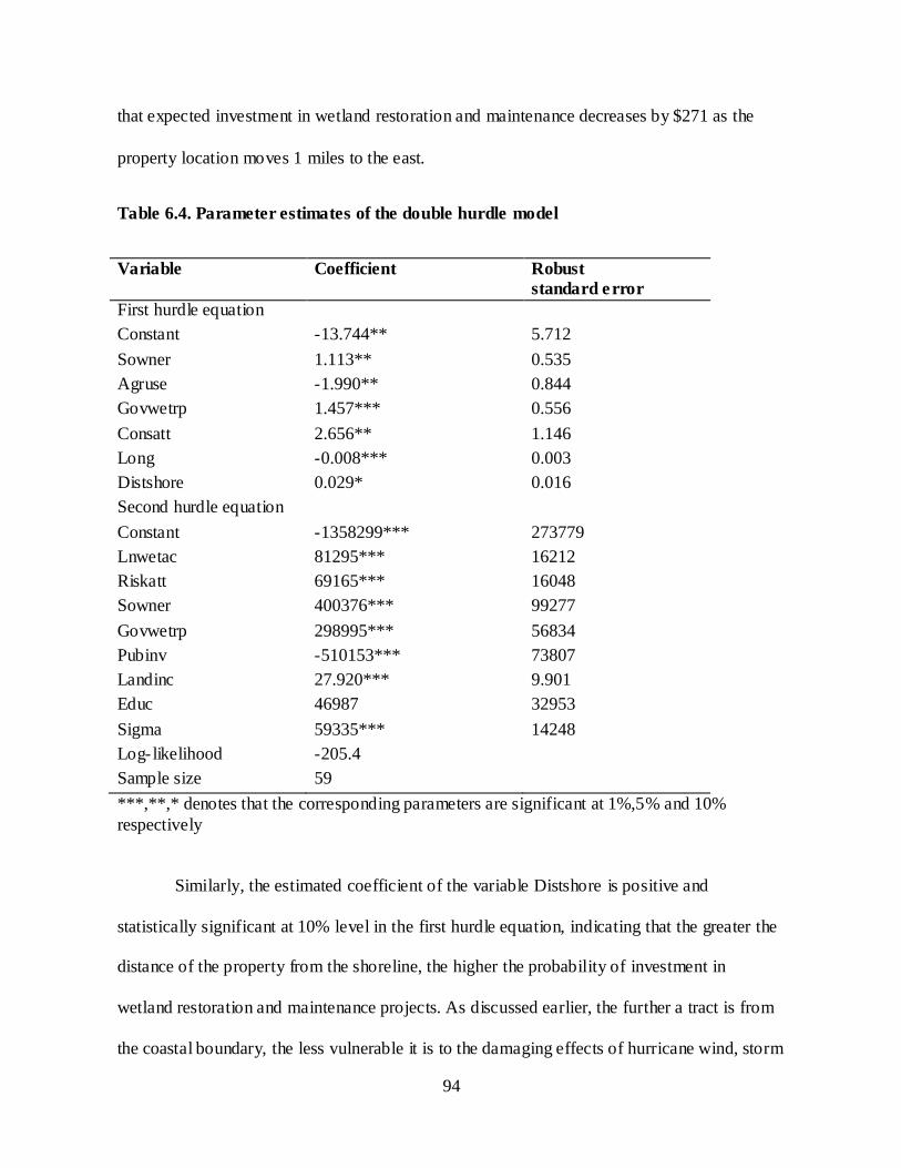
94

that expected investment in wetland restoration and maintenance decreases by $271 as the

property location moves 1 miles to the east.

Table 6.4. Parameter estimates of the double hurdle model

Variable Coefficient Robust

standard error

First hurdle equation

Constant -13.744** 5.712

Sowner 1.113** 0.535

Agruse -1.990** 0.844

Govwetrp 1.457*** 0.556

Consatt 2.656** 1.146

Long -0.008*** 0.003

Distshore 0.029* 0.016

Second hurdle equation

Constant -1358299*** 273779

Lnwetac 81295*** 16212

Riskatt 69165*** 16048

Sowner 400376*** 99277

Govwetrp 298995*** 56834

Pubinv -510153*** 73807

Landinc 27.920*** 9.901

Educ 46987 32953

Sigma 59335*** 14248

Log- likelihood -205.4

Sample size 59

***,**,* denotes that the corresponding parameters are significant at 1%,5% and 10%

respectively

Similarly, the estimated coefficient of the variable Distshore is positive and

statistically significant at 10% level in the first hurdle equation, indicating that the greater the

distance of the property from the shoreline, the higher the probability of investment in

wetland restoration and maintenance projects. As discussed earlier, the further a tract is from

the coastal boundary, the less vulnerable it is to the damaging effects of hurricane wind, storm

95

water surges, and other weather related factors. This, in turn, lowers the risk associated with

the decision to invest and may increase the likelihood of investing in such projects.

Furthermore, tracts that are located close to the shore line are generally dominated by salt

marshes and they are less productive than tracts located further from the shore, which are

dominated by fresh marshes, perhaps making them less attractive as investment candidates.

The marginal effect of this variable is positive and significant at the 1% level. It shows that

the probability of investment increases by 0.6% as the property‟s distance from the shore

increases by 1 mile. The unconditional marginal effect shows that investment in wetland

restoration and maintenance will increase by $1,067 as the property distance from the shore

increases by 1 mile.

Past studies have found ownership structure to be a significant influence on the

decision to invest in soil conservation (Soule et al., 2000); Featherstone and Goodwin, 1993;

Norris and Batie, 1987), forestry improvements ( Dhakal et al.,2008), and decisions to

participate in government forestry assistance programs (Nagubadi et al., 1996 ). In this study,

the impact of the ownership structure was captured using a dummy variable (Sowner) that

was equal one if the landowner was a sole-owner and 0 otherwise. The estimated coefficient

of this variable was positive and significant at the 5% level in the first hurdle, implying that

landowners who are sole-owners are more likely to invest in wetland restoration and

maintenance than other landowners. The marginal effect of this variable indicates that sole-

owners are 23% more likely to invest privately in wetland restoration and maintenance. In

addition, the coefficient of Sowner is positive and significant at the 1% level in the second

hurdle equation, implying that landowners who are sole-owners are not only more likely to

invest, but they also invest more than owners with other types of ownership structures. The

96

unconditional marginal effect indicates that sole-owners privately invest $103,405 more in

wetland restoration and maintenance activities than other landowners. Conditional on the

investment decision, sole-owners are found to invest $155,356 more in wetland restoration

and maintenance than other landowners.

Table 6.5. Marginal Effects for the Double Hurdle Model

Variable

Probability

Conditional Investment

Unconditional Investment

Lnwetac 25094*** 9454***

(5708.48) (345.21)

Riskatt 21350*** 8043***

(5651.14) (341.74)

Sowner 0.228 155356 103405

n/a n/a n/a

Agruse -0.290 -63139

n/a n/a

Govwetrp 0.332 125968 136470

n/a n/a n/a

Consatt 0.545*** 96528***

(0.1374) (7172)

Long -0.0015*** -271.28***

(0.00034) (18.24)

Distshore 0.006*** 1067.4***

(0.00194) (84.4)

Pubinv -121865 -61375

n/a n/a

Landinc 8.620** 3.25***

(3.359) (0.203)

Educ 14504 5464***

(10998.5) (665.11)

Note: Standard errors are in parentheses ***,**,* denotes that the corresponding parameters are significant at 1%,5% and 10% respectively,

The estimated coefficient for landowner attitudes toward wetland restoration and

maintenance (Consatt) was positive and statistically significant at the 5% level in the first

hurdle equation, indicating that landowners who value wetland restoration issues are more

97

likely to invest in coastal wetland restoration. The marginal impact of this variable suggests

that a 1 unit increase in the conservation attitude index increases the probability of investment

by 55% and increases the expected level of investment by approximately $96,528. Langpap

(2004) found conservation attitudes to be an important factor in private landowner decisions

to participate in incentives programs. Gelso et al. (2008) also found that farmer attitudes

toward conservation and environmental regulation have a significant impact on the perceived

costs associated with the presence of wetland areas on their farmlands. However, Ervin and

Ervin (1982) found no statistical evidence that conservation attitudes influence the decision to

invest in soil conservation.

The double hurdle estimation shows that landowners who are using part of their

properties for agricultural activities are less likely to invest in wetland restoration projects,

with the coefficient of the dummy variable (Agruse) being negative and significant at the 5%

level in the first hurdle equation. As discussed with respect to the Tobit model, this negative

relationship between the use of a land tract for agricultural production and the probability of

wetland investment is not surprising. Several factors can explain this negative correlation,

including the lack of farming income from wetland areas, competition for private capital

between agriculture production and wetland restoration, and the costs involved in changing

operational focus. The results of this study are similar to the findings of Royer (1987), where

engagement in farming activities was negatively related to reforestation investment. The

marginal effect value of this variable implies that landowners who are using their properties

for agricultural production have, on average, a 29% smaller chances of investing in wetland

restoration and maintenance than other landowners, ceteris paribus. The unconditional

98

marginal effect shows that landowners who use part of their landholdings for agriculture

production invest $63,139 less on wetland restoration and maintenance than other landowners.

In contrast to the Tobit model results, participation in government-sponsored wetland

restoration programs (Govwetrp) had a positive effect on the probability of investment and the

level of investment in the double hurdle model, with the estimated coefficient of Govwetrp

being positive and statistically significant at the 1% level in both hurdles. This result supports

the hypothesis that government wetland restoration programs have stimulated at least some

private wetland investment in coastal Louisiana. The marginal effect indicates that

landowners enrolled in wetland restoration programs have a 33% higher probability of

investing in wetland restoration and maintenance. The unconditional marginal effect shows

that landowners who were enrolled in wetland restoration programs invested $136,470 more,

on average, than other landowners. Conditional on having made the decision to invest,

landowners who are enrolled in wetland restoration programs invest $125,968 more than other

landowners. These results are similar to those found in other studies. For example, Hagos

and Holden (2006) studied the influence of public programs on the household‟s investment in

soil conservation in northern Ethiopia, and found that participation in public programs

stimulated investment in soil conservation. In another instance, Featherstone and Goodwin

(1993) used a Tobit model and found that participation in government programs had a

positive effect on farmer decisions to invest in soil conservation.

The estimated coefficient of the public investment dummy variable (Pubinv) was

negative and highly significant in the second hurdle equation, indicating that receiving public

financial assistance results in lower private investment, thus signaling a substitution

relationship between public and private capital. The marginal effects show that landowners

99

who use public investments to conduct wetland restoration and maintenance activities invest

$61,375 less than landowners who did not receive public investments. Conditional on

investing, landowners who use public investment invest $121,865 less on wetland restoration

and maintenance than other private landowners. This result is similar to Zhang and Flick

(2001), who found that forest landowners receiving cost sharing subsidies invested less of

their own capital in forest replanting. These authors also concluded that there was a

substitution effect between public funds and private capital.

Risk attitude was found to play an important role in the level of private investment

made by the landowner. The coefficient of this variable (Riskatt) was positive and statistically

significant at the 1% level, implying that the more risk averse the landowners, the lower the

investments will be in wetland restoration and maintenance. Both the conditional and

unconditional marginal effects for the risk attitude variable were statistically significant at the

5% level (see Table 6.5). The unconditional marginal effect indicates that a 1 unit increase in

the risk attitude score (in other words, becoming less risk averse) leads to an $8,043 increase

in the level of private investment. The conditional marginal effect of this variable shows that a

1 unit increase in the risk attitude score leads to $21,350 increase in the level of investments

for the landowners who have already made the investment decision. Figure 6.1 presents the

predicted wetland investments for various levels of risk aversion, holding all other variables

constant at their means. The predicted wetland investment ranges from $1,703 for a highly

risk averse landowner to $46,573 for a highly risk taking landowner. Therefore, risk aversion

decreases the expected level of wetland investment. This negative relationship between risk

aversion and investment has been documented in other studies that examined similar decision

making problems (Ervin and Ervin, 1982; Shapiro, 1992; Hagos and Holden, 2006; Benitez el

100

al., 2006; Goldstein et al., 2006; Stordal et al., 2007; Abadi Ghadim et al., 2005; Isik and

Khanna, 2003).

Figure 6.1 Predicted wetland investments associated with various levels of risk attitudes.

The coefficient of the wetland property size (lnwetac) was positive and statistically

significant in determining the level of investment (the second hurdle equation), indicating that

larger wetland properties generally experience higher levels of investment. Furthermore, the

coefficient of the wetland property size variable in the Tobit model was approximately 64%

lower than the estimated coefficient of wetland size in the double hurdle model. This

divergence between the two models exemplifies the degree of bias that can arise when an

intrinsically two-stage decision process is modeled as a single process. The conditional

marginal effect of wetland size suggests that a 1% increase in property size will lead to a $250

increase in the level of investment in restoration and maintenance, while the conditional

marginal effect for the Tobit model shows that a 1% increase in size increases the level of

investment by $299 (or approximately 20% more than the corresponding conditional

$0

$10,000

$20,000

$30,000

$40,000

$50,000

1 2 3 4 5 6 7 8 9 10

Risk attitude level

Predicted wetland investments

101

marginal effect reported for the double hurdle model). As a comparison, the literature reported

mixed results regarding the relationship between investment and the property size. Some

studies found that property size had significant positive effects on investment decisions

(Norris and Batie, 1987; Soule et al., 2000); Dhakal et al., 2008). Other studies, however,

found no significant relationship between property size and investment decisions (Ervin and

Ervin, 1982; Featherstone and Goodwin, 1993; Romm et at., 1987; Hagos and Holden, 2006;

Zhang and Flick, 2001). The result of double hurdle estimation in this study, however, clearly

indicates that property size has positive effects on the investment decisions for private

landowners.

The coefficient of the land income variable (Landinc) was positive and statistically

significant in the second hurdle equation, indicating that landowner income plays an

important role in determining the level of private investment in wetland restoration and

maintenance, with more productive properties (in terms of income) receiving higher levels of

private investment. This positive relationship between income and investment was reported in

a number of other studies (Norris and Batie, 1987; Romm et al., 1987; Zhang and Flick,

2001), but Featherstone and Goodwin (1993) did not find a relationship between total farm

income and soil conservation investments. The marginal effects reported in Table 6.5 show

that a $1 increase in income from wetland-based activities resulted in a $3.25 increase in the

level of investment for all landowners, and a $8.62 increase for those landowners who had

already made previous investments.

Finally, the estimated coefficient of the education variable (educ) was positive but

statistically insignificant. The unconditional marginal effect was significant and shows that a

move from one education category to the next highest category would lead to a $5,464

102

increase in the level of investment. For example, a respondent who has completed college will

invest $5,464 more in wetland restoration projects if he/ she has some college education (but

never completed it). On the other hand, the conditional marginal effect was larger in

magnitude, but not statistically significant. Previous studies have found education to be a

significantly positive influence on the level of investment in technology adoption (Saha et al.,

1994) and soil conservation (Ervin and Ervin, 1982; Norris and Batie, 1987; Hagos and

Holden, 2006).

One way of interpreting the estimated double hurdle model is by categorizing

landowners into two groups. The first group, landowners who do not cross the first hurdle

equation, may never invest in wetland restoration and maintenance under any circumstances.

The second group, landowners who pass the first hurdle, are potential investors. This second

group has two choices: a) invest in wetland restoration and maintenance (positive value of the

dependent variable) or b) do not invest in wetland restoration and maintenance (zero value of

the dependent variable). Therefore, the estimated double hurdle model can be used to predict

the probability that an individual landowner would fall in one of the two categories.

Consequently, looking at the common characteristics of the landowners in each category may

be of interest when it comes to discussing the policy implications of landowner behavior. The

probability that a landowner will not invest in wetland restoration and maintenance can be

expressed as follows:

(50)

where is a vector of the estimated parameters of the variables that are included in the first

hurdle equation. Equation (50) was estimated for all the landowners who did not invest in

103

wetland restoration and maintenance at the time the survey was taken. The predictive results

(see Figure 6.2) show that most landowners have a high probability of never investing in

wetland restoration projects. More specifically, the histogram shows that 85% of the

landowners who did not invest in wetland restoration projects at the time of the survey have

probabilities in excess of 0.5 that they will never invest in wetland restoration projects. The

results also show that, on average, the probability that a landowner in this group would never

invest in wetland restoration and maintenance was 0.81.

Figure 6.2: Histogram of predicted probability of no investment in wetland restoration

and maintenance

Similarly, we can use the double hurdle model to look at probability distributions for

landowners who are potential investors. The probability that a landowner will invest in

wetland restoration and maintenance is:

(50)

104

where is the vector of the estimated parameters of the variables that are included in the first

hurdle equation. Equation (50) was estimated for all landowners in the sample who reported

investing in wetland restoration projects at the time of the survey, and a frequency histogram

of the results is presented in Figure 6.3. The results indicate that only 46% of the landowners

who are potential investors have probabilities of investment higher than 50%. Put another

way, the majority of the landowners in the group of potential investors have probabilities of

investment lower than 50% based on the estimated double hurdle coefficients.

Figure 6.3: Histogram of predicted probability of investment in wetland restoration and

maintenance

105

6.4 Model Selection

The results of the Tobit and double hurdle models presented in the previous sections

show that both models adequately represented the collected data. However, comparisons of

the two models suggest that the double hurdle model might better explain the data (compared

to the Tobit model) due to a larger number of significant parameters. This hypothesis can be

tested by: a) estimating a Tobit model with only the variables found in the second hurdle of

the double hurdle model (the result of this restricted Tobit model is presented in Appendix C )

using a likelihood ratio test for the null hypothesis that the univariate Tobit is superior to the

double hurdle model. The resulting likelihood ratio statistic was 2(229.5-205.4)=48.2 with a

chi-square distribution and 7 degrees of freedom. This result indicates that the Tobit model

specification can be rejected in favor of the double hurdle model specification at the 5% level

of significance, or that landowners make private wetland restoration and maintenance

investment decisions in a sequential manner by first deciding whether to invest and then

deciding how much to invest.

While the Likelihood ratio (LR) test shows that the double hurdle model outperforms

the Tobit model, the double hurdle model is preferable to the Tobit model for other reasons,

too. For example, several variables, including risk attitude (Riskatt), are not statistically

significant in the Tobit model, but they are significant in the double hurdle model. In part,

this leads to the double hurdle model‟s better explanatory power.

Existing literature suggests that risk attitude plays an important role in investment

decisions (Ervin and Ervin, 1982; Shapiro, 1992; Hagos and Holden, 2006; Benitez el al.,

2006; Goldstein et al., 2006; Stordal et al., 2007; Abadi Ghadim et al., 2005; Isik and

Khanna, 2003; Saha et al., 1994; Koundouri et al., 2006). The majority of these studies found

106

a negative relationship between risk aversion and the level of investment. Results of the

double hurdle estimation are in line with these findings. The result of the Tobit model,

however, did not show that risk aversion significantly influenced the landowner‟s investment

decision.

Previous findings on the role of income on investment decisions are inconsistent.

Some studies found income to be an important factor in the investment decision (Norris and

Batie, 1987; Zhang and Flick, 2001; Romm et al., 1987), while others studies did not

(Featherstone and Goodwin, 1993). The result of the double hurdle model suggests that

income significantly influences the level of investment decision. This result is in line with the

results of most previous studies, and lends support to the double hurdle model as the best fit to

the data. On the other hand, the results of the Tobit model do not show that income affects

investment decisions of the landowners.

Participation in government programs has been found to influence the farmers‟

decisions to invest in soil conservation (Featherstone and Goodwin, 1993) and reforestation

investment ( Zhang and Flick, 2001 ). Two variables were used to capture the participation

decisions of the landowners in this study – Govwetrp and Pubinv. The coefficients of these

two variables are statistically significant in the double hurdle model, but not in the Tobit

model. This is additional evidence that the double hurdle model outperforms that Tobit model,

which in return emphasizes the importance of the first hurdle in the decision process.

It was hypothesized that the more positive the attitudes toward wetland restoration

issues, the more likely that landowners would invest in wetland restoration and maintenance.

This hypothesis is supported by both the estimated double hurdle model and the Tobit model.

107

The coefficient of the Consatt variable is positive and significant at 1% and 10% levels of

significance respectively. The result of the double hurdle model shows that landowners‟

attitudes toward wetland restoration influence only the landowners‟ decisions about whether

to invest but not the level of investment. This is the reason for including this variable only in

the first hurdle equation. Our findings are in line with the results of the study by Langpap

(2004).

In summary, the double hurdle model statistically outperformed the Tobit model, was a

better explainer of the collected data, and conformed to the majority of findings in related

research areas. The next, and final, chapter uses the results from the double hurdle model in

support of a discussion examining the implications of the modeling for efforts to promote the

use of private investment in coastal wetland restoration and maintenance.

108

CHAPTER 7

CONCLUSIONS AND POLICY IMPLICATIONS

Encouraging private wetland landowners to invest in wetland restoration and

maintenance activities can be a challenging task. First, any decision to invest in restoration

and maintenance is subject to a high level of uncertainty associated with climate change,

changes in wetland regulatory policy, and changes in restoration technologies, Second, the

majority of the benefits associated with wetland restoration and maintenance activities are

enjoyed by the public rather than private landowners themselves, thereby presenting, at least

partly, a public goods barrier to individual action. This dissertation developed a theoretical

model of the landowner‟s decision making process in the face of uncertainty and relatively

high wetland restoration costs. The conditions under which landowners would invest were

derived under assumptions of risk aversion and relatively high fixed and variable costs. The

validity of the theoretical model was tested using survey responses from 75 private wetland

landowners in coastal Louisiana. Two econometric models (Tobit and double hurdle) were

estimated to determine the importance of various factors, including risk aversion, on the

probability and the level of private coastal wetland investments.

The results of the survey data showed that the vast majority of landowners considered

the costs of wetland restoration and the uncertainty surrounding future benefits and costs of

wetland restoration projects as the major factors deterring wetland restoration in coastal

Louisiana. The survey respondents considered changing government policies and shifting

environmental conditions as major sources of uncertainty. Overall, the majority of landowners

were found to be risk averse, an observation that partly explains the respondent‟s focus on

109

uncertainty and highlights the fact that uncertainty and restoration costs play important roles

in the decision to invest in wetland restoration and maintenance activities.

The Likelihood Ratio (LR) test was employed to test the null hypothesis that the Tobit

was superior to the double hurdle model. The result of the LR test indicates that the Tobit

model specification can be rejected in favor of the double hurdle model specification, thus

suggesting that landowners make their investment decisions in a sequential, two-step process.

First, landowners decide whether to invest in wetland restoration and maintenance, and

second, they decide on how much to invest. The double hurdle model conformed closely to

both the theoretical expectations and previous empirical research concerning the importance

of various factors in the decision to invest in wetland restoration and maintenance. For

example, several variables, including risk attitudes of the landowners and land income were

not statistically significant in the Tobit model, but they were highly significant in the double

hurdle model.

The role of risk in landowner decisions was shown to arise from at least two sources:

the varying risk attitudes among landowners and the physical risk factors associated with the

location of the wetland property. More specifically, risk aversion decreased the expected level

of restoration and maintenance, and the physical risk factors associated with the location of

the wetland property, and high restoration costs, decreased the likelihood of investment.

These relationships are evident in the geographic dispersion of investments, where

landowners who own/manage properties that are located in the eastern part of the state and

located close to the shore line (highly vulnerable areas) being less likely to invest in wetland

restoration and maintenance projects than other landowners.

110

Wetland property size was also an important factor that helped determine whether a

landowner would invest in wetland restoration and maintenance. Landowners with larger

wetland properties invested more in wetland restoration and maintenance activities than other

landowners. The results also indicated that landowners who used at least part of their

properties for agriculture production were less likely to invest in restoration projects. A

couple of reasons can be proposed for this finding, including the potential for lost farm

incomes due to wetlands – either because of direct resource-use competition or competition

for scarce fixed and variable cost capital – or the diversion of managerial focus from

production to preservation. The results also show that landowners who are sole-owners are

not only more likely to invest in wetland restoration and maintenance, but they also invest

more in these projects. Landowner‟s attitudes toward wetland conservation had a positive

influence on the decisions to invest in wetland restoration and maintenance, with positive

attitudes toward wetland conservation increasing the probability of investment.

Participation in government-sponsored wetland restoration programs was a very

important determinant of a landowner‟s investment decisions. Landowners who participate in

government-sponsored wetland restoration programs have higher probabilities of privately

investing in wetland restoration and they make larger investments than other landowners. At

the same time, private investment expenditures in wetland restoration projects are lower for

landowners receiving public financial assistance, which suggests a substitution effect between

public and private capital.

Finally, the results of the double hurdle model showed that income is also important

determinants of a landowner‟s decision to invest in wetland restoration and maintenance.

Total household income derived from activities on the wetland property had a positive

111

influence on the investment decision, with higher income households having higher levels of

investment. Education also had a positive effect on the landowner‟s decision regarding the

level of wetland investment but it was statistically insignificant at 10% level of significance,.

The result of this modeling effort also highlighted the difference between the marginal

effects obtained by averaging the partial effects across the sample (average marginal effects)

and the marginal effects obtained at the sample means. In general, average marginal effects

for the Tobit model were approximately 7 to 8 times more than the marginal effects computed

at the sample mean. This result raises a serious question about which marginal effect should

be used in an analysis. For example, if the average marginal effects across the sample are the

correct ones, then using the marginal effects at the sample means can seriously underestimate

the effects of the explanatory variables and lead to erroneous conclusions. The opposite is true

if the marginal effects at the sample mean are the correct ones. While the literature contains

only limited discussions of this topic, and is still inconclusive about which type of marginal

effects should be used, several authors have advocated the use of average marginal effects for

nonlinear models and models with discrete variables (Greene 2003,Wooldridge 2002, Papke

and Wooldridge 2008, Bartus 2005). Therefore, only the average marginal effects for the

double hurdle model were reported, and all the discussions of the model results were done in

terms of the average marginal effects.

Once estimated, the double hurdle model was used to predict the probability of zero

future investments in wetland restoration and maintenance projects for all landowners in the

sample who did not undertake any wetland restoration projects. The results indicate that 85%

of the landowners who did not invest in wetland restoration projects at the time of the survey

have probabilities in excess of 0.5 that they will never invest in wetland restoration projects.

112

This finding supports the anecdotal evidence that the vast majorities of landowners are not

only not planning to invest in wetland restoration and maintenance, but that the idea of doing

so does not even occur to them.

The results presented in this dissertation have potentially important implications for

the design of policy instruments to encourage private wetland restoration efforts in coastal

Louisiana. First, policies need to consider the effects of risk aversion, and uncertainty on a

landowner‟s decisions to invest in wetland restoration projects. Failure to do so will not only

lead to overestimating the participation rates in a program, but it will also lead to

underestimating the size of the needed incentive payments for participation and the expected

costs of the policy instruments. Therefore, incorporating the effects of risk aversion, and

uncertainty into the benefit-cost analysis of the proposed policy may provide more realistic

assessment of how a wetland restoration policy will perform in the future.

Another result with strong policy implications concerns the current and future role of

publically-funded restoration programs. Landowners who participate in government-

sponsored wetland restoration programs are more likely to invest in wetland restoration and

maintenance and make more private investments than landowners who have no experience

with the government programs. This suggests that the existing programs in the coastal zone

such as Wetlands Planning, Protection and Restoration Act (CWPPRA), and Coastal Wetland

Reserve Program (CWRP) have been effective in introducing restoration technology to

landowners and in encouraging them to take a more active role in the stewardship of their

land. Coupled with the result that a landowner‟s attitudes toward wetland conservation have a

positive influence on the probability of investing, an argument can be made in favor of

expanded education programs concerning the benefits of wetland conservation and restoration

113

activities. At the same time, however, there was a distinct public- for-private capital

substitution effect when examining landowners who received some form of financial

assistance in conducting restoration projects. While this substitution effect is not surprising, it

does imply that the size of, and rules governing, financial assistance programs needs to be

closely considered so that they do not have the perverse effect of reducing overall private

investment.

The results of the modeling effort clearly showed a competitive relationship between

agricultural production and wetland restoration. While policies similar to the Wetland

Reserve Program – which provides financial and technical support for landowners to protect

and restore wetland areas on their properties – would be one way to reduce this competition,

other avenues need to be explored to increase the revenue generating capability of wetlands,

particularly those in agricultural areas. In fact, because the total amount of household income

derived from activities on the wetland property was found to have positive influence o n the

level wetland investment, one could expect wetland owners to welcome that enhance the

income generation capability of wetland properties. For example, under the North American

Wetlands Conservation Act (NAWCA), landowners can receive financial support to

undertake waterfowl habitat improvement projects. The survey data shows that waterfowl

hunting was the primary land use among the survey respondents. Therefore, the expansion of

programs such as NAWCA should provide additional incentives for private restoration

activities in the coastal zone.

Variations in wetland investments across the characteristics of the landowners and

their landholdings have policy implications with regard to the design and implementation of

wetland restoration programs that seek to encourage private actions. For example, results of

114

the double hurdle model suggests that any program will be more effective if it targets

landowners who are more educated, own large wetland properties, are sole-ownership

organized, are not engaged in agricultural production, and have properties that are located

inland and in the western part of state. Such a policy, if correctly structured and implemented,

could lead to high participation rates and significant private investments. For example, we

used the parameter estimates of the double hurdle model to estimate the total amount of

private investment that has been expended by all landowners in the analysis. We find that the

estimated total level of investment for all 59 landowners over the last ten years is

approximately $2,629,991. On average, each landowner invests about $44,576 in wetland

restoration and maintenance activities over the last ten years. Extrapolating that level of

investment to all landowners in the sample frame, the expected level of private investment in

wetland restoration and maintenance is $7,481,258 for the ten year period.

In the absence of targeted wetland restoration programs, wetland investments might

not occur in coastal areas where wetland restoration projects are thought to be needed the

most (i.e., areas with high wetland loss rate). If the objective of the wetland policy is to

maximize investments in high-risk areas, then publicly-funded projects may be a better

approach. Alternatively, it may be possible to design a program, or separate programs, that

would address the unique characteristics of the wetland restoration problems on the opposite

sides of the state.

Given the magnitude and scope of the problem in coastal Louisiana, the best strategies

for addressing wetland loss should include cooperation between all interested parties,

jncluding private landowners, local communities and their citizens, and government officials.

Private landowners control the vast majority of wetlands in the coastal zone, but they have

115

very limited private capital and their investment decisions have limited effects in the absence

of existing large scale public restoration projects. Similarly, there are limited public funds to

completely address the issue of wetland loss in Louisiana‟s coastal zone, and the majority of

public restoration projects will either affect or be implemented on private properties. As a

result, the cooperation of private landowners, and the coordination of their private investment

decisions with public restoration projects, are necessary for any successful wetland restoration

effort. Wetland restoration programs can be more effective if they target the participation of

private landowners in areas that are actively being addressed by public restoration projects.

Furthermore, these wetland restoration programs will be most effective if they are designed to

encourage greater coordination of investment decisions of adjacent landowners and

landowners in close geographic areas.

.

116

REFERENCES

Abadi Ghadim, A.K., D.J. Panell., and M.P. Burton. 2005. Risk, uncertainty, and learning in

adoption of a crop innovation. Agricultural Economics 33:1-9. Alig, R.J. 1986. Econometric analysis of the factors influencing forestry acreage trends in the

Southeast. Forestry Science, 32(1):119-134.

Amemiya, T. 1984. “Tobit models: A survey.” Journal of Econometrics 24: 3-61. Antle, J.M. 1983. Incorporating risk in production analysis. American Journal of Agricultural

Economics 65:1099–1106

Arabmazer, A., and P. Schmidt. 1982.An investigation into the robustness of the Tobit estimator to nonnormality. Econometrica 50:1055-1063

Arabmazer, A., and P. Schmidt. 1981.Further evidence on the robustness of the Tobit estimator to hetroskedasticity. Journal of Econometrics 17:253-258

Arrow, K.J. and A.C. Fisher. 1974. Environmental preservation, uncertainty, and irreversibility.” Quarterly Journal of Economics 88:312-319.

Arrow, K.J. 1971. Essays in the theory of risk bearing. Chicago: Markham Publishing.

Bard, S.K., and P.J. Barry. 2001.Assessing farmers‟ attitudes toward risk using „closin-In‟ Methods. Journal of agricultural and resource Economics 26:248-260.

Baron, R. A., and Byrne, D. (1981). Social psychology: Understanding human interaction

(3rd ed.). Boston: Allyn & Bacon. Barras, J.A., Bernier, J.C., and Morton, R.A., 2008, Land area change in coastal Louisiana--A

multidecadal perspective (from 1956 to 2006): U.S. Geological Survey Scientific Investigations Map 3019, scale 1:250,000, 14 p. pamphlet

Bartus, T. 2005. Estimation of marginal effects using margeff. The Stata Journal 5(3):309-329

Benitez, P. C., T. Kuosmanen., R. Olschewski., and G.C. Van Kooten. 2006. Conservation

payments under risk: A stochastic dominance approach. American Journal of Agricultural Economics 88:1-15.

Blundell, R., and C. Meghir. 1987. Bivariate alternatives to the univariate Tobit model. Journal of Econometrics 34:179-200.

117

Boesch, D.F., M.N. Josselyn, A.J. Mehta, J.T. Morris, W.K. Nuttle, C.A. Simenstad, and D.J.P. Swift. 1994. Scientific assessment of coastal wetland loss, restoration and management

in Louisiana. Journal of Coastal Research 20:1-103

Burke, W.J. 2009. Fitting and interpreting Cragg‟s Tobit alternative using Stata. The Stata Journal 9(4):584-592

Bulte, E., D.P.Van Soest., G.C. Van Kooten., and R. A. Schipper. 2002. Forest conservation in Costa Rica when nonuse benefits are uncertain but rising. American Journal of Agricultural

Economics 84(1):150–160. Caffey, R.H. and M. Shexnayder. 2003. Coastal Louisiana and south Florida: A comparative

wetland inventory. Draft Fact Sheet. Louisiana State University.

Caffey, R.H. 2005. Why is Louisiana losing its coastal wetlands and how much have been lost? Louisiana sea grant hurricane resources recovery website, FAQ,

Capozza, D.R. and Y. Li. 1994. The intensity and timing of investment: the case of land. American Economic Review 84(4):889-904.

Cameron, A.C., and P.K. Trivedi.2009. Microeconometrics using Stata. College Station, TX: Stata Press.

Capozza, D.R. and G.A. Sick. 1994. The Risk structure of land markets. Journal of Urban

Economics 35:297-319. Capozza, D.R. and R. Helsley. 1990. The Stochastic city. Journal of Urban Economics

28:187-203

Capozza, D.R. and Y. Li. 1994. “The intensity and timing of investment: The Case of Land.” American Economic Review 84(4):889-904.

Capozza, D.R. and G.A. Sick. 1994. The Risk structure of land markets. Journal of Urban Economics 35:297-319.

Cardona, H. 1999. Analysis of policy alternatives in implementation of coastal nonpoint pollution control program for agriculture, PhD Thesis, Department of Agricultural Economics

and Agribusiness, Louisiana State University, Baton Rouge.

Carey.J M; and D. Zilberman.2002. A model of investment under uncertainty : Modern Irrigation technology and emerging markets in water. American Journal of agricultural economics 84: 171-183

Carroll, J., S.McCarthy., and C. Newman.2005. An econometric analysis of charitable

donations in the republic of Ireland. The Economic and Social Review 36(3):229-249.

118

Churchill, G.A. 1995.Marketing research: methodological foundations. Chicago: The Dryde n Press.

Coastal Wetlands Planning, Protection and Restoration Act (CWPPRA ). 2006. A response to

Louisiana‟s land loss. Coastal Protection and Restoration Authority( CPRA). 2007. Fiscal year 2008 annual plan:

ecosystem restoration and hurricane protection in coastal Louisiana.

Cragg, J.G. 1971. Some statistical models for limited dependent variables with application to the demand for durable goods. Econometrica 39(5): 829-844

Dhakal, B., H. Bigsby.,and R. Cullen. 2008. Determinants of forestry investment and extent of forestry expansion by smallholders in New Zealand. Review of Applied Economics 4:65-76.

Day, J. W., Jr., J. Barras., E. Clairain, J. Johnston, D. Justic, G. P. Kemp, J.-Y. Ko, R. Lane, W. J. Mitsch,G. Steyer, P. Templet, and A. Yañez-Arancibia. 2005. Implications of global

climatic change and energy cost and availability for the restoration of the Mississippi delta. Ecological Engineering 24:253-265.

Dillman, D. 1978. Mail and telephone surveys: The total design method. New York: John Wiley and Sons.

Dixit, A.K. and R.S. Pindyck. 1994. Investment under uncertainty. Princeton, NJ: Princeton

University Press. Epstein,L.G.1980. Decision making and the temporal resolution of uncertainty. International

Economic Review 21(2):269-283.

Ervin, C A. and D. E. Ervin. 1982. Factors affecting the use of soil conservation practices: hypotheses, evidence and policy. Land Economics 58(3):277-292

Fausti, S and J. Gillespie. 2006. Measuring risk attitude of agricultural producers using a mail survey : how consistent are the methods. The Australian journal of agricultural and resource

economics, 50:171-188. Featherstone, A.M. and B.K. Goodwin. 1993. Factors influencing a farmer‟s decision to

Invest in long-term conservation improvements. Land Economics 69(1):67-81.

Feder,G., R.E. Just., and D. Zilberman.1985. Adoption of agricultural innovation in developing countries: A survey. Economic Development and Cultural Change 33:255-298.

Fisher, A. C., and W.M. Hanemann. 1990. “Option value: theory and measurement”, European. Review of Agricultural Economics 7(2): 167-180

119

Fisher, A.C., J.V. Krutilla and C.J. Cicchetti. 1972. The economics of environmental preservation: A theoretical and empirical analysis. American Economic Review 62:605-619.

Galloway, G., D. Boesch, and R. R. Twilley. 2009. Restoring and protecting coastal

Louisiana. Issues in Science and Technology, Winter 2009:29–38. Gelso, B.R., J.A. Fox.,and J.M. Peterson. 2008. Farmers‟ perceived costs of wetland: effects

of wetland size, hydration, and dispersion. American Journal of Agricultural Economics 90(1):172-185.

Geltner, D., T. Riddiough, and S. Stojanovic. 1996. Insights on the effect of land use choice: The perpetual option on the best of two underlying assets. Journal of Urban Economics

39:20–50.

Goldstein , J.H . G.C Daily. J. B. Friday. P.A, Matson.R. L, Naylor. and P,Vitousek. (2006). Business strategies for conservation on private lands: Koa forestry as a case study. Proceedings of the National Academy of Sciences 103: 10140-45.

Goodwin, B.K., and T.C. Schroeder.1994. Human capital, producer education programs, and

the adoption of forward pricing methods. American Journal of Agricultural Economics 76:936-947

Greene, W.H. 2003. Econometric analysis. 5th ed. Upper Saddle River, NJ: Prentice Hall

Gunjal,K., and B. Legault. 1994. Risk preferences of dairy and hog producers in Quebec. Canadian Journal of Agricultural Economics 43: 23-36.

Jenson, H.H., and S. T. Yen. 1996. Food expenditures away from home by type of meal. Canadian Journal of Agricultural Economics 44:67-80.

Hagos,F. and S. Holden. 2006. Tenure security, resource poverty, public programs and household plot level conservation investments in the highlands of north Ethiopia. Agricultural

Economics 34:183-196

Heimlich, R.E., K.D. Weibe., R. Claassen., D. Gadsy.,and R.M. House. 1998. Wetlands and agriculture: Private interests and public benefits. Resource Economics Division, E.R.S., USDA, agricultural economic report 765.10.

Henderson,J.E. 2007. Liability, institutions, and determinants of landowner access policies for

fee-based recreation on private lands. Ph.D. Dissertation, Department of Agricultural Economics and Agribusiness, Louisiana State University, Baton Rouge.

Henry, C. 1974. Investment decisions under uncertainty: The irreversibility effect, The American Economic Review, 64(6):1006-1012.

120

Hurd, M. 1979. Estimation in truncated samples when there is hetroskedasticity. Journal of Econometrics 11:247-258

Isik, M., and W. Yang. 2004. An analysis of the effects of uncertainty and irreversibility on

farmer participation in the conservation reserve program. Journal of Agricultural and Resource Economics 29(2):242-259

IsiK, M. and, M . Khanna.(2003) Stochastic technology, risk preferences and adoption of site-specific technologies. American Journal of Agricultural Economics 85:305-317.

Isik, M., M. Khanna, and A. Winter-Nelson. 2001. Sequential investment in site-specific crop management under output price uncertainty.Journal of Agricultural and Resource Economics

26: 212–29.

Jones, D., C. Cocklin and M. Cutting. 1995. Institutional and landowner perspectives on wetland management in New Zealand. Journal of Environmental Management 45:143-161.

Koundouri, P., C. Nauges., and V. Tzouvelekas.2006. Technology adoption under production uncertainty: theory and application to irrigation technology. American Journal of Agricultural

Economics 88(3):657-670. Kim, K., and J.P. Chavas. 2003. Technological change and risk management: An application

to the economics of corn production. Agricultural Economics 29:125-42.

Kline, J.,R.J. Alig., and R.L. Johnson. 2000. Fostering the production of non-timber services among forest owners with heterogeneous objectives. Forest Science 46:302-311.

Knapp, K.C., and L.J. Olson.1996. Dynamic resource management: intertemporal substitution and risk aversion. American Journal of Agricultural Economics 78:1004–1014.

Layva, J.C., J.A. Franco Martinez., and M.C. Gonzalez Roa. 2007. Analysis of the adoption of soil conservation practices in olive groves: the case of mountainous areas in southern Spain.

Spanish Journal of Agricultural Research 5(3):249-258.

LaDNR.1999. Coast 2050: Toward a sustainable coastal louisiana, Louisiana Coastal Wetlands Conservation and Restoration Task Force, La Dept. of Natural Resources. Baton Rouge, LA.

Lipton, D.W., K. Wellman., I.C. Sheifer., and R .F. Weiher. 1995.Economic evaluation of

natural resources: A handbook for coastal resource policymakers.NOAA coastal ocean program decision analysis series No. 5. NOAA coastal ocean office, Silver Spring, MD.

Maddala,G.,and F. Nelson. 1975. Specification errors in limited dependent variable models. Working paper 96, National Bureau of Economic Research. Cambridge, Mass.

121

McDonald, J.F., and R.A. Moffitt.1980. The uses of Tobit analysis. Review of Economics and Statistics 62:318-321.

Moffatt, PG.2005. Hurdle models of loan default. Journal of Operation Research Society

56:1063-1071. Nagubadi,V. K.T. McNamara.,W. L. Hoover., and W.L. Mills, Jr. 1996. Programs participation

behavior of nonindustrial forest landowners: A probit model. Journal of Agricultural and Applied Economics 28(2):323-336

Norris, P. E., and S. S. Batie. 1987. Virginia farmers‟ soil conservation decisions: An application of Tobit analysis. Southern Journal of Agricultural Economics 19(1):79-90.

Penning, M.E., and P. Garcia. 2001. Measuring producers‟ risk preference: a global risk-

attitude construct. American Journal of Agricultural Economics 83(4):993-1009 Papke,L.E., and J.M. Wooldridge. 2008. Panel data methods for fractional response variables

with an application to test pass rates. Journal of econometrics 145:121-133

Parks, P. J., and Kramer.1995. A policy simulation of wetlands reserve program. Journal of Environmental Economics and Management 28:223-240

Parks, P. 1993. Explaining Irrational land use: Risk aversion and marginal agricultural land. Journal of environmental economics and management 28:34-47

Paulsen,S. 2007. Investment in wetlands for pollution abatement under uncertainty. PhD Dissertation. Department of Economics, Swedish University of Agricultural Sc iences (SLU),

Uppsala.

Plantinga. A.J., R.N. Lubowski., and R.N. Stavins. 2002. Effects of potential land development on agricultural land prices. Journal of Urban Economics 52:561-581

Pratt, J. 1964. Risk aversion in the small and in the large. Econometrica 32: 122-136.

Purvis, A., W.G. Boggess, C.B. Moss, and J. Holt. 1995. Technology adoption decisions under irreversibility and uncertainty: An ex ante approach.” American Journal of Agricultural Economics 77:541–551.

Quigg, L.1993. Empirical testing of real option-pricing models. Journal of Finance

48(2):621-640. Romm, J., R. Tuazon.,C. Whashburn. 1987. Relating forestry investment to the characteristics

of nonindustrial private forestland owners in northern California. Forest Science 331:197-209

Royer, J.P. 1987. Determinants of reforestation behavior among southern landowners. Forest Science 33(3):654-667

122

Ryan, M., and C.D. Susman. 2003. Wetlands conservation in Louisiana: Voluntary incentives

and other alternatives, Journal of Environmental Law and Litigation 17: 441-495.

Saha, A., H.A. Love and R. Schwart. 1994. Adoption of emerging technologies under output uncertainty. American Journal of Agricultural Economics 76:836-846.

Schatzki, T. 2003. Options, uncertainty and sunk costs: an empirical analysis of the land use change. Journal of Environmental economics and management 46:86-105.

Schurle, B., and Tierney, W.I. 1990. A comparison of risk preference measurements with implications for extension programming, staff paper no. 91-6. Department of Agricultural

Economics, Kansas State University, Monhattan.

Soderqvist, T. 2003. Are farmers prosocial? determinants of willingness to participate in Swedish catchment-based wetland creation program. Ecological Economics 47:105-120.

Soule, M., A. Tegene and K.D. Wiere. 2000. Land tenure and the adoption of conservation practices. American Journal of Agricultural Economics 82(4):993-1005.

Straka,T.J., H.W. Wisdom.,and J.E. Moak. 1984. Size of forest holding and investment behavior of nonindustrial private owners. The Journal of Forestry 82(8):495-496.

Stordal, G. L,. J.B. Hardaker., and L.J. Asheim. 2007. Risk aversion and optimal forest

replanting : A stochastic efficiency Study. European journal of Operational Research 181:1584-92.

StataCorp. 2009. Stata Statistical Software: Release 11. College Station, TX: StataCorp LP.

Su, S-J. B., and S. T. Yen. 1996. Microeconometric models of infrequency purchased goods:

An application to household pork consumption. Empirical. Economics 21: 513-533. Tengene, A,. K.Wiebe., and B. Kuhn. 1999. Irreversible investment under uncertainty :

conservation easements and option to develop agricultural land. Journal of Agricultural Economics 50:203-219.

Thomas, A.C. 1987. Risk attitudes measured by the interval approach: a case study of Kansas Farmers . American Journal of Agricultural Economics, 69:1101-1105.

Tobin,J.1958. Estimation of relationships for limited dependent variables. Econometrica

26(1):24-36. Torkamani, J., and S. Shajari. 2008. Adoption of new irrigation technology under production

risk. Water Resources Management 22:229-237.

123

Winter-Nelson, A., and K. Amegbeto. 1998. Option values to construction and agricultural price policy: application to terrace construction in Kenya. American Journal of Agricultural

Economics 80:409–418.

Wiemers, E. and Behan, J. 2004. Farm forestry investment in Ireland under uncertainty. The Economic and Social Review 35:305-320.

Wooldridge, J.M. 2002. Econometric analysis of cross section and panel data. Cambridge, MA: MIT Press.

Zhang, D., and W.A.Flick.2001. Sticks, carrots, and reforestation investment. Land Economics 77(3):444-455

Zhao, J. and D. Zilberman. 1999. Irreversibility and restoration in natural resource

development. Oxford Economic Papers 51(July):559-573.

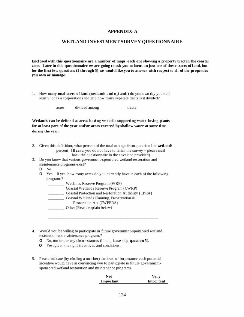
124

APPENDIX-A

WETLAND INVESTMENT SURVEY QUESTIONNAIRE

Enclosed with this questionnaire are a number of maps, each one showing a property tract in the coastal

zone. Later in this questionnaire we are going to ask you to focus on just one of these tracts of land, but

for the first few questions (1 through 5) we would like you to answer with res pect to all of the properties

you own or manage.

1. How many total acres of land (wetlands and uplands) do you own (by yourself,

jointly, or as a corporation) and into how many separate tracts is it divided?

________ acres div ided among ________ tracts

Wetlands can be defined as areas having wet soils supporting water -loving plants

for at least part of the year and/or areas covered by shallow water at some time

during the year.

2. Given this defin ition, what percent of the total acreage from ques tion 1 is wetland?

________ percent (If zero, you do not have to finish the survey – please mail

back the questionnaire in the envelope provided).

3. Do you know that various government-sponsored wetland restoration and

maintenance programs exist?

o No

o Yes – If yes, how many acres do you currently have in each of the following

programs?

________ Wetlands Reserve Program (WRP)

________ Coastal Wetlands Reserve Program (CWRP)

________ Coastal Protection and Restoration Authority (CPRA)

________ Coastal Wetlands Planning, Preservation &

Restoration Act (CWPPRA)

________ Other (Please exp lain below)

_______________________________________________________

4. Would you be willing to participate in future government-sponsored wetland

restoration and maintenance programs?

o No, not under any circumstances (If no, p lease skip question 5).

o Yes, given the right incentives and conditions.

5. Please indicate (by circling a number) the level of importance each potential

incentive would have in convincing you to participate in future government -

sponsored wetland restoration and maintenance programs.

Not Very

Important Important

125

General tax breaks

1---------2---------3---------4---------5

Cost-sharing assistance

1---------2---------3---------4---------5

Direct grants and subsidies

1---------2---------3---------4---------5

Temporary conservation easements

1---------2---------3---------4---------5

Permanent conservation easements

1---------2---------3---------4---------5

Expanded opportunities to use

wetlands in mitigation banking

(development offset)

1---------2---------3---------4---------5

Use of wetlands in carbon credit

programs

1---------2---------3---------4---------5

Other incentives (please explain)

1---------2---------3---------4---------5

___________________________________________________________

The next section of the questionnaire (questions 6 through 24) seeks information about one of the property

tracts that you own. If you look at the property maps, you will notice that each is labeled with a letter at

the top. Please choose the property tract that you have invested the most in with respect to wetlands

restoration/maintenance and answer the following questions with that s pecific property in mind. If you

have not invested in any of the property tracts, please choose the largest tract and ans wer the remaining

questions.

I am going to be ans wering the following questions with res pect to property

o Tract A

o Tract B

6. Do you still maintain ownership (solely, jointly, or other) in the tract?

o Yes – If yes, in what year did your ownership start? _______

o No – If no, what year did you stop owning the property? _______

IF YOU NO LONGER HAVE OWNERS HIP,

PLEAS E S KIP TO QUES TION 25.

7. How do you own the specific property tract?

o Sole ownership

o Joint ownership through a tenants -in-common arrangement

o Joint ownership through a corporation or trust

o Other (p lease exp lain )

________________________________________________________

8. If you maintain jo int ownership of the property, what percent of the tract do

you own?

_________ percent

126

9. What percent of your total 2008 household income came from surface (non-oil

& gas) activities taking place on the tract?

_________ percent

10. What percent of your total 2008 household income came from sub-surface (oil

& gas) activities taking place on the tract?

_________ percent

11. How many wetland acres have been lost on this tract of land due to erosion,

storms, or other environmental factors during the time you have owned it?

________ acres

12. How would you describe the overall condition of the wetlands within the tract?

o Poor

o Good

o Excellent

o I don‟t know

13. Please indicate (by circling a number) the level of importance each of the

listed activities has in the way the property tract is currently used.

Not Very

Important Important

Agriculture production

1---------2---------3---------4---------5

Timber production

1---------2---------3---------4---------5

Fur trapping, alligator hunting,

and/or egg collection

1---------2---------3---------4---------5

Waterfowl hunting

1---------2---------3---------4---------5

All types of fishing

1---------2---------3---------4---------5

Oil & gas activities

1---------2---------3---------4---------5

Other (p lease exp lain )

1---------2---------3---------4---------5

14. Is any part of this tract being leased out for activit ies in question 13?

o No Yes – If yes, how many acres are leased out? _______ acres

15. Which of the following best describes the current management of this property?

o Self-managed

o Managed using a hired service or employees

o Managed by a leaseholder

o Not being actively managed

o Managed by government personnel

16. If you were to sell the property tract today, what price do you think you might

receive?

127

$ ____________

17. Have any wetland maintenance or restoration activities ever been attempted on

this tract of land?

o No, not to my knowledge (please skip to question 22)

o Yes – If yes, what year d id they start? _______ year

Please estimate the total number of wetland acres that have been

restored or maintained on this tract of land over the last 10 years _______acres

18. What practices were used to restore or maintain the wetlands on this tract of

land? (Please check all that apply)

o Water control structures (gates, weirs, etc.)

o Vegetative plantings (trees or grasses)

o Nutrient/sediment traps (brush fences, terraces, etc.)

o Sediment, dredge or spoil usage

o Increased fresh water inputs to the property

o Other (p lease exp lain below)

_______________________________________________________

19. If you were involved in the decision to undertake restoration and maintenance

activities on this tract of land, please indicate (by circling a number) the level of

importance each of the listed reason was to your decision.

Not Very

Important Important

Availability of restoration

subsidies in the form of

monetary payments

1---------2---------3---------4---------5

Availability of restoration

subsidies in the form of

technical assistance

1---------2---------3---------4---------5

Desire to protect or enhance the

property market value

1---------2---------3---------4---------5


property‟s revenue generating

ability

1---------2---------3---------4---------5

Recent improvements in

restoration technology

1---------2---------3---------4---------5


ecological functions

1---------2---------3---------4---------5

Other (p lease exp lain below)

1---------2---------3---------4---------5

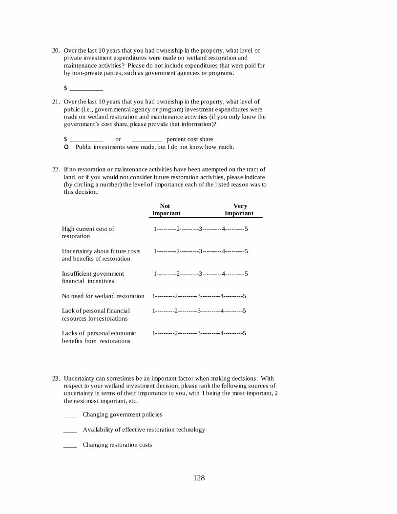
128

20. Over the last 10 years that you had ownership in the property, what level of

private investment expenditures were made on wetland restoration and

maintenance activities? Please do not include expenditures that were paid for

by non-private parties, such as government agencies or programs.

$ __________

21. Over the last 10 years that you had ownership in the property, what level of

public (i.e., governmental agency or program) investment expenditures were

made on wetland restoration and maintenance activities (if you only know the

government‟s cost share, please provide that information)?

$ __________ or _________ percent cost share

o Public investments were made, but I do not know how much.

22. If no restoration or maintenance activities have been attempted on the tract of

land, or if you would not consider future restoration activities, please indicate

(by circling a number) the level of importance each of the listed reason was to

this decision.

Not Very

Important Important

High current cost of

restoration

1---------2---------3---------4---------5

Uncertainty about future costs

and benefits of restoration

1---------2---------3---------4---------5

Insufficient government

financial incentives

1---------2---------3---------4---------5

No need for wetland restoration

1---------2---------3---------4---------5

Lack of personal financial

resources for restorations

1---------2---------3---------4---------5

Lacks of personal economic

benefits from restorations

1---------2---------3---------4---------5

23. Uncertainty can sometimes be an important factor when making decisions. With

respect to your wetland investment decision, please rank the following sources of

uncertainty in terms of their importance to you, with 1 being the most important, 2

the next most important, etc.

____ Changing government policies

____ Availability of effect ive restoration technology

____ Changing restoration costs

129

____ Shift ing environmental conditions

____ Others (please specify______________________________________)

24. If you consider uncertainty an important factor in your wetland investment decision,

please indicate your level of uncertainty in whether your investment will yield a

positive payoff by circling the appropriate number?

0---------1--------2-------3-------4--------5--------6-------7--------8--------9-------10

No uncertainty High uncertainty

This next question seeks information that will help us better understand your

attitudes concerning coastal wetlands restoration.

25. Please indicate how much you disagree or agree with each of the statements by

circling the appropriate number using the given scale:

Strongly Strongly

Disagree Agree

Restoration is important to

future generations

1----------2----------3----------4----------5

Restored wetlands protect

wildlife and/or fish habitat

1----------2----------3----------4----------5

Restoring wetlands

improves water quality and

reduces erosion

1----------2----------3----------4----------5

Restored wetlands provide

storm and flood protection

1----------2----------3----------4----------5

Restoring wetlands is a

waste of time and money

given the predicted

increases in sea level

1----------2----------3----------4----------5

In this next section we ask questions that will allow us to categorize your res ponses with

other survey participants.

26. How o ld are you? _______

27. What is the highest level of education that you have attained?

o Some high school (or less)

o Completed high school or GED

o Trade or technical school graduate

o Some college

o College graduate

130

28. What is your gender?

o Male

o Female

29. Which of the following best describes your total household pre-tax 2008 income?

o Under $15,000

o $15,001 to $30,000

o $30,001 to $50,000

o $50,001 to $70,000

o $70,001 to $100,000

o $100,001 to $150,000

o $150,001 to $200,000

o Over $200,000

30. Are you a legal resident of the State of Louisiana?

o Yes

o No

31. Do you live on the tract of land indicated on the map included in this survey

package?

o Yes

o No

This last section of the questionnaire is designed to help us measure your attitudes

towards risk and how those attitudes might affect your decision making regarding

wetlands conservation and restoration.

32. Compared to other landowners, how would you rate your willingness to undertake

risky investments? (please circle the appropriate number

1--------2--------3--------4--------5--------6--------7--------8--------9--------10

Risk Hating Risk Loving

33. Please indicate how much you disagree or agree with each of the fo llowing

statements by circulating the appropriate number.

Strongly Strongly

Disagree Agree

I like taking financial risks

1--------2--------3--------4--------5

I try to avoid investment risks

1--------2--------3--------4--------5

I am willing to take financial risks in

order to realize higher returns

1--------2--------3--------4--------5

I prefer to receive a guaranteed return

even if it is low

1--------2--------3--------4--------5

It is unlikely that I would invest in a

1--------2--------3--------4--------5

131

business if it has a chance of failing

When making investment decisions I

attach equal weight to maximizing

long-term returns and minimizing

financial risks.

1--------2--------3--------4--------5

I aim to achieve high long-term returns

on my investments even if that means

taking significant financial risks in the

short-run

1--------2--------3--------4--------5

I prefer to receive a guaranteed low

return on my investments rather than

an uncertain high return

1--------2--------3--------4--------5

Another way to measure your attitudes towards risk is to ask you to choose from a group of potential

investments where you know the possible outcomes of each choice.

34. Suppose that you are given $25,000 to invest, and you have seven investment options to choose from (see

graph below). Each investment option will yield one of 3 levels of net returns, with a 1 in 3 chance of each

level occurring. These investment options are designed such that the level of risk you face increases as you

move from left to right on the graph.

For example, by choosing investment #1 you are guaranteed to receive an annual net return of $2,500.

However, if you choose investment #7 you have a 1 in 3 chance of doubling your retu rn compared to #1, but

you also have a 1 in 3 chance of losing all the guaranteed return you would have received under investment #1. Please examine the likely annual net returns from the 7 potential investment options and circle the

number of the option you would prefer to have.

132

35. Now assume that your investment level has been increased from $25,000 to $100,000. Please examine the

likely annual net returns from the 7 potential investment options and circle the number of the option you

would prefer to have.

36. Now assume your investment level has been increased from $25,000 to $250,000. Please examine the likely

annual net returns from the 7 potential investment options and circle the number of the option you would

prefer to have.

37. Please use the space below to provide us with other comments or suggestions you might have concerning

the incentives and programs that could be used to encourage private investment in coastal wet land

restoration and maintenance

Thank you for completing the survey.

Please mail the questionnaire back in the envelope provided.

133

APPENDIX-B

RESULTS OF THE AUXILIARY REGRESSION MODEL

Table B1. Prediction of the total household income

Variable Coefficient Standard error

Intercept 1.168 0.788

Lnwetac 0.365*** 0.118

Educ 0.570*** 0.179

R-Square 0.41

***, denotes that the corresponding parameters are significant at 1%

134

APPENDIX-C

RESULTS OF THE RESTRICTED TOBIT MODEL

Table C1. Parameter estimates of the restricted Tobit model

Variable Coefficient

Robust

standard error

Constant -582377** 237994.8

lnwetacr 36147.34 22993.89

Riskatt 23563.67 15714.18

Sowner 120062* 64970.49

Govwetrp 94710.88 143271.3

Pubinv -8900.84 141251.1

Landinc -1.66 1.12

Educ 15403.04 23442.78 Log-Likelihood

-229.5 Likelihood ratio

statistics 16.47 Prob>chi-square

0.02

Sample size 59

***,**,* denotes that the corresponding parameters are significant at 1%,5% and 10%

respectively

135

VITA

Cheikhna Dedah graduated from Nouakchott University of Economics in 2000. He received a

Bachelor of Science in Economics with concentration on business administration and

management. In Fall 2002, he enrolled in the graduate school at Louisiana State University.

He graduated with a Master of Science degree in environmental sciences in the Summer of

2005. In Spring 2005, he entered the doctoral program at the Department of Agricultural

Economics & Agribusiness at Louisiana State University. He also pursued a dual Master of

Science degree in the Department of Experimental Statistics at Louisiana State University. He

obtained a Master of Science in Applied Statistics in the Fall of 2007. Mr. Dedah is currently

a doctoral candidate at the Department of Agricultural Economics & Agribusiness, and he is

scheduled to graduate in the Fall of 2010.

incentives, risk, and the role of private investments in

Documents