Journal of Transportation Technologies, 2017, 7, 279-303 http://www.scirp.org/journal/jtts

ISSN Online: 2160-0481 ISSN Print: 2160-0473

DOI: 10.4236/jtts.2017.73019 July 4, 2017

Incorporating the Multinomial Logistic Regression in Vehicle Crash Severity Modeling: A Detailed Overview

Azad Abdulhafedh*

University of Missouri-Columbia, MO, USA

Abstract Multinomial logistic regression (MNL) is an attractive statistical approach in modeling the vehicle crash severity as it does not require the assumption of normality, linearity, or homoscedasticity compared to other approaches, such as the discriminant analysis which requires these assumptions to be met. Moreover, it produces sound estimates by changing the probability range be-tween 0.0 and 1.0 to log odds ranging from negative infinity to positive infini-ty, as it applies transformation of the dependent variable to a continuous va-riable. The estimates are asymptotically consistent with the requirements of the nonlinear regression process. The results of MNL can be interpreted by both the regression coefficient estimates and/or the odd ratios (the exponen-tiated coefficients) as well. In addition, the MNL can be used to improve the fitted model by comparing the full model that includes all predictors to a cho-sen restricted model by excluding the non-significant predictors. As such, this paper presents a detailed step by step overview of incorporating the MNL in crash severity modeling, using vehicle crash data of the Interstate I70 in the State of Missouri, USA for the years (2013-2015).

Keywords Multinomial Logistic Regression, Odd Ratio, The Independence of Irrelevant Alternatives, The Hausman Specification Test, The Hosmer-Lemeshow Test, Pseudo R Squares, Crash Severity Models

1. Introduction

Since the dependent variable in vehicle crash severity modeling (i.e. crash sever-ity) usually has two or more outcome categories (i.e. fatal, injury, proper-

*PhD in Civil Engineering.

How to cite this paper: Abdulhafedh, A. (2017) Incorporating the Multinomial Logis-tic Regression in Vehicle Crash Severity Mod-eling: A Detailed Overview. Journal of Trans-portation Technologies, 7, 279-303. https://doi.org/10.4236/jtts.2017.73019 Received: March 31, 2017 Accepted: July 1, 2017 Published: July 4, 2017 Copyright © 2017 by author and Scientific Research Publishing Inc. This work is licensed under the Creative Commons Attribution International License (CC BY 4.0). http://creativecommons.org/licenses/by/4.0/

Open Access

A. Abdulhafedh

280

ty-damage-only), therefore, logit and probit models are often used to model the severity of crash data. Binary models consider two response outcomes (i.e. fatal vs. non-fatal or injury vs. property-damage-only), and multinomial models con-sider three or more response outcomes. The multinomial logistic regression (MNL) does not require the assumption of normality, linearity, or homoscedas-ticity (i.e. the homogeneity of variances) compared to the discriminant analysis which requires these assumptions to be met, and therefore, the MNL is used more frequently than the discriminant analysis. The MNL is used to model the relationships between a polytomous (multinomial) dependent variable (with more than two outcomes) and a set of independent variables (predictors). It is an extension of the binary logistic regression, which analyzes dichotomous (binary) dependent variables with only two outcomes. The multinomial logistic model may be used to handle a dependent variable that is a categorical, unordered va-riable (i.e. cannot be ordered in any logical way). Ordered logistic regression is used in cases where the dependent variable is ordered in a certain way. The MNL works by choosing one group as the base (reference) category for the other groups. Then MNL contrasts all the outcomes of the dependent variable with this common reference category, which serves as the contrast point for all ana-lyses, and the effects of the analysis are always in reference to the contrast cate-gory [1]. The MNL applies the assumption of the independence of irrelevant al-ternatives (IIA), which means that adding or deleting alternative outcome cate-gories does not affect the prediction among the remaining outcomes. In other words, the odd ratios produced by the logit function for any pair of outcomes are determined without reference to the other categories that might be available [2] [3], and therefore it must be checked in the modeling process. The MNL has many advantages in modeling vehicle crash severity, such as [1] [4] [5]: • It produces sound estimates as it applies transformation of the multinomial

dependent variable to a continuous variable ranging from negative infinity to positive infinity. It is usually difficult to model a variable which has restricted range, such as probability. This transformation attempts to overcome this problem. It changes probability ranging between 0.0 and 1.0 to log odds ranging from negative infinity to positive infinity.

• Among all of the many choices of transformation, the log of odds in MNL is one of the easiest to understand and interpret.

• The results of MNL can be interpreted by both the regression coefficient es-timates and/or the odd ratios (the exponentiated coefficients) as well.

• The estimates are asymptotically consistent with the requirements of the nonlinear regression process.

• MNL can be used to improve the fitted model by comparing the full model that includes all predictors to a chosen restricted model by excluding the non-significant predictors, and then picks up the best fit.

2. Methodology

The dependent variable (i.e. crash severity) in this paper consists of four outcome

A. Abdulhafedh

281

categories (i.e. fatal, disabling injury, minor injury, property-damage-only), and is assumed to be nominal (i.e. unordered), therefore it is modeled by the multi-nomial logistic regression (MNL). Since the MNL works by choosing one out-come category as the base (reference) category for the other categories, hence, the property damage is considered as the reference group (i.e. base category), because it is the most frequent outcome of crash severity data, and the other outcome levels (i.e. minor injury, disabling injury, and fatal) are estimated rela-tive to the property damage. There are a few applications of the MNL in vehicle crash severity modeling. For example, Abdel-Aty [6] applied the ordered probit model and the ordered MNL to predict crash severity on roadway sections, sig-nalized intersections and toll plazas by using the Florida crash database. Bham et al. [7] applied a multinomial logistic regression to model the severity injury of different vehicle collision patterns in urban highways in Arkansas, and recom-mended the use of the MNL over other models. Despite these few applications of the MNL, this paper seeks to introduce a variety of new procedures in presenting the results of the MNL applications that have not been reported in other crash severity research. First, the use of odd ratios as regression estimates is explored to interpret the results of prediction instead of regression coefficients. Second, a greater focus is place on the assumption of the independence of irrelevant alter-natives (IIA), which is very crucial in the MNL modeling, using the Hausman specification test. Third, the generalized Hosmer-Lemeshow test is used as an important goodness of fit measure to assess whether or not the observed inci-dents match the predicted incidents. Fourth, the concept of the classification ta-ble is evaluated as a measure of goodness of fit to determine the percent of cor-rected prediction cases. Next, tests for the multicollinearity among the indepen-dent variables as precondition assumption are conducted. The pseudo R square measure is used as a potential goodness of fit instead of the classical measures, such as the Deviance, the Akaike Information Criteria (AIC), and the Bayesian Information Criteria (BIC). Lastly, the marginal effects of all independent va-riables upon the dependent variable are presented. The following sections illu-strate the assumptions of the MNL, the concept of logit functions and odd ratios, several methodological procedures that should be used in testing the assump-tions of the MNL, and the MNL goodness of fit tests.

3. Data

Missouri crash data as reported by the Missouri State Highway Patrol (MSHP) and recorded in the Missouri Statewide Traffic Accident Records System (STARS) for the Interstate I70 in the State of Missouri, USA for the years (2013- 2015) were used in the analysis. The I-70 corridor in MO is a multi-lane divided highway that traverses the State of Missouri west to east with a total length of 403 km (250 mile). The STARS and roadway data were carefully examined, la-belled, filtered, and outliers and missing data were excluded from the analysis. The total numbers of the observed crashes within the three years (2013-2015) were 5869.0 along the I-70 corridor. In the state of Missouri, the STARS data in-

A. Abdulhafedh

282

cludes four severity injury categories (i.e. property damage, minor injury, dis-abled injury, and fatal). As such, crash severity (i.e. the dependent variable) is modeled in this paper using the following four STARS severity categories: • Property-Damage-Only: A property damage crash that includes any crash in

which no person was killed or injured but property was damaged in the incident. • Minor Injury: An injury crash in which one or more persons received an

evident injury but not disabling in the incident. • Disabled Injury: An injury crash in which one or more persons received a

disabling in the incident. • Fatal: A fatal crash includes any crash in which one or more persons were

killed and their death occurred within 30 days of the incident. If a crash result in more than one injury severity category, then the most se-

vere category would be considered for reporting. For instance, if a crash resulted in fatal, and property damage, then this crash would be reported as fatal [8]. The STARS system provides the latitude and longitude coordinates of each reported crash, rather than reporting the crash characteristics by road segment as is done by reporting agencies in other states. The STARS crash data were partitioned into training and testing datasets. The STARS data for the entire period (2013-2015) was randomly partitioned into two parts, a training dataset that contains 70% of the observations, and a testing dataset that contains 30% of the observations. The training dataset includes 4108 observed crashes for I-70 cor-ridor, and the testing dataset includes 1644 observed crashes. The occurrence of crashes and their degrees of severity can be attributed to different risk factors associated with road geometry, traffic operations, vehicle types, driver factors, and the environment. Given that past research has only made use of limited numbers/types of independent variables, this paper investigated the use of a wide range of independent variables (i.e. risk factors) for estimating the parame-ters and inferences. The following group factors are included in the analysis: • Road geometry (grade or level; number of lanes); • Road classification (rural or urban; existing of construction zones); • Environment (light conditions); • Traffic operation (annual average daily traffic, AADT); • Driver factors (driver’s age; speeding; aggressive driving; driver intoxicated

conditions; the use of cell phone or texting); • Vehicle type (passenger car; motorcycles; truck); • Number of vehicles involved in the crash; • Time factors (hour of crash occurrence; weekday; month); • Accident type (animal; fixed object; overturn; pedestrian; vehicle in trans-

port).

4. The Logit Function and Odd Ratios of the MNL

The MNL tries to find the best fitted model to describe the relationship between the polytomous dependent variable with more than two categories and a set of independent variables. The logistic regression model is a non-linear transforma-

A. Abdulhafedh

283

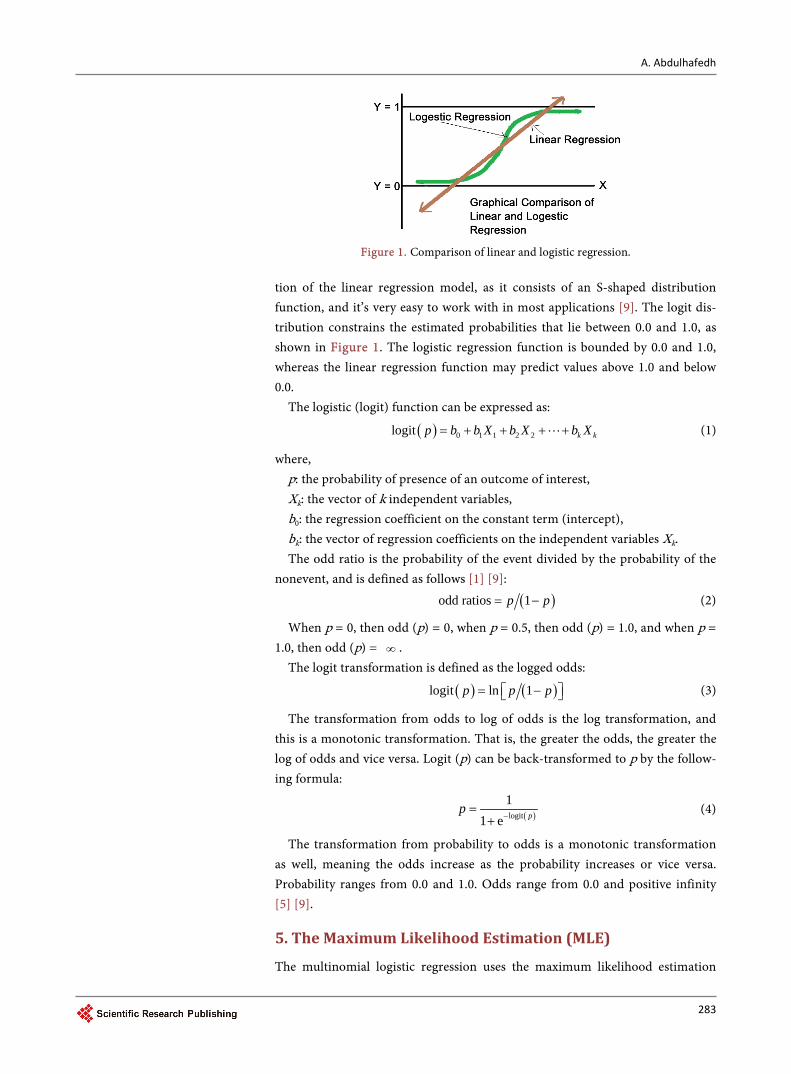
Figure 1. Comparison of linear and logistic regression.

tion of the linear regression model, as it consists of an S-shaped distribution function, and it’s very easy to work with in most applications [9]. The logit dis-tribution constrains the estimated probabilities that lie between 0.0 and 1.0, as shown in Figure 1. The logistic regression function is bounded by 0.0 and 1.0, whereas the linear regression function may predict values above 1.0 and below 0.0.

The logistic (logit) function can be expressed as:

( ) 0 1 1 2 2logit k kp b b X b X b X= + + + + (1)

where, p: the probability of presence of an outcome of interest, Xk: the vector of k independent variables, b0: the regression coefficient on the constant term (intercept), bk: the vector of regression coefficients on the independent variables Xk. The odd ratio is the probability of the event divided by the probability of the

nonevent, and is defined as follows [1] [9]:

( )odd ratios 1p p= − (2)

When p = 0, then odd (p) = 0, when p = 0.5, then odd (p) = 1.0, and when p = 1.0, then odd (p) = ∞ .

The logit transformation is defined as the logged odds:

( ) ( )logit ln 1p p p= − (3)

The transformation from odds to log of odds is the log transformation, and this is a monotonic transformation. That is, the greater the odds, the greater the log of odds and vice versa. Logit (p) can be back-transformed to p by the follow-ing formula:

( )logit

11 e p

p−+

= (4)

The transformation from probability to odds is a monotonic transformation as well, meaning the odds increase as the probability increases or vice versa. Probability ranges from 0.0 and 1.0. Odds range from 0.0 and positive infinity [5] [9].

5. The Maximum Likelihood Estimation (MLE)

The multinomial logistic regression uses the maximum likelihood estimation

A. Abdulhafedh

284

(MLE) to produce the regression parameters. Assuming that the random va-riables 1 2, , , nX X X form a random sample from a distribution ( )|f x θ ; if X is continuous random variable, ( )|f x θ is probability density function (pdf), if X is discrete random variable, ( )|f x θ is point mass function (pmf). The dis-tribution depends on a parameter θ, where θ could be a real unknown parameter or a vector of parameters. For every observed random sample 1, , nx x , we de-fine [10]:

( ) ( ) ( )1 1, , | | |n nf x x f x f xθ θ θ= (5)

If ( )|f x θ is pdf, ( )1, , |nf x x θ is the joint density function; if ( )|f x θ is pmf, ( )1, , |nf x x θ is the joint probability. The function ( )1, , |nf x x θ is the likelihood function, which depends on the unknown parameter θ, and it is denoted as L(θ). In order to get the maximum likelihood function, a value of θ for which the likelihood function L(θ) is a maximum is used as an estimate of θ. Maximizing L(θ) with a product of n terms is equivalent to maximizing logL(θ) because log is a monotonic increasing function. logL(θ) is a log likelihood func-tion, and is denoted as LL(θ), as follows [10]:

( ) ( ) ( ) ( )11log log | |nni iiiL f XL f Xθθ θ θ

=== == ∏ ∑ (6)

6. The Effect of Independent Variables

The effect of any independent variable on the outcome can be tested using the likelihood ratio (LR) statistic test. If the dependent variable has M categories, then there are M − 1 non redundant coefficients (βn) associated with each inde-pendent variable xn. The null hypothesis that xn does not affect the dependent variable can be written as:

0 ,1| , |: 0n Base n M BaseH β β= = = (7)

where Base is the base category used in the model. The hypothesis can be tested with the LR test. First, the LR estimates the full model that contains all of the in-dependent variables with the resulting LR statistic LRF. Second, the LR estimates the restricted model formed by excluding the independent variable xn with the resulting LR statistic LRR. Finally, the LR estimates the difference between LRF and LRR which is distributed as chi-square with n degrees of freedom (the num-ber of independent variables). The LR statistic is computed in terms of log like-lihood (LL) as follows [5] [10]:

( ) ( )2 of full model 2 of restricted modelLR LL LL= − − − (8)

F RLR LR LR= − (9)

Alternatively, the null model is given by (−2log(L0)) where L0 is the likelihood of obtaining the observations if the independent variables had no effect on the outcome (i.e. model with intercept alone). The full model is given by (−2log(L)) where L is the likelihood of obtaining the observations with all independent va-riables incorporated in the model. The difference of these two yields a Chi-Squared statistic which is a measure of how well the independent variables

A. Abdulhafedh

285

affect the outcome or dependent variable [1]. If the LR statistic for the overall model is significant, then there is evidence that the independent variables have contributed to the prediction of the outcome.

7. The Independence of Irrelevant Alternatives (IIA)

The MNL assumes that the odd ratios for any pair of outcomes (i.e. any pair of the dependent variable categories) are determined without reference to the other categories that might be available [2] [3]. This assumption is called the indepen-dence of irrelevant alternatives (IIA), which is very crucial in the MNL model-ing. If the IIA holds, then the MNL model can be used, if the IIA does not hold, then the MNL cannot be used and alternative models should be utilized such as, the nested MNL. The IIA can be tested by the Hausman specification test, pro-posed by Hausman and McFadden [11], which proceeds by estimating the error coefficients of the full model with all categories of the dependent variable in-cluded, then estimating the error coefficients of a restricted model by eliminat-ing one or more outcome categories. The null hypothesis of the test is that the IIA does not exist and estimators of the full and restricted models are consistent, and under the alternative hypothesis the IIA does exist and only the estimators of the restricted model are consistent. The test statistic HIIA is asymptotically distributed as chi square, and significant values of HIIA indicate that the IIA as-sumption is violated [11]. The Hausman specification test involves the following steps: 1) Estimate the error coefficients of the full model with all M categories of the

dependent variable included; these coefficients are contained in ˆfE .

2) Estimate the error coefficients of a restricted model by eliminating one or more outcome categories; theses coefficients are contained in ˆ

rE . 3) Let ˆ

fE∗ represents ˆfE after eliminating all coefficients not estimated in

the restricted model. The Hausman specification test of IIA is defined as [11]:

( ) ( ) ( ) ( )1ˆ ˆ ˆ ˆ ˆ ˆIIA r f r f r fH E E Var E Var E E E

−∗ ∗ ∗′ = − − − (10)

HIIA is asymptotically distributed as chi square with degrees of freedom equal to the rows in ˆ

rE . In this dissertation, the Hausman specification test will be applied on each outcome pair of the dependent variable (i.e. crash severity) sep-arately, excluding the other category of the dependent variable. Since the prop-erty damage is assumed to be the base category, as it is the most frequent oc-curred category, therefore the test will be applied on the minor injury vs. dis-abled injury first, and second; it will be applied on the minor injury vs. fatal in-jury, and lastly; it will be applied on the disabled injury vs. fatal injury. For each outcome pair, the test statistic HIIA will be obtained and compared to the full model with all outcomes. If the value of HIIA for any pair is significant, then the IIA assumption is violated and the MNL cannot be used in the modeling process. If the values of HIIA for all pairs are insignificant, then the IIA assump-tion holds and the MNL can be used in the modeling process.

A. Abdulhafedh

286

8. Multicollinearity

Multi-collinearity is the existence of linear relationships among the independent variables that can create inaccurate estimates of the regression coefficients, in-flate the standard errors of the regression coefficients, give false, non-significant p-values, and degrade the predictability of the model [1]. The source of the mul-ti-collinearity might come from data collection, sampling techniques, political or legal constraints, and outliers. Testing the multi-collinearity can be achieved by: (1) visual inspection of pairwise scatter plots of independent variables, and looking for near-perfect linear relationships between them; (2) Eigenvalues and Condition Indices; and (3) considering the variance inflation factors (VIF). The VIF is the most widely used test to measure how much the variance of the esti-mated regression coefficients are inflated as compared to when the predictor va-riables are not linearly related. The VIF may be calculated for each predictor by doing a linear regression of that predictor on all the other predictors, and then obtaining the R2 from that regression. The VIFs obtained by the linear regression can still be used in logistic regression models, because the concern is with the relationship among the independent variables included in the model, not with the functional form of the model [12]. Thus, a VIF of 1.6 tells us that the va-riance (the square of the standard error) of a particular coefficient is 60% larger than it would be if that predictor was completely uncorrelated with all other predictors. The VIF has a lower value of 1.0 but no upper bound. As a rule of thumb, if VIF is more than 10.0, then multicollinearity is considered a serious problem, and must be corrected [1] [12]. Variance inflation factors are scaled measures of the correlation coefficient between variable j and the rest of the in-dependent variables. Specifically:

2

11j

j

VIFR

=−

(11)

where, 2jR : is the coefficient of determination of the regression model that includes

all predictors except the jth predictor. Variance inflation factors are often given as the reciprocal of the above for-

mula. In this case, they are referred to as the tolerances. If 2jR equals zero (i.e.

no correlation between j and the remaining independent variables), then VIFj equals 1.0, and this is the minimum value.

9. The Generalized Hosmer-Lemeshow Statistic

The generalized Hosmer-Lemeshow test is used as an important goodness of fit measure to assess whether or not the observed events match expected events, by sub grouping the probabilities estimated from the data [13] [14]. The data set, of size n, is sorted according to the probabilities estimated from the final fitted MNL model. Then the data set is partitioned into several (Hosmer and Leme-show recommended 10) equal-sized groups. The first group corresponds to the n/10 observations having the highest estimated probabilities. The next group

A. Abdulhafedh

287

corresponds to the n/10 observations having the next highest estimated proba-bilities, etc. A Pearson-like chi square statistic is constructed based on the ob-served and expected group frequencies. In order to get the generalized test statis-tic (HL), we suppose that we have a sample of n independent observations, ( ), , 1, ,i ix y i n= . Recoding yi into binary indicator variables yij, such that yij = 1 when yi= j and yij= 0, otherwise ( 1, ,i n= and 0, , 1j c= − ). After fitting the model, let πij denote the estimated probabilities for each observation ( 1, ,i n= ) for each possible outcome ( 0, , 1j c= − ). By sorting the observations accord-ing to 1 − πi0, the complement of the estimated probability of the reference out-come. We then form g groups, each containing approximately n/g observations. For each group, we calculate the sums of the observed and estimated frequencies for each outcome category as follows [15]:

k ljlkj yO∈Ω

= ∑ (12)

k ljlkjE π∈Ω

= ∑ (13)

where Okj is the observed frequency, Ejk is the expected frequency, 1, ,k g= ; 0, , 1j c= − ; and Ωk denotes indices of the n/g observations in group k. The

multinomial goodness-of-fit (HL) test statistic is the Pearson’s chi-squared sta-tistic from the table of observed and estimated frequencies, and is given as [15]:

( )0

2

11

kj kjck

kj

gg j

O EC

E−

= ==

−∑ ∑ (14)

The distribution of Cg is chi-squared and has ( ) ( )2 1g c− × − degrees of freedom [16]. The null hypothesis is that the differences between the observed and predicted events are insignificant so the fitted model is correct, while the al-ternative hypothesis is that the differences are significant so the fitted model has deficiency and incorrect. If the test statistic HL is insignificant, then we will ac-cept the null hypothesis, and conclude that the fitted model is a good fit. If the test statistic HL is significant, then we will reject the null hypothesis, and con-clude that the data do not fit the hypothesized fitted MNL regression model.

10. The Classification Table of MNL

The classification table is another method to assess the goodness of fit of the MNL regression model. In this table the observed values for the dependent out-come and the predicted values (at a user defined cut-off value, for example p = 0.50) are cross-classified to indicate the correct % of predicted cases. This per-cent statistic assumes that if the estimated p is greater than or equal to 0.5 then the event is expected to occur and not occur otherwise. The bigger the % correct predictions, the better the model fit. We suppose for n observations that ( ),c j j′ is the ( ),j j th′ element of the classification table, , 1, ,j j J′ = . ( ),c j j′ is the sum of the frequencies for the observations whose actual re-

sponse category is j (as row) and predicted response category is j′ (as column) respectively. Then, the percentage of total correct predictions of the model is given by [4] [17]:

A. Abdulhafedh

288

( )1,

% total correct prediction 100%n

jjc j

n=

′∗=

∑ (15)

The percentage of correct predictions for response category j is given by:

( )

1

,% correct prediction of 100%m

iji

c j jj

n=

∗′

=∑

(16)

11. The Pseudo R-Squares

In ordinary least squared (OLS) regression there is a non-pseudo R-square, which is often generated as a goodness-of-fit measure, and is given by:

( )( )

22 1

2

1

ˆ1

ni ii

nii

y yR

y y=

=

−= −

−

∑∑

(17)

where n is the number of observations in the model, y is the dependent variable, y-bar is the mean of the y values, and y-hat is the value predicted by the model. The numerator of the ratio is the sum of the squared differences between the actual y values and the predicted y values. The denominator of the ratio is the sum of squared differences between the actual y values and their mean.

When analyzing data with a multinomial logistic regression, there is no an equivalent statistic to R-squared. The estimates from a logistic regression are found by the maximum likelihood estimation rather than the least squared esti-mation, so the OLS approach to goodness-of-fit does not apply. However, to evaluate the goodness-of-fit of logistic models, several pseudo R-squares have been developed. They are called “pseudo” R-squares because they are on a sim-ilar scale, ranging from 0 to 1 (though some pseudo R-squares never achieve 0 or 1) with higher values indicating better model fit, but they cannot be inter-preted as one would interpret an OLS R-squared, and different pseudo R- squares can present different values [12]. Some of the popular pseudo R-squares are:

McFadden’s R-square, which is defined as [18]:

2

0

ln1

lnM

McFLRL

= − (18)

where L0 is the value of the likelihood function for a model with no predictors (i.e. with intercept only), and LM is the likelihood function for the model being estimated. The ratio of the McFadden R-square indicates the level of improve-ment over the intercept model offered by the full model. Since a likelihood falls between 0.0 and 1.0, the log of a likelihood is less than or equal to zero. If a model has a very low likelihood, then the log of the likelihood will have a larger magnitude than the log of a more likely model. Thus, a small ratio of log like-lihoods indicates that the full model is a far better fit than the intercept model. When comparing two models on the same data, McFadden’s would be higher for the model with the greater likelihood. Another pseudo R-square is the Cox and Snell R2 which is defined as [19]:

A. Abdulhafedh

289

2 0&

2

1n

MC S

LL

R

= − (19)

where n is the sample size. The Cox and Snell R-square indicates the level of im-provement of the full model over the intercept model. This pseudo R-squared has a maximum value that is less than 1.0 when the full model predicts the out-come perfectly and has a likelihood of 1.0. The Nagelkerke R-square adjusts Cox & Snell’s so that the range of possible values extends to 1.0 by dividing by its maximum possible value, ( )2

01 nL− . If the full model perfectly predicts the outcome and has a likelihood of 1.0, then the Nagelkerke R-square = 1.0, which is defined as [20]:

( )

0

20

2

2

1

1

n

MnNK

LR

LL

−

−

= (20)

Pseudo R-squares are useful tools in evaluating multiple models predicting the same outcome on the same dataset, but they cannot be interpreted independent-ly or compared across different datasets. In other words, a pseudo R-squared statistic without context has little meaning. A pseudo R-squared only has mean-ing when compared to another pseudo R-squared of the same type, on the same data, predicting the same outcome [12] [21]. In this case, the higher pseudo R-squared indicates which model better predicts the outcome.

12. Estimation of Marginal Effects

Marginal effects are useful estimates of the impact of a one-unit change of an independent variable (predictor) on the dependent variable. The average mar-ginal effects are interpreted as the effect of a one-unit change in an independent variable (keeping all other independent variables constant at their mean values) on dependent variable. It is common to use a single average marginal effect val-ue for all observations of an independent variable. Elasticity analysis can also be used to interpret the effect of a specific independent variable on the dependent variable, but with a 1.0% change instead of a one-unit change. In MNL, the mar-ginal effect of an explanatory variable (predictor) is the partial derivative of the event probability with respect to the predictor of interest (i.e. the change in the event probability for a unit change in the predictor). The marginal effect for a dummy independent variable is the difference of the predicted probability values at their different levels [17]. The values of the marginal effects reflect the slopes of lines tangent to each of the predictors that is drawn tangent to the fitted probability curve at the selected point. The slope of the tangent line is the change in event probability, p, measured at two points, one unit apart along this straight line. If the probability curve is linear (near p = 0.5) at the selected point, then the marginal effect will approximate the probability change when changing the pre-dictor by one unit. If the probability curve is nonlinear (near the smallest and largest values of p), the marginal effect might deviate from the change [4] [17].

A. Abdulhafedh

290

For multinomial logistic regression models, the possible response values are un-ordered with levels 1, 2, ,i k= . The probability of response level i is given by [22]:

( )( )( )

ii

ij

EXP Xp

EXP Xββ

′=

′∑ (20)

where X ′ is the predictor of interest, and iβ is the regression coefficient (i.e. log odd) of X ′ . The marginal effect of the jth predictor, Xj, on pi is given by:

i i ki k

kj j j

p X Xp p

X X Xβ β ′ ′∂ ∂ ∂

= − ∂ ∂ ∂ ∑ (21)

13. Testing the Effects of Independent Variables

Multinomial logistic regression (MNL) is usually conducted using maximum li-kelihood estimation, which is an iterative procedure. The first iteration (called iteration zero) is the log likelihood of the null or empty model; that is, a model with no predictors. At the next iteration, the predictors are included in the mod-el. At each iteration, the log likelihood decreases as the goal is to minimize the log likelihood. When the difference between successive iterations is very small, the model is said to have converged, the iterating stops, and the final log likelih-ood (LR) statistic is computed. The log likelihood ration (LR) test statistic is ob-tained for the I-70 corridor for both the training and testing data, using the Stata 14 software package and reported in Table 1.

The effect of any independent variable on the outcome can be tested using the likelihood ratio (LR) statistic test. The null hypothesis of this test is that the in-dependent variables do not affect the dependent variable. The null model is cal-culated by obtaining the log likelihood of the observations with just the response variable in the model from iteration zero (i.e. model with intercept alone). The final fitted model is calculated by obtaining the log likelihood of observations with all the independent variables in the model from the final iteration after convergence. The difference of these two yields a chi-squared LR statistic which is a measure of how well the independent variables affect the outcomes or de-pendent variable categories [1]. If the LR statistic for the overall model is signif-icant, then there is evidence that the independent variables are effective and they have contributed to the prediction of the outcome. Table 1 shows that the Like-lihood Ratio (LR) test statistic for the I-70 corridor is significant at the 95% con-fidence level with p-values less than 0.05 for the training and testing datasets, implying that all the independent variables included in the models are not equal to zero, and this indicates that they are effectively contributing to modeling the

Table 1. The LR statistic results.

Dataset # Observations LR statistic p-value

I-70 Training data 4108 339.12 0.0000

I-70 Testing data 1761 122.44 0.0000

A. Abdulhafedh

291

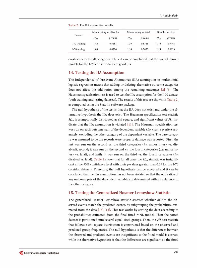
Table 2. The IIA assumption results.

Dataset Minor injury vs. disabled Minor injury vs. fatal Disabled vs. fatal

HIIA p-value HIIA p-value HIIA p-value

I-70 training 1.46 0.5461 1.39 0.6725 1.73 0.7748

I-70 testing 1.08 0.6726 1.14 0.7453 1.24 0.6833

crash severity for all categories. Thus, it can be concluded that the overall chosen models for the I-70 corridor data are good fits.

14. Testing the IIA Assumption

The Independence of Irrelevant Alternatives (IIA) assumption in multinomial logistic regression means that adding or deleting alternative outcome categories does not affect the odd ratios among the remaining outcomes [2] [3]. The Hausman specification test is used to test the IIA assumption for the I-70 dataset (both training and testing datasets). The results of this test are shown in Table 2, as computed using the Stata 14 software package.

The null hypothesis of the test is that the IIA does not exist and under the al-ternative hypothesis the IIA does exist. The Hausman specification test statistic HIIA is asymptotically distributed as chi square, and significant values of HIIA in-dicate that the IIA assumption is violated [11]. The Hausman specification test was run on each outcome pair of the dependent variable (i.e. crash severity) sep-arately, excluding the other category of the dependent variable. The base catego-ry was assumed to be the records were property damage was reported. First, the test was run on the second vs. the third categories (i.e. minor injury vs. dis-abled), second; it was run on the second vs. the fourth categories (i.e. minor in-jury vs. fatal), and lastly; it was run on the third vs. the fourth categories (i.e. disabled vs. fatal). Table 2 shows that for all cases the HIIA statistic was insignifi-cant at the 95% confidence level with their p-values greater than 0.05 for the I-70 corridor datasets. Therefore, the null hypothesis can be accepted and it can be concluded that the IIA assumption has not been violated so that the odd ratios of any outcome pair of the dependent variable are determined without reference to the other category.

15. Testing the Generalized Hosmer-Lemeshow Statistic

The generalized Hosmer-Lemeshow statistic assesses whether or not the ob-served events match the predicted events, by subgrouping the probabilities esti-mated from the data [13] [14]. This test works by sorting the data according to the probabilities estimated from the final fitted MNL model. Then the sorted dataset is partitioned into several equal-sized groups. Then, the HL test statistic that follows a chi-square distribution is constructed based on the observed and predicted group frequencies. The null hypothesis is that the differences between the observed and predicted events are insignificant so the fitted model is correct, while the alternative hypothesis is that the differences are significant so the fitted

A. Abdulhafedh

292

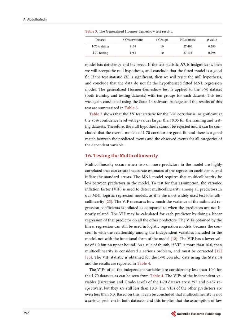
Table 3. The Generalized Hosmer-Lemeshow test results.

Dataset # Observations # Groups HL statistic p-value

I-70 training 4108 10 27.406 0.286

I-70 testing 1761 10 27.134 0.298

model has deficiency and incorrect. If the test statistic HL is insignificant, then we will accept the null hypothesis, and conclude that the fitted model is a good fit. If the test statistic HL is significant, then we will reject the null hypothesis, and conclude that the data do not fit the hypothesized fitted MNL regression model. The generalized Hosmer-Lemeshow test is applied to the I-70 dataset (both training and testing datasets) with ten groups for each dataset. This test was again conducted using the Stata 14 software package and the results of this test are summarized in Table 3.

Table 3 shows that the HL test statistic for the I-70 corridor is insignificant at the 95% confidence level with p-values larger than 0.05 for the training and test-ing datasets. Therefore, the null hypothesis cannot be rejected and it can be con-cluded that the overall models of I-70 corridor are good fit, and there is a good match between the predicted events and the observed events for all categories of the dependent variable.

16. Testing the Multicollinearity

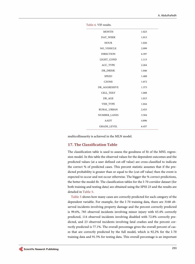
Multicollinearity occurs when two or more predictors in the model are highly correlated that can create inaccurate estimates of the regression coefficients, and inflate the standard errors. The MNL model requires that multicollinearity be low between predictors in the model. To test for this assumption, the variance inflation factor (VIF) is used to detect multicollinearity among all predictors in our MNL logistic regression models, as it is the most widely used test formulti-collinearity [23]. The VIF measures how much the variance of the estimated re-gression coefficients is inflated as compared to when the predictors are not li-nearly related. The VIF may be calculated for each predictor by doing a linear regression of that predictor on all the other predictors. The VIFs obtained by the linear regression can still be used in logistic regression models, because the con-cern is with the relationship among the independent variables included in the model, not with the functional form of the model [12]. The VIF has a lower val-ue of 1.0 but no upper bound. As a rule of thumb, if VIF is more than 10.0, then multicollinearity is considered a serious problem, and must be corrected [12] [23]. The VIF statistic is obtained for the I-70 corridor data using the Stata 14 and the results are reported in Table 4.

The VIFs of all the independent variables are considerably less than 10.0 for the I-70 datasets as can be seen from Table 4. The VIFs of the independent va-riables (Direction and Grade-Level) of the I-70 dataset are 6.397 and 6.457 re-spectively, but they are still less than 10.0. The VIFs of the other predictors are even less than 5.0. Based on this, it can be concluded that multicollinearity is not a serious problem in both datasets, and this implies that the assumption of low

A. Abdulhafedh

293

Table 4. VIF results.

MONTH 1.023

DAY_WEEK 1.013

HOUR 1.026

NO_VEHICLE 2.099

DIRECTION 6.397

LIGHT_COND 1.113

ACC_TYPE 2.264

DR_DRINK 1.046

SPEED 1.408

CZONE 1.072

DR_AGGRESSIVE 1.373

CELL_TEXT 1.008

DR_AGE 1.015

VEH_TYPE 1.044

RURAL_URBAN 2.455

NUMBER_LANES 3.504

AADT 4.896

GRADE_LEVEL 6.457

multicollinearity is achieved in the MLN model.

17. The Classification Table

The classification table is used to assess the goodness of fit of the MNL regres-sion model. In this table the observed values for the dependent outcomes and the predicted values (at a user defined cut-off value) are cross-classified to indicate the correct % of predicted cases. This percent statistic assumes that if the pre-dicted probability is greater than or equal to the (cut-off value) then the event is expected to occur and not occur otherwise. The bigger the % correct predictions, the better the model fit. The classification tables for the I-70 corridor dataset (for both training and testing data) are obtained using the SPSS 23 and the results are detailed in Table 5.

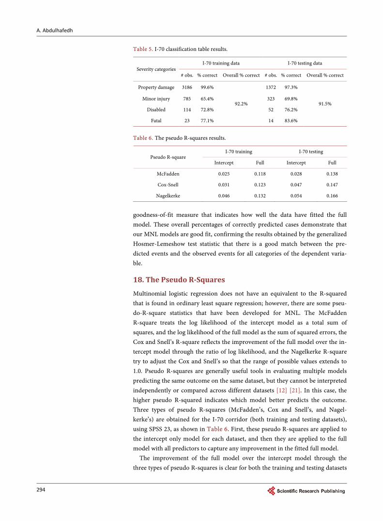
Table 5 shows how many cases are correctly predicted for each category of the dependent variable. For example, for the I-70 training data, there are 3168 ob-served incidents involving property damage and the percent correctly predicted is 99.6%, 785 observed incidents involving minor injury with 65.4% correctly predicted, 114 observed incidents involving disabled with 72.8% correctly pre-dicted, and 23 observed incidents involving fatal crashes and the percent cor-rectly predicted is 77.1%. The overall percentage gives the overall percent of cas-es that are correctly predicted by the full model, which is 92.2% for the I-70 training data and 91.5% for testing data. This overall percentage is an important

A. Abdulhafedh

294

Table 5. I-70 classification table results.

Severity categories I-70 training data I-70 testing data

# obs. % correct Overall % correct # obs. % correct Overall % correct

Property damage 3186 99.6%

92.2%

1372 97.3%

91.5% Minor injury 785 65.4% 323 69.8%

Disabled 114 72.8% 52 76.2%

Fatal 23 77.1% 14 83.6%

Table 6. The pseudo R-squares results.

Pseudo R-square I-70 training I-70 testing

Intercept Full Intercept Full

McFadden 0.025 0.118 0.028 0.138

Cox-Snell 0.031 0.123 0.047 0.147

Nagelkerke 0.046 0.132 0.054 0.166

goodness-of-fit measure that indicates how well the data have fitted the full model. These overall percentages of correctly predicted cases demonstrate that our MNL models are good fit, confirming the results obtained by the generalized Hosmer-Lemeshow test statistic that there is a good match between the pre-dicted events and the observed events for all categories of the dependent varia-ble.

18. The Pseudo R-Squares

Multinomial logistic regression does not have an equivalent to the R-squared that is found in ordinary least square regression; however, there are some pseu-do-R-square statistics that have been developed for MNL. The McFadden R-square treats the log likelihood of the intercept model as a total sum of squares, and the log likelihood of the full model as the sum of squared errors, the Cox and Snell’s R-square reflects the improvement of the full model over the in-tercept model through the ratio of log likelihood, and the Nagelkerke R-square try to adjust the Cox and Snell’s so that the range of possible values extends to 1.0. Pseudo R-squares are generally useful tools in evaluating multiple models predicting the same outcome on the same dataset, but they cannot be interpreted independently or compared across different datasets [12] [21]. In this case, the higher pseudo R-squared indicates which model better predicts the outcome. Three types of pseudo R-squares (McFadden’s, Cox and Snell’s, and Nagel-kerke’s) are obtained for the I-70 corridor (both training and testing datasets), using SPSS 23, as shown in Table 6. First, these pseudo R-squares are applied to the intercept only model for each dataset, and then they are applied to the full model with all predictors to capture any improvement in the fitted full model.

The improvement of the full model over the intercept model through the three types of pseudo R-squares is clear for both the training and testing datasets

A. Abdulhafedh

295

of I-70. For example, the McFadden R-square value for the I-70 training dataset is increased from 0.025 for the intercept to 0.118 for the full model, the Cox and Snell R-square value is increased from 0.031 for the intercept to 0.123 for the full model, and the Nagelkerke R-square is also increased from 0.046 for the inter-cept to 0.132 for the full mode. The higher pseudo R-squared values for the full models compared to the intercept models indicate that the fitted full models better predict the outcomes of the dependent variable, and the predictors are ef-fective in modeling the different outcomes of the crash severity.

19. Results of Multinomial Logistic Regression

The prediction results of the MNL are shown in the following sections:

19.1. Predicted Odd Ratios for I-70 Corridor

The odd ratios in MNL models present the probability of the event divided by the probability of the nonevent, and they can be obtained by exponentiating the multinomial logit coefficients (i.e. e(coef.)). The multinomial logistic regression model estimates (k − 1) models, where k is the number of outcome levels of the dependent variable, and the kth equation is relative to the referent group. In our model, the property damage is considered as the referent group (i.e. base level), because it is the most frequent outcome of crash severity, and the other outcome levels (i.e. minor injury, disabled, and fatal) are estimated relative to the property damage. The standard interpretation of the multinomial logistic regression is that for a unit change in the predictor variable, the odd ratio of outcome m rela-tive to the referent group is expected to change by its respective parameter esti-mate given the other predictors in the model are held constant [1] [9]. The pre-dicted odd ratios for the I-70 corridor (for both training and testing data) are obtained using Stata 14 and reported in Table 7. The odd ratios are significant when their related p-values at the 95% confidence level are less than 0.05. If the odd ratios are greater than 1.0, then the predictors are positively correlated with the dependent variable (i.e. crash severity), and if the odd ratios are smaller than 1.0, then the predictors are negatively correlated with the dependent variable. In other words, if the odd ratios are greater than 1.0, then the predictors would in-crease the likelihood of the crash severity occurrence at the specified level, indi-cating positive contribution to the crash severity occurrence at that level, and if the odd ratios are smaller than 1.0, then the predictors would decrease the like-lihood of the crash severity occurrence at the specified level, indicating negative contribution to the crash occurrence at that level.

For example, when inspecting the MONTH predictor in the 1st case of crash severity (i.e. minor injury relative to property damage) in Table 7 for the train-ing dataset, the odd ratio is greater than 1.0 (i.e. 1.015594), which indicates that this predictor is positively contributing to the crash severity at this level (i.e. minor injury), however, it is not significant at the 95% confidence as its p-value is greater than 0.05. In other words, the contribution of the predictor MONTH to the crash severity of the level of minor injury, would be expected to increase

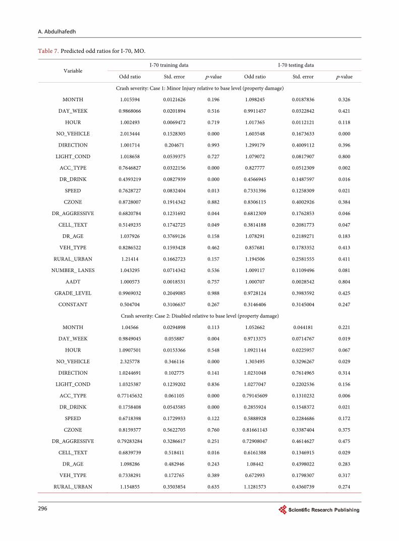
A. Abdulhafedh

296

Table 7. Predicted odd ratios for I-70, MO.

Variable I-70 training data I-70 testing data

Odd ratio Std. error p-value Odd ratio Std. error p-value

Crash severity: Case 1: Minor Injury relative to base level (property damage)

MONTH 1.015594 0.0121626 0.196 1.098245 0.0187836 0.326

DAY_WEEK 0.9868066 0.0201894 0.516 0.9911457 0.0322842 0.421

HOUR 1.002493 0.0069472 0.719 1.017365 0.0112121 0.118

NO_VEHICLE 2.013444 0.1528305 0.000 1.603548 0.1673633 0.000

DIRECTION 1.001714 0.204671 0.993 1.299179 0.4009112 0.396

LIGHT_COND 1.018658 0.0539375 0.727 1.079072 0.0817907 0.800

ACC_TYPE 0.7646827 0.0322156 0.000 0.827777 0.0512309 0.002

DR_DRINK 0.4393219 0.0827939 0.000 0.4566945 0.1487597 0.016

SPEED 0.7628727 0.0832404 0.013 0.7331396 0.1258309 0.021

CZONE 0.8728007 0.1914342 0.882 0.8306115 0.4002926 0.384

DR_AGGRESSIVE 0.6820784 0.1231692 0.044 0.6812309 0.1762853 0.046

CELL_TEXT 0.5149235 0.1742725 0.049 0.3814188 0.2081773 0.047

DR_AGE 1.037926 0.3769126 0.158 1.078291 0.2189271 0.183

VEH_TYPE 0.8286522 0.1593428 0.462 0.857681 0.1783352 0.413

RURAL_URBAN 1.21414 0.1662723 0.157 1.194506 0.2581555 0.411

NUMBER_ LANES 1.043295 0.0714342 0.536 1.009117 0.1109496 0.081

AADT 1.000573 0.0018531 0.757 1.000707 0.0028542 0.804

GRADE_LEVEL 0.9969032 0.2049085 0.988 0.9728124 0.3983592 0.425

CONSTANT 0.504704 0.3106637 0.267 0.3146406 0.3145004 0.247

Crash severity: Case 2: Disabled relative to base level (property damage)

MONTH 1.04566 0.0294898 0.113 1.052662 0.044181 0.221

DAY_WEEK 0.9849045 0.055887 0.004 0.9713375 0.0714767 0.019

HOUR 1.0907501 0.0153366 0.548 1.0921144 0.0225957 0.067

NO_VEHICLE 2.325778 0.346116 0.000 1.303495 0.3296267 0.029

DIRECTION 1.0244691 0.102775 0.141 1.0231048 0.7614965 0.314

LIGHT_COND 1.0325387 0.1239202 0.836 1.0277047 0.2202536 0.156

ACC_TYPE 0.77145632 0.061105 0.000 0.79145609 0.1310232 0.006

DR_DRINK 0.1758408 0.0543585 0.000 0.2855924 0.1548372 0.021

SPEED 0.6718398 0.1729933 0.122 0.5888928 0.2284686 0.172

CZONE 0.8159377 0.5622705 0.760 0.81661143 0.3387404 0.375

DR_AGGRESSIVE 0.79283284 0.3286617 0.251 0.72908047 0.4614627 0.475

CELL_TEXT 0.6839739 0.518411 0.016 0.6161388 0.1346915 0.029

DR_AGE 1.098286 0.482946 0.243 1.08442 0.4398022 0.283

VEH_TYPE 0.7338291 0.172765 0.389 0.672993 0.1798307 0.317

RURAL_URBAN 1.154855 0.3503854 0.635 1.1281573 0.4360739 0.274

A. Abdulhafedh

297

Continued

NUMBER_ LANES 1.0623837 0.1297353 0.035 1.0729747 0.327797 0.041

AADT 1.0900496 0.0048217 0.302 1.0993353 0.0064666 0.306

GRADE_LEVEL 0.99225575 0.095807 0.000 0.92474128 1.210746 0.015

CONSTANT 0.4430657 5.736671 0.273 0.42062742 0.40145 0.417

Crash severity: Case 3: Fatal relative to base level (property damage)

MONTH 1.204367 0.0806321 0.005 1.204406 0.0831499 0.014

DAY_WEEK 0.9863804 0.105922 0.737 0.9828217 0.1155401 0.177

HOUR 1.023859 0.0319797 0.450 1.036516 0.0377693 0.365

NO_VEHICLE 2.232134 0.5612323 0.001 1.707896 0.4912682 0.009

DIRECTION 1.099131 1.869167 0.515 1.042631 1.473025 0.231

LIGHT_COND 1.042018 0.6304126 0.001 1.038765 0.766612 0.007

ACC_TYPE 0.7563569 0.3752455 0.063 0.6287748 0.3629575 0.370

DR_DRINK 0.1747316 0.1104344 0.006 0.2648509 0.4530978 0.033

SPEED 0.3108948 0.2162619 0.093 0.3551321 0.334089 0.271

CZONE 0.82678563 0.1350873 0.081 0.8429472 0.244088 0.291

DR_AGGRESSIVE 0.8619844 3.320254 0.003 0.8827105 3.191887 0.008

CELL_TEXT 0.2562309 0.2849574 0.021 0.0714367 0.0850799 0.027

DR_AGE 1.0981655 0.7690331 0.295 1.0616548 0.2628931 0.319

VEH_TYPE 0.7822954 0.1692881 0.284 0.781194 0.1672393 0.342

RURAL_URBAN 1.3862095 0.4994118 0.605 1.4874849 0.4314113 0.217

NUMBER_ LANES 1.0718678 0.3198925 0.404 1.0565231 0.9127193 0.344

AADT 1.002445 0.0111129 0.226 1.0876658 0.0134131 0.361

GRADE_LEVEL 0.75853 0.7540079 0.781 0.82517107 2.630318 0.377

CONSTANT 0.68610 2.9507 0.916 0.677015 1.40901 0.487

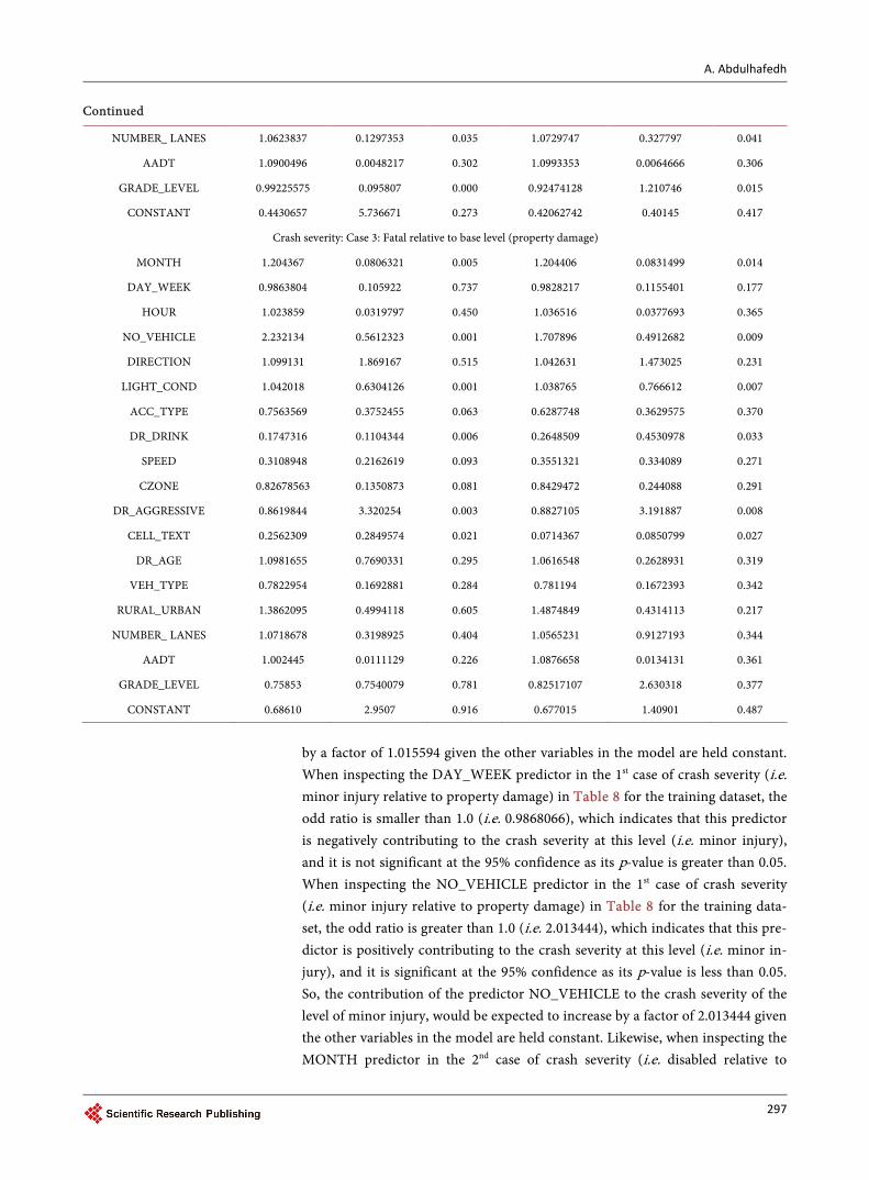
by a factor of 1.015594 given the other variables in the model are held constant. When inspecting the DAY_WEEK predictor in the 1st case of crash severity (i.e. minor injury relative to property damage) in Table 8 for the training dataset, the odd ratio is smaller than 1.0 (i.e. 0.9868066), which indicates that this predictor is negatively contributing to the crash severity at this level (i.e. minor injury), and it is not significant at the 95% confidence as its p-value is greater than 0.05. When inspecting the NO_VEHICLE predictor in the 1st case of crash severity (i.e. minor injury relative to property damage) in Table 8 for the training data-set, the odd ratio is greater than 1.0 (i.e. 2.013444), which indicates that this pre-dictor is positively contributing to the crash severity at this level (i.e. minor in-jury), and it is significant at the 95% confidence as its p-value is less than 0.05. So, the contribution of the predictor NO_VEHICLE to the crash severity of the level of minor injury, would be expected to increase by a factor of 2.013444 given the other variables in the model are held constant. Likewise, when inspecting the MONTH predictor in the 2nd case of crash severity (i.e. disabled relative to

A. Abdulhafedh

298

Table 8. Significant risk factors for I-70, MO.

Crash severity level INTERSTATE I-70, MO

Significant risk factors Significant group factors

Case 1: minor injury

1. NO_VEHICLE

2. ACC_TYPE

3. DR_DRINK

4. SPEED

5. DR_AGGRESSIVE

6. CELL_TEXT

1. Driver behavior

2. Accident type

Case 2: disabled

1. DAY_WEEK

2. NO_VEHICLE

3. ACC_TYPE

4. DR_DRINK

5. CELL_TEXT

6. NUMBER_LANES

7. GRADE_LEVEL

1. Time

2. Driver Behavior

3. Accident type

4. Road geometry

Case 3: fatal

1. MONTH

2. NO_VEHICLES

3. LIGHT_COND

4. DR_DRINK

5. DR_AGGRESSIVE

6. CELL_TEXT

1. Time

2. Driver behavior

3. Environment

property damage) in Table 7 for the training dataset, the odd ratio is greater than 1.0 (i.e. 1.04566), which indicates that this predictor is positively contri-buting to the crash severity at this level (i.e. disabled), however it is not signifi-cant at the 95% confidence as its p-value is greater than 0.05. In other words, the contribution of the predictor MONTH to the crash severity of the level of “dis-abled”, would be expected to increase by a factor of 1.04566 given the other va-riables in the model are held constant. When inspecting the MONTH predictor in the 3rd case of crash severity (i.e. fatal relative to property damage) in Table 8 for the training dataset, the odd ratio is greater than 1.0 (i.e. 1.204367), which indicates that this predictor is positively contributing to the crash severity at this level (i.e. fatal), and it is significant at the 95% confidence as its p-value is less than 0.05. When inspecting the NO_VEHICLE predictor in the 2nd and 3rd cases of crash severity (i.e. disabled relative to property damage, and fatal relative to property damage) in Table 7 for the training dataset, the odd ratios are greater than 1.0 (i.e. 2.325778, 2.232134 respectively), which indicates that this predictor is positively contributing to the crash severity at these two levels (i.e. disabled, and fatal), and it is significant at the 95% confidence as its p-values are less than 0.05. So, the contribution of the predictor NO_VEHICLE to the crash severity of the levels of “disabled” and “fatal”, would be expected to increase by a factor of 2.325778 and 2.232134 respectively given the other variables in the model are held constant.

A. Abdulhafedh

299

19.2. Significant Risk Factors for I-70 Corridor

The statistically significant risk factors (i.e. predictors or independent variables) of the I-70 corridor in Missouri at the 95% confidence level are shown in Table 8.

For the 1st case of crash severity level (i.e. minor injury relative to property damage), the number of vehicles involved in the crashes, the accident type, the driver drink, the speed, the driver aggressiveness, and the cell-text, are signifi-cant at the 95% confidence level. For the 2nd case of crash severity level (i.e. dis-abled relative to property damage), the day of the week, the number of vehicles involved in the crashes, the accident type, the driver drink, the cell-text, the number of lanes, and the grade of the road are significant at the 95% confidence level. For the 3rd case of crash severity level (i.e. fatal relative to property dam-age), the month of the year, the number of vehicles involved in the crashes, the light condition, the driver drink, the driver aggressiveness, and the cell-text, are significant at the 95% confidence level. We can see that two risk factors (i.e. the number of vehicles involved in the crashes and using the cell phones or texts when driving) are significant at the three crash severity levels (i.e. minor injury, disabled, fatal), indicating the importance of these two risk factors in modeling the severity of crashes of the I-70 corridor in MO. Some other risk factors are significant at only two levels of crash severity, but not at the third level. These risk factors are the accident type, the driver drink, and the driver aggressiveness. The speed, the light condition, the number of lanes, the grade of the road, the day of the week, and the month of the year are significant at only one level of crash severity. In term of the significant group of factors, we can see that the driver’s behavior group is the most important one as it has been related to the three crash severity levels, whereas the accident type, the time, is the next in its importance.

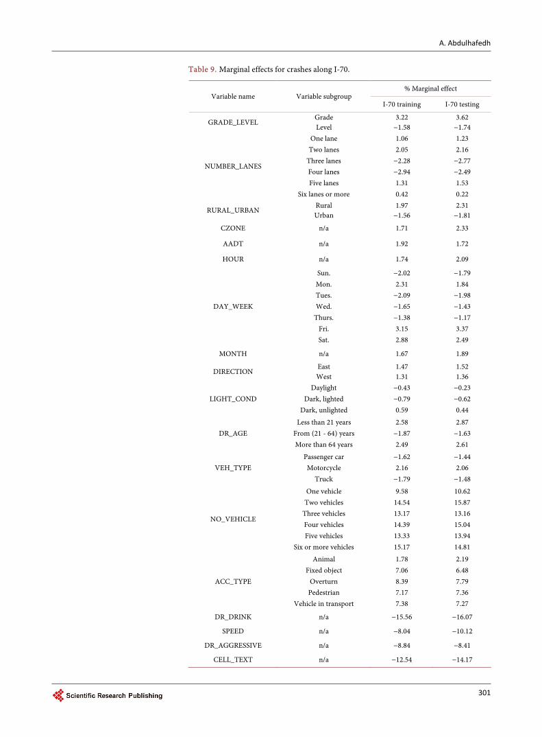
19.3. Marginal Effects for Crashes along I-70 Corridor

The marginal effect reflects the impact of a one-unit change of an independent variable (predictor) on the event probability of the dependent variable (keeping all other independent variables constant at their mean values). In MNL, the marginal effect of an explanatory variable (predictor) is the partial derivative of the event probability with respect to the predictor of interest (i.e. the change in the event probability of the dependent variable for a unit change in the predic-tor), and they could be positive or negative values. Positive values indicate that the predictor would positively contribute to crash severity (i.e. would increase the degree severity of crashes), and negative values indicate that the predictor would negatively contribute to crash severity (i.e. would decrease the degree se-verity of crashes). The marginal effect for a dummy or discrete independent va-riable is the difference of the predicted probability values at their different levels [17]. The marginal effects for the I-70 corridor (for both training and testing da-ta) are obtained using Stata 14 and reported in Table 9. It can be seen from the table that some predictors have higher marginal effects than others. For instance,

A. Abdulhafedh

300

the driver drink predictor has a marginal effect of 15.56% for training data, and 16.07% for testing data. These values present the difference of the event proba-bility of the crash severity when drivers using the road being drunk and not drunk.

In other words, if all the drivers that use the I-70 corridor in MO were not in intoxicated conditions, then the probability of crash severity at the I-70 corridor would decrease by 15.56% using training data and 16.07% using testing data. The speed predictor has a marginal effect of 8.04 % for training data, and 10.12% for testing data. These values present the difference of the event probability of the crash severity when drivers using the road are speeding and not speeding so that the crash severity would decrease by (8.04% using training data and 10.12% using testing data) if all drivers were not speeding. The cell-text predictor has a marginal effect of 12.54% for training data, and 14.17% for testing data. These values present the difference of the event probability of the crash severity when drivers are using the cell phones and/or texting during the driving and not using them so that the crash severity would decrease by 12.54% using training data and 14.17% using testing data if all drivers were not using cell-text when driving. The number of vehicles involved (assuming one vehicle) in the crash has a marginal effect of 9.58% for training data, and 10.62% for testing data. Meaning that if only one vehicle is involved in the crash, then it would increase the severity by 9.58% using training data and 10.62% using testing data. However, if the number of vehicles involved were increased to two vehicles, then this would increase the severity by 14.54% using training data and 15.87% using testing data. If the number of vehicles increased to three vehicles, then this would increase the se-verity by 13.17% using training data and 13.16% using testing data. If the num-ber of vehicles further increased to four vehicles, then this would increase the severity by 14.39% using training data and 15.04% using testing data. The acci-dent type predictor (ACC_TYPE) relative to an animal has a marginal effect of 1.78% for training data and 2.19% for testing data. Meaning if an animal would have caused the accident, then this would increase the severity by 1.78% using training data and 2.19% using testing data. However, the accident type predictor relative to a fixed object has a marginal effect of 7.06% for training data and 6.48% for testing data. Meaning if a fixed object (such as a tree or a traffic sign) would have caused the accident, then this would increase the severity by 7.06% using training data and 6.48% using testing data. However, the accident type predictor relative to an overturn has a marginal effect of 8.39% for training data and 7.79% for testing data. Meaning if an overturn was the accident type, then this would increase the severity by 8.39% using training data and 7.79% using testing data. Similarly, the accident type predictor relative to a pedestrian has a marginal effect of 7.17% for training data and 7.36% for testing data. Meaning if a pedestrian would have caused the accident, then this would increase the sever-ity by 7.17% using training data and 7.36% using testing data. In similar manner, the accident type predictor relative to a vehicle in transport has a marginal effect of 7.38% for training data and 7.27% for testing data. Meaning if a vehicle in

A. Abdulhafedh

301

Table 9. Marginal effects for crashes along I-70.

Variable name Variable subgroup % Marginal effect

I-70 training I-70 testing

GRADE_LEVEL Grade Level

3.22 −1.58

3.62 −1.74

NUMBER_LANES

One lane Two lanes

Three lanes Four lanes Five lanes

Six lanes or more

1.06 2.05

−2.28 −2.94 1.31 0.42

1.23 2.16

−2.77 −2.49 1.53 0.22

RURAL_URBAN Rural Urban

1.97 −1.56

2.31 −1.81

CZONE n/a 1.71 2.33

AADT n/a 1.92 1.72

HOUR n/a 1.74 2.09

DAY_WEEK

Sun. Mon. Tues. Wed.

Thurs. Fri. Sat.

−2.02 2.31

−2.09 −1.65 −1.38 3.15 2.88

−1.79 1.84

−1.98 −1.43 −1.17 3.37 2.49

MONTH n/a 1.67 1.89

DIRECTION East West

1.47 1.31

1.52 1.36

LIGHT_COND Daylight

Dark, lighted Dark, unlighted

−0.43 −0.79 0.59

−0.23 −0.62 0.44

DR_AGE Less than 21 years

From (21 - 64) years More than 64 years

2.58 −1.87 2.49

2.87 −1.63 2.61

VEH_TYPE Passenger car Motorcycle

Truck

−1.62 2.16

−1.79

−1.44 2.06

−1.48

NO_VEHICLE

One vehicle Two vehicles

Three vehicles Four vehicles Five vehicles

Six or more vehicles

9.58 14.54 13.17 14.39 13.33 15.17

10.62 15.87 13.16 15.04 13.94 14.81

ACC_TYPE

Animal Fixed object

Overturn Pedestrian

Vehicle in transport

1.78 7.06 8.39 7.17 7.38

2.19 6.48 7.79 7.36 7.27

DR_DRINK n/a −15.56 −16.07

SPEED n/a −8.04 −10.12

DR_AGGRESSIVE n/a −8.84 −8.41

CELL_TEXT n/a −12.54 −14.17

A. Abdulhafedh

302

transport would have caused the accident, then this would increase the severity by 7.38% using training data and 7.27% using testing data.

20. Conclusion

This paper applied multinomial logistic regression (MNL) to model the rela-tionships of the crash severity categories with the independent variables. The I-70 corridor is tested under the assumptions of the MNL. The categories of the dependent variable (i.e. fatal, disabling injury, minor injury, property-damage- only) are considered nominal (i.e. cannot be ordered in any logical way). This paper investigated the use of a wider range of independent variables (i.e. risk factors) in crash severity modeling, given that past research has only made use of limited numbers/types of independent variables. In addition, this paper intro-duced a variety of new procedures in presenting the results of the MNL applica-tions that have not been reported in other crash severity models, including: 1) the use of the odd ratios as regression estimates instead of using regression coef-ficients to interpret the results of prediction; 2) a focus on the assumption of the independence of irrelevant alternatives (IIA) that is very important in the MNL modeling, using the Hausman specification test; 3) consideration of the genera-lized Hosmer-Lemeshow test as an important goodness of fit measure to assess whether or not the observed incidents match the predicted incidents; 4) the use of the classification table as a measure of goodness of fit to determine the per-cent of corrected prediction cases; 5) testing for the multicollinearity among the independent variables as precondition assumption; 6) the use of the pseudo R squares as potential goodness of fits instead of classical measures of goodness of fit, such as the Deviance, the Akaike Information Criteria (AIC), and the Baye-sian Information Criteria (BIC); and 7) presenting the marginal effects of all in-dependent variables upon the dependent variable. Results showed the effective-ness of the MNL approach in crash severity modeling.

References [1] Greene, W. (2012) Econometric Analysis. 7th Edition, Prentice Hall, Upper Saddle

River.

[2] McFadden, D., Tye, W. and Train, K. (1976) An Application of Diagnostic Tests for the Independence from Irrelevant Alternatives Property of the Multinomial Logit Model. Transportation Research Record, 637, 39-45.

[3] Hausman, J.A. (1978) Specification Tests in Econometrics. Econometrica, 46, 1251- 1271. https://doi.org/10.2307/1913827

[4] Kleinbaum, D.G. and Klein, M. (2010) Logistic Regression: A Self-Learning Text. 3rd Edition, Springer, New York. https://doi.org/10.1007/978-1-4419-1742-3

[5] Baltagi, B.H. (2011) Econometrics. 5th Edition, Springer, Berlin. https://doi.org/10.1007/978-3-642-20059-5

[6] Abdel-Aty, M. (2003) Analysis of Driver Injury Severity Levels at Multiple Loca-tions Using Ordered Probit Models. Journal of Safety Research, 34, 597-603. https://doi.org/10.1016/j.jsr.2003.05.009

[7] Bham, G., Javvadi, B. and Manepalli, U. (2012) Multinomial Logistic Regression

A. Abdulhafedh

303

Model for Single-Vehicle and Multivehicle Collisions on Urban U.S. Highways in Arkansas. Journal of Transportation Engineering, 138, 786-797. https://doi.org/10.1061/(ASCE)TE.1943-5436.0000370

[8] The Missouri State Highway Patrol (2016) Accident Investigation Reports. https://www.mshp.dps.missouri.gov/HP68/static/Official.html

[9] Judge, G., Griffiths, W.E., Hill, R.C., Lutkepohl, H. and Lee, T.C. (1985) The Theory and Practice of Econometrics. 2nd Edition, Wiley, New York.

[10] Long, S. (1996) Regression Models for Categorical and Limited Dependent Va-riables. Sage Publications, Thousand Oaks.

[11] Hausman, J.A. and McFadden, D. (1984) Specification Tests for the Multinomial Logit Model. Econometrica, 52, 1219-1240. https://doi.org/10.2307/1910997

[12] Menard, S. (2002) Applied Logistic Regression Analysis. Sage Publications, Thou-sand Oaks.

[13] Lemeshow, S.A. and Hosmer, J.D.W. (1982) A Review of Goodness of Fit Statistics for the Use in the Development of Logistic Regression Models. American Journal of Epidemiology, 115, 92-106. https://doi.org/10.1093/oxfordjournals.aje.a113284

[14] Hosmer, D.W., Lemeshow, S.A. and Sturdivant, R.X. (2013) Applied Logistic Regre- ssion. 3rd Edition, Wiley, Hoboken. https://doi.org/10.1002/9781118548387

[15] Fagerland, M.W. and Hosmer, D.W.J. (2012) A Generalized Hosmer Leme Show Goodness-of-Fit Test for Multinomial Logistic Regression Models. Stata Journal, 12, 447-453.

[16] Fagerland, M.W., Hosmer, D.W. and Bofin, A.M. (2008) Multinomial Goodness-of- Fit Tests for Logistic Regression Models. Statistics in Medicine, 27, 4238-4253. https://doi.org/10.1002/sim.3202

[17] Long, S. and Freese, J. (2014) Regression Models for Categorical Dependent Va-riables Using Stata. 3rd Edition, Stata Press, College Station.

[18] McFadden, D. (1974) Conditional Logit Analysis of Qualitative Choice Behavior. Frontiers in Econometrics, 105-142.

[19] Cox, D.R. and Snell, E.J. (1989) Analysis of Binary Data. 2nd Edition, Chapman & Hall, London.

[20] Nagelkerke, N.J.D. (1991) A Note on a General Definition of the Coefficient of De-termination. Biometrika, 78, 691-692. https://doi.org/10.1093/biomet/78.3.691

[21] Tjur, T. (2009) Coefficients of Determination in Logistic Regression Models: A New Proposal: The Coefficient of Discrimination. The American Statistician, 63, 366- 372. https://doi.org/10.1198/tast.2009.08210

[22] Freese, J. and Long, J.S. (2000) Tests for the Multinomial Logit Model. Stata Techni- cal Bulletin, 10, 247-255.

[23] Greene, W. (2008) Econometric Analysis. 6th Edition, Prentice-Hall, Upper Saddle River.

Submit or recommend next manuscript to SCIRP and we will provide best service for you:

Accepting pre-submission inquiries through Email, Facebook, LinkedIn, Twitter, etc. A wide selection of journals (inclusive of 9 subjects, more than 200 journals) Providing 24-hour high-quality service User-friendly online submission system Fair and swift peer-review system Efficient typesetting and proofreading procedure Display of the result of downloads and visits, as well as the number of cited articles Maximum dissemination of your research work

Submit your manuscript at: http://papersubmission.scirp.org/ Or contact jtts@scirp.org