INDEBTED DEMAND*

ATIF MIANLUDWIG STRAUB

AMIR SUFI

February 11, 2021

Abstract

We propose a theory of indebted demand, capturing the idea that large debt burdens loweraggregate demand, and thus the natural rate of interest. At the core of the theory is the simpleyet under-appreciated observation that borrowers and savers differ in their marginal propen-sities to save out of permanent income. Embedding this insight in a two-agent perpetual-youth model, we find that recent trends in income inequality and financial deregulation leadto indebted household demand, pushing down the natural rate of interest. Moreover, popu-lar expansionary policies—such as accommodative monetary policy—generate a debt-financedshort-run boom at the expense of indebted demand in the future. When demand is sufficientlyindebted, the economy gets stuck in a debt-driven liquidity trap, or debt trap. Escaping a debttrap requires consideration of less conventional macroeconomic policies, such as those focusedon redistribution or those reducing the structural sources of high inequality. JEL Codes: E21,E43, G51, E52, E62.

*We are very grateful to the editor and four anonymous referees, who helped significantly improve the paper.We also thank George-Marios Angeletos, Heather Boushey, Francois Gourio, Fatih Guvenen, Gerhard Illing, ErnestLiu, Fabrizio Perri, Alp Simsek, Jeremy Stein, Larry Summers, and Ivan Werning as well as engaged seminar par-ticipants at several institutions for numerous useful comments. Jan Ertl, Sophia Mo, and Ian Sapollnik provided ex-cellent research assistance. Straub appreciates support from the Molly and Domenic Ferrante Award. Contact info:Mian: (609) 258 6718, atif@princeton.edu; Straub: (617) 496 9188, ludwigstraub@fas.harvard.edu; Sufi: (773) 702 6148,amir.sufi@chicagobooth.edu

1

I Introduction

Rising debt and falling rates of return have characterized advanced economies over the past 40years. As shown in Figure 1, debt owed by households and the government in the United Stateshas increased almost 100 percentage points of GDP since 1980, and real rates of return on financialassets have fallen by 3 to 5 percentage points for different securities. How did the twin phenom-ena of high debt levels and low rates of return come to be? What are the implications of highdebt levels and low rates of return for the evolution of the economy and macroeconomic policy-making?

Figure 1: Debt and Returns.

.8

1

1.2

1.4

1.6

1.8

HH

+G

ov d

ebt to

GD

P r

atio

1980 1990 2000 2010 2020

Rising debt ...

0

2

4

6

8

Expecte

d r

eal re

turn

(%

)

1980 1990 2000 2010 2020

Business equity 30 year mortgage rate

10 year Treasury rate Return on wealth

... and falling returns

The left panel shows the household plus government debt to GDP ratio for the United States. The right panel showsexpected real returns on a variety of assets for the United States. Please see Online Appendix C for more information.

This study develops a new framework to tackle these difficult questions. The frameworkshows how rising income inequality and the deregulation of the financial sector can push economiesinto a low rate-high debt environment. Traditional macroeconomic policies such as monetary andfiscal policy turn out to be less effective over the long term in such an environment. On the otherhand, less standard policies such as macro-prudential regulation, redistribution policy, and poli-cies addressing the structural sources of high inequality are more powerful and long-lasting.

The model introduces non-homothetic consumption-saving behavior (e.g. Carroll 2000, De Nardi2004, Straub 2019) into an otherwise conventional, deterministic two-agent endowment economy.The assumption of non-homotheticity implies that the saver in the model saves a larger fraction oflifetime income than the borrower. This is not a new idea in economics. In fact, it is pervasive inthe work of luminaries such as John Atkinson Hobson, Eugen von Bohm-Bawerk, Irving Fisher,and John Maynard Keynes, and empirically supported by recent work (e.g. Dynan, Skinner and

2

Zeldes 2004, Straub 2019, and Fagereng, Holm, Moll and Natvik 2019). In the model, the wealthylend to the rest of the population, which makes household debt an important financial asset in theportfolio of the wealthy. This implication of the model fits the data, as shown in Mian, Straub andSufi (2020): a substantial fraction of household debt in the United States reflects the top 1% of thewealth distribution lending to the bottom 90%.1

The assumption of non-homotheticity in our model generates the crucial property that largedebt levels weigh negatively on aggregate demand: as borrowers reduce their spending to makedebt payments to savers, the latter, having greater saving rates, only imperfectly offset the shortfallin borrowers’ spending. We refer to a situation in which demand is depressed due to elevated debtlevels as indebted demand.

In general equilibrium, indebted demand thus implies that greater levels of debt go hand inhand with reduced natural interest rates. From the perspective of savers, reduced interest ratesare necessary to balance the greater desire to save in response to greater debt service payments.In an interest rate - debt diagram, the savers’ indifference condition is therefore represented by adownward-sloping saving supply schedule. We use the equivalence between indebted demandand the downward-sloping saving supply schedule extensively in our analysis.

The concept of indebted demand has broad implications for understanding what has led tothe current high debt and low interest rate environment, and for evaluating what policies canpotentially help advanced economies escape this equilibrium. An overarching theme of the modelis that shifts or policies that boost demand today through debt accumulation necessarily reducedemand going forward by shifting resources from borrowers to savers; therefore, such shifts orpolicies actually contribute to persistently low interest rates.

The indebted demand framework predicts a number of patterns found in the datawhich mod-els without non-homotheticity in the consumption-saving behavior of agents have a difficult timeexplaining. For example, since the 1980s, many advanced economies have experienced a largerise in top income shares (Katz and Murphy 1992, Piketty and Saez 2003, Piketty 2014, Piketty,Saez and Zucman 2017), in conjunction with a substantial decline in interest rates and increasesin household and government debt. The model predicts exactly such an outcome: a rise in top in-come shares in the model shifts resources from borrowers to savers, pushing down interest ratesdue to savers’ greater desire to save. Lower interest rates stimulate more debt, causing indebteddemand—as debt is nothing other than an additional shift of resources in the form of debt servicepayments from borrowers to savers.

The framework also predicts that financial deregulation, which has been a prominent featureof advanced economies since the 1980s, leads to a decline in interest rates, a result that is difficultto generate in most macroeconomic models (e.g. Justiniano, Primiceri and Tambalotti 2017). In theindebted demand model, financial deregulation increases the amount of debt taken on by borrow-ers, which redistributes resources to savers. For the goods markets to clear, such a redistribution

1For example, households in the top 1% of the wealth distribution financed 30% of the rise in the net household debtposition of the bottom 90% of the wealth distribution from 1982 to 2007. See Figure 9 in Mian, Straub and Sufi (2020).

3

requires interest rates to fall given that savers have a lower marginal propensity to consume outof these larger debt payments.

The concept of indebted demand also provides insight into discussions of monetary and fiscalpolicy. For example, deficit-financed fiscal policy in the model is associated with a short run risein natural interest rates, which reverses into a reduction in interest rates in the long-run, as thegovernment needs to raise taxes or cut spending in order to finance the greater government debtburden.2 As long as some of the taxes are ultimately imposed on borrowers, deficit-financed gov-ernment spending is similar to any policy which attempts to boost demand through debt accumu-lation. Ultimately, such a policy shifts resources from borrowers to savers, depressing aggregatedemand and therefore interest rates in the long run.

A similar argument applies to monetary policy, for which we extend our model to includenominal rigidities. Empirical evidence suggests that an important channel of accommodativemonetary policy operates through an increase in debt accumulation (e.g. Bhutta and Keys 2016,Beraja, Fuster, Hurst and Vavra 2018, Di Maggio, Kermani and Palmer 2020, Cloyne, Ferreira andSurico 2019). This channel is also active in our model, boosting demand in the short-run. How-ever, this boost reverses as monetary stimulus fades and debt needs to be serviced, beginning todrag on demand. Due to the presence of indebted demand, this drag can cause a persistent shiftin natural interest rates after temporary monetary policy interventions. It is for this reason thatmonetary policy has limited ammunition in the model: successive monetary policy interventionsbuild up debt levels, thereby lowering natural rates. This forces policy rates to keep falling withthem to avoid a recession, thus approaching the effective lower bound.

When savers command sufficient resources in our economy, for instance due to high incomeinequality and large debt levels, the natural rate in our economy can be persistently below itseffective lower bound. At that point, our economy is in a debt-driven liquidity trap, or debt trap,which is a well-defined stable steady state of our economy.

Once inside the debt trap, conventional policies that are based on debt accumulation only workin the short run. Eventually, the economy is “pulled back” into the debt trap. Certain unconven-tional policies, however, can facilitate an escape from the debt trap. For example, redistributivetax policies, such as wealth taxes, or structural policies that are geared towards reducing incomeinequality generate a sustainable increase in demand, persistently raising natural interest ratesaway from their effective lower bound. One-time debt forgiveness policies can also lift the econ-omy out of the debt trap, but need to be combined with other policies, such as macroprudentialones, to prevent a return to the debt trap over time.

The idea of indebted demand helps explain the predicament faced by the world’s leadingcentral bankers, especially the absence of interest rate normalization. For example, a recent WallStreet Journal article cites monetary authorities worldwide in asserting that “borrowing helpedpull countries out of recession but made it harder for policy makers to raise rates.” Mark Carney,

2As we discuss below, we find that a similar result holds up in the presence of spreads between government bondyields and the returns on other assets.

4

Governor of the Bank of England observed that “the sustainability of debt burdens depends oninterest rates remaining low.” Philip Lowe, Governor of the Reserve Bank of Australia has warnedthat “if interest rates were to rise . . . many consumers might have to severely curtail their spendingto keep up their repayments.”3 This paper formalizes these intuitions.

Literature. Our paper is part of a burgeoning literature on the causes of the recent fall in nat-ural interest rates, referred to as “secular stagnation” by Summers (2014). Among the existingexplanations are population aging (Eggertsson, Mehrotra and Robbins 2019), income risk and in-come inequality (Auclert and Rognlie 2018, Straub 2019), the global saving glut (Bernanke 2005,Coeurdacier, Guibaud and Jin 2015) and a shortage of safe assets (Caballero and Farhi 2017, Ca-ballero, Farhi and Gourinchas 2017).4 Our theory suggests a new force for reduced natural interestrates, namely indebted demand. It can act both as an amplifier of existing explanations—as wedemonstrate for rising income inequality—or give rise to new explanations, as we demonstratefor financial deregulation, which is commonly thought to be a force against low interest rates.5

The central element of our theory is the assumption of non-homothetic preferences, generatingheterogeneous saving rates out of permanent income transfers.6 As we mentioned above, suchheterogeneity was an important aspect of many early studies of (non-optimizing) consumptionbehavior. Among the more recent papers in this tradition are Stiglitz (1969), Von Schlicht (1975),and Bourguignon (1981), who study the implications of such behavior on inequality. The earliestmodels of optimal consumption behavior that we know of and that allow for such preferencesare Strotz (1956), Koopmans (1960) and Uzawa (1968). More recently, Carroll (2000), De Nardi(2004), and Benhabib, Bisin and Luo (2019) argue that non-homothetic preferences are importantto understand wealth inequality, and Straub (2019) studies their implications for a rise in incomeinequality.

Our implications for monetary policy are related to the debate around “leaning vs. cleaning”(Bernanke and Gertler 2001, Stein 2013, Svensson 2018) and to the nascent academic literaturesurrounding the idea that monetary policy might have limited ammunition. McKay and Wieland(2019) explore this idea in a model of durables spending, Caballero and Simsek (2019) in a modelwith asset price crashes.

The closest antecedents to our paper are Kumhof, Ranciere and Winant (2015), Cairo and Sim(2018) and Rannenberg (2019). Kumhof, Ranciere and Winant (2015) study a two-agent endow-ment economy, where savers are more patient than borrowers and savers have non-homotheticpreferences. They find that a rise in income inequality leads to greater debt levels and a greaterlikelihood of a financial crisis due to endogenous default, but no change in long-run interest rates.

3See also Borio and White (2004), Koo (2008), Borio and Disyatat (2014), Lo and Rogoff (2015), Turner (2015), Dalio(2018) and Pettis (2019) for similar ideas.

4For an overview of multiple forces see Rachel and Summers (2019). For an alternative theory of secular stagnationbased on preferences for wealth, see Michau (2018).

5For a notable exception, see Iachan, Nenov and Simsek (2015).6This is not to be confused with heterogeneity in marginal propensities to consume out of transitory income transfers,

which, as we explain below, are not sufficient to generate indebted demand.

5

The driving force behind this result is the specific structure and heterogeneity of preferences. Itgenerates a higher saving rate of savers out of labor income, compared to borrowers, but a lowersaving rate out of financial income. This is why the model does not feature indebted demand: infact, an increase in debt raises aggregate demand in the model and thus dampens the effects ofincome inequality. The model in Cairo and Sim (2018) builds on Kumhof, Ranciere and Winant(2015) and studies implications for a richer set of shocks and for the conduct of monetary pol-icy. The recent paper by Rannenberg (2019) also builds on Kumhof, Ranciere and Winant (2015)but shows that income inequality can also reduce natural interest rates in addition to generatinggreater debt.

Finally, as a paper about household and government debt, it relates to a vast empirical andtheoretical literature on the origins and consequences of high debt levels. Among the empiricalpapers, Schularick and Taylor (2012) document the well known “financial hockey stick” behaviorof private debt; Mian and Sufi (2015), Jorda, Schularick and Taylor (2016), Mian, Sufi and Verner(2017) document that expansions in household debt predict weak future economic growth; Rein-hart and Rogoff (2010) assess the consequences of large government debt. Among the theoreticalpapers, Eggertsson and Krugman (2012) and Guerrieri and Lorenzoni (2017) study the effects ofdebt deleveraging on the economy. Our model emphasizes that even without deleveraging, debtreduces aggregate demand. This aspect is shared with Illing, Ono and Schlegl (2018), who showthat debt can lead to persistent stagnation in the context of insatiable preferences for money (Ono1994).

Layout. Section II introduces the model, and Section III studies equilibrium in the model, intro-ducing the concept of indebted demand. Section IV provides evidence to support the key featureof the model that long-run saving supply schedule for the rich are downward sloping. Section Vexamines how income inequality and financial deregulation affect debt levels and interest rates inthe economy. Next, we study the implications of fiscal and monetary policy (Section VI), and whatindebted demand means for an economy in a liquidity trap (Section VII). Section VIII provides twoextensions, and Section IX offers the perspective of a richer model. Section X concludes.

II Model

The model is a deterministic, infinite-horizon endowment economy, populated by two separatedynasties of agents trading debt contracts. Endowments can be thought of as dividends of realassets, or “Lucas trees”, owned by the two dynasties. Each such asset produces one unit of theconsumption good each instant. There are Y real assets in total, where we normalize Y = 1 fornow.

The agents in the two dynasties share the same preferences and only differ by their endow-ments of the real asset. For reasons that will become clear below, we refer to the poorer (“non-rich”) dynasty as borrowers i = b and wealthier (“rich”) dynasty as the savers i = s. At any point in

6

time, there is a mass µb = 1− µ of borrowers and a mass µs = µ of savers. We sometimes simplyrefer to all dynasties of type i as “agent” i.

The model is intentionally kept simple and tractable for now; several extensions can be foundin Section VIII and Online Appendix B.

II.A. Preferences

We begin by setting up the agents’ common preferences. An agent in dynasty i ∈ {b, s} dies atrate δ > 0 and discounts future utility at rate ρ > 0. At any date t, total consumption by dynastyi is ci

t and total wealth by dynasty i is ait. The average type-i agent therefore consumes ci

t/µi andowns wealth ai

t/µi, with a utility function given by7

∫ ∞

0e−(ρ+δ)t

{log(

cit/µi

)+

δ

ρv(ai

t/µi)

}dt (1)

Utility is derived from two components: each instant, utility over flow consumption per capitaci

t/µi; and, arriving at rate δ, a warm-glow bequest motive captured by the function v(a)/ρ. Weassume for now that upon death, the entire asset position of an agent is bequeathed to a singlenewborn offspring, ruling out any cross-dynasty mobility.8 The consolidated budget constraint ofall agents of type i is therefore simply given by

cit + ai

t ≤ rtait (2)

where rt is the endogenous flow interest rate at date t.The function v(a) represents a crucial aspect of this model. It characterizes the relationship

between wealth of a dynasty and its saving rate. To see this, consider the special case wherev(a) = log a. This choice of v(a) makes the preferences in (1) homothetic: the borrower andsaver dynasties would exhibit the exact same saving behavior, just scaled by their current wealthpositions.9

This is no longer true as v(a) deviates from log a. To capture such deviations, we define ηi(a)to be the marginal utility of v relative to the marginal utility of log, that is,

ηi(a) ≡ a/µi · v′(a/µi). (3)

ηi(a) is defined in per-capita terms and therefore depends on i. ηi(a) plays an important role inthe analysis, especially ηs(a) which henceforth we also denote by η(a). When ηi(a) is constant,for instance ηi(a) = 1 when v(a) = log a, utility is homothetic as marginal utility of bequests andmarginal utility of consumption are proportional. When ηi(a) is decreasing, the marginal utility of

7Our results also hold with utility functions over consumption different from log, see Online Appendix B.5.8We relax this assumption in Section B.3.9In fact, given the normalization with 1/ρ, v(at) = log at exactly corresponds to an altruistic bequest motive in an

equilibrium in which rt = ρ.

7

bequeathing assets decreases relatively more quickly than the marginal utility of consumption; inthis case, wealthier agents save relatively less. When ηi(a) is increasing, marginal bequest utilitydecays more slowly than that of consumption, implying that wealthier agents have a strongerdesire to save. As shown in Section IV below, the empirical evidence supports the non-homotheticcase in which ηi(a) is increasing. As a result, the development of the model in this section and inSection III emphasizes this non-homothetic case.

II.B. Borrowing constraint

The two types of agents in the model maximize utility (1) subject to the budget constraint (2) anda borrowing constraint. To formulate the borrowing constraint, we separate type-i agents’ wealthpositions into two components: their real assets hi

t and their financial assets, which if negative, werefer to as debt di

t, that is,ai

t = hit − di

t (4)

We assume for now that the agents’ debt is adjustable-rate long-term debt which decays at somerate λ > 0.

Agents of type i own a fixed total endowment of ωi ∈ (0, 1) of real assets (trees), where ωs +

ωb = 1. Within the endowment, we assume that `i < ωi are pledgeable real assets (e.g. land, houses,businesses, etc) and ωi − `i are non-pledgeable real assets (e.g. human capital). Denoting

pt ≡∫ ∞

te−∫ s

t ruduYds (5)

the price of a single real asset (tree), type-i agents’ total wealth in real assets is

hit = ptω

i (6)

and type-i agents’ pledgeable wealth is pt`i. Henceforth we assume that pledgeable wealth (percapita) is equal across agents, `b/(1 − µ) = `s/µ, and denote ` ≡ `b, so that the only sourceof heterogeneity between the two agents are the endowments ωi, or equivalently, the agents’real-asset earning shares. We assume that savers’ per capita earnings exceed those of borrowers,ωs/µs > ωb/µb.

We impose the borrowing constraint

dit + λdi

t ≤ λpt` (7)

where, due to asset market clearing, dst + db

t = 0.10 We henceforth focus exclusively on the borrow-ers’ total debt position dt ≡ db

t , the key state variable for our analysis. dt essentially captures howmuch borrowers have spent beyond earnings ωbY in the past, and how much of a debt burdenborrowers need to service in the future.

10We multiply the right hand side by λ so that in a steady state, the constraint simplifies to di ≤ p`. This is immaterialto our results.

8

According to borrowing constraint (7), new debt issuance dit + λdi

t is bounded above by thevalue of pledgeable assets. As we emphasize below, most of our results do not rely on the specificconstraint (7).11

II.C. Homothetic benchmark

Throughout the analysis, we compare the model to a homothetic benchmark model. This model ischaracterized by η(a) = 1, so that agents’ preferences are indeed homothetic. Moreover, to avoid acontinuum of steady state equilibria in the homothetic model, we allow the saver’s discount factorto be different from, and smaller than, the borrower’s discount factor, ρs < ρ. Heterogeneity ofdiscount factors is not assumed in the non-homothetic model.

II.D. Equilibrium

We formally define equilibrium next.

Definition 1. Given initial debt d0 = db0 a (competitive) equilibrium of the model are sequences

{cit, ai

t, dit, hi

t, pt, rt} such that both agents choose {cit, ai

t} to maximize utility (1) subject to the budgetconstraint (2) and the borrowing constraint (7); di

t is determined by (4); hit is determined by (6); pt

is determined by (5); and financial markets clear at all times, that is, dst + db

t = 0. The goods marketclears by Walras’ law.

A steady state (equilibrium) is an equilibrium in which cit, ai

t, dit, hi

t and rt are all constant.A steady state with debt d is stable if there exists an ε > 0 such that any equilibrium with initial

debt d0 ∈ (d− ε, d + ε) has debt converge back to d, dt → d. All other steady states are unstable.

II.E. Discussion

What does η(a) capture? The literature has pointed out numerous examples of why agents mightcare about their wealth beyond its value for financing their own consumption behavior. This in-cludes bequests (De Nardi 2004), out-of-pocket medical expenses in old age (De Nardi, French,Jones and Gooptu 2011), utility over status (Cole, Mailath and Postlewaite 1992, Corneo andJeanne 1997), inter-vivos transfers (Straub 2019), and numerous other reasons that are documentedin other papers in the literature (e.g. Carroll 2000, Dynan, Skinner and Zeldes 2004, Saez andStantcheva 2018). Many of these examples are more salient or applicable to wealthier agents andcan be captured in reduced form by assuming a specific shape η(a). In addition to these examples,η(a) could also capture the idea that assets other than a given stock of liquid assets or human cap-ital are illiquid and therefore being saved “by holding” (Fagereng, Holm, Moll and Natvik 2019).

11In fact, we can allow for a more general constraint of the form dit + λdi

t ≤ λL({rs}s≥t) where L is a general functionof current and future interest rates. Denoting by L(r) the function L({rs}s≥t) in the case where rates are constant rs = rfor all s ≥ t, our results require that L is decreasing in r. We show in Online Appendix B.6 that many alternative modelsof borrowing have this feature.

9

Observe that a standard altruistic saving motive would correspond to η(a) ∝ log a and thus beequivalent to our homothetic benchmark model (cf footnote 9).12

Aggregate scale invariance. Our baseline non-homothetic model, with increasing η(a), is not scale-invariant in aggregate. If aggregate output Y doubles, all agents are wealthier and thus, in linewith a rising η(a), would raise their savings by more than double. Taken at face value, this wouldgenerate rising saving rates in all growing economies, which seems counterfactual.

We believe that the key to understanding why a non-homothetic model, which breaks individ-ual scale invariance, need not necessarily break aggregate scale invariance is that many of the motivesfor non-homothetic saving are relative to some economy-wide aggregates. For example, bequestsare likely especially valued among the rich if they are large relative to the average wage or incomein the economy, relative to the price of land, or relative to the average bequest. This suggests thatη(a) should really be thought of as a function of a relative to Y or aggregate wealth, i.e. η(a/Y) orη(a/(ab + as)). To incorporate this idea and reduce clutter in the formulas, we henceforth assumethat η is of the form η(a/Y) but output Y is normalized to 1, Y = 1. We demonstrate in OnlineAppendix B.5 that our results carry over to the case where η is of the form η(a/(ab + as)), as inCorneo and Jeanne (1997).

Trading debt vs. trading assets. In the model, households trade debt contracts, rather than realassets. There are two simple reasons behind this assumption. First, in a deterministic model likeours, debt contracts and real assets are priced with the same rate of return, so trading one versusthe other does not matter except for one-time revaluation effects. Second, debt contracts havebeen and continue to be a very important vehicle for saving and dissaving across the U.S. wealthdistribution. This fact is shown in Mian, Straub and Sufi (2020), where saving and borrowingacross the income and wealth distribution are explored for the United States between 1963 and2016. The analysis shows that a substantial amount of borrowing by households in the bottom90% of the wealth distribution was financed through the accumulation of financial assets by thetop 1%. Even though much of this debt was collateralized by housing, the bottom 90% did notactually accumulate additional housing assets while borrowing.13 In fact, Mian, Straub and Sufi(2020) show that the bottom 90% actually decumulated other assets, aggravating their dissaving.

Savers and borrowers. In the model, the rich agents are savers, and the non-rich agents are bor-rowers. While this is a simplifying assumption, it also fits with empirical evidence in the UnitedStates, as shown in Mian, Straub and Sufi (2020). In particular, from 1998 to 2016, individuals inthe top 1% of the income or wealth distribution saved on average between 6 and 8 percentagepoints of national income annually depending on the methodology used. Individuals in the next9% saved between 2 and 4 percentage points of national income. Estimates of savings by individ-uals in the bottom 90% range from -4% to 0% of national income per year. So while the model

12We discuss evidence in Section IV that is incompatible with the altruistic model.13These findings are also in line with Bartscher, Kuhn, Schularick and Steins (2020).

10

provides a simplified view of who in the economy saves and who borrows, this simplified view isnot too far from reality.

Rate of return. The precise rate of return rt in the model is the expected return on the loans ex-tended by savers to borrowers, which can be thought of as the expected return on consumer orhome mortgage debt. More broadly, the rate of return should include both the expected return onhousehold debt and the expected return on other financial assets that savers have been accumulat-ing relative to non-savers since the 1980s. Mian, Straub and Sufi (2020) show that the non-rich inthe United States have indeed boosted their borrowing from the rich significantly since the early1980s. However, the non-rich have also been decumulating financial asset holdings relative to therich, who have boosted their holdings of both household debt and other financial assets. As aresult, rt in the model can also be thought of as the general return on wealth for households. Asshown in Figure 1, real rates of return across asset classes have fallen substantially since the early1980s.

III Indebted Demand

We next characterize the equilibria in our model. We focus exclusively on equilibria in which debtis positive dt > 0, that is, the borrower actually borrows and the saver actually saves.14 Suchequilibria always exist in our economy.

III.A. Saving supply schedules

The saver’s Euler equation is given by

cst

cst= rt − ρ− δ + δ

cst

ρastη(as

t). (8)

In a steady state, quantities and prices are constant, so that the budget constraint reads cs =

ras. Substituting this into the Euler equation (8), we find our first key steady state equilibriumcondition

r = ρ · 1 + δ/ρ

1 + δ/ρ · η(as). (9)

This equation can be understood as a long-run saving supply schedule, describing the savingbehavior of a possibly non-homothetic saver. Specifically, for each wealth position as, it describesthe interest rate r that is necessary for a saver to find it optimal to keep his wealth constant at as.Equation (9) can thus be thought of as an indifference condition. It is defined as the unique interestrate at which borrowers are indifferent between saving and dissaving.15

The crucial object that determines the shape of the saving supply schedule is the function η(a),as illustrated in Figure 2. In the homothetic benchmark economy, where η(a) is equal to 1 (or

14If we assumed away heterogeneity in per-capita real earnings ωi/µi, “borrowers” and “savers” become entirelysymmetric, so that for each equilibrium in which borrowers borrow and savers save, strictly speaking there would also

11

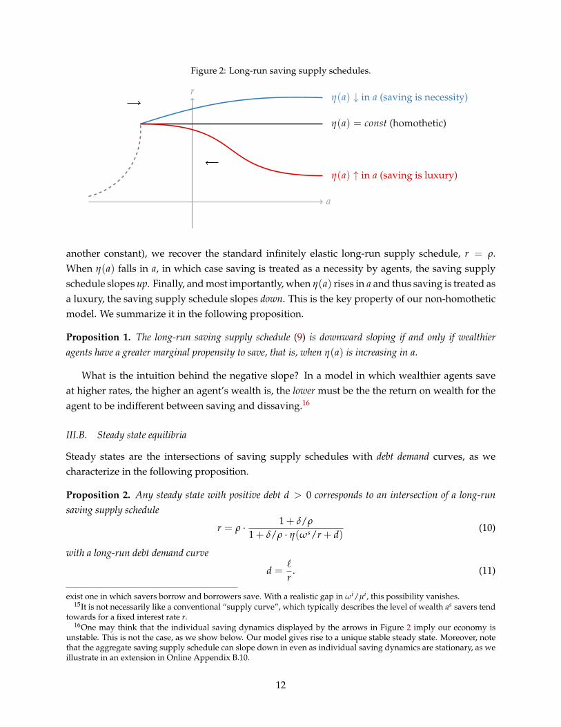
Figure 2: Long-run saving supply schedules.

a

rη(a) ↓ in a (saving is necessity)

η(a) = const (homothetic)

η(a) ↑ in a (saving is luxury)

another constant), we recover the standard infinitely elastic long-run supply schedule, r = ρ.When η(a) falls in a, in which case saving is treated as a necessity by agents, the saving supplyschedule slopes up. Finally, and most importantly, when η(a) rises in a and thus saving is treated asa luxury, the saving supply schedule slopes down. This is the key property of our non-homotheticmodel. We summarize it in the following proposition.

Proposition 1. The long-run saving supply schedule (9) is downward sloping if and only if wealthieragents have a greater marginal propensity to save, that is, when η(a) is increasing in a.

What is the intuition behind the negative slope? In a model in which wealthier agents saveat higher rates, the higher an agent’s wealth is, the lower must be the the return on wealth for theagent to be indifferent between saving and dissaving.16

III.B. Steady state equilibria

Steady states are the intersections of saving supply schedules with debt demand curves, as wecharacterize in the following proposition.

Proposition 2. Any steady state with positive debt d > 0 corresponds to an intersection of a long-runsaving supply schedule

r = ρ · 1 + δ/ρ

1 + δ/ρ · η(ωs/r + d)(10)

with a long-run debt demand curve

d =`

r. (11)

exist one in which savers borrow and borrowers save. With a realistic gap in ωi/µi, this possibility vanishes.15It is not necessarily like a conventional “supply curve”, which typically describes the level of wealth as savers tend

towards for a fixed interest rate r.16One may think that the individual saving dynamics displayed by the arrows in Figure 2 imply our economy is

unstable. This is not the case, as we show below. Our model gives rise to a unique stable steady state. Moreover, notethat the aggregate saving supply schedule can slope down in even as individual saving dynamics are stationary, as weillustrate in an extension in Online Appendix B.10.

12

Figure 3: Steady state equilibrium.

d

r

supply

demand

There is at most one such steady state.

Proposition 2 shows that the relevant saving supply schedule is that of the saver, and that therelevant debt demand curve is given by the borrowing constraint of the borrower. We write bothconditions in terms of the interest rate (return on wealth) r and debt d. Similar to models withdiscount rate heterogeneity, the borrower is up against the borrowing constraint in the steadystate. In this formulation, the debt demand curve slopes down in r. The slope of the savingsupply schedule depends on the slope of η(a). If η(a) is strictly increasing in a, then the savingsupply schedule slopes downward.

We illustrate the saving supply schedule of the saver and the debt demand curve and theirintersection in Figure 3. We prove in Online Appendix A there can only be a single intersection,and hence a single steady state, in the model.17

Steady state in the homothetic economy. In the homothetic economy, the interest rate in the uniquesteady state is necessarily pinned down by the saver’s discount rate, r = ρs. The associated debtlevel is then d = `/ρs.

Analytical example. The steady state conditions in Proposition 2 can be solved analytically in asimple special case, where η(a) is a linear function in the relevant region of the state space. Forexample, assuming η(a) = a, there is a unique stable steady state in this region, with interest rate

r = ρ + δ− δ/ρ(ωs + `)

and associated debt leveld =

`

ρ + δ− δ/ρ(ωs + `).

III.C. Indebted demand

At the core of many of the results in this paper is the idea that an increase in debt service costsby some dx, e.g. caused by a greater level of debt da so that dx = r da, may lower aggregate

17Multiple steady states can occur under more general borrowing constraints (see footnote 11).

13

demand. We next explore this idea starting at the steady state and in partial equilibrium, holdingthe interest rate r fixed.

Proposition 3 (Indebted demand). Assume the economy is in its steady state and hold r fixed. A perma-nent increase dx in debt service costs, or equivalently a permanent transfer from borrowers to savers, movesaggregate spending on impact by

dC = dcb + dcs = −ρ + δ

r12

(1−

√1− 4

(1− r

ρ + δ

)r

ρ + δεη

)dx (12)

Here, εη ≡ η′(a)aη(a) is a measure of the degree of non-homotheticity in preferences. In particular, aggregate

spending falls, dC < 0, if and only if εη > 0.

Proposition 3 highlights that any increase in debt service costs weighs down on aggregatedemand, dC < 0, precisely if and only if εη > 0, a phenomenon we henceforth call indebteddemand.

Why is demand indebted in this case? The increase in debt service costs dx passes throughto the borrower’s spending one-for-one, dcb = −dx. However, since savers have a greater savingpropensity, their spending initially rises by less than the transfer, dcs < dx. Thus, aggregate spend-ing falls, dC < 0. For the goods market to clear, the equilibrium interest rate must therefore fall.As this mechanism only relies on heterogeneity in saving propensities out of a small permanenttransfer dx, any model that generates such heterogeneity along the wealth distribution exhibits theproperty of indebted demand. The model studied in this paper can be regarded as an example ofsuch an economy.

The sign of dC in Proposition 3 is directly related to the slope of the saving supply schedulein Figure 2. The indebted demand property holds, i.e. dC is negative, precisely when saversare situated on a downward-sloping saving supply schedule. This is because, holding r fixed, amarginal increase in wealth da corresponds to a permanent transfer of dx = rda. When savers’consumption dcs responds to this transfer less than one for one, dcs < dx, their saving mustbecome positive, das > 0. But this implies that the shift in wealth da, without an offsetting shift ininterest rates, must have moved savers above their saving supply schedule, into the region wherewealth increases.

Therefore, a downward-sloping saving supply schedule is isomorphic to a marginal propen-sity to consume out of a permanent transfer of less than one. Indebted demand emerges if andonly if the saving supply schedule slopes down. Given the critical role of the slope of the savingsupply schedule in the model, Section IV below provides both microeconomic and macroeco-nomic evidence to support the plausibility of the idea that the the saving supply schedule is infact downward sloping.

The homothetic model, despite its discount rate heterogeneity, has εη = 0 and thus does notgenerate indebted demand. The reason for this is that there is no heterogeneity in saving propen-sities out of a small permanent transfer dx: borrowers do not save out of a small transfer as they

14

are hand-to-mouth; savers do not either as they smooth their consumption perfectly, with r = ρs.As a side remark, observe that our non-homothetic model predicts a positive consumption

response, dC > 0, to a reduction in debt service payments, dx < 0. Such a reduction couldoccur in reality when households refinance their mortgages to bring down the interest rate (“raterefi”). In homothetic models, as εη = 0, there is no effect of “rate refis” on aggregate consumption(Greenwald 2018), which quantitatively limits their macroeconomic relevance (Berger, Milbradt,Tourre and Vavra 2018). In non-homothetic models, such as ours, “rate refis” could instead havesizable consequences for aggregate consumption.

III.D. Transitions

Having discussed the set of steady state equilibria in this economy, we now explore the entire setof equilibria, including the transitions along which the economy approaches the steady state.

The transitions follow along a system of ordinary differential equations (ODEs), with a singlebackward-looking state variable, debt dt, and a single endogenous equilibrium price, the interestrate rt. One can show that borrowers are always up against their borrowing constraint along thetransition unless debt is below some threshold d, which lies below the steady state debt position.Figure 4 illustrates the transitional dynamics in the interest rate - debt space. We next describethe equations characterizing these transitions, for simplicity for the case of a binding borrowingconstraint (that is for dt ≥ d).

Due to the binding borrowing constraint, debt evolves as in (7), that is

dt + λdt = λpt`. (13a)

Here, the price of real assets pt, defined in (5), is the first forward-looking state variable whichfollows the ODE

pt = rt pt − 1 (13b)

The second forward-looking state variable is the consumption of savers, which is determined bythe Euler equation (8)

cst

cst= rt − ρ− δ + δ

cst

ρastη(as

t) (13c)

where wealth of savers can be expressed as ast = ωs pt + dt. Finally, the interest rate is pinned

down by the budget constraint of savers (2), which can be cast as

cst + dt = rtdt + ωs. (13d)

Together, the four equations (13a)–(13d) jointly determine the evolution of the three state variables(dt, pt, cs

t) as well as the interest rate rt.18 It turns out that this evolution is unique for any given

18The three boundary conditions are (a) an initial level of debt d0; (b) the terminal level of the asset price limt→∞ pt =1/r; and (c) the terminal level of savers’ consumption limt→∞ cs

t = cs. r and cs are the steady state values.

15

Figure 4: Equilibrium transitions in the baseline model.

d

r

supply

demandI II

steady state

d

Note. Red: saving supply schedule. Black: debt demand curve. Green: transitional dynamics.

initial level of debt d0 > 0. We verified this using phase diagrams, confirmed it in our numericalsimulations, and provide an analytical local uniqueness & existence result in Online Appendix A.

If d0 is to the left of the steady state (region I), the borrower levers up, hitting the borrowingconstraint as soon as dt crosses d, and ultimately converging to the steady state d. If d0 is to theright of the steady state (region II), interest rates are pushed down relative to steady state, and theborrower has a desire to deleverage. The magnitude of the decline in interest rates in responseto the accumulation of debt depends on the degree of non-homotheticity, as when there is morenon-homotheticity, the saver spends less of the additional debt payments.

Observe that the black line in Figure 4 only corresponds to the borrowing constraint in steadystate, d = `/r. Along the transition from the left, the expectation of lower interest rates in thefuture implies an asset price pt that lies above `/rt. Thus, there can be points (dt, rt) during thetransition that lie to the right of the black line. The opposite happens during transitions from theright.

III.E. Illustrative calibration of the basic model

We next provide an illustrative calibration of our model. The calibration is meant to capture theUS economy in the 1980s, before the recent increase in income inequality. We interpret the saver ascomprising the top 1% earning households of the economy, i.e. with a population share µ = 0.01,and the borrower as the bottom 99%. We choose the saver’s real (non-bond) earnings share ωs tomatch the post-tax income share (excluding returns to household debt) to be consistent with thecalibration of our richer model in Section IX, giving ωs = 0.06. This ensures that the steady statedistribution of income is the same as in our richer model.

We assume an initial interest rate of 5.5%, consistent with an expected real return on wealthof 7.5% (see Figure 1 and discussion in Section II.E.) net of 2% productivity growth. We calibrate` to match the US household debt to GDP level in 1980 of 45%, giving ` = 0.0248. We chooseδ = 0.025 corresponding to an expected duration of a generation of 40 years.19 The discount rateρ, which approximately corresponds to the discount rate of borrowers as the bequest motive is

19This is conservative given the alternative reasons for non-homothetic saving, see e.g. the discussion in Section II.E..

16

less relevant to them, is chosen at 10%. Whenever we refer to the homothetic benchmark model,we use a discount rate of savers of ρs = r = 0.055.

We directly calibrate η(a) = v′(a/µ)a/µ, letting it take a flexible functional form,

η(a) = 1 +1

η alog(

1 + eη(a−a))

(14)

where η, a > 0. This form is arguably the simplest “activation function”, with the followingdesirable properties:20 it is positive and strictly increasing everywhere; it is flat at 1 for low levelsof assets a, implying near-homothetic behavior then; it rises linearly for large asset levels a, withslope a−1; when a→ ∞, η(a) remains flat for all a; the speed at which η(a) moves from flat to linearis parametrized by η; its elasticity εη(a) = η′(a)a

η(a) = 1 − −v′′(a)av′(a) always lies in (0, 1), consistent

with v(a) being a concave function. We jointly calibrate η and a to ensure that the steady stateEuler equation (10) is satisfied and that savers have an MPC out of wealth of 0.01 in line with ourdiscussion in the next section.21

The remaining parameter to be determined is λ, which is less important for our results as itonly matters for the transitional dynamics. It governs the speed of the debt response. To calibrateit, we compare the impulse response of household debt over GDP to a monetary policy shockimplied by our model to that commonly found to identified monetary policy shocks. In particular,we feed a 100 basis point interest rate cut with a half-life of 2 years (similar to (20) below) into theSection VI.B. variant of our model. We compare the household debt / GDP response at its peak(approximately 0.75 percentage points after 2 years) to the response of US household debt / GDPto a Romer and Romer (2004) shock. This procedure implies a λ approximately equal to 0.5.

IV Evidence for a Downward Sloping Saving Supply Schedule

The slope of the long-run saving supply schedule is a crucial aspect of the model. This section pro-vides both microeconomic and macroeconomic evidence supporting the plausibility of a down-ward saving supply schedule among individuals at the top of the income or wealth distribution.

IV.A. Saving rates out of lifetime income

As shown in Figure 2, the saving supply schedule slopes downward in our model if and onlyif η(a), which is the marginal utility of wealth relative to the homothetic benchmark, is strictlyincreasing in a for savers in the economy. In the model, savers are those in the top of the permanentincome distribution, which we interpret as the top 1%. As mentioned in Section II.E., Mian, Strauband Sufi (2020) show that most of the savings in the U.S. economy come from those in the top 1%of the wealth or income distribution. The critical empirical question is whether η(a) is strictlyincreasing in a for those at the top of the distribution.

20The functional form in (14) is a transformation of a “SoftPlus” function commonly used in Machine Learning.

21The formula for the MPC is r− ρ+δ2

(1−

√1− 4

(1− r

ρ+δ

)r

ρ+δ εη

).

17

Empirical research measuring saving rates out of lifetime income can inform us on the slopeof η(a) for the rich. In the homothetic benchmark, saving rates are constant across the lifetimeincome distribution. In contrast, saving rates are rising in lifetime income if η(a) is increasing ina. There is a long line of influential work that supports the view that saving rates out of lifetimeincome are higher for wealthy individuals. For example, this idea features prominently in thewritings of John Atkinson Hobson, Eugen Bohm von Bawerk, Irving Fisher, and John MaynardKeynes, among others. More recently, formal empirical work has validated the notion that savingrates are highest at the top end of the lifetime income distribution.

Dynan, Skinner and Zeldes (2004) use panel data from the Survey of Consumer Finances (SCF)to show that individuals in the top 20% of the income distribution have saving rates out of lifetimeincome that are substantially larger than the rest of the population. The saving rates for the top 1%and top 5% out of income are estimated to be particularly large, almost four times larger than atthe median of the distribution (0.51 compared to 0.13 out of a dollar of permanent income, Table4, column (2)).22

Straub (2019) uses the Panel Study of Income Dynamics (PSID) to estimate an elasticity of con-sumption to lifetime income. If preferences were homothetic, then the elasticity of consumptionwith respect to lifetime income should be one, implying that changes in permanent income in-equality do not impact aggregate consumption. However, the paper estimates that the elasticityof consumption with respect to permanent income is around 0.7, which is evidence in favor of non-homothetic preferences and a concave relationship between consumption and lifetime income.

The advantage of these two studies is that they seek to estimate the saving rate out of lifetimeincome, which is the main object of interest in determining the shape of η(a). In addition, therealso exists recent evidence from studies estimating saving rates out of income more generally.

Fagereng, Holm, Moll and Natvik (2019) use administrative panel data from Norway to es-timate saving rates out of income across the wealth distribution. The study finds substantiallyhigher saving rates for wealthier households, with saving rates for the top 1% estimated to bealmost double the saving rates for the median of wealth distribution.

The empirical strategy of Fisher, Johnson, Smeeding and Thompson (2018) estimates a con-sumption share and after-tax income share of the top 1% of the income distribution of sc = 0.066and sy = 0.171, respectively, for the 2004 to 2016 period. Together with an estimate of the averagepropensity to consume out of income APC in the aggregate, one can estimate the saving rate of thetop 1% as 1− APC · sc/sy = 0.649. Here, the APC is measured as personal consumption expendi-tures divided by disposable personal income from the National Accounts. This same calculationimplies a saving rate of -0.025 for the bottom 99% as a whole. The top 1% have a much highersaving rate than the bottom 99%. In addition to showing a higher saving rate of the top 1%, theSCF evidence also provides further support to the idea that most of the saving in the economy isdone by the top 1%.

22See also the influential article by Carroll (2000) which highlights some of the empirical work on the subject fromthe 1990s.

18

IV.B. MPCs and the return on wealth

The slope of the saving supply schedule can also be discerned through a comparison of the ob-served marginal propensity to consume out of a change in wealth versus the expected return onwealth for the rich. More specifically, let C(r, a) be the steady state consumption of rich householdsin an economy. The definition of the saving supply schedule r(a) as a function of rich households’wealth requires that

C(r(a), a) = r(a)a.

Total differentiation of this equation with respect to a allows us to isolate the local slope of thesaving supply schedule

drd log a

=MPCwealth − r

1− εr(15)

where εr ≡ ∂ log C∂ log r is the elasticity of consumption with respect to a permanent shift in interest

rates, and MPCwealth is the marginal propensity to consume out of wealth for the rich. Given thepreponderance of illiquid wealth among the rich, this ought to be interpreted as the MPC out ofilliquid wealth or capital gains. The denominator of the right hand side is necessarily positive, andso the sign of MPCwealth − r for the rich gives us the local slope of the saving supply schedule.23

Recent studies using data from a number of European countries suggest that the MPCwealth

of the rich is about 1.0%. More specifically, Arrondel, Lamarche and Savignac (2019) estimateMPCwealth across the wealth distribution in France and find that the top 10% has an MPCwealth of0.6%. Garbinti, Lamarche, Lecanu and Savignac (2020) estimate MPCwealth for the top 10% of thewealth distribution across five European countries, and they find estimates of 0.3% for Cyprus,0.6% for Germany, 0.8% for Spain, 1.2% for Belgium, and 2.3% for Italy. Using administrative datafrom Sweden, Di Maggio, Kermani and Palmer (2020) estimate an MPCwealth of 2.8% for the top5% of the wealth distribution. The median and mean of these estimates across countries suggestsan MPCwealth of about 1.0% for those in the top of the wealth distribution.24

How does this compare to r, or the expected return on wealth for the rich? As shown in Figure1, the expected real return on wealth for the U.S. economy as a whole has averaged about 5% from1982 to 2016. It started out at around 7.5% and has fallen to about 3% in recent years. In order toapply it in (15), we need to subtract real GDP growth in the United States, which is about 2%, as(15) was derived in a model without growth. Given these facts on expected returns in conjunctionwith the estimates of the MPCwealth for the top 10% above, the numerator MPCwealth− r is almostassuredly negative, thereby indicating a downward sloping saving supply schedule.

23εr < 1 holds for any function C(r, a) describing the response of initial consumption c0 that is the solution to astandard utility maximization problem with monotone and concave preferences over paths {ct}with prices e−rt relativeto the present and initial wealth a.

24To the best of our knowledge, there are no estimates of how the MPCwealth varies across the wealth distributionin the United States. Chodorow-Reich, Nenov and Simsek (2019) estimate 2.8% in the aggregate. The estimates byGarbinti, Lamarche, Lecanu and Savignac (2020) in other countries suggest an MPCwealth for the bottom 90% that is onaverage five times larger than the top 10%. Applying this pattern to the United States implies that the MPCwealth of thetop of the wealth distribution in the United States is likely to be substantially lower than 2.8%.

19

We can also use formula (15) to get a sense of magnitudes. To do so, we assume εr = 0, whichwould be implied by log preferences.25 Using an estimate of 1% for MPCwealth, and 3% for r netof GDP growth, the average for the United States from 1982 to 2016, we obtain:

drd log a

≈ −2%.

In words, this implies that if the richest households’ wealth rises by 10%, the interest rate has tocome down by 20 basis points. While this is not a precise calculation, it gives a rough sense of themagnitudes that are at play in the model.

IV.C. Evidence using wealth to income ratios

Another implication of higher saving rates of the rich is a positive correlation between top incomeshares and wealth to income ratios.26 This implication is robustly supported by time series data inthe United States, as shown in the left panel of Figure 5. The share of income earned by the top 1%of the income distribution is strongly positively correlated with the aggregate wealth to incomeratio across years from 1913 to 2019.

One may be concerned, however, that other time series factors could have influenced bothinequality and wealth to income ratios in the aggregate. To try to identify the effect of top incomeshares on wealth to income ratios more cleanly, the right panel of Figure 5 uses cross-sectionalvariation across states in the rise in the top 1% share from 1982 to 2007.27 As it shows, there isa strong positive correlation. States in which the top 1% earned a larger share of the state’s totalincome over time also experienced larger wealth accumulation. While the figure only displays acorrelation, Mian, Straub and Sufi (2020) show that this result is robust to variety of controls.28

25Despite log utility over consumption, εr is slightly negative in our model due to the bequest motive in the utilityfunction (1).

26Wealth to income is independent of the lifetime income distribution when saving rates are constant in lifetimeincome (Straub, 2019). Since we do not have data on top lifetime income shares, we use top (current) income shares.We believe this is appropriate given that the rise in (current) income inequality was largely driven by rising inequalityin lifetime income (Kopczuk, Saez and Song, 2010, Guvenen, Kaplan, Song and Weidner, 2017).

27These years are chosen as they are the years for which state-level information is available to construct the wealthto income ratio in a state. See Mian, Straub and Sufi (2020) for more details.

28The slope of the relationship in the time series is larger than the slope of the relationship across states. One reasonfor this is that the time series relationship includes the endogenous response of interest rates to a rise in inequality.If interest rates fall due to a rise in top income shares (as we argue below), then wealth to income ratios will riseeven further. The cross-sectional specification holds fixed the interest rate which is why this endogenous responseis absent in the cross-sectional specification. In this sense, the cross-sectional relationship is the more direct test ofnon-homotheticity without general equilibrium effects.

20

Figure 5: Top Income Shares and Wealth to Income Ratios.

1914

1917

1920

1923

1926

1929

1932

1935

1938

1941

1944

19471950

19531956

19591962

19651968

1971

19741977

19801983

1986

19891992

1995

1998

2001

2004

2007

2010

2013

2016

2019

2

3

4

5

6

We

alth

−to

−in

co

me

.05 .1 .15 .2Top 1% share

National

AL

AK

AZAR

CA

CO

CT

DE

DCFL

GA

HIID

IL

IN

IA

KS

KY

LA

ME

MD MA

MIMN

MS

MO

MT

NE

NV

NH

NJ

NM

NY

NC

ND

OH

OK

OR

PA

RI

SC

SD

TN

TX

UT

VT

VA

WA

WV

WI

WY

0

.5

1

1.5

2

2.5

∆ W

ea

lth

−to

−in

co

me

.05 .1 .15 .2 .25∆ Top 1% share

States

The left panel plots the aggregate wealth to income ratio against the share of income going to the top 1% for the UnitedStates from 1913 to 2019. Every third year is labeled. The data are from Saez and Zucman (2020). The left panel plotsthe change from 1982 to 2007 in the ratio of total household wealth to household income at the state level against thechange in the top 1% share of income over the same period. For full details on data in the right panel, see Mian, Strauband Sufi (2020).

IV.D. Comparing saving supply schedules across models

The evidence is supportive of the view that the saving supply schedule slopes downward for richhouseholds. However, our model does not imply a downward sloping saving supply across theentire distribution. The borrowers in our model are on the upward part of their saving supplyschedule as in other models used in the literature.

Perhaps the most prominent of models with an upward sloping saving supply schedule isAiyagari (1994). In this model, there is a precautionary saving motive for households given thepotential for hitting a borrowing constraint after negative idiosyncratic productivity shocks. In theAiyagari (1994) model, a permanent transfer to households acts as additional insurance, cushion-ing the household in states of low realizations of idiosyncratic productivity. A household thereforeresponds to the transfer by raising consumption more than one for one, decumulating wealth. Asa result, a permanent transfer leads to a lower saving rate.

While this logic is sound for households near a borrowing constraint, it is unlikely to be rel-evant for those near the top of the lifetime income distribution. Such households already haveample resources to buffer negative idiosyncratic shocks, and therefore it is unlikely that they will

21

have lower saving rates if they become richer.29

However, it is important to note that borrowers in our model, which we calibrate to correspondto the bottom 99% of the income distribution, are all on the upward-sloping part of the saving sup-ply schedule, as in Aiyagari (1994). In fact, since debt is negative saving, their downward-slopingdebt demand curve is the exact mirror image of their upward-sloping saving supply schedule. Inour model, the upward slope stems from a borrowing constraint, but as we emphasize in OnlineAppendix B.6, many other formulations are possible, including a precautionary savings motive.

Borrowers are on the upward sloping part of the saving supply schedule while savers are onthe downward sloping part. This is possible despite the fact that all agents share the same prefer-ences. Each agent’s saving supply schedule is first upward-sloping for low levels of wealth nearthe borrowing constraint, and then flattens out as wealth increases. Only if wealth is sufficientlyhigh does it turn down again. Recall from Section II.E. that most of the saving in the U.S. economyover the past 20 years has come from those in the top 1%, which supports the view that most sav-ing in the United States is done by rich households that are likely to be on the downward slopingpart of the saving supply schedule.

V Inequality, Financial Deregulation, and Indebted Demand

The framework developed in the previous sections may help understand the underlying factorsthat contributed to the simultaneous increase in debt and decline in interest rates that many ad-vanced economies have experienced in the past 40 years. We explore this next.

V.A. Inequality

As is well understood by now, many advanced economies have experienced a significant rise inincome inequality (Atkinson, Piketty and Saez 2011). In the model, a rise in income inequality canbe captured as an increasing share ωs of real earnings going to savers, and a corresponding fall inωb = 1−ωs.30 The following proposition characterizes the long-run implications of rising incomeinequality.

Proposition 4. An increase in income inequality (greater ωs) unambiguously reduces long-run equilib-rium interest rates and raises household debt. In the homothetic model, long-run interest rates and house-hold debt are unaffected by rising income inequality.

The long-run implications of rising inequality are best understood in the context of our model’ssaving supply schedule and debt demand curve. Figure 6 shows supply and demand diagrams

29Even in the Aiyagari (1994) model, saving supply schedules go from upward sloping to flat at the highest wealthlevels. The reason is that the precautionary motive ceases to materially influence saving rates for the wealthy. Thereis no force such as non-homotheticity in the Aiyagari (1994) model to generate a downward sloping saving supplyschedule at higher wealth levels.

30The rise in income inequality in the model is a rise in the permanent income of the high endowment agents relativeto the low endowment agents. This experiment matches the data. Both Kopczuk, Saez and Song (2010) and Guvenen,Kaplan, Song and Weidner (2017) show that lifetime income inequality has increased substantially in the United Statessince the early 1980s.

22

Figure 6: The effects of rising income inequality for long-run saving supply and debt demand.

(a) Homothetic model

d

rOld and new steady state

(b) Non-homothetic model

d

r

Old steady state

New steady state

for the homothetic economy in panel (a), and the non-homothetic economy in panel (b). In thehomothetic case, the supply schedule is pinned down by the discount factor and thus independentof inequality. The demand curve is also independent of inequality, and therefore the old and newsteady states coincide.

In the non-homothetic economy, savers have a greater propensity to save. Thus, if they earn agreater share of income, total saving increases. This manifests itself in a shift of the saving supplyschedule (10) to the left: for a given level of debt d, savers earn more resources and are willingto save more. As Proposition 4 shows, and as is illustrated in Figure 6, the equilibrium interestrate falls and the amount of debt in the economy rises in response to the rise in inequality. Thenon-homothetic model thus helps rationalize the close empirical association between the rise ininequality and the simultaneous increase in debt and decline in interest rates across advancedeconomies.

Transition. This is confirmed numerically in Figure 7, which simulates the responses of a homo-thetic and a non-homothetic economy to a permanent increase in income inequality. Since this isa perfect-foresight transition, borrowers begin raising their debt levels already early on, in antici-pation of lower interest rates in the future, which raises demand and thus interest rates initially.31

Interestingly, the transition shows a hump-shaped profile in the debt service ratio, which ul-timately falls back to its pre-transition value. This demonstrates that the debt service ratio is ahighly endogenous object, which can be low either when there is little debt (early in the transi-tion), or, when there is high debt but interest rates are low (late in the transition).

One reaction to the strong increase in debt in Figure 7 may be to point out that in the data,borrowers typically use debt to acquire assets (houses) and that their net worth actually remainedmore or less constant (Bartscher, Kuhn, Schularick and Steins 2020). Shouldn’t this be reflected inthe model?

It turns out that it already is. Clearly, most of the run-up in debt over the last few decades

31Similarly, the homothetic economy shows an on-impact drop in the interest rate, below its initial steady state value(dashed gray line) before converging back to it.

23

Figure 7: Rising income inequality and debt.

0 10 20 30 40 506 %

6.5 %

7 %

7.5 %

8 %

8.5 %

9 %

9.5 %

10 %

years

Top 1% income share

0 10 20 30 40 502 %

3 %

4 %

5 %

6 %

7 %

8 %

years

Interest rate

0 10 20 30 40 50

50 %

60 %

70 %

80 %

90 %

100 %

110 %

years

Household debt / GDP

0 10 20 30 40 501.5 %

2 %

2.5 %

3 %

3.5 %

4 %

4.5 %

years

Debt service / GDP

Homothetic model Non-homothetic model

Note. Plots show transitions from our calibrated steady state with saver income share ωs = 0.06 (dotted gray line) to asteady state with ωs = 0.10. The dashed blue line corresponds to the homothetic model with ρs = 0.055.

is mortgage debt, and thus ultimately collateralized by housing. As we show in our companionpaper, Mian, Straub and Sufi (2020), however, when taken together, the bottom 90% of the wealthdistribution did not use the increase in debt to accumulate more housing. Instead, housing wasbought and sold within the bottom 90%, likely from old homeowners to young homebuyers, andthus ultimately financed consumption expenditure by old homeowners (Bartscher, Kuhn, Schu-larick and Steins 2020). Net worth only remained stable because house prices were rising.

At a stylized level, this is precisely the mechanism in our model. A natural measure of borrow-ers’ financial net worth is their pledgeable wealth net of debt, pt`− dt, where ` can be interpretedas land or housing owned by borrowers. Figure 7 shows how borrowers’ net worth evolves, andsplits it up into its components, pt` and dt. Similar to the data, net worth remains stable in thetransition. Underlying the stability, however, are two opposing trends. On the one hand, pledge-able wealth increased tremendously, as asset prices pt rise; on the other, greater pledgeable wealthrelaxes the borrowing constraint and thus leads to greater debt accumulation.32

32An important caveat here is that this is a perfect foresight transition with rational expectations. In practice, espe-cially in the early 2000s, house prices and borrowing partly increased (and later reversed) due to optimism (see, e.g.

24

Figure 8: Decomposing borrowers’ net worth.

0 10 20 30 40 50−60 %

−40 %

−20 %

0 %

20 %

40 %

60 %

yearsch

ange

rela

tive

tos.

s.ou

tput

Net worth Pledgable wealth Debt

If net worth of borrowers did not change, why then is there indebted demand? Couldn’tborrowers sell their assets, annihilate their debt and finance the same level of consumption asbefore? The answer is no. What matters for borrowers’ consumption stream—and hence theircontribution to aggregate demand—is not their net worth; instead it is their income stream aftermaking debt payments. Valuation effects from lower discount rates and greater asset prices do notalter the income stream. Thus, indebted demand occurs when rich households save and non-richhouseholds dissave; this may or may not coincide with a reduction in borrowers’ net worth.

V.B. Financial deregulation

Another widespread recent trend in advanced economies has been financial liberalization andderegulation. Especially the “mortgage finance revolution” of the 1970s and 1980s allowed newinstitutions to enter mortgage markets, led to securitization of mortgages and to a general loos-ening of borrowing constraints (Ball, 1990). For example, Bokhari, Torous and Wheaton (2013)document large increases in the fractions of mortgages originated with an LTV ratio above 90%and a debt-to-income ratio above 40% from 1986 to 1995. One tension in the literature noted by Jus-tiniano, Primiceri and Tambalotti (2017) and Favilukis, Ludvigson and Van Nieuwerburgh (2017)is that in most standard models, a loosening of such borrowing constraints should be associatedwith an increase in interest rates. We next explore the effects of financial deregulation on debt andinterest rates in the model developed here.

To do so, financial deregulation is modeled as an increase in the pledgability ` of real assets.33

We find the following result.

Proposition 5. Financial deregulation (greater `) unambiguously reduces long-run equilibrium interestrates and increases household debt. By contrast, in the homothetic model, long-run interest rates are unaf-fected by financial deregulation and household debt rises by less.

Kaplan, Mitman and Violante 2020) and relaxed collateral constraints. Both can be captured to some extent by shifts in`. We analyze such shifts in the next section.

33In our housing application in Section B.6.1 we show that a rising LTV ratio amounts to an increase in `.

25

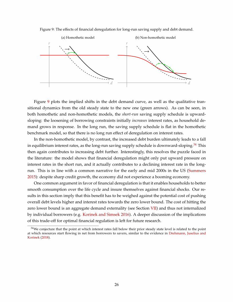
Figure 9: The effects of financial deregulation for long-run saving supply and debt demand.

(a) Homothetic model

d

r(b) Non-homothetic model

d

r

Figure 9 plots the implied shifts in the debt demand curve, as well as the qualitative tran-sitional dynamics from the old steady state to the new one (green arrows). As can be seen, inboth homothetic and non-homothetic models, the short-run saving supply schedule is upward-sloping: the loosening of borrowing constraints initially increases interest rates, as household de-mand grows in response. In the long run, the saving supply schedule is flat in the homotheticbenchmark model, so that there is no long run effect of deregulation on interest rates.

In the non-homothetic model, by contrast, the increased debt burden ultimately leads to a fallin equilibrium interest rates, as the long-run saving supply schedule is downward-sloping.34 Thisthen again contributes to increasing debt further. Interestingly, this resolves the puzzle faced inthe literature: the model shows that financial deregulation might only put upward pressure oninterest rates in the short run, and it actually contributes to a declining interest rate in the long-run. This is in line with a common narrative for the early and mid 2000s in the US (Summers2015): despite sharp credit growth, the economy did not experience a booming economy.

One common argument in favor of financial deregulation is that it enables households to bettersmooth consumption over the life cycle and insure themselves against financial shocks. Our re-sults in this section imply that this benefit has to be weighed against the potential cost of pushingoverall debt levels higher and interest rates towards the zero lower bound. The cost of hitting thezero lower bound is an aggregate demand externality (see Section VII) and thus not internalizedby individual borrowers (e.g. Korinek and Simsek 2016). A deeper discussion of the implicationsof this trade-off for optimal financial regulation is left for future research.

34We conjecture that the point at which interest rates fall below their prior steady state level is related to the pointat which resources start flowing in net from borrowers to savers, similar to the evidence in Drehmann, Juselius andKorinek (2018).

26

VI Implications for Fiscal and Monetary Policy

VI.A. Fiscal policy: Deficits and redistribution

The previous section showed how private deficits lead to the accumulation of household debt,and thus indebted demand. A considerable portion of the recent increase in debt, however, hasbeen public debt. According to conventional wisdom, a rise in government debt exerts upwardpressure on interest rates (e.g. Blanchard 1985, Aiyagari and McGrattan 1998).

What are the implications of a rise in government debt in our non-homothetic model? Thissection focuses on this question in the context of the equilibrium introduced in Section II.D., inwhich output is fixed at Y = 1, and therefore interest rates endogenously adjust to clear the goodsmarket. Section VII revisits fiscal policy in the presence of nominal rigidities and a binding zero-lower bound.

We consider fiscal policy in this section, as well as other policies in subsequent sections, mainlyfrom a positive perspective, documenting its effects in our model without any notion of welfare.The reason for this choice is that there are several real-world considerations that are first-orderfor welfare but outside our model. For example, high debt levels and low interest rates are oftenassociated with instability and risk-taking in the financial sector, and thus raise the likelihood ofa financial crisis (e.g. Reinhart and Rogoff 2009, Schularick and Taylor 2012, Stein 2012). Lowinterest rates may also reduce growth (Liu, Mian and Sufi 2019). Behavioral aspects, such as time-inconsistent preferences, would lead borrowers to accumulate too much debt. One importantdimension of welfare an extension of our model can speak to is the potential for a liquidity trapwhen the (natural) interest rate is sufficiently depressed. We discuss the welfare implications ofour model in this context in Section VII.

Government. We introduce a standard government sector into the economy. Specifically, the gov-ernment is assumed to choose a debt position Bt, government spending Gt, and proportional in-come taxes τi

t on agent i such that its flow budget constraint

Gt + rtBt ≤ Bt + τst ωs + τb

t ωb (16)

is satisfied at all times t. Ponzi schemes are ruled out by assuming that Bt is bounded above,uniformly in t. In the baseline model, government bonds pay the same interest rate as otherassets. We discuss the implications for when this is not the case below.

For simplicity, government spending is treated here as purchases of goods that are eitherwasted, or—which is equivalent for the purposes of this current positive exercise—enter agents’utilities in an additively-separable form. Taxes are assumed to enter agents’ real wealth in thenatural way, rthi

t = (1− τit )ω

i + hi. Taking fiscal policy as given, the definition of a competitiveequilibrium is unchanged from before, with the exception that the bond market clearing conditionis now given by db

t + dst + Bt = 0.

27

Figure 10: Long-run effect of an increase in public debt B.

d + B

r

Long-run effects of fiscal policy. We begin by studying the long-run effects of fiscal policy, focusingon constant policies (G, B, τs, τb). In this case, the equilibrium conditions for steady state equilibriaare given by

r = ρ1 + δ/ρ

1 + δ/ρ · η(a)(17)

a = (1− τs)ωs

r+

`

r+ B (18)

Equations (17) and (18) characterize the long-run implications of fiscal policy. We are specificallyinterested in increases in B, financed by raising taxes τi on both agents or cutting expenditure G;as well as tax-financed increases in G. This yields the following result.

Proposition 6 (Long-run effects of fiscal policy on interest rates and debt.). In the long run,

a) larger government debt (B ↑) depresses the interest rate (r ↓) and crowds in household debt (d ↑).

b) tax-financed government spending (G ↑) increases the interest rate (r ↑) and crowds out householddebt (d ↓).

c) fiscal redistribution (τs ↑, τb ↓) increases the interest rate (r ↑) and crowds out household debt (d ↓).

With a homothetic saver, none of these policies have any effect on the long-run interest rate and on householddebt.

An intuition for these results can be explained with the help of Figure 10. Consider the firstpolicy in Proposition 6, and assume the greater debt level B is entirely paid for by a reductionin government expenditure G. As savers do not raise their consumption one-for-one with theincrease in debt service payments by the government, aggregate demand would fall were it not fora reduction in interest rates. Graphically, the policy corresponds to an increase in the economy’stotal demand for debt, d + B, which shifts out to the right. Notably, the reduction in interest rateswill crowd in household debt.

When the greater level of debt is not paid for by government spending cuts, but instead bygreater taxation, the result in Proposition 6 is qualitatively the same. However, the exact magni-tude of the interest rate decline now depends on the distribution of taxation: in the corner case

28

where borrowers pay all additional taxes, the interest rate decline is as large as when governmentspending is cut; in the corner case where savers pay all additional taxes, interest rates do notrespond.35

Tax-financed government spending and fiscal redistribution reallocate resources from the saverto a “spender”, which is either the government—in the case of government spending—or theborrower—in the case of redistribution. Such resource reallocation would raise aggregate demandwere it not for an increase in interest rates.

Proposition 6 and Figure 10 prescribe a very different role for fiscal policy in influencing inter-est rates than is typically assumed. What helps in the long-run is first and foremost redistributionbetween spenders and savers, not redistribution of taxes over time in the form of public deficits,which, paradoxically, lowers long-run interest rates even further as government demand becomesindebted.

One caveat to Proposition 6 is that the interest rate on government debt B, rB, might differform the interest rate r on other debt d. Here, the result depends on why rB is different from rand, crucially, whether rB is above or below the growth rate, which is zero in the baseline model.For example, it is conceivably that the first result in Proposition 6 breaks when the interest rate ongovernment debt rB lies sufficiently below zero. We leave a characterization of the interaction ofconvenience yields on government debt and indebted demand for future research.

Fiscal policy in the analytical example. We can illustrate the effects of fiscal policy in the analyticalexample in Section III.B.. It is straightforward to obtain the steady state given a set of tax policies(G, B, τs, τb)

r =ρ + δ− δ

ρ ((1− τs)ωs + `)

1 + δρ B

and d =

(1 + δ

ρ B)`

ρ + δ− δρ ((1− τs)ωs + `)

.

G and τb do not enter the expressions, as they are implicitly used to balance the governmentbudget for any values of B, τs; it does not matter which of the two is used. We see that greater re-distribution and greater spending (both financed through greater τs) raises r and lowers d. Greaterpublic debt B lowers r and crowds in d. Finally, greater B reduces the sensitivity of r to changes inτs, ωs or `.

Short run effects. Despite its novel long-run effects of government debt, the model predicts con-ventional short-run effects of debt-financed fiscal stimulus programs (whether through govern-ment spending or tax cuts). As before, in terms of saving supply schedule and debt demandcurve, this is due to an upward-sloping short-run saving supply schedule. We illustrate this in

35Interest rates are constant in government debt when savers are taxed because savers are Ricardian. In a non-Ricardian model with downward-sloping saving supply schedule, e.g. the one in Online Appendix B.9, interest rateswould increase with greater government debt if it is financed by savers alone. Importantly, whether savers are Ricar-dian or not has no bearing on the cases in which borrowers are being taxed or the government cuts back its spending.

29

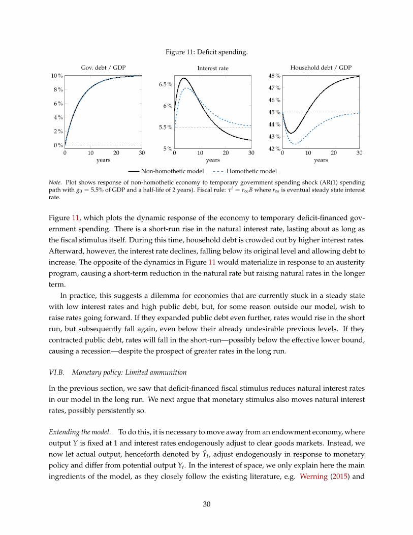
Figure 11: Deficit spending.

0 10 20 300 %

2 %

4 %

6 %

8 %

10 %

years

Gov. debt / GDP

0 10 20 305 %

5.5 %

6 %

6.5 %

years

Interest rate

0 10 20 3042 %

43 %

44 %

45 %

46 %

47 %

48 %

years

Household debt / GDP

Non-homothetic model Homothetic model

Note. Plot shows response of non-homothetic economy to temporary government spending shock (AR(1) spendingpath with g0 = 5.5% of GDP and a half-life of 2 years). Fiscal rule: τi = r∞B where r∞ is eventual steady state interestrate.

Figure 11, which plots the dynamic response of the economy to temporary deficit-financed gov-ernment spending. There is a short-run rise in the natural interest rate, lasting about as long asthe fiscal stimulus itself. During this time, household debt is crowded out by higher interest rates.Afterward, however, the interest rate declines, falling below its original level and allowing debt toincrease. The opposite of the dynamics in Figure 11 would materialize in response to an austerityprogram, causing a short-term reduction in the natural rate but raising natural rates in the longerterm.

In practice, this suggests a dilemma for economies that are currently stuck in a steady statewith low interest rates and high public debt, but, for some reason outside our model, wish toraise rates going forward. If they expanded public debt even further, rates would rise in the shortrun, but subsequently fall again, even below their already undesirable previous levels. If theycontracted public debt, rates will fall in the short-run—possibly below the effective lower bound,causing a recession—despite the prospect of greater rates in the long run.

VI.B. Monetary policy: Limited ammunition

In the previous section, we saw that deficit-financed fiscal stimulus reduces natural interest ratesin our model in the long run. We next argue that monetary stimulus also moves natural interestrates, possibly persistently so.

Extending the model. To do this, it is necessary to move away from an endowment economy, whereoutput Y is fixed at 1 and interest rates endogenously adjust to clear goods markets. Instead, wenow let actual output, henceforth denoted by Yt, adjust endogenously in response to monetarypolicy and differ from potential output Yt. In the interest of space, we only explain here the mainingredients of the model, as they closely follow the existing literature, e.g. Werning (2015) and

30

Auclert, Rognlie and Straub (2018). We describe the full model extension in great detail in OnlineAppendix B.7.

To allow output Yt to be endogenous, we assume it is produced using efficiency units of laborNt, Yt = Nt, which are supplied by both types of agents. We assume that dynasty i has laborproductivity ωi and supplies hours ni

t, such that total labor units are Nt = ωbnbt +ωsns

t . We modifydynasty i’s utility function to include a standard additively separable disutility from labor supply.Dynasty i’s total real asset wealth hi

t is now given by its human capital, hit =

∫ ∞t e−

∫ st ruduωini

sds,so that dynasty i’s budget constraint simply becomes

cit + rtdi

t ≤ dit + ωini

t.

We follow Werning (2015) and Auclert, Rognlie and Straub (2018) in assuming that prices areflexible, nominal wages are perfectly rigid, and that aggregate labor demand Nt is allocated acrossagents using a simple uniform allocation rule, namely ni

t = Nt.36 This implies that real earningsby type i are ωiYt, and thus that the income distribution is unaffected by the level of aggregateoutput Yt. Moreover, as we show in Online Appendix B.7, the disutility can be specified such thatthe allocation with Yt = Nt = ni

t = 1 is the natural allocation. We continue to denote potentialoutput by Yt = 1.

To ensure continued tractability of the model, we treat monetary policy as controlling the realrate directly, as in Werning (2015), McKay, Nakamura and Steinsson (2016) and Auclert, Rognlieand Straub (2020).37 Transmission of monetary policy then works in the standard way: monetarypolicy changes the interest rate, which steers aggregate demand and thus output (and labor) inthe economy. With exogenous interest rates {rt}, the goods market now clears because {Yt} isendogenous. We define as natural interest rates the sequence of real interest rates {rn

t } that achievesthe natural allocation, that is, it implements a path of aggregate demand at potential, Yt = Y = 1.Given the assumptions above, this model is “backwards compatible”, in that its natural allocationprecisely corresponds to our baseline model from Section II.

Monetary policy shocks. We consider two types of monetary policy shocks, which hit the economyat a stable steady state (cb, cs, r, d). The first type is a T-period long interest rate reduction, beforea reversal back to the original interest rate

rt =

r t ≤ T

r t > T. (19)

36The precise formulation of wage stickiness is actually irrelevant for this section as we make the simplifying as-sumption below that monetary policy sets the real interest rate directly. See Auclert, Rognlie and Straub (2018) for arelated argument.

37This corresponds to a Taylor rule with a Taylor coefficient of 1. One can easily study other Taylor coefficients, afterspecifying the wage Phillips curve. The transmission from real rates to real economy outcomes remains unaffected.Note that, different from a textbook New-Keynesian model, our economy is locally determinate under a real-rate rule.

31

The second type also starts with a T-period long interest rate reduction, but then reverses back tothe path of natural interest rates

rt =

r t ≤ T

rnt t > T

, (20)

ensuring that for any t > T after the intervention Yt = Y = 1 in this case.

Monetary policy and debt. We begin by studying monetary policy shocks of the first kind. Inour model, they stimulate the economy via two separate channels. First, they relax borrowingconstraints and encourage borrowers to use additional household debt for spending (debt chan-nel). Second, through income and substitution effects, they provide incentives for savers to spendmore (saver channel). To study the role of these channels for monetary transmission, we define thefollowing present values

PVτ({cit}) =

∫ τ

0e−∫ t

0 rsdscitdt−

∫ τ

0e−rtcidt

PVτ({Yt}) =∫ τ

0e−∫ t

0 rsdsYtdt−∫ τ

0e−rtYdt

The first is the increase in the present value of agent i’s spending until period τ; the second is theincrease in the present value of output until period τ. The next proposition shows that the twochannels have asymmetric implications for the path of aggregate demand.

Proposition 7. The τ-period present value of the output response to the monetary policy shock (19) is givenby

PVτ({Yt}) =1

ωs PVτ({cst})︸ ︷︷ ︸

saver channel

+1

ωs e−∫ τ

0 rsds (dτ − d)︸ ︷︷ ︸debt channel

. (21)

In the long run (τ = ∞), the present value of output is entirely determined by the saver channel,

PV∞({Yt}) =1

ωs PV∞({cst}). (22)

This implies that any output stimulus generated by debt accumulation necessarily weighs negatively onoutput going forward.

Proposition 7 shows that the two channels of monetary transmission have vastly differentimplications for the path of output. While the saver’s consumption response to the interest ratechange affects output permanently, the debt channel only has a temporary effect. In fact, as any ad-ditional debt taken out by borrowers eventually has to be serviced or even repaid, future demandis reduced by an active debt channel. Put differently, when monetary policy is used to stimulatethe economy, any resulting increase in demand that is debt-financed does not sustainably raisedemand and will contribute to reduced demand in the future.

One implication of the result in Proposition 7 is that if monetary policy is accommodative now,

32

Figure 12: Debt limits the ammunition of monetary policy.

t

r

r

T

full

amm

unit

ion

monetaryintervention

possible naturalinterest rate paths

mor

ede

bt,

grea

ter

ε η

redu

ced

amm

o.

it endogenously limits its room to be accommodative in the future, as it also needs to ensure thatthe accumulated debt burden from past interventions does not cause a shortfall in demand. Theaccurate object summarizing the “room to be accommodative in the future” is the natural rate ofinterest rn

t . Our next proposition studies the effect that monetary policy has on rnt .

Proposition 8. To first order, a monetary policy shock as in (19) or (20) causes debt to rise and the naturalrate to fall, rn

t < r for any t. For a given increase in debt, the natural rate falls by more (as measured by∫ ∞s e−r(t−s)rn

t dt for any s) if there is more non-homotheticity (as measured by the elasticity εη of η); and ifinterest rates are lower (lower r) for longer (larger T).

Accommodative monetary policy systematically reduces natural interest rates in our model,and thus endogenously limits the “ammunition” that is available to monetary policy in the future,before economy approaches the effective lower bound. This happens because in the presence ofa greater debt burden, natural rates rn

t cannot possibly be equal to r after t = T as this wouldtighten borrowing constraints, and lead to the borrower severely contracting demand. Therefore,natural rates rn

t are below r at least for some time after t = T while the borrower deleverages (seeFigure 12).

This logic operates even absent non-homotheticity. However, in a homothetic model, the con-vergence process rn

t → r is sped up significantly by the fact that the saver’s consumption risessignificantly due to the increase in the saver’s permanent income, pushing the natural rate up,closer to r. In a non-homothetic model such as ours, an additional reason for a decline in rn

t

emerges—indebted demand—which leads to lower natural rates and a significantly reduced con-vergence rate back to r. In other words, non-homotheticity and indebted demand significantlyaggravate the “limited ammunition” property of monetary policy (see Figure 12). This can besufficiently strong to permanently lower natural rates. Such behavior occurs when the economyexhibits multiple steady states (see our discussion in Section III.B.), and the monetary interventionis “too low for too long”, that is, r is sufficiently low and T sufficiently long.

33

Relationship to literature. A number of economists have recently emphasized how the effective-ness of monetary policy interventions can be reduced by past interventions (e.g. Eichenbaum,Rebelo and Wong 2019, Berger, Milbradt, Tourre and Vavra 2018). In this paper, we do not con-sider consecutive interventions. Instead, we focus on how much “ammunition” in terms of thenatural interest rate, a single intervention costs. This aspect of our paper is closest to McKay andWieland (2019). To give an analogy with the IS curve, we focus on the effect of monetary policyon the future level of the IS curve as opposed to its slope.38

Practical implications for the conduct of monetary policy. Monetary policy can have long-lasting ef-fects on natural rates through the accumulation of debt. This should be taken into account whencontemplating the force with which to respond to different kinds macroeconomic shocks. Tem-porary shocks to borrowers’ ability to borrow for instance—e.g. during a financial crisis—can bemet with aggressive monetary easing as debt is unlikely to rise in this context. However, whenreacting to shocks that do not directly affect borrowers’ demand for debt—e.g. negative shocksto business investment as during the 2001 recession—aggressive monetary policy could lead tosignificant and persistent increases in household debt, and therefore reduce monetary policy am-munition going forward.

When used in conjunction with macroprudential policies that are designed to keep debt incheck, thereby dampening the debt channel, monetary policy can be used more aggressively. Thatway, the economy does not merely “pull forward” demand through debt, demand which it thenlacks in the future.

VII Debt Trap and Policies to Escape It

The most serious implications of indebted demand occur when it tips the economy into a liquiditytrap. We next discuss ways in which an economy can slide into a liquidity trap, and evaluate policyoptions that may help the economy recover.

To do so, we focus on the case of our model where the interest rate associated with our model’ssteady state is possibly below its effective lower bound (ELB). Let r > 0 denote that (real) effectivelower bound. It needs to be positive as we take r to be the real return on wealth in our model.To get a number for r, we propose to take an estimate of the real return on wealth during theELB period—e.g. around 3.5% in Figure (1)—which then needs to be de-trended by productivitygrowth during the ZLB episode—e.g. 1.5%—to obtain r. In this example, r = 2%.39

We next study a situation where the steady state natural interest rate r lies below r, so thatmonetary policy cannot achieve full employment in steady state.

38Aside from these implications, our model also finds that forward guidance is less powerful than in standard New-Keynesian models, for a reason similar to the one in Michaillat and Saez (2019).

39r can be microfounded in the context of our model in Online Appendix B.2, where it would be equal to the conve-nience yield. In Online Appendix B.8, we show how allowing for wage deflation amplifies our findings.

34

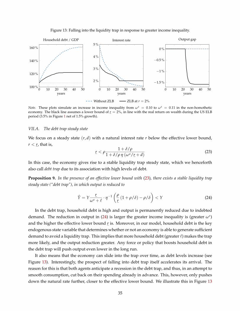
Figure 13: Falling into the liquidity trap in response to greater income inequality.

0 10 20 30 40 50100 %

120 %

140 %

160 %

years

Household debt / GDP

0 10 20 30 40 50

2 %

3 %

4 %

5 %

years

Interest rate

0 10 20 30 40 50

−1.5 %

−1 %

−0.5 %

0 %

years

Output gap

Without ZLB ZLB at r = 2%

Note. These plots simulate an increase in income inequality from ωs = 0.10 to ωs = 0.11 in the non-homotheticeconomy. The black line assumes a lower bound of r = 2%, in line with the real return on wealth during the US ELBperiod (3.5% in Figure 1 net of 1.5% growth).

VII.A. The debt trap steady state

We focus on a steady state (r, d) with a natural interest rate r below the effective lower bound,r < r, that is,

r < ρ1 + δ/ρ

1 + δ/ρ η (ωs/r + d)(23)

In this case, the economy gives rise to a stable liquidity trap steady state, which we henceforthalso call debt trap due to its association with high levels of debt.

Proposition 9. In the presence of an effective lower bound with (23), there exists a stable liquidity trapsteady state (“debt trap”), in which output is reduced to

Y = Yr

ωs + `· η−1

(ρ

r(1 + ρ/δ)− ρ/δ

)< Y (24)

In the debt trap, household debt is high and output is permanently reduced due to indebteddemand. The reduction in output in (24) is larger the greater income inequality is (greater ωs)and the higher the effective lower bound r is. Moreover, in our model, household debt is the keyendogenous state variable that determines whether or not an economy is able to generate sufficientdemand to avoid a liquidity trap. This implies that more household debt (greater `) makes the trapmore likely, and the output reduction greater. Any force or policy that boosts household debt inthe debt trap will push output even lower in the long run.

It also means that the economy can slide into the trap over time, as debt levels increase (seeFigure 13). Interestingly, the prospect of falling into debt trap itself accelerates its arrival. Thereason for this is that both agents anticipate a recession in the debt trap, and thus, in an attempt tosmooth consumption, cut back on their spending already in advance. This, however, only pushesdown the natural rate further, closer to the effective lower bound. We illustrate this in Figure 13

35

by plotting the transition path without imposing an ELB, which crosses the ELB later (blue dashedline).

The presence of debt as endogenous state variable sets our model apart from several promi-nent recent papers modeling secular stagnation, e.g. Benigno and Fornaro (2018), Caballero andFarhi (2017), Eggertsson, Mehrotra and Robbins (2019), and Ravn and Sterk (2020). Moreover, theliquidity trap here is indeed a trap, meaning associated with a stable steady state, rather than arelatively brief episode driven by household deleveraging, as in Eggertsson and Krugman (2012)and Guerrieri and Lorenzoni (2017).

VII.B. Potential policies to escape the trap

Fiscal policy in the debt trap. Once an economy finds itself in the debt trap, how does it get backout again? We can formally introduce the government exactly as in Section VI.A. and obtain thefollowing result.40

Proposition 10. With proportional income taxes τs, τb on the saver and borrower, output in the debt trapsteady state is given by

Y = Yr

(1− τs)ωs + `· η−1

(ρ

r(1 + ρ/δ)− ρ

δ

)(25)

In particular, greater redistribution through taxes raises output and greater tax-financed government spend-ing raises output.

This result is the mirror image of Proposition 6, except that at the effective lower bound, ad-justments in the natural rate correspond to adjustments in aggregate demand and output. Inparticular, Proposition 10 suggests that redistributive tax policies—greater τs—can raise outputY, reducing the severity of the liquidity trap. What would be the consequences of such a policyfor the two agents? As long as the effective lower bound still binds, steady state consumption andwealth are given by

cs = rη−1(

ρ

r(1 + ρ/δ)− ρ

δ

)Y, as =

cs

r, cb = Y− cs. (26)

The only object that is endogenous to the tax choice is Y. Remarkably, greater redistribution there-fore leaves the steady state consumption and wealth of savers entirely unaffected, while boostingthe consumption of borrowers. The reason for this result is that the income loss of greater taxationof savers’ incomes is exactly offset by rising overall incomes. This can happen in the liquidity trapdue to aggregate demand externalities, as in Korinek and Simsek (2016) and Farhi and Werning(2016).

40We leave out policies related to government debt here as those require a well-microfounded model of the interestrate spread between government and private debt that is beyond the scope of this paper.

36

What are the implications for welfare? While (26) only holds across steady states, observethat any policy change that raises Y also relaxes the borrowing constraint and thus generatesadditional consumption for borrowers during the transition period. Moreover, one can show thatconsumption and wealth of savers are constant at the levels in (26) throughout the transition.Thus, our model implies that, in the liquidity trap, greater redistribution is Pareto-improving.

Wealth taxes. Our framework provides an interesting and novel perspective to the current debate(as of January 2021) surrounding wealth taxes (e.g. Saez and Zucman 2019, Guvenen, Kambourov,Kuruscu, Ocampo-Diaz and Chen 2019, Sarin, Summers and Kupferberg 2020). A (progressive)wealth tax τa in our model taxes the saver’s wealth as = d+ ωs

r + B each period, that is, the savers’consolidated budget constraint (2) becomes

cst + as

t = (rt − τa) ast (27)

The returns to this policy are rebated to borrowers. As can be seen in (27), the wealth tax effectivelyreduces the after-tax return on wealth realized by savers. This changes their steady state savingsupply schedule (9) to

r− τa = ρ · 1 + δ/ρ

1 + δ/ρ · η(as)

The relevant interest rate for savers’ saving behavior is the after-tax return on wealth r− τa. Thus,the presence of τa effectively relaxes the effective lower bound, raising output (25) during theliquidity trap according to

Y = Yr− τa

(1− τs)ωs + `(r)· η−1

(ρ

r− τa (1 + ρ/δ)− ρ

δ

).

Thus, a progressive wealth tax is successful in mitigating the impact of secular stagnation in ourframework.41

Macroprudential policies in the debt trap. A commonly prescribed remedy for economies with highdebt burdens is macroprudential policy designed to bring down debt. Being the opposite of finan-cial deregulation, we think of such a policy as a reduction in `. Equation (24) immediately impliesthat such a policy raises demand and output Y in the long run, mitigating the recession. However,during the period of deleveraging, the economy goes through a significant short-run bust. Thisemphasizes that debt is best reduced by reducing saving supply rather than the demand for debt.

Debt jubilees. An alternative way to deal with a liquidity trap caused by high levels of debt is adebt jubilee. We define a debt jubilee of size ∆ > 0 as an immediate reduction in both private debt dand saver’s assets as by ∆. The following result lays out the long-run implications of a debt jubilee

41Interestingly, our model also suggests that a consumption (or VAT) tax would reduce natural interest rates andhence worsen the liquidity trap.

37

policy:

Proposition 11 (Bailouts and debt jubilee.). A debt jubilee raises output in the short run, but unlesscombined with structural changes to inequality, redistribution or debt limits, there is no change to theeconomy in the long-run.

A debt jubilee amounts to a sudden reduction in the state variable dt. With a unique stablesteady state, this cannot have a long-run effect. In other words, borrowers would get themselvesinto debt again. However, a debt jubilee has positive short run effects, as it lifts the economytemporarily out of the debt trap. To prevent it from falling into it again, it can be paired withother policies, e.g. redistributive or macroprudential policies (see above). Such a combination canjointly address short and long-run issues.

VIII Two Extensions

Our baseline model was intentionally kept simple. We now present two extensions to the baselinemodel in Section II, beginning with investment.42

VIII.A. Role of Investment

To introduce investment, we allow output Y to be produced from three factors, capital K and bothtypes of agents’ labor supply ni, and we write the net-of-depreciation production function as43

Y = F(K, nb, ns).

Dynasty i is assumed to have a labor endowment of ni = 1 whose factor income is capitalized in itsreal asset wealth, or human capital, hi

t.44 We assume without loss of generality that Y has constant

returns to scale; otherwise we include a fixed factor owned by savers and/or borrowers. Thus,total income Y can be split up into income going to savers and income going to borrowers. Theincome shares only depend on the level of capital K, which itself is pinned down by the interestrate,

FK = r.

As only savers hold capital in our economy, the agents’ income shares are then described by thefollowing functions of the interest rate

ωs(r) =FKK

F+

Fns ns

Fand ωb(r) =

Fnb nb

F= 1−ωs(r).

42Online Appendix B shows a number of other important extensions.43We assume the typical: F is strictly concave, satisfying Inada conditions.44We assume that the economy is not in the debt trap for this section. Investment would be negatively affected in the

debt trap and thus amplify the output loss there, similar to the logic in Benigno and Fornaro (2018).

38

Figure 14: Capital and indebted demand.

d

r

σ = 1σ > 1

σ < 1

With these income shares, we can now characterize our economy’s steady states as

r = ρ · 1 + δ/ρ

1 + δ/ρ · η(ωs(r)/r + d)and d =

`

r. (28)

Crucially, ωs(r) is now possibly a function of r. As we demonstrate in the following proposition,the shape of ωs(r) depends on the (Allen) elasticity of substitution σ ≡ Fnb FK/(FKnb F) betweencapital and borrowers’ labor supply.

Proposition 12. Let σ be the elasticity of substitution between capital and borrowers’ labor supply in theeconomy with investment. Denote by ωs(r) the savers’ income share.

a) If σ = 1: ωs(r) is independent of the interest rate r. The steady state is identical to the one in theeconomy without investment.

b) If σ < 1: ωs(r) falls with lower r. This flattens the saving supply schedule.

c) If σ > 1: ωs(r) rises with lower r. This steepens in the saving supply schedule.

Proposition 12 precisely characterizes the role of investment for the long-run economy. Whenan increase in capital leaves the income distribution unchanged, investment will have no effect inthe long-run (case (a)). The extent to which capital matters depends on whether it crowds the shareof income going to borrowers in or out. If capital is complementary to borrowers’ labor supply, itreduces the extent of indebted demand (even if it can never fully undo it) as lower interest rates gohand in hand with greater capital and a more equitable income distribution (case (b)). If capital issubstitutable with borrowers’ labor supply—one may think of capital-skill complementarity andautomation as in Krusell, Ohanian, Rios-Rull and Violante (2000) and Autor, Levy and Murnane(n.d.)—the opposite is the case. Lower interest rates endogenously lead to a more unequal incomedistribution, effectively steepening the saving supply schedule and amplifying the problem ofindebted demand (case (c)).45 We illustrate the three cases in Figure 14.

This discussion focused on the long run. Investment contributes to demand in the short runas interest rates fall, irrespective of the structure of the production function F. For example, if F

45See Straub (2019) for a related point.

39

is Cobb-Douglas, and the economy sees a shift in income inequality, investment picks up initially,temporarily slowing the decline in r. As the investment boom recedes, however, the fall in raccelerates again, eventually falling to the exact same steady state level as would have occurredwithout investment (as in Section V).

Observe that the recent US experience does not align well with this description of investment.It did not seem that investment (as a fraction of GDP) rose as interest rates fell. This is subject ofa recent literature (e.g. Gutierrez and Philippon 2016, Liu, Mian and Sufi 2019, Farhi and Gourio2018, Eggertsson, Robbins and Wold 2018).

Which kind of debt causes indebted demand? Productive vs. unproductive debt. Investment may befunded with (corporate) debt, raising the question, which kind of debt actually causes indebteddemand? In Section III, we argued that, starting in some steady state, a one-time exogenousincrease in debt by some dD, holding r fixed, causes a response of aggregate spending of

dC = −ρ + δ

2

(1−

√1− 4

(1− r

ρ + δ

)r

ρ + δεη

)dD (29)

(see Proposition 12). The debt in this experiment is unproductive, that is, it is being used for con-sumption.

We now repeat this exercise with productive debt, that is, debt that is being used to raise thecapital stock of the economy, dK = dD. Holding r and household debt d fixed, what are theimplications for aggregate spending?

Proposition 13 (Indebted demand when debt is productive). Starting from a steady state and holdingr and d, fixed, an exogenous increase in debt dD that raises the capital stock by the same amount affectsaggregate spending by

dC = −ρ + δ

2

(1−

√1− 4

(1− r

ρ + δ

)r

ρ + δεηχ

)dD. (30)

where χ ≡(1− σ−1)ωb − r rd

Y < 1.

A first observation about Proposition 13 is that productive debt, (30), always causes strictlyless indebted demand than unproductive debt, (29). To see this, note that χ =

(1− σ−1)ωb −

r rdY < 1. Thus, even if capital is perfectly substitutable with borrowers’ labor supply, σ = ∞,

productive debt does not cause as much indebted demand. The reason for this is that even ifσ = ∞, capital raises aggregate output. A second observation is that the negative effect of dD onaggregate spending dC falls for lower values of σ, as one would expect given Proposition 12. Inthe case σ = 1, the effect is positive at first, dC > 0. Recall that (30) is the contemporary effect onspending—but once we allow household debt to increase with Y, the positive effect fades.

The distinction between productive and unproductive debt is not always obvious. Consider,for example, investment in infrastructure (e.g. airports, buildings, public transport) in remote

40

locations, as some argue can be found in China today. Debt that is financing such investmentsought to be thought of as unproductive.

A special case where debt is used productively but χ is still very high is residential investmentinto borrowers’ owner-occupied housing. For example, imagine borrowers remodel or extendtheir houses. Clearly this is productive, as a greater housing stock produces more housing ser-vices. However, these additional housing services are consumed by borrowers themselves and donot increase borrowers’ marginal product of labor. Thus, in this case, σ = ∞ and χ = ωb − r rd

Y ,the largest possible value for productive debt.

In sum, our results suggest that productive debt always causes weaker indebted demand thanunproductive debt. The degree to which it is weaker depends on the elasticity of substitution σ

between the capital that is accumulated using debt and the borrowers’ labor supply. This suggeststhat debt-financed productive investments made by firms or governments need not necessarilycontribute to indebted demand.

Does student debt contribute to indebted demand? Since the end of the Great Recession, the US haswitnessed a significant increase in student debt, begging the question whether student debt is alikely contributor to indebted demand. At the face of it, it seems that the answer is no. After all,student debt finances investment in human capital, and thus can be analyzed like investment inphysical capital.

There is, however, an important difference. The rise in student debt partly reflects the risingcost of college tuition. To the extent that this is the case, student debt is indeed a source of indebteddemand, as borrowers have to service larger piles of student debt without having accumulatedgreater human capital.

VIII.B. Longer duration debt

A recent literature highlighted that responses of economies to interest rate changes differ accord-ing to the type of debt contract agents hold (e.g. adjustable-rate vs. fixed-rate contracts) as well asthe debt’s maturity (e.g. Campbell 2013, Calza, Monacelli and Stracca 2013, Di Maggio et al. 2017).In this extension, we briefly investigate the conceptual role of debt duration for indebted demand.

Consider a version of our baseline model in Section II. Assume debt has an entirely fixed rate,equal to the steady state debt payment ` (which is equal across steady states). How does thischange the economy?

While fixed rate (FR) debt does not change the steady state, it does affect the transitional dy-namics. To show this, consider first the experiment of rising income inequality in Figure 7. In thatfigure, due to the anticipated fall in interest rates, the present value of pledgeable wealth increases,while the present value of debt remains unchanged, as debt is adjustable rate. Thus, borrowershave more room to spend, pushing interest rates up in the short run.

With fixed rate debt, the present value of debt jumps on impact, in lockstep with pledgeablewealth. In fact, given our assumption of completely fixed debt, the value of debt exactly equals

41

pledgeable wealth. This implies that borrowers have no additional room to spend, and the econ-omy adjusts immediately on impact.

Proposition 14 (Transition with completely fixed rate debt.). When debt carries a completely fixed rate`, an unexpected permanent change in income inequality (greater ωs) lets the economy jump immediatelyto its new steady state.

Thus, the presence of fixed rate debt implies weaker aggregate demand during transitions withrising debt levels and falling interest rates, which speeds up the transition.

Now consider a shock that pushes real interest rates up, such as a reduction in inequalityor an increase in progressive taxation. The present value of adjustable-rate (AR) debt is againunchanged, but the present value of FR debt falls, again speeding up the transition. Thus, in thissense, AR debt makes it harder to leave a steady state with high levels of debt since any increasein interest rates leads to an immediate sharp fall in demand without favorable revaluation effect.

These discussions highlight that AR debt contracts slow down transitions into states with lowr and high debt, and FR debt contracts speed up transitions away from such states. Fixed-ratecontracts with automatic refinancing achieve both of these arguably favorable outcomes.46 Policiesthat raise the share of refinancing among US fixed-rate mortgage owners are therefore beneficialfrom this perspective.

IX Quantitative Exploration

Thus far, we illustrated several important properties in various extensions of the baseline model.In this section, we combine those extensions into a single richer model. Relative to the baselinemodel in Section II, the model in this section includes additional forces: taxation and governmentbonds in the steady state; land; investment subject to Hayashi (1982) type capital adjustment cost;and the possibility of a transition without perfect foresight. We use the model to revisit the effectof inequality on interest rates and debt.

Extending the model. Households — Dynasties continue to maximizes preferences (1), subject totheir budget constraints (2). Their wealth ai

t is still given by hit− di

t. Real asset wealth is now givenby the discounted stream of after-tax human wealth as well as the dynasty’s share κi of capitalholdings

hit =

∫ ∞

te−∫ s

t rudu(1− τis)wsµ

inisds + κi Jt

where κs + κb = 1; Jt is the value of land and capital combined. We continue to assume that agentscan pledge part of their real asset wealth, in this case part of their land holdings, giving rise to thesame borrowing constraint (7), in which pt is the price of land.

46Lengthening the maturity of debt when debt is high, as in Campbell, Clara and Cocco (2020), would further speedup transitions back to lower debt states as they would lengthen the duration of debt. Automatic refinancing is reminis-cent of the idea to convert FR into AR contracts (Guren, Krishnamurthy and McQuade 2021), albeit such a conversionwould slow down transitions back to states with lower debt levels.

42

Government — The government finances a fixed amount of government spending G and afixed amount of government debt B using proportional taxes τi

t = τt that are set to satisfy thegovernment budget constraint (16).

Investment — There is a representative firm making investment decisions subject to quadraticcapital adjustment costs. The firm uses a nested CES production function of the form

Y = F(L, K, nb, ns) = Lψ

(α

α + ωb

(KK∗

) σ−1σ

+ωb

α + ωb

(nb) σ−1

σ

) σσ−1 (α+ωb)

(ns)ωs

where ψ is the share of income going to owners of land L and, as before, σ is the Allen elasticitybetween K and nb.47 The normalization parameter K∗ will be chosen to be equal to the initialsteady state capital stock, in order for there not to be a direct effect of changes in σ on output.When σ = 1, the production function is Cobb-Douglas, with capital share α and labor incomeshares ωi. We assume ψ + α + ωb + ωs = 1. The firm maximizes its value

rt Jt(Kt) = maxnb

t ,nst ,It

F(Kt, nbt , ns

t)− wbt nb

t − wst n

st − It − ζ

(It − δKKt

Kt

)Kt +

ddt

Jt(Kt) (31)

subject to the law of motion of capital Kt = It − δKKt. The adjustment cost function is quadraticζ(x) = 1

2δKεKx2. The price of capital is given by pt ≡ ∂Jt(Kt)/∂Kt.

Equilibrium — The definition of equilibrium is like in Section II.D.. Households maximize theirutility (1), firms maximize their value (31), and markets clear:

cst + cb

t + It + G = Yt dst + db

t + B = 0.

Calibration — We pursue a similar calibration strategy to the one in Section III.E.. We continueto use the same values for µ, ρ, δ, `, r, λ. The land share is set to ψ = 0.05, depreciation δK is set to0.06, and the capital share α is set to 0.20, so that the value of capital to output is approximately 2.5in the steady state, a standard value. Government spending G is 15% of GDP, government debtis 40% of GDP. Parameters η, a are still chosen to match a steady state interest rate of 5.5% andan MPC out of wealth of savers of 0.01. Here, this gives η = 1.14, a = 0.51. ωs and κs, which forsimplicity we choose to be the same, are picked to match a top 1% income share of 10% (Smith,Yagan, Zidar and Zwick 2019) in 1980. This gives ωs = κs = 4%.48 The adjustment cost parameterεK is chosen to match a semi-elasticity of investment to Tobin’s Q, pt, of 1 as in Auclert and Rognlie(2018), so that εK = 1. Our baseline assumes an Allen elasticity of σ = 1. We allow both εK and σ

to vary below.

Effects of rising inequality. We revisit the experiment of rising income inequality from Section V.A.,studying the implications of a number of assumptions. We increase inequality from ωs = 4% to

47Here, it is more convenient to define σ directly on the gross production function.48The fact that we choose κs to be the same as ωs has almost no bearing on our results.

43

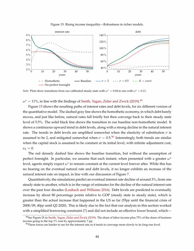
Figure 15: Rising income inequality—Robustness in richer models.

0 10 20 30 40 502 %

3 %

4 %

5 %

6 %

7 %

8 %

9 %

years

interest rate

0 10 20 30 40 5040 %

60 %

80 %

100 %

120 %

140 %

years

debt

Homothetic Baseline σ = 2 σ = 0.5 K = constNo perfect foresight

Note. Plots show transitions from our calibrated steady state with ωs = 0.04 to one with ωs = 0.11.

ωs = 11%, in line with the findings of Smith, Yagan, Zidar and Zwick (2019).49

Figure 15 shows the resulting paths of interest rates and debt levels, for six different version ofthe quantitative model. The dashed gray line shows the homothetic economy, in which debt barelymoves, and just like before, natural rates fall briefly but then converge back to their steady statelevel of 5.5%. The solid black line shows the transition in our baseline non-homothetic model. Itshows a continuous upward trend in debt levels, along with a strong decline in the natural interestrate. The trends in debt levels are amplified somewhat when the elasticity of substitution σ isassumed to be 2, and mitigated somewhat when σ = 0.5.50 Interestingly, both trends are similarwhen the capital stock is assumed to be constant at its initial level, with infinite adjustment cost,εK = 0.

The red densely dashed line shows the baseline transition, but without the assumption ofperfect foresight. In particular, we assume that each instant, when presented with a greater ωs

level, agents simply expect ωs to remain constant at the current level forever after. While this hasno bearing on the eventual natural rate and debt levels, it no longer exhibits an increase of thenatural interest rate on impact, in line with our discussion of Figure 7.

Quantitatively, the simulations predict an eventual interest rate decline of around 3%, from onesteady state to another, which is in the range of estimates for the decline of the natural interest rateover the past four decades (Laubach and Williams 2016). Debt levels are predicted to eventuallyincrease by about 80 percentage points relative to GDP (steady state to steady state), which isgreater than the actual increase that happened in the US so far (55pp until the financial crisis of2008/09, 40pp until Q2 2020). This is likely due to the fact that our analysis in this section workedwith a simplified borrowing constraint (7) and did not include an effective lower bound, which—

49See Figure IX in Smith, Yagan, Zidar and Zwick (2019). The share of labor income plus 75% of the share of businessincome going to the top 1% rose by approximately 7 pp.

50These forces are harder to see for the interest rate as it tends to converge more slowly to its long-run level.

44

as shown in Figure 13—mitigates the increase in debt levels.

X Conclusion

In this paper, we proposed a new theory connecting several recent secular trends: the increase inincome inequality, financial deregulation, the decline in natural interest rates, and the rise in debtby households and governments.

The central element in our theory are non-homothetic preferences, which lead richer house-holds to have greater saving rates out of a permanent income transfer. This gives rise to the ideaof indebted demand: greater debt levels mean a greater transfer of income in the form of debtservice payments from borrowers to savers, and thus depress demand.

We identified three main implications of indebted demand. First, secular economic shifts thatraise debt levels (e.g. income inequality or financial deregulation) also lower natural interest rates,which then itself has an amplified effect on debt. Second, monetary and fiscal policy, to the extentthat they involve household or government debt creation, can persistently reduce future naturalinterest rates. This means that there is only a limited number of such policy interventions thatcan be used before economies approach the effective lower bound. Finally, when the lower boundis binding, the economy is in a liquidity trap with depressed output. In this “debt trap”, debt-financed stimulus deepens the recession in the future, whereas redistributive policies and policiesaddressing the structural sources of inequality mitigate it.

Our results suggest that economies face a sort of “budget constraint for aggregate demand”.They can stimulate aggregate demand through debt creation, but that reduces future demand (andthus natural interest rates). This logic suggests a new trade-off for debt-based stimulus policies.We view an exploration of this trade-off in an optimal policy setting as a promising avenue forfuture research.

PRINCETON AND NATIONAL BUREAU OF ECONOMIC RESEARCHHARVARD AND NATIONAL BUREAU OF ECONOMIC RESEARCHCHICAGO BOOTH AND NATIONAL BUREAU OF ECONOMIC RESEARCH

45

References

Aiyagari, S Rao. 1994. “Uninsured idiosyncratic risk and aggregate saving.” The Quarterly Journal of Eco-nomics, 109(3): 659–684.

Aiyagari, S. Rao, and Ellen McGrattan. 1998. “The optimum quantity of debt.” Journal of Monetary Eco-nomics, 42(3): 447–469.

Arrondel, Luc, Pierre Lamarche, and Frederique Savignac. 2019. “Does inequality matter for theconsumption-wealth channel? Empirical evidence.” European Economic Review, 111: 139–165.

Atkinson, Anthony B, Thomas Piketty, and Emmanuel Saez. 2011. “Top incomes in the long run of his-tory.” Journal of Economic Literature, 49(1): 3–71.

Auclert, Adrien, and Matthew Rognlie. 2018. “Inequality and Aggregate Demand.” National Bureau ofEconomic Research Working Paper 24280.

Auclert, Adrien, Matthew Rognlie, and Ludwig Straub. 2018. “The Intertemporal Keynesian Cross.” Na-tional Bureau of Economic Research Working Paper 25020.

Auclert, Adrien, Matthew Rognlie, and Ludwig Straub. 2020. “Micro Jumps, Macro Humps: MonetaryPolicy and Business Cycles in an Estimated HANK Model.” National Bureau of Economic ResearchWorking Paper 26647.

Autor, David, Frank Levy, and Richard J. Murnane. n.d.. “The Skill Content of Recent TechnologicalChange: An Empirical Exploration.” The Quarterly Journal of Economics, 118(4): 1279–1333.

Ball, Michael. 1990. Under one roof: retail banking and the international mortgage finance revolution. HarvesterWheatsheaf.

Bartscher, Alina K, Moritz Kuhn, Moritz Schularick, and Ulrike Steins. 2020. “Modigliani Meets Minsky:Inequality, Debt, and Financial Fragility in America, 1950-2016.”

Benhabib, Jess, Alberto Bisin, and Mi Luo. 2019. “Wealth distribution and social mobility in the US: Aquantitative approach.” American Economic Review, 109: 1623–47.

Benigno, Gianluca, and Luca Fornaro. 2018. “Stagnation traps.” The Review of Economic Studies, 85(3): 1425–1470.

Beraja, Martin, Andreas Fuster, Erik Hurst, and Joseph Vavra. 2018. “Regional Heterogeneity and theRefinancing Channel of Monetary Policy.” The Quarterly Journal of Economics, 134(1): 109–183.

Berger, David W, Konstantin Milbradt, Fabrice Tourre, and Joseph Vavra. 2018. “Mortgage Prepaymentand Path-Dependent Effects of Monetary Policy.” National Bureau of Economic Research Working Paper25157.

Bernanke, Ben S. 2005. “The global saving glut and the U.S. current account deficit.” Board of Governorsof the Federal Reserve System (U.S.) Speech 77.

Bernanke, Ben S, and Mark Gertler. 2001. “Should central banks respond to movements in asset prices?”American Economic Review, 91(2): 253–257.

Bhutta, Neil, and Benjamin J. Keys. 2016. “Interest Rates and Equity Extraction during the HousingBoom.” American Economic Review, 106(7): 1742–74.

Blanchard, Olivier. 1985. “Debt, Deficits, and Finite Horizons.” Journal of Political Economy, 93(2): 223–247.

Bokhari, Sheharyar, Walter Torous, and William Wheaton. 2013. “Why did household mortgage leveragerise from the mid-1980s until the great recession.” Citeseer.

46

Borio, Claudio, and Piti Disyatat. 2014. “Low interest rates and secular stagnation: is debt a missing link?”VoxEU.

Borio, Claudio, and William White. 2004. “Whither monetary and financial stability? the implications ofevolving policy regimes.” BIS Working Papers.

Bourguignon, Francois. 1981. “Pareto superiority of unegalitarian equilibria in Stiglitz’model of wealthdistribution with convex saving function.” Econometrica: Journal of the Econometric Society, 1469–1475.

Caballero, Ricardo, and Emmanuel Farhi. 2017. “The safety trap.” The Review of Economic Studies,85(1): 223–274.

Caballero, Ricardo J, and Alp Simsek. 2019. “Prudential Monetary Policy.” National Bureau of EconomicResearch Working Paper 25977.

Caballero, Ricardo J, Emmanuel Farhi, and Pierre-Olivier Gourinchas. 2017. “The safe assets shortageconundrum.” Journal of Economic Perspectives, 31(3): 29–46.

Cairo, Isabel, and Jae W. Sim. 2018. “Income Inequality, Financial Crises, and Monetary Policy.” Board ofGovernors of the Federal Reserve System (U.S.) Finance and Economics Discussion Series 2018-048.

Calza, Alessandro, Tommaso Monacelli, and Livio Stracca. 2013. “Housing Finance and Monetary Policy.”Journal of the European Economic Association, 11(S1): 101–122.

Campbell, John Y. 2013. “Mortgage Market Design.” Review of Finance, 17(1): 1–33.

Campbell, John Y, Nuno Clara, and Joao F Cocco. 2020. “Structuring Mortgages for Macroeconomic Sta-bility.” National Bureau of Economic Research Working Paper 27676.

Carroll, Christopher. 2000. “Why Do the Rich Save So Much?”

Chodorow-Reich, Gabriel, Plamen T Nenov, and Alp Simsek. 2019. “Stock Market Wealth and the RealEconomy: A Local Labor Market Approach.” National Bureau of Economic Research Working Paper25959.

Cloyne, James, Clodomiro Ferreira, and Paolo Surico. 2019. “Monetary Policy when Households haveDebt: New Evidence on the Transmission Mechanism.” The Review of Economic Studies, 87(1): 102–129.

Coeurdacier, Nicolas, Stephane Guibaud, and Keyu Jin. 2015. “Credit Constraints and Growth in a GlobalEconomy.” American Economic Review, 105(9): 2838–81.

Cole, Harold L, George J Mailath, and Andrew Postlewaite. 1992. “Social norms, savings behavior, andgrowth.” Journal of Political economy, 100(6): 1092–1125.

Corneo, Giacomo, and Olivier Jeanne. 1997. “On relative wealth effects and the optimality of growth.”Economics letters, 54(1): 87–92.

Dalio, Ray. 2018. Principles For Navigating Big Debt Crises. Bridgewater.

De Nardi, Mariacristina. 2004. “Wealth inequality and intergenerational links.” The Review of EconomicStudies, 71(3): 743–768.

De Nardi, Mariacristina, Eric French, John Bailey Jones, and Angshuman Gooptu. 2011. “Medicaid andthe Elderly.” National Bureau of Economic Research Working Paper 17689.

Di Maggio, Marco, Amir Kermani, and Christopher J Palmer. 2020. “How quantitative easing works:Evidence on the refinancing channel.” The Review of Economic Studies, 87(3): 1498–1528.

47

Di Maggio, Marco, Amir Kermani, Benjamin J. Keys, Tomasz Piskorski, Rodney Ramcharan, Amit Seru,and Vincent Yao. 2017. “Interest Rate Pass-Through: Mortgage Rates, Household Consumption, andVoluntary Deleveraging.” American Economic Review, 107(11): 3550–88.

Drehmann, Mathias, Mikael Juselius, and Anton Korinek. 2018. “Going With the Flows: New Borrowing,Debt Service and the Transmission of Credit Booms.” National Bureau of Economic Research WorkingPaper 24549.

Dynan, Karen E., Jonathan Skinner, and Stephen P. Zeldes. 2004. “Do the Rich Save More?” Journal ofPolitical Economy, 112(2): 397–444.

Eggertsson, Gauti B., and Paul Krugman. 2012. “Debt, Deleveraging, and the Liquidity Trap: A Fisher-Minsky-Koo Approach.” Quarterly Journal of Economics, 127(3): 1469–1513.

Eggertsson, Gauti B, Jacob A Robbins, and Ella Getz Wold. 2018. “Kaldor and Piketty’s Facts: The Rise ofMonopoly Power in the United States.” National Bureau of Economic Research Working Paper 24287.

Eggertsson, Gauti B., Neil R. Mehrotra, and Jacob A. Robbins. 2019. “A Model of Secular Stagnation:Theory and Quantitative Evaluation.” American Economic Journal: Macroeconomics, 11(1): 1–48.

Eichenbaum, Martin, Sergio Rebelo, and Arlene Wong. 2019. “State Dependent Effects of Monetary Pol-icy: the Refinancing Channel.” Working Paper.

Fagereng, Andreas, Martin Blomhoff Holm, Benjamin Moll, and Gisle Natvik. 2019. “Saving BehaviorAcross the Wealth Distribution: The Importance of Capital Gains.” National Bureau of Economic Re-search Working Paper 26588.

Farhi, Emmanuel, and Francois Gourio. 2018. “Accounting for Macro-Finance Trends: Market Power, In-tangibles, and Risk Premia.” Brookings Papers on Economic Activity, Fall: 147–250.

Farhi, Emmanuel, and Ivan Werning. 2016. “A theory of macroprudential policies in the presence of nom-inal rigidities.” Econometrica, 84(5): 1645–1704.

Favilukis, Jack, Sydney C Ludvigson, and Stijn Van Nieuwerburgh. 2017. “The macroeconomic effectsof housing wealth, housing finance, and limited risk sharing in general equilibrium.” Journal of PoliticalEconomy, 125(1): 140–223.

Fisher, Jonathan, David Johnson, Timothy Smeeding, and Jeffrey Thompson. 2018. “Inequality in 3-D:Income, Consumption, and Wealth.” Board of Governors of the Federal Reserve System Finance and EconomicsDiscussion Series 2018-001.

Garbinti, Bertrand, Pierre Lamarche, Charlelie Lecanu, and Frederique Savignac. 2020. “Wealth effect onconsumption during the sovereign debt crisis: Households heterogeneity in the Euro area.” ECB WorkingPaper 2357.

Greenwald, Daniel. 2018. “The mortgage credit channel of macroeconomic transmission.” MIT Sloan Re-search Paper.

Guerrieri, Veronica, and Guido Lorenzoni. 2017. “Credit crises, precautionary savings, and the liquiditytrap.” The Quarterly Journal of Economics, 132(3): 1427–1467.

Guren, Adam M, Arvind Krishnamurthy, and Timothy J McQuade. 2021. “Mortgage design in an equi-librium model of the housing market.” The Journal of Finance, 76(1): 113–168.

Gutierrez, German, and Thomas Philippon. 2016. “Investment-less Growth: An Empirical Investigation.”National Bureau of Economic Research Working Paper 22897.

Guvenen, Fatih, Greg Kaplan, Jae Song, and Justin Weidner. 2017. “Lifetime Incomes in the United Statesover Six Decades.” National Bureau of Economic Research Working Paper 23371.

48

Guvenen, Fatih, Gueorgui Kambourov, Burhanettin Kuruscu, Sergio Ocampo-Diaz, and Daphne Chen.2019. “Use It or Lose It: Efficiency Gains from Wealth Taxation.” National Bureau of Economic ResearchWorking Paper 26284.

Hayashi, Fumio. 1982. “Tobin’s marginal q and average q: A neoclassical interpretation.” Econometrica:Journal of the Econometric Society, 213–224.

Iachan, Felipe S, Plamen T Nenov, and Alp Simsek. 2015. “The Choice Channel of Financial Innovation.”National Bureau of Economic Research Working Paper 21686.

Illing, Gerhard, Yoshiyasu Ono, and Matthias Schlegl. 2018. “Credit booms, debt overhang and secularstagnation.” European Economic Review, 78(104).

Jorda, Oscar, Moritz Schularick, and Alan M Taylor. 2016. “The great mortgaging: housing finance, crisesand business cycles.” Economic Policy, 31(85): 107–152.

Justiniano, Alejandro, Giorgio E Primiceri, and Andrea Tambalotti. 2017. “The Mortgage Rate Conun-drum.” National Bureau of Economic Research Working Paper 23784.

Kaplan, Greg, Kurt Mitman, and Giovanni L Violante. 2020. “The housing boom and bust: Model meetsevidence.” Journal of Political Economy, 128(9): 3285–3345.

Katz, Lawrence F, and Kevin M Murphy. 1992. “Changes in relative wages, 1963–1987: supply and demandfactors.” The Quarterly Journal of Economics, 107(1): 35–78.

Koopmans, Tjalling C. 1960. “Stationary ordinal utility and impatience.” Econometrica: Journal of the Econo-metric Society, 287–309.

Koo, Richard. 2008. The Holy Grail of Macroeconomics - Lessons from Japan’s Great Recession. Wiley.

Kopczuk, Wojciech, Emmanuel Saez, and Jae Song. 2010. “Earnings inequality and mobility in the UnitedStates: evidence from social security data since 1937.” The Quarterly Journal of Economics, 125(1): 91–128.

Korinek, Anton, and Alp Simsek. 2016. “Liquidity trap and excessive leverage.” American Economic Review,106(3): 699–738.

Krusell, Per, Lee E. Ohanian, Jose-Victor Rios-Rull, and Giovanni L. Violante. 2000. “Capital-Skill Com-plementarity and Inequality: A Macroeconomic Analysis.” Econometrica, 68(5): 1029–1053.

Kumhof, Michael, Romain Ranciere, and Pablo Winant. 2015. “Inequality, leverage, and crises.” AmericanEconomic Review, 105(3): 1217–45.

Laubach, Thomas, and John C Williams. 2016. “Measuring the natural rate of interest redux.” BusinessEconomics, 51(2): 57–67.

Liu, Ernest, Atif Mian, and Amir Sufi. 2019. “Low Interest Rates, Market Power, and Productivity Growth.”National Bureau of Economic Research Working Paper 25505.

Lo, Stephanie, and Kenneth S. Rogoff. 2015. “Secular stagnation, debt overhang and other rationales forsluggish growth, six years on.” Bank for International Settlements BIS Working Papers 482.

McKay, Alisdair, and Johannes F Wieland. 2019. “Lumpy Durable Consumption Demand and the LimitedAmmunition of Monetary Policy.” National Bureau of Economic Research Working Paper 26175.

McKay, Alisdair, Emi Nakamura, and Jon Steinsson. 2016. “The Power of Forward Guidance Revisited.”American Economic Review, 106(10): 3133–3158.

Mian, Atif, Amir Sufi, and Emil Verner. 2017. “Household debt and business cycles worldwide.” TheQuarterly Journal of Economics, 132(4): 1755–1817.

49

Mian, Atif, and Amir Sufi. 2015. House of debt: How they (and you) caused the Great Recession, and how we canprevent it from happening again. University of Chicago Press.

Mian, Atif R, Ludwig Straub, and Amir Sufi. 2020. “The Saving Glut of the Rich and the Rise in HouseholdDebt.” National Bureau of Economic Research Working Paper 26941.

Michaillat, Pascal, and Emmanuel Saez. 2019. “Resolving New Keynesian anomalies with wealth in theutility function.” Review of Economics and Statistics, 1–46.

Michau, Jean-Baptiste. 2018. “Secular stagnation: Theory and remedies.” Journal of Economic Theory,176: 552–618.

Ono, Yoshiyasu. 1994. Money, interest, and stagnation: Dynamic theory and Keynes’s economics. Oxford Univer-sity Press.

Pettis, Michael. 2019. “Wealth Should Trickle Up, Not Down.” Carnegie Endowment for InternationalPeace Washington DC.

Piketty, Thomas. 2014. Capital in the Twenty-First Century. Belknap Press: An Imprint of Harvard UniversityPress.

Piketty, Thomas, and Emmanuel Saez. 2003. “Income Inequality in the United States, 1913-1998.” QuarterlyJournal of Economics, 118(1): 1–41.

Piketty, Thomas, Emmanuel Saez, and Gabriel Zucman. 2017. “Distributional national accounts: methodsand estimates for the United States.” The Quarterly Journal of Economics, 133(2): 553–609.

Rachel, Lukasz, and Lawrence H Summers. 2019. “On falling neutral real rates, fiscal policy and the riskof secular stagnation.” Brookings Papers on Economic Activity BPEA Conference Drafts, March 7-8.

Rannenberg, Ansgar. 2019. “Inequality, the risk of secular stagnation and the increase in household debt.”NBB Working Paper 375, Brussels:National Bank of Belgium.

Ravn, Morten O, and Vincent Sterk. 2020. “Macroeconomic Fluctuations with HANK + SAM: an AnalyticalApproach.” Journal of the European Economic Association.

Reinhart, Carmen M., and Kenneth S. Rogoff. 2009. This Time is Different: Eigth Centuries of Financial Folly.Princeton University Press.

Reinhart, Carmen M, and Kenneth S Rogoff. 2010. “Growth in a Time of Debt.” American economic review,100(2): 573–78.

Romer, Christina D, and David H Romer. 2004. “A new measure of monetary shocks: Derivation andimplications.” American Economic Review, 94(4): 1055–1084.

Saez, Emmanuel, and Gabriel Zucman. 2019. “Progressive wealth taxation.” Brookings Papers on EconomicActivity, 2019(2): 437–533.

Saez, Emmanuel, and Gabriel Zucman. 2020. “Trends in US Income and Wealth Inequality: Revising Afterthe Revisionists.” National Bureau of Economic Research Working Paper 27921.

Saez, Emmanuel, and Stefanie Stantcheva. 2018. “A simpler theory of optimal capital taxation.” Journal ofPublic Economics, 162: 120–142.

Sarin, Natasha, Lawrence Summers, and Joe Kupferberg. 2020. “Tax Reform for Progressivity: A Prag-matic Approach.” Tackling the Tax Code: Efficient and Equitable Ways to Raise Revenue.

Schularick, Moritz, and Alan M Taylor. 2012. “Credit booms gone bust: Monetary policy, leverage cycles,and financial crises, 1870-2008.” American Economic Review, 102(2): 1029–61.

50

Smith, Matthew, Danny Yagan, Owen Zidar, and Eric Zwick. 2019. “Capitalists in the Twenty-first Cen-tury.” The Quarterly Journal of Economics, 134(4): 1675–1745.

Stein, Jeremy C. 2012. “Monetary Policy as Financial-Stability Regulation.” Quarterly Journal of Economics,127(1): 57–95. Draft Date: Revised May 2011.

Stein, Jeremy C. 2013. “Overheating in Credit Markets: Origins, Measurement, and Policy Responses.”Speech at Federal Reserve Bank of St Louis.

Stiglitz, Joseph E. 1969. “Distribution of income and wealth among individuals.” Econometrica: Journal ofthe Econometric Society, 382–397.

Straub, Ludwig. 2019. “Consumption, Savings, and the Distribution of Permanent Income.”

Strotz, Robert Henry. 1956. “Myopia and inconsistency in dynamic utility maximization.” The Review ofEconomic Studies, 23(3): 165–180.

Summers, Lawrence H. 2014. “US economic prospects: Secular stagnation, hysteresis, and the zero lowerbound.” Business Economics, 49(2): 65–73.

Summers, Lawrence H. 2015. “Demand side secular stagnation.” American Economic Review, 105(5): 60–65.

Svensson, Lars E. O. 2018. “Monetary policy and macroprudential policy: Different and separate?” Cana-dian Journal of Economics, 51(3): 802–827.

Turner, Adair. 2015. Between Debt and the Devil: Money, Credit, and Fixing Global Finance. Princeton UniversityPress.

Uzawa, Hirofumi. 1968. “Market allocation and optimum growth.” Australian Economic Papers, 7(10): 17–27.

Von Schlicht, Ekkehart. 1975. “A neoclassical theory of wealth distribution.” Jahrbucher fur Nationalokonomieund Statistik, 189(1-2): 78–96.

Werning, Ivan. 2015. “Incomplete Markets and Aggregate Demand.” National Bureau of Economic Re-search Working Paper 21448.

51