NBER WORKING PAPER SERIES

INDEBTED DEMAND

Atif R. MianLudwig Straub

Amir Sufi

Working Paper 26940http://www.nber.org/papers/w26940

NATIONAL BUREAU OF ECONOMIC RESEARCH1050 Massachusetts Avenue

Cambridge, MA 02138April 2020

We thank George-Marios Angeletos, Heather Boushey, Fatih Guvenen, Gerhard Illing, Ernest Liu, Fabrizio Perri, Andrei Shleifer, Alp Simsek, Jeremy Stein, Larry Summers, and Ivan Werning as well as seminar participants at Harvard, Princeton, Chicago Booth, Stanford, UCLA, Bocconi, LMU, ECB, and Banque de France for numerous useful comments. Sebastian Hanson, Bianca He, Julio Roll, and Ian Sapollnik provided excellent research assistance. Straub appreciates support from the Molly and Domenic Ferrante Award. Contact info: Mian: (609) 258 6718, atif@princeton.edu; Straub: (617) 496 9188, ludwigstraub@fas.harvard.edu; Sufi: (773) 702 6148, amir.sufi@chicagobooth.edu. The views expressed herein are those of the authors and do not necessarily reflect the views of the National Bureau of Economic Research.

NBER working papers are circulated for discussion and comment purposes. They have not been peer-reviewed or been subject to the review by the NBER Board of Directors that accompanies official NBER publications.

© 2020 by Atif R. Mian, Ludwig Straub, and Amir Sufi. All rights reserved. Short sections of text, not to exceed two paragraphs, may be quoted without explicit permission provided that full credit, including © notice, is given to the source.

Indebted DemandAtif R. Mian, Ludwig Straub, and Amir SufiNBER Working Paper No. 26940April 2020JEL No. D31,E21,E32,E43,E44,E52,E62,G51

ABSTRACT

We propose a theory of indebted demand, capturing the idea that large debt burdens by households and governments lower aggregate demand, and thus natural interest rates. At the core of the theory is the simple yet under-appreciated observation that borrowers and savers differ in their marginal propensities to save out of permanent income. Embedding this insight in a two-agent overlapping-generations model, we find that recent trends in income inequality and financial liberalization lead to indebted household demand, pushing down natural interest rates. Moreover, popular expansionary policies—such as accommodative monetary policy and deficit spending—generate a debt-financed short-run boom at the expense of indebted demand in the future. When demand is sufficiently indebted, the economy gets stuck in a debt-driven liquidity trap, or debt trap. Escaping a debt trap requires consideration of less standard macroeconomic policies, such as those focused on redistribution or those reducing the structural sources of high inequality.

Atif R. MianPrinceton UniversityBendheim Center For Finance26 Prospect AvenuePrinceton, NJ 08540and NBERatif@princeton.edu

Ludwig StraubDepartment of EconomicsHarvard UniversityLittauer 211Cambridge, MA 02139and NBERludwigstraub@fas.harvard.edu

Amir SufiUniversity of ChicagoBooth School of Business5807 South Woodlawn AvenueChicago, IL 60637and NBERamir.sufi@chicagobooth.edu

1 Introduction

Rising debt and falling interest rates have characterized advanced economies over the past 40years. The average real interest rate dropped from 6% in 1980 to less than zero in 2019 (Racheland Summers 2019), and the average debt to GDP ratio almost doubled from 139% in 1980 to over270% (Figure 1 below). The economic fallout of the COVID-19 health crisis is likely to acceleratethese patterns going forward, as governments pursue aggressive debt-financed stimulus policies.

This situation raises critical research questions: How did the twin phenomena of high debt lev-els and low interest rates come to be? Should there be a reconsideration of the standard macroeco-nomic toolkit of monetary and fiscal policy given the challenging environment of high debt levelsand low interest rates? Is there a more prominent role for policies focused on redistribution?

This study develops a new framework to tackle these difficult questions. The frameworkshows how rising income inequality and the liberalization of the financial sector can push economiesinto a low interest rate-high debt environment. Traditional macroeconomic policies such as mon-etary and fiscal policy turn out to be less effective over the long term in such an environment. Onthe other hand, less standard policies such as macro-prudential regulation, redistribution policy,and policies addressing the structural sources of high inequality are more powerful and long-lasting.

The model introduces non-homothetic consumption-saving behavior (e.g. Carroll 2000, De Nardi2004, Straub 2019) into an otherwise conventional, deterministic two-agent endowment economy.The assumption of non-homotheticity implies that the saver in the model saves a larger fraction oflifetime income than the borrower. This is not a new idea in economics. In fact, it is pervasive inthe work of luminaries such as John Atkinson Hobson, Eugen von Bohm-Bawerk, Irving Fisher,and John Maynard Keynes, and empirically supported by recent work (e.g., Dynan, Skinner, andZeldes 2004, Straub 2019, and Fagereng, Holm, Moll, and Natvik 2019). In the model, the wealthylend to the rest of the population, which makes household debt an important financial asset in theportfolio of the wealthy.1

The assumption of non-homotheticity in our model generates the crucial property that largedebt levels weigh negatively on aggregate demand: as borrowers reduce their spending to makedebt payments to savers, the latter, having greater saving rates, only imperfectly offset the shortfallin borrowers’ spending. We refer to a situation in which demand is depressed due to elevated debtlevels as indebted demand.

The concept of indebted demand has broad implications for understanding what has led tothe current high debt and low interest rate environment, and for evaluating what policies canpotentially help advanced economies escape this equilibrium. An overarching theme of the modelis that shifts or policies that boost demand today through debt accumulation necessarily reducedemand going forward by shifting resources from borrowers to savers; therefore, such shifts orpolicies actually contribute to persistently low interest rates.

1This implication of the model fits the data, as shown in Mian, Straub, and Sufi (2019); a substantial fraction ofhousehold debt in the United States reflects the top 10% of the wealth distribution lending to the bottom 90%.

2

The indebted demand framework predicts a number of patterns found in the data that modelswithout non-homotheticity in the consumption-saving behavior of agents have a difficult timeexplaining. For example, since the 1980s, many advanced economies have experienced a largerise in top income shares (Katz and Murphy 1992, Piketty and Saez 2003, Piketty 2014, Piketty,Saez, and Zucman 2017), in conjunction with a substantial decline in interest rates and increasesin household and government debt. The model predicts exactly such an outcome: a rise in topincome shares in the model shifts resources from borrowers to savers, pushing down interest ratesdue to savers’ greater desire to save. Lower interest rates stimulate more debt, causing indebteddemand—as debt is nothing other than an additional shift of resources in the form of debt servicepayments from borrowers to savers.

The framework also predicts that financial liberalization, which has been a prominent featureof advanced economies since the 1980s, leads to a decline in interest rates, a result that is difficult togenerate in most macroeconomic models (e.g., Justiniano, Primiceri, and Tambalotti 2017). In theindebted demand model, financial liberalization increases the amount of debt taken on by borrow-ers, which redistributes resources to savers. For the goods markets to clear, such a redistributionrequires interest rates to fall given that savers have a lower marginal propensity to consume outof these larger debt payments.

More generally, the model offers a different perspective on the growth in the size of the finan-cial sector since the 1980s. Traditional models in which the financial sector enables firms to borrowfrom households cannot explain the global rise in debt to GDP ratios, which has been concentratedin household and government debt. Furthermore, investment to GDP ratios and business produc-tivity growth have actually fallen during this period. In contrast, the indebted demand modelfocuses on how secular forces such as rising inequality and financial liberalization can foster alarge rise in households borrowing from other households. In both the model and the data, thehousehold sector is crucial for understanding why debt levels have increased.

The concept of indebted demand also provides insight into discussions of monetary and fiscalpolicy. For example, deficit-financed fiscal policy in the model is associated with a short run risein natural interest rates, which reverses into a reduction in interest rates in the long-run, as thegovernment needs to raise taxes or cut spending in order to finance the greater government debtburden.2 As long as some of the taxes are ultimately imposed on borrowers, deficit-financed gov-ernment spending is similar to any policy which attempts to boost demand through debt accumu-lation. Ultimately, such a policy shifts resources from borrowers to savers, depressing aggregatedemand and therefore interest rates in the long run.

A similar argument applies to monetary policy, for which we extend our model to includenominal rigidities. Empirical evidence suggests that an important channel of accommodativemonetary policy operates through an increase in debt accumulation (e.g., Bhutta and Keys 2016,Di Maggio, Kermani, Keys, Piskorski, Ramcharan, Seru, and Yao 2017, Beraja, Fuster, Hurst, and

2As we discuss below, we find that a similar result holds up in the presence of spreads between government bondyields and the returns on other assets.

3

Vavra 2018, Di Maggio, Kermani, and Palmer 2019, Cloyne, Ferreira, and Surico 2019). This chan-nel is also active in our model, boosting demand in the short-run. However, this boost reverses asmonetary stimulus fades and debt needs to be serviced, beginning to drag on demand. Due to thepresence of indebted demand, this drag can cause a persistent shift in natural interest rates aftertemporary monetary policy interventions. It is for this reason that monetary policy has limitedammunition in the model: successive monetary policy interventions build up debt levels, therebylowering natural rates. This forces policy rates to keep falling with them to avoid a recession, thusapproaching the effective lower bound.

When savers command sufficient resources in our economy, for instance due to high incomeinequality and large debt levels, the natural rate in our economy can be persistently below itseffective lower bound. At that point, our economy is in a debt-driven liquidity trap, or debt trap,which is a well-defined stable steady state of our economy.

The most striking aspect of this state is that it acts as a kind of “black hole”. Conventionalpolicies that are based on debt accumulation, such as deficit spending, only work in the shortrun. Eventually, the economy is “pulled back” into the debt trap. Certain unconventional policies,however, can facilitate an escape from the debt trap. For example, redistributive tax policies,such as wealth taxes, or structural policies that are geared towards reducing income inequalitygenerate a sustainable increase in demand, persistently raising natural interest rates away fromtheir effective lower bound. One-time debt forgiveness policies can also lift the economy out of thedebt trap, but need to be combined with other policies, such as macroprudential ones, to preventa return to the debt trap over time.

The idea of indebted demand helps explain the predicament faced by the world’s leadingcentral bankers, especially the absence of interest rate normalization. For example, a recent WallStreet Journal article cites monetary authorities worldwide in asserting that “borrowing helpedpull countries out of recession but made it harder for policy makers to raise rates.” Mark Carney,Governor of the Bank of England observed that “the sustainability of debt burdens depends oninterest rates remaining low.” Philip Lowe, Governor of the Reserve Bank of Australia has warnedthat “if interest rates were to rise . . . many consumers might have to severely curtail their spendingto keep up their repayments.”3 This paper formalizes these intuitions.

Literature. Our paper is part of a burgeoning literature on the causes of the recent fall in nat-ural interest rates, referred to as “secular stagnation” by Summers (2014). Among the existingexplanations are population aging (Eggertsson, Mehrotra, and Robbins 2019), income risk and in-come inequality (Auclert and Rognlie 2018, Straub 2019), the global saving glut (Bernanke 2005,Coeurdacier, Guibaud, and Jin 2015) and a shortage of safe assets (Caballero and Farhi 2017).4 Ourtheory suggests a new force for reduced natural interest rates, namely indebted demand. It can actboth as an amplifier of existing explanations—as we demonstrate for rising income inequality—or

3See also Borio and White (2004), Koo (2008), Borio and Disyatat (2014), Lo and Rogoff (2015), Turner (2015) andDalio (2018) for similar ideas.

4For an overview of multiple forces see Rachel and Summers (2019).

4

give rise to new explanations, as we demonstrate for financial liberalization, which is commonlythought to be a force against low interest rates.5

The central element of our theory is the assumption of non-homothetic preferences, generatingheterogeneous saving rates out of permanent income transfers.6 As we mentioned above, suchheterogeneity was an important aspect of many early studies of (non-optimizing) consumptionbehavior. Among the more recent papers in this tradition are Stiglitz (1969), Von Schlicht (1975),and Bourguignon (1981), who study the implications of such behavior on inequality. The earliestmodels of optimal consumption behavior that we know of and that allow for such preferencesare Strotz (1956), Koopmans (1960) and Uzawa (1968). More recently, Carroll (2000), De Nardi(2004), and Benhabib, Bisin, and Luo (2019) argue that non-homothetic preferences are importantto understand wealth inequality, and Straub (2019) studies their implications for a rise in incomeinequality.

Our implications for monetary policy are related to the debate around “leaning vs. cleaning”(Bernanke and Gertler 2001, Stein 2013, Svensson 2018) and to the nascent academic literaturesurrounding the idea that monetary policy might have limited ammunition. McKay and Wieland(2019) explore this idea in a model of durables spending, Caballero and Simsek (2019) in a modelwith asset price crashes.

The closest antecedents to our paper are Kumhof, Ranciere, and Winant (2015), Cairo and Sim(2018) and Rannenberg (2019). Kumhof, Ranciere, and Winant (2015) study a two-agent endow-ment economy, where savers are more patient than borrowers and savers have non-homotheticpreferences. They find that a rise in income inequality leads to greater debt levels and a greaterlikelihood of a financial crisis due to endogenous default, but no change in long-run interest rates.The driving force behind this result is the specific structure and heterogeneity of preferences. Itgenerates a higher saving rate of savers out of labor income, compared to borrowers, but a lowersaving rate out of financial income. This is why the model does not feature indebted demand: infact, an increase in debt raises aggregate demand in the model and thus dampens the effects ofincome inequality. The model in Cairo and Sim (2018) builds on Kumhof, Ranciere, and Winant(2015) and studies implications for a richer set of shocks and for the conduct of monetary pol-icy. The recent paper by Rannenberg (2019) also builds on Kumhof, Ranciere, and Winant (2015)but shows that income inequality can also reduce natural interest rates in addition to generatinggreater debt.

Finally, as a paper about household and government debt, it relates to a vast empirical andtheoretical literature on the origins and consequences of high debt levels. Among the empiricalpapers, Schularick and Taylor (2012) document the well known “financial hockey stick” behaviorof private debt; Mian and Sufi (2015), Jorda, Schularick, and Taylor (2016), Mian, Sufi, and Verner(2017) document that expansions in household debt predict weak future economic growth; Rein-hart and Rogoff (2010) assess the consequences of large government debt. Among the theoretical

5For a notable exception, see Iachan, Nenov, and Simsek (2015).6This is not to be confused with heterogeneity in marginal propensities to consume out of transitory income transfers,

which, as we explain below, are not sufficient to generate indebted demand.

5

papers, Eggertsson and Krugman (2012) and Guerrieri and Lorenzoni (2017) study the effects ofdebt deleveraging on the economy. Our model emphasizes that even without deleveraging, debtreduces aggregate demand. This aspect is shared with Illing, Ono, and Schlegl (2018), who showthat debt can lead to persistent stagnation in the context of insatiable preferences for money.

Layout. Section 2 presents motivating facts for our model, which we introduce in Section 3. Sec-tion 4 studies steady states and transitional dynamics in our model, introducing the concept ofindebted demand. In Section 5, we feed trends in income inequality and financial liberalizationinto the model. Next, we study the implications of fiscal policy (Section 6) and monetary policy(Section 7), and what indebted demand means for an economy in a liquidity trap (Section 8). Sec-tion 9 provides several extensions, and Section 10 offers a simple “sufficient statistic” perspectiveon our theory. Our conclusion is in Section 11.

2 Motivating Facts

2.1 High debt and low interest rates

A defining feature of advanced economies over the past decade has been the simultaneous pres-ence of historically high debt burdens and historically low interest rates. The massive debt-financed government fiscal programs being discussed in response to the COVID-19 health crisiswill likely accelerate this trend.

The left panel of Figure 1 plots the average debt to GDP ratio across 14 mostly advancedeconomies, where debt includes all borrowing by households, governments, and non-financialbusinesses. Both the high level of debt in recent years and its rapid ascent since 1980 are notable.

6

Figure 1: Debt and interest rates.

100

150

200

250

300T

ota

l C

red

it t

o G

DP

1950 1960 1970 1980 1990 2000 2010 2020

0

2

4

6

8

1970 1980 1990 2000 2010 2020

World real interest rate, King and Low, weighted by GDP

10 year treasury rate, US, real

30 year fixed mortgage rate, US, real

Left panel shows cross-country average total debt to GDP, weighted by real GDP in 1970. Total debt is the sum ofcredit to households, government and non-financial corporations. The countries in the sample are Australia, Canada,Finland, France, Germany, Italy, Japan, New Zealand, Norway, Portugal, Spain, Sweden, United States and UnitedKingdom. Data come from the IMF Global Debt Database, the Jorda-Schularick-Taylor Macrohistory Database and theNew Zealand Treasury. Right panel shows evolution of real interest rates. The real interest rate data start in the early1980s given that information on inflation expectations prior to 1980 is difficult to obtain. For more details on the datasources, see text.

The right panel shows the evolution of real interest rates from 1980 onward. The global interestrate is an estimate of the real rate of interest for 10-year inflation-protected government bonds fromKing and Low (2014). The right panel also shows the real interest rate on 10-year U.S. Treasuries,and an estimate of the real rate of interest for 30-year fixed rate mortgages in the United States.Measures of inflation expectations are taken from the Federal Reserve Bank of Cleveland (availablesince 1980). All three series show a substantial decline from 1980 onward.

7

Figure 2: Households and governments drove the increase in debt.

0

50

100

150

200

1950 1960 1970 1980 1990 2000 2010 2020

Corporate debt to GDP

Household & government debt to GDP

Series are cross-country average debt to GDP, for non-financial corporations and for households and governmentstogether, weighted by real GDP in 1970. The countries in the sample are Australia, Canada, Finland, France, Germany,Italy, Japan, New Zealand, Norway, Portugal, Spain, Sweden, United States and United Kingdom. Data come from theIMF Global Debt Database, the Jorda-Schularick-Taylor Macrohistory Database and the New Zealand Treasury.

Both the high level and rapid ascent of debt in advanced economies has been driven by bor-rowing by households and the government, as opposed to businesses. Figure 2 splits the totaldebt to GDP ratio into non-financial corporate debt and a second category that includes house-holds and governments, and it shows that the rise in debt has been concentrated in the lattercategory. Household and government debt to GDP ratios were relatively constant before 1980,before beginning an impressive upward trend through recent years. However, borrowing by thenon-financial corporate sector was modest, and therefore not responsible for the debt boom.

8

Figure 3: Secular decline of investment and TFP growth.

20

22

24

26

28A

vera

ge investm

en

t to

GD

P (

%)

1950 1960 1970 1980 1990 2000 2010 2020

−1

0

1

2

3

Avera

ge

TF

P g

row

th (

%)

1950 1960 1970 1980 1990 2000 2010 2020

Left panel shows cross-country average gross capital formation as a percentage of GDP and the right panel shows cross-country average total factor productivity growth, where the averages are weighted by real GDP in 1970. The countriesin the sample are Australia, Canada, Finland, France, Germany, Italy, Japan, New Zealand, Norway, Portugal, Spain,Sweden, United States and United Kingdom. Cross-country averages are constructed over 3-year moving averages atthe country-level. Data come from the Penn World Tables and World Bank World Development Indicators.

The fact that businesses have not been responsible for the rise in borrowing is consistent withthe fact that investment to GDP ratios have actually declined during this period of rising debt andlow interest rates. This is shown in the left panel of Figure 3, which plots the gross domestic invest-ment to GDP ratio across the 14 countries in the sample. The right panel shows that productivitygrowth has been at best constant (if not declining) over this time period.

The rise in debt has not been associated with a traditional channel through which businessesand the government borrow from the household sector to boost investment and productivitygrowth. Instead, rising debt levels appear to have been used to finance personal consumptionand government outlays. That is, it appears that the expansion of credit has been used to increaseaggregate demand rather than supply. This is a key motivating fact behind the model of indebteddemand below.

2.2 Inequality and household debt

The rising share of income earned by the top of the income distribution has been well-establishedin the literature (e.g., Piketty, Saez, and Zucman 2017). What is perhaps less well known is that therise in top income shares globally began in the 1980s at almost the exact same time as the rise ingovernment and household borrowing, and the two patterns have been closely linked afterward.This is shown in Figure 4, which plots the rise in government and household borrowing from Fig-ure 4 above, along with the top 1% share of income across 14 countries from the World Inequality

9

Database.

Figure 4: Rising inequality and rising debt.

8

10

12

14

16

Top 1

% incom

e s

hare

50

100

150

200

Household

& g

overn

ment debt to

GD

P (

%)

1950 1960 1970 1980 1990 2000 2010 2020

Household & government debt to GDP (%)

Top 1% income share

Series are cross-country averages, weighted by real GDP in 1970. The countries in the sample are Australia, Canada,Finland, France, Germany, Italy, Japan, New Zealand, Norway, Portugal, Spain, Sweden, United States and UnitedKingdom. Data come from the World Inequality Database, IMF Global Debt Database, the Jorda-Schularick-TaylorMacrohistory Database and the New Zealand Treasury.

This close association between the rise in inequality and the rise in household borrowing isexplored in detail in a companion study, Mian, Straub, and Sufi (2019). That study focuses on theUnited States, and it shows that the rise in income inequality has generated a “saving glut of therich,” which has financed a substantial rise in household debt by the non-rich.

One way to see this is Figure 5, which comes directly from Mian, Straub, and Sufi (2019). Itshows the stock of net household debt across the wealth distribution. Net household debt is de-fined as gross household debt owed minus household debt held as a financial asset. As the figureshows, the top 1% experienced a significant decline in their net debt position from 1982 onward,which reflects the accumulation of a significant amount of household debt held as a financial asset.In contrast, the bottom 90% experienced a large increase in their net debt position, as gross debtowed increased substantially but household debt held as a financial asset was relatively stable.Thus, to a large degree, the rise in saving of the top 1% has not been transformed into investmentor capital account surpluses; instead, it has been absorbed by an increase in borrowing by thebottom 90%.7

7As shown in Mian, Straub, and Sufi (2019), the evidence in Figure 5 is even stronger if saving and dissaving in otherassets, such as houses and the stock market, are included.

10

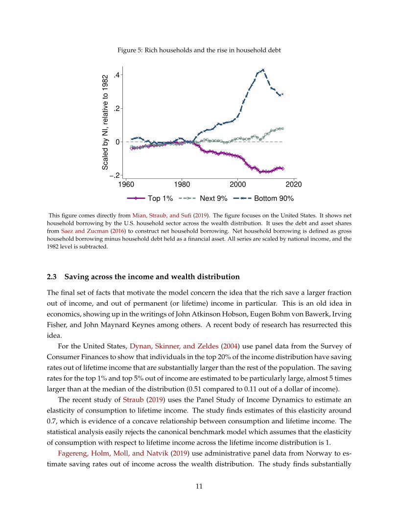
Figure 5: Rich households and the rise in household debt

−.2

0

.2

.4

Sca

led

by N

I, r

ela

tive

to

19

82

1960 1980 2000 2020

Top 1% Next 9% Bottom 90%

This figure comes directly from Mian, Straub, and Sufi (2019). The figure focuses on the United States. It shows nethousehold borrowing by the U.S. household sector across the wealth distribution. It uses the debt and asset sharesfrom Saez and Zucman (2016) to construct net household borrowing. Net household borrowing is defined as grosshousehold borrowing minus household debt held as a financial asset. All series are scaled by national income, and the1982 level is subtracted.

2.3 Saving across the income and wealth distribution

The final set of facts that motivate the model concern the idea that the rich save a larger fractionout of income, and out of permanent (or lifetime) income in particular. This is an old idea ineconomics, showing up in the writings of John Atkinson Hobson, Eugen Bohm von Bawerk, IrvingFisher, and John Maynard Keynes among others. A recent body of research has resurrected thisidea.

For the United States, Dynan, Skinner, and Zeldes (2004) use panel data from the Survey ofConsumer Finances to show that individuals in the top 20% of the income distribution have savingrates out of lifetime income that are substantially larger than the rest of the population. The savingrates for the top 1% and top 5% out of income are estimated to be particularly large, almost 5 timeslarger than at the median of the distribution (0.51 compared to 0.11 out of a dollar of income).

The recent study of Straub (2019) uses the Panel Study of Income Dynamics to estimate anelasticity of consumption to lifetime income. The study finds estimates of this elasticity around0.7, which is evidence of a concave relationship between consumption and lifetime income. Thestatistical analysis easily rejects the canonical benchmark model which assumes that the elasticityof consumption with respect to lifetime income across the lifetime income distribution is 1.

Fagereng, Holm, Moll, and Natvik (2019) use administrative panel data from Norway to es-timate saving rates out of income across the wealth distribution. The study finds substantially

11

higher saving rates for wealthier households, with saving rates for the top 1% estimated to bealmost double the saving rates for the median of wealth distribution.

Figure 6: Rising inequality and wealth accumulation across U.S. states

AL

AK

AZ

AR

CA

CO

CT

DE

DC FLGA

HI

ID

IL

IN

IA

KS

KYLA ME

MD

MA

MI MN

MS

MO

MT

NE

NV

NH

NJ

NM

NY

NC

ND

OH

OK

OR

PA

RI

SCSD

TN

TX

UT

VT

VA

WA

WV

WI

WY

−1

0

1

2

3

∆ W

ea

lth

to

In

co

me

.05 .1 .15 .2 .25

∆ Top 1% share

This figure plots the change from 1982 to 2007 in the ratio of total household wealth to household income at the statelevel against the change in the top 1% share of income over the same period. For full details on data, see Mian, Straub,and Sufi (2019).

These findings suggest that reallocation of resources from (income or wealth) non-rich house-holds to rich households increases aggregate saving. Mian, Straub, and Sufi (2019) provide ag-gregate evidence for this channel, based on heterogeneous trends in income inequality across U.S.states. In particular, as shown in Figure 6, states with larger increases in income inequality since1982 (as measured by their top 1% income shares) have significantly larger increases in accumu-lated wealth relative to average state-level income. While Figure 6 only displays a correlation,Mian, Straub, and Sufi (2019) show that this result is robust to variety of controls.

3 Model

Motivated by the facts above, this section develops a model of indebted demand. The modelis a deterministic, infinite-horizon endowment economy, populated by two separate dynasties ofagents trading debt contracts. Endowments can be thought of as dividends of real assets, or “Lucastrees”, owned by the two dynasties. Each such asset produces one unit of the consumption goodeach instant. There are Y real assets in total, where we normalize Y = 1 for now.

The agents in the two dynasties share the same preferences and only differ by their endow-ments of the real asset. For reasons that will become clear below, we refer to the poorer (“non-rich”) dynasty as borrowers i = b and wealthier (“rich”) dynasty as the savers i = s. At any point in

12

time, there is a mass µb = 1− µ of borrowers and a mass µs = µ of savers. We sometimes simplyrefer to all dynasties of type i as “agent” i.

The model is intentionally kept simple and tractable for now; several extensions can be foundin Section 9 and Appendix C.

3.1 Preferences

We begin by setting up the agents’ common preferences. An agent in dynasty i ∈ {b, s} dies atrate δ > 0 and discounts future utility at rate ρ > 0. At any date t, total consumption by dynastyi is ci

t and total wealth by dynasty i is ait. The average type-i agent therefore consumes ci

t/µi andowns wealth ai

t/µi, with a utility function given by8

∫ ∞

0e−(ρ+δ)t

{log(

cit/µi

)+

δ

ρv(ai

t/µi)

}dt (1)

Utility is derived from two components: each instant, utility over flow per-capita consumptionci

t/µi; and, arriving at rate δ, a warm-glow bequest motive captured by the function v(a)/ρ. Weassume for now that upon death, the entire asset position of an agent is bequeathed to a singlenewborn offspring, ruling out any cross-dynasty mobility.9 The consolidated budget constraint ofall agents of type i is therefore simply given by

cit + ai

t ≤ rtait (2)

where rt is the endogenous flow interest rate at date t.The function v(a) represents a crucial aspect of this model. It characterizes the relationship

between wealth of a dynasty and its saving rate. To see this, consider the special case wherev(a) = log a. This choice of v(a) makes the preferences in (1) homothetic: the borrower andsaver dynasties would exhibit the exact same saving behavior, just scaled by their current wealthpositions.10

This is no longer true as v(a) deviates from log a. To capture such deviations, we define ηi(a)to be the marginal utility of v relative to the marginal utility of log, that is,

ηi(a) ≡ a/µi · v′(a/µi). (3)

ηi(a) is defined in per-capita terms and therefore depends on i. ηi(a) plays an important role inthe analysis, especially ηs(a) which henceforth we also denote by η(a). When ηi(a) is constant,for instance ηi(a) = 1 when v(a) = log a, utility is homothetic as marginal utility of bequests andmarginal utility of consumption are proportional. When ηi(a) is decreasing, the marginal utility

8Our results also hold with non-unitary elasticities of the utility function over consumption, see Appendix C.1.9We relax this assumption in Section 9.4.

10In fact, given the normalization with 1/ρ, v(at) = log at exactly corresponds to an altruistic bequest motive in anequilibrium in which rt = ρ.

13

of bequeathing assets decreases relatively more quickly than the marginal utility of consumption;in this case, wealthier agents save relatively less. When ηi(a) is increasing, marginal bequest util-ity decays more slowly than that of consumption, implying that wealthier agents have a strongerdesire to save. This latter, non-homothetic case is the most plausible case intuitively and best sup-ported case empirically as mentioned in Section 2.3 above. This is the case focused on by themodel.

3.2 Borrowing constraint

The two types of agents in the model maximize utility (1) subject to the budget constraint (2) anda borrowing constraint. To formulate the borrowing constraint, we separate type-i agents’ wealthpositions into two components: their real assets hi

t and their financial assets, which if negative, werefer to as debt di

t, that is,ai

t = hit − di

t (4)

We assume for now that the agents’ debt is adjustable-rate long-term debt which decays at somerate λ > 0.

Agents of type i own a fixed total endowment of ωi ∈ (0, 1) of real assets (trees), where ωs +

ωb = 1. Within the endowment, we assume that `i < ωi are pledgeable real assets (e.g. land, houses,businesses, etc) and ωi − `i are non-pledgeable real assets (e.g. human capital). Denoting

pt ≡∫ ∞

te−∫ s

t ruduYds (5)

the price of a single real asset (tree), type-i agents’ total wealth in real assets is

hit = ptω

i (6)

and type-i agents’ pledgeable wealth is pt`i. Henceforth we assume that pledgeable wealth (percapita) is equal across agents, `b/(1 − µ) = `s/µ, and denote ` ≡ `b, so that the only sourceof heterogeneity between the two agents are the endowments ωi, or equivalently, the agents’real-asset earning shares. We assume that savers’ per capita earnings exceed those of borrowers,ωs/µs > ωb/µb.

We impose the borrowing constraint

dit + λdi

t ≤ λpt` (7)

where, due to asset market clearing, dst + db

t = 0.11 We henceforth focus exclusively on the borrow-ers’ total debt position dt ≡ db

t , the key state variable for our analysis. dt essentially captures howmuch borrowers have spent beyond earnings ωbY in the past, and how much of a debt burden

11We multiply the right hand side by λ so that in a steady state, the constraint simplifies to di ≤ p`. This is immaterialto our results.

14

borrowers need to service in the future.According to borrowing constraint (7), new debt issuance di + λdi

t is bounded above by thevalue of pledgeable assets. As we emphasize below, most of our results do not rely on the specificconstraint (7). In fact, we will often allow for a more general constraint of the form

dit + λdi

t ≤ λpt`({rs}s≥t) (8)

where ` = `({rs}s≥t) is a general function of current and future interest rates. With slight abuseof notation, we denote by `(r) the function `({rs}s≥t) in the case where rates are constant rs = rfor all s ≥ t. In Appendix C.2, we show that many alternative models of borrowing behaviorcan be expressed in this more general form. For example, in an economy with housing, `(r) ∝

r1+ϕr for some ϕ > 0. When borrowers are subject to uninsurable idiosyncratic income risk a laBewley-Aiyagari, we show that, under mild conditions, they endogenously choose an averagedebt position of the form p`(r) when rt = r in all periods. All examples share the characteristicthat the constraint on debt p`(r) is higher, i.e. more relaxed, for a lower interest rate r.

3.3 Homothetic benchmark

Throughout the analysis, we compare the model to a homothetic benchmark model. This model ischaracterized by η(a) = 1, so that agents’ preferences are indeed homothetic. Moreover, to avoid acontinuum of steady state equilibria in the homothetic model, we allow the saver’s discount factorto be different from, and smaller than, the borrower’s discount factor, ρs < ρ. Heterogeneity ofdiscount factors is not assumed in the non-homothetic model.

3.4 Equilibrium

We formally define equilibrium next.

Definition 1. Given initial debt d0 = db0 a (competitive) equilibrium of the model are sequences

{cit, ai

t, dit, hi

t, pt, rt} such that both agents choose {cit, ai

t} to maximize utility (1) subject to the budgetconstraint (2) and the borrowing constraint (7); di

t is determined by (4); hit is determined by (6); pt

is determined by (5); and financial markets clear at all times, that is, dst + db

t = 0. The goods marketclears by Walras’ law.

A steady state (equilibrium) is an equilibrium in which cit, ai

t, dit, hi

t and rt are all constant.A steady state with debt d is stable if there exists an ε > 0 such that any equilibrium with initial

debt d0 ∈ (d− ε, d + ε) has debt converge back to d, dt → d. All other steady states are unstable.

For illustrative purposes, we use the following parametrization of the non-homothetic andhomothetic models throughout the paper. We interpret the saver as comprising the top 1% earninghouseholds of the economy, i.e. with a population share µ = 0.01, and the borrower as the bottom99%. We choose the saver’s real (non-bond) earnings share ωs to match a pre-tax income shareof 20%. Subtracting the return to 150% household debt and government debt to GDP with a

15

4% interest rate, we arrive at ωs = 14%. The discount factor ρ will roughly correspond to theborrower’s discount factor and is set to a value of ρ = 0.10.

We directly calibrate η(a) = v′(a/µ)a/µ, letting it take the following simple functional form,η(a) = 1 + a−1 log

(1 + ea−a). From (3), this then determines v(a) and ηb(a). Given its functional

form, η(a) is strictly increasing with η′(a) ∈ (0, 1) and admits the homothetic model as a specialcase if a → ∞. The calibration uses the borrowing constraint (7). ` and a are jointly pinneddown to match a household-debt-to-GDP ratio of 80% and a steady-state interest rate r = 4%,which corresponds to the average real return on wealth.12 For the homothetic benchmark model,we achieve the interest rate target by assuming ρs = 0.04. The parameter λ has two roles. Itdetermines the maturity of debt, and it governs the speed of the debt response to relaxations inthe borrowing constraint. Until Section 9.6, we effectively assume the first role away by focusingexclusively on adjustable-rate debt, that is, debt has zero duration. Thus, we calibrate λ in linewith its second role. To do so, we compare the impulse response of household debt over GDP toa monetary policy shock implied by our model to that commonly found to identified monetarypolicy shocks. In particular, we feed a 4-year 50 basis points interest rate cut (see (17) below)into the Section 7 variant of our model and compare the household debt / GDP response at itspeak (after 2 years) with the year-2 response found in Jorda, Schularick, and Taylor (2015). Thisprocedure implies a λ roughly equal to 1. Finally, we set δ = 0.10. As we demonstrate in Section 10below, this produces a reasonable local slope of the saving supply curve of around dr/d log a ≈−0.032.

3.5 Discussion

What does η(a) capture? The literature has pointed out numerous examples of why agentsmight care about their wealth beyond its value for financing their own consumption behavior.This includes bequests (De Nardi 2004), out-of-pocket medical expenses in old age (De Nardi,French, Jones, and Gooptu 2011), utility over status (Cole, Mailath, and Postlewaite 1992), inter-vivos transfers (Straub 2019), and numerous other reasons that are documented in other papersin the literature (e.g. Carroll 2000, Dynan, Skinner, and Zeldes 2004, Saez and Stantcheva 2018,Boar 2018). Many of these examples are more salient or applicable to wealthier agents and can becaptured in reduced form by assuming a specific shape η(a). In addition to these examples, η(a)could also capture the idea that assets other than a given stock of liquid assets or human capitalare illiquid and therefore being saved “by holding” (Fagereng, Holm, Moll, and Natvik 2019).

Due to its stylized nature, our model is based entirely on bequests. We suspect microfoundedmodels of these other reasons for wealth accumulation among the rich behave similarly to ours.

Aggregate scale invariance. Our baseline non-homothetic model, with increasing η(a), is notscale-invariant in aggregate. If aggregate output Y doubles, all agents are wealthier and thus, in

12The correct analogue of r in the data is the real return on wealth, rather than the real safe rate. We present anextension in Section 9.3 that separates the two.

16

line with a rising η(a), would raise their savings by more than double. Taken at face value, thiswould generate rising saving rates in all growing economies, which seems counterfactual.

We believe that the key to understanding why a non-homothetic model, which breaks individ-ual scale invariance, need not necessarily break aggregate scale invariance is that many of the motivesfor non-homothetic saving are relative to some economy-wide aggregates. For example, bequestsare likely especially valued among the rich if they are large relative to the average wage or incomein the economy, relative to the price of land, or relative to the average bequest. This suggests thatη(a) should really be thought of as a function of a relative to Y or aggregate wealth, i.e. η(a/Y)or η(a/(ab + as)). To incorporate this idea and reduce clutter in the formulas, we henceforth as-sume that η is of the form η(a/Y) but output Y is normalized to 1, Y = 1. We demonstrate inAppendix C.1 that our results carry over to the case where η is of the form η(a/(ab + as)).

Trading debt vs. trading assets. In our model, households trade debt contracts, rather than realassets. The motivation behind this assumption is twofold. First and foremost, as the evidence inFigure 5 makes very clear, debt contracts have been and continue to be a very important vehiclefor saving and dissaving across the U.S. wealth distribution. This is made even more explicit inMian, Straub, and Sufi (2019, Section 5), where we show, for example, that housing was not nearlyas important for the saving behavior of the bottom 90% of the wealth distribution taken together:their dissaving through debt was not offset by increased saving in housing.13 The second reasonis that borrowers’ real assets partly reflect their human capital, which is nearly impossible to selldirectly, but can partly be borrowed against. Aside from these considerations, allowing agentsto trade real assets would not materially change the results in the paper aside from initial reval-uation effects, as agents are indifferent between trading debt and real assets along deterministictransitions.

4 Downward-sloping saving supply and Indebted Demand

We next characterize the equilibria in our model. We focus exclusively on equilibria in which debtis positive dt > 0, that is, the borrower actually borrows and the saver actually saves.14 Suchequilibria always exist in our economy.

4.1 Saving supply curves

The saver’s Euler equation is given by

cst

cst= rt − ρ− δ + δ

cst

ρastη(as

t). (9)

13For details, see Mian, Straub, and Sufi (2019). These findings are also in line with Bartscher, Kuhn, Schularick, andSteins (2018).

14If we assumed away heterogeneity in per-capita real earnings ωi/µi, “borrowers” and “savers” become entirelysymmetric, so that for each equilibrium in which borrowers borrow and savers save, strictly speaking there would alsoexist one in which savers borrow and borrowers save. With a realistic gap in ωi/µi, this possibility vanishes.

17

Figure 7: Long-run saving supply curves.

a

rη(a) ↓ in a (saving is necessity)

η(a) = const (homothetic)

η(a) ↑ in a (saving is luxury)

In a steady state, quantities and prices are constant, so that the budget constraint reads cs =

ras. Substituting this into the Euler equation (9), we find our first key steady state equilibriumcondition

r = ρ · 1 + δ/ρ

1 + δ/ρ · η(as). (10)

This equation can be understood as a long-run saving supply curve, describing the saving behav-ior of a possibly non-homothetic saver. Specifically, for each wealth position as, it describes theinterest rate r that is necessary for a saver to find it optimal to keep his wealth constant at as.

The crucial object that determines the shape of the saving supply curve is the function η(a), asillustrated in Figure 7. In the homothetic benchmark economy, where η(a) is equal to 1 (or anotherconstant), we recover the standard infinitely elastic long-run supply curve, r = ρ. When η(a) fallsin a, in which case saving is treated as a necessity by agents, the saving supply curve slopes up.Finally, and most importantly, when η(a) rises in a and thus saving is treated as a luxury, thesaving supply curve slopes down. This is the key property of our non-homothetic model. Wesummarize it in the following proposition.

Proposition 1. The long-run saving supply curve (10) is downward sloping if and only if wealthier agentshave a greater marginal propensity to save, that is, when η(a) is increasing in a.

What is the intuition behind the negative slope? In a model in which wealthier agents saveat higher rates, the higher an agent’s wealth is, the lower must be the the return on wealth for theagent to be indifferent between saving and dis-saving.

To give an extreme example, consider the following stylized model of Bill Gates’s saving be-havior. Bill Gates consumes a fixed amount c = c and saves everything else, not caring abouthis wealth, perhaps so long as it does not shrink below some threshold. Above that threshold,Bill Gates’s saving supply curve is nothing other than r = c/a and therefore slopes down in hiswealth.

18

Figure 8: Steady state equilibria.

(a) Unique steady state

d

r

supply

demand

(b) Multiple steady states

d

r

supplydemand

4.2 Steady state equilibria

Steady states are the intersections of saving supply curves with debt demand curves, as we charac-terize in the following proposition.

Proposition 2. Any steady state with positive debt d > 0 corresponds to an intersection of a long-runsaving supply curve

r = ρ · 1 + δ/ρ

1 + δ/ρ · η(ωs/r + d)(11)

with a long-run debt demand curve

d =`(r)

r. (12)

Proposition 2 shows that the relevant saving supply curve is that of the saver, and that therelevant debt demand curve is given by the borrowing constraint of the borrower. We write bothconditions in terms of the interest rate (return on wealth) r and debt d. Similar to models withdiscount rate heterogeneity, the borrower is up against the borrowing constraint in the steadystate. As explained above, we focus on the natural case where the debt demand curve slopesdown in r, that is, `(r)/r is strictly decreasing in r, and where η(a) is strictly increasing in a.

We illustrate the two curves and their intersections in Figure 8. As the two panels show, itmight be the case that there is a single intersection, and thus a unique steady state equilibrium, orit might be the case that there are multiple intersections, and thus steady state multiplicity.

Multiple steady states. How can there be multiple steady states in this economy? Considerthe high debt, low interest rate steady state in Figure 8 (b). Ceteris paribus, the high debt levelleads to a large debt service burden for borrowers, and a corresponding permanent stream of debtservice payments from borrowers to savers. If savers were adhering to the permanent incomehypothesis (PIH), they would spend this additional income stream one-for-one. This would raiseaggregate demand and hence the equilibrium interest rate sufficiently to incentivize borrowersto deleverage, which is why a high-debt, low-r equilibrium is impossible with PIH savers. In ourmodel, however, savers do not satisfy the PIH. Instead, savers spend the additional income stream

19

for debt service costs less than one-for-one. This causes there to be weaker demand, rationalizinga low equilibrium interest rate.

When are multiple steady states possible in this model? This crucially depends on two elas-ticities: εη ≡ η′(a)a/η(a) and ε` ≡ `′(r)r/`(r). The first one, εη , governs the strength of non-homotheticity in the model and thus the slope of the saving supply curve. The second one, ε`,captures how elastic borrowing constraints are to interest rates. When ε` is negative—which, aswe show in Appendix C.2, can happen in models where borrowers keep buffer stocks—the debtdemand curve can locally become sufficiently flat to allow for multiple steady states. For non-negative ε`, one can show that multiple steady states do not exist.

Indebted demand. At the core of this logic, and in fact at the core of many of the results in thispaper, is that an increase in debt service costs, ceteris paribus, may lower aggregate demand, aswe show in the following result.

Proposition 3 (Indebted demand). Starting from a steady state and holding r fixed, any permanentincrease in debt service costs by dx moves aggregate spending on impact by

dC = dcs + dcb = −ρ + δ

r12

(1−

√1− 4

(1− r

ρ + δ

)εη

)dx (13)

where εη ≡ η′(a)aη(a) is a measure of the degree of non-homotheticity in preferences. In particular, aggregate

spending falls, dC < 0, iff εη > 0.

Proposition 3 highlights that any increase in debt service costs weighs down on aggregatedemand, dC < 0, precisely if and only if εη > 0, a phenomenon we henceforth call indebted de-mand. Why can demand be indebted in our model? The increase in debt service costs dx passesthrough to the borrower’s spending one-for-one, dcb = −dx. But, since savers have a greater sav-ing propensity, their spending initially rises by less than the transfer, dcs < dx. Thus, aggregatespending falls, dC < 0. For the goods market to clear, the equilibrium interest rate must there-fore fall. As this mechanism only relies on heterogeneity in saving propensities out of a smallpermanent transfer dx, any model that generates such heterogeneity along the wealth distributionexhibits the property of indebted demand.

The homothetic model, despite its discount rate heterogeneity, has εη = 0 and thus does notgenerate indebted demand. The reason for this is that there is no heterogeneity in saving propen-sities out of a small permanent transfer dx: borrowers do not save out of a small transfer as theyare hand-to-mouth; savers do not either as they smooth their consumption perfectly, with r = ρs.

As a side remark, observe that our non-homothetic model predicts a positive consumptiondC > 0 response to a reduction in debt service payments, dx < 0. Such a reduction could occur inreality when households refinance their mortgages to bring down the interest rate (“rate refi”). Inhomothetic models, as εη = 0, there is no effect of “rate refis” on aggregate consumption (Green-wald 2018), which quantitatively limits their macroeconomic relevance (Berger, Milbradt, Tourre,

20

Figure 9: Equilibrium transitions in the baseline model.

(a) Transitions with unique steady state

d

r

supply

demandI II

(b) Transitions with multiple steady states

d

r

supplydemandI II III

Note. Red: saving supply curve. Black: debt demand curve. Green: transitional dynamics.

and Vavra 2018). In non-homothetic models, such as ours, “rate refis” could instead have sizableconsequences for aggregate consumption.

Steady states in the homothetic economy. In the homothetic economy, the interest rate in theunique steady state is necessarily pinned down by the saver’s discount rate, r = ρs. The associateddebt level is then d = `(ρs)/ρs.

Analytical example. The steady state conditions in Proposition 2 can be solved analytically ina simple special case, where η(a) is a linear function in the relevant region of the state space and`(r) = ` is constant. For example, assuming η(a) = a, there is a unique stable steady state in thisregion, with interest rate

r = ρ + δ− δ/ρ(ωs + `)

and associated debt leveld =

`

ρ + δ− δ/ρ(ωs + `).

4.3 Transitions

Having characterized the set of steady state equilibria in this economy, we now explore the entireset of equilibria, including the transitions along which the economy approaches the steady state(s).For this part, we focus on a simplified borrowing constraint, where `({rs}s≥t) = `(pt) only de-pends on current and future interest rates through the price of real assets pt. We still require that`(pt)pt increases in pt, that is, the demand for debt is downward sloping in the interest rate. Itturns out that our economy admits a unique equilibrium transition path for any given initial levelof debt d0 > 0, despite the possibility of multiple steady states. We verified this using phase di-agrams, confirmed it in our numerical simulations, and provide an analytical local uniqueness &existence result in Appendix B.

21

Figure 9 illustrates the set of equilibria in the state space for two different positions of the sav-ing supply and demand curves. In Panel (a), there is a single steady state. As can be seen, for eachinitial debt position d0, there exists a unique transition path to the steady state. If d0 is to the leftof the steady state (region I), the borrower levers up, eventually hitting the borrowing constraint;if d0 is to the right of the steady state (region II), the borrower has a desire to deleverage, pushinginterest rates down. The magnitude of the decline in interest rates depends on the degree of non-homotheticity, as when there is more non-homotheticity, the saver spends less of the additionaldebt payments.15

In Panel (b), the saver raises consumption by so little, that right at the middle steady state, in-terest rates fall sufficiently to help the borrower make his debt payments and still demand enoughfor the goods market to clear. To the right of that steady state (region III), it is no longer just interestrates that adjust in order to clear the goods market. In fact, at first, the borrower increases his debteven further to finance his spending, moving away from the middle steady state. As the borrowerapproaches the borrowing constraint, however, and the speed at which new debt can be takenout slows, interest rates need to fall increasingly rapidly to keep the borrower’s debt paymentsmanageable. Ultimately, the borrower is at the debt limit and interest rates have fallen enough tomake such high debt burdens relatively affordable for the borrower.

5 Inequality, Financial Liberalization, and Indebted Demand

The framework developed in the previous section may help understand the underlying factorsthat contributed to the simultaneous increase in debt and decline in interest rates that many ad-vanced economies have experienced in the past 40 years. We explore this next.

5.1 Inequality

Long run. As Figure 4 makes very clear, many advanced economies have experienced a signif-icant rise in income inequality. In the model, a rise in income inequality can be captured as anincreasing share ωs of real earnings going to savers, and a corresponding fall in ωb = 1−ωs. Thefollowing proposition characterizes the long-run implications of rising income inequality.

Proposition 4. An increase in income inequality (greater ωs) unambiguously reduces long-run equilib-rium interest rates and raises household debt. In the homothetic model, long-run interest rates and house-hold debt are unaffected by rising income inequality.

The long-run implications of rising inequality are best understood in the context of our model’ssaving supply and debt demand curves. Figure 10 shows supply and demand diagrams for thehomothetic economy in panel (a), and the non-homothetic economy in panel (b). In the homothetic

15Observe that the black line in Figure 9 only corresponds to the borrowing constraint in steady state. Along thetransition, it is possible for the economy to temporarily be to the right of the black line (namely precisely when agentsexpect lower interest rates in the future).

22

Figure 10: The effects of rising income inequality for long-run saving supply and debt demand.

(a) Homothetic model

d

rOld and new steady state

(b) Non-homothetic model

d

r

Old steady state

New steady state

case, the supply curve is pinned down by the discount factor and thus independent of inequality.The demand curve is also independent of inequality, and therefore the old and new steady statescoincide.

In the non-homothetic economy, savers have a greater propensity to save. Thus, if they earn agreater share of income, total saving increases. This manifests itself in a shift of the saving supplycurve (11) to the left. As Proposition 4 shows, and as is illustrated in Figure 10, the equilibriuminterest rate falls and the amount of debt in the economy rises in response to the rise in inequality.The non-homothetic model thus helps rationalize the close empirical association between the risein inequality and the simultaneous increase in debt and decline in interest rates across advancedeconomies (see Section 2).

Transition. This is confirmed numerically in Figure 11, which simulates the responses of a ho-mothetic and a non-homothetic economy to a permanent increase in income inequality. Sincethis is a perfect-foresight transition, borrowers begin raising their debt levels already early on, inanticipation of lower interest rates in the future, which raises interest rates initially.16

Interestingly, the transition shows a hump-shaped profile in the debt service ratio, which ul-timately falls back to its pre-transition value. This demonstrates that the debt service ratio is ahighly endogenous object, which can be low either when there is little debt (early in the transi-tion), or, when there is high debt but interest rates are low (late in the transition).

One reaction to the strong increase in debt in Figure 11 may be to point out that in the data,borrowers typically use debt to acquire assets (houses) and that their net worth actually remainedmore or less constant (Bartscher, Kuhn, Schularick, and Steins, 2018). Shouldn’t this be reflectedin the model?

It turns out that it already is. Clearly, most of the run-up in debt over the last few decadesis mortgage debt, and thus ultimately collateralized by housing. As we show in our companionpaper, Mian, Straub, and Sufi (2019), however, when taken together, the bottom 90% of the wealth

16Similarly, the homothetic economy shows an on-impact drop in the interest rate, below its initial steady state value(dashed gray line) before converging back to it.

23

Figure 11: Rising income inequality and debt.

0 10 20 30 40 5010 %

11 %

12 %

13 %

14 %

years

Top 1% income share

0 10 20 30 40 50

4 %

5 %

6 %

7 %

years

Interest rate

0 10 20 30 40 50

50 %

60 %

70 %

80 %

years

Household debt / GDP

0 10 20 30 40 502.5 %

3 %

3.5 %

4 %

4.5 %

years

Debt service / GDP

Homothetic model Non-homothetic model

Note. Plots show transitions from a steady state with ωs = 0.10 (where r = 6.1%, d = 55%, see dotted gray line) to ourcalibrated steady state with ωs = 0.14. The dashed blue line corresponds to the homothetic model with ρs = 0.061.

distribution did not use the increase in debt to accumulate more housing. Instead, housing wasbought and sold within the bottom 90%, likely from old homeowners to young homebuyers, andthus ultimately financed consumption expenditure by old homeowners (Bartscher, Kuhn, Schu-larick, and Steins, 2018). Net worth only remained stable because house prices were rising.

At a stylized level, this is precisely the mechanism in our model. A natural measure of borrow-ers’ financial net worth is their pledgable wealth net of debt, pt`− dt, where ` can be interpretedas land or housing owned by borrowers. Figure 11 shows how borrowers’ net worth evolves,and splits it up into its components, pt` and dt. Similar to the data, net worth remains stablein the transition. Underlying the stability, however, are two opposing trends. On the one hand,pledgable wealth increased tremendously, as asset prices pt rise; one the other, greater pledgablewealth relaxes the borrowing constraint and thus leads to greater debt accumulation.

If net worth of borrowers did not change, why then is there indebted demand? Couldn’tborrowers sell their assets, annihilate their debt and finance the same level of consumption asbefore? The answer is no. What matters for borrowers’ consumption stream—and hence theircontribution to aggregate demand—is not their net worth; instead it is their income stream after

24

Figure 12: Decomposing borrowers’ net worth.

0 10 20 30 40 50−30 %

−20 %

−10 %

0 %

10 %

20 %

30 %

yearsch

ange

rela

tive

tos.

s.ou

tput

Net worth Pledgable wealth Debt

Dashed blue (top): borrowers’ pledgable wealth; black solid: borrowers’ financial net worth; dashed red (bottom):borrowers’ negative debt.

making debt payments. Valuation effects from lower discount rates and greater asset prices do notalter the income stream. Thus, indebted demand occurs when rich households save and non-richhouseholds dissave; this may or may not coincide with a reduction in borrowers’ net worth.

5.2 Financial liberalization

Another widespread recent trend in advanced economies has been financial liberalization andderegulation. Especially the “mortgage finance revolution” of the 1970s and 1980s allowed newinstitutions to enter mortgage markets, led to securitization of mortgages and to a general loos-ening of borrowing constraints (Ball, 1990). For example, Bokhari, Torous, and Wheaton (2013)document large increases in the fractions of mortgages originated with an LTV ratio above 90%and a debt-to-income ratio above 40% from 1986 to 1995. One tension in the literature noted byJustiniano, Primiceri, and Tambalotti (2017) and Favilukis, Ludvigson, and Van Nieuwerburgh(2017) is that in most standard models, a loosening of such borrowing constraints should be asso-ciated with an increase in interest rates. We next explore the effects of financial liberalization ondebt and interest rates in the model developed here.

To do so, financial liberalization is modeled as an increase in the pledgability `(r) of real as-sets.17 We find the following result.

Proposition 5. Financial liberalization (greater `(r)) unambiguously reduces long-run equilibrium inter-est rates and increases household debt. By contrast, in the homothetic model, long-run interest rates areunaffected by financial liberalization and household debt rises by less.

Figure 13 plots the implied shifts in the debt demand curve, as well as the qualitative transi-tional dynamics from the old steady state to the new one (green arrows). As can be seen, in both

17In our housing application in Section C.2.1 we show that an increase in the LTV ratio corresponds to an increase in`(r).

25

Figure 13: The effects of financial liberalization for long-run saving supply and debt demand.

(a) Homothetic model

d

r(b) Non-homothetic model

d

r

homothetic and non-homothetic models, the short-run saving supply curve is upward-sloping: theloosening of borrowing constraints initially increases interest rates, as household demand growsin response. In the long run, the saving supply curve is flat in the homothetic benchmark model,so that there is no long run effect of liberalization on interest rates.

In the non-homothetic model, by contrast, the increased debt burden ultimately leads to a fallin equilibrium interest rates, which then again contributes to increasing debt further. Interest-ingly, this resolves the puzzle faced in the literature: the model shows that financial liberalizationmight only put upward pressure on interest rates in the short run, and it actually contributes to adeclining interest rate in the long-run.

When interest rates do not (or cannot) adjust, a permanent increase in ` induces a boom-bustcycle in output. We explore this in Section 8.

5.3 Persistent effects of temporary shocks

The idea of indebted demand can be sufficiently strong to imply that a temporary shock that leadsto greater debt accumulation permanently shifts the equilibrium of the economy. This can happenin economies that admit multiple steady states.

To see how this works for the case of temporary financial liberalization, consider Figure 14.Before the shock, the economy is assumed to sit in the high-r, low-debt steady state. As the shockhits, raising `, demand for borrowing expands and the black curve shifts out. Now, only a singlesteady state is left, and as the economy moves towards it, the level of debt rises.

Once debt is sufficiently high that the economy crossed the gray dashed line, a reduction in` back to its previous level does not suffice to bring the economy back to its previous steadystate. Instead, debt is so high at that point, that the only way for the economy to generate enoughdemand to clear the goods market is for the interest rate to fall further, stimulating yet more debt.Thus, debt will remain permanently elevated, and interest rates permanently subdued.

While this effect relies on steady state multiplicity, the broader point here is that the modelgenerates an important asymmetry: accumulating debt (in response to some shock) may be signif-

26

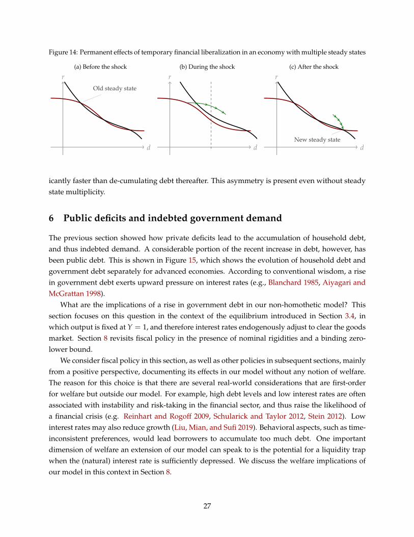
Figure 14: Permanent effects of temporary financial liberalization in an economy with multiple steady states

(a) Before the shock

d

rOld steady state

(b) During the shock

d

r(c) After the shock

d

r

New steady state

icantly faster than de-cumulating debt thereafter. This asymmetry is present even without steadystate multiplicity.

6 Public deficits and indebted government demand

The previous section showed how private deficits lead to the accumulation of household debt,and thus indebted demand. A considerable portion of the recent increase in debt, however, hasbeen public debt. This is shown in Figure 15, which shows the evolution of household debt andgovernment debt separately for advanced economies. According to conventional wisdom, a risein government debt exerts upward pressure on interest rates (e.g., Blanchard 1985, Aiyagari andMcGrattan 1998).

What are the implications of a rise in government debt in our non-homothetic model? Thissection focuses on this question in the context of the equilibrium introduced in Section 3.4, inwhich output is fixed at Y = 1, and therefore interest rates endogenously adjust to clear the goodsmarket. Section 8 revisits fiscal policy in the presence of nominal rigidities and a binding zero-lower bound.

We consider fiscal policy in this section, as well as other policies in subsequent sections, mainlyfrom a positive perspective, documenting its effects in our model without any notion of welfare.The reason for this choice is that there are several real-world considerations that are first-orderfor welfare but outside our model. For example, high debt levels and low interest rates are oftenassociated with instability and risk-taking in the financial sector, and thus raise the likelihood ofa financial crisis (e.g. Reinhart and Rogoff 2009, Schularick and Taylor 2012, Stein 2012). Lowinterest rates may also reduce growth (Liu, Mian, and Sufi 2019). Behavioral aspects, such as time-inconsistent preferences, would lead borrowers to accumulate too much debt. One importantdimension of welfare an extension of our model can speak to is the potential for a liquidity trapwhen the (natural) interest rate is sufficiently depressed. We discuss the welfare implications ofour model in this context in Section 8.

27

Figure 15: Debt by households and governments in advanced economies

0

25

50

75

100

125

1950 1960 1970 1980 1990 2000 2010 2020

Year

Household debt to GDP

Government debt to GDP

Series are cross-country averages, weighted by real GDP in 1970. The countries in the sample are Australia, Canada,Finland, France, Germany, Italy, Japan, New Zealand, Norway, Portugal, Spain, Sweden, United States and UnitedKingdom. Data come from the IMF Global Debt Database, the Jorda-Schularick-Taylor Macrohistory Database and theNew Zealand Treasury.

6.1 Incorporating the government

We introduce a standard government sector into the economy. Specifically, the government isassumed to choose a debt position Bt, government spending Gt, and proportional income taxes τi

t

on agent i such that its flow budget constraint

Gt + rtBt ≤ Bt + τst ωs + τb

t ωb

is satisfied at all times t.18 Ponzi schemes are ruled out by assuming that Bt is bounded above,uniformly in t. For simplicity, government spending is treated here as purchases of goods thatare either wasted or—which is equivalent for the purposes of this current positive exercise—enteragents’ utilities in an additively-separable form. Taxes are assumed to enter agents’ real wealth inthe natural way, rthi

t = (1− τit )ω

i + hi. Taking fiscal policy as given, the definition of a competitiveequilibrium is unchanged from before, with the exception that the bond market clearing condition

18An important question is whether government bonds in fact pay the same interest rate as other assets. To addressthis, we propose an extension in Section 9.3 that explicitly allows for a spread between government bond yields andthe return on other wealth rt.

28

Figure 16: Long-run effect of an increase in public debt B.

(a) Case with a unique steady state

d + B

r(b) Case with multiple steady states

d + B

r

is now given by dbt + ds

t + Bt = 0.

6.2 Long-run effects of fiscal policy

We begin by studying the long-run effects of fiscal policy, focusing on constant policies (G, B, τs, τb).In this case, the equilibrium conditions for steady state equilibria are given by

r = ρ1 + δ/ρ

1 + δ/ρ · η(a)(14)

a = (1− τs)ωs

r+

`(r)r

+ B (15)

Equations (14) and (15) characterize the long-run implications of fiscal policy. We are specificallyinterested in increases in B, financed by raising taxes τi on both agents or cutting expenditure G;as well as tax-financed increases in G. This yields the following result.

Proposition 6 (Long-run effects of fiscal policy on interest rates and debt.). In the long run,

a) larger government debt (B ↑) depresses the interest rate (r ↓) and crowds in household debt (d ↑).

b) tax-financed government spending (G ↑) increases the interest rate (r ↑) and crowds out householddebt (d ↓).

c) fiscal redistribution (τs ↑, τb ↓) increases the interest rate (r ↑) and crowds out household debt (d ↓).

With a homothetic saver, none of these policies have any effect on the long-run interest rate and on householddebt.

An intuition for these results can be explained with the help of Figure 16. Consider the firstpolicy in Proposition 6, and assume the greater debt level B is entirely paid for by a reductionin government expenditure G. As savers do not raise their consumption one-for-one with theincrease in debt service payments by the government, aggregate demand would fall were it not fora reduction in interest rates. Graphically, the policy corresponds to an increase in the economy’s

29

Figure 17: The lock-in effect of government debt.

(a) Small gov. debt, interest rate recovers

d + B

r(b) Large gov. debt, interest rate remains low

d + B

r

total demand for debt, d + B, which shifts out to the right (Panel (a) in Figure 16). Notably, thereduction in interest rates will crowd-in household debt.

Conversely, tax-financed government spending and fiscal redistribution reallocate resourcesfrom the saver to a “spender”, which is either the government—in the case of government spending—or the borrower—in the case of redistribution. Such resource reallocation would raise aggregatedemand were it not for an increase in interest rates.

Proposition 6 and Figure 16 prescribe a very different role for fiscal policy in influencing inter-est rates than is typically assumed. What helps in the long-run is first and foremost redistributionbetween spenders and savers, not redistribution of taxes over time in the form of public deficits,which, paradoxically, lowers long-run interest rates even further as government demand becomesindebted.

Japanification and the “lock-in” effect of government debt. Fiscal policy might not only berelevant for shifting a given steady state, but also for the existence of steady states. For example,when an economy is in a high-debt low-r steady state, then any of these policies affect not only theinterest rate associated with that steady state, but also the likelihood that another steady state—that is, one with low-debt and a higher interest rate—exists. Panel (b) of Figure 16 illustrates thisfor the case of the first policy. In this example, the increase in public debt is sufficiently large to ruleout the existence of the low-debt steady state. The intuition is even more pronounced than before.Especially if interest rates are high—as in the low-debt steady state—any significant amounts ofpublic debt constitute a drag on aggregate demand as long as their interest payments are partlycovered by borrowers.

A similar effect appears in our economy even in case of a single steady state. We illustrate thisin Figure 17. The greater government debt B is, the less the interest rate rises in response to greaterτs, lower ωs or lower `. For large B, a same-sized increase in r would require a larger adjustment ingovernment spending or taxes, reducing aggregate demand. This is why the interest rate responseto the same changes in τs, ωs or ` is smaller when B is large.

We interpret this finding as a sort of “lock-in” effect. High government debt “locks in” low

30

Figure 18: Deficit spending.

0 10 200 %

5 %

10 %

15 %

20 %

years

Gov. debt / GDP

0 10 20

3.5 %

4 %

4.5 %

5 %

5.5 %

6 %

years

Interest rate

0 10 2075 %

80 %

85 %

90 %

years

Household debt / GDP

Note. Plot shows response of non-homothetic economy to temporary government spending shock (AR(1) spendingpath with g0 = 5.5% of GDP and a half-life of 2 years). Fiscal rule: τi = r∞B where r∞ is eventual steady state interestrate.

equilibrium interest rates, a transition to higher rates becomes less likely. This effect is potentiallyan important factor in understanding the Japanese experience. Any material increase in Japaneseinterest rates would burden the government with a significant debt service cost, to finance whicha sizable fiscal adjustment would be necessary. That, however, would weigh on demand, makingthe interest rate increase unlikely in the first place.19

Fiscal policy in the analytical example. We can illustrate the effects of fiscal policy in the an-alytical example in Section 4.2. It is straightforward to obtain the steady state given a set of taxpolicies (G, B, τs, τb)

r =ρ + δ− δ

ρ ((1− τs)ωs + `)

1 + δρ B

and d =

(1 + δ

ρ B)`

ρ + δ− δρ ((1− τs)ωs + `)

.

We see that greater redistribution and greater spending (both financed through greater τs) raisesr and lowers d. Greater public debt B lowers r and crowds in d. Finally, greater B reduces thesensitivity of r to changes in τs, ωs or `.

6.3 Short run effects

Despite its novel long-run effects of government debt, the model predicts conventional short-runeffects of debt-financed fiscal stimulus programs (whether through government spending or taxcuts). As before, in terms of saving supply and debt demand curves, this is due to an upward-sloping short-run saving supply curve. We illustrate this in Figure 18, which plots the dynamicresponse of the economy to temporary deficit-financed government spending. There is a short-run rise in the natural interest rate, lasting about as long as the fiscal stimulus itself. During this

19This effect is amplified by the fact that in Japan, large scale asset purchases have shortened the duration of totalgovernment (incl. central bank) liabilities.

31

time, household debt is crowded out by higher interest rates. Afterward, however, the interestrate declines, falling below its original level and allowing debt to increase.

The opposite of the dynamics in Figure 18 would materialize in response to an austerity pro-gram, causing a short-term reduction in the natural rate but raising natural rates in the longerterm.

In practice, this suggests a dilemma for economies that are currently stuck in a steady statewith low interest rates and high public debt, but, for some reason outside our model, wish toraise rates going forward. If they expanded public debt even further, rates would rise in the shortrun, but subsequently fall again, even below their already undesirable previous levels. If theycontracted public debt, rates will fall in the short-run—possibly below the effective lower bound,causing a recession—despite the prospect of greater rates in the long run.

A possible middle ground in such a scenario may be a gradual reduction in public debt, aslong as economies are still able to do so without hitting the effective lower bound. This will allowthose governments to save some of their “fiscal policy ammunition” for the future.

7 Monetary policy and the limited ammunition effect

In the previous section, we saw that deficit-financed fiscal stimulus reduces natural interest ratesin our model in the long run. In the presence of an effective lower bound, this then implies thatthere is only a limited amount of fiscal stimulus “ammunition” that policy makers can use beforeinterest rates hit the lower bound. In this section, we show a similar “limited ammunition” prop-erty for monetary policy, by which monetary policy not only affects current output, but also thenatural interest rate going forward.

Introducing monetary policy. To do this, it is necessary to move away from an endowmenteconomy, where output Y is fixed at 1 and interest rates endogenously adjust to clear goods mar-kets. Instead, we now let output, henceforth denoted by Yt, adjust endogenously in response tomonetary policy, that is, exogenous changes to interest rates {rt}. We continue to denote potentialoutput by Y = 1. All details to the model with nominal rigidities can be found in Appendix C.3.

To allow output Yt to be endogenous, we assume it is produced using efficiency units of laborNt, Yt = Nt, which are supplied by both types of agents. We assume that dynasty i has laborproductivity ωi and supplies hours ni

t, such that total labor units are Nt = ωbnbt + ωsns

t . As inWerning (2015) and Auclert, Rognlie, and Straub (2018), Nt is allocated across agents using a sim-ple allocation rule, namely that type-i households supply hours in line with total labor demand,ni

t = Nt. We assume that prices are flexible and nominal wages are sticky.20 This implies thatreal earnings by type i are ωiYt, and thus that the income distribution is unaffected by aggregateoutput Yt. We call the allocation with Yt = Nt = 1 the natural allocation.

20The precise formulation of wage stickiness is irrelevant for our purposes as we make the simplifying assumptionbelow that monetary policy sets the real interest rate directly. See Auclert, Rognlie, and Straub (2018) for a relatedargument.

32

To ensure continued tractability of the model, we treat monetary policy as controlling the realrate directly.21 Transmission of monetary policy then works in the standard way: monetary policychanges the interest rate, which steers aggregate demand and thus output (and labor) in the econ-omy. With exogenous interest rates {rt}, the goods market now clears because {Yt} is endogenous.We define as natural interest rates the sequence of real interest rates {rn

t } that achieves the potential(or natural) allocation, that is, it implements a path of aggregate demand at potential, Yt = Y = 1.

Monetary policy shocks. To gain the most intuition about the behavior of the model, we con-sider two types of monetary policy shocks, which hit the economy at a stable steady state with(cb, cs, r, d). The first type is a T-period long interest rate reduction, before a reversal back to theoriginal interest rate

rt =

r t ≤ T

r t > T. (16)

The second type also starts with a T-period long interest rate reduction, but then reverses back tothe path of natural interest rates

rt =

r t ≤ T

rnt t > T

, (17)

ensuring that for any t > T after the intervention Yt = Y = 1 in this case.

Debt and ammunition. We begin by studying monetary policy shocks of the first kind. In ourmodel, they stimulate the economy via two separate channels. First, they relax borrowing con-straints and encourage borrowers to use additional household debt for spending (debt channel).Second, through income and substitution effects, they provide incentives for savers to spend more(saver channel). To study the role of these channels for monetary transmission, we define the fol-lowing present values

PVτ({cit}) =

∫ τ

0e−∫ t

0 rsdscitdt−

∫ τ

0e−rtcidt

PVτ({Yt}) =∫ τ

0e−∫ t

0 rsdsYtdt−∫ τ

0e−rtYdt

The first is the increase in the present value of agent i’s spending until period τ; the second is theincrease in the present value of output until period τ. The next proposition shows that the twochannels have asymmetric implications for the path of aggregate demand.

Proposition 7. The τ-period present value of the output response to the monetary policy shock (16) is given

21One can easily relax this assumption by introducing a Taylor rule and a Phillips curve, without affecting the resultsin this section. Different from a textbook New-Keynesian model, our economy is locally determinate under a real-raterule.

33

by

PVτ({Yt}) =1

ωs PVτ({cst})︸ ︷︷ ︸

saver channel

+1

ωs e−∫ τ

0 rsds (dτ − d)︸ ︷︷ ︸debt channel

. (18)

In the long run (τ = ∞), the present value of output is entirely determined by the saver channel,

PV∞({Yt}) =1

ωs PV∞({cst}). (19)

This implies that any output stimulus generated by debt accumulation necessarily weighs negatively onoutput going forward.

Proposition 7 shows that the two channels of monetary transmission have vastly differentimplications for the path of output. While the saver’s consumption response to the interest ratechange affects output permanently, the debt channel only has a temporary effect. In fact, as any ad-ditional debt taken out by borrowers eventually has to be serviced or even repaid, future demandis reduced by an active debt channel. Put differently, when monetary policy is used to stimulatethe economy, any resulting increase in demand that is debt-financed does not sustainably raisedemand and will contribute to reduced demand in the future.

One implication of the result in Proposition 7 is that if monetary policy is accommodative now,it endogenously limits its room to be accommodative in the future, as it also needs to ensure thatthe accumulated debt burden from past interventions does not cause a shortfall in demand. Theaccurate object summarizing the “room to be accommodative in the future” is the natural rate ofinterest rn

t . Our next proposition studies the effect that monetary policy has on rnt .

Proposition 8. To first order, a monetary policy shock as in (16) or (17) causes debt to rise and the naturalrate to fall, rn

t < r for any t. For a given increase in debt, the natural rate falls by more (as measured by∫ ∞s e−r(t−s)rn

t dt for any s) if there is more non-homotheticity (as measured by the elasticity εη of η); and ifinterest rates are lower (lower r) for longer (larger T).If the economy has another stable steady state with higher debt and lower interest rate, and if r is sufficientlylow and T sufficiently large, the natural rate falls permanently and does not converge back to r.

Accommodative monetary policy systematically reduces natural interest rates in our model,and thus endogenously limits the “ammunition” that is available to monetary policy in the future.This happens because in the presence of a greater debt burden, natural rates rn

t cannot possiblybe equal to r after t = T as this would tighten borrowing constraints, and lead to the borrowerseverely contracting demand. Therefore, natural rates rn

t are below r at least for some time aftert = T while the borrower deleverages (see Figure 19(a)).

This logic operates even absent non-homotheticity. However, in a homothetic model, the con-vergence process rn

t → r is sped up significantly by the fact that the saver’s consumption risessignificantly due to the increase in the saver’s permanent income, pushing the natural rate up,closer to r. In a non-homothetic model such as ours, an additional reason for a decline in rn

t

34

Figure 19: Debt limits the ammunition of monetary policy

(a) Monetary policy and natural rates

t

r

r

T

full

amm

unit

ion

monetaryintervention

possible naturalinterest rate paths

mor

ede

bt,

grea

ter

ε η

redu

ced

amm

o.

(b) Low-for-long monetary policy

d

r

for too long

too

low

convergence tolow-debt steady state

convergence tohigh-debt steady state

emerges—indebted demand—which leads to lower natural rates and a significantly reduced con-vergence rate back to r. In other words, non-homotheticity and indebted demand significantlyaggravate the “limited ammunition” property of monetary policy (see Figure 19(a)). This can besufficiently strong to permanently lower natural rates. Such behavior occurs when the economyexhibits multiple steady states, and the monetary intervention is “too low for too long”, that is, ris sufficiently low and T sufficiently long (see Figure 19(b)).

Relationship to literature. A number of economists have recently emphasized how the effec-tiveness of monetary policy interventions can be reduced by past interventions (e.g. Eichenbaum,Rebelo, and Wong 2019, Berger, Milbradt, Tourre, and Vavra 2018, McKay and Wieland 2019). Inthis paper, we do not consider consecutive interventions. Instead, we focus on how much “ammu-nition” in terms of the natural interest rate, a single intervention costs. To give an analogy with theIS curve, we focus on the effect of monetary policy on the future level of the IS curve as opposedto its slope.

Practical implications for the conduct of monetary policy. Monetary policy can have long-lasting (if not permanent) effects on natural rates through the accumulation of debt. This shouldbe taken into account when contemplating the force with which to respond to different kindsmacroeconomic shocks. Temporary shocks to borrowers’ ability to borrow for instance—e.g. dur-ing a financial crisis—can be met with aggressive monetary easing as debt is unlikely to rise inthis context. However, when reacting to shocks that do not directly affect borrowers’ demand fordebt—e.g. negative shocks to business investment as during the 2001 recession—aggressive mon-etary policy could lead to significant and persistent increases in household debt, and thereforereduce monetary policy ammunition going forward.

When used in conjunction with macroprudential policies that are designed to keep debt in

35

check, thereby dampening the debt channel, monetary policy can be used more aggressively. Thatway, the economy does not merely “pull forward” demand through debt, demand which it thenlacks in the future.

The limited power of forward guidance. In times of “limited ammunition” due to reduced nat-ural interest rates, one may wonder, whether the central bank can effectively use unconventionalpolicies such as forward guidance as a way to bring in new ammunition. To study the extent towhich this is possible, we consider monetary policy shocks as in (17) for long periods T. We havethe following result.

Proposition 9. Consider the monetary policy shock (17) as T → ∞. In the homothetic model, outputexplodes, Yt → ∞, in every period t. In the non-homothetic model output converges to a well-defined finitelimit,

Yt → YT=∞t = (ωs)−1 (r + λ + λ`(r)/ωs) (d∞ − d0) e−λ(1+`(r)/ωs)t + YT=∞

∞ (20)

where

YT=∞∞ = Y

rωs + `(r)

· η−1(ρ

r(1 + ρ/δ)− ρ/δ

), d∞ = `(r)

YT=∞∞r

.

In the homothetic economy, forward guidance is infinitely powerful, mitigating any concernsabout “limited ammunition”.22 In the non-homothetic economy, by contrast, forward guidancefaces decreasing returns in moving current output Y0 as the horizon T grows, so much so thateven a permanent interest rate cut implies a finite response of Y0. It also has well-defined long-run effects (Proposition 9). Due to indebted demand, these long-run effects can even push outputbelow potential. When the economy admits multiple stable steady states, limt→∞ Y∞

t can be belowY.

8 Debt trap and policies to escape it

The most serious implications of indebted demand occur when it tips the economy into a liquiditytrap. We next discuss ways in which an economy can slide into such a debt-driven liquidity trap,or debt trap, and evaluate policy options that may help the economy recover.

To do so, we focus on the case of our model where the interest rate associated with our model’ssteady state(s) is possibly below its effective lower bound (ELB). Let r > 0 denote that (real)effective lower bound. It needs to be positive as we take r to be the real return on wealth in ourmodel. To get a number for r, we propose to take an estimate of the real return on wealth duringthe ELB period—e.g. around 5% according to Farhi and Gourio (2018)—which then needs to bede-trended by productivity growth—e.g. 1.5%—to obtain r. In this example, r = 3.5%.

22See the extensive literature on the forward guidance puzzle, e.g. Del Negro, Giannoni, and Patterson (2015), McKay,Nakamura, and Steinsson (2016), Werning (2015), Farhi and Werning (2019), Gabaix (2019), Angeletos and Lian (2018),Bilbiie (2019), Acharya and Dogra (2019).

36

Figure 20: Falling into the liquidity trap in response to greater income inequality.

0 10 20 3080 %

85 %

90 %

95 %

100 %

years

Household debt / GDP

0 10 20 303 %

4 %

5 %

6 %

7 %

years

Interest rate

0 10 20 30−2 %

−1.5 %

−1 %

−0.5 %

0 %

years

Output gap

Without ZLB ZLB at r = 3.5%

Note. These plots simulate an increase in income inequality from ωs = 0.14 to ωs = 0.15 in the non-homotheticeconomy. The black line assumes an effective lower bound at r = 3.5% (see text).

The liquidity trap steady state. We focus on a steady state (r, d) with a natural interest rate rbelow the effective lower bound, r < r, that is,

r < ρ1 + δ/ρ

1 + δ/ρ η (ωs/r + d)(21)

In this case, the economy gives rise to a stable liquidity trap steady state, which we henceforthalso call debt trap.

Proposition 10. In the presence of an effective lower bound with (21), there exists a stable liquidity trapsteady state (“debt trap”), in which output is reduced to

Y = Yr

ωs + `(r)· η−1

(ρ

r(1 + ρ/δ)− ρ/δ

)< Y (22)

In the debt trap, household debt is high and output is permanently reduced due to indebteddemand.23 Thus, in our model, household debt is the key endogenous state variable that deter-mines whether or not an economy is able to generate sufficient demand to avoid a liquidity trap.The presence of such an endogenous state variable sets our model apart from other recent pa-pers modeling secular stagnation, e.g. Benigno and Fornaro (2019), Caballero and Farhi (2017),Eggertsson, Mehrotra, and Robbins (2019), Ravn and Sterk (2018). Moreover, the liquidity traphere is indeed a trap, meaning associated with a stable steady state, rather than a relatively briefepisode driven by household deleveraging, as in Eggertsson and Krugman (2012) and Guerrieriand Lorenzoni (2017).

23This result would be amplified in the presence of a standard Phillips curve, as in that case, a reduction in outputwould endogenously lead to weaker inflation and a tighter effective lower bound r.

37

Figure 21: Credit boom-bust cycle with subsequent liquidity trap.

0 10 20 300 %

2 %

4 %

6 %

8 %

10 %

years

Borrowing capacity (% of s.s.)

0 10 20 3090 %

92 %

94 %

96 %

98 %

100 %

years

Household debt / GDP

0 10 20 30−2 %

0 %

2 %

4 %

6 %

years

Output gap

Note. These plots simulate a permanent increase in borrowing capacity ` by 10% with fixed real interest rates at 3.5%.ωs = 14.6% to obtain a natural rate of 3.5%.

Falling into the debt trap: Inequality. Just like convergence to a steady state, our economy canfall into the debt trap. Figure 20 shows the dynamics in a simulation when in response to risingincome inequality the only stable steady state has a natural rate below the effective lower bound r.Thus, interest rates gradually fall until they hit the effective lower bound. At that point, a negativeoutput gap (i.e. a recession) begins.

Interestingly, the debt trap drags the economy into the trap even before it would have oth-erwise crossed the lower bound (blue dashed line in Figure 20). The reason for this is that bothagents anticipate a recession in the debt trap, and thus, in an attempt to smooth consumption,cut back on their spending already in advance. This, however, only accelerates the decline in thenatural rate, pushing it below the effective lower bound r sooner.

Falling into the debt trap: Credit boom & bust cycle. Another particularly relevant way aneconomy may fall into the debt trap is in the aftermath of a credit boom. To show this, consider aneconomy whose natural interest rate is exactly equal to the one at the lower bound r, and whosemonetary policy keeps the interest rate at r. This captures a monetary policy stance that happensto be “too loose” during the credit boom, which may happen for many reasons: policymakerscannot always react sufficiently quickly; they may desire to run the economy “hot”, precisely inan attempt to get away from a liquidity trap (as was commonly argued in the early 2000s); otherpolicy goals called for an accommodative stance, e.g. inflation or exchange rates.

Figure 21 shows the response of the economy with r = r to a credit boom. We model the creditboom here in its simplest possible form, namely as a permanent expansion in borrowing capacity`. This might literally capture a credit demand shock, such as a relaxation of the LTV ratio; butin a richer model with default risk this might also capture favorable credit market sentiment, asin the models of Bordalo, Gennaioli, and Shleifer (2018) and Greenwood, Hanson, and Jin (2019),and in line with the evidence in Lopez-Salido, Stein, and Zakrajsek (2017).

For a while, the economy seems to be doing well, output is increasing. Underneath the surface,

38

however, imbalances in the form of household debt accumulate. While the borrowing constraintkeeps loosening, these imbalances are masked as new debt can be used to generate demand. Assoon as borrowing capacity stops increasing, the accumulated household debt starts weighingdown on demand, rapidly pushing output below potential and pushing the economy into thedebt trap.

Crucially, the dynamics in Figure 21 play out despite our assumption that borrowing capacitylevels off but never actually falls; and despite our assumption of rational expectations. Relaxingeither of these assumptions will likely amplify the credit boom-bust cycle in Figure 21.

These considerations equally apply to increases in government debt, if those are partly fi-nanced by cutting government spending or taxing borrowers. In that case, a rapid increase ingovernment debt will fuel a boom in the economy, which—as debt begins piling up and needs tobe financed by cutting expenditure or raising taxes—then reverses into a bust. With interest ratesalready at r = r, the economy thus falls into a debt trap.

Fiscal policy in the debt trap. Once an economy finds itself in the debt trap, how does it getback out again? We can formally introduce the government exactly as in Section 6 and obtain thefollowing result.

Proposition 11. With proportional income taxes τs, τb on the saver and borrower, and a steady state levelof public debt B, output in the debt trap steady state is given by

Y = Yr

(1− τs)ωs + `(r)·[

η−1(

ρ

r(1 + ρ/δ)− ρ/δ

)− B

](23)

In particular: greater public debt lowers output in the steady state, greater redistribution through taxesraises output, and greater tax-financed government spending raises output.

This result is the mirror image of Proposition 6, except that at the effective lower bound, ad-justments in the natural rate correspond to adjustments in aggregate demand and output. One ofthe most striking predictions is that deficit-financed fiscal policy—conventionally thought to bethe best remedy against a liquidity trap—instead digs the economy even deeper into it as long asthe tax burden is not placed entirely on savers. We illustrate this behavior in Figure 22. Temporar-ily, deficit spending raises demand, bringing output closer to potential, or even above potential.Eventually, however, as the public debt burden rises, along with the associated taxes to serviceit, demand falls again, and the economy finds itself back in the debt trap. To policymakers of theconventional view, running large deficits, the liquidity trap might thus indeed feel like a “trap”,pulling the economy back into the trap after every round of deficit spending.

Redistributive tax policies and welfare. By contrast, Proposition 6 suggests that redistributivetax policies—greater τs—can raise output Y, reducing the severity of the liquidity trap. Whatwould be consequences of such a policy for the two agents? As long as the effective lower bound

39

Figure 22: Being pulled back into the liquidity trap after deficit spending.

0 2 40 %

1 %

2 %

3 %

4 %

years

Gov. spending

0 2 43 %

4 %

5 %

6 %

7 %

8 %

years

Interest rate

0 2 4

−3 %

−2 %

−1 %

0 %

years

Output gap

Note. The plot shows the response of a non-homothetic economy to a temporary government spending shock (4% ofGDP for one year). Fiscal rule: τi = r∞B where r∞ is eventual steady state interest rate. The dotted line is the previoussteady state.

is still binding, steady state consumption and wealth are given by

cs = rη−1(

ρ

r(1 + ρ/δ)− ρ/δ

)Y, as =

cs

r, cb = Y− cs. (24)

The only object that is endogenous to the tax choice is Y. Remarkably, greater redistribution there-fore leaves steady-state cs and as entirely unaffected, while boosting consumption of borrowers.The reason for this result is that the income loss of greater taxation of savers’ incomes is exactlyoffset by rising overall incomes. This can happen in the liquidity trap due to aggregate demandexternalities, as in Korinek and Simsek (2016) and Farhi and Werning (2016).

What are the implications for welfare? While (24) only holds across steady states, observethat any policy change that raises Y also relaxes the borrowing constraint and thus generatesadditional consumption for borrowers during the transition period. Moreover, one can show thatconsumption and wealth of savers are constant at the levels in (24) throughout the transition.Thus, our model implies that, in the liquidity trap, greater redistribution is Pareto-improving.

Wealth taxes. Our framework provides an interesting and novel perspective to the current de-bate (as of March 2020) surrounding wealth taxes (e.g. Saez and Zucman 2019, Guvenen, Kam-bourov, Kuruscu, Ocampo-Diaz, and Chen 2019, Sarin, Summers, and Kupferberg 2020). A (pro-gressive) wealth tax τa in our model taxes the saver’s wealth as = d + ωs

r + B each period, that is,the savers’ consolidated budget constraint (2) becomes

cst + as

t = (rt − τa) ast (25)

The returns to this policy are rebated to borrowers. As can be seen in (25), the wealth tax effectivelyreduces the after-tax return on wealth realized by savers. This changes their steady state saving

40

supply curve (10) to

r− τa = ρ · 1 + δ/ρ

1 + δ/ρ · η(as)

The relevant interest rate for savers’ saving behavior is the after-tax return on wealth r− τa. Thus,the presence of τa effectively relaxes the effective lower bound, raising output (23) during theliquidity trap according to

Y = Yr− τa

(1− τs)ωs + `(r)·[

η−1(

ρ

r− τa (1 + ρ/δ)− ρ/δ

)− B

].

Thus, a progressive wealth tax is successful in mitigating the impact of secular stagnation in ourframework.

Macroprudential policies in the debt trap. A commonly prescribed medicine for economieswith high debt burdens is macroprudential policy designed to bring down debt. As before, wethink of such financial regulation as a reduction in `. Equation (22) immediately implies thatsuch a policy raises demand and output Y in the long run, mitigating the recession. However,during the period of deleveraging, the economy goes through a significant short-run bust. Thisemphasizes that debt is best reduced by reducing saving supply rather than the demand for debt.

Borrower bailouts. An alternative way to deal with a liquidity trap caused by high levels of debtis a bailout of borrowers. We consider two such bailout strategies. A government-financed bailout ofsize ∆ > 0 is an immediate increase in public debt B by ∆, and an immediate reduction in privatedebt d by the same amount ∆. We define a debt jubilee of size ∆ > 0 as an immediate reductionin both private debt d and saver’s assets as by ∆. We assume that the public debt increase after abailout is not entirely paid for by taxing the saver (or else it would be equivalent to a debt jubilee).The following result lays out the long-run implications of bailout and debt jubilee policies:

Proposition 12 (Bailouts and debt jubilee.). Suppose the debt trap is the only steady state. A government-financed bailout lowers output in the long run. A debt jubilee raises output in the short-run, but unlesscombined with structural changes to inequality, redistribution or debt limits, there is no change to theeconomy in the long-run.

If there are multiple steady states and the economy is in the low-r high-debt steady state, a debt jubileecan raise long-run output and interest rates if its size is sufficiently large.

A debt jubilee amounts to a jump in the state variable dt. With a unique stable steady state, thiscannot have a long-run effect. In other words, borrowers would get themselves into debt again.However, a debt jubilee has positive short run effects, as it lifts the economy temporarily out ofthe debt trap. To prevent it from falling into it again, it needs to be paired with other policies, e.g.redistributive or macroprudential policies (see above). Such a combination can jointly addressshort and long-run issues. A government-financed bailout increases long-run public debt andtherefore lowers long-run output, as in Proposition 11.

41

Things are somewhat more subtle with steady state multiplicity. Here, if ∆ is sufficiently large,a debt jubilee, i.e. a jump in dt, can put the economy on a permanently different trajectory, towardsa different steady state. This also works for a government-financed bailout, with the caveat thatwhen public debt is too large, another steady state, one with higher r and lower d, might cease toexist (see our discussion in Section 6.2).

Summary: Policy implications of a debt trap. All in all, we find that the traditional macroe-conomic policy toolbox reaches its limits in a debt trap. Conventional monetary policy is, perdefinitionem, constrained. Unconventional monetary policy, such as forward guidance, is less ef-fective than previously thought, were the debt trap to end at some point. We have not includedan analysis of quantitative easing in the present paper, but its effects are likely captured by a re-duction in the return on wealth r that can be earned during a debt trap. It would mitigate theimmediate output loss, but not address the structural problem of high debt levels and low interestrates. Finally, conventional deficit spending only works if it is financed in a progressive way. Inthe model, this requires taxing savers. In reality, this could require raising top marginal incometax rates, better enforcement of estate taxes, or introduction of wealth taxes.

Some policy tools outside the traditional toolbox, however, gain in importance. Redistributivepolicies and structural changes to reduce income inequality are effective in sustainably generatingmore demand, and thus can prevent debt traps and effectively lead economies out of them. Simi-larly effective are tax-financed government spending and productive government investment (seethe next section below). Macroprudential policies succeed in preventing economies from fallinginto a debt trap, but can worsen the recession in the short run when already in a debt trap.

9 Extensions

Our baseline model was intentionally kept simple. Next we discuss several extensions to ourbaseline model. We begin with two generalizations of the supply side of our economy, introducinggrowth and investment.

9.1 Growth

To introduce growth into our model, we assume that each real asset (tree) now bears Yt = egt

fruits, instead of Y = 1. For any quantity x (e.g. consumption, assets, asset prices) denote by xits de-trended version, that is, xt ≡ e−gtxt. As usual, the de-trended budget constraint of type iagents is then

cit + ˙ai

t ≤ (rt − g)ait.

42

Crucially, as we continue to assume that preferences are over wealth relative to income, v(ait/Yt),

as discussed in Section 3.5, we can express preferences (1) as function of de-trended variables,

∫ ∞

0e−(ρ+δ)t

{gt + log

(ci

t/µi)+

δ

ρv(ai

t/µi)

}dt

where clearly the term gt is irrelevant for consumption choices. Finally, the de-trended price of atree is

pt ≡∫ ∞

teg(s−t)−

∫ st rududs.

Following exactly the same steps as before, we can derive two conditions that characterize thesteady state(s) with growth. As it turns out, both equations are simply shifted versions of theconditions without growth. The saving supply and debt demand curves now read

r− g = ρ · 1 + δ/ρ

1 + δ/ρ · η(ωs/(r− g) + d)and d =

`(r− g)r− g

(26)

where we now write ` as a function of r − g since common microfoundations (e.g. those in Ap-pendix C.2) would precisely predict such a relationship. Equation (26) shows that growth is or-thogonal to the steady states in our model. It merely shifts both curves vertically in parallel.Similarly, one can show that growth does not change the dynamics of the economy either, afterde-trending.

9.2 Investment

Having studied the effects of growth, we now turn to a different extension of the supply side ofour economy, namely allowing for capital and investment. To do so, we allow output Y to beproduced from three factors, capital K and both types of agents’ labor supply Li, and we write thenet-of-depreciation production function as24

Y = F(K, Lb, Ls).

We assume that without loss that Y has constant returns to scale; otherwise we include a fixedfactor owned by savers and/or borrowers. Thus, total income Y can be split up into income goingto savers and income going to borrowers. As we assume that labor supplies Li are fixed, theincome shares only depend on the level of capital K, which itself is pinned down by the interestrate,

FK = r.24We assume the typical: F is strictly concave, satisfying Inada conditions.

43

Further, in our economy, only savers hold capital. The agents’ income shares are then functions ofthe interest rate and given by

ωs(r) =FKK

F+

FLs Ls

Fand ωb(r) =

FLb Lb

F= 1−ωs(r).

With these income shares, we can now characterize our economy’s steady states as

r = ρ · 1 + δ/ρ

1 + δ/ρ · η(ωs(r)/r + d)and d =

`(r)r

. (27)

Crucially, ωs(r) is now possibly a function of r. As we demonstrate in the following proposition,the shape of ωs(r) depends on the (Allen) elasticity of substitution σ ≡ FLb FK/(FKLb F) betweencapital and borrowers’ labor supply.

Proposition 13. Let σ be the elasticity of substitution between capital and borrowers’ labor supply in theeconomy with investment. Denote by ωs(r) the savers’ income share.

a) If σ = 1: ωs(r) is independent of the interest rate r. All steady state(s) are identical to the economywithout investment.

b) If σ < 1: ωs(r) falls with lower r. This flattens the saving supply curve.

c) If σ > 1: ωs(r) rises with lower r. This steepens in the saving supply curve.

Proposition 13 precisely characterizes the role of investment for the long-run economy. Whenan increase in capital leaves the income distribution unchanged, investment will have no effect onthe long-run (case (a)). So to what extent capital matters depends on whether it crowds the shareof income going to borrowers in or out. If capital is complementary to borrowers’ labor supply, itreduces the extent of indebted demand (even if it can never fully undo it) as lower interest rates gohand in hand with greater capital and a more equitable income distribution (case (b)). If capital issubstitutable with borrowers’ labor supply—one may think of capital-skill complementarity andautomation as in Krusell, Ohanian, Rios-Rull, and Violante (2000) and Autor, Levy, and Murnane(2003),—the opposite is the case. Lower interest rates endogenously lead to a more unequal in-come distribution, effectively steepening the saving supply curve and amplifying the problem ofindebted demand (case (c)).25 We illustrate the three cases in Figure 23.

This discussion focused on the long run. Investment contributes to demand in the short runas interest rates fall, irrespective of the structure of the production function F. For example, if Fis Cobb-Douglas, and the economy sees a shift in income inequality, investment picks up initially,temporarily slowing the decline in r. As the investment boom recedes, however, the fall in raccelerates again, eventually falling to the exact same steady state level as would have occurredwithout investment (as in Section 5).

25See Straub (2019) for a related point.

44

Figure 23: Capital and indebted demand

d

r

σ = 1σ > 1

σ < 1

Observe that the recent US experience does not align well with this description of investment(see Figure 3). It did not seem that investment rose as interest rates fell. This is subject of arecent literature (Gutierrez and Philippon 2017, Liu, Mian, and Sufi 2019, Farhi and Gourio 2018,Eggertsson, Robbins, and Wold 2018).

Which kind of debt causes indebted demand? Productive vs. unproductive debt. Investmentmay be funded with (corporate) debt, raising the question, which kind of debt actually causes in-debted demand? In Section 4, we argued that, starting in some steady state, a one-time exogenousincrease in debt by some dD, holding r fixed, causes a response of aggregate spending of

dC = −ρ + δ

2

(1−

√1− 4

(1− r

ρ + δ

)εη

)dD (28)

(see Proposition 13). The debt in this experiment is unproductive, that is, it is being used for con-sumption.

We now repeat this exercise with productive debt, that is, debt that is being used to raise thecapital stock of the economy, dK = dD. Holding r and household debt d fixed, what are theimplications for aggregate spending?

Proposition 14 (Indebted demand when debt is productive). Starting from a steady state and holdingr and d, fixed, an exogenous increase in debt dD that raises the capital stock by the same amount affectsaggregate spending by

dC = −ρ + δ

2

(1−

√1− 4

(1− r

ρ + δ

)εηχ

)dD. (29)

where χ ≡(1− σ−1)ωb − r rd

Y < 1.

A first observation about Proposition 14 is that productive debt, (29), always causes strictlyless indebted demand than unproductive debt, (28). To see this, note that χ =

(1− σ−1)ωb −

r rdY < 1. Thus, even if capital is perfectly substitutable with borrowers’ labor supply, σ = ∞,

productive debt does not cause as much indebted demand. The reason for this is that even if

45

σ = ∞, capital raises aggregate output. A second observation is that the negative effect of dDon aggregate spending dC falls for lower values of σ, as one would expect given (13). In thecase σ = 1, the effect is positive at first, dC > 0. Recall that (29) is the contemporary effect onspending—but once we allow household debt to increase with Y, the positive effect fades.

The distinction between productive and unproductive debt is not always obvious. Consider,for example, investments in infrastructure (e.g. airports, buildings, trains) in remote locations,as some argue can be found in China today. Debt that is financing such investments ought bethought of as unproductive.

A special case where debt is used productively but χ is still very high is residential investmentinto borrowers’ owner-occupied housing. For example, imagine borrowers remodel or extendtheir houses. Clearly this is productive, as a greater housing stock produces more housing ser-vices. However, these additional housing services are consumed by borrowers themselves and donot increase borrowers’ marginal product of labor. Thus, in this case, σ = ∞ and χ = ωb − r rd

Y ,the largest possible value for productive debt.

In sum, our results suggest that productive debt always causes weaker indebted demand thanunproductive debt. The degree to which it is weaker depends on the elasticity of substitution σ

between the capital that is accumulated using debt and the borrowers’ labor supply. This suggeststhat debt-financed productive investments made by firms or governments need not necessarilycontribute to indebted demand.

Does student debt contribute to indebted demand? Since the end of the Great Recession, the UShas witnessed a significant increase in student debt, begging the question whether student debt isa likely contributor to indebted demand. At the face of it, it seems that the answer is no. After all,student debt finances investment in human capital, and thus can be analyzed like investment inphysical capital.

There is, however, an important difference. The rise in student debt partly reflects the risingcost of college tuition. To the extent this is the case, student debt is indeed a source of indebteddemand, as borrowers have to service larger piles of student debt without having accumulatedgreater human capital.

9.3 Risk premia and convenience yields

A concern one might have with our fiscal policy results is that they were derived in a model inwhich government bonds pay the same return as any other asset, while this is clearly not the casein the data. What, for instance, if there is a spread between the overall return on wealth r and thereturn on government bonds rB? How does this impact our predictions for fiscal policy?

We allow for such a spread by assuming that savers, who are the equilibrium holders of gov-ernment bonds, derive an additional utility from holding government bonds, as in Krishnamurthyand Vissing-Jorgensen (2012). In particular, since savers derive utility from both consumption and

46

wealth, we assume the per-period utility function of a representative saver is

log ((cst + ξBt) /µs) + δ/ρv ((as

t + ξBt/r) /µs) .

The saver’s Euler equations now differ for bonds and other assets. In the steady state, weobtain

0 = rB + ξ − ρ− δ +δ

ρrη (a + ξB/r) (30)

for government bonds and

0 = r− ρ− δ +δ

ρrη (a + ξB/r) (31)

for other assets. Subtracting (31) from (30) yields a steady-state government bond return of

rB = r− ξ. (32)

Due to the spread ξ in (32), rB is always strictly lower than r. Thus, it might hit zero even as r isstill positive. We distinguish two cases, depending on whether rB is positive or zero.

Steady states without ZLB (positive rB). The steady states in this economy turn out to be exactlythe same as before, characterized by the intersections of the exact same two curves,

r = ρ1 + ρ/δ

1 + ρ/δ · η(a)and a = (1− τs)

ωs

r+

`(r)r

+ B. (33)

That is, an increase in government debt B shifts out the demand curve for borrowing, pushingdown the long-run return on wealth r, and through (32), also the return on government debt.

The reason for this finding is simple. There is a positive spread in (32) since savers derivetangible benefits from investing in government bonds. These benefits, however, make savers ef-fectively richer, offsetting the reduction in saver wealth due to lower interest income (r − ξ)Bfrom government bonds. Thus, when the benefits are included, the value of government bondsfor savers is indeed B and not rBB/r.

While the steady state curves (33) are unaffected, the spread in (32) obviously affects the gov-ernment budget constraint. In particular, financing a steady-state public debt position B now onlycosts (r− ξ)B instead of rB.26 This becomes especially relevant in a liquidity trap.

Steady states with binding ZLB (zero rB). We can use the model with government bond spreadsto revisit the liquidity trap (“debt trap”). In Section 8 we assumed there to be an effective lowerbound r > 0 for the return on wealth r. In this economy, we can now explicitly impose a zero lowerbound for the government bond yield rB. Given (32), this is fully consistent with our previousapproach when r = ξ.

26Paradoxically, this might even raise the effect of B on steady state return on wealth r as τs adjusts by less in (33).

47

Thus, as before, a debt trap steady state exists if the natural allocation would require a negativegovernment bond yield rB < 0, or equivalently, r < ξ. The result in Proposition 10 carries over tothis economy, meaning output in the debt trap is given by

Y = Yr

(1− τs)ωs + `(ξ)·[

η−1(

ρ

ξ(1 + ρ/δ)− ρ/δ

)− B

](34)

and therefore still decreasing in B.There is, however, a new policy option on the table now, which was absent in Section 8. As gov-

ernments pay zero interest rates on their bonds, rB = 0, they can effectively run a Ponzi scheme:permanently raise government spending G by an amount equal to the shortfall in demand torestore the natural allocation, Y = Y, financed by an ever-growing pile of government debt.

While this is a perfectly well-defined equilibrium in theory, it is risky in practice, not the leastbecause a high public debt to GDP ratio might expose the government to rollover crises (unmod-eled here) even if interest rates rB are expected to remain low for long. There is also no exit strategy.As (34) highlights, the longer a government runs the Ponzi scheme, the more significant the out-put loss when exiting will be. In addition, as we demonstrate in Section 6.2, a recovery to greaterequilibrium interest rates is more unlikely when government debt is large.

9.4 Intergenerational mobility

We have so far ignored mobility across saver and borrower dynasties. Yet, since current mobilitylevels in the US are low while income inequality is rising (Lee and Solon 2009, Chetty, Hendren,Kline, Saez, and Turner 2014), several policies have been proposed to promote intergenerationalmobility. To study the effects of such policies on household debt and interest rates, we next extendour framework to include mobility.

To do so without jeopardizing the tractability of our model, we assume that with some prob-ability q > 0, savers’ offsprings turn into borrowers; and with probability q µ

1−µ , borrowers’ off-springs turn into savers. A saver-turned-borrower immediately consumes his wealth down to thelevel of an average borrower ab/(1− µ); and vice versa, a borrower-turned-saver immediately re-ceives a transfer from all savers to achieve their average asset position as/µ.27 Agents’ preferencesare unchanged.

This structure changes the saving supply curve to

r = ρ1 + δ/ρ

1 + δ/ρη(a)+ qγδ

δ/ρη(a)1 + δ/ρη(a)︸ ︷︷ ︸

contribution of mobility

(35)

where γ is a measure of steady-state income inequality, equal to 1 minus the ratio of per capita

27This may be interpreted as borrowers marrying into saver families.

48

incomes

γ = 1−(ωb − `

)/ (1− µ)

(ωs + `) /µ.

We see from (35) that the intergenerational mobility term increases in a. This makes the savingsupply curve less downward-sloping, thus mitigating indebted demand. The effect of greatermobility (raising q) is particularly relevant when income inequality γ is high, i.e. close to 1, sincein that case, it redistributes wealth within each generation in a similar fashion as redistributivetaxation.

9.5 Open economy model

Many countries with large debt burdens are open economies. This begs the question whetherour model can be generalized to an open economy setting, and if so, whether this generates newinsights. This is what we briefly discuss next.

We assume that our two types of agents live in a small open economy (the “home” country),which trades a single good with the rest of the world. It has imperfect access to world financialmarkets: as in Gabaix and Maggiori (2015), a continuum of foreign-based financial intermediariesinvests in the home country, earning a return spread equal to the domestic interest rate r minusthe world interest rate r∗. Thus, home’s net foreign asset position is given by

nfat =1Γ[r∗ − rt] . (36)

What do steady states look like in this economy? To understand this, it helps to view therest of the world as another “borrower” in the economy. When the home interest rate rt is lowerthan the world interest rate r∗, the rest of the world borrows an amount equal to nfat from thehome economy. Thus, nfat expands total steady-state saving demand to dt + Bt + nfat. Given(36), opening up the economy’s financial account amounts to a counterclockwise twist around thepoint on the saving demand curve where r = r∗.

International credit boom-bust cycle. A similar open economy extension can be developed withnominal rigidities, in the spirit of Gali and Monacelli (2005), but with imperfect international cap-ital markets as in (36). In that extension, a permanent expansion in ` would also induce a boom-bust cycle—much like the one in the closed economy in Section 8. Assuming that monetary policyfollows a standard Taylor rule, the boom-bust cycle will be more pronounced in an open economy,due to amplification from capital flows. In particular, as the economy booms, imports and interestrates rt rise, pulling in additional capital, which is ultimately lent to borrowers. Then, as borrow-ers start to cut back on their spending, and rt falls, capital flows reverse and leave the countryagain. This international credit cycle bears similarities with the evidence in Mian, Sufi, and Verner(2017).

49

9.6 Longer duration debt

A recent literature highlighted that responses of economies to interest rate changes differ accord-ing to the type of debt contract agents hold (e.g. adjustable-rate vs. fixed-rate contracts) as wellas the debt’s maturity (e.g. Campbell 2013, Calza, Monacelli, and Stracca 2013, Di Maggio et al.2017). In this extension, we investigate the role of debt duration for indebted demand. We assumethat all debt is fixed rate, and is being rolled over at Poisson rate λ. Since asset duration is irrel-evant for the steady state(s), we focus on two transitional dynamics experiments: one of fallingreal interest rates and increasing debt levels (e.g. due to rising income inequality as in Figure 11)and one of rising real interest rates and falling debt levels (e.g. due to redistributive taxation). Forboth experiments, we ask whether fixed-rate debt (FR) would speed up the transition relative toadjustable-rate debt (AR), or slow it down.

To study the first experiment, when a shock suddenly lowers real interest rates relative towhat they were expected to be, this does not affect the present value of AR debt, but pushes upthe present value of FR debt. Formally, this means the state variable d jumps up on impact of theshock. Such a jump corresponds to a fast transition in practice. Since the present value increaseswithout any actual increase in debt originations, the additional demand typically associated withstrong credit growth is absent in this case.

To study the second experiment, consider a shock that pushes real interest rates up. Thepresent value of AR debt is again unchanged, but the present value of FR debt falls, again speed-ing up the transition. Thus, in some sense AR debt makes it harder to leave a steady state withhigh levels of debt since any increase in interest rates leads to an immediate sharp fall in demandwithout favorable revaluation effect.

These discussions highlight that AR debt contracts slow down transitions into states with lowr and high debt, and FR debt contracts speed up transitions away from such states. Fixed-ratecontracts with automatic refinancing achieve both of these arguably favorable outcomes.28 Policiesthat raise the share of refinancing among US fixed-rate mortgage owners are therefore beneficialfrom this perspective.

10 How indebted is demand in practice?

Measuring the slope of the saving supply curve. The key ingredient to our theory is the downward-sloping saving supply curve. This begs the question of whether one can get a sense of the mag-nitude of the slope of the saving supply curve. To investigate this, we employ a simple sufficientstatistics approach.

Let C(r, a) be the steady state consumption of rich households in an economy (e.g. the top 5%or top 1%). The definition of the saving supply curve r(a) as function of rich households’ wealth

28Lengthening the maturity of debt when debt is high, as in Campbell, Clara, and Cocco (2018), would furtherspeed up transitions back to lower debt states as they would lengthen the duration of debt. Automatic refinancingis reminiscent of the idea to convert FR into AR contracts (Guren, Krishnamurthy, and McQuade 2017), albeit such aconversion would slow down transitions back to states with lower debt levels.

50

requires thatC(r(a), a) = r(a)a.

Total differentiation of this equation with respect to a allows us to isolate the local slope of thesaving supply curve

drd log a

=MPCcap. gains − r

1− εrca

where εr ≡ ∂ log c∂r is the rich’s semi-elasticity of consumption with respect to a permanent shift in

interest rates, and MPCcap. gains is the MPC out of wealth of the rich. To get a sense of magnitudes,we assume εr = 0, which would be implied by log preferences. The MPCcap. gains should be in-terpreted as an MPC out of an increase in capital gains as most wealth gains for the very richesthouseholds come in the form of capital gains. We use the estimate from Chodorow-Reich, Nenov,and Simsek (2019) for this MPC, MPCcap. gains = 0.028, which is in the same ballpark as the esti-mates of Baker, Nagel, and Wurgler (2007) and Di Maggio, Kermani, and Majlesi (2019). Finally,recent estimates of the real return on wealth are on the order of 5-7% (Farhi and Gourio 2018). Wetake r = 6% for this exercise.

Together this simple calculation implies an estimate for the local slope of the saving supplycurve

drd log a

≈ −0.032.

In words, this implies that if the richest households’ wealth rises by 10%, the interest rate has tocome down by 32 basis points. While this is certainly not a precise calculation, it gives a roughsense of the magnitudes that are at play in our model.

Implications for indebted demand in the US. A way to get a sense the extent of indebted de-mand in the US is to evaluate the hypothetical demand shortfall from high debt levels, had realinterest rates not fallen since 1980. In the spirit of Proposition 3, we thus ask: if debt levels were ashigh as they are today, with interest rates still at 1980 levels, how much smaller would aggregatespending dC + dG be?

To conduct this exercise, we need to know the hypothetical debt service costs that would haveprevailed absent a fall in interest rates. We compute this for every year since 1980 in Figure 24,finding significant increases in hypothetical debt service costs, both for household and govern-ment debt. Together, they have amounted to 15% of household disposable income in recent years.Thus, with the same MPCcap. gains estimate and r, the demand shortfall is in the ballpark of

dC ≈ −15%︸ ︷︷ ︸borrower debt service

+MPCcap. gains

r· 15%︸ ︷︷ ︸

partial offset by savers

= −8%

This is a significant number, which would rationalize why the natural interest rate indeed had todecline significantly in order for debt burdens not to depress demand.

51

Figure 24: Hypothetical debt service costs had interest rates not declined.

10

15

20

Pe

rce

nt

1980 1990 2000 2010 2020

Household DSR

Household DSR (counterfactual)

Household

0

5

10

15

20

Pe

rce

nt

1980 1990 2000 2010 2020

Government DSR

Government DSR (counterfactual)

Government

See Appendix A for details.

11 Conclusion

In this paper, we proposed a new theory connecting several recent secular trends: the increase inincome inequality, financial liberalization, the decline in natural interest rates, and the rise in debtby households and governments.

The central element in our theory are non-homothetic preferences, which lead to richer house-holds having greater saving rates out of a permanent income transfer. This gives rise to the idea ofindebted demand: greater debt levels mean a greater transfer of income in the form of debt servicepayments from borrowers to savers, and thus depress demand.

We identified three main implications of indebted demand. First, secular economic shifts thatraise debt levels (e.g. income inequality or financial liberalization) also lower natural interest rates,which then itself has an amplified effect on debt. Second, monetary and fiscal policy, to the extentthat they involve household or government debt creation, can persistently reduce future naturalinterest rates. This means that there is only a limited number of such policy interventions that canbe used before economies approach the effective lower bound. Finally, when the lower bound isbinding, the economy is in a debt-driven liquidity trap with depressed output. In this “debt trap”,debt-financed stimulus deepens the recession in the future, whereas redistributive policies andpolicies addressing the structural sources of inequality mitigate it.

Our results suggest that economies face a sort of “budget constraint for aggregate demand”.They can stimulate aggregate demand through debt creation, but that reduces future demand (andthus natural interest rates). This logic suggests a new trade-off for debt-based stimulus policies.We view an exploration of this trade-off in an optimal policy setting as a promising avenue forfuture research.

52

References

Acharya, S. and K. Dogra (2019). Understanding hank: Insights from a prank. Working Paper.

Achdou, Y., J. Han, J.-M. Lasry, P.-L. Lions, and B. Moll (2017). Heterogeneous agent models incontinuous time. Manuscript.

Aiyagari, S. R. and E. McGrattan (1998). The optimum quantity of debt. Journal of MonetaryEconomics 42(3), 447–469.

Angeletos, G.-M. and C. Lian (2018). Forward guidance without common knowledge. AmericanEconomic Review 108(9), 2477–2512.

Auclert, A. and M. Rognlie (2018). Inequality and aggregate demand. Technical report, NationalBureau of Economic Research.

Auclert, A., M. Rognlie, and L. Straub (2018). The intertemporal keynesian cross.

Autor, D., F. Levy, and R. J. Murnane (2003). The skill content of recent technological change: Anempirical exploration. Quarterly Journal of Economics.

Baker, M., S. Nagel, and J. Wurgler (2007). The Effect of Dividends on Consumption. BrookingsPapers on Economic Activity 38(1), 231–292.

Ball, M. (1990). Under one roof: retail banking and the international mortgage finance revolution. Har-vester Wheatsheaf.

Bartscher, A. K., M. Kuhn, M. Schularick, and U. I. Steins (2018). Modigliani meets minsky: Amer-ican household debt, 1949-2016. Working Paper.

Benhabib, J., A. Bisin, and M. Luo (2019). Wealth distribution and social mobility in the us: Aquantitative approach. American Economic Review 109, 1623–47.

Benigno, G. and L. Fornaro (2019). Stagnation traps. The Review of Economic Studies, forthcoming.

Beraja, M., A. Fuster, E. Hurst, and J. Vavra (2018). Regional Heterogeneity and the RefinancingChannel of Monetary Policy. The Quarterly Journal of Economics 134(1), 109–183.

Berger, D., K. Milbradt, F. Tourre, and J. Vavra (2018). Mortgage prepayment and path-dependenteffects of monetary policy. Working Paper.

Bernanke, B. S. (2005). The global saving glut and the U.S. current account deficit. Speech 77,Board of Governors of the Federal Reserve System (U.S.).

Bernanke, B. S. and M. Gertler (2001). Should central banks respond to movements in asset prices?American Economic Review 91(2), 253–257.

Bhutta, N. and B. J. Keys (2016). Interest rates and equity extraction during the housing boom.American Economic Review 106(7), 1742–74.

Bilbiie, F. O. (2019). Monetary policy and heterogeneity: An analytical framework. Working Paper.

Blanchard, O. (1985). Debt, deficits, and finite horizons. Journal of Political Economy 93(2), 223–247.

Boar, C. (2018). Dynastic precautionary savings. Manuscript.

53

Bokhari, S., W. Torous, and W. Wheaton (2013). Why did household mortgage leverage rise fromthe mid-1980s until the great recession. In American Economic Association 2013 Annual Meeting.San Diego, California. Citeseer.

Bordalo, P., N. Gennaioli, and A. Shleifer (2018). Diagnostic expectations and credit cycles. TheJournal of Finance 73(1), 199–227.

Borio, C. and P. Disyatat (2014). Low interest rates and secular stagnation: is debt a missing link?VoxEU.

Borio, C. and W. White (2004). Whither monetary and financial stability? the implications ofevolving policy regimes. BIS Working Papers.

Bourguignon, F. (1981). Pareto superiority of unegalitarian equilibria in stiglitz’model of wealthdistribution with convex saving function. Econometrica: Journal of the Econometric Society, 1469–1475.

Caballero, R. and E. Farhi (2017). The safety trap. The Review of Economic Studies 85(1), 223–274.

Caballero, R. J. and A. Simsek (2019). Prudential monetary policy. Technical report, NationalBureau of Economic Research.

Cairo, I. and J. Sim (2018). Income inequality, financial crises, and monetary policy.

Calza, A., T. Monacelli, and L. Stracca (2013). Housing finance and monetary policy. Journal of theEuropean Economic Association 11(S1), 101–122.

Campbell, J. Y. (2013). Mortgage market design. Review of Finance 17(1), 1–33.

Campbell, J. Y., N. Clara, and J. F. Cocco (2018). Structuring mortgages for macroeconomic stability.Manuscript.

Carroll, C. (2000). Why do the rich save so much?

Chetty, R., N. Hendren, P. Kline, E. Saez, and N. Turner (2014). Is the united states still a land ofopportunity? recent trends in intergenerational mobility. American Economic Review: Papers andProceedings 104(5), 141–147.

Chodorow-Reich, G., P. T. Nenov, and A. Simsek (2019). Stock market wealth and the real econ-omy: A local labor market approach.

Cloyne, J., C. Ferreira, and P. Surico (2019). Monetary Policy when Households have Debt: NewEvidence on the Transmission Mechanism. The Review of Economic Studies.

Coeurdacier, N., S. Guibaud, and K. Jin (2015). Credit constraints and growth in a global economy.American Economic Review 105(9), 2838–81.

Cole, H. L., G. J. Mailath, and A. Postlewaite (1992). Social norms, savings behavior, and growth.Journal of Political economy 100(6), 1092–1125.

Dalio, R. (2018). Principles For Navigating Big Debt Crises. Bridgewater.

De Nardi, M. (2004). Wealth inequality and intergenerational links. The Review of Economic Stud-ies 71(3), 743–768.

54

De Nardi, M., E. French, J. B. Jones, and A. Gooptu (2011). Medicaid and the elderly. Technicalreport, National Bureau of Economic Research.

Del Negro, M., M. Giannoni, and C. Patterson (2015). The forward guidance puzzle. WorkingPaper.

Di Maggio, M., A. Kermani, B. J. Keys, T. Piskorski, R. Ramcharan, A. Seru, and V. Yao (2017). In-terest rate pass-through: Mortgage rates, household consumption, and voluntary deleveraging.American Economic Review 107(11), 3550–88.

Di Maggio, M., A. Kermani, and K. Majlesi (2019). Stock market returns and consumption. Journalof Finance.

Di Maggio, M., A. Kermani, and C. Palmer (2019). How quantitative easing works: Evidence onthe refinancing channel. The Review of Economic Studies, forthcoming.

Dynan, K. E., J. Skinner, and S. P. Zeldes (2004). Do the rich save more? Journal of PoliticalEconomy 112(2), 397–444.

Eggertsson, G. B. and P. Krugman (2012). Debt, deleveraging, and the liquidity trap: A Fisher-Minsky-Koo approach. Quarterly Journal of Economics 127(3), 1469–1513.

Eggertsson, G. B., N. R. Mehrotra, and J. A. Robbins (2019). A model of secular stagnation: Theoryand quantitative evaluation. American Economic Journal: Macroeconomics 11(1), 1–48.

Eggertsson, G. B., J. A. Robbins, and E. G. Wold (2018). Kaldor and piketty’s facts: the rise ofmonopoly power in the united states. Working Paper.

Eichenbaum, M., S. Rebelo, and A. Wong (2019). State dependent effects of monetary policy: therefinancing channel. Working Paper.

Erceg, C. J., D. W. Henderson, and A. T. Levin (2000). Optimal monetary policy with staggeredwage and price contracts. Journal of monetary Economics 46(2), 281–313.

Fagereng, A., M. B. Holm, B. Moll, and G. Natvik (2019). Saving behavior across the wealthdistribution: The importance of capital gains.

Farhi, E. and F. Gourio (2018). Accounting for macro-finance trends: Market power, intangibles,and risk premia. Brookings Papers on Economic Activity Fall, 147–250.

Farhi, E. and I. Werning (2016). A theory of macroprudential policies in the presence of nominalrigidities. Econometrica 84(5), 1645–1704.

Farhi, E. and I. Werning (2019). Monetary policy, bounded rationality, and incomplete markets.American Economic Review, forthcoming.

Favilukis, J., S. C. Ludvigson, and S. Van Nieuwerburgh (2017). The macroeconomic effects ofhousing wealth, housing finance, and limited risk sharing in general equilibrium. Journal ofPolitical Economy 125(1), 140–223.

Gabaix, X. (2019). A behavioral new keynesian model. Working Paper.

Gabaix, X. and M. Maggiori (2015, 03). International liquidity and exchange rate dynamics. Quar-terly Journal of Economics 130(3), 1369–1420.

55

Gali, J. and T. Monacelli (2005). Monetary policy and exchange rate volatility in a small openeconomy. Review of Economic Studies 72, 707–734.

Greenwald, D. (2018). The mortgage credit channel of macroeconomic transmission.

Greenwood, R., S. G. Hanson, and L. J. Jin (2019). Reflexivity in credit markets.

Guerrieri, V. and G. Lorenzoni (2017). Credit crises, precautionary savings, and the liquidity trap.The Quarterly Journal of Economics 132(3), 1427–1467.

Guren, A. M., A. Krishnamurthy, and T. J. McQuade (2017). Mortgage design in an equilibriummodel of the housing market. Working Paper.

Gutierrez, G. and T. Philippon (2017). Investment-less growth: An empirical investigation. Tech-nical report, Brookings Papers on Economic Activity.

Guvenen, F., G. Kambourov, B. Kuruscu, S. Ocampo-Diaz, and D. Chen (2019). Use it or lose it:Efficiency gains from wealth taxation. Technical report, National Bureau of Economic Research.

Iachan, F. S., P. T. Nenov, and A. Simsek (2015). The choice channel of financial innovation. Tech-nical report, National Bureau of Economic Research.

Illing, G., Y. Ono, and M. Schlegl (2018). Credit booms, debt overhang and secular stagnation.European Economic Review 78(104).

Jorda, O., M. Schularick, and A. M. Taylor (2015). Betting the house. Journal of International Eco-nomics 96, S2–S18.

Jorda, O., M. Schularick, and A. M. Taylor (2016). The great mortgaging: housing finance, crisesand business cycles. Economic Policy 31(85), 107–152.

Justiniano, A., G. E. Primiceri, and A. Tambalotti (2017). The mortgage rate conundrum. WorkingPaper.

Katz, L. F. and K. M. Murphy (1992). Changes in relative wages, 1963–1987: supply and demandfactors. The Quarterly Journal of Economics 107(1), 35–78.

King, M. and D. Low (2014). Measuring the”world”real interest rate. Technical report, NationalBureau of Economic Research.

Koo, R. (2008). The Holy Grail of Macroeconomics - Lessons from Japan’s Great Recession. Wiley.

Koopmans, T. C. (1960). Stationary ordinal utility and impatience. Econometrica: Journal of theEconometric Society, 287–309.

Korinek, A. and A. Simsek (2016). Liquidity trap and excessive leverage. American EconomicReview 106(3), 699–738.

Krishnamurthy, A. and A. Vissing-Jorgensen (2012). The aggregate demand for treasury debt.Journal of Political Economy 120(2).

Krusell, P., L. E. Ohanian, J.-V. Rios-Rull, and G. L. Violante (2000). Capital-skill complementarityand inequality: A macroeconomic analysis. Econometrica 68(5), 1029–1053.

56

Kumhof, M., R. Ranciere, and P. Winant (2015). Inequality, leverage, and crises. American EconomicReview 105(3), 1217–45.

Lee, C.-I. and G. Solon (2009, November). Trends in Intergenerational Income Mobility. The Reviewof Economics and Statistics 91(4), 766–772.

Liu, E., A. Mian, and A. Sufi (2019). Low interest rates, market power, and productivity growth.Working Paper.

Lo, S. and K. S. Rogoff (2015). Secular stagnation, debt overhang and other rationales for sluggishgrowth, six years on. BIS Working Papers.

Lopez-Salido, D., J. C. Stein, and E. Zakrajsek (2017). Credit-market sentiment and the businesscycle. The Quarterly Journal of Economics 132(3), 1373–1426.

Lucas, R. E. J. and N. L. Stokey (1983). Optimal fiscal and monetary policy in an economy withoutcapital. Journal of Monetary Economics 12(1), 55–93.

McKay, A., E. Nakamura, and J. Steinsson (2016). The power of forward guidance revisited. Amer-ican Economic Review 106(10), 3133–3158.

McKay, A. and J. Wieland (2019). Lumpy durable consumption demand and the limited ammuni-tion of monetary policy. Working Paper.

Mian, A., L. Straub, and A. Sufi (2019). The saving glut of the rich and the rise in debt.

Mian, A. and A. Sufi (2015). House of debt: How they (and you) caused the Great Recession, and how wecan prevent it from happening again. University of Chicago Press.

Mian, A., A. Sufi, and E. Verner (2017). Household debt and business cycles worldwide. TheQuarterly Journal of Economics 132(4), 1755–1817.

Piketty, T. (2014). Capital in the Twenty-First Century. Belknap Press: An Imprint of Harvard Uni-versity Press.

Piketty, T. and E. Saez (2003). Income inequality in the united states, 1913-1998. Quarterly Journalof Economics.

Piketty, T., E. Saez, and G. Zucman (2017). Distributional national accounts: methods and esti-mates for the united states. The Quarterly Journal of Economics 133(2), 553–609.

Rachel, L. and L. H. Summers (2019). On falling neutral real rates, fiscal policy and the risk ofsecular stagnation. In Brookings Papers on Economic Activity BPEA Conference Drafts, March 7-8.

Rannenberg, A. (2019). Inequality, the risk of secular stagnation and the increase in householddebt. Working Paper.

Ravn, M. and V. Sterk (2018). Macroeconomic fluctuations with hank and sam: An analyticalapproach. Working Paper.

Reinhart, C. M. and K. S. Rogoff (2009). This Time is Different: Eigth Centuries of Financial Folly.Princeton University Press.

Reinhart, C. M. and K. S. Rogoff (2010). Growth in a time of debt. American economic review 100(2),573–78.

57

Saez, E. and S. Stantcheva (2018). A simpler theory of optimal capital taxation. Journal of PublicEconomics 162, 120–142.

Saez, E. and G. Zucman (2016). Wealth inequality in the united states since 1913: Evidence fromcapitalized income tax data. The Quarterly Journal of Economics 131(2), 519–578.

Saez, E. and G. Zucman (2019). Progressive wealth taxation. Brookings Papers on Economic Activity.

Sarin, N., L. Summers, and J. Kupferberg (2020). Tax reform for progressivity: A pragmatic ap-proach. Tackling the Tax Code: Efficient and Equitable Ways to Raise Revenue.

Schularick, M. and A. M. Taylor (2012). Credit booms gone bust: Monetary policy, leverage cycles,and financial crises, 1870-2008. American Economic Review 102(2), 1029–61.

Stein, J. C. (2012). Monetary policy as financial-stability regulation. Quarterly Journal of Eco-nomics 127(1), 57–95. forthcoming in the Quarterly Journal of Economics Draft Date: RevisedMay 2011.

Stein, J. C. (2013). Overheating in credit markets: Origins, measurement, and policy responses.Speech at Federal Reserve Bank of St Louis.

Stiglitz, J. E. (1969). Distribution of income and wealth among individuals. Econometrica: Journalof the Econometric Society, 382–397.

Straub, L. (2019). Consumption, savings, and the distribution of permanent income.

Strotz, R. H. (1956). Myopia and inconsistency in dynamic utility maximization. The Review ofEconomic Studies 23(3), 165–180.

Summers, L. H. (2014). Us economic prospects: Secular stagnation, hysteresis, and the zero lowerbound. Business Economics 49(2), 65–73.

Svensson, L. E. (2018). Monetary policy and macroprudential policy: Different and separate?Canadian Journal of Economics 51(3), 802–827.

Turner, A. (2015). Between Debt and the Devil: Money, Credit, and Fixing Global Finance. PrincetonUniversity Press.

Uzawa, H. (1968). Market allocation and optimum growth. Australian Economic Papers 7(10), 17–27.

Von Schlicht, E. (1975). A neoclassical theory of wealth distribution. Jahrbucher fur Nationalokonomieund Statistik 189(1-2), 78–96.

Werning, I. (2015). Incomplete markets and aggregate demand. Working Paper.

58

Appendix

A Data and figures

Figure 24. Quarterly, seasonally adjusted data on disposable personal income (DPI) are obtainedfrom the US Bureau of Economic Analysis. Levels and debt service ratios (DSR) for householdmortgage debt and consumer credit debt are obtained from the Board of Governors of the FederalReserve System. In these data, the overall DSR is by definition the sum of household mortgage andconsumer credit DSRs, and debt service ratios are calculated as debt service payments as a percentof DPI. Following the methodology used by the Federal Reserve, we take the level of consumercredit debt for households and nonprofit organizations (LA153166000 in Financial Accounts ofthe United States) and the level of mortgage debt as total mortgages to households and nonprofitorganizations (FL153165005 in Financial Accounts of the United States).

For each of household mortgages (HM) and consumer credit (CC), we assume that there is aconstant amortization rate δd and a fixed interest rate rd,t, which determine the debt service ratio,equal to:

DSRd,t =Dd,t × (rd,t + δd)

DPIt,

where d is a type of debt, DPIt is disposable personal income and Dd,t is the level of debtat time t. Note again that DSRHM,t and DSRCC,t sum to the total household debt service ratioDSRHH,t.

We build a counterfactual series under the premise that rd,t remained constant over time, fixedat 1980 Q1 levels. We use this to recalculate the counterfactual DSRs for the two types of debt, asfollows, with dots denoting counterfactual:

¨DSRd,t =Dd,t × (rd,1980Q1 + δd)

It

Finally, we sum these to obtain ¨DSRHH,t = ¨DSRHM,t + ¨DSRCC,t. The left panel of Figure 24plots DSRHH,t and ¨DSRHH,t.

For the government’s debt service ratio, we conduct a similar analysis using total governmentdebt DG,t and government interest payments IPG,t. Government in this case refers solely to thefederal government. We define the government debt service ratio DSRG,t to be:

DSRG,t =IPG,t

DPIt.

We decompose the government debt service ratio in the same manner as we do for households:

DSRG,t =DG,t × (rG,t + δG)

DPIt

We build the government’s counterfactual DSR series under the assumption that rG,t remainedconstant at 1980Q1 levels. Precisely,

59

¨DSRG,t =DG,t × (rG,1980Q1 + δG)

DPIt

The right panel of Figure 24 plots DSRG,t and ¨DSRG,t.

B Proofs

Proof of Proposition 1. This proof is an immediate consequence of (10).

Proof of Proposition 2. Given that debt d > 0, savers cannot be up against their borrowingconstraint. Thus, the Euler equation has to hold with equality, implying (11). Moreover, the Eulerequation cannot hold with equality for borrowers, as their per capita wealth is much smaller thanthat of savers. Thus, their borrowing constraint is binding, implying (12)

Proof of Proposition 3. As borrowers are borrowing constrained, their consumption respondsone for one, dcb = −dx. To analyze the consumption response by savers define their consumption-wealth ratio χt ≡ cs

t /ast . Expressing budget constraint and Euler equation in terms of (as

t , χt), wefind

ast

ast= r− χt and

χt

χt= χt − ρ− δ +

δ

ρχtη(as

t).

To get the on-impact consumption response of savers, we need to solve the ODEs for a smallchange in wealth at date 0 away from the steady state, in which χ∗ = r and r = ρ+ δ− δ/ρrη(as∗).Let a, χ be the deviations (in levels, not logs) from the steady state. Defining εη ≡ η′(as∗)as∗/η(as∗),we have

˙at = −as∗χt and ˙χt = (ρ + δ) χt + (ρ + δ− r) rεηat

as∗ . (37)

We guess and verify that χ = −ka/as∗ for k > 0. Using the equations in (37) we find a quadraticfor k,

k2 − (ρ + δ) k + (ρ + δ− r)rεη = 0.

The only solution that leads to a positive consumption response to transfers is

k =ρ + δ

2

(1−

√1− 4

(1− r

ρ + δ

)εη

).

Since cst = as∗χt + rat = (r− k)at, and a0 = dx/r, we have

dcs0 = dx− k/rdx

which together with dcb0 implies (13).

Local uniqueness and existence result. Here we prove that locally around a stable steady state,i.e. for d0 in a neighborhood of steady-state debt d∗, there is a unique equilibrium. To do this,we first collect the equations describing equilibrium when the borrower is up against a bindingborrowing constraint. We focus on the special case with `(pt) = ` = const; the general case of a

60

stable steady state when `(pt)pt increases in pt follows analogously. The pricing equation for realassets is

rt pt = 1 + pt. (38)

The debt level evolves asdt = λ`pt − λdt (39)

which we can plug into the savers’ collective budget constraint, we get the interest rate

rt =1dt{cs

t + λ`pt − λdt −ωst} . (40)

Finally, savers’ Euler equation is given by

cst

cst= rt − ρ− δ + δ

cst

ρ (ωs pt + dt)η(ωs pt + dt). (41)

Equations (38)–(41) describe a system of 3 ODEs in variables (pt, dt, cst), after using (40) to substi-

tute out the interest rate rt. Denote by (p∗, d∗, cs∗) the respective steady state values of the threevariables. We define two auxiliary variables

w ≡ ωs

`and ∆ ≡ ρ + δ− r∗.

In the homothetic model, ∆ = 0. Using them, we find for the steady state variables

p∗ =1r∗

, d∗ =`

r∗,

c∗

d∗= r∗(1 + w),

p∗

d∗=

1`

.

Denote by p, d, cs the log-linearized versions of p, d, cs. Denote by r the linearized version of r.Linearizing (38)–(41) we find

r = −r∗d + cr∗(1 + w) + λ p− λd

˙p = r + r∗ p (42)

˙d = λ p− λd

˙c = r + ∆[

c−(1− εη

) wp + dw + 1

]We guess and verify that the solution takes the form

r = −Rd, p = Pd, c = Cd.

We also verify that ˙d/d < 0, which is necessary for an equilibrium in the neighborhood of thesteady state. After some algebra, we arrive at a condition for P,

F(P) = 0

61

where

F(P) = [∆ + λ (2− P) + r∗(1 + w)] (λ(1− P) + r∗) P + ∆Pλ

− λ(∆ + λ(1− P))− r∗λ + r∗∆[(1− εη) (1 + Pw)− 1

].

As one can see easily, F(0) < 0, F(1) > 0, F′′(1) < 0, F′′′(0) > 0 (the coefficient on P3 is positive).Together, they imply that F admits a unique root P below 1. This root is therefore unique inimplying stability, ˙d/d = λ(P− 1) < 0. It also implies that

R = Pλ(1− P) + r∗P > 0, (43)

so that the (natural) interest rate is lower if the economy has a higher debt level than steady statedebt. Moreover, observe that F strictly declines in εη . Thus,

∂P∂εη

> 0. (44)

Proof of Proposition 4. The proof is an immediate consequence of Proposition 2.

Proof of Proposition 5. The proof is an immediate consequence of Proposition 2.

Proof of Proposition 6. This follows directly from (14) and (15).

Proof of Proposition 7. Savers’ intertemporal budget constraint is given by∫ τ

0e−∫ t

0 rsdscitdt = ωs

∫ τ

0e−∫ t

0 rsdsYtdt + d0 − e−∫ τ

0 rsdsdτ (45)

which implies (18) by subtracting from (45) its steady state analogue. (19) is a direct consequenceof (18) and the fact that the steady state is stable, and so dτ → d as τ → ∞.29

Proof of Proposition 8. To start, we derive the system of equations characterizing the evolutionof the economy in response to an arbitrary path of interest rates rt. From the savers’ budgetconstraint and Euler equation we have

ast = rtas

t − cst

cst

cst= rt − ρ− δ + δ

cst

ρastη (as

t) .

As one can easily see in a phase diagram (Figure 25), both equations are forward looking. Thus,under a monetary policy shock as in (16), cs

t and ast jump up on impact, converging back towards

their steady state values, cst = cs and as

t = as, which they reach at t = T. Noting that ast = ωs pt + dt,

we find that debt evolves asdt = −λ(1 + w−1)dt + w−1as

t (46)

29Stability of a steady state for a fixed interest rate r follows from (46) below. For fixed r, ast is immediately at its

steady state value (see discussion below and Figure 25).

62

Figure 25: Phase diagram for (cst , as

t) under an exogenous interest rate.

ast

cst

csT = 0 locus

asT = 0 locus

cs0 = 0 locus

as0 = 0 locus

implying that dt > d for all t > 0 (w ≡ ωs/`). Thus, under a monetary policy shock as in (16), debtstrictly rises. An (first-order) increase in debt, as explained in (43), leads to a reduction in naturalinterest rates.

The increase in debt is greater for all t under monetary policy shock (17). The reason for thisis that under (16), natural rates are still below steady state r after t = T. Thus, if rt = rn

t is setafter t = T, rt is below what it would be under (16). But if rt is lower, both as

t and cst are greater

everywhere (Figure 25), which by (46) must translate into a greater level of debt. Similarly, if weincrease T or reduce r, this further raises cs

t and ast in Figure 25, thus also increasing the path of

debt dt at all times.Why do natural rates fall more with greater non-homotheticity? To prove this, we focus on a

convenient measure of the path of natural rates, namely the present value, Rns ≡ r

∫ ∞s e−r(t−s)rn

t dt.We ask: how does Rn

s ≡ Rns − r vary with the level of debt d? And how does that mapping depend

on εη? By (42), we find thatRn

t = −rPdt.

Thus, natural interest rates always fall when dt > 0, and more so the larger P is, e.g. when εη isgreater (see (44)).

Finally, consider a situation with multiple steady states. Call r the interest rate of the alternativehigh-debt, low-interest-rate steady state, and cs, as, d the associated values of cs, as and d. Basedon Figure 25, setting r = r forever (T = ∞) means cs

t = cs and ast = as for any t > 0. Both variables

jump immediately to their new values. Debt evolves as in (46), and converges to d. Because thenew steady state is stable, the economy does not converge back to its original values. Also, bycontinuity, there exists a threshold T, such that any T > T will bring the economy sufficientlyclose to d that it will converge by itself (without any further stimulus) to the alternative steadystate.

Proof of Proposition 9. As explained above, for fixed r, cst and as

t jump immediately to their newvalues cs

∞, as∞. Solving (46), we find

dt = d0e−λ(1+w−1)t +as

∞λ(1 + w−1)

(1− e−λ(1+w−1)t

)for the path of debt. This gives us the path of asset prices from pt =

as∞−dtωs and output from

Y = r∞ pt − p.

63

After some algebra, this yields (20).

Proof of Proposition 10. The expression for Y follows directly from inverting saving supplycurve at r,

r = ρ1 + δ/ρ

1 + δ/ρη(

ωs+`(r)r Y

)to solve for Y. The debt trap is stable since the economy, for a fixed interest rate r, is described byconstant cs, as, and debt evolves as in (46), converging always back to the debt trap debt level.

Proof of Proposition 11. (23) again follows directly from inverting the saving supply curve withfiscal policy at r,

r = ρ1 + δ/ρ

1 + δ/ρη((1−τs)ωs+`(r)

r Y + B) .

Proof of Proposition 12. A partial or full debt jubilee has no effect in the long run as the economywill always converge back to the unique debt trap steady state. A (government-financed) bailoutlowers output in the long run as it increases government debt B (Proposition 11).

If there are multiple steady states, there is a threshold for debt d∗ (equal to that of the second-largest-debt steady state), such that if the jubilee moves the economy to a debt level d0 ≤ d∗,long-run output and interest rates are greater than before.

Proof of Proposition 13. The result follows directly from (27) and the behavior of ωs(r). Observethat

∂ωs

∂K= −∂ωb

∂K=(

1− σ−1)

ωb FK

Y(47)

implying that ωs increases with K (and falls with r) precisely iff σ > 1, and is constant if σ = 1.The slope of the saving supply curve is given by

∂r∂d

= − δη′r

ρ + δη − δη′ ωs(r)r + δη′ωs′(r)

where η, η′ are evaluated at ωs(r)/r + d. Evidently, the larger (more positive) ωs′(r) is, the flatteris the saving supply curve. Vice versa for negative ωs′(r).

Proof of Proposition 14. To derive (29), observe that

∂ (as/Y)∂D

=∂

∂D

(ωs

r+

rdY

)=(

1− σ−1)

ωb − rdY

FK

Y=(

1− σ−1)

ωb − rrdY≡ χ

where we used (47). Following steps as in the proof of Proposition 3, we then find that the savers’consumption response to the increase in their assets dD is given by

dcs0 = (r− k)dD

64

where now

k =ρ + δ

2

(1−

√1− 4

(1− r

ρ + δ

)εηχ

).

Thus, dC = −kdD.

C Model extensions

C.1 More general preferences

C.1.1 EIS different from one

Our model naturally generalizes to utility functions over consumption with an elasticity of in-tertemporal substitution (EIS) σ−1 different from one. Assume the preferences of a type-i agentare given by ∫ ∞

0e−(ρ+δ)t

{1

1− σ

(ci

t/µi)1−σ

+δ

ρσv(ai

t/µi)

}dt.

Define η(a) ≡ (a/µs)σv′(a/µs) so that the homothetic benchmark with v′(a) ∝ a−σ continues tocorrespond to η(a) = 1. The Euler equation of savers is then given by

σcs

tcs

t= rt − ρ− δ + δ

(cs

tρas

t

)σ

η(ast)

which, at a steady state, reduces to

r = ρ + δ− δ

(rρ

)σ

η(as).

While not necessarily solvable in closed form for r, this equation still has a unique solution for r forany value of as, by the intermediate value theorem. Moreover, by the implicit function theorem,the slope of the implied saving supply curve is still negative.

C.1.2 Recursive preferences over consumption

Our preferences (1) involve a warm-glow utility over bequests. Does the negative slope of thesaving supply curve hinge on bequests (or wealth more broadly) entering the utility function? Wenow argue that the answer is no. To do so, we give both agents a recursive utility function solelydefined over consumption, as in Uzawa (1968) and Lucas and Stokey (1983). We thus assumepreferences are given by

Ui =∫ ∞

0u(ci

t/µi)e−∆t dt

where ∆t = ρ(ci

t/µi), u is strictly increasing, continuously differentiable and concave, and ρ iscontinuously differentiable. If ρ = const, this corresponds to standard homothetic preferences,but in general, these preferences allow the discount factor to move with consumption.

After some math, we find that savers’ steady state Euler equation is

r = ρ(ras/µs).

This defines an implicit equation in r for any ai. If ρ decreases, such that greater consumption

65

levels are associated with less impatience, the saving supply curve is downward-sloping, just asin the model of Section 3.

C.1.3 Preferences over relative wealth

As we mentioned in Section 3.5, an alternative way to set up the warm-glow bequest utility is todefine it not relative to output Y, but relative to total wealth. In this formulation, preferences aregiven by ∫ ∞

0e−(ρ+δ)t

{log(

cit/µi

)+

δ

ρv(

ait/µi

At

)}dt

where we let At ≡ ast + ab

t . Observe that A = Y/r = 1/r in a steady state (Y is normalized to 1).Defining η as before, we then obtain the savers’ Euler equation and saving supply curve

cst

cst= rt − ρ− δ + δ

cst

ρastη

(ai

tAt

)⇒ r = ρ

1 + δ/ρ

1 + δ/ρη (ras). (48)

The only change in (48) relative to (10) is that there is now an additional “r” on the right hand side.Conceptually, this plays no role, however. When η(a) is increasing, the right hand side falls in r,implying that there is a unique interest rate r for any as. Moreover, as the right hand side also fallsin as, that interest rate must decline as as increases. Thus, we still have a negatively sloped savingsupply curve.

C.2 Borrowing constraints nested

We provide three alternative microfoundations for a borrowing constraint that fits our generaldescription in (8).

C.2.1 Housing as collateral asset

In Section 3, we derived a simple borrowing constraint based on the idea that agents can pledgean income stream `Y (e.g. coming from land they own). We now show that one would obtain asimilar borrowing constraint when borrowers purchase houses instead, and use them as collateral.To do so, assume there is a fixed mass µb of housing units, freely traded at price ph

t , over whichborrowers have additive preferences α log ht each period, α > 0. We assume that the collateralconstraint is d + λd ≤ θph

t ht, where θ is the loan-to-value (LTV) ratio. In steady state, one canshow that this implies a market clearing house price

ph(r) =αωb

(1− θ/λ)ρ + (1 + α)θr/λ

This fits into our earlier framework by assuming that `(r) = rph(r).In this version of the model, agents in the borrower dynasty bequeath both the house and their

debt position to their offsprings. In a more realistic model with a life-cycle, older agents wouldsell their house, pay down their debts and consume the proceeds before death. Younger agentswould purchase houses, partly debt-financed. A larger house price (due to lower interest rates),would stimulate consumption of existing homeowners and sellers of houses, raising aggregateconsumption of the borrower dynasty, even if younger agents now pay more for the same-sizedhouse.

66

C.2.2 Bewley-Aiyagari model

For this extension, we model borrowers as in Achdou, Han, Lasry, Lions, and Moll (2017), that is,we deviate from homogeneous preferences across types of agents. We focus on a steady state witha constant interest rate r. Each borrower i maximizes utility

E0

∫ ∞

0e−ρt log ci

tdt

subject to budget and borrowing constraint

dit = rdi

t + cit − ybei

t and dit ≤ dyb

where d > 0 and eit > 0 is a random Markov process for productivity in continuous time; yb ≡

ωbY/µb is borrowers’ average income. This specification implies that borrowers can borrow up toa fixed fraction (or multiple) of their average income. Following the logic in Achdou et al. (2017),we see that total debt taken out by borrowers, d(r, yb) ≡

∫di

tdi in a steady state with rate r iscontinuous and approaches −∞ as r ↑ ρ and approaches dyb as r ↓ 0. Moreover, observe thatd(r, yb) scales in yb due to homothetic preferences, see Straub (2019). Therefore, we can write totaldebt as

d(r, yb) = d(r, 1)yb = rd(r, 1)ωb/µb︸ ︷︷ ︸≡`(r)

·Yr

in line with our general borrowing constraint (8). Thus, this model generates a steady-state debtdemand curve that is “mostly” downward-sloping, in the sense that d(r, yb) is−∞ for r ↑ ρ, risingto dyb for r ↓ 0. There could be non-monotonicity in between, although that is unlikely given theresults in Achdou et al. (2017).

C.2.3 Simplified buffer stock model

We have found that a simplified and tractable version of the full Bewley-Aiyagari model is auseful way to understand its implications. Specifically, we assume that there is a small Poissonprobability υ > 0 that a borrower receives a one-time negative income shock of size ϕY > 0 (afterwhich there are no more other shocks). We model the negative shock to be sufficiently large that itshows up in a borrower’s asset position: when assets are ab

t before the shock, they fall to abt − ϕY

after the shock. As we make the shock probability very small, υ → 0, this setup converges to amodel where the borrowing constraint is given by

dit + λdi

t ≤ pt`− ϕY

where the borrowing constraint is tightened by the potential income loss ϕY relative to (7). Theright hand side can be rewritten in the form `({rs}s≥t).

C.3 Nominal rigidities

Households. We describe the model with nominal rigidities here in more detail. First, agentspreferences are given by∫ ∞

0e−(ρ+δ)t

{log(

cit/µi

)+

δ

ρv(ai

t/µi)− φ

1 + η−1

(ni

t

)1+η−1}dt (49)

67

where η is the Frisch elasticity of labor supply, and φ is a disutility shifter. Observe that in thelimit η → 0, this model converges to an endowment economy, with labor endowments ni

t = 1 peragent. The budget constraint is still given (2) with a total asset position equal to

ait = hi

t − dit.

Real asset wealth, which is equal to human wealth here, is given by

rhit = wtω

init + hi

t (50)

where wt is the real wage per efficiency unit and ωi/µi denotes the efficiency units per hourworked of dynasty i. Total efficiency units supplied by dynasty i are then ωini

t. Combining (2)and (50), we can also write the budget constraint in the more traditional form,

cit + rtdi

t ≤ dit + wtω

init (51)

To be consistent with this description, the price of pledgable wealth is then assumed to be equalto

pt ≡∫ ∞

te−∫ s

t ruduwsnisds (52)

with the interpretation that a total amount ` < ωi of efficiency units can be pledged by eachdynasty. This implies the same borrowing constrained as before, (7).

Production. Production in this economy follows a simple linear aggregate production function

Yt = Nt

where Nt equals total efficiency units supplied by the dynasties, Nt = ωbnbt + ωsns

t . We assumeproduction is perfectly competitive and prices are flexible, so that the real wage is equal to 1 at alltimes, wt = 1.

Nominal rigidities and monetary policy rule. Instead, we assume that nominal wages are per-fectly rigid, Wt = 1. While this might seem extreme, our results will be amplified if a Phillipscurve is assumed instead.30 With a wage rigidity in place, workers may be off their labor supplycurves, so it is important to determine which worker works how much. Here, we keep with theexisting literature, e.g. Werning (2015) and Auclert, Rognlie, and Straub (2018), and assume thatboth dynasties’ hours move identically, nb

t = nst = Nt = Yt. The central bank in this model sets a

path for the real interest rate {rt} directly (as in Auclert, Rognlie, and Straub 2018).Observe that with these modifications, the above modeling equations can be simplified. For

instance, the budget constraint (51) becomes

cit + rtdi

t ≤ dit + ωiYt

and the price of pledgable wealth (52) becomes

pt ≡∫ ∞

te−∫ s

t ruduYsds

30This can be for instance done by integrating the heterogeneous-agent version of the Erceg, Henderson, and Levin(2000) wage rigidity model developed in Auclert, Rognlie, and Straub (2018).

68

Natural allocation. The natural allocation is defined as the allocation that would materialize ifwages were perfectly flexible. In that case, rt is no longer determined by monetary policy. Withlabor supply as in (49), wealth effects on labor supply imply that the natural allocation need notnecessarily feature ni

t = 1 and thus not necessarily Yt = Y = 1. To establish continuity with ouranalysis before and focus on the case where the natural allocation indeed exhibits Yt = Y = 1, wefocus on the case where η → 0. This assumption essentially makes labor supply arbitrarily curvedaround 1. While not having any effects on our analysis of monetary policy, it does imply that thenatural allocation is one in which ni

t = 1 for both dynasties, implying that dynasty i’s income isequal to ωi just as in the endowment economy introduced in Section 3.

69