indefinite metric sp ces in estima -...
TRANSCRIPT

INDEFINITE METRIC SPACES IN ESTIMATION�
CONTROL AND ADAPTIVE FILTERING
a dissertation
submitted to the department of electrical engineering
and the committee on graduate studies
of stanford university
in partial fulfillment of the requirements
for the degree of
doctor of philosophy
By
Babak Hassibi
August ����

c� Copyright ����
by
Babak Hassibi
ii

I certify that I have read this thesis and that in my opin�
ion it is fully adequate� in scope and in quality� as a
dissertation for the degree of Doctor of Philosophy�
Thomas Kailath�Principal Adviser
I certify that I have read this thesis and that in my opin�
ion it is fully adequate� in scope and in quality� as a
dissertation for the degree of Doctor of Philosophy�
Stephen P� Boyd
I certify that I have read this thesis and that in my opin�
ion it is fully adequate� in scope and in quality� as a
dissertation for the degree of Doctor of Philosophy�
Ali H� Sayed
I certify that I have read this thesis and that in my opin�
ion it is fully adequate� in scope and in quality� as a
dissertation for the degree of Doctor of Philosophy�
Nick W� McKeown
Approved for the University Committee on Graduate
Studies
Dean of Graduate Studies
iii

Abdol
iv

Abstract
The goal of this thesis is two�fold �rst� to present a uni�ed mathematical framework
�based upon optimization in inde�nite metric spaces for a wide range of problems in
estimation and control� and second� to motivate and introduce the problem of robust
estimation and control� and to study its implications to the area of adaptive signal
processing�
Robust estimation �and control is concerned with the design of estimators �and
controllers that have acceptable performance in the face of model uncertainties and
lack of statistical information� and can be considered an outgrowth and extension of
�the now classical LQG theory� developed in the ��� �s and ��� �s� which assumed
perfect models and complete statistical knowledge� It has particular signi�cance in
adaptive signal processing where one needs to cope with time�variations of system
parameters and to compensate for lack of a priori knowledge of the statistics of the
input data and disturbances� One method of addressing the above problem is the
so�called H� approach� which was introduced by G� Zames in ��� and that has
been recently solved by various authors�
Despite the �fundamental di�erences� between the philosophies of the H� and
LQG approaches to control and estimation� there are striking �formal similarities�
between the controllers and estimators obtained from these two methodologies� In an
attempt to explain these similarities� we shall describe a new approach to H� esti�
mation �and control� di�erent from the existing �e�g�� interpolation�theoretic�based�
game�theoretic�based� etc� approaches� that is based upon setting up estimation
�and control problems� not in the usual Hilbert space of random variables� but in an
inde�nite �so�called Krein space�
v

The Krein space formulation provides a uni�ed approach for problems in LQG�
H�� risk�sensitive� and game�theoretic� estimation and control� and� most impor�
tantly� allows one to use the insight obtained from over three decades of work in
traditional LQG theory to obtain new results in these other areas� Proceeding in
this spirit� we demonstrate how to generalize the �possibly numerically superior
square�root algorithms and the fast Chandrasekhar algorithms to the H� setting�
and embark on some new investigations on the asymptotic behaviour of H� �lters
and controllers� and on the existence and properties of solutions of Riccati equations
with �possibly inde�nite coe�cient matrices�
We also study adaptive �ltering using the H� approach to robust estimation
and show that the celebrated LMS �least�mean squares adaptive algorithm is H��
optimal� This result solves the long standing issue of �nding a rigorous basis for
LMS �which was long thought to be an approximate least�squares solution� It also
suggests some further rami�cations� such as the design of robust adaptive �lters with
more desirable tracking properties� as well as some directions for further research�
such as the mixed H��H� problem�
vi

Acknowledgements
The work presented in this thesis would not have been possible without the support�
in�uence and encouragement of numerous individuals � mentors� colleagues� friends
and family � that I have had the great fortune of interacting with during my �ve
year stay at Stanford� And so� this is now an opportunity to acknowledge� in indeed
a very small way� my debt to all these persons�
First� and foremost� I would like to express my deep gratitude to my advisor and
mentor� Professor Thomas Kailath� for constant and generous� support� encourage�
ment and guidance� not only in technical matters� where the depth of his knowledge is
truly profound� but also in nontechnical matters� and in the inevitable ups and downs
that occur during any such PhD endeavor� His provocative questions� thoughtful dis�
cussions� and careful comments and criticisms� have greatly in�uenced my thought�
and are re�ected throughout the presentation of this thesis� I am also grateful for the
opportunities he has provided for me to interact with other distinguished researchers�
both in this country and abroad�
I would also like to thank Professor Stephen Boyd for serving as my associate
advisor� for being on my orals and reading committees� and� especially� for some
of the most stimulating courses that I have attended at Stanford� His clarity and
style in presenting technical material is something that I have always admired and
wished to emulate� I am also grateful to Professor Ali Sayed for serving on my orals
and reading committees� During my second� and unquestionably most technically
productive� year at Stanford I had the great fortune of closely interacting with Ali�
and so� many of the results presented in this thesis are joint work with him� I am also
grateful to Professor Nick McKeown for serving on my orals and reading committees�
vii

despite what must certainly have been a very busy schedule� and for venturing to
read a dissertation in an area quite removed from his research interests�
Special thanks are due to Professors Pramod Khargonekar and David Limebeer for
very useful comments and discussions on the initial stages of this work� to Professors
Lennart Ljung and Karl Astrom for critical discussions on the results of Chapter ��
and to Professors Patrick Dewilde� Jan Willems� Bill Helton and James Rovnyak for
their valuable comments and feedback on many of the results of this thesis�
Special thanks are also due to Professor Arogyaswami Paulraj for many useful
discussions and interesting seminars� and so also to Drs� Guanghan Xu� Lang Tong�
Young Man Cho� Buno Pati� Allejan Van der Veen and Vadim Olshevsky�
I am greatly indebted to my former and current o�ce�mates in Durand � �B�
Hamid Aghajan� Tibor Boros� Babak Khalaj� Poogyeon Park and Greg Raleigh for
creating a friendly and stimulating work atmosphere� and for many �often late night
discussions� and also to my other dear friends in ISL� especially� Jalil Kamali and
Bijit Halder� I also gratefully acknowledge the e�cient assistance� help and patience
of Christine Lincke and Karen Ariente�
I am also very grateful to Drs� David Stork and Peter Hart� and Greg Wolf� of
the Ricoh California Research Center� where I spent a Summer internship in ����� for
stimulating discussions on the topic of neural networks� and for much encouragement
during my �rst few years at Stanford� I also had the great fortune of spending
a very fruitful stay at the Indian Institute of Science at Bangalore� India� and so
would like to gratefully acknowledge the warm hospitality of Professor V�U� Reddy�
and the graduate students �now dispersed across the globe� of the Electrical and
Communications Department at that institute�
My many friends in the Stanford community have also had an important� albeit
indirect� in�uence on the development of this thesis� I am especially grateful to
Masoud Zargari� Mehrdad Heshami� Babak Ebrahimian� Rasool Khadem� Hossein
Sedarat� Behnam Tabrizi� Hadi Taheri and Behfar Razavi�
My deepest gratitude� love and a�ection belong� of course� to my parents Jamshid
and Farzaneh� to whom� as I begin to realize more and more each year� I owe all that
I am and all that I have ever accomplished� And so to my brother Arash� with whom
viii

I have had the great fortune of being reunited at Stanford during the past two years�
to my brother Arjang� and to the memory of my late grandfather� Kazem Hassibi�
who has been the greatest inspiration in education for us all� My deep gratitude
also goes to my uncles� Drs� Hossein Naraghipour� Houshang Hassibi and Khosrow
Hassibi� who have helped to make possible my education in the US� And for my dear
wife� Faranak� whose love� care and patience have inspired and supported me over
the years� both when we were on opposite sides of the globe� and now that we here
are together� my gratitude is beyond words�
Finally� I should mention that� since childhood� I was always impressed by the
dedication on the �rst page of my father�s ���� PhD thesis� and so am honored to
follow in his footsteps� and to dedicate this thesis to �those who support education
at all levels for all��
ix
Contents
Abstract v
Acknowledgements vii
� Introduction �
��� Some Historical Remarks � � � � � � � � � � � � � � � � � � � � � � � � � �
��� A Basic Estimation Problem � � � � � � � � � � � � � � � � � � � � � � � �
����� Special Cases � � � � � � � � � � � � � � � � � � � � � � � � � � � �
��� The H� Approach � � � � � � � � � � � � � � � � � � � � � � � � � � � � � ��
����� The General Solution � � � � � � � � � � � � � � � � � � � � � � � ��
����� Special Cases � � � � � � � � � � � � � � � � � � � � � � � � � � � ��
����� The Question of Robustness � � � � � � � � � � � � � � � � � � � ��
��� The H� Approach � � � � � � � � � � � � � � � � � � � � � � � � � � � � ��
����� The General Solution � � � � � � � � � � � � � � � � � � � � � � � ��
����� Special Cases � � � � � � � � � � � � � � � � � � � � � � � � � � � ��
��� Control Problems � � � � � � � � � � � � � � � � � � � � � � � � � � � � � ��
����� Full Information Control � � � � � � � � � � � � � � � � � � � � � ��
����� Measurement Feedback Control � � � � � � � � � � � � � � � � � ��
����� Special Cases � � � � � � � � � � � � � � � � � � � � � � � � � � � ��
��� The H� Approach � � � � � � � � � � � � � � � � � � � � � � � � � � � � � ��
����� Connections to LQR and LQG Control � � � � � � � � � � � � � ��
����� The Full Information Solution � � � � � � � � � � � � � � � � � � ��
����� The Measurement Feedback Solution � � � � � � � � � � � � � � �
x

����� Special Cases � � � � � � � � � � � � � � � � � � � � � � � � � � � ��
����� The Question of Robustness � � � � � � � � � � � � � � � � � � � ��
��� The H� Approach � � � � � � � � � � � � � � � � � � � � � � � � � � � � ��
����� The Full Information Solution � � � � � � � � � � � � � � � � � � ��
����� The Measurement Feedback Solution � � � � � � � � � � � � � � ��
����� Special Cases � � � � � � � � � � � � � � � � � � � � � � � � � � � ��
��� Other Approaches to Estimation and Control � � � � � � � � � � � � � ��
��� Scope and Contributions of Thesis � � � � � � � � � � � � � � � � � � � � �
� Linear Estimation in Krein Spaces ��
��� Introduction � � � � � � � � � � � � � � � � � � � � � � � � � � � � � � � � ��
����� Notation � � � � � � � � � � � � � � � � � � � � � � � � � � � � � � � �
��� Motivation for Inde�nite Metric Spaces � � � � � � � � � � � � � � � � � � �
����� H� Filtering and Control � � � � � � � � � � � � � � � � � � � � � �
����� The KYP Lemma � � � � � � � � � � � � � � � � � � � � � � � � � � �
��� On Krein Spaces � � � � � � � � � � � � � � � � � � � � � � � � � � � � � ���
����� A Geometric Interpretation � � � � � � � � � � � � � � � � � � � ���
��� Projections in Krein Spaces � � � � � � � � � � � � � � � � � � � � � � � ���
����� Vector�Valued Projections � � � � � � � � � � � � � � � � � � � � ��
��� Projections and Quadratic Forms � � � � � � � � � � � � � � � � � � � � ���
����� Stochastic Minimization Problems in Hilbert and Krein Spaces ���
����� A Partially Equivalent Deterministic Problem � � � � � � � � � ���
����� Alternative Inertia Conditions for Minima � � � � � � � � � � � ��
��� State�Space Structure � � � � � � � � � � � � � � � � � � � � � � � � � � � ���
����� The Conditions for a Minimum � � � � � � � � � � � � � � � � � ���
��� Recursive Formulas � � � � � � � � � � � � � � � � � � � � � � � � � � � � ���
����� The Krein Space Kalman Filter � � � � � � � � � � � � � � � � � ���
����� Recursive State�Space Estimation and Quadratic Forms � � � ���
��� Concluding Remarks � � � � � � � � � � � � � � � � � � � � � � � � � � � ���
��A Proof of the Time�Variant KYP Lemma � � � � � � � � � � � � � � � � ���
��A�� Statement of the Lemma � � � � � � � � � � � � � � � � � � � � ���
xi

��A�� Computation of the Output Gramian � � � � � � � � � � � � � � ���
��A�� An Equivalence Class for the Input Gramians � � � � � � � � � ���
��A�� The Proof � � � � � � � � � � � � � � � � � � � � � � � � � � � � � ��
��A�� Geometric Interpretation � � � � � � � � � � � � � � � � � � � � � ���
� Finite Horizon H� Filtering ���
��� Introduction � � � � � � � � � � � � � � � � � � � � � � � � � � � � � � � � ���
��� H� Estimation � � � � � � � � � � � � � � � � � � � � � � � � � � � � � � ���
����� Formulation of the H� Filtering Problem � � � � � � � � � � � ���
����� Solution of the Suboptimal H� Filtering Problem � � � � � � � ���
��� Derivation of the H� Filters � � � � � � � � � � � � � � � � � � � � � � � ���
����� The Suboptimal H� Problem and Quadratic Forms � � � � � ���
����� A Krein Space State�Space Model � � � � � � � � � � � � � � � ���
����� Proof of Theorem ����� � � � � � � � � � � � � � � � � � � � � � ���
����� Parametrization of All H� A Posteriori Filters � � � � � � � � ���
����� Derivation of the A Priori H� Filter � � � � � � � � � � � � � � ��
����� All H� A Priori Filters � � � � � � � � � � � � � � � � � � � � � ���
��� The H� Smoother � � � � � � � � � � � � � � � � � � � � � � � � � � � � ���
��� l�step H� Prediction � � � � � � � � � � � � � � � � � � � � � � � � � � � � �
��� Conclusion � � � � � � � � � � � � � � � � � � � � � � � � � � � � � � � � � � �
� Further Applications ���
��� Introduction � � � � � � � � � � � � � � � � � � � � � � � � � � � � � � � � ���
��� Risk�Sensitive Estimation � � � � � � � � � � � � � � � � � � � � � � � � ���
����� The Exponential Cost Function � � � � � � � � � � � � � � � � � ���
����� Minimizing the Risk�Sensitive Criterion � � � � � � � � � � � � � ���
����� Risk�Sensitive Control � � � � � � � � � � � � � � � � � � � � � � ���
��� Quadratic Dynamic Games � � � � � � � � � � � � � � � � � � � � � � � � ���
����� General Remarks � � � � � � � � � � � � � � � � � � � � � � � � � ���
����� Speci�c Examples � � � � � � � � � � � � � � � � � � � � � � � � � ���
��� Finite Memory Adaptive Filtering � � � � � � � � � � � � � � � � � � � � ���
����� The Standard Problem � � � � � � � � � � � � � � � � � � � � � � ���
xii

��� Conclusion � � � � � � � � � � � � � � � � � � � � � � � � � � � � � � � � � ��
SquareRoot Arrays and Chandrasekhar Recursions ���
��� Introduction � � � � � � � � � � � � � � � � � � � � � � � � � � � � � � � � ���
��� H� Square�Root Array Algorithms � � � � � � � � � � � � � � � � � � � ���
��� H� Square�Root Array Algorithms � � � � � � � � � � � � � � � � � � � ���
����� The General Case � � � � � � � � � � � � � � � � � � � � � � � � � ���
����� The Central Filters � � � � � � � � � � � � � � � � � � � � � � � � ��
��� H� Chandrasekhar Recursions � � � � � � � � � � � � � � � � � � � � � � ���
��� H� Chandrasekhar Recursions � � � � � � � � � � � � � � � � � � � � � ���
����� The General Case � � � � � � � � � � � � � � � � � � � � � � � � � ���
����� The Central Filters � � � � � � � � � � � � � � � � � � � � � � � � ���
��� Conclusion � � � � � � � � � � � � � � � � � � � � � � � � � � � � � � � � � ���
� Duality and Control ���
��� Introduction � � � � � � � � � � � � � � � � � � � � � � � � � � � � � � � � ���
��� An Alternative Scalar Quadratic Form � � � � � � � � � � � � � � � � � ��
��� Dual Bases � � � � � � � � � � � � � � � � � � � � � � � � � � � � � � � � ���
����� Algebraic Speci�cation � � � � � � � � � � � � � � � � � � � � � � ���
����� Geometric Speci�cation � � � � � � � � � � � � � � � � � � � � � ���
����� Linear Models � � � � � � � � � � � � � � � � � � � � � � � � � � ���
��� A Pair of Duality and Equivalence Relationships � � � � � � � � � � � � ���
����� General Equivalence and Duality Relationships � � � � � � � � ���
��� Dual State�Space Models � � � � � � � � � � � � � � � � � � � � � � � � � ���
����� The Backwards Dual Model � � � � � � � � � � � � � � � � � � � ���
����� The Forwards Dual Model � � � � � � � � � � � � � � � � � � � � � �
����� The Mixed Dual Model � � � � � � � � � � � � � � � � � � � � � � �
��� Application to Smoothing � � � � � � � � � � � � � � � � � � � � � � � � � �
����� Two�Filter Formulae � � � � � � � � � � � � � � � � � � � � � � � � �
��� The LQR Control Problem � � � � � � � � � � � � � � � � � � � � � � � � ���
����� Problem Formulation � � � � � � � � � � � � � � � � � � � � � � � ���
����� Solution Based on Duality � � � � � � � � � � � � � � � � � � � � ���
xiii

��� Full Information H� Control � � � � � � � � � � � � � � � � � � � � � � ���
����� Problem Formulation � � � � � � � � � � � � � � � � � � � � � � ��
����� Solution � � � � � � � � � � � � � � � � � � � � � � � � � � � � � � ���
��� Measurement Feedback H� Control � � � � � � � � � � � � � � � � � � � ���
����� Problem Formulation � � � � � � � � � � � � � � � � � � � � � � � ���
����� Solution � � � � � � � � � � � � � � � � � � � � � � � � � � � � � � ��
��� Conclusion � � � � � � � � � � � � � � � � � � � � � � � � � � � � � � � � � ���
� In�nite Horizon Results ��
��� Introduction � � � � � � � � � � � � � � � � � � � � � � � � � � � � � � � � ���
��� The Discrete�time Algebraic Riccati Equation � � � � � � � � � � � � � ���
��� Properties of the Popov Function � � � � � � � � � � � � � � � � � � � � ���
����� Factorization of the Popov Function � � � � � � � � � � � � � � � ��
��� A General Existence Result � � � � � � � � � � � � � � � � � � � � � � � ���
��� Special Cases � � � � � � � � � � � � � � � � � � � � � � � � � � � � � � � ���
����� The Case of R � and Q� SR��S� � � � � � � � � � � � � � ���
����� The Case of Nonsingular F �GSR��H � � � � � � � � � � � � � ��
����� The Case of Positive Q� SR��S� � � � � � � � � � � � � � � � ���
��� The Hamiltonian Matrix � � � � � � � � � � � � � � � � � � � � � � � � � ���
����� The Case of Nonsingular F � � � � � � � � � � � � � � � � � � � ���
����� The Case of Singular F � � � � � � � � � � � � � � � � � � � � � � ���
��� Some Examples � � � � � � � � � � � � � � � � � � � � � � � � � � � � � � ���
��� Conclusion � � � � � � � � � � � � � � � � � � � � � � � � � � � � � � � � � ���
��A Structure of Z� in Theorem ����� � � � � � � � � � � � � � � � � � � � � ���
� Asymptotic Behaviour ���
��� The Riccati Recursion � � � � � � � � � � � � � � � � � � � � � � � � � � ���
��� Overview of Results � � � � � � � � � � � � � � � � � � � � � � � � � � � � ���
��� Solutions to the Riccati Recursion for Di�erent Initial Conditions � � � �
��� Some General Convergence Results � � � � � � � � � � � � � � � � � � � � �
��� Convergence of the Riccati Recursion with Zero Initial Condition � � � �
����� The Case of R � and Q� SR��S� � � � � � � � � � � � � � � �
xiv
����� The Case of Positive Q� SR��S� � � � � � � � � � � � � � � � � ��
��� Convergence of the Riccati Recursion with Arbitrary P� � � � � � � � � ���
����� The Dual Riccati Recursion � � � � � � � � � � � � � � � � � � � ���
��� Conditions on P� for Convergence � � � � � � � � � � � � � � � � � � � � ��
����� The Case Positive Case R � and Q� SR��S� � � � � � � ��
����� The Case of Q� SR��S� � � � � � � � � � � � � � � � � � � � ���
��� Conclusion � � � � � � � � � � � � � � � � � � � � � � � � � � � � � � � � � ���
��A Finite�Horizon H� Problems � � � � � � � � � � � � � � � � � � � � � � ���
��B Proof of Lemma ����� � � � � � � � � � � � � � � � � � � � � � � � � � � � ���
��C Some Global Expressions � � � � � � � � � � � � � � � � � � � � � � � � � ���
��C�� Alternative Proof of Lemma ����� � � � � � � � � � � � � � � � � ���
��C�� Alternative Proof of Lemma ����� � � � � � � � � � � � � � � � � ���
� H� Optimality of the LMS Algorithm ���
��� Introduction � � � � � � � � � � � � � � � � � � � � � � � � � � � � � � � � ���
��� Adaptive Filtering � � � � � � � � � � � � � � � � � � � � � � � � � � � � ��
����� Least�Squares Methods � � � � � � � � � � � � � � � � � � � � � � ���
����� Gradient�Based Methods � � � � � � � � � � � � � � � � � � � � � ���
����� The Question of Robustness � � � � � � � � � � � � � � � � � � � ���
��� The H� Approach � � � � � � � � � � � � � � � � � � � � � � � � � � � � ���
����� Formulation of the H� Adaptive Filtering Problem � � � � � � ���
��� State�Space H� Estimation � � � � � � � � � � � � � � � � � � � � � � � ���
����� Formulation of the State�Space H� Problem � � � � � � � � � � ���
����� The H� Filters � � � � � � � � � � � � � � � � � � � � � � � � � ���
��� Main Result � � � � � � � � � � � � � � � � � � � � � � � � � � � � � � � � ���
����� The Normalized LMS Algorithm � � � � � � � � � � � � � � � � ���
����� The LMS Algorithm � � � � � � � � � � � � � � � � � � � � � � � ���
��� An Illustrative Example � � � � � � � � � � � � � � � � � � � � � � � � � ���
����� Discussion � � � � � � � � � � � � � � � � � � � � � � � � � � � � ��
��� All H� Adaptive Filters � � � � � � � � � � � � � � � � � � � � � � � � � ���
��� Risk�Sensitive Optimality � � � � � � � � � � � � � � � � � � � � � � � � ���
xv

����� The Exponential Cost Function � � � � � � � � � � � � � � � � � ���
����� Risk�sensitive Adaptive Filtering � � � � � � � � � � � � � � � � ���
��� Further Remarks � � � � � � � � � � � � � � � � � � � � � � � � � � � � � ���
��� Conclusion � � � � � � � � � � � � � � � � � � � � � � � � � � � � � � � � � ���
��A A First Principles Proof of the H� Optimality of LMS � � � � � � � � ���
��A�� The Normalized LMS Algorithm � � � � � � � � � � � � � � � � � ���
��A�� The LMS Algorithm � � � � � � � � � � � � � � � � � � � � � � � ���
� Robustness of LeastSquares Estimators ���
� �� Introduction � � � � � � � � � � � � � � � � � � � � � � � � � � � � � � � � ���
� �� A General H� Bound � � � � � � � � � � � � � � � � � � � � � � � � � � ���
� �� Proof of the Upper Bounds � � � � � � � � � � � � � � � � � � � � � � � � ��
� �� Proof of the Lower Bounds � � � � � � � � � � � � � � � � � � � � � � � � ���
� �� RLS Adaptive Filtering � � � � � � � � � � � � � � � � � � � � � � � � � � ���
� ���� An Alternative Lower Bound � � � � � � � � � � � � � � � � � � � �
� ���� Example � � � � � � � � � � � � � � � � � � � � � � � � � � � � � � �
� �� Conclusion � � � � � � � � � � � � � � � � � � � � � � � � � � � � � � � � � � �
�� H� Adaptive Filtering
���� Introduction � � � � � � � � � � � � � � � � � � � � � � � � � � � � � � � � � �
���� Full Weight Vector Estimation � � � � � � � � � � � � � � � � � � � � � � � �
���� Time�Variation � � � � � � � � � � � � � � � � � � � � � � � � � � � � � � ���
������ Exponentially�Windowed Adaptive Filtering � � � � � � � � � � ���
������ Finite�Memory Adaptive Filtering � � � � � � � � � � � � � � � � ���
������ General Time�Variation � � � � � � � � � � � � � � � � � � � � � ���
���� Simulation Results � � � � � � � � � � � � � � � � � � � � � � � � � � � � ��
���� Conclusion � � � � � � � � � � � � � � � � � � � � � � � � � � � � � � � � � ���
�� Conclusions and Future Work ��
���� Various Extensions � � � � � � � � � � � � � � � � � � � � � � � � � � � � ���
���� Mixed H��H� Estimation and Control � � � � � � � � � � � � � � � � � ���
xvi

Bibliography ��
xvii

List of Tables
��� General equivalences and dualities� � � � � � � � � � � � � � � � � � � � ���
���� The H� algorithms� � � � � � � � � � � � � � � � � � � � � � � � � � � � ���
���� The H� algorithms� � � � � � � � � � � � � � � � � � � � � � � � � � � � � ���
xviii

List of Figures
��� A general estimation problem� � � � � � � � � � � � � � � � � � � � � � � �
��� The model for adaptive �ltering� � � � � � � � � � � � � � � � � � � � � � �
��� The full information control problem� � � � � � � � � � � � � � � � � � � �
��� The measurement feedback control problem� � � � � � � � � � � � � � � ��
��� A plant with modeling error� � � � � � � � � � � � � � � � � � � � � � � � ��
��� The robust stabilization problem� � � � � � � � � � � � � � � � � � � � � ��
��� ��dimensional Minkowski space � � � � � � � � � � � � � � � � � � � � � ���
��� The projection �z � k�oy stationarizes the error Gramian P �k � hz �
k�y� z� k�yi over all k�y � Lfyg� � � � � � � � � � � � � � � � � � � � � ���
��� Mapping from input space to output space� � � � � � � � � � � � � � � � ���
��� Decomposition of positive vectors� � � � � � � � � � � � � � � � � � � � � ���
��� Transfer matrix from disturbances to �ltered and predicted estimation
errors� � � � � � � � � � � � � � � � � � � � � � � � � � � � � � � � � � � � ���
��� Comparison of risk neutral and risk�averse cost functions� � � � � � � � ���
��� Sliding window with varying window length� � � � � � � � � � � � � � � ���
��� Standard rotations vs� hyperbolic rotations� � � � � � � � � � � � � � � ���
��� Dual bases� � � � � � � � � � � � � � � � � � � � � � � � � � � � � � � � � ���
��� H� control with measurement feedback� � � � � � � � � � � � � � � � � ���
��� The model for adaptive �ltering� � � � � � � � � � � � � � � � � � � � � � ���
xix

��� Transfer operator from the unknown disturbances f������w� �wj��� fvjg�j��g
to the prediction errors fep�jg�j��� Likewise for Tf �F� � � � � � � � � � ���
��� Transfer matrices from disturbances to �ltered and predicted estima�
tion errors� � � � � � � � � � � � � � � � � � � � � � � � � � � � � � � � � � ���
��� Maximum singular value of transfer operators Tlms�N �� and Trls�N��
as a function of N for the values � � �� and � � ���� � � � � � � � � � ���
��� Worst case disturbances and the corresponding predicted errors for
RLS and LMS� �a The solid line represents the uncorrupted output
hixi and the dashed line represents the worst case RLS disturbance�
�b The dashed line and the dotted line represent the RLS and LMS
predicted errors� respectively� for the worst case RLS disturbance� �c
The solid line represents the uncorrupted output hixi and the dashed
line represents the worst case LMS disturbance� �d The dashed line
and the dotted line represent the RLS and LMS predicted errors� re�
spectively� for the worst case LMS disturbance� � � � � � � � � � � � � ���
��� The criterion ������ is termed risk averse �or pessimistic since the
cost function exp�Cp�� is very large for large values of Cp� Hence
we are more concerned with the occasional occurrence of large values
of Cp than with the frequent occurrence of moderate ones� This fact
corresponds well with the intuition gained from the H� optimality of
the LMS algorithm� We have also plotted Cp�� �the dashed line to
compare the two cost functions� since the RLS algorithm minimizes
the expected value of Cp��� � � � � � � � � � � � � � � � � � � � � � � � ���
� �� H� norm of RLS as a function of the number of data points and as
a function of �� The upper and lower bounds of Theorem � ���� and
Lemma � ���� are given by the horizontal lines� As can be seen from
the �gures� in this example� the lower bounds of Lemma � ���� seem
quite accurate for large �� � � � � � � � � � � � � � � � � � � � � � � � � � �
���� Singular values for Tp�rls and Tp�lms for N � � and � � ��� � � � � � � ���
xx

Chapter �
Introduction
Our primary interest in this thesis �and through the study of which we will later con�
sider related problems in control and adaptive �ltering� is estimation theory� Broadly
speaking� in estimation theory one is confronted with the following problem� given
the values of an observable signal �often called the measurement signal� one would
like to estimate �or to predict� the values of another �so�called desired� signal that is
not directly observable� Examples of where such problems may arise are numerous
and are not dicult to conceive� in weather forecasting one has access to satellite
measurements of current and past atmospheric pressure and humidity and would like
to predict the future values of these quantities in communications one typically ob�
serves �at the receiver� the output of a communication channel and would like to
estimate the values of the bit stream sent �by the transmitter� and so on� In many
applications� however� the estimation problem occurs in a more indirect fashion� One
such application is in control theory where one observes the output of a dynamical
system �the so�called plant� and where the goal is to in�uence the dynamics of the
plant� through a control signal� so that the plant yields some desired behaviour� It
turns out that it is often convenient to solve the control problem via a two�step pro�
cedure� one �rst uses the observed output of the plant to estimate the value of certain
unobservable signals �that are internal to the plant�� and then uses these estimates
to construct the required control signals�
In view of the above� it is quite obvious that the solution to the problem of
�
CHAPTER �� INTRODUCTION
estimating an unobservable signal given an observable one depends on the relationship
between the two signals �i�e�� on the model describing them� and on the criterion �i�e��
on the optimality principle� that one uses to determine the desired estimates� Of
course� the above two issues are interrelated� one would like to choose a criterion that
is compatible with the model� and vice�versa� However� what in�uence the choice
of model and criterion most signi�cantly are� the underlying problem that we are
actually trying to solve �be it weather forecasting� control� or adaptive �ltering�� and
the possibility of actually obtaining a solution to the formulated problem that is easily
implementable� In other words� physical signi�cance and mathematical tractability�
The subject of estimation theory� as covered by all possible choices of signal models
and optimality criteria� is indeed a vast �and developing� one and is well beyond what
can be studied in this thesis �or any other� for that matter�� Therefore here �with
some minor exceptions� our attention will be devoted to linear models �i�e�� cases
where the measurement and desired signals are linearly related� and to quadratic �or
quadratically�induced� deterministic and stochastic criteria� The linear models that
we shall mostly be concerned with are those that are more relevant to system theory�
i�e�� �nite�dimensional linear state�space models and rational transfer matrices� The
quadratic criteria that we shall consider include the �now classical� deterministic
least�squares and stochastic least�mean�squares criteria� as well as the �more recent�
ones in H� theory� dynamic game theory and risk�sensitive estimation and control�
Indeed the major contribution of this thesis is that these apparently di�erent esti�
mation and control problems �with di�erent deterministic and stochastic criteria� can
be solved in a uni�ed geometric framework using the concept of an inde�nite inner�
product �or inde�nite metric� space� These so�called Krein spaces are extensions of
Hilbert spaces where the self inner�product of any vector can be positive� negative
or zero� The key observation is that many estimation problems can be reduced to a
projection in a Krein space� Although Hilbert spaces and Krein spaces share many
characteristics� they di�er in special ways that turn out to mark the di�erences be�
tween the standard least�mean�squares �LQG or H�� theories and the more recent
H� and game theories�
Apart from rather more transparent derivations of existing results� the major

���� SOME HISTORICAL REMARKS �
bonus of this uni�ed approach is that it allows for many new results to be obtained
by trying to extend to the H�� game�theoretic and risk�sensitive settings some of the
huge body of results and insights developed over the last three decades in the �elds
of Kalman �ltering and LQG control� In this thesis� this claim is backed by showing
how to generalize the �possibly� numerically superior square�root algorithms and the
�so�called� fast Chandrasekhar algorithms to these new settings� by performing new
investigations on the asymptotic behaviour of H� �lters and controllers� and on the
existence and properties of solutions to Riccati equations with �possibly� inde�nite
coecient matrices� Moreover� this framework will be used to study the implications
of robust estimation to the vast and highly active �eld of adaptive signal processing�
In this �rst introductory chapter we shall outline the major estimation and control
problems to be studied and shall overview the scope and contributions of this thesis�
The material of this chapter will also serve as a motivation for the study of inde�nite
metric spaces that will begin in Chapter � However� before doing so� it will be useful
to present some very brief historical remarks�
��� Some Historical Remarks
The problem of interpreting observations and making estimates and predictions dates
back to antiquity� Neugebauer �Neu��� has noted that the ancient Babylonians used
a rudimentary form of the Fourier transform for such purposes� The beginnings of a
theory of estimation� in the sense that one attempts to minimize a certain function of
the errors� is apparently attributed to Galileo Galilei in ��� �Gal� �� after which one
encounters a series of illustrious investigators including Roger Cotes� Euler� Lagrange�
Laplace� Bernoulli and others�
The method of least�squares �for solving over�determined systems of linear equa�
tions�� that chooses estimates that best match the observations in a least�squares
sense� was apparently �rst used by Gauss in ���� �Gau���� although �rst published
by Legendre in ���� �Leg��� and� independently� by Adrain in ���� �Adr���� Since
then a vast literature has been developed both on deterministic least�squares prob�
lems �see� e�g�� any standard textbook on linear algebra and matrix analysis such as
� CHAPTER �� INTRODUCTION
�GL���� �HJ��� and �Str���� and on least�squares estimation for random variables �see
�Har� � for a comprehensive annotated bibliography on this subject��
The problem of least�mean�squares estimation of stochastic processes was �rst
investigated by Kolmogorov �Kol���� �Kol���� Krein �Kre��a�� �Kre��b� and Wiener
�Wie���� Although Kolmogorov�s approach was more fundamental� the work of Wiener�
especially the Wiener �lter for the prediction of stationary stochastic processes� has
turned out to be more in�uential� The most important contribution of the work of
Kolmogorov and Wiener has been the introduction of statistical ideas to problems in
estimation and control� In this framework the underlying signals� �i�e�� the measure�
ment and desired signals� are assumed to be stochastic processes with known statis�
tical properties �in particular� they are taken to be stationary stochastic processes
with known �rst and second order statistics�� The criterion for �nding the desired
estimate is then the least�mean�squares criterion� i�e�� the resulting signal estimates
yield the smallest average squared estimation errors�
As noted above� the assumption that the underlying measurement and desired
signal processes are stationary is crucial to the Wiener and Kolmogorov theory and it
was not until the late �����s and early �����s that a satisfactory theory was developed�
primarily by Kalman� that could treat the nonstationary case �Kal��b�� �KB��� and
�Kal��b�� The theory arose because of the inadequacy of the Wiener�Kolmogorov the�
ory for coping with certain applications in which nonstationarity of the measurement
and desired signals was intrinsic to the problem� The new theory soon acquired the
name Kalman �lter �or Wiener�Kalman �lter� theory� and since then a vast literature
on the topic has been developed� �An excellent survey of the developments up until
the mid �����s is given in �Kai�����
Concurrent with the development of Kalman �lter theory a closely related theory
of optimal control was being developed in the United States and the Soviet Union
�Kal��a�� �KB���� �Kal���� �Pon���� �Yak� �� �Pop��� and �Won��b�� As in the Kalman
�lter theory� the underlying assumptions of this theory were that the plant has a
known linear �and possibly time�varying� description� and that the exogenous signals
�the noises and disturbances� impinging on the feedback system are stochastic in
nature� but have known statistical properties� These assumptions turned out to be
���� SOME HISTORICAL REMARKS �
very well suited to the problems of guidance and control of space vehicles to which
the theory was �rst applied� This theory is now known as linear�quadratic�Gaussian
�LQG� control to re�ect the fact that the model and optimal controller are linear� that
the cost function is quadratic� and that the disturbances are assumed to be stochastic
processes with jointly Gaussian distribution�
As described above� classical methods in estimation theory �such as least�mean�
squares� Wiener�Kalman� maximum�likelihood and maximum entropy� assume per�
fect models and regard the underlying signals as stochastic processes with known
statistical properties� In many applications� however� one is faced with modeling er�
rors and lack of statistical information� Therefore the aforementionedmethods are not
directly applicable since the statistics and distributions of the stochastic processes are
not known� Moreover� it is not obvious what the behavior of such estimation schemes
will be once the assumptions on the statistics and distributions are not met� This has
led researches to consider robust estimation theory where the objective is to design
estimators that have acceptable performance in the face of such de�ciencies�
One approach that has been developed to address the above problem is �so�called�
H� estimation theory which has followed some pioneering work by Zames �Zam��� in
robust control theory� �Some recent papers onH� estimation include �KN���� �Bas����
�ST� � and �Gri����� Robust control theory itself grew out of the need for designing
controllers that were insensitive to plant modeling errors and to lack of statistical
information on the exogenous signals� �In the late �����s it was observed that LQG
controllers could be highly nonrobust with respect to such modeling errors�� The H�
approach to robust control was extensively studied in the �����s and has since been
solved by numerous authors using various interpolation�theoretic and game�theoretic
techniques �ZF���� �FZ���� �BC���� �Kim���� �DGKF���� �Tad��� and �GGLD����
The main idea in H� estimation is to come up with estimators that minimize
�or in the suboptimal case� bound� the maximum energy gain from the disturbances
to the estimation errors� This will guarantee that if the disturbances are small �in
energy� then �no matter what the disturbances are� the estimation errors will be
as small as possible �in energy�� The robustness of H� estimators� with respect to
disturbance variation� follows from the fact that they safeguard against the estimators

� CHAPTER �� INTRODUCTION
worst�case performance and make no assumptions on the statistics or distributions of
the disturbance signals� Of course� since they make no such assumptions about the
disturbances� they have to accommodate for all conceivable disturbances� and thus
may be over�conservative�
Despite their fundamentally di�erent objectives� the controllers and estimators
obtained in H� theory bear a striking resemblance to those obtained in LQG and
Kalman �lter theory� Nevertheless� there are enough signi�cant di�erences that var�
ious ingenious methods have been devised to solve these H� problems� Starting
with the next chapter in this thesis� we will show that such very di�erent solution
methods need not be necessary the basic LQG and Kalman �ltering arguments can
still be used� provided we set up appropriate control and estimation problems with
elements not in a Hilbert space� but in an inde�nite metric �so�called� Krein space�
This observation has several di�erent rami�cations which we will also explore�
Finally� we should also mention some related developments that are somewhat
to the periphery of what was explained above� Motivated primarily by econometric
considerations� a game�theoretic approach to control and estimation was developed in
the �����s and �����s �Isa���� �BO� � in which the disturbance signals are treated as
an adversary player in a non�cooperative game� Also� theories for linear�exponential�
quadratic�Gaussian �LEQG� and risk�sensitive optimal control and estimation have
been developed in the �����s and �����s �Jac���� �SDJ���� �Whi��� that essentially
replace the quadratic cost of LQG control with an exponential one� Both these
theories turn out to be intimately related to H� control and estimation� as has been
noted in �GD���� �GM���� �Bas��� and �LAKG� �� and as will be seen later in this
thesis�
Estimation theory has� of course� much overlap with the �elds of adaptive �ltering�
adaptive signal processing and adaptive neural networks �WS���� �Hay���� �RM��� and
�Hay���� However� even a brief survey of the developments in these related �elds will
take us too far from our current objectives� Therefore we shall defer an introduction
to these areas until we treat them in Chapters � and ���

���� A BASIC ESTIMATION PROBLEM �
��� A Basic Estimation Problem
A general discrete�time estimation problem is shown in Fig� ����� Almost all estima�
tion problems �such as Wiener� Kalman and adaptive �ltering� can be cast into this
framework� Here we assume that H and L are known causal linear transfer operators
�or causal linear systems� that map the input sequence fujg to their respective out�
puts� Although we shall not be speci�c about H and L here� we mention that in the
�nite horizon case H and L can be represented by �nite block lower triangular ma�
trices� and that in the in�nite horizon case they are in�nite �or semi�in�nite� block
lower triangular matrices� Another important instance is the in�nite horizon case
when H and L are time�invariant transfer operators� in which case we can represent
them by transfer matrices �or transfer functions� in the scalar case� in the z�domain�
namely H�z� and L�z�� The model considered below is general and applies to all of
the above cases�
u
v
y ii
i
i
i
L
H K^
s
s
Figure ���� A general estimation problem�
In what follows we shall denote sequences such as fujg by u� and simply write
s � Lu� ��� ���
�In this thesis we shall� for the most part� be concerned with discrete�time estimation and controlproblems� Continuous�time counterparts of all the results presented are possible� and in most casesquite straightforward�

� CHAPTER �� INTRODUCTION
to denote that L maps the input sequence fujg to the output sequence fsjg�
The sequences fujg and fvjg are assumed to be unknown�� �fujg may be con�
sidered as a driving disturbance and fvjg as a measurement disturbance� In general�
both may include modeling errors resulting from our lack of knowledge of the �true�
H and L�� The goal is to design a causal transfer operator �or �lter� K that estimates
si� the unobservable output of L� using the observations fyj� j � ig �which can be
regarded as corrupted measurements of the output of H�� The estimates we shall
denote by �siji and the estimation errors by �siji�� si � �siji�
At this point let us note that �roughly speaking� the behavior of any estimator
K can be captured by� TK� the induced transfer operator that maps the unknown
disturbances fujg and fvjg to the estimation errors f�sjjjg� Thus
TK �
�� u
v
��� �s� ��� � �
Now using Fig� ���� we may write
�s � s� �s � �L �KH�u�Kv �hL �KH �K
i �� u
v
�� �
from which we infer that
TK �hL �KH �K
i� ��� ���
����� Special Cases
We now consider some special cases of the above general formulation�
Transfer Matrices
In the in�nite�horizon case� whenH and L are linear time�invariant transfer operators�
they can be represented by transfer matrices� H�z� and L�z�� of dimensions p �m
and q�m� respectively �assuming that the ui� yi and si are m�vectors� p�vectors and
�For the time being� we are purposefully ambiguous as to whether the fujg and fvjg are deter�ministic or stochastic�

���� A BASIC ESTIMATION PROBLEM �
q�vectors� respectively�� In this case we can write��� y�z� � H�z�u�z� � v�z�
s�z� � L�z�u�z�� ��� ���
Assuming that the estimator K has a transfer matrix representation� K�z�� �conse�
quently of dimension q�p�� then TK itself has the following transfer matrix represen�
tation
TK�z� �hL�z��K�z�H�z� �K�z�
i� ��� ���
State�Space Models
For a variety of reasons� it is often convenient to represent the relationship between
the measurement signal� yi� the desired signal� si� and the process and measurement
noise signals� ui and vi� via a �possibly time�varying� linear state�space model� In this
case� we can write ���������
xi�� � Fixi �Giui
yi � Hixi � vi
si � Lixi
� ��� ���
where Fi � Cn�n� Gi � Cn�m� Hi � Cp�n and Li � Cq�n are known system matrices�
and where xi is the n�dimensional state� Note that we have not speci�ed the range of
the time index� i� in ��� ��� since the estimation problem may be �nite� semi�in�nite�
or in�nite horizon� �Note� moreover� that according to ��� ���� since yi and si depend
on fuj� j � ig� the transfer operators H and L are strictly causal� It turns out that
there is no loss of generality in making this assumption� The bene�t is that the
algebraic expressions obtained are simpler��
If we assume that the system matrices in ��� ��� are time�invariant� i�e��
Fi�� F � Gi
�� G � Hi
�� H � Li
�� L
then in the in�nite�horizon case we can readily �nd the transfer matrices H�z� and
L�z� from the system matrices via��� H�z� � H�zI � F ���G
L�z� � L�zI � F ���G� ��� ���

�� CHAPTER �� INTRODUCTION
Adaptive Filtering
In adaptive �ltering we observe an output sequence fdig that obeys the linear model
di � hTi w � vi� i � � ��� ���
where hTi �hhi� hi� � � � hin
iis a known input vector� w �
hw� w� � � � wn
iis an unknown weight vector� and fvig is an unknown disturbance� which may also
include modeling errors� The goal is to estimate some linear combination of the
unknown weight vector� Liw� �typically either with� Li � I� for estimating w itself�
or with� Li � hTi � for estimating the uncorrupted output of the �lter� using the
observations� fdjgij���
��������
����
����� �
� �
�
��
�
� �
hi� h�� hi� hin
vi
di � hTi w � viw� w� w� wn
Figure �� � The model for adaptive �ltering�
Comparing with the general estimation problem considered at the beginning of
this section� we see that we can readily identify the observations fyig with fdig� and
that now the sequence fuig is simply a constant n�dimensional vector� w� In this case
it is straightforward to see that
H �
��
hT�
hT�
hT����
��
and L �
��
L�
L�
L�
���
��� ��� ���
A much more useful representation of the adaptive �ltering problem is as a special
case of a state�space estimation problem� �This point of view has been proposed and
pursued in �SK��b� with great e�ect�� Indeed it is straightforward to see that we may

���� THE H� APPROACH ��
write ���������
xi�� � xi
di � hTi xi � vi
si � Lixi
� i � �� x� � w� ��� ����
��� The H Approach
The problem of estimation is to select K� and thereby the estimates �siji� based on
some performance criterion� The most widely used of such criteria is the H� norm of
the transfer operator� i�e�� kTKk��
�i� In the �nite horizon case� kTKk� is simply the Frobenius norm of the �nite
matrix TK�
kTKk��� kTKkF � �trace �TKT
�K ��
��� �
��X
i�j
kTK�ijk�F
A���
� �������
where TK�ij is the block �i� j��th component of TK� i�e�� TK�ij maps
�� uj
vj
�� to �siji�
�ii� In the in�nite�horizon time�invariant case
kTKk�����
�
Z ��
�kTK�e
j��k�Fd�����
� ����� �
where TK�z� is now a transfer matrix�
The widespread use of the H� theory is mainly due to the facts that the optimal
H� problem has a simple closed�form solution� and that� under certain statistical
assumptions on the signals� the solution has several other desirable optimality prop�
erties�
Stochastic Interpretation
H��optimal estimators have the following two stochastic interpretations�

� CHAPTER �� INTRODUCTION
�a� Assume that the fujg and fvjg are zero�mean� uncorrelated and temporally
white stochastic processes with unit variance� i�e��
E
�� ui
vi
�� h u�j v�j
i�
�� Im �
� Ip
�� �ij� �������
Consider the �nite�horizon case �with time index i from � to N�� and compute
the estimation error energy�
NXi��
�s�iji�siji � �s��s �
hu� v�
iT �KTK
�� u
v
�� � trace
��T �
KTK
�� u
v
�� h u� v�
i A �
�������
In view of �������� we have E
�� u
v
�� h u� v�
i� I� so that taking expectations
from both sides of the above equation� the expected estimation error energy
becomes
ENXi��
�s�iji�siji � trace �T�KTK� � kTKk
��� �������
But this is simply the cost function that H��optimal estimators minimize�
Therefore� in the �nite�horizon case� and under the aforementioned statisti�
cal assumptions� H��optimal estimators minimize the expected estimation er�
ror energy� This is why they are also referred to as linear least�mean�squares
estimators�
Using a similar argument in the in�nite�horizon time�invariant case� it is possible
to show that
E�s�iji�siji ��
�
Z ��
�kTK�e
j��k�Fd� � kTKk��� �������
Therefore� in the in�nite�horizon case� H��optimal estimators minimize the ex�
pected squared estimation error�
�b� If� in addition to the assumptions of part �a�� the fujg and fvjg are assumed
to be jointly Gaussian� then the H��optimal estimator is a least�mean�squares
estimator �i�e�� we do not need to restrict the estimator to being linear� and in
addition yields the maximum�likelihood estimate of the fsig�

���� THE H� APPROACH ��
����� The General Solution
The solution to the H� estimation problem is well known �see e�g�� �Jaz���� �AM���
and �Kai���� and is given in the following Theorem�
Theorem ����� �H��optimal Estimator� The solution to the problem
mincausal K
kTKk�� �������
is given by
K �nLH��I �HH������
o��I �HH������� �������
where �I�HH������ and �I�HH������ are found from the canonical �minimum�phase
maximum�phase� factorization
I �HH� � �I �HH������I �HH������ �������
and where the notation fAg� denotes the causal part of the transfer operator� A�
In ������� the transfer operator �I�HH����� is both causal and causally invertible
�hence minimum phase� and the transfer operator �I �HH������ is both anti�causal
and anti�causally invertible �hence maximum phase�� Such a factorization of the
positive�de�nite operator I �HH� always exists and is referred to as the canonical
factorization�
In the �nite�horizon case ������� is the LL� �block lower�upper triangular� decom�
position of the matrix I � HH�� and the notation fAg� denotes the �block� lower
triangular part of the matrix A� �Note in this case that the matrix I �HH� is the
covariance matrix of the observations signal� y� and that therefore ������� is the canon�
ical factorization of this covariance matrix�� In the time�invariant in�nite�horizon case
������� is the spectral factorization of the z�spectral density I � H�z�H��z���� and
fA�z�g� is the causal part of the function A�z�� �Note that in this case I �HH� is
the z�spectral density function of the observations process� y��
The proof of Theorem ����� is instructive and is presented below�
Proof of Theorem ������ First note that
kTKk�� � trace�T
�KTK� � trace�TKT
�K��

�� CHAPTER �� INTRODUCTION
Using ��� ���� the expression for TK� we can write
TKT�K � �L � KH��L �KH�� �KK�
�hK� LH
��I �HH����i�I �HH��
hK� LH
��I �HH����i�
� L�I �H�H���L�
where to obtain the second equality we have used a completion of squares argu�
ment� Now using the canonical factorization �������� and the linearity of the trace���
operator� allows us to conclude
kTKk�� � kK�I �HH
����� �LH��I �HH������k�� � kL�I �H�H�����k���
Note that only the �rst term on the RHS of the above equation depends on K�
Therefore it suces to minimize this �rst term over causal transfer operators� K�
Further inspection of this �rst term reveals that although K�I �HH����� is a causal
operator� LH��I �HH������ is not� However� using the readily veri�ed identity
kAk�� � kfAg�k�� � kfAg�k
�� �
where we have denoted the strictly anti�causal part of A by fAg��� A � fAg�� we
may write
kK�I �HH����� � LH��I �HH������k�� ����K�I �HH����� � fLH��I �HH������g����������fLH��I �HH������g�
������
Note� once more� that the second term on RHS is independent of K� Choosing K
according to ������� makes the �rst term vanish and obviously minimizes kTKk��
Remark� The main conclusion to be made from the above proof is that the solution
to the H��optimal estimation problem is obtained from the canonical factorization of
a positive de�nite transfer operator�
����� Special Cases
Depending on the nature of the transfer operators� H and L� the H� optimal solution
of Theorem ����� takes on various forms� When H and L have state�space structure

���� THE H� APPROACH ��
the solution yields the Kalman �lter� When they have transfer function representa�
tions� H�z� and L�z�� the solution is the Wiener �lter� and in the adaptive �ltering
case the solution corresponds to the recursive�least�squares �RLS� algorithm� We
shall now brie�y present these�
The Wiener Filter
As noted in Sec� �� ��� in the Wiener �ltering problem the model for the measurement
and desired signals is given by��� y�z� � H�z�u�z� � v�z�
s�z� � L�z�u�z�� ��������
where fuig and fvig are assumed to be zero�mean uncorrelated and temporally white
stationary processes such that�
E
�� ui
vi
�� h u�j v�j
i�
�� Q �
� R
�� � ��������
or� equivalently�
Su�z� � Q � Sv�z� � R � Suv�z� � � ������ �
where Su�z�� Sv�z� and Suv�z� are the �obvious� z�spectral and cross z�spectral den�
sities of the stationary stochastic processes� fvig and fvig�
The Wiener �lter for causally estimating si� using the fyj� j � ig� follows straight�
forwardly from Theorem ����� and is given by
K�z� �nL�z�QH��z���M���z���
o�R��e M���z�� ��������
whereM�z�� the so�called modeling �lter� is found from the canonical spectral factor�
ization
R �H�z�QH��z��� �M�z�ReM��z���� ��������
with M�z� causal and causally invertible� and where Re is a constant matrix chosen
such that we have the normalization
M�� � Ip� ��������
�It is straightforward to consider the case where ui and vi are correlated� but for simplicity weshall assume the uncorrelated case here�

�� CHAPTER �� INTRODUCTION
Therefore� to �nd the Wiener �lter� all we need to do is perform the canonical
spectral factorization ��������� When the z�power spectral density function is a scalar�
the factorization in �������� is straightforward� and is obtained by retaining the stable
�inside the unit circle� poles and zeros of R � H�z�QH��z��� for M�z� �see e�g��
�Kai����� When R�H�z�QH��z��� is a matrix� computing the canonical factorization
is much more involved and requires the Smith�McMillan form �You���� �Yak��a� and
�Kai����
However� when the transfer matrices have state�space structure� viz��
��� H�z� � H�zI � F ���G
L�z� � L�zI � F ���G� ��������
�recall ��� ����� then the canonical factorization can be found via solving a discrete�
time algebraic Riccati equation �DARE� �Wil��b�� Indeed� if fF�GQ���g is stabilizable�
and fF�Hg is detectable� then the modeling �lter in �������� is given by
M�z� � Ip �H�zI � F ���Kp � Kp � FPH�R��e � Re � R �HPH� ��������
where P is the unique positive semide�nite solution to the DARE
P � FPF � �GQG� �KpReK�p � ��������
Moreover� P is such that the matrix�
Fp�� F �KpH� ��������
is stable� which is in accordance with the fact that the inverse of the modeling �lter�
M���z� � I �H�zI � F �KpH���Kp � I �H�zI � Fp�
��Kp� ����� ��
must be causal�
�This is a system�theoretic concept� The pair fF�GQ���g is called stabilizable if there existsa matrix K such that F � GQ���K is stable� i�e�� if F can be stabilized through state feedback�through the input Gu� Kai���
�Detectability is the dual concept to stabilizability� The pair fF�Hg is detectable if fF ��H�g isstabilizable� i�e�� if there exists a matrix K such that F �KH is stable�

���� THE H� APPROACH ��
We are now in a position to give a more explicit formula for the Wiener �lter�
K�z�� of ��������� To this end� note that
H��z���M���z��� � G��z��I � F ����H�hIp �K�
p �z��I � F ����H�
i��� G��z��I � F � �H�K�
p ���H�
� G��z��I � F �p �
��H��
so that we may write
nL�z�QH��z���M���z���
o��nL�zI � F ���GQG��z�� � F �
p ���H�
o��
The above expression shows that to �nd K�z� we need to �nd the causal part of the
transfer matrix� �zI � F ���GQG��z�� � F �p �
��� But here is a little trick to do so�
Using the DARE we may replace GQG� by
P �FPF ��KpReK�p � P �FPF ��FPH�K�
p � P �FP �F �KpH�� � P �FPF �
p �
and write
�zI � F ���GQG��z�� � F �p �
�� � �zI � F ����P � FPF �p ��z
�� � F �p �
���
Now replacing the center matrix� P � FPF �p � by
P � �zI � �zI � F ��P�z��I � �z�� � F �
p ���
we get� after some algebraic simpli�cations� that
�zI � F ���GQG��z�� � F �p �
�� � P � �zI � F ���FP � PF �p �z
�� � F �p �
��� ����� ��
The above expression is the desired decomposition of �zI � F ���GQG��z�� � F �p �
��
into its causal and anticausal parts� Indeed since F is stable �by assumption� and Fp
is stable �by the solution to the DARE�� we have
P � �zI � F ���FP� �z �strictly causal� �z �causal
� PF �p �z
�� � F �p �
��� �z �strictly anticausal
�
�We shall see the origin of this trick later in Chapter �

�� CHAPTER �� INTRODUCTION
This then allows us to write
nL�z�QH��z���M���z���
o�� LPH� � L�zI � F ���FPH�� ����� �
so that using �������� we �nally obtain the desired expression for K�z��
K�z� � �LPH� � L�zI � F ���FPH��R��e M���z�
� LPH�R��e � L�I � PH�R��
e H��zI � Fp���Kp������ ��
where to obtain the second equality we have used the expression for M���z� from
����� ���
We can now use the second expression in ����� �� to write down a state�space
model for the Wiener �lter as follows���� �xi�� � �F �KpH��xi �Kpyi
�siji � L�I � PH�R��e H��xi � LPH�R��
e yi� ����� ��
where the �hat� notation in the state variable �x�z��� �zI � Fp���Kpy�z�� has been
used since it turns out that �xi is indeed the least�means squares prediction of the
original state �xi� given the observations� fyj� j � ig�
A further de�nition that is useful is the so�called innovations process �Kai����
e�z���M���z�y�z� �
hIp �H�zI � Fp�
��Kp
iy�z� � y�z��H�x�z�� ����� ��
which� as can be readily veri�ed from the spectral factorization ��������� is a white
stationary stochastic process with variance� Re�
It is useful to summarize the results obtained so far in the following Theorem�
Theorem ���� �Wiener Filter� The solution to the problem
mincausal K�z�
���h �L�z��K�z�H�z��Q��� �K�z�R���i���
�� ����� ��
is given by
K�z� �nL�z�QH��z���M���z���
o�R��e M���z�� ����� ��
where M�z� is found from the canonical spectral factorization
R �H�z�QH��z��� �M�z�ReM��z����

���� THE H� APPROACH ��
with M�z� causal and causally invertible� and M�� � Ip�
When H�z� and L�z� have state�space structure���� H�z� � H�zI � F ���G
L�z� � L�zI � F ���G�
with fF�GQ���g stabilizable and fF�Hg detectable� then
K�z� � LPH�R��e � L�I � PH�R��
e H��zI � Fp���Kp� ����� ��
where Kp � FPH�R��e � Re � R �HPH�� and P is the unique positive semide�nite
solution of the DARE�
P � FPF � �GQG� �KpReK�p �
In this case� a state�space model for K�z� can be given by��� �xi�� � �F �KpH��xi �Kpyi
�siji � L�I � PH�R��e H��xi � LPH�R��
e yi� ����� ��
or� de�ning the innovations� ei � yi �H�xi���� �xi�� � F �xi �Kpei
�siji � L�xi � LPH�R��e ei
� ��������
Remark� The �lters ����� �� and ����� �� are the so�called predicted form of the
Wiener �lter �since the state is the predicted estimate� �xi�� De�ning �xiji�� �xi �
PH�R��e ei� we can write the following so�called �ltered form of the Wiener �lter��
� �xi��ji�� � F �xiji � PH�R��e �yi�� �HF �xiji�
�siji � L�xiji� ��������
The Kalman Filter
As noted in Sec� �� ��� in the Kalman �ltering problem the model for the measurement
and desired signals is given by a �possibly time�variant� linear state�space model���������xi�� � Fixi �Giui� i � �� x�
yi � Hixi � vi
si � Lixi
� ������ �

� CHAPTER �� INTRODUCTION
Moreover� it is assumed that x� and the fuig and fvig are zero�mean uncorrelated
random variables with known covariance matrices
E
��x�
ui
vi
��hx�� u�j v�j
i�
�� � � �
� Qi�ij �
� � Ri�ij
�� � ��������
In this case� �siji� the causal linear least�mean�squares estimate of si� is given by
the Kalman �lter recursions �Kal��b����� �xi�� � Fi�xi �Kp�iei� �x� � �
�siji � Li�xi � LiPiH�i R
��e�i ei
� ��������
where ei�� yi �Hi�xi is the �white� innovations process� and where we have de�ned
Kp�i � FiPiH�i R
��e�i and Re�i � Ri �HiPiH
�i ��������
with Pi the solution to the Riccati recursion
Pi�� � FiPiF�i �GiQiG
�i �Kp�iRe�iK
�p�i� P� � �� ��������
Remarks�
�i� Although not shown explicitly here� the Kalman �lter recursively performs the
�block� triangular decomposition of the output Gramian matrix� I �HH�� via
the Riccati recursion ��������� �Recall that the Wiener �lter performed the
canonical factorization of the output z�spectral density via the solution of an
algebraic Riccati equation�� We shall show this result� in fact� in the much more
general context of inde�nite metric spaces �and inde�nite output Gramians� in
the next chapter�
�ii� When the fFi� Gi�Hi� Qi� Rig are constant matrices� the Kalman �lter recur�
sions �������� bear a striking resemblance to the Wiener �lter of Theorem ���� �
Indeed it is true that in the time�invariant case� under some rather mild condi�
tions� the Kalman �lter recursions converge to the Wiener �lter� We will have
much more to say about this in Chapter ��
�Once more� for simplicity� we shall assume that the ui and vi are uncorrelated�

���� THE H� APPROACH �
�iii� The Kalman �lter recursions �������� are in so�called predicted form� De�ning
the �ltered estimates of the states as �xiji�� �xi � PiH
�i R
��e�i ei� we obtain the
�ltered form of the Kalman �lter recursions��� �xi��ji�� � Fi�xiji � PiH
�i R
��e�i �yi�� �Hi��Fi�xiji� �x��j�� � �
�siji � Li�xiji� ��������
�iv� The Kalman �lter solution �as well as the Wiener �lter solution� has the inter�
esting property that the structure of the �lter does not depend on the linear
combination of the state that we intend to estimate �the Riccati recursion and
the recursion for �xi do not depend on Li�� Therefore if one were interested in es�
timating some other linear combination of the state� say s�
i � L�
ixi� the solution
is simply that linear combination of the state estimate� i�e�� �s�
iji � L�
i�xiji�
�v� There is now a vast literature on the Kalman �lter and many variations to the
recursions described so far have been developed� We mention in passing the
square�root forms of these �lters �see e�g�� �BG���� �DM���� �KBS��� and the
references therein� and the fast �so�called� Chandrasekhar recursions for time�
invariant �or structure time�variant� state�space models �see �Kai� �� �MSK���
and �SK��a� and the references therein� which we shall encounter in a more
general context in Chapter ��
The RLS Algorithm
As noted in Sec� �� ��� the adaptive �ltering problem can be recast as a special case
of a state�space estimation problem where the state�space model has the form����������
xi�� � xi
di � hTi xi � vi
si � Lixi
� i � �� x� � w� ��������
i�e�� Fi � I� Gi � � and Hi � hTi � The solution is consequently a special case of the
Kalman �lter and is given below��� �siji � Li �wji
�wji � �wji�� �Pihi
��hTi Pihi�di � hTi �wji���� �wj�� � �
� ��������
CHAPTER �� INTRODUCTION
where �wji � �xiji� and where Pi satis�es the Riccati recursion
Pi�� � Pi �Pihih
Ti Pi
� � hTi Pihi� P� � �� ��������
In the adaptive �ltering literature� the algorithm ��������������� is known as the
recursive least�squares �RLS� algorithm �Hay����
����� The Question of Robustness
We saw that under suitable stochastic assumptions� H��optimal estimators have cer�
tain desirable optimality properties� namely that they minimize the expected estima�
tion error energy and yield maximum�likelihood estimates�
Since� in practice we may not always know the statistics of the disturbances we
cannot always guarantee the validity of the assumptions required of H� estimators�
Therefore� the question that begs itself is what the performance of such estimators
will be if the assumptions on the disturbances are violated� or if there are modeling
errors in our model so that the disturbances must include the modeling errors! In
other words
� is it possible that small disturbances and modeling errors may lead to large
estimation errors�
Intuitively� a non�robust algorithm is one for which the above is true� i�e�� one for
which small disturbances may lead to large estimation errors� and a robust algorithm
is one for which small disturbances lead to small estimation errors�
The problem of robust estimation is thus an important one� As we shall presently
see� the H� estimation formulation is an attempt at addressing this question� It
follows from our comments above that any approach to robust estimation requires a
measure of largeness and smallness �for the signals involved�� and in the H� frame�
work this measure is energy�� The idea is to come up with estimators that minimize
�or in the suboptimal case� bound� the maximum energy gain from the disturbances
to the estimation errors� This will guarantee that if the disturbances are small �in
�Other approaches to robust estimation and control di�er in how this measure is de�ned� Forexample� in the so�called l� approach to robust control the measure used is the peak �maximum ofthe absolute amplitude� of the signals DP � and DDB����

���� THE H� APPROACH �
energy� then the estimation errors will be as small as possible �in energy�� no matter
what the disturbances are� In other words the maximum energy gain is minimized
over all possible disturbances� The robustness of the H� estimators arises from this
fact� However� since they make no assumption about the disturbances and have to
accommodate for all conceivable ones� they may be over�conservative�
��� The H Approach
In this section we brie�y describe the H� approach to robust estimation� �For alter�
native presentations and derivations see �Kwa���� �DGKF���� �KN���� �Bas���� �LS����
�ST� �� �Gri��� and the references therein��
Returning to the general estimation problem of Sec� �� � we recall that a useful
representation for any estimation strategy K is the transfer operator�
TK �hL �KH �K
i�
that maps the disturbance sequences fujg and fvjg to the estimation error sequence
f�sjjjg� Now for any disturbance sequences u and v that yield the estimation error
sequence �s� we may compute the energy gain
k�sk��kuk�� � kvk
��
�
������TK�� u
v
���������
�
kuk�� � kvk��
� �������
where kak�� �P
j a�jaj is de�ned as the energy of the sequence a � fajg�� Thus
������� is a measure of the �ampli�cation� of the noise given our choice of estimatorK�
Clearly� the ratio in ������� depends on the particular choice of the input disturbances
u and v� To remove this dependence we consider the largest energy gain in ������� over
all possible disturbance sequences u and v� i�e�� the H� norm of a transfer operator
TK� as de�ned below�
Note that we are using the same notation� k �k�� for the two�norm of a sequence �the square�rootof the energy� and the two norm of an operator� Which one will be meant will be obvious from thecontext throughout�

� CHAPTER �� INTRODUCTION
Denition ����� �The H� Norm� The H� norm of a transfer operator T is de�
�ned as
kT k� � supx�h��x ���
kT xk�kxk�
����� �
where h� denotes the space of all square�summable causal sequences�
�i� In the �nite horizon case� kT k� is simply "��T �� the maximum singular value
of T �
�ii� In the in�nite�horizon time�invariant case� we have
kT k� � sup������
"��T �ej���� �������
which is really the origin of the name H��
In H� estimation one seeks the causal estimator K that minimizes the H� norm
of TK� The precise statement of the problem follows�
Problem ����� �Optimal H� Estimation Problem� Find a causal estimator K
that minimizes the H� norm of the transfer operator TK that maps the disturbances
fujg and fvjg to the estimation errors f�sjjjg� i�e� � �nd a causal K that satis�es�
infKkTKk� � inf
K
���h L �KH �Ki����� inf
Ksup
u�v�h��u�v ���
������TK�� u
v
���������
�kuk�� � kvk������
� �������
Moreover �nd the resulting opt � infK kTKk��
�Note that in the above problem statement we are deliberately ambiguous as to
whether we are considering the �nite horizon or �semi�in�nite horizon case��
The minimax nature of H� optimal estimators is evident from �������� The H�
estimation problem can thus be regarded as a game problem� nature �the opponent�
has access to the unknown disturbance sequences u and v and chooses it to maximize
the energy gain in �������� whereas we have choice of the causal estimator K and must
choose it to minimize the ratio in ��������

���� THE H� APPROACH �
Note that H� optimal estimators safeguard against the worst�case disturbance
that maximizes the energy gain to estimation errors� Since this worst�case distur�
bance is a single event� such estimators do not require any statistical assumptions
on the disturbance signals� Moreover� since the minimization in ������� is taken over
all possible disturbances� these algorithms are robust with respect to disturbance
variation�
Unlike in H� estimation� there are very few cases where a closed�form solution to
the optimal H� problem of Prob� ����� can be found��� and in general one relaxes
the minimization and settles for a suboptimal solution�
Problem ���� �Suboptimal H� Estimation Problem� Given a �� �nd a
causal estimator K that guarantees
kTKk� ����h L �KH �K
i����� sup
u�v�h��u�v ���
������TK�� u
v
���������
�kuk�� � kvk������
� � �������
This clearly requires checking whether � opt�
����� The General Solution
We now outline how to �nd suboptimal H� estimators that achieve a certain level
� First note that kTKk� � means that
TKT�K � �I� �������
where I is the identity transfer operator that maps input sequences to themselves� In
other words� the transfer operator� �I � TKT �K � must be positive de�nite� �When TK
is a matrix� the inequality in ������� is understood to be in the sense of the ordering
of Hermitian positive semi�de�nite matrices� and when TK can be represented as a
transfer matrix� T �z�� it is understood to be in the sense of T �ej��T ��ej�� � �I� for
all � � � � ���
�One such case is adaptive �ltering which we shall study in detail in Chapter ��

� CHAPTER �� INTRODUCTION
In either case� ������� can be rewritten as
�L �KH��L �KH�� �KK� � �I � ��
or equivalently�
hK I
i �� I �HH� �HL�
�LH� ��I � LL�
���� K�
I
�� � �� �������
Now it can be shown �we shall provide the proof shortly� that a causal K that
guarantees the inequality ������� can be found if� and only if� the center block oper�
ator �or matrix� in the �nite�horizon case� in ������� admits the following canonical
factorization�� I �HH� �HL�
�LH� ��I � LL�
�� �
�� L�� L��
L�� L��
���� I �
� �I
���� L��� L���
L��� L���
�� � �������
where
�� L�� L��
L�� L��
�� is causal and causally invertible� and� in addition� L�� is causal
and causally invertible and L�� is strictly causal� In the matrix case� this means that
L��� L�� and L�� are lower triangular and that L�� is strictly lower triangular� When
the Lij can be represented by transfer matrices� this means that
�� L���z� L���z�
L���z� L���z�
��
is minimum phase and proper� and� in addition� that L���z� is minimum phase and
proper and L���z� is stable and strictly proper�
In practice� the factorization ������� can be achieved in various ways� In the
matrix case it can be obtained via the Krein space Kalman �lter �a generalization of
the classical Kalman �lter to inde�nite metric spaces # see Chapter �� and in the
transfer matrix case it can be obtained via J �spectral factorization �KS����
Once the factorization ������� has been performed we may rewrite ������� as follows
�KL�� � L����KL�� � L���� � �KL�� � L����KL�� � L���
� � �� �������
Since both �KL���L��� and �KL���L��� are causal� this implies that we must have
�KL�� � L��� � �KL�� � L���Q� ��������
for some causal strictly contractive Q �i�e� � a causal Q such that QQ� � I��
We can now solve the above equation for K and obtain the following result�

���� THE H� APPROACH �
Theorem ����� �H� Suboptimal Estimators� A causal estimator� K that achieves
���h L �KH �Ki����� �
exists if� and only if� there exists a canonical factorization of the form
�� I �HH� �HL�
�LH� ��I � LL�
�� �
�� L�� L��
L�� L��
���� I �
� �I
���� L��� L���
L��� L���
�� �
with
�� L�� L��
L�� L��
�� and L�� causal and causally invertible� and L�� strictly causal� If
this is the case� then all possible H� estimators of level are given by
K � �L��Q�L����L�� �L��Q���� ��������
where Q is any causal and strictly contractive operator� An important choice results
from taking Q � �� so that
Kcen � �L��L���� � ������ �
which is the so�called central �lter�
Proof� We have practically shown suciency already� Solving for K in ���������
yields ��������� What of course remains to be shown is that for any causal contractive
Q the operator� K� is causal��� To show this� let us write
K � �L��Q�L���L���I � L���� L��Q�
��� ��������
and note that the causal operator A � L���� L��Q is strictly contractive since�
AA� � L���� L��QQ�L���L����
� L���� L��L���L���� � since QQ� � I
� L���� �L��L��� � I �HH��L���� � equating the ��� �� entries in �������
� L���� L��L���L
����
� I�
��We could lose the causality of K if L�� �L��Q is not causally invertible�

� CHAPTER �� INTRODUCTION
This means that we can expand the inverse in �������� to write
K � �L��Q�L���L���I �A�A� � � � ��� ��������
where the in�nite series converges absolutely since A is a strict contraction �see
�Hir� �� �GK���� �SNF����� Finally� K is causal since all the operators appearing
in �������� are causal�
The proof of necessity is slightly more detailed� The proof presented here is of
independent interest since it also establishes the maximum entropy property of the
central solution� ������ �� �see also �GM��� and �MG�����
To this end� suppose that a causal K exists that solves theH� estimation problem
of level � In other words� there exists a causal K such that ������� is satis�ed� which
after a completion of squares argument can be written as
�I � L�I �H�H���L���K�I �HH����� �LH��I �HH������
� �K�I �HH����� �LH��I �HH������
�� ��
��������
De�ning� the causal operator� F�� K�I �HH������ and the operator T
�� LH��I �
HH������� we may write the above equation as
�I � LL� � T T � � �F � T ��F � T �� �� ��������
Consider now cost function
���F� � log deth�I � LL� � T T � � �F � T ��F � T ��
i� ��������
subject to the positivity constraint ��������� The above cost function is referred to as
the entropy cost �due to the similarity of its form to information theoretic entropy��
�MG���� �CT����� Note that� over the set ��������� ���F� is a concave function and
that its value approaches negative in�nity as F approaches the boundary of ���������
Therefore as the set de�ned via �������� is convex and nonempty �we have assumed
that a causalH� estimator of level exists�� there will exist a unique causal operator�
which we denote by Fopt� that maximizes ���F� subject to the constraint �������� �see
��The entropy of a stationary zero�mean Gaussian process with variance� Rx� is given by log detRx�

���� THE H� APPROACH �
e�g�� �Gol� �� �NN���� �BGFB��� on convex optimization theory�� In other words� there
exists a solution to the following convex optimization problem���� maxcausal F ���F�
subject to ����������������
Now since Fopt lies inside the constraint set� it is straightforward to see that it
should make the derivative of ���F� with respect to causal F equal to zero� Comput�
ing this derivative shows that Fopt satis�es the equation�h�I � LL� � T T � � �Fopt � T ��Fopt � T �
�i��
�Fopt � T ���� �� ��������
To summarize what has been shown so far� if the H� estimation problem has a
solution then �������� has a solution that satis�es the constraint ��������� Solving Eq�
�������� seems a formidable task� but we shall again show that certain factorizations
provide the trick�
Due to �������� we readily see that
�I � LL� � T T � � �Fopt � T ��Fopt � T �� ��
so that we can introduce the canonical spectral factorization
L�L�� � �I � LL� � T T � � �Fopt � T ��Fopt � T �
�� ����� ��
with L� causal and causally invertible� With this de�nition �������� can be written
as nL��� L
��� �Fopt � T �
o�� �� ����� ��
Note that the above equation implies that the operator appearing within the f�g�
must be strictly anticausal� Since L��� is anticausal� this implies that L��� �Fopt � T �
must be strictly anticausal��� Denoting this strictly anticausal operator by � "L���� we
have
Fopt � T � �L�"L���� ����� �
��Denote the strictly anticausal operator appearing within the f�g� by S�� L��� L��� �Fopt � T ��
Then L��� �Fopt � T � � L��S must be strictly anticausal since it is the product of an anticausaloperator �i�e�� L��� and a strictly anticausal operator �i�e�� S��

�� CHAPTER �� INTRODUCTION
Likewise� let us de�ne the causal and causally invertible transfer operator "L�� via the
canonical factorization
"L��"L��� � I � "L��
"L���� ����� ��
Finally� let us de�ne the causal operators L�� and L�� via
L�� � �Fopt"L�� and L�� � L� � L��
"L���� "L��� ����� ��
With the above two de�nitions it is not hard to show that
�T � L��"L��� � L��
"L���� ����� ��
and
��I � LL� � L��L��� � L��L
���� ����� ��
Combining ����� ��� ����� �� and ����� �� shows that the causal and causally invert�
ible "L��� the strictly causal "L��� and the causal L�� and L�� can be found from the
factorization�� I �T �
�T ��I � LL�
�� �
�� "L��
"L��
L�� L��
���� I �
� �I
���� "L��� L���"L��� L���
�� � ����� ��
Note that� from the de�nition ����� ��� we can readily �nd the desired solution to Eq�
�������� using the entries of the above factorization via
Fopt � �L��"L���� � ����� ��
Finally de�ning L���� "L���I�HH����� and L��
�� "L���I�HH
����� and using the
de�nition of T shows that we have the following factorization�� I �HH� �HL�
�LH� ��I � LL�
�� �
�� L�� L��
L�� L��
���� I �
� �I
���� L��� L���
L��� L���
�� �
with L�� causal and causally invertible� L�� and L�� causal� and L�� strictly causal�
Therefore all that remains to show is that
�� L�� L��
L�� L��
�� is causally invertible� But
this readily follows from the block triangular factorization
�� L�� L��
L�� L��
�� �
�� I �
L��L���� I
����L�� �
� L�� � L��L���� L��� �z �
L�
���� I L���� L��
� I
��

���� THE H� APPROACH ��
and the facts that L�� and L� are causally invertible�
Note that the above proof establishes the following Corollary�
Corollary ����� �Maximum Entropy Property of Central Solution� The so�
lution to the problem
maxcausal K
log deth�I � TKT
�K
i����� ��
is given by the central estimator
Kcen � �L��L���� ��������
Proof� The proof follows from the facts that
�I � TKT�K � �I �LL� � T T � � �F � T ��F � T ���
so that the cost function in ����� �� is simply ���F�� and that K � F�I �HH������
and
Fopt � �L��"L���� � �L��L
���� �I �HH
������
Remark� The major conclusion to be made from above discussions is that the solu�
tion to the H� estimation problem can be obtained by a suitable canonical spectral
factorization of an inde�nite transfer operator� In this sense� the H� solution is a
certain generalization of the H� solution� We will have much more to say about this
in the next chapter�
����� Special Cases
The general solution presented in the previous section subsumes as special cases the
�nite and in�nite�horizon H� estimation problems and the H� adaptive �ltering
problem� We shall now brie�y present these�
� CHAPTER �� INTRODUCTION
The Innite Horizon Case
In the in�nite�horizon time�invariant case the relationship between the measurement
and desired signals is given by the transfer matrices��� y�z� � H�z�u�z� � v�z�
s�z� � L�z�u�z�� ��������
In particular� when H�z� and L�z� have �nite�dimensional state�space descriptions�
we may write ��� H�z� � H�zI � F ���G
L�z� � L�zI � F ���G� ������ �
Under the above assumptions� Theorem ����� takes the following form�
Theorem ���� �Innite Horizon H� Suboptimal Estimators� �a� A causal es�
timator� K�z�� that achieves
���h L�z��K�z�H�z� �K�z�i����� �
exists if� and only if� there exists a factorization of the form�� Ip �H�z�H��z��� �H�z�L��z���
�L�z�H��z��� ��Iq � L�z�L��z���
�� �
�� L���z� L���z�
L���z� L���z�
���� Ip �
� �Iq
���� L����z
��� L����z���
L����z��� L����z
���
�� �
��������
with
�� L���z� L���z�
L���z� L���z�
�� and L���z� minimum phase and proper� and L���z� causal
and strictly proper� If this is the case� then all possible H� estimators of level are
given by
K�z� � �L���z�Q�z�� L���z�� �L���z�� L���z�Q�z���� � ��������
where Q�z� is any causal and strictly contractive transfer matrix� i�e��Q�ej��Q��ej�� �
I� � � ��� ��� The central �lter results from the choice Q�z� � �� so that
Kcen�z� � �L���z�L���� �z�� ��������
���� THE H� APPROACH ��
�b� Assume that H�z� and L�z� have state�space structure�
��� H�z� � H�zI � F ���G
L�z� � L�zI � F ���G�
with fF�Gg stabilizable and fF�Hg detectable� Then a solution to the H� estimation
problem with level exists if� and only if� there exists a solution to the DARE
P � FPF � �GG� �KpReK�p � ��������
with
Kp � FPhH� L�
iR��e and Re �
�� Ip �
� ��Iq
���
�� H
L
��P h
H� L�i
��������
such that
�i� Fp�� F �Kp
�� H
L
�� is stable�
�ii� Re and
�� Ip �
� ��Iq
�� have the same inertia���
If this is the case� then the Lij�z� in the canonical factorization ����� � are given by
�� L���z� L���z�
L���z� L���z�
�� �
���� Ip �
� Iq
���
�� H
�L
�� �zI � F ���Kp
A� ��������
�� �Ip �HPH����� �
�LPH��Ip �HPH������ ��Iq � LP �I �H�HP ���L�����
�� �
��By the inertia of a Hermitian matrix� we mean the number of its positive� negative and zeroeigenvalues� A simple way of calculating the inertia of a strongly regular Hermitian matrix R �i�e�one whose leading minors are all nonzero�� is by computing its LDU decomposition
R � LDL��
where L is a lower triangular matrix with unit diagonal and D is a diagonal matrix� the number ofpositive and negative elements of D give the number of positive and negative eigenvalues of R andhence the inertia�

�� CHAPTER �� INTRODUCTION
In particular� de�ning RHe�� Ip �HPH�� we have��
� L���z� �hIp �H�zI � F ���FPH�R��
He
iR���He
L���z� � �hLPH�R��
He � L�zI � F ���FPH�R��He
iR���He
� ��������
so that
Kcen�z� � LPH�R��He � L
�I � PH�R��
HeH��zI � F��
��FPH�R��He� ��������
where F��� F � FPH�R��
HeH�
Proof� Part �a� is simply a restatement of Theorem ����� when we have transfer
matrices�
In part �b�� the relation between canonical spectral factorizations of rational ma�
trix functions and the solution to certain algebraic Riccati equations is wellknown
�see e�g�� �BLW���� �LR���� and will be studied in detail in Chapter �� There we
will prove that a canonical factorization of the desired form exists if� and only if� a
solution to the DARE �������� with the aforementioned properties exists�
Here we shall con�ne ourselves to showing that if a solution to the DARE with
properties �i� and �ii� exists� then the Lij�z� have all the required properties� To
this end� �rst note that from �������� it follows that the Lij�z� are stable �since F is
stable�� and in particular� that L���z� is strictly proper� Moreover��� L���z� L���z�
L���z� L���z�
���� �
�� Ip �
� Iq
���
�� H
�L
�� �zI � Fp�
��Kp�
where the notation $�means that the two matrices are related by a constant invertible
matrix� Since Fp is stable the causality of
�� L���z� L���z�
L���z� L���z�
���� is established� Finally�
note that
L���z��� � Ip �H�zI � F �K�H�
��K��
where we have de�ned K� � FPH��Ip �HPH����� Therefore to show the causality
of L���z��� we need to demonstrate that F �K�H is stable� To do so� we proceed
��We have actually assumed instead that fF�Hg is detectable� In Chapter we shall show thatthere is no loss in making this weaker assumption�
���� THE H� APPROACH ��
as follows� First� in Chapter � we shall show that if P is a stabilizing solution to the
DARE �������� then P � �� This then implies that Ip �HPH� �� so that for the
inertia condition �ii� to hold the Schur complement of Re with respect to its ��� ��
block entry must be negative de�nite� i�e��
��Iq � LPL� � LPH��Ip �HPH����HPL� � ��Iq � LP �I �H�HP ���L� � ��
Now we can rewrite the DARE �������� as
P � �F �K�H�P �F �K�H�� �GG� �K�K���
FP �I �H�HP ���L���Iq � LP �I �H�HP ���L�
���L�I � PH�H���PF �� �z �
��
�
Now since P � � and fF �K�H�hG K�
ig is stabilizable �since fF�Gg is stabiliz�
able�� Lyapunov theory proves that F �K�H is stable� �Lya���� �GQ����
Remarks�
�i� Despite the fundamental di�erences in their approaches� the above H� �lter
and the Wiener �lter of Theorem ���� bear striking resemblances� Indeed the
only di�erence between the central H� �lter �������� and the Wiener �lter
����� �� is that the Riccati variables� P � satisfy di�erent DARE�s� We will have
more to say about this in the next subsection and in Chapter ��
�ii� It is straightforward to give state�space representations for the central �lter
��������� Indeed we have��� �xi�� � �F �K�H��xi �K�yi
�siji � L�I � PH�R��HeH��xi � LPH�R��
Heyi� ��������
with K� � FPH�R��He and RHe � Ip � HPH�� which is referred to as the
predicted form of the central estimator� De�ning �xiji�� �xi�PH�R��
He�yi�H�xi��
we can write the following so�called �ltered form of the central estimator��� �xi��ji�� � F �xiji � PH�R��
He�yi�� �HF �xiji�
�siji � L�xiji� ������ �
��According to a theorem in stability theory� if the Lyapunov equation P � FPF � � Q� whereQ � � and fF�Q���g is stabilizable� has a solution� P � �� then F is a stable matrix�

�� CHAPTER �� INTRODUCTION
The Finite Horizon Case
When the measurement and observations processes have a �possibly time�variant�
state�space model� we may write
���������
xi�� � Fixi �Giui� N � i � �� x�
yi � Hixi � vi
si � Lixi
� ��������
In this case� the disturbances are expanded to include the unknown initial state� x��
so that the transfer operator in question becomes�
TK �n ����� x�� fuig
Ni��� fvig
Ni��
o� fsi � �sijig
Ni��� ��������
where � � re�ects the weight that is given to uncertainty in the initial condition
relative to uncertainty in the ui�s and vi�s� Therefore the �nite�horizon suboptimal
H� estimation problem can be formulated as follows�
Problem ����� �Sub�optimal Finite Horizon H� Estimation Problem� Given
a scalar � and a �nal time� N � �nd an H� sub�optimal estimator �sjjj �
K�y�� � � � � yj� that achieves kTKk� � � In other words�
supx��u�h��v�h�
PNj�� �s
�jjj�sjjj
x�� ���x� �
PNj�� u
�juj �
PNj�� v
�jvj
� �� ��������
This clearly requires checking whether opt�
The solution to the above problem is given below �see �KN���� �ST� �� �HSK��b��
�HSK��b�� �GL�����
Theorem ����� �Finite Horizon H� Filter� An H� �lter of level exists if� and
only if� the matrices
Ri �
�� Ip �
� ��Iq
�� and Re�i �
�� Ip �
� ��Iq
���
�� Hi
Li
��Pi h H�
i L�i
i��������

���� THE H� APPROACH ��
have the same inertia for all � � i � N � where P� � � and Pi satis�es the Riccati
recursion
Pi�� � FiPiF�i �GiG
�i � FiPi
hH�
i L�i
iR��e�i
�� Hi
Li
��PiF �
i � ��������
If this is the case� then the central H� estimator is given by��� �xi�� � Fi�xi �K��i�yi �Hi�xi�� �x� � �
�siji � Li�xi � LiPiH�i R
��He�i�yi �Hi�xi�
� ��������
with K��i � FiPiH�i R
��He�i and RHe�i � Ip � HiPiH
�i � If we de�ne �xiji
�� �xi �
PiH�i R
��He�i�yi �Hi�xi�� we can alternatively write the central estimator as
��� �xi��ji�� � Fi�xiji � PiH
�i R
��He�i�yi�� �Hi��Fi�xiji�� �x��j�� � �
�siji � Li�xiji� ��������
Proof� The proof will be given in Chapter ��
Note that the �lter of Theorem ����� looks very much like a Kalman �lter solution�
except that the Riccati recursion di�ers from that of the Kalman �lter� since
�i� we have inde�nite covariance matrices�
�� Ip �
� ��Iq
�� �
�ii� the Li �of the quantity to be estimated� enters the Riccati equation�
�iii� we have an additional condition� ��������� that must be satis�ed for the �lter to
exist in the Kalman �lter problem the Li would not appear� and the Pi would
be positive de�nite� so that �������� is immediate�
The appearance of the Li means that the H� estimate of say� the �rst component
of the state vector xi� is not the �rst component of the H� estimate of the whole
state vector �because in the �rst case Li �h� � � � � �
i� and in the second case
Li � I�� This is very di�erent from the situation in the H� case� where the estimate

�� CHAPTER �� INTRODUCTION
of any linear combination of the state is simply given by that linear combination of
the state estimate�
Despite these di�erences� we will see in Chapter �see also �HSK��c�� �HSK��b��
�HSK��c���HSK��b�� that the �lter of Theorem ����� can in fact be obtained as a
certain Kalman �lter� not in an H� �Hilbert� space� but in a certain inde�nite metric
space� called a Krein space� The inde�nite covariances and the appearance of Li
in the Riccati equation are all easily explained in this framework� The additional
condition �������� will be seen to arise from the fact that in Krein space� unlike as
in the usual Hilbert space context� quadratic forms need not always have minima or
maxima� unless certain additional conditions are met�
We �nally mention that when the system matrices are constant� under some mild
conditions� the above �nite�horizon H� �lter converges to the in�nite�horizon H� of
Theorem ���� � as time progresses to in�nity� The asymptotic behaviour of H� and
H� �lters will be dealt with in Chapter ��
The LMS Algorithm
As noted in Sec� �� ��� the adaptive �ltering problem can be recast as a special case
of a state�space estimation problem where the state�space model has the form�
���������
xi�� � xi
di � hTi xi � vi
si � Lixi
� i � �� x� � w� ��������
i�e�� Fi � I� Gi � � and Hi � hTi � Therefore to obtain H� adaptive �lters all one
needs to do is to apply the above state�space model to the �lter of Theorem ������
However� since in adaptive �ltering one does not usually know the input vector fhig
beforehand� it is useful to have some method of obtaining a priori bounds on the value
of admissible �s� This problem will be dealt with in Chapter �� �see also �HK��a��
�HK��a���
However� in the important special case of estimating the uncorrupted output� i�e��
when Li � hTi � it turns out that one can solve the optimal H� adaptive �ltering
problem% It so happens that in this case� opt � �� i�e�� there is no ampli�cation of the

���� CONTROL PROBLEMS ��
disturbances� Moreover� the central H��optimal adaptive algorithm is the celebrated
normalized least�mean�squares �LMS� algorithm of Widrow and Ho� �WH����
�wji � �wji�� �hi
��� hTi hi
�di � hTi �wji���� �wj�� � �� ��������
This result� for the �rst time� furnished a rigorous basis for the LMS algorithm� which
was long regarded as an approximate least�squares solution� and provided theoretical
justi�cation for its widely observed robust performance �see �HSK��a�� �HSK��a��
�HSK����� We will treat these topics in depth in Chapter ��
��� Control Problems
We will now focus our attention on control problems� As mentioned earlier� the
main goal in control theory is to in�uence the dynamical behaviour of a given plant�
through a control signal� such that the plant yields some desired performance� For
pedagogical reasons it will be more convenient to present two di�erent control prob�
lems� �rst� the full information control problem� where the control signal has access
to all the information available up to the current time� and second� the measure�
ment feedback control problem� where the control signal has only access to a certain
measurement signal� Although the latter scenario is much more realistic of practical
control problems� we shall begin by studying the former problem for two important
reasons� �rst� the full information control problem turns out to be the dual of the
estimation problem considered so far� and second� the solution to the measurement
feedback control problem is simply obtained by estimating �from the measurements�
the full information control signal� �This fact is known as the separation principle or
as the certainty equivalence principle in the literature� The �rst complete proof of
this principle in the H� case is attributed to Wonham �Won��b� and similar results
in H� and risk�sensitive control have been obtained in �DGKF��� and �Whi�����
����� Full Information Control
A general discrete�time full information control problem is shown in Fig� ��� which
subsumes both the �nite and in�nite horizon cases� Here we assume that P� and P�

�� CHAPTER �� INTRODUCTION
are known causal linear transfer operators that map the input sequences w�� fwig
and u�� fuig to the output sequence s
�� fsig� i�e��
s � P�w � P�u� �������
As before� in the �nite horizon case the Pi can be represented by lower triangular
matrices� and in the in�nite horizon time�invariant case they can be represented by
transfer matrices� Pi�z��
K
w
u
i
i
i
sP P1 2
Figure ���� The full information control problem�
The signal w is referred to as the exogenous input� It can essentially be considered
as process noise �or the driving disturbance�� and in the �nite horizon case it includes
the initial state of the plant� x�� The signal u is referred to as the control input and
is used to in�uence the dynamical behaviour of the plant� P �hP� P�
i� In the
full information case� the control signal at a given time� i� is allowed to be a function
of all the information available up to time i� i�e�� it is allowed to be a function of
fwj� j � ig �since all prior information is in the exogenous input� w�� This means
that we can write
u � Kw� ����� �
where K is a causal linear operator referred to as the controller� Finally� the signal
s is referred to as the regulated output� and in the �nite horizon case it includes the
�nal state of the plant� xN��� Roughly speaking� the goal of control is to keep the
regulated signal as $small� as possible �where� of course� $small� is meant in a certain
sense��
���� CONTROL PROBLEMS ��
It is of course quite conceivable that if the choice of u were not constrained in any
way� then it should be possible to make the regulated signal s arbitrarily small� As
this may �and typically will� require an arbitrarily large control signal� in order to
guarantee the cost�e�ectiveness of the �nal control strategy� it is necessary to try to
keep the control signal small as well� Therefore we are left with the twofold objective
of designing a causal controller� K� that simultaneously guarantees that the regulated
signal� s� and the control signal� u� be small� �These are obviously two competing
objectives��
In view of the above remarks� we now note that �roughly speaking� the behaviour
of any controller K can be captured by� T cK� the transfer operator that maps the
exogenous input� w� to the regulated and control signals� fs� ug� Thus
T cK � w�
�� s
u
�� � �������
From Fig� ��� it is straightforward to infer that
T cK �
�� P� � P�K
K
�� � �������
Remark� Note that if we take the adjoint �conjugate transpose� for matrices� of the
operator� T cK� we may write
T c�K �
hP�� �K
�P�� K�
i� �������
Comparing the above transfer operator with TK� the transfer operator under consid�
eration in estimation problems� and given by Eq� ��� ���� we see that if we make the
transformations
P�� � L � P�
� �H � K� � �K
then we can obtain one transfer operator from the other� In other words� by replacing
causal operators �L and H� with anticausal operators �P�� and P
��� and by insisting
on an anticausal estimator ��K� instead of K� we see that we can solve the full
information control problem by solving a related �so�called dual� estimation problem�
The above observation is at the heart of the duality between estimation and �full

� CHAPTER �� INTRODUCTION
information� control and will be used �to an extent� in the remainder of this chapter
to solve the various control problems under consideration� �We shall return to duality
in Chapter � and study it from a deeper geometric viewpoint� See also the recent
paper �Lue� � and the book �Wal��� on duality in mathematical programming��
����� Measurement Feedback Control
A general discrete�time measurement feedback control problem is shown in Fig� ���
which� as before� subsumes both the �nite and in�nite horizon cases� Here the Pij
are known causal linear transfer operators that map the input sequences w�� fwig
and u�� fuig to the output sequences s
�� fsig and t
�� ftig according to the formula
�� s
t
�� �
�� P�� P��
P�� P��
���� w
u
�� � �������
In the �nite horizon case the Pij can be represented by lower triangular matrices�
and in the in�nite horizon time�invariant case they can be represented by transfer
matrices� Pij�z��
K
P P
P P
11 12
21 22
w s
u
v
y
i
i
i
i
i
t i
Figure ���� The measurement feedback control problem�
���� CONTROL PROBLEMS ��
Here the sequences w and v are the exogenous signals� The signal w can be
considered to be the process noise �or the driving disturbance� and the signal v can
be considered to be the measurement noise �which corrupts the output signal� t��
The signal u is the control input used to in�uence the dynamical behaviour of the
plant� In the measurement feedback case� the control signal at any given time� i� is
only allowed to be a function of current and past observations of y� �The signal y
is the so�called measurement signal which can be regarded as a corrupted version of
the output signal� t�� In other words� contrary to the full�information case where the
control signal had access to all the available information� here ui is only allowed to
be a function of fyj� j � ig� This means that we can write
u � Ky� �������
for some causal linear operator� K� called the controller� As before� s is the regulated
output that we intend to keep small�
In the full information problem we noted that in order to keep the control law
cost�e�ective� it is necessary to ensure that the control signal be not too large� This
observation also holds for the measurement feedback problem� so that �as in the pre�
vious section� we are confronted with the two�fold task of keeping both the regulated
signal� s� as well as the control signal� u� small �in some pre�de�ned sense��
In view of the above� the behaviour of any controller� K� can be captured by the
T cK� the transfer operator that maps the exogenous inputs� fw� vg� to the regulated
and control signals� fs� ug� i�e��
T cK �
�� w
v
���
�� s
u
�� � �������
Using the model presented so far we can write���������
s � P��w � P��u
y � P��w � P��u� v
u � Ky
�
from which� after some algebra� yields
T cK �
�� P�� � P��K�I �P��K���P�� P��K�I �P��K���
K�I �P��K���P�� K�I �P��K���
�� � �������
�� CHAPTER �� INTRODUCTION
The above expression shows an apparently complicated relationship between the
transfer operator T cK and the controller� K� Indeed referring back to Eqs� ��� ���
and �������� we see that in the estimation problem and in the full information control
problem� the transfer operators� TK and T cK were a�ne in the respective estimator
and controller� K� Here T cK is obviously not ane in K� However� if we de�ne the
transfer operator
Q � K�I �P��K���� ��������
�which is a bilinear transformation of the controller� we immediately see that
T cK �
�� P�� � P��QP�� P��Q
QP�� Q
�� �
�� P�� �
� �
���
�� P��
I
��Q h
P�� Ii� ��������
which is now ane in Q� The above expression for T cK is the starting point for the
Youla�Jabr�Bongiorno�Kucera �YBJK� parametrization of all controllers that stabilize
T cK� �Kuc���� �Kuc���� �YBJ��a�� �YBJ��b�� �Indeed when the original plant is stable�
i�e�� when the Pij are all stable� it is straightforward to see that T cK is stable if� and
only if� Q is stable� Therefore the set of all stabilizing controllers are those K that
yield a stable Q� The parametrization in the case of an unstable plant is slightly more
involved and requires certain interpolation conditions on Q��
The above formula for T cK is quite useful and may be used for controller design
�see e�g�� �BB��� and the references therein�� We shall make some �although not very
explicit� use of it in the solutions to the H� and H� measurement feedback control
problems� However� for the most part� our solutions will take a somewhat di�erent
route�
����� Special Cases
We now consider some special cases of the above general formulations�
Transfer Matrices
In the in�nite�horizon case� when the Pi �for the full information problem� and the Pij
�for the measurement feedback problem� are linear time�invariant transfer operators�

���� CONTROL PROBLEMS ��
they can be represented by transfer matrices� Pi�z� and Pij�z�� respectively� �In
particular� given that the wi� ui� yi and si are m��vectors� m��vectors� p�vectors and
q�vectors� respectively� the dimensions of the corresponding transfer matrices can be
immediately found�� In this case� for the full information problem� we can write
��� s�z� � P��z�w�z� � P��z�u�z�
u�z� � K�z�w�z�� ������ �
and for the measurement feedback problem�
���������
s�z� � P���z�w�z� � P���z�u�z�
y�z� � P���z�w�z� � P���z�u�z� � v�z�
u�z� � K�z�y�z�
� ��������
The transfer operator T cK itself will also have a transfer matrix representation� For
the full information problem�
T cK �
�� P��z� � P��z�K�z�
K�z�
�� � ��������
and for the measurement feedback problem�
T cK ��
� P���z� � P���z�K�z� �I � P���z�K�z���� P���z� P���z�K�z� �I � P���z�K�z��
��
K�z� �I � P���z�K�z���� P���z� K�z� �I � P���z�K�z��
��
�� �
��������
State�Space Models
For a variety of reasons� it is often convenient to represent the relationship between
the exogenous signals� wi and vi� the control signal� ui� the measurement signal� yi�
and the regulated signal� si� via a �possibly time�varying� linear state�space model�
In this case� for the full information problem we can write� write
��� xi�� � Fixi �G��iwi �G���ui
si � Lixi� ��������
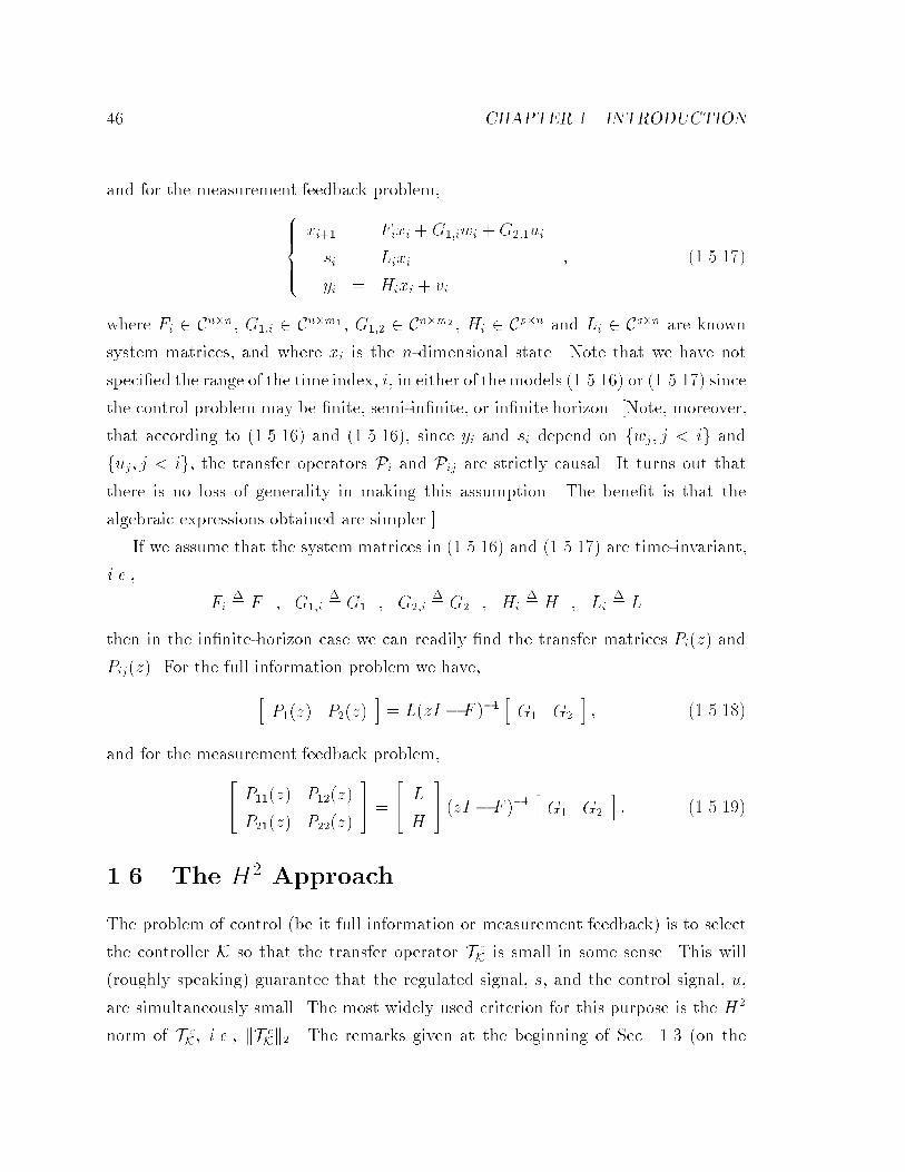
�� CHAPTER �� INTRODUCTION
and for the measurement feedback problem����������
xi�� � Fixi �G��iwi �G���ui
si � Lixi
yi � Hixi � vi
� ��������
where Fi � Cn�n� G��i � Cn�m� � G��� � Cn�m� � Hi � Cp�n and Li � Cq�n are known
system matrices� and where xi is the n�dimensional state� Note that we have not
speci�ed the range of the time index� i� in either of the models �������� or �������� since
the control problem may be �nite� semi�in�nite� or in�nite horizon� �Note� moreover�
that according to �������� and ��������� since yi and si depend on fwj� j � ig and
fuj� j � ig� the transfer operators Pi and Pij are strictly causal� It turns out that
there is no loss of generality in making this assumption� The bene�t is that the
algebraic expressions obtained are simpler��
If we assume that the system matrices in �������� and �������� are time�invariant�
i�e��
Fi�� F � G��i
�� G� � G��i
�� G� � Hi
�� H � Li
�� L
then in the in�nite�horizon case we can readily �nd the transfer matrices Pi�z� and
Pij�z�� For the full information problem we have�
hP��z� P��z�
i� L�zI � F ���
hG� G�
i� ��������
and for the measurement feedback problem��� P���z� P���z�
P���z� P���z�
�� �
�� L
H
�� �zI � F ���
hG� G�
i� ��������
��� The H Approach
The problem of control �be it full information or measurement feedback� is to select
the controller K so that the transfer operator T cK is small in some sense� This will
�roughly speaking� guarantee that the regulated signal� s� and the control signal� u�
are simultaneously small� The most widely used criterion for this purpose is the H�
norm of T cK� i�e�� kT
cKk�� The remarks given at the beginning of Sec� ��� �on the

���� THE H� APPROACH ��
de�nition of the H� norm in the �nite and in�nite�horizon cases� and on the reasons
for the pervasive use of the H� criterion� all apply here as well and will therefore not
be repeated�� Instead we shall comment on the connections with linear�quadratic�
regulator �LQR� and linear�quadratic�Gaussian �LQG� control�
����� Connections to LQR and LQG Control
Consider the �nite�horizon case and the quadratic cost function�
J cN �
NXi��
s�i si �NXi��
u�iui� �������
The above cost function is obviously a measure of how large the regulated and control
signals are and is an indication of how well our control strategy performs� We can� of
course� also write
J cN � ksk
�� � kuk
��� ����� �
Assume now that the fwjg and fvjg are zero�mean� uncorrelated and temporally
white stochastic processes with unit variance� i�e��
E
�� wi
vi
�� h w�
j v�j
i�
�� Im �
� Ip
�� �ij� �������
Then J cN itself will be a random variable� Computing the mean value of J c
N yields� in
the full information case�
EJ cN � E
hs� u�
i �� s
u
�� � E w�T c�
K TcKw � E trace �T c�
K TcKww
�� � �������
and in the measurement feedback case�
EJ cN � E
hs� u�
i�� s
u
�� � E
hw� v�
iT c�K T
cK
�� w
v
��
� E trace
��T c�
K TcK
�� w
v
�� h w� v�
i A �
�������
��An excellent bibliography on developments inH� control until �� � has been complied in MG ���See also the �� � special issue of the IEEE Transactions on Automatic Control devoted to LQGcontrol Ath ���
�� CHAPTER �� INTRODUCTION
In view of �������� we have E
�� w
v
�� h w� v�
i� I� so that in both the full informa�
tion and measurement feedback cases the expected quadratic cost functions become�
E
�NXi��
s�i si �NXi��
u�iui
�� trace �T c�
K TcK� � kT
cKk
��� �������
which is the cost function that H��optimal controllers minimize� Therefore� in the
�nite�horizon case� and under the aforementioned statistical assumptions�H��optimal
controllers minimize an expected quadratic cost function� This is why they are also
referred to as linear least�mean�squares controllers�
Using a similar argument in the in�nite�horizon time�invariant case� it is possible
to show that
E �s�i si � u�iui� ��
�
Z ��
�kTK�e
j��k�Fd� � kTKk��� �������
Therefore� in the in�nite�horizon case� H��optimal controllers also minimize an ex�
pected quadratic cost function�
Remarks�
�a� If� in addition to the aforementioned statistical assumptions� the fwjg and fvjg
are assumed to be jointly Gaussian� then the H��optimal controller is a least�
mean�squares controller �i�e�� we do not need to restrict the controller to being
linear�� H��optimal controllers are therefore often called LQG controllers to
emphasize that �L�� they are linear� �Q�� the cost function is quadratic� and
�G�� the exogenous inputs are Gaussian�
�b� Consider the full information problem where we have state�space structure�
When the driving disturbance is assumed zero� so that the only exogenous
variable is the initial state� x�� it is very easy to see that H��optimal controllers
solve the following �nite and in�nite horizon optimization problems�
minfuig
NXi��
s�i si �NXi��
u�iui and minfuig
�Xi��
s�i si ��Xi��
u�iui� �������
The above problems are referred to as linear quadratic regulator problems� We
shall study them in more detail in Chapter ��

���� THE H� APPROACH ��
����� The Full Information Solution
The solution to the H� full information control problem is well known �see e�g��
�Bro���� �AM��� and �KS� �� and is given in the following Theorem�
Theorem ����� �H��optimal Full Information Controller� The solution to the
problem
mincausal K
�������� P� � P�K
K
���������
�������
is given by
K � ��I � P��P��
����n�I � P�
�P������P�
�P�
o�
��������
where �I�P��P������ and �I�P�
�P������ are found from the dual canonical �maximum�
phase minimum�phase� factorization
I � P��P� � �I � P
��P��
����I � P��P��
���� ��������
and where the notation fAg� denotes the causal part of the transfer operator� A�
In �������� the transfer operator �I�P��P����� is both causal and causally invertible
�hence minimum phase� and the transfer operator �I � P��P����� is both anti�causal
and anti�causally invertible �hence maximum phase�� Note� however� that the fac�
torization �������� is di�erent from the factorization �������� required in the solution
of the H� estimation problem� in the sense that the maximum�phase factor appears
on the left and the minimum�phase factor on the right� rather than vice�versa� For
this reason� we have called Eq� �������� the dual canonical factorization� It should
be remarked that� as with the usual canonical factorization� the dual canonical fac�
torization of a positive�de�nite operator �such as I � P��P�� always exists �see e�g�
�Spe�����GK����� �In the �nite�horizon case �������� is simply the UU� �block upper�
lower triangular� decomposition of the matrix I � P��P���
As mentioned earlier� the full information control problem can be considered to
be the dual of the estimation problem� Although the �nal solution of Eq� ��������
already shows some of this duality� in order to display the duality in a more revealing
fashion let us take the negative conjugate transpose of �������� to write
�K� �nP��P��I � P
��P��
����oa�c�
�I � P��P��
���� ������ �

�� CHAPTER �� INTRODUCTION
where fAga�c� denotes the anticausal part of the operator A� and where we have used
the readily veri�ed identity fAg�� � fA�ga�c�� Inspection of ������ � reveals that by
replacing the anticausal operators �K�� P�� and P
�� with the causal operators K� L
and H� replacing f�ga�c� with f�g�� and replacing the dual canonical factorization
�������� with the usual factorization� one readily obtains the H� estimator of Eq�
�������� Thus the solutions of Theorems ����� and ����� are truly the dual of one
another�
Proof of Theorem ������ The proof is the dual to the proof of Theorem ����� and
will not be repeated here�
����� The Measurement Feedback Solution
In the estimation problems of Secs� ��� and ��� and in the full information control
problem considered so far� the estimators and controllers obtained were both causal
and stable��� This was true even when the underlying transfer operators �L and H
in estimation� P� and P� in control� where causal but unstable� The resulting H�
and H� estimators and full information controllers also lead to causal and stable TK
and T cK� However� as we shall presently see� in the measurement feedback problem
we can no longer guarantee the stability of the causal controller� K� Despite this� the
stability of T cK can still ge guaranteed�
The solution to the H� measurement feedback control problem is given below and�
as mentioned earlier� involves a certain two�step procedure known as the separation
principle�
��Until the present we have deliberately not been very speci�c about the distinction between causaland stable operators� A causal operator is one for which the mapping from future inputs to past andcurrent outputs is zero� i�e�� the output at any given time is only a function of past and current inputs�On the other hand� there are many di�erent notions of stability for linear transfer operators �such asL�� L� and exponential stability�� but they all essentially amount to the fact that if the inputs arebounded �in some sense� then the outputs are also bounded �in some sense�� For example� causaloperators with transfer matrix representations can formally be written as H�z� � H�H�z
��� � � ��However� such operators need not be stable since in such a formal expansion the Hi need not bebounded� L� �or H�� stability� for example� requires that
P�
j trace�H�
jHj� ���
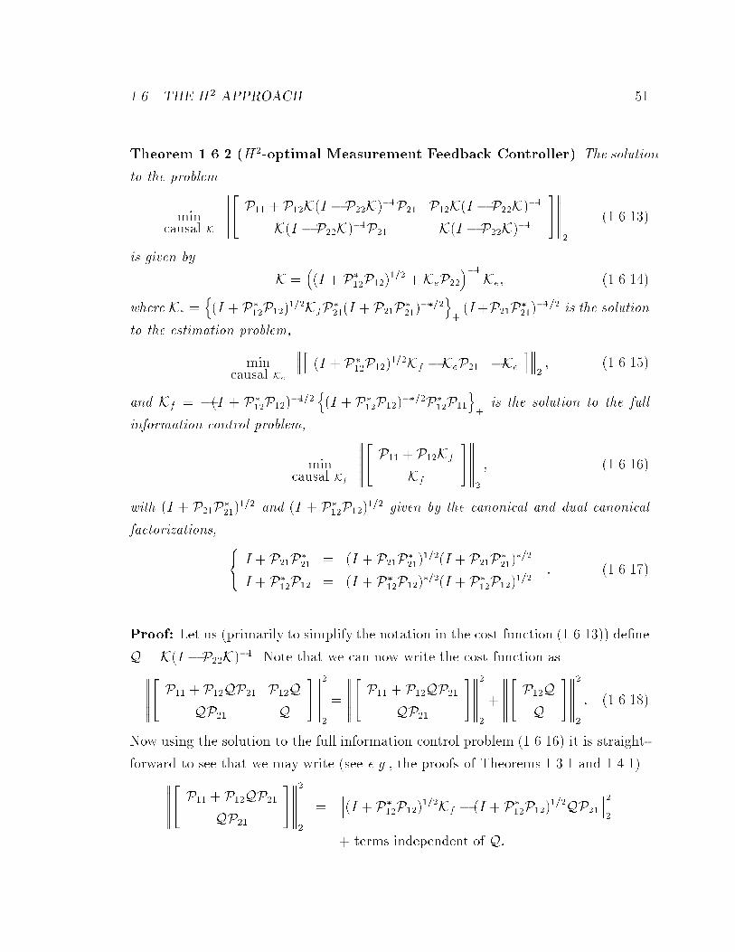
���� THE H� APPROACH ��
Theorem ���� �H��optimal Measurement Feedback Controller� The solution
to the problem
mincausal K
�������� P�� � P��K�I �P��K���P�� P��K�I �P��K���
K�I �P��K���P�� K�I �P��K���
���������
��������
is given by
K ���I � P�
��P������ �KeP��
���Ke� ��������
where Ke �n�I � P�
��P������KfP����I � P��P�
�������
o��I�P��P�
������� is the solution
to the estimation problem�
mincausal Ke
���h �I � P���P������Kf �KeP�� �Ke
i����� ��������
and Kf � ��I � P���P�������
n�I � P�
��P�������P���P��
o�
is the solution to the full
information control problem�
mincausal Kf
�������� P�� � P��Kf
Kf
���������
� ��������
with �I � P��P����
��� and �I � P���P������ given by the canonical and dual canonical
factorizations� ��� I � P��P�
�� � �I � P��P����
����I � P��P����
���
I � P���P�� � �I � P�
��P�������I � P���P������
� ��������
Proof� Let us �primarily to simplify the notation in the cost function ��������� de�ne
Q � K�I �P��K���� Note that we can now write the cost function as�������� P�� � P��QP�� P��Q
QP�� Q
���������
�
�
�������� P�� � P��QP��
QP��
���������
�
�
�������� P��Q
Q
���������
�
� ��������
Now using the solution to the full information control problem �������� it is straight�
forward to see that we may write �see e�g�� the proofs of Theorems ����� and �������������� P�� � P��QP��
QP��
���������
�
�����I � P�
��P������Kf � �I � P
���P���
���QP��
�����
� terms independent of Q�
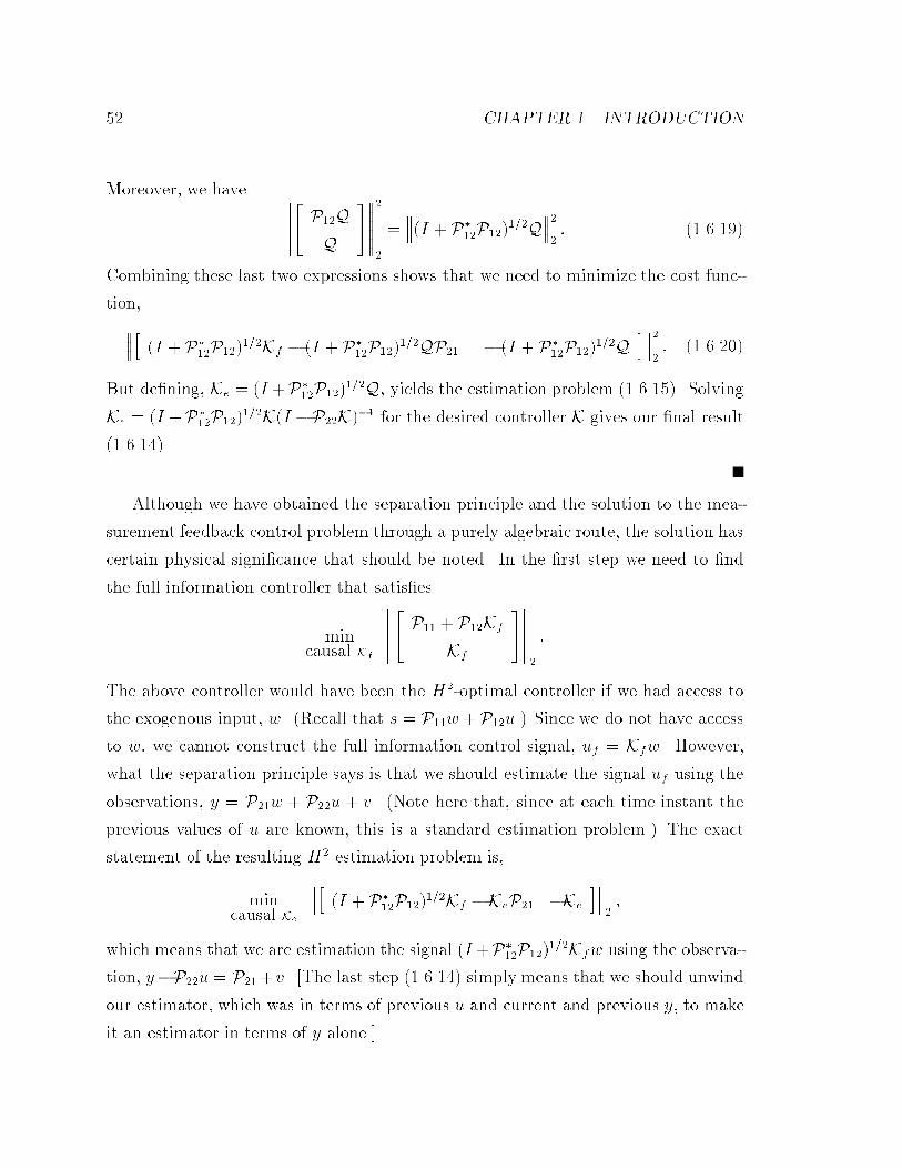
� CHAPTER �� INTRODUCTION
Moreover� we have �������� P��Q
Q
���������
�
�����I � P�
��P������Q
������ ��������
Combining these last two expressions shows that we need to minimize the cost func�
tion�
���h �I � P���P������Kf � �I � P�
��P������QP�� � �I � P���P������Q
i������ ����� ��
But de�ning� Ke � �I �P���P������Q� yields the estimation problem ��������� Solving
Ke � �I �P���P������K�I �P��K��� for the desired controller K gives our �nal result
���������
Although we have obtained the separation principle and the solution to the mea�
surement feedback control problem through a purely algebraic route� the solution has
certain physical signi�cance that should be noted� In the �rst step we need to �nd
the full information controller that satis�es
mincausal Kf
�������� P�� � P��Kf
Kf
���������
�
The above controller would have been the H��optimal controller if we had access to
the exogenous input� w� �Recall that s � P��w�P��u�� Since we do not have access
to w� we cannot construct the full information control signal� uf � Kfw� However�
what the separation principle says is that we should estimate the signal uf using the
observations� y � P��w � P��u � v� �Note here that� since at each time instant the
previous values of u are known� this is a standard estimation problem�� The exact
statement of the resulting H� estimation problem is�
mincausal Ke
���h �I � P���P������Kf �KeP�� �Ke
i�����
which means that we are estimation the signal �I�P���P������Kfw using the observa�
tion� y�P��u � P���v� �The last step �������� simply means that we should unwind
our estimator� which was in terms of previous u and current and previous y� to make
it an estimator in terms of y alone��

���� THE H� APPROACH ��
As a matter of fact� we shall later see that in actually trying to �nd theH��optimal
measurement feedback controller �say� for systems described by state�space models�
it is easier to keep the physical meaning of the separation in mind� rather than to
explicitly use the solution of Theorem ���� �
Finally� we remark once more that the key to the solution of the H� full informa�
tion and measurement feedback control problems is obtained through the canonical
factorization of certain positive de�nite transfer operators�
����� Special Cases
We will now consider the solutions of Theorems ����� and ���� in the cases where the
underlying transfer operators have transfer matrix representations and state�space
structure� We shall� in particular� see that the in the full information problem the
solution is given by a �well known� state feedback law� and that in the measurement
feedback problem one instead uses a feedback based on estimates of the state�
Transfer Matrices � Full Information Case
As noted in Sec� ������ when the underlying transfer operators have transfer matrix
representations we can write��� s�z� � P��z�w�z� � P��z�u�z�
u�z� � K�z�w�z�� ����� ��
Suppose� moreover� that the quadratic cost whose expected value we seek to minimize
is given by
s�iRcsi � u�iQ
cui� ����� �
where Rc � � and Qc � � are given weighting matrices���
Using Theorem ����� the full information controller is given by
K�z� � �N���z�R��c
nN���z���P �
� �z���RcP��z�
o�� ����� ��
�This slight generalization of the problem considered so far is of no signi�cant consequence� Indeedwe can go back to the standard problem by the transformations� �Rc����si � si� �Qc����ui � ui��Rc����P��z�� P��z� and �Rc����P��z�� P��z��

�� CHAPTER �� INTRODUCTION
where N�z� is found from the dual canonical factorization�
Qc � P �� �z
���RcP��z� � N��z���RcN�z�� ����� ��
with N�z� causal and causally invertible� and where Rc is such that we have the
normalization
N�� � Im�� ����� ��
As with the H� estimation problem� the solution requires a �here dual� canonical
spectral factorization� As also was the case there� when the transfer matrices have
state�space structure� viz��
hP��z� P��z�
i� L�zI � F ���
hG� G�
i� ����� ��
then the canonical factorization can be explicitly obtained via the solution of a DARE
�discrete�time algebraic Riccati recursion�� Indeed� if fF�G��Qc����g is stabilizable
and fF� �Rc����Lg is detectable� then N�z� in ����� �� is given by
N�z� � Im��Kc�zI � F ���G� � Kc � R��
c G��P
cF � Rc � Qc �G��P
cG� ����� ��
where P c is the unique positive semide�nite solution to the �dual� DARE���
P c � F �P cF � L�RcL�K�cRcKc� ����� ��
Moreover� P c is such that the matrix�
Fc�� F �G�Kc� ����� ��
is stable� which is in accordance with the fact that the inverse of N�z��
N���z� � Im��Kc�zI � F �G�Kc�
��G� � I �Kc�zI � Fc���G�� ��������
must be causal�
�Note that this DARE is the dual to the DARE ������� given in the solution to the H� estimationproblem�
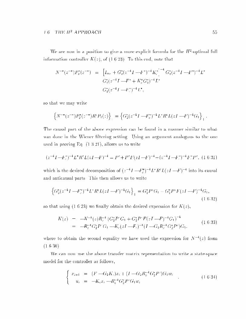
���� THE H� APPROACH ��
We are now in a position to give a more explicit formula for the H��optimal full
information controller K�z�� of ����� ��� To this end� note that
N���z���P �� �z
��� �hIm�
�G���z
��I � F ����K�c
i��G���z
��I � F ����L�
� G���z
��I � F � �K�cG
�����L�
� G���z
��I � F �c �
��L��
so that we may write
nN���z���P �
� �z���RcP��z�
o��nG���z
��I � F �c �
��L�RcL�zI � F ���G�
o��
The causal part of the above expression can be found in a manner similar to what
was done in the Wiener �ltering setting� Using an argument analogous to the one
used in proving Eq� ����� ��� allows us to write
�z��I�F �c ���L�RcL�zI�F ��� � P c�P cF �zI�F �����z��I�F �
c ���F �
c Pc� ��������
which is the desired decomposition of �z��I � F �c �
��L�RcL�zI � F ��� into its causal
and anticausal parts� This then allows us to write
nG���z
��I � F �c �
��L�RcL�zI � F ���G�
o�� G�
�PcG� �G�
�PcF �zI � F ���G��
������ �
so that using ����� �� we �nally obtain the desired expression for K�z��
K�z� � �N���z�R��c �G�
�PcG� �G�
�PcF �zI � F ���G��
��
� �R��c G�
�PcG� �Kc�zI � Fc����I �G�R
��c G�
�Pc�G��
��������
where to obtain the second equality we have used the expression for N���z� from
���������
We can now use the above transfer matrix representation to write a state�space
model for the controller as follows�
��� xi�� � �F �G�Kc�xi � �I �G�R
��c G�
�Pc�G�wi
ui � �Kcxi �R��c G�
�PcG�wi
� ��������

�� CHAPTER �� INTRODUCTION
The reason why we have used the notation xi for the state variable in �������� is
that it really is the state vector for the plant� Indeed using the expression for ui �
�Kcxi �R��c G�
�PcG�wi in the state equation of �������� allows us to write���
� xi�� � Fxi �G�wi �G�ui
ui � �Kcxi �R��c G�
�PcG�wi
� ��������
which shows that xi is the plant�s state vector�
The above solution has an interesting structure and shows that the control signal�
ui� is a function only of the current state� xi� and the current driving disturbance� wi�
This is slightly di�erent from the �now famous� state feedback solution of continuous�
time H� optimal control where the control signal depends only on the current state�
The reason why this di�erence occurs is that �from the outset� we have insisted on
causal controllers� Had we insisted on strictly causal controllers� i�e�� controllers that
only have access to past values of the exogenous input� w� then we would have obtained
a state feedback controller�
Indeed in that case� following similar arguments� one can show that the strictly
causal H��optimal full information controller is given by�
K�z� � �N���z�R��c
nN���z���P �
� �z���RcP��z�
os�c�
� ��������
where the notation fA�z�gs�c� denotes the strictly causal part of the transfer matrix
A�z�� In this case�
nG���z
��I � F �c �
��L�RcL�zI � F ���G�
os�c�� G�
�PcF �zI � F ���G��
from which we conclude
K�z� � Kc�zI � Fc���G�� ��������
which has state�space representation���� xi�� � Fxi �G�wi �G�ui
ui � �Kcxi� ��������
This last expression is the wellknown state feedback law of H��optimal control�
It is useful to summarize the results obtained so far in the following Theorem�

���� THE H� APPROACH ��
Theorem ����� �Innite�Horizon H��optimal Full Information Controller� �a� The
solution to the problem
mincausal K�z�
�������� R��� �P��z� � P��z�K�z��
Q���K�z�
���������
� ��������
is given by
K�z� � �N���z�R��c
nN���z���P �
� �z���RcP��z�
o�� ��������
where N�z� is found from the dual canonical spectral factorization
Qc � P �� �z
���RcP��z� � N��z���RcN�z��
with N�z� causal and causally invertible� and N�� � Im��
When P��z� and P��z� have state�space structure�
hP��z� P��z�
i� L�zI � F ���
hG� G�
i�
with fF�G��Qc����g stabilizable and fF� �Rc����Lg detectable� then
K�z� � �R��c G�
�PcG� �Kc�zI � Fc�
���I �G�R��c G�
�Pc�G�� ��������
where Kc � R��c G�
�PcF � Rc � Qc �G�
�PcG�� and P c the unique positive semide�nite
solution of the DARE�
P c � F �PF � L�RcL�K�cRcKc�
In this case� the control signal� ui� is given by
ui � �Kcxi �R��c G�
�PcG�wi� ������ �
where xi is the state variable satisfying� xi�� � Fxi �G�wi �G�ui�
�b� The solution to the problem
minstrictly causal K�z�
�������� R��� �P��z� � P��z�K�z��
Q���K�z�
���������
� ��������
is given by
K�z� � N���z�R��c
nN���z���P �
� �z���RcP��z�
os�c�
� ��������

�� CHAPTER �� INTRODUCTION
When P��z� and P��z� have the state�space structure of part �a�� then the H��optimal
control signal is given by the state feedback law�
ui � �Kcxi� ��������
where Kc is as in part �a��
Transfer Matrices � Measurement Feedback Case
In the measurement feedback case� the underlying transfer operators have transfer
matrix representations of the form����������
s�z� � P���z�w�z� � P���z�u�z�
y�z� � P���z�w�z� � P���z�u�z� � v�z�
u�z� � K�z�y�z�
� ��������
We shall once more assume that the cost function �whose expected value is to be
minimized� is given by
s�iRcsi � u�iQ
cu� ��������
and that the fwi� vig are zero�mean stationary stochastic processes such that
E
�� wi
vi
�� h w�
j v�j
i�
�� Q �
� R
�� �ij� ��������
The H��optimal measurement feedback controller can now be found using the
recipe of Theorem ���� � However� for brevity we shall not do so here� since the
solution is simply the restatement of Theorem ���� when transfer operators are re�
placed by transfer matrices� Instead we shall focus on the case where the Pij�z� have
state�space structure of the form�� P���z� P���z�
P���z� P���z�
�� �
�� L
H
�� �zI � F ���
hG� G�
i� ��������
As we have just seen� the full information controller is given by
uf�i � �Kcxi �R��c G�
�PcG�wi�

���� THE H� APPROACH ��
Now according to Theorem ���� the H��optimal measurement feedback control signal
is simply the H� estimate of uf�i given the observations� fyj� j � ig� Thus�
ui � �Kc�xiji �R��c G�
�PcG� �wiji� ��������
where �xiji and �wiji denote the linear least�mean�squares estimates of xi and wi given
fyj� j � ig��� But since the fyj� j � ig are independent of wi �since P���z� � H�zI �
F ���G� is strictly causal and the fwjg are white�� we have �wiji � �� so that
ui � �Kc�xiji� ��������
Since the observations� yi� satisfy the state�space model���� xi�� � Fxi �G�wi �G�ui
yi � Hxi � vi������ �
the state estimates can be readily found from the Wiener �lter recursions �see Theo�
rem ���� �� ��� �xi�� � �F �KpH��xi �Kpyi �G�ui
�xiji � �I � PH�R��e H��xi � PH�R��
e yi� ��������
where Kp � FPH�R��e � Re � R � HPH�� P is the unique positive semide�nite
solution to the DARE�
P � FPF � �G�QG�� �KpReK
�p � ��������
and where we have used the fact that at time i� the fuj� j � ig are known� Using�
ui � �Kc�xiji The above state�space model may be rewritten as��� �xi�� � �F �KpH �G�Kc�I � PH�R��
e H�� �xi � �Kp �G�KcPH�R��
e �yi
ui � �Kc�I � PH�R��e H��xi �KcPH
�R��e yi
�
��������
from which we infer that optimal controller is
K�z� � �Kc
hPH�R��
e � �I � PH�R��e H��zI � Fm�
���Kp �G�KcPH�R��
e �i�
��������
��Note that we have used the fact that inH� estimation the best estimate of any linear combinationof the state is simply that linear combination of the best state estimate� We saw that this was notthe case in H� estimation� a fact that will have certain rami�cations for H� control�
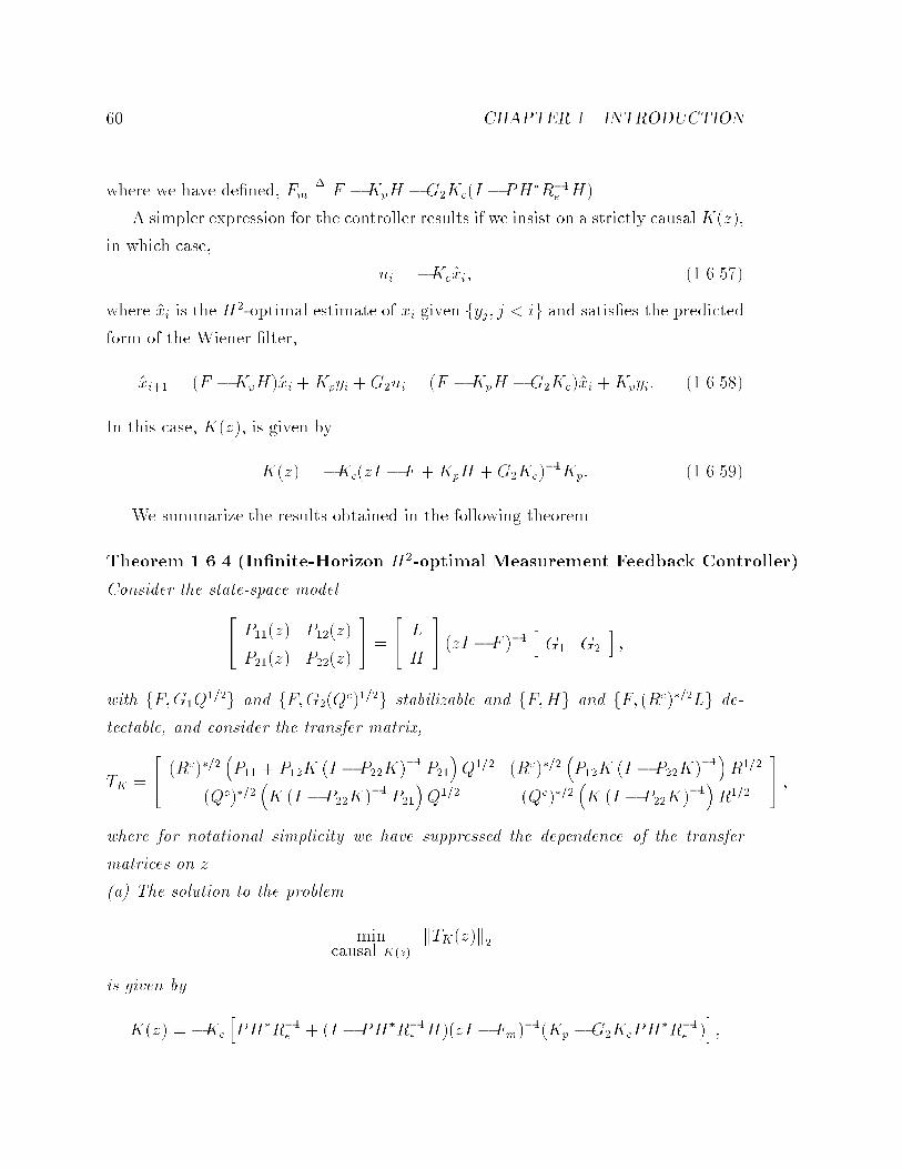
�� CHAPTER �� INTRODUCTION
where we have de�ned� Fm�� F �KpH �G�Kc�I � PH�R��
e H��
A simpler expression for the controller results if we insist on a strictly causal K�z��
in which case�
ui � �Kc�xi� ��������
where �xi is the H��optimal estimate of xi given fyj� j � ig and satis�es the predicted
form of the Wiener �lter�
�xi�� � �F �KpH��xi �Kpyi �G�ui � �F �KpH �G�Kc��xi �Kpyi� ��������
In this case� K�z�� is given by
K�z� � �Kc�zI � F �KpH �G�Kc���Kp� ��������
We summarize the results obtained in the following theorem�
Theorem ����� �Innite�Horizon H��optimal Measurement Feedback Controller�
Consider the state�space model�� P���z� P���z�
P���z� P���z�
�� �
�� L
H
�� �zI � F ���
hG� G�
i�
with fF�G�Q���g and fF�G��Qc����g stabilizable and fF�Hg and fF� �Rc����Lg de�
tectable� and consider the transfer matrix�
TK �
�� �Rc����
�P�� � P��K �I � P��K�
�� P���Q��� �Rc����
�P��K �I � P��K�
���R���
�Qc�����K �I � P��K�
�� P���Q��� �Qc����
�K �I � P��K�
���R���
�� �
where for notational simplicity we have suppressed the dependence of the transfer
matrices on z�
�a� The solution to the problem
mincausal K�z�
kTK�z�k�
is given by
K�z� � �Kc
hPH�R��
e � �I � PH�R��e H��zI � Fm�
���Kp �G�KcPH�R��
e �i�
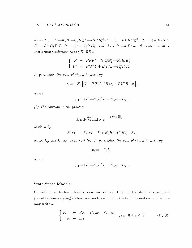
���� THE H� APPROACH ��
where Fm � F �KpH �G�Kc�I � PH�R��e H�� Kp � FPH�R��
e � Re � R�HPH��
Kc � R��c G�
�PcF � Rc � Qc � G�
�PcG�� and where P and P c are the unique positive
semide�nite solutions to the DARE�s���� P � FPF � �G�QG
�� �KpReK
�p
P c � F �P cF � L�RcL �K�cRcKc
�
In particular� the control signal is given by
ui � �Kc
h�I � PH�R��
e H��xi � PH�R��e yi
i�
where
�xi�� � �F �KpH��xi �Kpyi �G�ui�
�b� The solution to the problem
minstrictly causal K�z�
kTK�z�k�
is given by
K�z� � �Kc�zI � F �KpH �G�Kc���Kp�
where Kp and Kc are as in part �a�� In particular� the control signal is given by
ui � �Kc�xi�
where
�xi�� � �F �KpH��xi �Kpyi �G�ui�
State�Space Models
Consider now the �nite horizon case and suppose that the transfer operators have
�possibly time�varying� state�space models which for the full information problem we
may write as ��� xi�� � Fixi �G��iwi �G���ui
si � Lixi� x�� � � i � N ��������
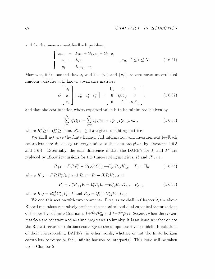
� CHAPTER �� INTRODUCTION
and for the measurement feedback problem����������xi�� � Fixi �G��iwi �G���ui
si � Lixi
yi � Hixi � vi
� x�� � � i � N� ��������
Moreover� it is assumed that x� and the fuig and fvig are zero�mean uncorrelated
random variables with known covariance matrices
E
��x�
ui
vi
��hx�� u�j v�j
i�
�� � � �
� Qi�ij �
� � Ri�ij
�� � ������ �
and that the cost function whose expected value is to be minimized is given by
NXi��
s�iRcisi �
NXi��
u�iQciui � x�N��P
cN��xN��� ��������
where Rci � �� Q
ci � � and P
cN�� � � are given weighting matrices�
We shall not give the �nite horizon full information and measurement feedback
controllers here since they are very similar to the solutions given by Theorems �����
and ������ Essentially� the only di�erence is that the DARE�s for P and P c are
replaced by Riccati recursions for the time�varying matrices� Pi and P ci � i�e��
Pi�� � FiPiF�i �G��iQiG
���i �Kp�iRe�iK
�p�i� P� � � ��������
where Kp�i � FiPiH�i R
��e�i and Re�i � Ri �HiPiH
�i � and
P ci � F �
i Pci��Fi � L�iR
ciLi �K�
c�iRc�iKc�i� P cN�� ��������
where Kc�i � R��c�iG
���iP
ci��F and Rc�i � Qc
i �G���iP
ci��G��i�
We end this section with two comments� First� as we shall in Chapter � the above
Riccati recursions recursively perform the canonical and dual canonical factorizations
of the positive de�nite Gramians� I�P��P��� and I�P
���P��� Second� when the system
matrices are constant and as time progresses to in�nity� it is an issue whether or not
the Riccati recursion solutions converge to the unique positive semide�nite solutions
of their corresponding DARE�s �in other words� whether or not the �nite horizon
controllers converge to their in�nite horizon counterparts�� This issue will be taken
up in Chapter ��

���� THE H� APPROACH ��
����� The Question of Robustness
As we have just seen� under suitable stochastic assumptions� such as �jointly Gaussian�
uncorrelated disturbances with known �rst and second order statistics� H��optimal
controllers have certain desirable optimality properties� namely that they minimize
the expected value of a certain quadratic cost�
In practice� however� we may not always know the statistics of the disturbances�
We also often do not know the exact models that generate our signals of interest�
Therefore� as was the case with H� estimation� we cannot always guarantee the va�
lidity of the assumptions required of H� controllers� The natural question that arises
in this regard is what the performance of such controllers will be if the assumptions
on the disturbances are violated� or if there are modeling errors in our model so that
the disturbances must include the modeling errors! In other words�
� is it possible that small disturbances and modeling errors may lead to large
costs�
Intuitively� a non�robust controller is one for which the above is true� i�e�� one for
which small disturbances may force us to incur large costs� whereas a robust controller
is one for which small disturbances always result in small costs�
In the H� framework to robust control the costs �both the objective cost and
the cost associated with the disturbances� are quadratic�� forms constructed from
the signals� and the goal is to come up with controllers that minimize �or in the
suboptimal case� bound� the maximumgain from the disturbance cost to the objective
cost� This will guarantee that if the disturbances are small� i�e�� if their associated
cost is small� then the objective cost will be as small as possible� no matter what
the disturbances are� The robustness of H� controllers� with respect to modeling
errors and disturbance variation� follows from the fact that the maximum gain is
minimized over all possible disturbances� However� since they make no assumption
about the disturbances and have to accommodate for all conceivable ones� they may
be over�conservative�
Although the aforementioned motivation for H� control is an important one�
��Other approaches to robust control di�er in the de�nition of the cost� In l� control the cost usedis related to the peak value of the signals� DP � and DDB����

�� CHAPTER �� INTRODUCTION
historically� the main motivation for its introduction was somewhat di�erent and is
related to what is now called the robust stabilization problem� �See the pioneering
paper �Zam��� for the initial motivation of H� control and the textbooks �Fra����
�GL��� and �ZDG��� for further properties and related topics�� To understand the
robust stabilization problem�� consider the feedback structure of Fig� ����
D
y i
s iA12
A22
A11
A21u i
wi
u yi i
P
Figure ���� A plant with modeling error�
Suppose that we have a plant� P� that can be represented by a known nominal
plant� A �
�� A�� A��
A�� A��
��� along with an unknown plant� D� that are connected in a
feedback form� In this setting A represents that part of the plant model that we are
aware of� and D represents the modeling errors� Although the uncertainty model� D�
is unknown we shall assume that it is $small� �in a sense to be de�ned shortly��
As depicted in Fig� ���� the objective here is to design a controller� K� that
stabilizes P �for all small uncertainty D�� Since we know the nominal plant� we can
always design a controller that stabilizes it �indeed our ultimate design must also
stabilize A since it corresponds to the special case� D � ��� say� an H� controller�
However� it is not in general clear how robust such a control strategy would be to the
uncertainty� D� In other words� is it possible that $small� modeling errors �which in
practice are inevitable� may unstabilize the composite plant!
To answer this question� let us persist with some choice of controller� K� and
represent the composite plant as the feedback connection of the uncertainty� D� and
��See also San � for what seems to be the �rst analysis of this problem�
���� THE H� APPROACH ��
K
D
AA
AA21
11 12
22 yu
w si
i
i
i
D
A sw (K) sw ii
Figure ���� The robust stabilization problem�
the known plant�
Asw�K� � A�� �A��K�I �A��K���A��� ��������
Now the composite plant will be input�output stable in some given norm� k � k� if�
according to the small gain theorem �see e�g�� �Wil��a�� �DV����� we have
kDAsw�K�k � �� ��������
But if we choose a submultiplicative norm� such as the H� norm��� k � k�� the
composite plant will be stable if�
kDk� � kAsw�K�k� � �� ��������
Suppose now that we know that D is small in the sense that
kDk� � �� ��������
Then we will have stability if�
kAsw�K�k� ��
��� � ��������
Indeed� we even have the following stronger statement� If �������� is not satis�ed�
then there exists some norm�bounded uncertainty� D with kDk� � �� such that
��We could also use other submultiplicative norms such as the l� norm�

�� CHAPTER �� INTRODUCTION
the composite plant is unstable� Therefore condition� �������� is the necessary and
sucient condition for input�output stability of the composite plant for all model
uncertainties� kDk� � ��
Thus we are lead to the design of a controller that bounds the H� norm from the
exogenous input w to the regulated output s for the nominal plant� We will study
the H� control problem in a more general setting �one which subsumes the above
problem� that is motivated by bounding the maximum gain from the disturbance cost
to the objective cost�
��� The H Approach
In this section we brie�y describe theH� approach to robust control� �For alternative
presentations and derivations see the textbooks �Fra���� �BB���� �GL���� �ZDG��� and
the references therein��
Returning to the control problems of Sec� ���� we recall that a useful representation
for any control strategy K is� in the full information problem� the transfer operator�
T cK �
�� P� � P�K
K
�� �
that maps the exogenous input fwjg to the regulated and control signals fsjg and
fujg� and� in the measurement feedback problem� the transfer operator�
T cK �
�� P�� � P��K�I �P��K�
��P�� P��K�I �P��K���
K�I �P��K���P�� K�I �P��K���
�� �
that maps the exogenous inputs fwjg and fvjg to the regulated and control signals
fsjg and fujg�
In either case� for any choice of controllerK� and for any exogenous input sequence�
we can readily compute the energy gain from the exogenous inputs to the regulated
and control signals� For example in the measurement feedback problem�
ksk�� � kuk��
kwk�� � kvk��
�
������T cK
�� w
v
���������
�
kwk�� � kvk��
� �������

��� THE H� APPROACH ��
Clearly� the ratio in ������� depends on the particular choice of the input disturbances
w and v� As in the H� estimation problem� to remove this dependency� and to ensure
robustness with respect to disturbance variation� we consider the largest energy gain
in ������� over all possible w and v� i�e�� the H� norm of a transfer operator T cK� This
leads us to the following problem�
Problem �� �� �Optimal H� Control Problems� �a� Full Information Problem�
Find a causal controller K that minimizes the H� norm of the transfer operator T cK
that maps the exogenous input fwjg to the regulated and control signals� fsjg and
fujg� i�e� � �nd a causal K that satis�es�
infKkT c
Kk� � infK
�������� P� � P�K
K
���������
� ����� �
Moreover �nd the resulting opt � infK kT cKk��
�b� Measurement Feedback Problem� Find a causal controller K that minimizes the
H� norm of the transfer operator T cK that maps the exogenous inputs fwjg and fvjg
to the regulated and control signals� fsjg and fujg� i�e� � �nd a causal K that satis�es�
infKkT c
Kk� � infK
�������� P�� � P��K�I �P��K���P�� P��K�I �P��K���
K�I �P��K���P�� K�I �P��K�
��
���������
� �������
Moreover �nd the resulting opt � infK kTcKk��
�Note� once more� that in the above problem statement we are purposefully am�
biguous as to whether we are considering the �nite horizon or �semi�in�nite horizon
case��
The minimax nature of H� optimal controllers is evident from ����� � and ��������
Thus theH� control problem can be regarded as a game where nature �the opponent�
has access to the unknown exogenous inputs w and v and we have choice of the causal
controller K� Note� moreover� that although H� optimal controllers are robust with
respect to disturbance variation they may be over conservative �as no assumption is
made regarding the disturbances��
There are very few case where a closed�form solution to the optimal H� problem
of Prob� ����� can be found� and in general one resorts to the following suboptimal
solution�

�� CHAPTER �� INTRODUCTION
Problem �� � �Suboptimal H� Control Problems� �a� Full Information Prob�
lem� Given a �� �nd a causal estimator K that guarantees
kT cKk� �
�������� P� � P�K
K
���������
� � �������
This clearly requires checking whether is an achievable bound�
�b� Measurement Feedback Problem� Given a �� �nd a causal estimator K that
guarantees
kT cKk� �
�������� P�� � P��K�I �P��K�
��P�� P��K�I �P��K���
K�I �P��K���P�� K�I �P��K���
���������
� � �������
This clearly requires checking whether is an achievable bound�
����� The Full Information Solution
The solution to the full information H� control problem is essentially the dual to the
H� estimation problem of Theorem ����� and is given below�
Theorem �� �� �H� Suboptimal Full Information Controllers� A causal con�
troller� K that achieves �������� P� � P�K
K
���������
�
exists if� and only if� there exists a dual canonical factorization of the form�� I � P�
�P� P��P�
P��P� ��I � P�
�P�
�� �
�� L��� L���
L��� L���
���� I �
� �I
���� L�� L��
L�� L��
�� �
with
�� L�� L��
L�� L��
�� and L�� causal and causally invertible� and L�� strictly causal� If
this is the case� then all possible H� estimators of level are given by
K � �L�� �QL������QL�� � L���� �������
where Q is any causal and strictly contractive operator� An important choice results
from taking Q � �� so that
Kcen � �L���� L��� �������

��� THE H� APPROACH ��
which is the so�called central controller�
Proof� The proof is the dual to the proof of Theorem ����� and will not be repeated
here�
Comparing the results of Theorems ����� and ����� reveals the duality between
H� estimation and H� full information control� We shall not comment on this
duality here �other than� perhaps� noting the replacement of an inde�nite canonical
factorization with a dual one�� and shall instead close this section with a remark on
the maximum entropy property of the central full information controller�
Corollary �� �� �Maximum Entropy Property of Central Solution� The so�
lution to the problem
maxcausal K
log deth�I � T c�
K TcK
i�������
is given by the central controller�
Kcen � �L���� L��� �������
����� The Measurement Feedback Solution
The solution to the H� measurement feedback control problem is given below and�
as mentioned earlier� involves a certain separation principle� The separation principle
for H� control was �rst derived in �DGKF��� and is essentially the same as the
separation principle of risk�sensitive control �see �Whi����� although the form given
below somewhat di�ers from those of �DGKF��� and �Whi���� We should also remark
that the H� separation principle is di�erent from its H� counterpart since the H�
full information control problem� and the H� estimation problem� that the H�
measurement feedback problem breaks into are no longer decoupled� We will have
more to say about this in a moment� We also note that� as in the H� case� we can no
longer guarantee the stability of the controller� Moreover� for notational simplicity
we have taken � ��

�� CHAPTER �� INTRODUCTION
Theorem �� � �H� Suboptimal Measurement Feedback Controllers� A causal
controller K that achieves�������� P�� � P��K�I �P��K���P�� P��K�I �P��K���
K�I �P��K���P�� K�I �P��K���
���������
� � ��������
exists if� and only if� the following two conditions are satis�ed�
�i� The full information control problem��������� P�� � P��Kf
Kf
���������
� � ��������
has a causal solution� Kf � In other words� there exists the dual canonical fac�
torization��� I � P�
��P�� P���P��
P���P�� �I � P�
��P��
�� �
�� L��� L���
L��� L���
���� I �
� �I
���� L�� L��
L�� L��
�� �
������ �
with
�� L�� L��
L�� L��
�� and L�� causal and causally invertible� and L�� strictly causal�
�ii� The estimation problem�
���h L��L���� �KeP��L
���� �Ke
i����� � ��������
has a causal solution� Ke� where the Lij are as in part �i�� In other words� there
exists the canonical factorization��� I � P��L
���� L
���� P
��� P��L
���� L
���� L
���
L��L���� L
���� P
��� �I � L��L
���� L
���� L
���
�� �
�� Le
�� Le��
Le�� Le
��
���� I �
� �I
���� Le�
�� Le���
Le��� Le�
��
��
��������
with
�� Le
�� Le��
Le�� Le
��
�� and Le
�� causal and causally invertible� and Le�� strictly causal�
If this is the case� then all possible measurement feedback H� controllers are given
by�
K � �I �QP�����Q� ��������

��� THE H� APPROACH ��
where
Q � �Ke
hL�� � �L�� �KeP���L
���� L��
i��� ��������
and Ke is the solution to the estimation problem ������ � which is parametrized by
Ke � �Le��S � L
e����L
e�� � L
e��S�
��� ��������
with S any causal and strictly contractive operator� The so�called central controller�
Kcen results from the choice S � � and corresponds to Ke�cen � �Le���L
e���
���
Proof� Recall the de�ning relations���������
s � P��w � P��u
y � P��w � P��u� v
u � Ky
so that we may write� u � QP��u�Qv� with Q � K�I�P��K���� Now the condition
�������� is satis�ed if� and only if� for all u and v in h��
ksk�� � kuk��
kwk�� � kvk��
� � � ksk�� � kuk�� � kwk
�� � kvk
�� � �� ��������
De�ning� J�� ksk�� � kuk
�� � kwk
�� � kvk
��� we may write�
J � kP��w � P��uk�� � kuk
�� � kwk
�� � kvk
��
�hu� w�
i �� I � P���P�� P�
��P��
P���P�� ��I � P�
��P��
���� u
w
��� kvk��
�hu� w�
i �� L��� L���
L��� L���
���� I �
� �I
���� L�� L��
L�� L��
���� u
w
��� kvk��
� kL��u� L��wk�� � kL��u� L��wk
�� � kvk
�� � ��
where in the third step we have used the obvious fact that if a measurement feedback
controller exists� if� and only if� a full information one does� in which case dual
canonical factorization can be performed� But this last inequality implies�
kL��u� L��wk��kL��u� L��wk�� � kvk
��
� ��
� CHAPTER �� INTRODUCTION
We can now conclude that a measurement feedback controller exists if� and only if�
K can be chosen such that� ���T baK
��� � �� ��������
where T baK is the transfer operator that maps the signals b and v to the signal a� i�e��
T baK �
�� b
v
��� a� ����� ��
where we have de�ned� ��� a � L��u� L��w
b � L��u� L��w����� ��
Let us now identify T baK � To this end� note that�
� a
b
�� �
�� L�� L��
L�� L��
���� u
w
��
�
�� L�� L��
L�� L��
���� QP�� Q
I �
���� w
v
��
�
�� L��QP�� � L�� L��Q
L��QP�� � L�� L��Q
���� w
v
�� �
Solving for w from the second of the above set of equations yields�
w � �L��QP�� � L�����b� �L��QP�� � L���
��L��Qv�
Plugging the above expression into the equation a � �L��QP�� � L���w � L��Qv
allows us to obtain
T baK �
hA� A�
i� ����� �
where the entries of T baK are given by
��� A� � �L��QP�� � L����L��QP�� � L�����
A� � ��L��QP�� � L����L��QP�� � L�����L��Q� L��Q� ����� ��
As given above� the dependence of T baK on Q seems quite complicated and it does
not appear clear how to choose Q �and hence K� to make T baK a strict contraction�

��� THE H� APPROACH ��
However� let us persist and attempt to simplify the entries of T baK � Indeed�
A� � L��Qh�P���L��QP�� � L���
��L��Q� Ii� L���L��QP�� � L���
��L��Q
� L��QhI � P��L
���� L��Q
i��� L��L
���� �I � L��QP��L
���� �L��Q
� L��Q�I � P��L���� L��Q�
�� � L��L���� L��Q�I � P��L
���� L��Q�
��
� �L�� � L��L���� L���Q�I � P��L
���� L��Q�
��
�� �Ke�
Likewise�
A� � L��QP���L��QP�� � L����� � L���L��QP�� � L���
��
� L��QP���I � L���� L��QP���
��L���� � L���I � L���� L��QP���
��L����
� L��Q�I � P��L���� L��Q�
��P��L���� � L���I � L
���� L��QP���
��L����
� �KeP��L���� � L��L
���� L��Q�I � P��L
���� L��Q�
��P��L���� � L���I � L
���� L��QP���
��L����
� �KeP��L���� � L��L
���� L��QP���I � L
���� L��QP���
��L���� � L���I � L���� L��QP���
��L����
� �KeP��L���� � L��
hL���� L��QP��� I
i�I � L���� L��QP���
��L����
� �KeP��L���� � L��L
���� �
Thus we have shown�
T baK �
hL��L
���� �KeP��L
���� �Ke
i� ����� ��
In other words� the measurement feedback problem has a solution if� and only if� Ke
can be chosen such that T baK is a strict contraction� But this is simply the estima�
tion problem ��������� Finally� we note that solving Ke � �L�� � L��L���� L���Q�I �
P��L���� L��Q��� for Q� and solving Q � K�I � P��K��� for K� yields the desired
results �������� and ���������
A few remarks on the above result are in order� Note that the separation principle
obtained states that to solve the problem we �rst need to solve the full information
control problem� �������� P�� � P��Kf
Kf
���������
� � ����� ��

�� CHAPTER �� INTRODUCTION
and then the estimation problem�
���h L��L���� �KeP��L
���� �Ke
i����� � ����� ��
Note� however� that� unlike the H� case� the above two problems are coupled� since
the estimation problem involves quantities that have to be found from the full infor�
mation problem� As a matter of fact� not only does the solution to the estimation
problem depend on the full information controller� but the actual condition for the
existence of the estimator depends on it as well� �This dependence occurs through the
transfer operators L�� and L�� which are in turn determined by P�� and P���� This
is unlike the H� problem where the separation principle completely decouples the
full information and estimation problems� �There it was neither necessary to decide
on the noise covariances before designing the full information controller� nor on the
control objectives before designing the optimal estimator��
As we shall shortly see� in the state�space case� the coupling between the full
information control and estimation problems is exempli�ed by the fact that their
corresponding DARE�s �or Riccati recursions in the �nite�horizon case� are coupled�
This is as opposed to the H� case where the two Riccati equations are independent
of one another�
Referring to the estimation problem ����� �� shows that the estimatorKe estimates
the output of the system� L��L���� � using noisy observations of the output of the system
P��L���� �see Sec� �� �� However� we shall later see that in actually trying to �nd
the H� measurement feedback controller �say� for systems described by state�space
models� it is much easier to keep the physical meaning of the separation in mind
�such as identifying the signals a and b in the above proof�� rather than to explicitly
use the solution of Theorem ���� �
Finally� it should also be noted that� in the measurement feedback case� the central
solution has the maximum entropy property of
maxcausal K
log deth�I � T c�
K TcK
i� ����� ��

��� THE H� APPROACH ��
����� Special Cases
The general solutions presented so far subsume both the �nite and in�nite horizon
cases� We now brie�y present these�
The Innite Horizon Case
Let us �rst begin with the full information problem for which we have the following
result�
Theorem �� �� �Innite Horizon H� Full Information Controller� �a� A causal
controller� K�z�� that achieves�������� P��z� � P��z�K�z�
K�z�
���������
� �
exists if� and only if� there exists a dual canonical factorization of the form�� Im�
� P��z�P �� �z
��� P��z�P �� �z
���
P��z�P �� �z
��� ��Im�� P��z�P �
� �z���
�� �
�� L����z
��� L����z���
L����z��� L����z
���
���� Im�
�
� �Im�
���� L���z� L���z�
L���z� L���z�
�� �
����� ��
with
�� L���z� L���z�
L���z� L���z�
�� and L���z� minimum phase and proper� and L���z� causal
and strictly proper� If this is the case� then all possible H� full information controllers
of level are given by
K�z� � �L���z��Q�z�L���z���� �Q�z�L���z�� L���
�� � ����� ��
where Q�z� is any causal and strictly contractive transfer matrix� i�e��Q�ej��Q��ej�� �
I� � � ��� ��� The central �lter results from the choice Q�z� � �� so that
Kcen�z� � �L���� �z�L���z�� ��������
�b� Assume that P��z� and P��z� have state�space structure�
hP��z� P��z�
i� L�zI � F ���
hG� G�
i�
�� CHAPTER �� INTRODUCTION
with fF�G�g stabilizable and fF�Lg detectable� Then a solution to the full information
H� control problem with level exists if� and only if� there exists a solution to the
�dual� DARE
P c � F �P cF � L�L�K�cRcKc� ��������
with
Kc � R��c
�� G�
�
G��
��P cF and Rc �
�� Im�
�
� ��Im�
���
�� G�
�
G��
��P c
hG� G�
i������ �
such that
�i� Fc�� F �
hG� G�
iKc is stable�
�ii� Rc and
�� Im�
�
� ��Im�
�� have the same inertia�
If this is the case� then the Lij�z� in the dual canonical factorization �������� are
given by
�� L���z� L���z�
L���z� L���z�
�� �
�� �Im�
�G��P
cG����� �Im��G�
�PcG������G�
�PcG�
� ��Im��G�
�Pc�I �G�G
��P
c���G�����
���
���� Im�
�
� Im�
���Kc�zI � F ���
hG� G�
i A � ��������
In particular� de�ning RGc�� Im�
�G��P
cG�� we have
��� L���z� � R
���Gc
hIm�
�R��GcG
��P
cF �zI � F ���G�
iL���z� � R
���Gc
hR��GcG
��P
cG� �R��GcG
��P
cF �zI � F ���G�
i � ��������
so that
Kcen�z� � �R��GcG
��P
cG� �R��GcG
��P
cF �zI � F�����I �G�R
��GcG
��P
c�G�� ��������
where F��� F �G�R
��GcG
��P
cF �
��� THE H� APPROACH ��
Proof� The proof is the dual of the proof of Theorem ���� and will not be repeated
here�
Remarks�
�i� It is straightforward to give state�space representations for the central controller
��������� Indeed we have
��� xi�� � F�xi � �I �G�R
��GcG
��P
c�G�wi
ui � �R��GcG
��P
cFxi �R��GcG
��P
cG�wi
� ��������
where we have denoted the state variable by xi� since it really is the state of
the original state�space model� To see why� we can use the formulas F� �
F �G�R��GcG
��P
cF and ui � �R��GcG
��P
cFxi�R��GcG
��P
cG�wi in the above state
equation to write�
��� xi�� � Fxi �G�wi �G�ui
ui � �R��GcG
��P
cFxi �R��GcG
��P
cG�wi
� ��������
which is our desired result�
The above controller shows that the full information control signal is a function
only of the current state xi and the current exogenous input� wi�� This is
somewhat di�erent from the state�feedback law that occurs in continuous�time
H� control� The reason is that we have insisted on causal controllers� Had we
sought strictly causal controllers we would have obtained a state feedback law
�for the central solution�� as we now �very� brie�y describe�
�ii� The solution to the problem of �nding a strictly causal full information controller
that achieves� �������� P��z� � P��z�K�z�
K�z�
���������
� �
��The above statement is only true of the central controller� Other full informationH� controllers�as parametrized by ��� ����� need not be so�

�� CHAPTER �� INTRODUCTION
is exactly the same as the solution of Theorem ����� part �a� with the exception
that� in the dual canonical factorization ����� ��� instead of having L���z� being
strictly proper we require that L���z� be strictly proper�
When we have state�space structure� the only di�erence in the existence condi�
tion is that condition �ii� should be replaced by�
��Im��G�
�PcG� � � and Im�
�G��P
c�I � ��G�G��P
c���G� �� ��������
In this case� the Lij�z� are given by��� L���z� L���z�
L���z� L���z�
�� �
�� �
Im�� G�
�Pc�I � ���G�G
��P
c���G�����
�
G��P
cG����Im�
�G��P
cG������ ���Im�
�G��P
cG�����
���
���� Im�
�
� Im�
���Kc�zI � F ���
hG� G�
i A � ������
The above expression allows us to �nd the central solutionK�z� � �L���z���L���z��
which turns out to be�
Kcen�z� � �Kc�zI � F �G��Kc�
��G�� ��������
where
�Kc � �Im��G�
��P cG��
��G���P cF and �P c � P c�P cG���
�Im��G�
�PcG��
��G��P
c�
��������
The above central solution can be shown to have the following state�space model�
��� xi�� � Fxi �G�wi � G�ui
ui � �Kcxi� ������ �
which is� of course� a state�feedback control law�
�iii� Note� once more� the surprising similarities between the above full information
H� controller and the H� full information controller of Theorem ������
��Note that this condition is more stringent than �ii�� If it is true� then Rc and Im�� ��Im�
� havethe same inertia� but not necessarily vice versa�
��� THE H� APPROACH ��
Let us now consider the measurement feedback problem� where the model is given
by� ���������
s�z� � P���z�w�z� � P���z�u�z�
y�z� � P���z�w�z� � P���z�u�z� � v�z�
u�z� � K�z�y�z�
� ��������
Since the solution in this case is simply a restatement of Theorem ���� where one has
to replace transfer operators by their corresponding transfer matrices� we shall not
repeat it here� Therefore� we shall instead focus on the case where we have state�space
structure� �� P���z� P���z�
P���z� P���z�
�� �
�� L
H
�� �zI � F ���
hG� G�
i� ��������
and study the consequences of Theorem ���� �
Recall from the proof �and separation principle� of Theorem ���� that the solution
to the measurement feedback problem is given by that choice of controller that renders
the mapping from the signals fbig and fvig to the signal faig to be a strict contraction�
where ��� a�z� � L���z�u�z� � L���z�w�z�
b�z� � L���z�u�z� � L���z�w�z�� ��������
and where the Lij�z� are found from the dual canonical factorization�
�� Im�
� P���z�P ����z
��� P���z�P ����z
���
P���z�P ����z
��� �Im�� P���z�P �
���z���
�� �
�� L����z
��� L����z���
L����z��� L����z
���
���� Im�
�
� �Im�
���� L���z� L���z�
L���z� L���z�
�� �
��������
with
�� L���z� L���z�
L���z� L���z�
�� and L���z� minimum phase and proper� and L���z� causal
and strictly proper�
Let us now identify the Lij�z� �and thereby the a�z� and b�z�� using the state�
space descriptions given� Using Eq� �������� in Theorem ����� we can� after some
��We have� once more� for simplicity� assumed that � � ��

�� CHAPTER �� INTRODUCTION
algebra� write���������������
L���z� � R���Gc �R
���Gc Kd�zI � F ���G�
L���z� � R����Gc G�
�PcG� �R
���Gc Kd�zI � F ���G�
L���z� � &���Kw�zI � F ���G�
L���z� � &��� �&���Kw�zI � F ���G�
� ��������
where we have de�ned
Kd � R��GcG
��P
cF � Kw � &��G�
�Pc�I �G�G
��P
c���F ��������
and
RGc � Im��G�
�PcG� � � & � Im�
�G��P
c�I �G�G��P
c���G� � ��������
and where P c is given by the solution to the DARE �������� with the aforementioned
properties� This allows us to write
a�z� � R���Gc Kd�zI � F ��� �G�w�z� �G�u�z�� �R
����Gc G�
�PcG�w�z� �R
���Gc u�z��
which has state�space description���� xi�� � Fxi �G�wi �G�ui
ai � R���Gc Kdxi �R
����Gc G�
�PcG�wi �R
���Gc ui
� ��������
and
b�z� � &���w�z� � &���Kw�zI � F ��� �G�u�z� �G�u�z�� �
which has state�space description���� xi�� � Fxi �G�wi �G�ui
bi � &���Kwxi �&���wi
� ��������
Now from the last of the above equations� we conclude that wi � &����bi � Kwxi�
Inserting this expression into the state�space model �������� yields���� xi�� � �F �G�Kw�xi �G�&����bi �G�ui
ai � �R���Gc Kd �R
����Gc G�
�PcG�Kw�xi �R
����Gc G�
�PcG�&����bi �R
���Gc ui
�
������ �

��� THE H� APPROACH ��
Since ai is the signal that we are trying to make small �through our choice of
control signal� ui�� we can de�ne the desired signal�
di�� �R
���Gc Kuxi �R
����Gc G�
�PcG�&
����bi � Ku�� �Kd �R��
GcG��P
cG�Kw� ��������
and gather the equations that we have to write����������
xi�� � �F �G�Kw�xi �G�&����bi �G�ui
di � �R���Gc Kuxi �R
����Gc G�
�PcG�&����bi
yi � Hxi � vi
� ��������
Therefore the problem of �nding a causal controller that makes the mapping from b
and v to a strictly contractive is equivalent to the problem of constructing a causal
estimate of di� such that the mapping from the disturbances fbi� vig to the estimation
errors� f �diji�� di� �dijig� is strictly contractive� But this is now a standard estimation
problem that we know how to solve��� Indeed� using a slight generalization of Theorem
���� � the central solution is given by
R���Gc ui � �diji � �R
���Gc Ku�xiji� ��������
where R���Gc Ku�xiji satis�es���
� �xi�� � �F �G�Kw �K�H��xi �K�yi �G�ui
R���Gc Ku�xiji � R
���Gc Ku�I � PH�R��
HeH��xi �R���Gc KuPH
�R��Heyi
� ��������
with K� � �F�G�Kw�PH�R��He and RHe � Ip�HPH�� Moreover� P is that solution
of the DARE�
P � �F �G�Kw�P �F �G�Kw�� �G�&
��G�� �KpReK
�p � ��������
with
Kp �n�F �G�Kw�P
hH� K�
uR���Gc
i�hG�&��G�
�PcG�R
����Gc �
ioR��e �
��In fact� it is a slight generalization of the standard problem we have been considering so far�since here the disturbance bi also enters directly into the equation for the desired signal� di �
�R���Gc Kuxi � R
����Gc G��P
cG������bi� Nonetheless� the problem can still be solved using the same
techniques and the only di�erence turns out to be a small modi�cation in the Kp of the DARE�

� CHAPTER �� INTRODUCTION
and
Re �
�� Ip �
� �Im�
���
�� H
R���Gc Ku
��P h
H� K�uR
���Gc
i�
that satis�es the following conditions�
�i� Fp�� F �G�Kw �Kp
�� H
R���Gc Ku
�� is stable�
�ii� Re and Ip � ��Im�� have the same inertia�
Incidentally� from Theorem ���� � the existence of a P with the above properties is
necessary and sucient for the existence of a solution to the measurement feedback
problem�
Note also that replacing ui � �Ku�I�PH�R��HeH��xi�KuPH
�R��Heyi into ���������
we can write ��� �xi�� � Fm�xi � �K� �G�KuPH
�R��He�yi
ui � Ku�I � PH�R��HeH��xi �KuPH
�R��Heyi
� ��������
where Fm�� F �G�Kw �K�H �G�Ku�I �PH�R��
HeH�� which is the desired system
that maps the observations� yi� to the control signal� ui�
We can now gather the results obtained so far in the following theorem where
for simplicity we have taken � �� �We have also� without loss of generality� taken
Q � I� R � I� Qc � I and Rc � I since these weighting matrices can be absorbed
into the fG�� G��H�Lg��
Theorem �� �� �Innite�Horizon H� Measurement Feedback Controller� Consider
the state�space model�� P���z� P���z�
P���z� P���z�
�� �
�� L
H
�� �zI � F ���
hG� G�
i�
with fF�G�g and fF�G�g stabilizable and fF�Hg and fF�Lg detectable� and the trans�
fer matrix�
TK �
�� P�� � P��K �I � P��K�
��P�� P��K �I � P��K�
��
K �I � P��K��� P�� K �I � P��K�
��
�� �

��� THE H� APPROACH ��
where for notational simplicity we have suppressed the dependence of the transfer
matrices on z�
Then there exists a causal controller that achieves
kTK�z�k� � ��
if� and only if� the DARE�s�
��� P c � F �P cF � L�L�K�
cRcKc
P � �F �G�Kw�P �F �G�Kw�� �G�&
��G�� �KpReK
�p
� ��������
where�����������������������������������������������������������������
Kc � R��c
�� G�
�
G��
��P cF
Rc �
�� Im�
�
� �Im�
���
�� G�
�
G��
��P c
hG� G�
iKw � &��G�
�Pc�I �G�G
��P
c���F
& � Im��G�
�Pc�I �G�G
��P
c���G�
Kp �n�F �G�Kw�P
hH� K�
uR���Gc
i�hG�&��G�
�PcG�R
����Gc �
ioR��e
Re �
�� Ip �
� �Im�
���
�� H
R���Gc Ku
��P h
H� K�uR
���Gc
i�� Kw
Ku
�� � Kc
RGc � Im��G�
�PcG�
�
��������
have solutions� P c and P � such that
�i� Fc�� F �
hG� G�
iKc is stable�
�ii� Rc and Im�� ��Im�
� have the same inertia�
�iii� Fp�� F �G�Kw �Kp
�� H
R���Gc Ku
�� is stable�
�iv� Re and Ip � ��Im�� have the same inertia�

�� CHAPTER �� INTRODUCTION
If this is the case� then the so�called central controller is given by
Kcen�z� � �KuPH�R��
He �Ku�I � PH�R��HeH��zI � Fm�
���K� �G�KuPH�R��
He��
��������
where Fm � F � G�Kw � K�H � G�Ku�I � PH�R��HeH�� which has the following
state�space model���� �xi�� � �F �G�Kw �K�H��xi �K�yi �G�ui
ui � �Ku�I � PH�R��HeH��xi �KuPH
�R��Heyi
� ������ �
Remarks�
�i� Note that� unlike the H� measurement feedback control problem of Theorem
������ the Riccati equations for P c and P are coupled� Indeed� the DARE for
P depends on the solution of the DARE for P c �but not vice versa�� Therefore
the separation in measurement feedback H� control is not complete� i�e�� the
estimation problem depends on the full information controller�
Through a suitable change of variables �essentially a bilinear transformation
involving P and P c� it is possible to come up with an auxiliary variable� say P d�
that satis�es a DARE which is independent of P c� However� the price we have
to pay is a certain coupling condition �on the spectral radius of P cP d� that has
to be added to the existence conditions �i���iv�� In fact� the �rst solutions to the
measurement feedback H� and risk�sensitive control problems �see �DGKF���
and �Whi���� presented such Riccati equations and a corresponding separation
principle� However� we believe that the separation principle given here is more
natural��� and shall therefore not go into the details of de�ning P d and deriving
its DARE �which requires lengthy algebraic manipulations� anyway��
�ii� The solutions of the various H� control and estimation problems presented so
far require �nding the stabilizing solution of a DARE and checking whether the
solution has certain inertia properties� It turns out that there are many ecient
�In fact� the separation principle given here does not need to appeal to state�space models�
��� THE H� APPROACH ��
methods for both checking the existence of� and �nding stabilizing solutions to�
DARE�s �see e�g�� �BLW���� �Meh���� �LR��� and the references therein�� We
shall say more about this in Chapter ��
�iii� Proceeding in a similar vein it is also possible to derive measurement feedback
H� controllers that are strictly causal� however� for lack of space we shall not
do so here�
State�Space Models
Let us �nally� consider the �nite horizon case where we have �possibly time�varying�
state�space models which� for the full information problem� we may write as
��� xi�� � Fixi �G��iwi �G���ui
si � Lixi� x�� � � i � N ��������
and� for the measurement feedback problem�
���������xi�� � Fixi �G��iwi �G���ui
si � Lixi
yi � Hixi � vi
� x�� � � i � N� ��������
Moreover� assume that the cost associated with the disturbances� x�� fuig and fvig
is given by
x�� ��� x� �
NXi��
w�iQ
��i wi �
NXi��
v�iR��i ui� ��������
and that the objective cost function is
NXi��
s�iRcisi �
NXi��
u�iQciui � x�N��P
cN��xN��� ��������
where � �� Qi �� Ri �� Rci � �� Qc
i � � and P cN�� � � are given weighting
matrices�
We shall not give the �nite horizon full information and measurement feedback
controllers here since they are very similar to the solutions given by Theorems �����
�� CHAPTER �� INTRODUCTION
and ������ Essentially� the only di�erence is that the DARE�s for P and P c are
replaced by Riccati recursions for the time�varying matrices� Pi and P ci � i�e����
� P ci � F �
i Pci��Fi � L�iLi �K�
c�iRc�iKc�i
Pi�� � �Fi �G��iKw�i�Pi�Fi �G��iKw�i�� �G��i&��i G�
��i �Ke�iRe�iK�p�i
�
��������
�initialized with P cN�� and P� � �
��� � P c
� ���� where���������������������������������
��������������������������������
Kc�i � R��c�i
�� G�
��i
G���i
��P c
i��Fi
Rc�i �
�� Im�
�
� �Im�
���
�� G�
��i
G���i
��P c
i��
hG��i G��i
iKw�i � &��
i G���iP
ci���I �G��iG
���iP
ci���
��Fi
&i � Im��G�
��iPci���I �G��iG
���iP
ci���
��G��i
Kp�i �n�Fi �G��iKwi
�PihH�
i K�u�iR
���Gc�i
i�hG��i&
��i G�
��iPci��G��iR
����Gc�i �
ioR��e�i
Re�i �
�� Ip �
� �Im�
���
�� Hi
R���Gc�iKu�i
��Pi h H�
i K�u�iR
���Gc�i
i�� Kw�i
Ku�i
�� � Kc
RGc�i � Im��G�
��iPci��G��i
�
��������
and that the stability requirements of Theorems ����� and ����� are dropped�
We end this section by noting that we will return to control problems� albeit
through a slightly di�erent approach� in Chapter �� The relationships between the
above Riccati recursions and the problem of recursively performing canonical and
dual canonical factorizations will be taken up starting in Chapter � Finally� the
asymptotic behaviour of the above controllers �in the time�invariant case� will be
studied in Chapter ��
�� Other Approaches to Estimation and Control
In Secs� ��� to ��� we gave a rather detailed overview of the H� and H� ap�
proaches to estimation and control� It should be mentioned that� although it is

��� OTHER APPROACHES TO ESTIMATION AND CONTROL ��
fair to say that these are the two methodologies that have received the most at�
tention in the literature� they are by no means the only approaches to these prob�
lems� We have already mentioned� in passing� the l� approach to robust estima�
tion and control �DP��� DDB���� and should mention the various �mixed� strat�
egy approaches� such as mixed H� H� �which we shall explain in Chapter � �
�BH��� YBC� � KR� � LA��� ZGBD��a� ZGBD��b� Meg��� FFT��� FFL��� HHK����
mixed l� H� �Rot���� mixed H� l� �Vou���� and other variations� as well as such
methods as �unknown but bounded� estimation and control �Sch��b�� Of course� there
are also other general approaches to estimation and control� such as adaptive control
�AW��� SB��� KKK��� WW���� nonlinear control �Lef��� BMS��� Kha� � Vid���� and
convex�optimization�based control �BB��� BGFB���� which are far beyond the scope
of this thesis�
However� there are two other recent approaches to estimation and control that
immediately lend themselves to the methodology presented in this thesis� These two
are the so�called risk�sensitive �or LEQG� and game�theoretic approaches to �ltering
and control�
Risk�sensitive Control and Quadratic Game Theory
In the risk�sensitive framework� instead of choosing estimators and controllers that
minimize the expected value of a certain quadratic cost function� as the H� frame�
work suggests� attempt is made to choose estimators and controllers that minimize
the expected value of an exponential�quadratic cost function �Jac��� SDJ��� Whi���
SFB� �� The ensuing theory is sometimes called LEQG �linear�exponential�quadratic�
Gaussian� theory to re�ect the facts that the resulting optimal estimators �and con�
trollers� are linear� the cost function is the exponential of a quadratic� and the dis�
turbances are assumed to be Gaussian random variables� The reason why it is also
�following Whittle� called risk�sensitive estimation and control is that the criterion
is risk�sensitive� in the sense that it depends on a real parameter that determines
whether more or less weight should be given to higher or smaller errors� �Roughly
speaking when more weight is given to smaller errors the criterion is risk�seeking� and
when more weight is given to large errors the criterion is risk�averse��

�� CHAPTER �� INTRODUCTION
Following some pioneering work in game theory �motivated primarily by the �eld of
economics �NM��� KT����� since the mid �����s there has been considerable interest
in applying game�theoretic ideas and methods to estimation and control� In this
framework� the problem of estimation �or control� is treated as a noncooperative
two�player game� with one player �the opponent� being the exogenous signals� and
the other player being the estimator �or controller�� This approach� which treats
the exogenous signals as malignant disturbances that compete against the estimator
�or controller�� is� of course� fundamentally di�erent from the H� �or risk�sensitive�
approach where the exogenous signals are simply taken to be random variables with
known probability distributions� The class of games most often applied to estimation
and control is the class of di�erential games with quadratic payo� �Isa��� Ber���
BH���� which� in the discrete�time case of interest to us� shall henceforth be referred
to as a quadratic dynamic game�
An interesting aspect of the risk�sensitive and quadratic dynamic game approaches
is that the resulting solutions bear many similarities to the solutions obtained via
the H� and H� approaches ' in fact� estimators have an observer structure� full
information controllers have state�feedback structure� the various observer and state�
feedback gains are found from the solution of certain Riccati equations� etc�
The main reason for the above similarities� and indeed a major claim of this
thesis� is that all the above problems can be related to stationarizing certain inde�nite
quadratic forms� In other words� these �seemingly di�erent� problems are all uni�ed
�or can be treated in a uni�ed fashion� since they can be related to certain inde�nite
quadratic forms from which a Krein space optimization problem �as developed in
Chapter � can be inferred� We shall give the details of why this is the case in
Chapters � and �� but� for the time being� we can outline how this comes about in
the following �somewhat pictorial� fashion�
�i� H� problems�k � k�
k � k�� �
� k � k� � ��k � k� �

��� OTHER APPROACHES TO ESTIMATION AND CONTROL ��
�ii� Risk�sensitive problems�
min Eekk�
� minZekk
�
e�x�R��
x xdx � min eminx�kk��x�R��x x�
�iii� Quadratic game problems�
minumaxw
J�u�w� y�� J quadratic and inde�nite
Therefore� starting from the next chapter� we shall develop a general theory for
linear estimation in Krein spaces� This theory will then be applied to H�� risk�
sensitive and quadratic dynamic game� estimation and control in Chapters �� � and
�� This approach also has the major bonus of allowing for new results in these �elds�
as demonstrated throughout the thesis� and� in particular� as shown in Chapters ��
�� � and ��
Adaptive Filtering
Finally� a few remarks are in order for the �elds of adaptive �ltering� adaptive signal
processing and adaptive neural networks� Adaptive �ltering has been widely used
�since the late �����s� to cope with time�variations of system parameters and lack of
a priori knowledge of the statistical properties of the input data �WS��� Hay���� This
puts it in contrast to Wiener and Kalman �lter theory which require a priori statistical
information� Indeed it was claimed that adaptive �ltering algorithms �learn� the
signal statistics as the signals are observed� and hence �adapt� to the inputs that
they are presented with�
Although this may very well be the case� it was also claimed that adaptive �ltering
is therefore a �eld di�erent from estimation theory� since estimation theory relies on
a priori statistical information� This� of course� is based on too narrow a de�nition
of estimation theory� since recent approaches in this �eld� such as the H�� l� and
game�theoretic approaches� do not require any a priori statistical knowledge and are
therefore fully compatible with the objectives of adaptive �ltering�

�� CHAPTER �� INTRODUCTION
Therefore it is fair to say that adaptive �ltering is a sub�eld of estimation theory�
Moreover� insofar as adaptive �ltering algorithms are concerned� once these algo�
rithms satisfy a certain optimality criterion �as does� say� the RLS algorithm� which
is least�squares or H��optimal� then they are certainly a part of estimation theory�
and once they do not satisfy such a criterion� they can be regarded� to some extent
or the other� as ad hoc� In fact� in Chapter � we shall show that the celebrated LMS
adaptive algorithm �WH��� �along with related instantaneous�gradient�based meth�
ods �� which had long been regarded as an intuitively appealing method with many
successful practical applications� but little theoretical justi�cation� is indeed H� op�
timal� This surprising fact demonstrates the connections between adaptive �ltering
and H� estimation� which are further pursued in Chapter ���
�� Scope and Contributions of Thesis
In this last section �of this introductory chapter� we shall present a brief overview
of the scope and contributions of this thesis� For ease of reference� and to illustrate
some of the pedagogical continuity between successive chapters� we shall survey the
scope and contributions on a chapter by chapter basis� Browsing through the opening
paragraphs of each chapter should also serve as a useful survey�
Chapter �
Chapter develops a self�contained theory for linear estimation in Krein spaces� A
�rst motivation for the study of inde�nite metric spaces was noted in Secs� ���
to ��� where we saw that the solution of various estimation and control problems
could be given in terms of the canonical factorizations of certain inde�nite transfer
operators� Chapter begins with a further motivation of inde�nite metric spaces�
via the celebrated Kalman�Yakubovich�Popov �KYP� lemma� and then proceeds to
study Krein spaces and to compare their geometrical properties �such as the existence
of projections onto linear subspaces� with the corresponding geometrical properties
of Hilbert �or de�nite metric� spaces� It turns out that while Hilbert spaces and

���� SCOPE AND CONTRIBUTIONS OF THESIS ��
Krein spaces share many characteristics� they di�er in special ways that mark out the
di�erences between the conventional H� theories and the more recent H� theories�
We then relate Krein space projections to the computation of stationary points
of certain inde�nite quadratic forms� and give conditions as to when these stationary
points correspond to �stochastic or deterministic� minima� The results are then spe�
cialized to state�space models� more speci�cally� to linear state�space models driven by
inputs that lie in a Krein space� This then leads to the centerpiece of the ensuing the�
ory� viz�� a Krein space generalization of the classical Kalman �lter� This �so�called�
Krein space Kalman �lter allows one to recursively compute the stationary point of
certain inde�nite quadratic forms� or to recursively compute the canonical factor�
ization of certain inde�nite Gramians �or transfer operators�� and therefore plays a
crucial role in the solution of problems in several areas such as H� and H� estimation
and control� quadratic game theory� risk�sensitive optimization and adaptive �ltering�
The results presented in this chapter serve as a backbone for the remainder of
the thesis and will be repeatedly used throughout the remaining chapters� Indeed
it will be shown that the Krein space formalism developed in Chapter serves as a
uni�ed approach to treating problems in H�� H�� risk�sensitive and game�theoretic
estimation� control and adaptive �ltering� and allows one to extend to these new
settings many of the results developed and obtained in H� theory over the last three
to four decades�
The appendix of Chapter presents a new stochastic interpretation of the KYP
lemma and constructs a simple proof based on Krein space geometry�
Chapter �
Chapter � deals with the study and solution of H� �ltering problems� using the Krein
space estimation theory developed in Chapter � The basic approach is to associate an
inde�nite quadratic form with the H� �ltering problem� and to use the Krein space
Kalman �lter to compute the stationary point of the quadratic form and to check
its conditions for a minimum� The major result is that H� �lters are nothing more
than certain Krein space Kalman �lters ' thus explaining the surprising similarities
� CHAPTER �� INTRODUCTION
between H� �lters and conventional Kalman �lters� The chapter solves the so�called
H� a posteriori� a priori and smoothed estimation problems and parametrizes all
possible solutions� Although most of the results on H� �ltering� apart from� say�
certain equivalent conditions for the existence of solutions� are not new� the approach
and the derivations are� �Incidentally� we believe that the approach presented here is
the most natural�� The chapter also solves the l�step ahead H� prediction problem
which appears to be new ' we are not aware of solutions to this problem in the
literature�
Chapter �
Chapter � describes some further ��ltering� applications of the Krein space estima�
tion theory of Chapter � Speci�cally� these applications are risk�sensitive �ltering�
quadratic game�theoretic �ltering� and �nite�memory adaptive �ltering� The major
point is that all these problems can be cast into the problem of calculating the sta�
tionary point of certain inde�nite quadratic forms� and that by considering the appro�
priate state space models and error Gramians� we can use the Krein space estimation
theory to calculate these stationary points and study their properties� Although many
of the connections between H�� risk�sensitive and quadratic game�theoretic estima�
tion and control are known in the literature� the material of this chapter sheds further
light on these connections and provides for a new perspective� Moreover� while the
solution to �nite�memory �or so�called sliding window� adaptive �ltering problems
are wellknown in the literature� the development presented here� and the connections
with Kalman �ltering� are new� Finally� some connections to new work on suboptimal
recursive total least�squares algorithms are mentioned�
Chapter �
We have repeatedly claimed that the major bonus of the Krein space approach to
H�� game�theoretic� and risk�sensitive� estimation and control is that� apart from
rather more transparent derivations of existing results �as done in Chapters � and ���
it shows a way to apply to the H� �and these other� settings many of the results

���� SCOPE AND CONTRIBUTIONS OF THESIS ��
developed for Kalman �ltering and LQG control over the last three decades� Chapter
� is the �rst place where we truly deliver on this claim by developing square�root
array algorithms and Chandrasekhar recursions for H� �ltering problems� These
are the generalizations of the �numerically superior� conventional square�root arrays
and �fast� Chandrasekhar recursions to the Krein space setting� The H� square�root
algorithms involve propagating the inde�nite square�root of the quantities of interest
and have the property that the appropriate inertia of these quantities is preserved� For
systems that are constant� or whose time�variation is structured in a certain way� the
Chandrasekhar recursions allow a reduction in the computational e�ort per iteration
from O�n�� to O�n��� where n is the number of states� The H� square�root and
Chandrasekhar recursions both have the interesting feature that one does not need
to explicitly check for the inertia conditions required for the existence of H� �lters�
These conditions are built into the algorithms themselves so that an H� estimator
of the desired level exists if� and only if� the algorithms can be executed� �All the
results of this chapter are new��
Chapter �
Chapter � deals with duality in �de�nite and inde�nite metric� linear spaces� Although
not the conventional way for introducing duality in systems and control theory� duality
here is introduced through the geometrical notion of dual bases for linear spaces
spanned by a set of nonorthogonal basis vectors� Apart from having conceptual value�
the resulting duality is a useful tool in the study of various problems of interest�
and� in particular� in allowing certain a dual approach to �de�nite and inde�nite�
quadratic problems� A large part of this chapter is devoted to the use of duality in
�H�� H�� game�theoretic and risk�sensitive� control� Although the control results
given in this chapter are already available in the literature� the derivations are new�
and e�ectively combine the use of duality �here duality with estimation problems�
and the Krein space theory of Chapter � All results are based on a certain inde�nite
LQR �linear�quadratic�regulator� problem from which the H�� H�� game�theoretic
and risk�sensitive solutions follow as special cases�

�� CHAPTER �� INTRODUCTION
Chapter �
Chapter � studies the celebrated discrete�time algebraic Riccati equation �DARE�
which arises in an impressive range of applications in systems and control theory�
Although a great deal is known about the Riccati equation when the coecient ma�
trices are positive semi�de�nite� much less is known when these coecients are indef�
inite matrices� In this chapter the DARE is considered in the full generality of this�
so�called� inde�nite case and the results are then particularized to some important
special cases �essentially the special cases that arise in H� and H� estimation and
control�� The approach taken in this chapter is through the introduction of a certain
�so�called� Popov function whose factorizations are intimately related to solutions of
the DARE��� The main result is that solutions to the DARE� or more more precisely
a system of discrete�time algebraic Riccati equations �SDARE�� exists if� and only if�
a certain proper factorization of the Popov function exists� Additional conditions are
then given under which the solution to the DARE becomes stabilizing� Hermitian�
positive semi�de�nite� etc� The DARE is also related to a so�called Hamiltonian ma�
trix� from which the famous invariant subspace method can be obtained that actually
computes solutions to the DARE� Some examples are also included to illustrate the
signi�cance of the results�
Chapter
Chapter � focuses on the behaviour of the Riccati recursion with time�invariant coe�
cient matrices� as time progresses to in�nity� The main objective is to �nd conditions
under which� for a given initial condition� the solution to the Riccati recursion con�
verges to a solution of the associated DARE� The main result states that if� at each
time instant� a certain inertia condition is met� then the Riccati recursion �exponen�
tially� converges to the unique stabilizing solution �assuming such a solution exists�
of the associated DARE� In the general case� the aforementioned inertia conditions
need to be recursively checked� however� in some special cases they may be reduced
�The Popov function can be regarded as the generalization of the usual power spectral densityfunction to inde�nite metric spaces�

���� SCOPE AND CONTRIBUTIONS OF THESIS ��
to more simple and more explicit requirements on the initial condition� In particu�
lar� when the coecient matrices of the Riccati recursion are positive semi�de�nite�
convergence of the Riccati recursion can be guaranteed for some inde�nite� and even
negative semi�de�nite� initial conditions �provided they are bounded below by a cer�
tain negative semi�de�nite matrix�� Moreover� in the case frequently encountered
in H� �ltering and control� convergence is guaranteed for all positive semi�de�nite
initial conditions that are less than or equal to the unique positive semi�de�nite so�
lution of a related Lyapunov equation� �We believes that Chapter � furnishes a very
direct approach to establishing the convergence of the Riccati recursion� Moreover�
to the best of our knowledge� the results obtained here are more general than those to
have appeared in the literature and subsume� as special cases� all of the earlier given
results��
Chapter
Chapter � uses the connection between adaptive �ltering and state�space estimation
to study adaptive �ltering with an H� criterion� In particular� it is shown that the
celebrated LMS �least�mean�squares� adaptive algorithm is H� optimal� The LMS
algorithm has been long regarded as an approximate solution to either a stochastic or a
deterministic least�squares problem� and it essentially amounts to updating the weight
vector estimates along the direction of the instantaneous gradient of a quadratic cost
function� In this chapter it is shown that LMS can be regarded as the exact solution to
a minimization problem in its own right� Namely� it is established that it is a minimax
�lter� it minimizes the maximum energy gain from the disturbances to the prediction
errors� while the closely related so�called normalized LMS algorithm minimizes the
maximum energy gain from the disturbances to the �ltered errors� Moreover� since
these algorithms are central H� �lters� they minimize a certain exponential cost
function and are thus also risk�sensitive optimal� The various implications of these
results are also discussed� and it is shown how they provide theoretical justi�cation
for the widely observed excellent robustness properties of the LMS �lter�

�� CHAPTER �� INTRODUCTION
Chapter ��
In order to compare the robustness of other adaptive �ltering algorithms with the
�H��optimal� LMS and normalized LMS algorithms� Chapter �� studies the robust�
ness of least�squares�based adaptive �lters� such as the RLS algorithm�from the H�
point of view� The basic result is the derivation of certain upper and lower bounds for
theH� norm of the RLS algorithm �in fact� more generally� of the Kalman �lter� with
respect to prediction and �ltered errors� The main conclusion is that� unlike LMS
and normalized LMS which do not allow for any ampli�cation of the disturbances�
the RLS algorithm does allow for such ampli�cation� This fact can be especially pro�
nounced in the prediction error case� Moreover� it is also shown that the H� norm
for RLS is data�dependent� whereas for LMS and normalized LMS it was not so� �The
H� norm was simply unity�� The signi�cance of the results are also discussed�
Chapter ��
The results of Chapters � and �� indicate that there may be great promise in the
interplay of adaptive �ltering and H� estimation theory� To continue with this ap�
proach and line of reasoning� Chapter �� presents a preliminary study of the design
of adaptive �lters using the H� criterion� The strength of H��optimal adaptive
�lters lies in the fact that they guarantee the smallest possible estimation error en�
ergy over all possible disturbances of �xed energy� and are therefore robust with
respect to model uncertainties and lack of statistical information on the exogenous
signals� Speci�cally� this chapter studies the problem of prediction of the weight vec�
tor itself� and for the purpose of coping with time�variations� exponentially weighted�
�nite�memory and time�varying adaptive �ltering� This results in some new adaptive
�ltering algorithms that may be useful in uncertain and non�stationary environments�
The presentation of the chapter is brief and the major goal is to only demonstrate
some of the possibilities�

���� SCOPE AND CONTRIBUTIONS OF THESIS ��
Chapter ��
The �nal chapter concludes with some brief remarks on various directions for future
research that are suggested by the methods and results presented in this thesis� In
particular� it introduces and motivates the mixed H� H� approach to estimation
and control�

Chapter �
Linear Estimation in Krein Spaces
In this chapter we develop a self�contained theory for linear estimation in Krein
spaces� The presentation is based on simple concepts such as projections and matrix
factorizations� and leads to an interesting connection between Krein space projections
and the recursive computation of the stationary points of certain second order �or
quadratic� forms� The innovations process is then used to obtain a general recursive
linear estimation algorithm which� when specialized to state space structure� yields a
Krein space generalization of the celebrated Kalman �lter with applications in several
areas such as H���ltering and control� quadratic dynamic game theory� risk sensitive
control� and adaptive �ltering�
��� Introduction
In some recent explorations�� we have found thatH� estimation and control problems
and several related problems �risk�sensitive estimation and control� �nite memory
adaptive �ltering� stochastic interpretation of the KYP lemma� and others� can be
studied in a simple and uni�ed way by relating them to Kalman �ltering problems�
not in the usual �stochastic� Hilbert space but in a special kind of inde�nite metric
space known as a Krein space �see e�g� �Bog� IKL��� Ist� �� Although the two
types of spaces share many characteristics� they di�er in special ways that turn out
�See e�g�� �HSK��c� HSK��b� HSK��c� HSK��b� KHS��� SHK��b� SHK��a� SHK��� HSK��b
��

���� INTRODUCTION ��
to mark the di�erences between the LQG or H� theories and the more recent H�
theories�� The connections with the conventional Kalman �lter theory will allow a
lot of the newer numerical algorithms� developed over the last three decades� to be
applied to the H� theories �see �HSK�c and Chapter ���
In this chapter we develop a self�contained theory for linear estimation in Krein
spaces� The ensuing theory is richer than that of the conventional Hilbert space case�
which is why it yields a uni�ed approach to the aforementioned problems� Applica�
tions will follow in subsequent chapters�
The remainder of the chapter is organized as follows� In Sec� ��� we motivate
the introduction of Krein spaces by �rst reviewing the known results for the H�
�ltering and control problems� We note that the H� �ltering and control problems
are related to the factorization of inde�nite transfer operators and that the solutions
resemble the conventional Kalman �lter and LQG controller with the exception of the
appearance of certain inde�nite Gramians and extra conditions� this vaguely suggests
the possibility of using inde�nite metric spaces� of which Krein spaces are a special
case� Further motivation for the introduction of Krein spaces comes from examining
the celebrated KYP lemma that characterizes the family of all state�space models
that give rise to a given output covariance �or power spectrum in the in�nite time
case�� It turns out that a certain free Hermitian matrix arising in this lemma has
a nice interpretation when random variables are allowed to take values in a Krein
�Incidentally� inde�nite metric were �rst introduced into the solution of physical problems viathe so�called Minkowski spaces of relativity theory �LEMW �� Ein��� Sch��a There Minkowskiwas apparently the �rst to notice that various physical phenomena in special relativity� such as theLorentz transformations� were best explained by considering the geometrical properties of a fourdimensional space�time� �x� y� z� t�� with inde�nite metric� x� � y� � z� � t� In this� and subse�quent� chapters we shall make an analogous observation � namely� that H� estimation and controlproblems �and their solutions� are best understood� and explained� by considering the geometry ofinde�nite metric spaces
�We should also remark that inde�nite metric spaces were already somewhat implicit in theearly �pre�state�space� solutions of H� control �see �Fra��� and in some of the solutions based oninde�nite factorization �BC��� FT�� However� this fact was neither fully appreciated or exploitedin the above works� nor were connections with state�space theory made On the other hand� it hasrecently been brought to our attention� that A Halanay� V Ionescu� C Oara and M Weiss have�during �������� developed an interesting �generalized Popov�Yakubovich theory� for dealing withproblems involving inde�nite scalar products that has nice connections with the material presentedin this chapter �HI��� HI��� IW��

��� CHAPTER �� LINEAR ESTIMATION IN KREIN SPACES
space�
Krein spaces are introduced in Sec� ���� and projections in Krein spaces in Sec� ���
Contrary to the Hilbert space case where projections always exist and are unique� the
Krein space projection exists and is unique if� and only if� a certain Gramian matrix
is nonsingular� In Sec� ���� we �rst remark that while quadratic forms in Hilbert
space always have minima �or maxima�� in Krein spaces one can only assert that they
will always have stationary points� Further conditions will have to be met for these
to be minima or maxima� We explore this by �rst considering the problem of �nding
a vector k to stationarize the quadratic form hz � k�y� z � k�yi� where h�� �i is an
inde�nite inner product� � denotes conjugate transpose� y is a collection of vectors in
a Krein space �which we can regard as generalized random variables� and z is a vector
outside the linear space spanned by the y� If the Gramian matrix Ry � hy�yi is
nonsingular� then there is a unique stationary point k�oy� given by the projection of z
onto the linear space spanned by the y� the stationary point will be a minimum if� and
only if� Ry is strictly positive de�nite as well� In a Hilbert space� the nonsingularity
of Ry and its strict positive de�niteness are equivalent properties� but this is not true
with y in a Krein space�
Now in the Hilbert space theory it is well known �motivated by a Bayesian ap�
proach to the problem� that a certain deterministic quadratic form J�z� y�� where now
z and y are elements of the usual Euclidean vector space� is also minimized by k�oy�
with exactly the same k as before� In the Krein space case� k�oy also yields a stationary
point of the corresponding deterministic quadratic form� but now this point will be a
minimum if� and only if� a di�erent condition� not Ry � �� but Rz �RzyR��y Ryz � ��
is satis�ed� In Hilbert space� unlike Krein space� the two conditions for a minimum
hold simultaneously �see Corollary ����� in Sec� ����� This simple distinction turns
out to be crucial in understanding the di�erence between H� and H� estimation� as
we shall show in detail in Chapter � of this thesis�
In this chapter� however� we continue with the general theory� by exploring the
consequences of assuming that fz�yg are based on some underlying state�space model�
The major ones are a reduction in computational e�ort� O�Nn�� vs� O�N�� where
N is the number of observations and n is the number of states� and the possibility

���� INTRODUCTION ���
of recursive solutions� In fact� it will be seen that the innovations�based derivation�
of the Hilbert space Kalman �lter extends to Krein spaces� except that now the
Riccati variable Pi� and the innovations Gramian Re�i are not necessarily positive
�semi�de�nite� The Krein space Kalman �lter continues to have the interpretation
of performing the triangular factorization of the Gramian matrix of the observations�
Ry� this reduces the test for Ry � � to recursively checking that the Re�i � ��
Similar results are expected for the corresponding inde�nite quadratic form� While
global expressions for the stationary point of such quadratic forms and of the mini�
mization condition were readily obtained� as previously mentioned� recursive versions
are not easy to obtain� Dynamic programming arguments are the ones usually in�
voked �BH��� BB�� � and turn out to be algebraically more complex than the simple
innovations �Gram�Schmidt orthogonalization� ideas available in the stochastic �Krein
space� case�
Brie�y� given a possibly inde�nite quadratic form� our approach is to associate
with it �by inspection� a Krein space model whose stationary point will have the
same gain k�o as for the deterministic problem� The Kalman �lter recursions can now
be invoked and give a recursive algorithm for the stationary point of the deterministic
quadratic form� moreover� the condition for a minimumcan also be expressed in terms
of quantities easily related to the basic Riccati equations of the Kalman �lter� These
results are developed in Secs� ��� and ��� with Theorems ���� and ��� being the
major results�
Finally� in the appendix� we give a stochastic proof of a time�variant version of the
Kalman�Yakubovich�Popov lemma� whose in�nite horizon time�invariant counterpart
was used as a motivation for the introduction of Krein spaces at the beginning of
this chapter� The proof is based on introducing state�space models driven by inputs
that lie in an inde�nite �Krein� space which can be considered as generalizations of
standard stochastic state�space models driven by stationary stochastic processes �that
lie in a de�nite �Hilbert� space�� We also provide a simple geometric interpretation
of the KYP lemma in terms of a certain decomposition of positive vectors in Krein
space�
�See e�g�� �Kai��� Kai��

��� CHAPTER �� LINEAR ESTIMATION IN KREIN SPACES
While it is possible to pursue many of the results of this chapter in greater depth�
the development here is su�cient to solve several problems of interest in estimation
theory� In chapter � we shall apply these results to H� �ltering and in chapter to
risk�sensitive and game�theoretic estimation� and to �nite memory adaptive �ltering�
Chapter � studies various dualities� and applies them to obtain dual �or so�called com�
plementary� state�space models� and to solve the H�� H�� and risk�sensitive control
problems� We may mention that using these results we have also been able to develop
the �possibly� numerically more attractive square root arrays and Chandrasekhar re�
cursions for H� problems �see Chapter ��� to study robust adaptive �ltering �see
Chapters � �� and ��� � and to study convergence issues and obtain steady state
results �see Chapter and �� The point is that the many years of experience and in�
tuition gained from the LQG or H� theory can be used as a guide to the corresponding
H� results�
����� Notation
A remark on the notation used in the paper� Elements in a Krein space are denoted
by bold face letters� and elements in the Euclidean space of complex numbers are
denoted by normal letters� Whenever the Krein space elements and the Euclidean
space elements satisfy the same set of constraints we shall denote them by the same
letters� with the former ones being bold and the latter ones being normal� �This
convention is similar to the one used in probability theory� where random variables
are denoted by bold face letters� and their assumed values are denoted by normal
letters�
��� Motivation for Inde�nite Metric Spaces
In this section we shall motivate the study of Krein spaces by considering the H�
�ltering and control problems and the Kalman�Yakubovich�Popov �KYP� Lemma
�Kal��a� Yak��� Pop� �

���� MOTIVATION FOR INDEFINITE METRIC SPACES ���
����� H� Filtering and Control
The problems of H� �ltering and control were introduced and brie�y considered in
Secs� �� and �� of Chapter ��� There we saw that� despite the fundamental di�er�
ences in their approaches� the H� and H� solutions had striking formal similarities�
Indeed the only di�erences essentially arose from the fact that the canonical factor�
ization of positive de�nite operators �or Gramians�� that appear in the H� solutions�
were replaced by the canonical factorization of certain inde�nite operators in the H�
solution� The structure of the solutions� however� especially as seen in the state�space
case� remained quite similar�
� theH� and H� �lters both had a �so�called Kalman�Luenberger� observer struc�
ture �Lue�� � with the observer gain being determined by Riccati equations �or
recursions� in �nite time��
� the H� and H� full information controllers were both given by a state feedback
law� with the state feedback gain being determined by a dual Riccati equation�
� the H� and H� measurement feedback controllers both possessed a certain sep�
aration structure� in which the desired control signals were obtained by estimat�
ing� in an H� and H� sense� respectively� the �unobservable� full information
control signals�
The di�erences� were also due the replacement of �canonical factorizations of� positive
de�nite Gramians �operators� with inde�nite ones� Indeed�
� certain inde�nite covariance matrices appear in the Riccati equations of H� �l�
tering and control� whereas in the H� problems they are positive �semi�de�nite�
� the linear combination of the state we intend to estimate a�ects the structure
of the H� estimators� whereas in H� problems the best estimate of any lin�
ear combinations of the state is just that linear combination of the best state
estimate�
�The reader at this stage may want to review those sections to refresh his�her memory

�� CHAPTER �� LINEAR ESTIMATION IN KREIN SPACES
� the full information control and estimation problems obtained from the separa�
tion principle of measurement feedback H� control are coupled� whereas in the
H� case they are decoupled�
� there are certain additional conditions that need to be satis�ed for the solutions
of H� problems to exist� H� solutions� on the other hand� always exist�
For example� the last of the above di�erences is readily explained by the fact that�
whereas the canonical factorization of bounded positive de�nite operators always
exists� the canonical factorization of bounded inde�nite operators need not always
exist �Yak�a� KS� �
We will not go any further into the speci�cs of H� problems here� since we have
already done so in Secs� �� and �� and since we will treat them in great detail
in Chapter ��� We only remark that the above observations suggest that to further
study H� problems it seems reasonable to introduce the concept of inde�nite metric
spaces� Indeed� we shall shortly see that� such an approach allows for a uni�ed
mathematical treatment of the H� and H� problems �and a host of other problems
as well�� The di�erences between the two theories will be explained by the di�erences
in the geometrical properties of the underlying �Hilbert and Krein� spaces�
At this point� we shall further motivate the introduction of Krein space models
for state�space processes by considering the celebrated Kalman�Yakubovich�Popov
�KYP� lemma on a state�space characterization of power spectral density matrices�
����� The KYP Lemma
The Kalman�Yakubovich�Popov �KYP� Lemma was �rst introduced and proven in
�Kal��a� Yak��� Pop� in the context of control theory� It is also closely related to
passive network synthesis �Kal��c� AV� and dissipative dynamical systems �Wil� �
�Indeed in Chapter � we shall study such problems� not from the viewpoint of factorization aspresented in Chapter �� but from the very closely related point of view of �nding the stationarypoints of certain inde�nite quadratic forms In this framework� the essential di�erence betweenthe H� and H� solutions will arise from the fact that� whereas positive de�nite quadratic formsalways have minima� inde�nite quadratic forms will� in general� only have stationary points �Furtherconditions must be met for a minimum to exist

���� MOTIVATION FOR INDEFINITE METRIC SPACES ���
Here� however� we shall consider the KYP Lemma from a stochastic viewpoint� We
shall see that the KYP Lemma allows for a great deal of freedom in representing
stationary stochastic processes with rational power spectral density functions� These
degrees of freedom may then be exploited to perform spectral factorization �a key
ingredient in linear least�mean�squares estimation theory�� or to solve the stochastic
realization problem �Pic� �
Consider the time�invariant state�space model���xi�� � Fxi � ui
yi � Hxi � vi�������
where F is stable� fF�Hg is observable� and the disturbances are zero�mean stationary
random processes with
E
�� ui
vi
�� h u�j v�j �
i�
�� Q�ij S�ij �
S��ij R�ij �
�� �
Taking z�transforms� we can rewrite ������� as
y�z� � H�zI � F ���u�z� � v�z� �hH�zI � F ��� I
i �� u�z�
v�z�
�� �
Recall that if a m� � stationary process frig with z�spectral density function Sr�z�
is applied to a p�m linear system with transfer matrix H�z� to yield an output fsig�the so�called output z�spectrum de�ned as
Ss�z� � ZnEsjs
�j�i
o�
is given by
Ss�z� � H�z�Sr�z�H��z����
Thus� in our case� the output z�spectrum of fyig is given by
Sy�z� �hH�zI � F ��� I
i �� Q S
S� R
���� �z��I � F ����H�
I
�� � �������
�In Chapter � we shall see that both these conditions can be replaced with the less restrictivecondition that fF�Hg is detectable

��� CHAPTER �� LINEAR ESTIMATION IN KREIN SPACES
Note that the matrix appearing in the center of ������� is the covariance of the dis�
turbances fui�vig� so that we have
�� Q S
S� R
�� � �� �������
This implies that Sy�ej�� � �� which is the de�ning property of a power spectral
density matrix generated by a true stochastic process�
However� let us calculate the output spectrum in an alternative fashion� The
steady�state covariance of the state xi� de�ned by �� � limi�� Exix�i � satis�es the
�discrete�time� Lyapunov equation
�� � F ��F � �Q� ������
Thus� in the steady�state� the autocorrelation function of the output is given by
Ry�i � Eyjy�j�i �
���������
HF i ��H� �HF i��S i � �
R �H ��H� i � �
H ��F �iH� � S�F �i��H� i � �
Taking the z�transform of Ry�i in the above expression� the output z�spectrum can
be written as
Sy�z� �hH�zI � F ��� I
i �� � F ��H� � S
H ��F � � S� R �H ��H�
���� �z��I � F ����H�
I
�� �
�������
Comparing ������� with ������� we see that the only di�erence between these two
representations of the output z�spectrum is the matrix appearing in the center of
these equations� In the case of ������� we saw that this matrix was the covariance of
the disturbances fui�vig� Now in the case of ������� the center matrix
�� � F ��H� � S
H ��F � � S� R �H ��H�
�� � �������
is inde�nite� Note that Sy�ej�� � �� of course� even though the center matrix �������
is not non�negative de�nite and cannot be thought of as the covariance of some
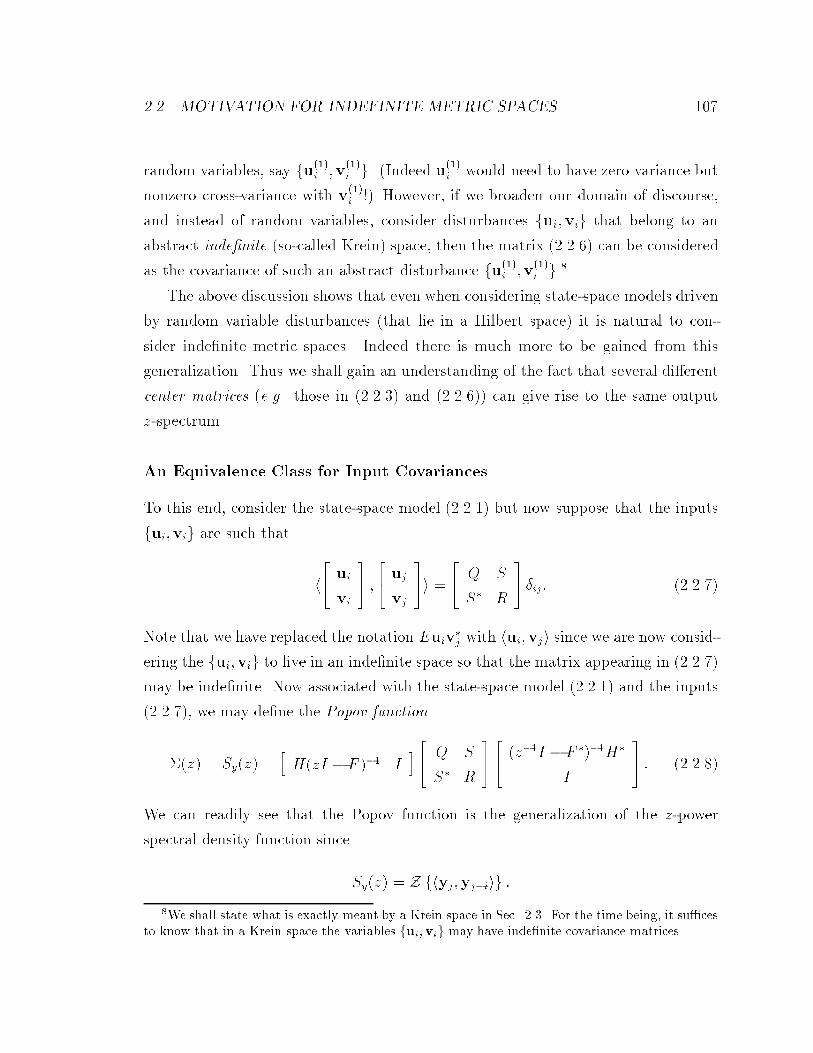
���� MOTIVATION FOR INDEFINITE METRIC SPACES ��
random variables� say fu�i �v�i g� �Indeed u�i would need to have zero variance but
nonzero cross�variance with v�i �� However� if we broaden our domain of discourse�
and instead of random variables� consider disturbances fui�vig that belong to an
abstract inde�nite �so�called Krein� space� then the matrix ������� can be considered
as the covariance of such an abstract disturbance fu�i �v�i g��
The above discussion shows that even when considering state�space models driven
by random variable disturbances �that lie in a Hilbert space� it is natural to con�
sider inde�nite metric spaces� Indeed there is much more to be gained from this
generalization� Thus we shall gain an understanding of the fact that several di�erent
center matrices �e�g� those in ������� and �������� can give rise to the same output
z�spectrum�
An Equivalence Class for Input Covariances
To this end� consider the state�space model ������� but now suppose that the inputs
fui�vig are such that
h�� ui
vi
�� ��� uj
vj
��i �
�� Q S
S� R
�� �ij� ������
Note that we have replaced the notation Euiv�j with hui�vji since we are now consid�
ering the fui�vig to live in an inde�nite space so that the matrix appearing in ������
may be inde�nite� Now associated with the state�space model ������� and the inputs
������� we may de�ne the Popov function
��z� � Sy�z� �hH�zI � F ��� I
i �� Q S
S� R
���� �z��I � F ����H�
I
�� � �������
We can readily see that the Popov function is the generalization of the z�power
spectral density function since
Sy�z� � Z fhyj�yj�iig ��We shall state what is exactly meant by a Krein space in Sec � For the time being� it su�ces
to know that in a Krein space the variables fui�vig may have inde�nite covariance matrices
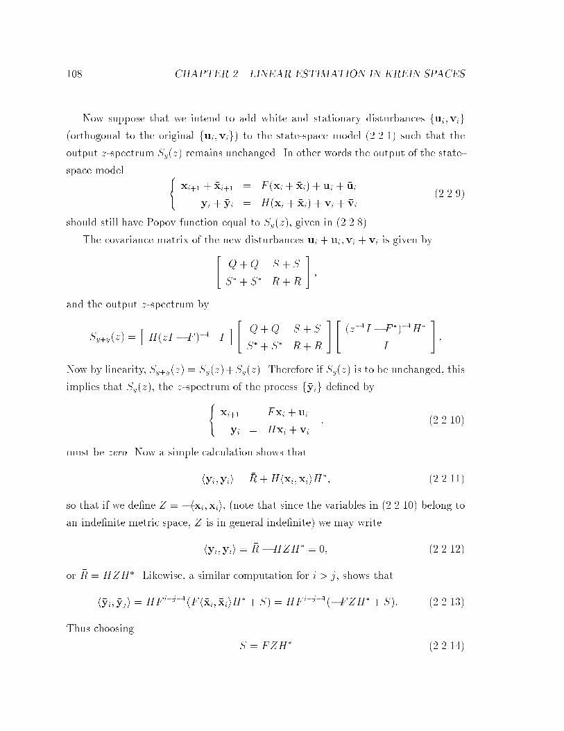
��� CHAPTER �� LINEAR ESTIMATION IN KREIN SPACES
Now suppose that we intend to add white and stationary disturbances f�ui� �vig�orthogonal to the original fui�vig� to the state�space model ������� such that the
output z�spectrum Sy�z� remains unchanged� In other words the output of the state�
space model ���xi�� � �xi�� � F �xi � �xi� � ui � �ui
yi � �yi � H�xi � �xi� � vi � �vi�������
should still have Popov function equal to Sy�z�� given in ��������
The covariance matrix of the new disturbances ui � �ui�vi � �vi is given by�� Q� �Q S � �S
S� � �S� R � �R
�� �
and the output z�spectrum by
Sy��y�z� �hH�zI � F ��� I
i �� Q� �Q S � �S
S� � �S� R� �R
���� �z��I � F ����H�
I
�� �
Now by linearity� Sy��y�z� � Sy�z��S�y�z�� Therefore if Sy�z� is to be unchanged� this
implies that S�y�z�� the z�spectrum of the process f�yig de�ned by
���
�xi�� � F �xi � �ui
�yi � H�xi � �vi� ��������
must be zero� Now a simple calculation shows that
h�yi� �yii � �R �Hh�xi� �xiiH�� ��������
so that if we de�ne Z � �h�xi� �xii� �note that since the variables in �������� belong to
an inde�nite metric space� Z is in general inde�nite� we may write
h�yi� �yii � �R �HZH� � �� ��������
or �R � HZH�� Likewise� a similar computation for i � j� shows that
h�yi� �yji � HF i�j���F h�xi� �xiiH� � �S� � HF i�j����FZH� � �S�� ��������
Thus choosing
�S � FZH� �������
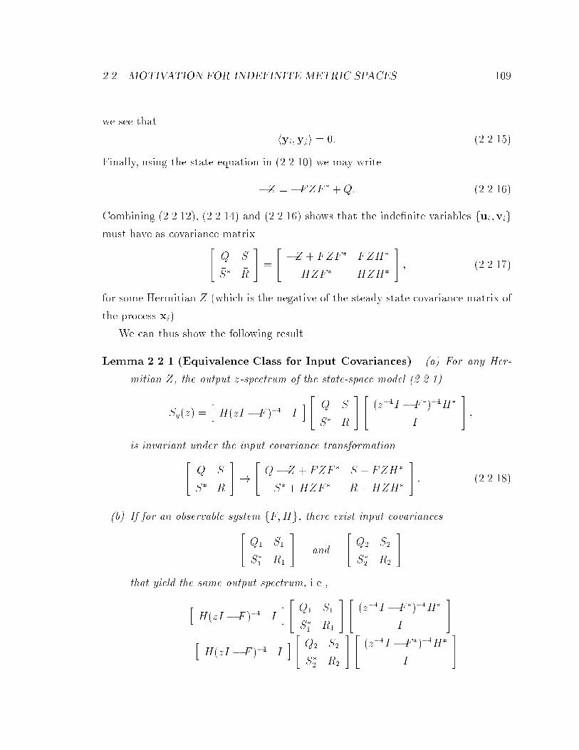
���� MOTIVATION FOR INDEFINITE METRIC SPACES ���
we see that
h�yi� �yji � �� ��������
Finally� using the state equation in �������� we may write
�Z � �FZF � � �Q� ��������
Combining ��������� ������� and �������� shows that the inde�nite variables f�ui� �vigmust have as covariance matrix
�� �Q �S
�S� �R
�� �
�� �Z � FZF � FZH�
HZF � HZH�
�� � �������
for some Hermitian Z �which is the negative of the steady state covariance matrix of
the process �xi��
We can thus show the following result�
Lemma ����� �Equivalence Class for Input Covariances� �a� For any Her�
mitian Z� the output z�spectrum of the state�space model ����
Sy�z� �hH�zI � F ��� I
i�� Q S
S� R
���� �z��I � F ����H�
I
�� �
is invariant under the input covariance transformation�� Q S
S� R
���
�� Q� Z � FZF � S � FZH�
S� �HZF � R �HZH�
�� � ��������
�b� If for an observable system fF�Hg� there exist input covariances�� Q� S�
S�� R�
�� and
�� Q� S�
S�� R�
��
that yield the same output spectrum� i�e��
hH�zI � F ��� I
i �� Q� S�
S�� R�
���� �z��I � F ����H�
I
��
�hH�zI � F ��� I
i �� Q� S�
S�� R�
���� �z��I � F ����H�
I
��

��� CHAPTER �� LINEAR ESTIMATION IN KREIN SPACES
then there exists a unique Hermitian Z such that�� Q� S�
S�� R�
�� �
�� Q� � Z � FZF � S� � FZH�
S�� �HZF � R� �HZH�
�� �
Remark� When fF�Hg is not observable� part �b� of the above Lemma becomes
slightly more complicated �see Chapter �� Although the results presented below
extend to the case where fF�Hg is detectable instead of observable� to simplify the
arguments we shall retain the observability assumption�
Proof of Lemma ������ We have already proven part �a� in the arguments preceding
the statement of the Lemma� Another approach is to directly show via a calculation
that �������� is true for any Hermitian matrix Z � just check that
� �hH�zI � F ��� I
i �� �Z � FZF � FZH�
HZF � HZH�
���� �z��I � F ����H�
I
�� �
is true for any Z � Z��
For part �b�� note that since fQ�� R�� S�g and fQ�� R�� S�g generate the same
output z�spectrum we can write
hH�zI � F ��� I
i �� Q� �Q� S� � S�
S�� � S�� R� �R�
���� �z��I � F ����H�
I
�� � ��
Thus if we de�ne the inde�nite variables f�ui� �vig such that
h�� �ui
�vi
�� ��� �uj
�vj
��i �
�� �Q �S
�S� �R
�� �ij �
�� Q� �Q� S� � S�
S�� � S�� R� �R�
�� �ij�
then the state�space model���
�xi�� � F �xi � �ui
�yi � H�xi � �vi�
must generate zero output z�spectrum� Using the arguments presented before the
statement of the Lemma� this implies that
�Q � �Z � FZF �
�R � HZH�
� � F i�j����FZH� � �S� for i � j

���� MOTIVATION FOR INDEFINITE METRIC SPACES ���
where as before we have de�ned h�xi� �xii � �Z� Note that since F is stable the �rst
of the above equations shows that Z is unique
Moreover� the last equation shows that
O��FZH� � �S� � ��
where
O �hH� F �H� F ��H� � � �
i�
is the observability map� When fF�Hg is observable� O is full rank and we conclude
that
�FZH� � �S � ��
We have thus shown that there exists a unique Hermitian Z such that
�� �Q �S
�S� �R
�� �
�� Q� �Q� S� � S�
S�� � S�� R� �R�
�� �
�� �Z � FZF � FZH�
HZF � HZH�
��
from which the statement of part �b� follows�
Lemma ����� shows the great freedom that is obtained by allowing the disturbances
fui�vig to have an inde�nite covariance matrix� We were thus able to parametrize
all input covariance matrices that gave rise to the same Popov function in terms
of a Hermitian matrix Z� This matrix had the interpretation of being the steady
state covariance of the state vector in a state�space model that generates zero output
spectrum� �The reader at this point may want to verify that the choice Z � ��� where
�� is as in ������� relates the input covariances in ������� and ��������
Another application of the degree of freedom available via the matrix Z� is to
choose Z such that the center matrix in the Popov function drops rank� i�e��
�� Q� Z � FZF � S � FZH�
S� �HZF � R�HZH�
�� �
�� Kp
I
��Re
hK�
p Ii� ��������
In fact� we only require that F have no two eigenvalues such that �i � ���j for the solution to
the Lyapunov equation Z � FZF � � �Q to be unique

��� CHAPTER �� LINEAR ESTIMATION IN KREIN SPACES
This is of signi�cance� since it leads to the following factorization of the Popov function
Sy�z� �hH�zI � F ���Kp � I
iRe
hH�z��I � F ���Kp � I
i�� ��������
In particular� when the transfer matrix H�zI � F ���Kp � I has a stable inverse� the
above factorization is known as the canonical� or spectral� factorization of the Popov
function� As we have seen� the canonical factorization is a key element in H� and
H� estimation and control� We should remark that the above approach can be used
to study solutions of the discrete�time algebraic Riccati equation �DARE� in terms of
factorizations of the Popov function��� Its major bene�t is that it allows one to treat
the positive �semi�de�nite and inde�nite cases in a uni�ed fashion� This approach
will be taken up in Chapter to obtain general existence results for Riccati equations
in the �possibly� inde�nite case�
The results of Lemma ����� are not concerned with the case where the process
fyig is a true stochastic process� i�e�� that its z�spectrum� Sy�z�� is nonnegative on
the unit circle� When that is true� we have a further characterization of the Hermitian
matrices� Z� The result is the KYP Lemma�
Theorem ����� �KYP Lemma� Consider the observable pair fF�Hg� Then the
following two statements are equivalent�
�i� Sy�z� � � for all z � ej� ��F �� where
Sy�z� �hH�zI � F ��� I
i�� Q S
S� R
���� �z��I � F ����H�
I
�� �
�ii� There exists a Hermitian Z such that
�� Q� Z � FZF � S � FZH�
S� �HZF � R �HZH�
�� � �� ��������
�See �McM� � You��� Yak��a for the factorization of rational matrix functions

���� ON KREIN SPACES ���
Remark� The above Theorem has a remarkable interpretation� Note that in view of
Lemma ������ we may write
Sy�z� �hH�zI � F ��� I
i �� Q� Z � FZF � S � FZH�
S� �HZF � R�HZH�
���� �z��I � F ����H�
I
�� �
Thus� Theorem ����� states that Sy�z� is a true z�spectral density function �i�e�� it
is nonnegative de�nite on the unit circle� if� and only if� there exists true stochastic
inputs with nonnegative de�nite covariance�� Q� Z � FZF � S � FZH�
S� �HZF � R �HZH�
�� � ��
that generate it� This has special signi�cance to the problem of stochastic realization
since it states that any nonnegative de�nite rational z�spectral density function can be
realized by a �nite�dimensional state�space model driven by true stochastic processes�
The Theorem also gives a recipe as to how to �nd this realization in terms of the linear
matrix inequality �LMI�� ���������
In the Appendix we shall show how it is possible to use simple Krein space geom�
etry to prove the KYP Lemma� and in fact a slightly more general time�variant
counterpart� For the time being� however� let us proceed with main objective of this
chapter � the development of a theory for linear estimation in Krein spaces�
��� On Krein Spaces
We brie�y introduce the de�nitions and basic properties of Krein spaces� focusing on
those results that we shall need later� Detailed expositions can be found in the books
�Bog� Ist�� IKL�� � Most readers will be familiar with �nite�dimensional �often
called Euclidean� and in�nite�dimensional Hilbert spaces� Finite�dimensional �often
called Minkowski� and in�nite�dimensional Krein spaces share many of the properties
Hilbert spaces� but di�er in some important ways that we shall emphasize in the
following�
De�nition ���� �Krein Spaces� An abstract vector space fK� h�� �ig that satis�es
the following requirements is called a Krein Space�

�� CHAPTER �� LINEAR ESTIMATION IN KREIN SPACES
�i� K is a linear space over C� the complex numbers�
�ii� There exists a bilinear form h�� �i C on K such that
�a� hy�xi � hx�yi�
�b� hax� by� zi � ahx� zi � bhy� zi
for any x�y� z K� a� b C� and where � denotes complex conjugation�
�iii� The vector space K admits a direct orthogonal sum decomposition
K � K� �K�
such that fK�� h�� �ig and fK���h�� �ig are Hilbert spaces� and
hx�yi � �
for any x K� and y K��
Remarks�
�� Recall that Hilbert spaces satisfy not only �i� and �ii���a�� �ii���b� above� but
also the requirement that
hx�xi � � when x � ��
�� The fundamental decomposition of K de�nes two projection operators P� and
P� such that
P�K � K� and P�K � K��Therefore for every x K we can write
x � P�x � P�x � x� � x� � x� K��
Note that for every x K�� we have hx�xi � �� but the converse is not true�
hx�xi � � does not necessarily imply that x K��

���� ON KREIN SPACES ���
�� A vector x K will be said to be positive if hx�xi � �� neutral if hx�xi � ��
or negative if hx�xi � �� Correspondingly� a subspace M� K can be positive�
neutral� or negative� if all its elements are so� respectively�
We now focus on linear subspaces of K� We shall de�ne Lfy�� � � � �yNg as the
linear subspace of K spanned by the elements y��y�� � � � �yN in K� The Gramian of
the collection of elements fy�� � � � �yNg is de�ned as the �N � ��� �N � �� matrix
Ry�� �hyi�yji i�j���N � �������
The re�exivity property� hyi�yji � hyj�yii�� shows that the Gramian is a Hermitian
matrix�
It is useful to introduce some matrix notation here� We shall write the column
vector of the fyig as
y � colfy��y�� � � � �yNg�and denote the above Gramian of the fyig as
Ry�� hy�yi�
� A useful mnemonicdevice for recalling this is to think of the fy�� � � � �yNg as randomvariables! and their Gramian as the covariance matrix!
Ry �hEyiy
�j
i� Eyy��
where E��� denotes expectation!� We use the quotation marks because in our con�
text� the covariance matrix will generally be inde�nite� so we are dealing with some
kind of generalized random variables!� We do not pursue this interpretation here
since our aim is only to provide readers with a convenient device for interpreting the
shorthand notation�
So also if we have two sets of elements fz�� � � � � zMg and fy�� � � � �yNg we shall
write
z � colfz�� z�� � � � � zMg and y � colfy��y�� � � � �yNg�and introduce the �M � ��� �N � �� cross�Gramian matrix
Rzy � �hzi�yji i���Mj���N
�� hz�yi�

��� CHAPTER �� LINEAR ESTIMATION IN KREIN SPACES
Note the property
Rzy � R�yz �
We now proceed with a simple result�
Lemma ���� �Positive and Negative Linear Subspaces� Suppose y�� � � � �yN are
linearly independent elements of K� Then Lfy�� � � � �yNg is a �positive �negative�
subspace of K if� and only if�
Ry � � �Ry � ���
Proof� Since the yi are linearly independent� for any z � � Lfy�� � � � �yNg there
exists a unique k CN�� such that z � k�y� Now
hz� zi � k�hy�yik � k�Ryk�
so that hz� zi � � for all z Lfy�� � � � �yNg� if� and only if� Ry � �� The proof for
Ry � � is similar�
Note that any linear subspace whose Gramian has mixed inertia �both positive and
negative eigenvalues� will have elements in both the positive and negative subspaces�
����� A Geometric Interpretation
Inde�nite metric spaces were perhaps �rst introduced into the solution of physical
problems via the �nite�dimensional Minkowski spaces of special relativity �LEMW���
Ein��� Sch�a � and some geometric insight may be gained by considering the special
��dimensional Minkowski space of Figure ���� de�ned by the inner product
hv��v�i � x�x� � y�y� � t�t��
where
v� � �x�� y�� t��� v� � �x�� y�� t�� and xi� yi� ti C�

���� ON KREIN SPACES ��
t
y
x
Positive subspace
Negative subspace
Neutral cone:
x + y - t = 0 2 2 2
Figure ���� ��dimensional Minkowski space
The �inde�nite� squared norm of each vector v � �x� y� t� is equal to
hv�vi � x� � y� � t��
In this case� we can take K� to be the x� y plane and K� as the t axis� The neutral
subspace is given by the cone� x�� y�� t� � �� with points inside the cone belonging
to the negative subspace� x�� y�� t� � �� and points outside the cone corresponding
to the positive subspace� x� � y� � t� � ��
Moreover� any plane passing through the origin but lying outside the neutral
cone will have positive de�nite Gramian� and any line passing through the origin
and inside the neutral cone will have negative de�nite Gramian� So also� any plane
passing through the origin that intersects the neutral cone will have Gramian with
mixed inertia� and any plane tangent to the cone will have singular Gramian�
Two key di�erences between Krein spaces and Hilbert spaces are the existence
of neutral and isotropic vectors� As mentioned earlier� a neutral vector is a nonzero
vector that has zero length� an isotropic vector is a nonzero vector lying in a linear
subspace of K that is orthogonal to every element in that linear subspace� There
are obviously no such vectors in Euclidean or Hilbert spaces� In the Minkowski
space described above�h� �
p�iis a neutral vector� and if one considers the
��� CHAPTER �� LINEAR ESTIMATION IN KREIN SPACES
linear subspace Lnh
� �p�i�h p
� � �io
thenh� �
p�iis also an isotropic
vector in this linear subspace���
��� Projections in Krein Spaces
An important notion in both Hilbert and Krein spaces is that of the projection onto
a subspace�
De�nition ���� �Projections in Krein Space� Given the element z in K� andthe elements fy��y�� � � � �yNg also in K� we de�ne "z to be the projection of z onto
Lfy��y�� � � � �yNg if�
z � "z� #z ������
where "z Lfy�� ����yNg and #z satis�es the orthogonality condition
#z Lfy�� ����yNg�
or equivalently� h#z�yii � � for i � �� �� � � � � N �
In Hilbert space projections always exist and are unique� However� in Krein space
this is not always the case� Indeed we have the following result� where for simplicity
we have written Lfyg �� Lfy�� � � � �yNg�
Lemma ���� �Existence and Uniqueness of Projections� In the Hilbert space
setting� projections always exist and are unique� However� in the Krein space setting�
�a� If the Gramian matrix Ry � hy�yi is nonsingular� then the projection of z onto
Lfyg exists� is unique� and is given by
"z � hz�yihy�yi��y � RzyR��y y� ������
�b� If the Gramian matrix Ry � hy�yi is singular� then��We should note that Minkowski �and Krein� spaces are closely related to the hyperbolic spaces
�rst introduced by NI Lobachevskii in ���� �see �Lob��� in his researches on non�Euclideangeometry In what follows we shall make use of only some rudimentary facts from hyperbolicgeometry For more on this subject consult �Fen�� and �Ive�

���� PROJECTIONS IN KREIN SPACES ���
�i� If R�Ryz� � R�Ry� �where R�A� denotes the column range space of the
matrix A�� the projection "z exists but is nonunique� In fact� "z � k�oy�
where ko is �any solution to the linear matrix equation
Ryko � Ryz � ������
�ii� If R�Ryz� � R�Ry�� the projection "z does not exist�
Proof� Suppose "z is a projection of z onto the desired space� By ������� we can
write
z � k�oy � #z�
for some ko CN��� Since h#z�yi � ��
Rzy � hz�yi � k�ohy�yi� � � k�oRy� �����
If Ry is nonsingular then the solution for k in ����� is unique and the projection is
given by ������� If Ry is singular� two things may happen� eitherR�Ryz� � R�Ry� in
which case ����� will have a nonunique solution �since any k�� in the left null space
of Ry can be added to k�o�� or R�Ryz� � R�Ry� in which case the projection does not
exist since a solution to ����� does not exist�
In Hilbert spaces the projection always exists because it is always true that
R�Ryz� � R�Ry�� or equivalently� that N �Ry� � N �Rzy�� where N �A� is the right
nullspace of the matrix A� To show this� suppose that l N �Ry�� Then
Ryl � � � l�Ryl � �
� l�hy�yil � hl�y� l�yi � �
� l�y � ��
where the last equality follows from the fact that in Hilbert spaces hx�xi � � �x � �� We now readily conclude that hz� l�yi � Rzy l � �� i�e� � l N �Rzy� and hence
N �Ry� � N �Rzy�� Therefore a solution to ����� �and hence a projection� always
exists in Hilbert spaces�
��� CHAPTER �� LINEAR ESTIMATION IN KREIN SPACES
In Hilbert spaces the projection is also unique because if k� and k� are two di�erent
solutions to ������ then �k� � k���Ry � �� But the above argument shows that we
must then have �k� � k��y � �� Hence the projection
"z � k��y � k��y
is unique�
The proof of the above lemma shows that in Hilbert spaces the singularity of Ry
implies that the fyig are linearly dependent� i�e� �
det�Ry� � � � k�y � � for some vector k CN���
In the Krein space setting� all we can deduce from the singularity of Ry is that
there exists a linear combination of the fyig that is orthogonal to every vector in
Lfy�� ����yNg� i�e� � that Lfy�� ����yNg contains an isotropic vector� This follows by
noting that for any complex matrix k�� and for any k in the null space of Ry� we have
k��Ryk � hk��y� k�yi � � �
which shows that the linear combination k�y is orthogonal to k��y� for every k�� i�e� �
k�y is an isotropic vector in Lfyg�Standing Assumption� Since existence and uniqueness will be important for all
our future results� we shall make the standing assumption that the Gramian
Ry is nonsingular�
����� Vector�Valued Projections
Consider the n�vector z � colfz�� � � � � zng composed of elements zi K� and the set
fy�� � � � �yNg where yj K� project each element zi onto Lfy�� � � � �yNg to obtain "zi�
We de�ne "z � colf"z�� � � � � "zng as the projection of z onto Lfy�� � � � �yNg� �Strictly
speaking� we should call "z Kn the projection of z Kn onto Lnfy�� � � � �yNg� sinceit is an element of Lnfy�� � � � �yNg� and not Lfy�� � � � �yNg� However� for simplicity�
we shall generally use the looser terminology�

���� PROJECTIONS IN KREIN SPACES ���
It is easy to see that the results on the existence and uniqueness of projections in
Lemma ���� continue to hold in the vector case as well�
In this connection� it will be useful to introduce a slight generalization of the
de�nition of Krein spaces that was given in Sec� ���� There� in De�nition ������ we
mentioned that K should be linear over the �eld of complex numbers� C� However� it
turns out that we can replace C with any ring S� In other words� the �rst two axioms
for Krein spaces can be replaced by
�i� K is a linear space over the ring S�
�ii� There exists a bilinear form h�� �i S on K such that
�a� hy�xi � hx�yi�
�b� hax� by� zi � ahx� zi � bhy� zi
for any x�y� z K and a� b S� and where the operation � depends on the ring
S�
When the inner product h�� �i S is positive� fK� h�� �ig is referred to as a module�
Thus the third axiom for Krein spaces can be replaced by
�iii� The vector space K admits a direct orthogonal sum decomposition
K � K� �K�
such that fK�� h�� �ig and fK���h�� �ig are modules� and hx�yi � � for any
x K� and y K��
The most important case for us is when S is a ring of complex matrices� and the
operation � denotes Hermitian transpose�
The point of this generalization is that we can now directly de�ne the projection
of a vector z Kn onto Lnfy�� � � � �yNg as an element "z Lnfy�� � � � �yNg� such that
"z � k�oy � k�o Cn�N
where k is such that
� � hz� k�oy�yi �� Rzy � k�oRy

��� CHAPTER �� LINEAR ESTIMATION IN KREIN SPACES
or
k�oRy � Rzy�
Finally� let us remark that to avoid additional notational burden� we shall often
refrain from writing Kn and shall simply use the notation K for any Krein space� The
ring S over which the Krein space is de�ned will be obvious from the context�
��� Projections and Quadratic Forms
In Hilbert space� projections extremize �minimize� certain quadratic forms� as we shall
brie�y �rst describe� In Krein spaces� we can in general only assert that projections
stationarize such quadratic forms� further conditions need to be met for the stationary
points to be extrema �minima�� This will be elaborated in Sec� ������ in the context of
�what we shall call� a stochastic minimization problem� In Sec� ������ we shall study
a closely related quadratic form arising in what we shall call a partially equivalent
deterministic minimization problem�
����� Stochastic Minimization Problems in Hilbert and Krein
Spaces
Consider a collection of elements fy�� � � � �yNg in a Krein space K with inde�nite
inner product h�� �i� Let z � colfz�� � � � � zMg be some column vector of elements
in K� and consider an arbitrary linear combination of fy�� � � � �yNg� say k�y� where
k� CM���N�� and y � colfy�� � � � �yNg� A natural object to study is the error
Gramian
P �k� � hz � k�y� z� k�yi� �������
To motivate the subsequent discussion� let us �rst assume that the fyig and fzjgbelong to a Hilbert space of zero�mean random variables� and that their variance
and cross�variances are known� In this case the inner product is hzi�yjiH � Eziy�j
�where E��� denotes expectation�� and P �k� is simply the mean�square�error �or error

���� PROJECTIONS AND QUADRATIC FORMS ���
variance� matrix in estimating z using k�y� viz��
P �k� � E�z� k�y��z� k�y�� � kz� k�yk�H� say�
It is well�known that the linear least�mean�square estimate� which minimizesP �k��
is given by the projection of z on Lfyg�
"z � k�oy�
where
k�o � Ezy� �Eyy� �� � RzyR��y �
The simple proof will be instructive� Thus note that
P �k� � kz� k�yk�H � kz� "z� "z� k�yk�H � kz� "zk�H � k"z� k�yk�H�
since by the de�nition of "z� it holds that
hz� "z� "z� k�yiH � ��
Clearly� since "z � k�oy�
P �k� � P �ko��
with equality achieved only when k � ko�
However� this argument breaks down when the elements are in a Krein space�
since then we could have
k"z� k�yk� � kk�oy� k�yk� � �� even if ko � k�
All we can assert is that
k�oy� k�y � an isotropic vector in the linear subspace spanned by fy�� � � � �yNg�
Moreover� since kk�oy � k�yk� could be negative� it is not true that P �k� will be
minimized by choosing k � ko� So a closer study is necessary�
We shall start with a de�nition�

�� CHAPTER �� LINEAR ESTIMATION IN KREIN SPACES
De�nition ����� �Stationary Point� The matrix ko CN���M�� is said to be
a stationary point of an �M � �� � �M � �� matrix quadratic form in k� say
P �k� � A�Bk � k�B� � k�Ck�
if� and only if� koa is a stationary point of the �scalar quadratic form a�P �k�a for
all complex column vectors a CM��� i�e� � if� and only if�
�a�P �k�a
�ka
k�ko
� ��
Now we can prove the following�
Lemma ����� �Condition for Minimum� A stationary point of P �k� is a mini�
mum if� and only if� for all a CM��
��a�P �k�a
��ka��
k�ko
� �� �������
Moreover� it is a unique minimum if� and only if�
��a�P �k�a
��ka��
k�ko
� �� �������
Proof� Writing the Taylor series expansion of a�P �k�a around the stationary point
ko yields �since a�P �k�a is quadratic in ka�
a�P �k�a � a�P �ko�a��a�P �k�a
�ka
k�ko �z �
��
��k�ko�a�a��k�ko�� ��a�P �k�a
��ka��
k�ko
��k�ko�a�
or equivalently�
a�P �k�a� a�P �ko�a � a��k � ko�� �
�a�P �k�a
��ka��
k�ko
� �k � ko�a�
Using the above expression� we see that ko is a minimum� i�e� � a�P �k�a�a�P �ko�a � �
for all k � ko if� and only if� ������� is satis�ed� Moreover� ko will be a unique

���� PROJECTIONS AND QUADRATIC FORMS ���
minimum� i�e� � a�P �k�a � a�P �ko�a � � for all k � ko if� and only if� ������� is
satis�ed�
Let us now return to the error Gramian P �k� in �������� and expand it as
P �k� � hz� ziK � hz�yiKk � k�hy� ziK � k�hy�yiKk� ������
or more compactly�
P �k� �hI �k�
i �� Rz Rzy
Ryz Ry
���� I
�k
�� � �������
Note that the center matrix appearing in ������� is the Gramian of the vector colfz�yg�
������������
�����
��
���
����������������
�
�
Lfyg
zz� "z
"z � k�oy
Figure ���� The projection "z � k�oy stationarizes the error Gramian P �k� � hz �k�y� z� k�yi over all k�y Lfyg�
For this particular quadratic form� we can use the easily veri�ed triangular fac�
torization �recall our standing assumption that Ry is nonsingular���� Rz Rzy
Ryz Ry
�� �
�� I RzyR
��y
� I
���� Rz �RzyR
��y Ryz �
� Ry
���� I �
R��y Ryz I
�� �������

��� CHAPTER �� LINEAR ESTIMATION IN KREIN SPACES
to write
a�P �k�a �
ha� a�k� � a�RzyR
��y
i�� Rz �RzyR��y Ryz �
� Ry
���� a
ka�R��y Ryza
�� �������
Calculating the stationary point of P �k�� and the corresponding condition for a
minimum� is now straightforward� Note� moreover� that Ry nonsingular implies that
the stationary point is unique�
Theorem ����� �Stationary Point of the Error Gramian� When Ry is nonsin�
gular� ko� the unique coe�cient matrix in the projection of z onto Lfyg�
"z � k�oy � ko � R��y Ryz
yields the unique stationary point of the error Gramian
P �k��� hz � k�y� z� k�yi �
hI �k�
i �� Rz Rzy
Ryz Ry
���� I
�k
�� �������
over all k CN���M��� Moreover� the value of P �k� at the stationary point is
given by
P �ko� � Rz �RzyR��y Ryz�
Proof� The claims follow easily from ������ by di�erentiation�
Further di�erentiation and use of Lemma ����� yields the following result�
Corollary ����� �Condition for a Minimum� In Theorem ���� ko is a unique
minimum if� and only if�
Ry � ��
i�e�� Ry is not only nonsingular but also positive de�nite�

���� PROJECTIONS AND QUADRATIC FORMS ��
����� A Partially Equivalent Deterministic Problem
We shall now consider what we call a partially equivalent deterministic problem� We
refer to it as deterministic� because it involves computing the stationary point of a
certain scalar quadratic form over ordinary complex variables �not Krein space ones��
Moreover� it is called partially equivalent since its solution� i�e� � the stationary point�
is given by the same expression as the projection of one suitably de�ned Krein space
vector onto another� while the condition for a minimum is di�erent than that for the
Krein space projection�
To this end� consider the scalar second order form
J�z� y���hz� y�
i �� Rz Rzy
Ryz Ry
���� �� z
y
�� �������
where the central matrix is the inverse of the Gramian matrix in the stochastic prob�
lem of Theorem ����� � see �������� Suppose we seek the stationarizing element zo for
a given y� �Of course now we assume not only that Ry is nonsingular� but so also
the block matrix appearing in �������� Note that z and y are no longer bold face�
meaning that they are to be regarded as �ordinary� vectors of complex numbers�
Referring to the discussion at the beginning of Sec� ����� on Hilbert spaces� the
motivation for this problem is the fact that for jointly Gaussian random vectors
fz�yg� the linear least�mean�squares estimate can be found as the conditional mean
of the conditional density pzy�z� y�py�y�� When fz�yg are zero�mean with covari�
ance matrix
�� Rz Rzy
Ryz Ry
��� taking logarithms of the conditional density results in the
quadratic form �������� which is the negative of the so�called log�likelihood function�
In this case� the relation between ������� and the projection follows from the fact
that the linear least�mean�squares estimate is the same as the maximum likelihood
estimate �obtained by minimizing ��������� With this motivation� we now introduce
and study the quadratic form J�z� y�� without any reference to fz�yg being Gaussian�
Theorem ����� �Deterministic Stationary Point� Suppose both Ry and the block
matrix in ������ are nonsingular� Then

��� CHAPTER �� LINEAR ESTIMATION IN KREIN SPACES
�a� The stationary point zo of J�z� y� over z is given by
zo � RzyR��y y�
�b� The value of J�z� y� at the stationary point is
J�zo� y� � y�R��y y�
Corollary ����� �Condition for a Minimum� In Theorem ���� zo is a mini�
mum if� and only if�
Rz �RzyR��y Ryz � ��
Proof� We note that �see ��������
�� Rz Rzy
Ryz Ry
����
�
�� I �
�R��y Ryz I
���� Rz �RzyR
��y Ryz �
� Ry
���� �� I �RzyR
��y
� I
��
so that we can write
J�z� y� �
h�z� � y�R��y Ryz� y�
i�� Rz �RzyR��y Ryz �
� Ry
���� �� �z �RzyR
��y y�
y
�� �
It now follows by di�erentiation that the stationary point of J�z� y� is equal to zo �
RzyR��y y� and that J�zo� y� � y�R��y y� To prove the Corollary� we di�erentiate once
again� and use Lemma ������
Remark �� Comparing the results of Theorems ����� and ����� shows that the
stationary point zo� of the scalar quadratic form �������� is given by a formula that is
exactly the same as that in Theorem ����� for the Krein space projection of a vector z

���� PROJECTIONS AND QUADRATIC FORMS ���
onto the linear span Lfyg� However� in Theorem ����� there is no Krein space� z and
y are just vectors �in general of di�erent dimensions� in Euclidean space and zo is not
the projection of z onto the vector y� What we have shown in Theorem ����� is that
by properly de�ning the scalar quadratic form as in ������� using coe�cient matrices
Rz� Ry� Rzy� and Ryz that are arbitrary� but can be regarded as being obtained from
Gramians and cross Gramians of some Krein space vectors fz�yg� we can calculate
the stationary point using the same recipe as in Theorem ������
Remark �� However� although the stationary points of the matrix quadratic form
P �k� and the scalar quadratic form J�z� y� are found by the same computations� the
two forms do not necessarily simultaneously have a minimum� since one requires the
condition Ry � � �Cor� ������� and the other requires the condition Rz�RzyR��y Ryz �
� �Cor� ������� This is the major di�erence from the classical Hilbert space context
where we have
h�� z
y
�� ��� z
y
��iH �
�� Rz Rzy
Ryz Ry
�� � �� ��������
When �������� holds� the approaches of Theorems ����� and ����� give equivalent
results�
Corollary ���� �Simultaneous Minima� For vectors z and y of linear indepen�
dent elements in a Hilbert space H� the conditions Rz �RzyR��y Ryz � � and Ry � �
occur simultaneously�
Proof� Immediate from the factorization ��������
We shall see in more detail in Chapters � and � and to some extent in Sec� �����
that this di�erence is what makesH� �and risk�sensitive and �nite memory adaptive
�ltering� results di�erent from H� results� Brie�y� H� problems will lead directly
to certain inde�nite quadratic forms� to stationarize them we shall �nd it useful to
set up the corresponding Krein space problem and appeal to Theorem ������ While
this will give an algorithm� further work will be necessary to check for the minimum
condition of Theorem ����� in the H� problem�

��� CHAPTER �� LINEAR ESTIMATION IN KREIN SPACES
It is this di�erence that leads us to say that the deterministic problem is only
partially equivalent to the stochastic problem of Sec� ������ �We may remark that we
are making a distinction between equivalence and duality!� one can in fact de�ne
duals to both the above problems� but we defer this topic to Chapter ��
Remark � Finally� recall that Lemma ���� on the existence and uniqueness of
the projection implies that the stochastic problem of Theorem ����� has a unique
solution if� and only if� Ry is nonsingular� thus explaining our standing assumption�
The following result is the analog for the deterministic problem�
Lemma ����� �Existence of Stationarizing Solutions� The deterministic prob�
lem of Theorem ��� has a unique stationarizing solution for all y if� and only if� Ry
is nonsingular�
Proof� Let us denote �� Rz Rzy
Ryz Ry
����
�
�� A B
B C
�� �
so that
J�z� y� �hz� y�
i �� A B
B� C
���� z
y
�� �
If J�z� y� has a unique stationarizing solution for all y then A must be nonsingular
�since by di�erentiation the stationary point must satisfy the equation Azo � By��
But the invertibility of A and the whole center matrix appearing in J�z� y� imply the
invertibility of the Schur complement C �B�A��B� But it is easy to check that this
Schur complement must be the inverse of Ry� Thus Ry must be invertible�
On the other hand if Ry is invertible then the deterministic problem has a unique
stationarizing solution as given by Theorem ������
����� Alternative Inertia Conditions for Minima
In many cases it can be complicated to directly check for the positivity condition of
the deterministic problem� namelyRz�RzyR��y Ryz � �� On the other hand� it is often

���� PROJECTIONS AND QUADRATIC FORMS ���
easier to compute the inertia �the number of positive� negative and zero eigenvalues�
of Ry itself� This often su�ces �SHK��b� SHK��a� SHK�� �
Lemma ���� �Inertia Conditions for Deterministic Minimization� �a� If Ry
and Rz are nonsingular� then the deterministic problem of Theorem ��� will
have a minimizing solution �i�e� Rz �RzyR��y Ryz will be � �� if� and only if�
I��Ry � I��Rz � I���Ry �RyzR��z Rzy� � ��������
where I��A denotes the negative inertia �number of negative eigenvalues� of A�
�b� When Rz � � �rather than just being nonsingular� then we will have a minimiz�
ing solution if� and only if�
I��Ry � I��Ry �RyzR��z Rzy � ��������
i�e� if� and only if� Ry and Ry �RyzR��z Rzy have the same inertia�
Proof� If Ry and Rz are both nonsingular� then equating the lower�upper and upper�
lower block triangular factorizations of the Gramian matrix in ������� will yield the
result that�� Rz �RzyR
��y Ryz �
� Ry
�� and
�� Rz �
� RyRyzR��z Rzy
��
are congruent� By Sylvester$s Law that congruent matrices have the same inertia
�GL�� � we have
I��Rz �RzyR��y Ryz � I��Ry � I��Rz � I���Ry �RyzR
��z Rzy� �
Now if �������� holds� then I��Rz �RzyR��y Ryz � �� so that Rz �RzyR
��y Ryz � ��
Conversely if I��Rz �RzyR��y Ryz � �� then �������� holds�
When Rz � �� we have I��Rz � �� and �������� follows immediately�
The general results presented so far can be made even more explicit when there
is more structure in the problems� In particular� we shall see that when we have

��� CHAPTER �� LINEAR ESTIMATION IN KREIN SPACES
state�space structure both Rz and Ry � RyzR��z Rzy are block�diagonal� Moreover�
a Krein space Kalman �lter! will yield a direct method for computing the inertia
of Ry� Thus� when we have state�space structure� it will be much easier to use the
results of Lemma ����� than to directly check for the positivity of Rz � RzyR��y Ryz
�HSK�c� SHK��b� SHK��a� SHK�� �
��� StateSpace Structure
One approach at this point is to begin by assuming that the components fyjg of y
arise from an underlying Krein space state�space model� However� to better moti�
vate the introduction of such state�space models� we shall start with the following
�inde�nite� quadratic minimization problem�
Consider a system described by the state�space equations
���xj�� � Fjxj �Gjuj� � � j � N
yj � Hjxj � vj�������
where Fj Cn�n� Gj Cn�m and Hj Cp�n are given matrices and the initial state
x� Cn� the driving disturbance uj Cm� and the measurement disturbance vj Cp�are unknown complex vectors� The output yj Cp is assumed known for all j�
In many applications one is confronted with the following deterministic minimiza�
tion problem� Given fyjgNj��� minimize over x� and fujgNj�� the quadratic form
J�x�� u� y� � x������ x� �
XN
j��
hu�j v�j
i �� Qj Sj
S�j Rj
���� �� uj
vj
�� � �������
subject to the state�space constraints �������� and where Qj Cm�m� Sj Cm�p�Rj Cp�p� �� Cn�n are �possibly inde�nite� given Hermitian matrices�
The above deterministic quadratic form is usually encountered in �ltering prob�
lems� a special case that we shall see in the nect chapter is the H� �ltering problem
where the weighting matrices are ��� Qj � I and Rj �
�� I �
� ��fI
��� and where Hi
is now replaced by colfHi� Lig� Another application arises in adaptive �ltering� in

���� STATE�SPACE STRUCTURE ���
which case we usually have uj � � and Fj � I �SK�b� HSK��a � In the general
case� however� �� represents the penalty on the initial state� and fQj� Rj � Sjg repre�
sents the penalty on the driving and measurement disturbances fuj� vjg� �There is
also a dual! quadratic form that arises in control applications� which we shall study
elsewhere��
Such deterministic problems can be solved via a variety of methods� such as dy�
namic programming or Lagrange multipliers �see e�g� � �BB�� �� but we shall �nd it
easier to use the equivalence discussed in Sec� ���� construct a �partially� equivalent
Krein space �or stochastic� problem� In order to do so we �rst need to express the
J�x�� u� y� of ������� in the form of ������� of Sec� ������
For this� we �rst introduce some vector notation� Note that the states fxjg and the
outputs fyjg are linear combinations of the fundamental quantities fx�� fuj� vjgNj��g�We introduce �the state transition matrix�
%�j� k� � Fj�� � � � Fk��� j � k � %�j� j� � I�
and de�ne
hjk�� HjFj�� � � � Fk��Gk � Hj%�j� k�Gk
as the response at time j to an impulse at time k � j �assuming both x� � � and
vk � ���
Then with
y�� colfy�� � � � � yNg � u
�� colfu�� � � � � uNg � v
�� colfv�� � � � � vNg
the state�space equations ������� allow us to write
y � Ox� � &u � v �hO &
i �� x�
u
��� v �������
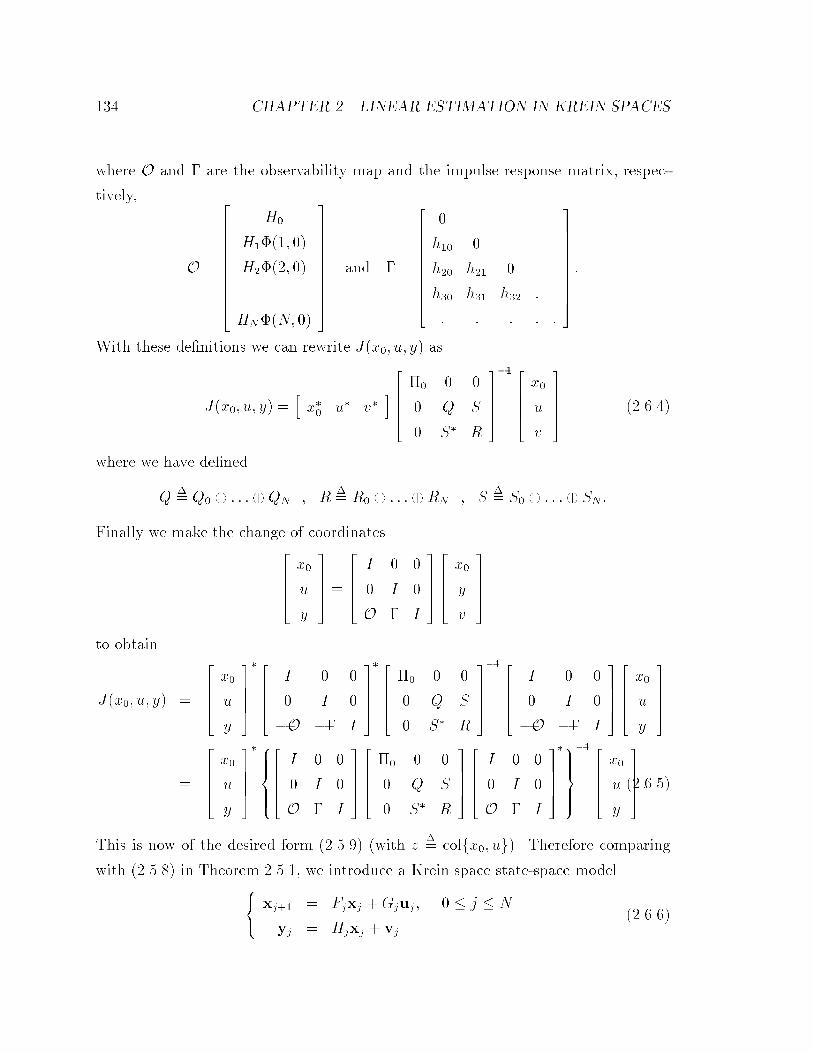
�� CHAPTER �� LINEAR ESTIMATION IN KREIN SPACES
where O and & are the observability map and the impulse response matrix� respec�
tively�
O �
� �
H�
H�%��� ��
H�%��� �����
HN%�N� ��
������������
and & �
� �
�
h�� �
h�� h�� �
h�� h�� h�� �
� � � � �
������������
With these de�nitions we can rewrite J�x�� u� y� as
J�x�� u� y� �hx�� u� v�
i� ��� � �
� Q S
� S� R
�����
�� � �x�
u
v
����� ������
where we have de�ned
Q�� Q� � � � ��QN � R
�� R� � � � ��RN � S
�� S� � � � �� SN �
Finally we make the change of coordinates� �x�
u
y
����� �
� �I � �
� I �
O & I
�����
� �x�
y
v
�����
to obtain
J�x�� u� y� �
� �x�
u
y
�����
� � �
I � �
� I �
�O �& I
�����
� � �
�� � �
� Q S
� S� R
�����
�� � �
I � �
� I �
�O �& I
�����
� �x�
u
y
�����
�
� �x�
u
y
�����
����������
� �I � �
� I �
O & I
�����
� ��� � �
� Q S
� S� R
�����
� �I � �
� I �
O & I
�����
����������
�� � �x�
u
y
����� ��������
This is now of the desired form ������� �with z�� colfx�� ug�� Therefore comparing
with ������� in Theorem ������ we introduce a Krein space state�space model���xj�� � Fjxj �Gjuj � � � j � N
yj � Hjxj � vj�������

���� STATE�SPACE STRUCTURE ���
where the initial state� x�� and the driving and measurement disturbances� fujg and
fvjg are such that
h
� �uj
vj
x�
����� �
� �uk
vk
x�
�����i �
� �
�� Qj Sj
S�j Rj
�� �jk �
� ��
����� � ������
The condition ������ is the Krein space version of the usual assumption made in
the stochastic �Hilbert space� state�space models� viz�� that the initial condition x�
and the driving and measurement disturbances fui�vig are zero�mean uncorrelated
random variables with variance matrices �� and
�� Qj Sj
S�j Rj
��� respectively� and that
the fui�vig form a white �uncorrelated� sequence� As mentioned before� the Krein
space elements can be thought of as some kind of generalized random variables�
Now if� as was done earlier� we de�ne
y � colfy�� � � �yNg � u � colfu�� � � �uNg � v � colfv�� � � �vNg
then we can use the state�space model ������� to write� �x�
u
y
����� �
� �I � �
� I �
O & I
�����
� �x�
u
v
����� �������
and to see that
h
� �x�
u
y
����� �
� �x�
u
y
�����i �
� �I � �
� I �
O & I
�����
� �
�� � �
� Q S
� S� R
�����
� �I � �
� I �
O & I
�����
�
� �������
which is exactly the inverse of the central matrix appearing in expression ������� for
J�x�� u� v�� Therefore� referring to Theorems ����� and ������ the main point is that
to �nd the stationary point of J�x�� u� y� over fx�� ug� we can alternatively �nd the
projection of fx��ug onto Lfyg in the Krein space model ��������
Now that we have identi�ed the stochastic and deterministic problems when a
state�space structure is assumed� we can give the analogs of Theorems ����� and
������

��� CHAPTER �� LINEAR ESTIMATION IN KREIN SPACES
Lemma ����� �Stochastic Interpretation� Suppose z � colfx��ug and y are re�
lated through the state�space model ������������ and that Ry given by ����� is
nonsingular� Then the stationary point of the error Gramian
hz� k�y� z� k�yi ��������
over all k�y is given by the projection�� "x�jN
"ujN
�� �
�� ��O�Q&� � S
��R��y y ��������
where
Ry � O��O� �h& I
i �� Q S
S� R
���� &�
I
�� � ��������
Moreover this stationary point is a minimum if� and only if� Ry � ��
We can now also give the analog result to Theorem ������
Lemma ����� �Deterministic Quadratic Form� The expression�� "x�jN
"ujN
�� �
�� ��O�Q&� � S
��R��y y ��������
yields the stationary point of the quadratic order form�
J�x�� u� y� � x������ x� �
XN
j��
hu�j �yj �Hjxj��
i �� Qj Sj
S�j Rj
���� �� uj
yj �Hjxj
�� �
�������
over x� and u � colfu�� � � � � uNg� and subject to the state�space constraints���xj�� � Fjxj �Gjuj� � � j � N
yj � Hjxj � vj
In particular� when Sj � �� the quadratic form is
J�x�� u� y� � x������ x��
XN
j��u�jQ
��j uj �
XN
j���yj �Hjxj�
�R��j �yj �Hjxj�� ��������
The value of J�x�� u� y� �with either Sj � � or Sj � �� at the stationary point is
J�"x�jN � "ujN � y� � y�R��y y�
���� STATE�SPACE STRUCTURE ��
����� The Conditions for a Minimum
As mentioned earlier� the important point is that the conditions for minima in these
two problems are di�erent� Ry � � in the stochastic problem� and
M�� Rz �RzyR
��y Ryz � � where z � colfx��ug
in the deterministic problem� In the state�space case Ry is given by ��������� In
this section we shall explore the condition for a deterministic minimum under the
state�space assumption� First note that for M we have
M �
�� �� �
� Q
���
�� �� �
� Q
���� O�&� �Q��S
��R��y
hO & � S�Q��
i �� �� �
� Q
�� �
�� �� ���O�R��y O�� ���O�R��y �&Q� S��
��Q&� � S�R��y O�� Q� �Q&� � S�R��y �&Q� S��
�� � ��������
Now we know thatM � � if� and only if� both the ��� �� block entry in �������� and
its Schur complement are positive de�nite� The ��� �� block entry may be identi�ed
as the Gramian of the error x� � "x�jN � i�e��
�� ���O�R��y O�� � hx� � x�jN�x� � x�jNi �� P�jN � �������
To obtain a nice form for the Schur complement of the ��� �� block entry� say '�
we have to use a little matrix algebra� Recall that
Ry � O��O� �h& I
i �� Q S
S� R
���� &�
I
��
�hO & � S�Q��
i �� �� �
� Q
���� O�
&� �Q��S
���R � S�Q��S�
Using the second expression for Ry� and a well�known matrix inversion formula� leads
to the expression
M�� �
�� ���� �
� Q��
���
�� O�
&� �Q��S
�� �R � S�Q��S���
hO & � S�Q��
i�
��������

��� CHAPTER �� LINEAR ESTIMATION IN KREIN SPACES
Now we use another well known fact� the ����� block element of M�� is just '��
�where '�� exists sinceM is positive�de�nite�� Therefore the condition now becomes
Q�� � �&� �Q��S��R� S�Q��S����& � S�Q��� � ��
so that we have the following result�
Lemma ���� �A Condition for a Minimum� If Q and R� S�Q��S are invert�
ible� a necessary and su�cient condition for the stationary point of Lemma ��� to
be a minimum is that
�i� P�jN � �� and
�ii� Q�� � �&� �Q��S��R� S�Q��S����& � S�Q��� � ��
When S � �� the second condition becomes Q�� � &�R��& � ��
The conditions of Lemma ����� need to be reduced further in order to provide
useful computational tests� This can be done in several ways� leading to more speci�c
tests� One interesting way is by showing that Q����&��Q��S��R�S�Q��S����&�
S�Q��� may be regarded as the Gramian matrix of the output of a so�called backwards
dual state�space model� This identi�cation will be useful in studying the H� control
problem �and in other ways�� but we shall not pursue it here�
Instead we shall use the alternative inertia conditions of Lemma ����� to circum�
vent the need for direct analysis of the matrix Rz �RzyR��y Ryz � Recall from Lemma
����� that if Rz � �� a unique minimizing solution to the deterministic problem of
Theorem ����� exists if� and only if Ry and Ry � RyzR��z Rzy have the same inertia�
However� for the state�space structure that we are considering�
Rz �
�� �� �
� Q
��
so that after some simple algebra we have
Ry�RyzR��z Rzy � R�S�Q��S � �R��S��Q��� S���� � ���RN�S�NQ��N SN �� ��������
Thus Ry �RyzR��z Rzy is block�diagonal� and we have the following result�

��� RECURSIVE FORMULAS ���
Lemma ���� �Inertia Condition for Minimum� If �� � � and Q � �� then a
necessary and su�cient condition for the stationary point of Lemma ��� to be a
minimum is that the matrices Ry and R � S�Q��S have the same inertia�
In particular� if S � �� then Ry and R must have the same inertia�
As we shall see in the next section� the Krein space Kalman �lter provides the
block triangular factorization of Ry� and thereby allows one to easily compare the
inertia of Ry and R � S�Q��S�
�� Recursive Formulas
So far we have obtained global expressions for computing projections and for checking
the conditions for deterministic and stochastic minimization� Computing the projec�
tion requires inverting the Gramian matrix Ry� and checking for the minimization
conditions requires checking the inertia of Ry� both of which require O�N�� �where
N is the dimension of Ry� computations�
The key consequence of state�space structure in Hilbert space is that the compu�
tational burden of �nding projections can be signi�cantly reduced� to O�Nn�� �where
n is the dimension of the state�space model�� by using the Kalman �lter recursions�
Moreover� the Kalman �lter also recursively factors the positive de�nite Gramian
matrix Ry as LDL�� L lower triangular with unit diagonal and D diagonal�
We shall presently see that similar recursions hold in Krein space as well� provided
Ry is strongly nonsingular �or strongly regular� ������
in the sense that all its �block� leading minors are nonzero� Recall that in Hilbert
space if the fyig are linearly independent� then Ry is strictly positive de�nite� so that
������ holds automatically� In the Krein space theory� we have so far only assumed
that Ry is invertible� which does not necessarily imply ������� However� recursive
projection� i�e� � projection onto Lfy�� � � � �yig for all i� requires that all the �block�
leading submatrices of Ry are nonsingular� recall also that ������ implies that Ry has
a unique triangular decomposition
Ry � LDL�� ������

�� CHAPTER �� LINEAR ESTIMATION IN KREIN SPACES
Therefore� In�Ry� � In�D�� and in particular� Ry � � if� and only if� D � �� This is
the standard way of recursively computing the inertia of Ry�
The standard method of recursive estimation� which also gives a very useful geo�
metric insight into the triangular factorization of Ry� is to introduce the innovations
ej � yj � "yj� � � j � N ������
where "yj�� "yjjj�� � the projection of yj onto Lfy�� � � � �yj��g�
Note that due to the construction ������� the innovations form an orthogonal basis
for Lfy�� � � � �yNg �with respect to the Krein space inner product�� which simpli�es
the calculation of projections� For example� we can express the projection of the
fundamental quantities x� and uj onto Lfy�� � � � �yNg as
"x�jN �NXi��
hx�� eiihei� eii��ei �����
and
"ujjN �NXi��
huj � eiihei� eii��ei ������
where the state�space structure may be used to calculate the above inner products
recursively�
However� before proceeding to show this� let us note that any method for com�
puting the innovations yields the triangular factorization of the Gramian Ry� To this
end� let us write
yi � "yi � ei � hyi� e�iR��e��e� � � � �� hyi� ei��iR��e�i��ei�� � ei
and collect such expressions in matrix form�
y �
� �
y�
y����
yN
����������
� �
I
hy�� e�iR��e�� I���
� � �
hyN � e�iR��e�� hyN � e�iR��e�� � � � I
���������
� �
e�
e����
eN
���������� Le�
where L is lower triangular with unit diagonal� Therefore� since the ei are orthogonal�
the Gramian of y is
Ry � LReL�� where Re � Re�� �Re�� � � � ��Re�N �
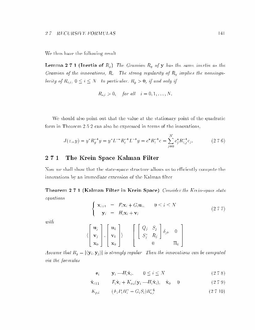
��� RECURSIVE FORMULAS ��
We thus have the following result�
Lemma ����� �Inertia of Ry� The Gramian Ry of y has the same inertia as the
Gramian of the innovations� Re� The strong regularity of Ry implies the nonsingu�
larity of Re�i� � � i � N � In particular� Ry � �� if and only if
Re�i � �� for all i � �� �� � � � � N�
We should also point out that the value at the stationary point of the quadratic
form in Theorem ����� can also be expressed in terms of the innovations�
J�zo� y� � y�R��y y � y�L��R��e L��y � e�R��e e �NXj��
e�jR��e�j ej� ������
���� The Krein Space Kalman Filter
Now we shall show that the state�space structure allows us to e�ciently compute the
innovations by an immediate extension of the Kalman �lter�
Theorem ����� �Kalman Filter in Krein Space� Consider the Krein�space state
equations ���xi�� � Fixi �Giui� � � i � N
yi � Hixi � vi�����
with
h
� �uj
vj
x�
����� �
� �uk
vk
x�
�����i �
� �
�� Qj Sj
S�j Rj
�� �jk �
� ��
�����
Assume that Ry � �hyi�yji is strongly regular� Then the innovations can be computed
via the formulas
ei � yi �Hi"xi� � � i � N ������
"xi�� � Fi"xi �Kp�i�yi �Hi"xi�� "x� � � ������
Kp�i � �FiPiH�i �GiSi�R
��e�i �������

�� CHAPTER �� LINEAR ESTIMATION IN KREIN SPACES
where
Re�i � hei� eii � Ri �HiPiH�i
and the fPig can be recursively computed via the Riccati recursion
Pi�� � FiPiF�i �Kp�iRe�iK
�p�i �GiQiG
�i � P� � ��� �������
The number of computations is dominated by those in ����� and is readily seen to
be O�n�� per iteration�
Remark� The only di�erence from the conventional Kalman �lter expressions is that
the matrices Pi and Re�i �and� by assumption� ��� Qi and Ri� may now be inde�nite�
Proof� The same as in the usual Kalman �lter theory �see� e�g�� �Kai�� �� However�
for completeness and to show the power of the geometric viewpoint� we present a
simple derivation� There is absolutely no formal di�erence between the steps in the
�usual� Hilbert space case and in the Krein space case�
Begin by noting that
ei � yi � "yi � yi � �Hi"xi � "vi� � yi �Hi"xi � Hi#xi � vi �������
where "xi is the projection of xi on Lfy�� � � � �yi��g and where we have de�ned #xi �
xi � "xi� It follows readily that
Re�i � hei� eii � Ri �HiPiH�i � Pi
�� h#xi� #xii� �������
Recall �see Lemma ����� that the strong nonsingularity �all leading minors non�zero�
of Ry implies that the fRe�ig are nonsingular �rather than positive�de�nite� as in
the Hilbert space case�� The Kalman �lter can now be readily derived by using the
orthogonality of the innovations and the state�space structure� Thus we �rst write
"xi��ji � "xi�� �iX
j��
hxi��� ejihej� eji��K ej�
and to seek a recursion we decompose the above as
"xi�� �i��Xj��
hxi��� ejiR��e�j ej �Kp�iei� Kp�i�� hxi��� eiiR��e�i �

��� RECURSIVE FORMULAS ��
Now
hxi��� eii � Fihxi� eii �Gihui� eii� Fihxi�Hi#xi � vii �Gihui�Hi#xi � vii� Fih#xi�Hi#xii� � � � �Gihui�vii � FiPiH
�i �GiSi�
Note also that the �rst summation can be rewritten as
Fii��Xj��
hxi� ejiR��e�j ej �Gi
i��Xj��
hui� ejiR��e�j ej � Fi"xi � �
Combining these facts we �nd
"xi�� � Fi"xi �Kp�iei ������
and
Kp�i � �FiPiH�i �GiSi�R
��e�i � �������
It now remains to �nd a recursion for Pi� To this end� note that if we de�ne the
Gramians �i � hxi�xii and �i � h xi� xii� then the orthogonality of the "xi and #xi
yields�
Pi � �i � �i�
The state�space equation ������� shows that the state variance �i� obeys the recursion
�i�� � Fi�iF�i �GiQ
�iG
�i �
Likewise� the orthogonality of the innovations implies that ������ will yield
�i�� � Fi�iF�i �Kp�iRe�iK
�p�i� �� � ��
Subtracting the above two equations yields the desired Riccati recursion for Pi�
Pi�� � FiPiF�i �GiQiG
�i �Kp�iRe�iK
�p�i� P� � ��� �������
Equations ������� to ������� constitute the Kalman �lter of Theorem �����
In Kalman �lter theory there are many variations of the above formulas and we
note one here� Let us de�ne the �ltered estimate� xiji as the projection of xi onto
Lfy�� � � � �yig�

� CHAPTER �� LINEAR ESTIMATION IN KREIN SPACES
Theorem ����� �Measurement and Time Updates� Consider the Krein state�
space equations of Theorem ��� and assume that Ry is strongly regular� Then when
Si � �� the �ltered estimates "xiji can be computed via the following �measurement and
time update� formulas
"xi��ji�� � "xi�� �Kf�i��ei��� "x� � �� Kf�i�� � Pi��H�i��R
��e�i�� ������
"xi�� � Fi"xiji �������
where ei� Re�i and Pi are as in Theorem ����
Corollary ����� �Filtered Recursions� The two step recursions of Theorem ���
can be combined into the single recursion
"xi��ji�� � Fi"xiji �Kf�i���yi�� �Hi��Fi"xiji�� "x��j�� � �� �������
For numerical reasons� certain square�root versions of the KF are now more often
used in state�space estimation� Furthermore for constant systems� or in fact for sys�
tems where the time�variation is structured in a certain way� the Riccati recursions
and the square�root recursions� both of which take O�n�� elementary computations
��ops� per iteration can be replaced by the more e�cient Chandrasekhar recursions�
which require only O�n�� �ops per iteration �MSK� SK�a � The square�root and
Chandrasekhar recursions can both be extended to the Krein space setting� as de�
scribed in �HSK�c � and as we shall see in Chapter ��
Before closing this section we shall note how the innovations computed in Theo�
rem ���� can be used to determine the projections "x�jN and "ujN using the formulas
�����and �������
Lemma ����� �Computation of Inner Products� We can write
hx�� eii � ��%�F�KH�i� ��H
�i �������
and
huj� eii ����QjG
�j%
�F�KH�i� j � ��H�
i � Si�ij j � i
� j � i�������

��� RECURSIVE FORMULAS ��
where
%F�KH�i� j���
i��Yk�j
�Fk �Kp�kHk��
These lead to the recursions�
"x�ji � "x�ji�� ���%�F�KH �i� ��H
�i R
��e�i ei� "x�j�� � � �������
and
"ujji �
���
"ujji�� �QjG�j%
�F�KH �i� j � ��H�
i R��e�i ei� "ujjj � SjR
��e�j ei j � i
� j � i�������
where %�F�KH�i� j� �i � j� satis�es the recursion
%�F�KH �i� �� j� � %�F�KH�i� j��Fi �Kp�iHi��� %�F�KH �j� j� � I�
Proof� Straightforward computation�
���� Recursive State�Space Estimation and Quadratic Forms
Theorems ���� and ��� below are essentially restatements of Theorems ����� and
������ when a state space model is assumed� and a recursive solution is sought�
The error Gramian associated with the problem of projecting fx��ug onto Lfyghas already been identi�ed in Lemma ������ and ������������� furnishes a recursive
procedure for calculating this projection� The condition for a minimum is Ry � ��
where Ry has been shown to be congruent to the diagonal matrix Re� This gives the
following theorem�
Theorem ���� �Stochastic Problem� Suppose z � colfx��ug and y are related
through the state�space model ������ and ������� and that Ry is strongly regular�

�� CHAPTER �� LINEAR ESTIMATION IN KREIN SPACES
Then the state�space estimation algorithm ���������� recursively computes the
stationary point of the error Gramian
hz� k�y� z� k�yi
over all k�y� Moreover this stationary point is a minimum if and only if
Re�j � � for j � �� � � � � i�
Similarly� the scalar quadratic form associated with the �partially� equivalent de�
terministic problem has already been identi�ed in Lemma ������
JN�x�� u� y� � x������ x� �
XN
j��
hu�j �yj �Hjxj��
i �� Qj Sj
S�j Rj
���� �� uj
yj �Hjxj
�� �
������
In particular� "x�jN and "ujjN are the stationary points of JN�x�� u� y� over x� and uj�
and subject to the state�space constraints xj�� � Fjxj � Gjuj� j � �� � � � � N � In the
recursions� for each time i� we �nd "x�ji and "ujji� which are the stationary points of
Ji�x�� u� y� � x������ x� �
Xi
j��
hu�j �yj �Hjxj��
i �� Qj Sj
S�j Rj
���� �� uj
yj �Hjxj
�� �
�������
Theorem ���� �Deterministic Problem� If Ry is strongly regular� the station�
ary point of the quadratic form
Ji�x�� u� y� � x������ x� �
Xi
j��
hu�j �yj �Hjxj��
i �� Qj Sj
S�j Rj
���� �� uj
yj �Hjxj
��
�������
over x� and uj� subject to the state�space constraints xj�� � Fjxj�Gjuj� j � �� �� � � � � i
can be recursively computed as
"x�ji � "x�ji�� ���%�F�KH�i� ��H
�i R
��e�i ei� "x�j�� � �

��� RECURSIVE FORMULAS �
and
"ujji �
���
"ujji�� �QjG�j%
�F�KH �i� j � ��H�
i R��e�i ei� "ujjj � SjR
��e�j ei j � i
� j � i
where the innovations ej can be computed via the recursions
"xi�� � Fi"xi �Kp�iei� "x� � �
with Kp�i � �FiPiH�i �GiSi�R
��e�i � Re�i � Ri�HiPiH
�i � ei � yi�Hi"xi� and Pi satisfying
the Riccati recursion
Pi�� � FiPiF�i �GiQiG
�i �Kp�iR
��e�iK
�p�i � P� � ���
Moreover� the value of Ji�x�� u� y� at the stationary point is given by
Ji�"x�ji� "uji� y� �iX
j��
e�jR��e�j ej�
Proof� The proof follows from the basic equivalence between the deterministic and
stochastic problems� The recursions for "x�ji and "ujji are the same as those in the
stochastic problem of Lemma ����� and the innovations ei are found via the Krein
space Kalman �lter of Theorem �����
As mentioned earlier� the deterministic quadratic form of Theorem ��� is often
encountered in estimation problems� By appeal to Gaussian assumptions on the vi� ui
and x�� and maximum likelihood arguments� it is well�known that state estimates can
be obtained via a deterministic quadratic minimization problem� Here we have shown
this result using simple projection arguments� and have generalized it to inde�nite
quadratic forms�
The result of Theorem ��� is probably the most important result of this paper�
and we shall make frequent use of it in the next two chapters to solve the problems
of H� and risk�sensitive estimation� and �nite�memory adaptive �ltering� In those
problems we shall also need to recursively check for the condition for a minimum� and
therefore we will now study these conditions in more detail�

�� CHAPTER �� LINEAR ESTIMATION IN KREIN SPACES
Recall from Lemma ���� that the above deterministic problem has a minimum if�
and only if� Ry and R� S�Q��S have the same inertia� Since Ry is congruent to the
block diagonal matrix Re� and since R� S�Q��S is also block diagonal� the solution
of the recursive stationarization problem will give a minimum at each step if and only
if all the block diagonal elements of Re and R�S�Q��S have the same inertia� This
leads to the following result�
Lemma ���� �Inertia Conditions for a Minimum� If �� � �� Q � � and R is
non�singular� then the �unique� stationary points of the quadratic forms ������� for
i � �� �� � � � N � will each be a unique minimum if� and only if� the matrices
Re�j and Rj � S�jQ��j Sj
have the same inertia for all j � �� �� � � � N � In particular� when Sj � �� the condition
becomes that Re�j and Rj should have the same inertia for all j � �� �� � � � N �
The conditions of the above Lemmaare easy to check since the Krein space Kalman
�lter used to compute the stationary point also computes the matrices Re�j� There
is another condition� more frequently quoted in the H� literature� which we restate
here �see e�g� � �ST�� ��
Lemma ���� �Condition for a Minimum� If �� � �� Q � �� R is invertible�
Q � SR��S� � � andhFj Gj
ihas full rank for all j� then the quadratic forms
������ will each have a unique minimum if� and only if�
P��jjj � P��j �H�jR
��j Hj � � j � �� �� ���� N�
It also follows in the minimum case that Pj�� � � for j � �� �� ���� N �
Remark� In comparison to our result in Lemma ����� we here have the additional
requirement that thehFj Gj
imust be full rank� Furthermore� we not only have
to compute the Pj �which is done via the Riccati recursion of the Kalman �lter�� but
we also have to invert Pj �and Rj� at each step and then check for the positivity of
P��j � H�jR
��j Hj � The test of Lemma ���� uses only quantities already present in
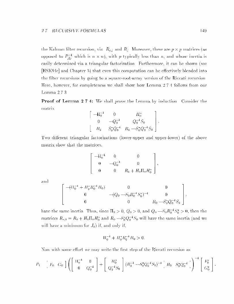
��� RECURSIVE FORMULAS ��
the Kalman �lter recursion� viz� Re�j and Rj � Moreover� these are p� p matrices �as
opposed to P��jjj which is n � n�� with p typically less than n� and whose inertia is
easily determined via a triangular factorization� Furthermore� it can be shown �see
�HSK�c and Chapter �� that even this computation can be e�ectively blended into
the �lter recursions by going to a square�root�array version of the Riccati recursion�
Here� however� for completeness we shall show how Lemma ��� follows from our
Lemma �����
Proof of Lemma ����� We shall prove the Lemma by induction� Consider the
matrix � ������ � H�
�
� �Q��� Q��� S�
H� S��Q��� R� � S��Q
��� S�
����� �
Two di�erent triangular factorizations �lower�upper and upper�lower� of the above
matrix show that the matrices�
� ������ � �
� �Q��� �
� � R� �H���H��
����� �
and � ������� �H�
�R��� H�� � �
� ��Q� � S�R��� S���
�� �
� � R� � S��Q��� S�
����� �
have the same inertia� Thus� since �� � �� Q� � �� and Q� � S�R��� S�� � �� then the
matrices Re�� � R� �H���H�� and R� � S��Q
��� S� will have the same inertia �and we
will have a minimum for J�� if� and only if�
���� �H��R
��� H� � ��
Now with some e�ort we may write the �rst step of the Riccati recursion as
P� �hF� G�
i���� ��� �
� Q���
��
�� H�
�
Q��� S�
�� �R��� � S��Q
��� S��
��hH� S��Q
���
i�A�� �� F ��
G��
�� �

��� CHAPTER �� LINEAR ESTIMATION IN KREIN SPACES
Moreover� the center matrix appearing in the above expression is congruent to�� ���� �H�
�R��� H� �
� �Q� � S�R��� S���
��
�� �
and hence is positive de�nite� Thus ifhF� G�
ihas full rank� we can conclude that
P� � �� We can now repeat the argument for the next time instant and so on�
We close this section with yet another condition which will be useful in control
problems�
Lemma ����� �Condition for a Minimum� If in addition to the conditions of
Lemma ����� the matrices Fj � GjSjR��j Hj are invertible for all j� then the de�
terministic problems of Theorem ���� will each have a unique minimum if� and only
if� PN�� � � and
�Qj � SjR��j S�j �
�� �G�jP��j��Gj � � j � �� �� ���� N�
Proof� Let us �rst note that the Riccati recursion can be rewritten as
Pi�� � FiPiF�i �GiQiG
�i � �FiPiH
�i �GiSi��Ri �HiPiH
�i ����FiPiH
�i �GiSi�
�
� �Fi �GiSiR��i Hi�Pi�Fi �GiSiR
��i Hi�
� �Gi�Qi � SiR��i S�i �G
�i
��Fi �GiSiR��i Hi�PiH
�i �Ri �HiPiH
�i ���HiPi�Fi �GiSiR
��i Hi�
�
� �Fi �GiSiR��i Hi��P
��i �H�
i R��i Hi�
���Fi �GiSiR��i Hi�
� �Gi�Qi � SiR��i S�i �G
�i �
The proof� which uses the last of the above equalities� now follows from the following
sequence of congruences and Lemma ������ Pi�� �
� �Qi � SiR��i S�i �
�� �G�iP��i��Gi
��
��� Pi�� Gi
G�i �Qi � SiR��i S�i �
��
��
��� Pi�� �Gi�Qi � SiR
��i S�i �G
�i �
� �Qi � SiR��i S�i �
��
��

��� CONCLUDING REMARKS ���
�
�� �Fi �GiSiR
��i Hi��P
��i �H�
i R��i Hi����Fi �GiSiR
��i Hi�� �
� �Qi � SiR��i S�i �
��
��
��� �P��i �H�
i R��i Hi��� �
� �Qi � SiR��i S�i �
��
�� �
��� Concluding Remarks
We developed a self�contained theory for linear estimation in Krein spaces� We started
with the notion of projections and discussed their relation to stationary points of
certain quadratic forms encountered in a pair of partially equivalent stochastic deter�
ministic problems� By assuming an additional state�space structure� we showed that
projections could be recursively computed by a Krein space Kalman �lter� several
applications for which are described in the next chapters�
The approach� in all these applications� is that given an inde�nite deterministic
quadratic form� to which H�� risk�sensitive� and �nite�memory problems lead almost
by inspection� one can relate them to a corresponding Krein space stochastic problem
for which the Kalman �lter can be written down immediately and used to obtain
recursive solutions of the above problems�

��� CHAPTER �� LINEAR ESTIMATION IN KREIN SPACES
��A Proof of the TimeVariant KYP Lemma
In this section we give a stochastic proof and geometric interpretation of the time�
variant Kalman�Yakubovich�Popov �KYP� Lemma whose steady�state counterpart
was introduced in Sec� ������ The method is based on considering linear time�variant
systems driven by processes with elements in a Krein space rather than the usual
Hilbert space setting�
��A�� Statement of the Lemma
Theorem ��A�� �Time�Variant KYP Lemma� Consider the observable linear time�
variant state�space model
���xi�� � Fixi � ui� � � i � N
yi � Hixi � vi
with h
� �x�
ui
vi
����� �
� �x�
ui
vi
�����i �
� �
�� � �
� Qi�ij Si�ij
� S�i �ij Ri�ij
������ Then the following two statements
are equivalent�
�i� The output spectrum is positive semi�de�nite� i�e�
Ry � ��
�ii� There exists a sequence of Hermitian matrices fZigN��i�� � such that
�� � Z� � � ���A���
and
�� �Zi�� � FiZiF
�i �Qi Si � FiZiH
�i
S�i �HiZiF�i Ri �HiZiH
�i
�� � �� i � �� �� � � � � N� ���A���
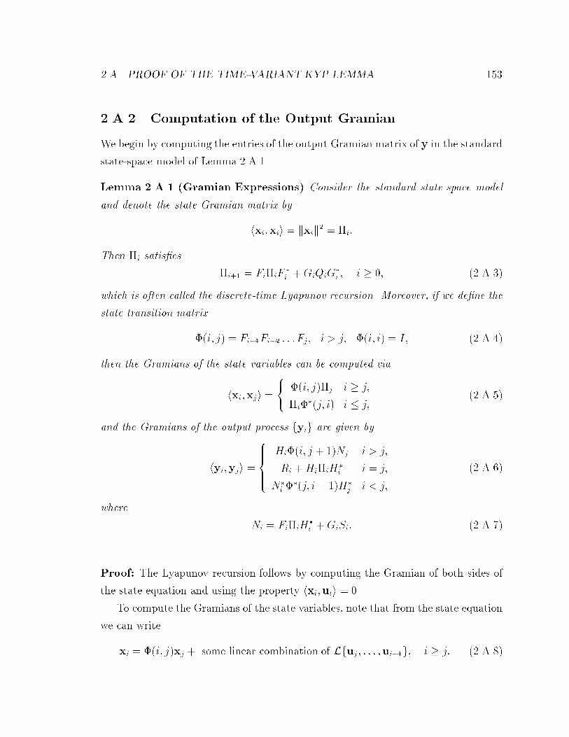
��A� PROOF OF THE TIME�VARIANT KYP LEMMA ���
��A�� Computation of the Output Gramian
We begin by computing the entries of the output Gramian matrix of y in the standard
state�space model of Lemma ��A���
Lemma ��A�� �Gramian Expressions� Consider the standard state�space model
and denote the state Gramian matrix by
hxi�xii � kxik� � �i�
Then �i satis�es
�i�� � Fi�iF�i �GiQiG
�i � i � �� ���A���
which is often called the discrete�time Lyapunov recursion� Moreover� if we de�ne the
state transition matrix
%�i� j� � Fi��Fi�� � � � Fj� i � j� %�i� i� � I� ���A��
then the Gramians of the state variables can be computed via
hxi�xji ����
%�i� j��j i � j�
�i%��j� i� i � j����A���
and the Gramians of the output process fyig are given by
hyi�yji �
���������
Hi%�i� j � ��Nj i � j�
Ri �Hi�iH�i i � j�
N�i %
��j� i� ��H�j i � j�
���A���
where
Ni � Fi�iH�i �GiSi� ���A��
Proof� The Lyapunov recursion follows by computing the Gramian of both sides of
the state equation and using the property hxi�uii � ��
To compute the Gramians of the state variables� note that from the state equation
we can write
xi � %�i� j�xj � some linear combination of Lfuj � � � � �ui��g� i � j� ���A���

�� CHAPTER �� LINEAR ESTIMATION IN KREIN SPACES
Therefore�
hxi�xji � %�i� j�hxj�xji� �� for i � j�
Next note that
for i � j� hxi�xji � hxj �xii� � �i%��j� i�� ���A���
Finally� we note that
hyi�yji � Hihxi�xjiH�i �Hihxi�vji� hvi�xjiH�
j � hvi�vji� ���A����
Now for i � j� the last two terms on the RHS are zero� while the second term is�
hxi�xji � %�i� j � ��Gjhui�vji � %�i� j � ��GjSj � ���A����
and the �rst term is
hxi�xji � %�i� j��j � %�i� j � ��Fj�j� ���A����
Collecting these results gives the �rst of the desired expressions for hyi�yji� The
remaining two �for i � j and i � j� follow in similar fashion�
The above Lemma allows us to computes the entries of the output Gramian Ry�
It is also possible to give the following global expression of the output Gramian�
Ry � O��O� �h& I
i �� Q S
S� R
���� &�
I
�� ���A����
where
Q � diag�Q�� � � � � QN� � R � diag�R�� � � � � RN� � S � diag�S�� � � � � SN �
and where we have de�ned the observability map
O �� O��� N� �
� �
H�%��� ��
H�%��� ��
H�%��� �����
HN%�N� ��
������������
�
� �
H�
H�F�
H�F�F�
���
HNFN�� � � � F�
������������
� ���A���
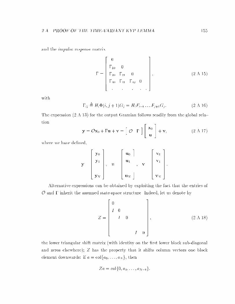
��A� PROOF OF THE TIME�VARIANT KYP LEMMA ���
and the impulse response matrix
& �
� �
�
&�� �
&�� &�� �
&�� &�� &�� �
� � � � �
������������ ���A����
with
&ij�� Hi%�i� j � ��Gj � HiFi�� � � � Fj��Gj � ���A����
The expression ���A���� for the output Gramian follows readily from the global rela�
tion
y � Ox� � &u � v �hO &
i �� x�
u
��� v� ���A���
where we have de�ned�
y �
� �
y�
y����
yN
���������� u �
� �
u�
u����
uN
���������� v �
� �
v�
v����
vN
����������
Alternative expressions can be obtained by exploiting the fact that the entries of
O and & inherit the assumed state�space structure� Indeed� let us denote by
Z �
� �
�
I �
I �� � �
� � �
I �
������������
� ���A����
the lower triangular shift matrix �with identity on the �rst lower block sub�diagonal
and zeros elsewhere�� Z has the property that it shifts column vectors one block
element downwards� if a � colfa�� � � � � aNg� then
Za � colf�� a�� � � � � aN��g�

��� CHAPTER �� LINEAR ESTIMATION IN KREIN SPACES
Using the shift matrix Z� we can rewrite the ith �block� column of the impulse
response matrix as �refer to Eqs� ���A�������A���� where the structure of & is shown�
i�th column of & � Z i
� �
�
Hi%�i� i�
Hi��%�i� �� i����
HN%�N� i�
������������
Gi� ���A����
Consequently� the following expressions for Ry also result�
Lemma ��A�� �Two Expressions for the Output Gramian� The output Gramian�
Ry� corresponding to the standard state�space model can be written in either of the
following two forms�
�i�
Ry �NXi��
Z i
� �
� I
Hi%�i� i� �
Hi��%�i� �� i� ����
���
HN%�N� i� �
������������
�� � Ni
N�i Ri �Hi�iH
�i
��
� �
� I
Hi%�i� i� �
Hi��%�i� �� i� ����
���
HN%�N� i� �
������������
�
Z�i�
���A����
�ii�
Ry � O��O��NXi��
Z i
� �
� I
Hi%�i� i� �
Hi��%�i� �� i� ����
���
HN%�N� i� �
������������
�� Qi Si
S�i Ri
��
� �
� I
Hi%�i� i� �
Hi��%�i� �� i� ����
���
HN%�N� i� �
������������
�
Z�i�
���A����
Proof� The proof of �i� follows from inspection of the expressions ���A��� for the
elements of Ry� Likewise �ii� follows by inspecting ���A���� and using ���A�����
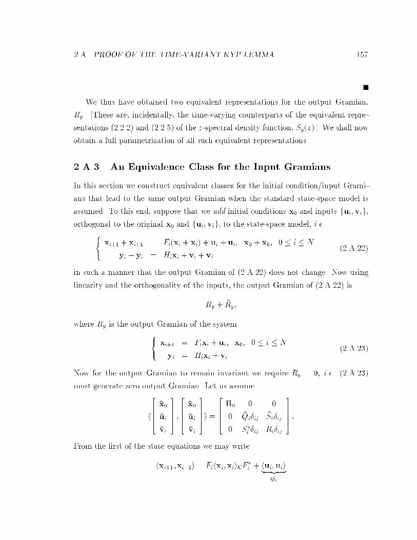
��A� PROOF OF THE TIME�VARIANT KYP LEMMA ��
We thus have obtained two equivalent representations for the output Gramian�
Ry� �These are� incidentally� the time�varying counterparts of the equivalent repre�
sentations ������� and ������� of the z�spectral density function� Sy�z�� We shall now
obtain a full parametrization of all such equivalent representations�
��A�� An Equivalence Class for the Input Gramians
In this section we construct equivalent classes for the initial condition(input Grami�
ans that lead to the same output Gramian when the standard state�space model is
assumed� To this end� suppose that we add initial conditions �x� and inputs f�ui� �vig�orthogonal to the original x� and fui�vig� to the state�space model� i�e�
���xi�� � �xi�� � Fi�xi � �xi� � ui � �ui� x� � �x�� � � i � N
yi � �yi � Hixi � vi � �vi���A����
in such a manner that the output Gramian of ���A���� does not change� Now using
linearity and the orthogonality of the inputs� the output Gramian of ���A���� is
Ry � �Ry�
where �Ry is the output Gramian of the system���
�xi�� � Fi�xi � �ui� �x�� � � i � N
�yi � Hi�xi � �vi���A����
Now for the output Gramian to remain invariant we require �Ry � �� i�e� ���A����
must generate zero output Gramian� Let us assume
h
� �
�x�
�ui
�vi
����� �
� �
�x�
�ui
�vi
�����i �
� �
��� � �
� �Qi�ij �Si�ij
� �S�i �ij �Ri�ij
����� �
From the �rst of the state equations we may write
hxi���xi��i � Fihxi�xiiKF �i � hui�uii �z ��Qi

��� CHAPTER �� LINEAR ESTIMATION IN KREIN SPACES
so that if we de�ne Zi � �hxi�xii� we have
�Qi � �Zi�� � FiZiF�i � ���A���
Now
h�yi� �yii � Hihxi�xiiH�i � �Ri � �HiZiH
�i � �Ri � � ���A����
and for j � �
h�yi�j � �yii � Hi�jFi�j�� � � � Fi����FiZiH�i � �Si� � ��
If we write the above equation for all j � ��� �
Hi��
Hi��Fi��
Hi��Fi��Fi�����
�����������FiZiH
�i � �Si� � �
and since we have assumed the observability of the system� the matrix on the left�hand
side is full rank� so that
�Si � FiZiH�i � ���A����
Combining ���A���� ���A���� and ���A���� yields
��� � �Z� and
�� �Qi
�Si�S�i �Ri
�� �
�� �Zi�� � FiZiF
�i FiZiH
�i
HiZiF�i HiZiH
�i
�� �
It is now straightforward to show the following Lemma�
Lemma ��A� �Equivalent Class for Input Gramians� �a� The output Gramian�
Ry� of the state�space model���xi�� � Fixi � ui� � � i � N
yi � Hixi � vi���A���
with h
� �x�
ui
vi
����� �
� �x�
ui
vi
�����i �
� �
�� � �
� Qi�ij Si�ij
� S�i �ij Ri�ij
����� is invariant under the transfor�
mation
�� � �� � Z� and
�� Qi Si
S�i Ri
���
�� �Zi�� � FiZiF
�i �Qi FiZiH
�i � Si
HiZiF�i � S�i HiZiH
�i �Ri
��

��A� PROOF OF THE TIME�VARIANT KYP LEMMA ���
for any sequence of Hermitian matrices fZigN��i�� �
�b� If the system ��A��� is observable� and there exist����
�� �
�� Q
�i S
�i
S��i R
�i
����� and
����
�� �
�� Q
�i S
�i
S��i R
�i
�����
that yield identical output Gramians� i�e��
R�y � R�
y �
then there exists a unique sequence of Hermitian matrices fZigN��i�� such that
��� � �
�� �Z� and
�� Q
�i S
�i
S��i R
�i
�� �
�� �Zi�� � FiZiF
�i �Q
�i FiZiH
�i � S
�i
HiZiF�i � S
��i HiZiH
�i �R
�i
�� �
Proof� We have already shown part �a� prior to the statement of the lemma�
We therefore proceed to prove part �b�� To this end� suppose that there exist
f��� � fQ�
i � R�i � S
�i gg and f��
� � fQ�i � R
�i � S
�i gg that yield the same Ry� and de�
�ne the unique sequences of matrices� fZ�i � N
�i � R
���ig and fZ�
i � N�i � R
���ig� via the
recursions����Z�i�� � FiZ
�i F �i �Q
�i � N
�i � FiZ
�i H�
i � S�i � R
���i � R
�i �HiZ
�i H�
i
Z�i�� � FiZ
�i F �i �Q
�i � N
�i � FiZ
�i H�
i � S�i � R
���i � R
�i �HiZ
�i H�
i
���A����
initialized with Z�� � Z
�� � ��� Using the result of Lemma ��A��� part �i�� this
means that we can write
Ry �NXi��
Z i
� �
� I
Hi%�i� i� �
Hi��%�i� �� i� ����
���
HN%�N� i� �
������������
�� � N
ji
N�ji R
j��i
��
� �
� I
Hi%�i� i� �
Hi��%�i� �� i� ����
���
HN%�N� i� �
������������
�
Z�i
�NXi��
Z i
� �
�
Hi%�i� i�Nji
Hi��%�i� �� i�N ji
���
HN%�N� i�Nji
������������
� diag�Rj���� � � � � R
j��N� �
�� strictly upper
triangular matrix
��

��� CHAPTER �� LINEAR ESTIMATION IN KREIN SPACES
for j � �� �� The above expression allows us to identify the i�th block diagonal entry
of Ry as R���i � R
���i � Ry�ii� and the strictly lower triangular �i� j��th block entry as�
Hi%�i� j�N�j � Hi%�i� j�N
�j � Ry�ij �
The observability of the system allows us to conclude that N �i � N
�i � Therefore
�� � N
�i
N��i R
���i
�� �
�� � N
�i
N��i R
���i
��
or� equivalently��� �Z
�i�� � FiZ
�i F �i �Q
�i FiZ
�i H�
i � S�i
HiZ�i F �i � S
��i R
�i �HiZ
�i H�
i
�� �
�� �Z
�i�� � FiZ
�i F �i �Q
�i FiZ
�i H�
i � S�i
HiZ�i F �i � S
��i R
�i �HiZ
�i H�
i
�� �
from which we conclude that the unique sequence of matrices� fZi�� Z
�i �Z
�i gN��
i��
relates the two sets of input Gramians�
��A�� The Proof
We can now proceed with the proof of the KYP Lemma� First note that the in view
of Lemma ��A��� part �ii�� and Lemma ��A��� part �a�� going from �ii� to �i� in the
KYP Lemma ��A�� is trivial� Therefore we shall focus on the other direction � from
�i� to �ii��
To this end� suppose that Ry � �� If this is the case� then Ry will admit the
following unique block lower�diagonal�upper factorization���
Ry � LReL�� ���A����
where L is block lower diagonal with block unit diagonal� and Re is block diagonal
with
Re � �� ���A����
��This factorization is� of course� related to the Cholesky factorization of positive semide�nitematrices �see e�g�� �GL��� HJ��� Str���
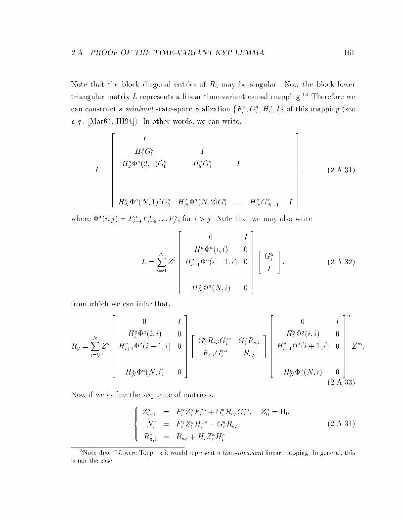
��A� PROOF OF THE TIME�VARIANT KYP LEMMA ���
Note that the block diagonal entries of Re may be singular� Now the block lower
triangular matrix L represents a linear time�variant causal mapping��� Therefore we
can construct a minimal state�space realization fF ai � G
ai �H
ai � Ig of this mapping �see
e�g�� �Mar�� HI� �� In other words� we can write�
L �
� �
I
Ha�G
a� I
Ha�%
a��� ��Ga� Ha
�Ga� I
���� � �
HaN%
a�N� ��aGa� Ha
N%a�N� ��Ga
� � � � HaNG
aN�� I
���������������
� ���A����
where %a�i� j� � F ai��F
ai�� � � � F
aj � for i � j� Note that we may also write
L �NXi��
Z i
� �
� I
Hai %
a�i� i� �
Hai��%
a�i� �� i� ����
���
HaN%
a�N� i� �
������������
�� Ga
i
I
�� � ���A����
from which we can infer that�
Ry �NXi��
Z i
� �
� I
Hai %
a�i� i� �
Hai��%
a�i� �� i� ����
���
HaN%
a�N� i� �
������������
�� Ga
iRe�iGa�i Ga
iRe�i
Re�iGa�i Re�i
��
� �
� I
Hai %
a�i� i� �
Hai��%
a�i� �� i� ����
���
HaN%
a�N� i� �
������������
�
Z�i�
���A����
Now if we de�ne the sequence of matrices����������
Zai�� � F a
i Zai F
a�i �Ga
iRe�iGa�i � Za
� � ��
Nai � F a
i Zai H
a�i �Ga
iRe�i
Ra��i � Re�i �HiZ
ai H
�i
���A���
��Note that if L were Toeplitz it would represent a time�invariant linear mapping In general� thisis not the case

��� CHAPTER �� LINEAR ESTIMATION IN KREIN SPACES
then using an argument similar to the one presented in the proof of Lemma ��A��
allows us to conclude that the diagonal entries of Ry are
Ry�ii � Re�i �HiZai H
�i � ���A����
and that the strictly lower triangular entries of Ry are
Ry�ij � Hai %
a�i� j�Naj � i � j� ���A����
Had we� instead of the representation ���A���� for Ry� used the representation of
Lemma ��A��� part �ii�� then we would have identi�ed the entries of Ry as
���
Ry�ii � Ri �HiZiH�i
Ry�ij � Hi%�i� j�Nj� i � j���A���
where ���������
Zi�� � FiZiFa�i � Qi� Z� � ��
Ni � FiZiH�i � Si
R��i � Ri �HiZiH�i
� ���A����
Equating these two results yields�
Re�i �HiZai H
�i � Ri �HiZiH
�i � ���A����
and
Hai %
a�i� j�Naj � Hi%�i� j�Nj� i � j� ���A���
This latter expression means that the two systems with state�space representations�
fF ai � N
ai �H
ai g and fFi� Ni�Hig have the same impulse response matrix �or input�
output map�� Thus there must exist a �possibly time�variant� similarity transforma�
tion� Ti� such that �����������������������
�� F i
a �� F a�c
i
�� � T��i FiTi
�� Na
i
�
�� � T��i Ni
hHai Ha�c
i
i� HiTi
� ���A���

��A� PROOF OF THE TIME�VARIANT KYP LEMMA ���
where the superscript )c$ represents the uncontrollable states of the system fFi� Ni�Hig��Note that we have no unobservable modes since fF�Hg is assumed observable� On
the other hand� we can write
Hai %
a�i� j�Gaj �
hHai Ha�c
i
i i��Yk�j
�� F i
a �� F a�c
i
���� Ga
i
�
��
� Hi%�i� j�Tj
�� Ga
i
�
��
�z �Kp�j
�
But using ���A����� this implies that
Ry �NXi��
Z i
� �
� I
Hi%�i� i� �
Hi��%�i� �� i� ����
���
HN%�N� i� �
������������
�� Kp�iRe�iK
�p�i Kp�iRe�i
Re�iK�p�i Re�i
��
� �
� I
Hi%�i� i� �
Hi��%�i� �� i� ����
���
HN%�N� i� �
������������
�
Z�i�
���A���
Comparing the above representation of Ry with that given in Lemma ��A��� part �ii��
indicates that there must exist a unique sequence of Hermitian matrices� say f �ZigN��i�� �
such that
�� � �Z� � �� ���A���
and�� � �Zi�� � Fi �ZiF
�i �Qi Si � Fi �ZiH
�i
S�i �Hi�ZiF
�i Ri �Hi
�ZiH�i
�� �
�� Kp�iRe�iK
�p�i Kp�iRe�i
Re�iK�p�i Re�i
�� � ��
���A��
where we have used the fact that Re�i � �� But this is the desired result�
��A�� Geometric Interpretation
Since we motivated and introduced the KYP lemma by considering state�space models
whose inputs were elements of a Krein space� it seems natural to suspect that the
KYP Lemma should admit further interpretation� or a simpler proof� in the context

�� CHAPTER �� LINEAR ESTIMATION IN KREIN SPACES
of Krein spaces� We shall presently see that this is indeed the case� and that the KYP
Lemma has a simple geometric interpretation in terms of a certain decomposition in
Krein space�
The Geometric Setup
Since our interpretation of the KYP Lemma will use Krein space geometry� we begin
by carefully de�ning the spaces in which our inputs and outputs lie�
The initial condition(input space� Kd� consists of all initial conditions� x�� and all
input sequences� fui�vig� that are orthogonal to one another and that have �possibly
inde�nite� arbitrary Gramian matrices� �� and
�� Qi Si
S�i R
��� Thus� we may write
Kd �
�����������������������������������
� �
x�
u����
uN
v����
vN
������������������
j h
� �x�
ui
vi
����� �
� �x�
uj
vj
�����i �
� �
�� � �
� Qi�ij Si�ij
� S�i �ij Ri�ij
�����
�����������������������������������
� ���A���
Note that Kd� and Kd
� have the obvious structures�
Kd� �
�����������������������������������
� �
x�
u����
uN
v����
vN
������������������
j h
� �x�
ui
vi
����� �
� �x�
uj
vj
�����i �
� �
�� � �
� Qi�ij Si�ij
� S�i �ij Ri�ij
����� � �
�����������������������������������
�

��A� PROOF OF THE TIME�VARIANT KYP LEMMA ���
�
�
�
�
�
�
�
�
�
�
Kd� Ks
�
Ks�Kd
�
hO � I
i
Kd Ks
Figure ���� Mapping from input space to output space�
and
Kd� �
�����������������������������������
� �
x�
u����
uN
v����
vN
������������������
j h
� �x�
ui
vi
����� �
� �x�
uj
vj
�����i �
� �
�� � �
� Qi�ij Si�ij
� S�i �ij Ri�ij
����� � �
�����������������������������������
�
To now construct the output space� consider the time�variant state�space model���xi�� � Fixi � ui� � � i � N
yi � Hixi � vi���A���
where x� and the fui�vig belong to Kd� Now if� as before� we de�ne
y � colfy�� � � � �yNg � u � colfu�� � � � �uNg � v � colfv�� � � � �vNg
then we can write
y � Ox� � &u � v �hO & I
i� �x�
u
v
����� � ���A��

��� CHAPTER �� LINEAR ESTIMATION IN KREIN SPACES
Thus� the y also form a Krein space� Ks� We can formally represent this Krein space
as
y Ks �hO & I
iKd�
and in particular Ks � Ks� �Ks
� � with
Ks� �
hO & I
iKd
� and Ks� �
hO & I
iKd� � ���A���
Thus� Ks is the Krein space of all possible outputs of ���A��� when the inputs are
from the Krein space Kd� and Ks� is the Hilbert space of all possible outputs of
���A��� when the inputs are from the Hilbert space Kd� � Likewise for Ks
� � See Fig�
����
A Simple Decomposition
We now develop a simple geometric interpretation of the KYP Lemma in terms of
a certain decomposition in Krein space� Note that the Gramian hy�yi � Ry can be
regarded as the squared norm of y� some element of the Krein space Ks� Now the
premise of the KYP Lemma is such that Ry � �� i�e�� that y has positive squared
norm and belongs to the positive subspace of Ks�
Suppose therefore that Ry � � and use the KYP Lemma to choose a sequence of
Hermitian matrices� fZigN��i�� � such that
�� � Z� � � and
�� �Zi�� � FiZiF
�i �Qi Si � FiZiH
�i
S�i �HiZiF�i Ri �HiZiH
�i
�� � �
for i � �� �� � � � � N � Since this corresponds to a nonnegative de�nite initial state
Gramian and nonnegative de�nite input Gramians� the inputs in this case lie in Kd� �
and output associated with it� say y�� belongs to Ks� � Moreover� the output process�
y�� corresponding to initial state Gramian Z� and input Gramian�� Zi�� � FiZiF
�i �FiZiH
�i
�HiZiF�i �HiZiH
�i
�� �
is a neutral element of Ks since hy��y�i � �� The KYP Lemma obviously states
hy�yi � hy��y�i � hy��y�i� ���A���

��A� PROOF OF THE TIME�VARIANT KYP LEMMA ��
The following result is now straightforward�
Geometric Interpretation of the KYP Lemma Consider an element y Ks�
Then y has positive squared norm� i�e�� hy�yi � �� if� and only if� it can be decomposed
as follows
y � y� � y�� ���A����
where y� Ks� is such that hy��y�i � hy�yi � �� and y� is neutral� i�e�� hy��y�i �
�� Moreover� note that hy��y�i � �� i�e�� that y� and y� are orthogonal�
To gain further insight into the above decomposition of y� let us write the �unique�
fundamental decomposition of the elements y and y� into their components in Ks�
and Ks�
y � y� � y� and y� � y�� � y���
Therefore� using ���A���� we may write
y� � y� � y� � �y�� � y����
Equating the components of the above equality that belong to Ks� and Ks
� � respec�
tively� yields
y� � y� � y��� ���A����
and y� � y��� Eq� ���A���� has a very interesting interpretation� First note that
since y� is orthogonal to both y� and y�� it must be orthogonal to y�� as well� Thus
���A���� is an orthogonal decomposition in Ks� � it shows that the given element y�
with squared norm larger than the squared norm of y� i�e�� hy��y�i � hy�yi � � � can
be orthogonally decomposed into two elements� y� and y��� one of which has squared
norm equal to the squared norm of y� i�e�� hy��y�i � hy�yi� Roughly speaking� if
we consider the hypersphere in Ks� of radius hy�yi � �� then y� is obtained from
drawing the tangent from y� to this hypersphere �see Fig� ����
��� CHAPTER �� LINEAR ESTIMATION IN KREIN SPACES
K
K
K
-
+
+
y
y+
y-
y+
y+
0
Neutral Cone
Hypersphere
Figure ��� Decomposition of positive vectors�

Chapter �
Finite Horizon H� Filtering
In this chapter we study the problem of �nite horizon H� �ltering� We consider the
two cases of a posteriori a priori �ltering� as well as smoothing and l�step prediction�
We essentially show that all these problems can be cast into the problem of calcu�
lating the stationary point of certain inde�nite quadratic forms� This allows us to
exploit �to great e�ect� the machinery developed in Chapter � In particular� we show
that by considering the appropriate state space models and error Gramians� we can
use the Krein space estimation theory to calculate the stationary points and study
their properties and thereby solve the various H� �ltering problems� The approach
discussed here allows for interesting generalizations and extensions� which we will
discuss in Chapters and ��
��� Introduction
Classical results in linear least�squares estimation and Kalman �ltering are based on
an L� or H� criterion and require a�priori knowledge of the statistical properties of the
noise signals� In some applications however� one is faced with model uncertainties and
lack of statistical information on the exogenous signals� which has led to an increasing
interest in minimax estimation �see� e�g�� �Kwa �� DGKF �� KN��� Bas��� LS���
ST�� YS��� Gri��� and the references therein�� with the belief that the resulting so�
called H� algorithms will be more robust and less sensitive to parameter variations�
���
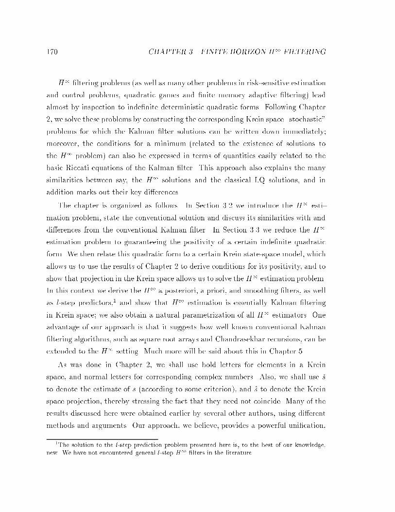
��� CHAPTER �� FINITE HORIZON H� FILTERING
H� �ltering problems �as well as many other problems in risk�sensitive estimation
and control problems� quadratic games and �nite memory adaptive �ltering� lead
almost by inspection to inde�nite deterministic quadratic forms� Following Chapter
� we solve these problems by constructing the corresponding Krein space �stochastic�
problems for which the Kalman �lter solutions can be written down immediately�
moreover� the conditions for a minimum �related to the existence of solutions to
the H� problem� can also be expressed in terms of quantities easily related to the
basic Riccati equations of the Kalman �lter� This approach also explains the many
similarities between say� the H� solutions and the classical LQ solutions� and in
addition marks out their key di�erences�
The chapter is organized as follows� In Section �� we introduce the H� esti�
mation problem� state the conventional solution and discuss its similarities with and
di�erences from the conventional Kalman �lter� In Section ��� we reduce the H�
estimation problem to guaranteeing the positivity of a certain inde�nite quadratic
form� We then relate this quadratic form to a certain Krein state�space model� which
allows us to use the results of Chapter to derive conditions for its positivity� and to
show that projection in the Krein space allows us to solve theH� estimation problem�
In this context we derive the H� a posteriori� a priori� and smoothing �lters� as well
as l�step predictors�� and show that H� estimation is essentially Kalman �ltering
in Krein space� we also obtain a natural parametrization of all H� estimators� One
advantage of our approach is that it suggests how well known conventional Kalman
�ltering algorithms� such as square root arrays and Chandrasekhar recursions� can be
extended to the H� setting� Much more will be said about this in Chapter ��
As was done in Chapter � we shall use bold letters for elements in a Krein
space� and normal letters for corresponding complex numbers� Also� we shall use �s
to denote the estimate of s �according to some criterion�� and �s to denote the Krein
space projection� thereby stressing the fact that they need not coincide� Many of the
results discussed here were obtained earlier by several other authors� using di�erent
methods and arguments� Our approach� we believe� provides a powerful uni�cation�
�The solution to the l�step prediction problem presented here is� to the best of our knowledge�new� We have not encountered general l�step H� �lters in the literature�

���� H� ESTIMATION ���
with immediate insights to various extensions�
��� H� Estimation
Several H���ltering algorithms have been recently derived by a variety of methods
in both the continuous and discrete�time cases �see� e�g�� �Kwa �� DGKF �� KN���
Bas��� LS��� ST�� YS��� Gri��� and the references therein��
Many authors have noticed some formal similarities between the H� �lters and
the conventional Kalman �lter� however we shall further clarify this connection by
showing that H� �lters are nothing more than certain Krein space Kalman �lters� In
other words� theH� �lters can be viewed as recursively performing a �Gram�Schmidt�
orthogonalization �or projection� procedure on a convenient set of observation data
that obey a state�space model whose state evolves in an inde�nite metric space� This
is of signi�cance since it yields a geometric derivation of theH� �lters� and because it
uni�es H� and H� estimation in a simple framework� Moreover� once this connection
has been made explicit� many known alternative and more e�cient algorithms� such
as square�root arrays and Chandrasekhar equations�HSK�c�� can be applied to the
H��setting as well� Also our results deal directly with the time�varying scenario�
Finally� we note that although we restrict ourselves here� to the discrete�time case�
however� the continuous time analogs follow the same principles�
����� Formulation of the H� Filtering Problem
Consider a time�variant state�space model of the form
��� xi�� � Fixi �Giui� x�
yi � Hixi � vi� i � �������
where Fi � Cn�n� Gi � Cn�m and Hi � Cp�n are known matrices� x�� fuig� and fvig are
unknown quantities and yi is the measured output� We can regard vi as a measurement
noise and ui as a process noise or driving disturbance� We make no assumption on the
nature of the disturbances �e�g� � normally distributed� uncorrelated� etc�� In general�

�� CHAPTER �� FINITE HORIZON H� FILTERING
we would like to estimate some arbitrary linear combination of the states� say
si � Lixi�
where Li � Cq�n is given� using the observations fyjg� Let �siji � Ff�y�� y�� � � � � yi�
denote the estimate of si given observations fyjg from time � up to and including
time i� and �si � Fp�y�� y�� � � � � yi��� denote the estimate of si given observations fyjg
from time � to time i � �� We then have the following two estimation errors� the
�ltered error
ef�i � �siji � Lixi� �����
and the predicted error
ep�i � �si � Lixi� ������
�
�
�
�
�
�
�
� � f�zj � Ljxjgij��
f�zjjj � Ljxjgij��
Ti�Fp�
Ti�Ff �fujgij��
fvjgij��
fujgij��
������ �x� � �x��
fvjgij��
������ �x� � �x��
Figure ���� Transfer matrix from disturbances to �ltered and predicted estimationerrors�
As depicted in Fig� ���� let Ti�Ff� and Ti�Fp� denote the transfer operators that
map the unknown disturbances f������ �x� � �x��� fujg
ij��� fvjg
ij��g �where �x� denotes
an initial guess for x�� and �� is a given positive de�nite matrix� to the �ltered and

���� H� ESTIMATION ���
predicted errors fef�jgij�� and fep�jgij��� respectively� The problem is to choose the
functionals Ff��� and Fp��� so as to respectivelyminimize theH� norm of the transfer
operators Ti�Ff � and Ti�Fp��
De�nition ����� The H� norm of a transfer operator T is de�ned as
kTk� � supu�h� �u ���
kTuk�kuk�
where kuk� is the h��norm of the causal sequence fukg� i�e� kuk�� �
P�k��u
�kuk�
The H� norm thus has the interpretation of being the maximum energy gain from
the input u to the output y� Our problem may now be formally stated as follows�
Problem ����� �Optimal H� Problem� Find �ltered and predicted H��optimal
estimation strategies �siji � Ff �y�� y�� � � � � yi� and �si � Fp�y�� y�� � � � � yi��� that respec�
tively minimize k Ti�Ff� k� and k Ti�Fp� k�� and obtain the resulting
��f�o � infFfk Ti�Ff � k��
� infFfsupx��u�h��v�h�
Pi
j��e�f�j
ef�j
�x���x�������x���x���
Pi
j��u�juj�
Pi
j��v�jvj
�����
and
��p�o � infFp k Ti�Fp� k��
� infFp supx��u�h��v�h�
Pi
j��e�p�j
ep�j
�x���x�������x���x���
Pi��
j��u�juj�
Pi��
j��v�jvj
������
where �� is a positive de�nite matrix that re�ects a priori knowledge as to how close
x� is to the initial guess �x��
Note that the in�mum in ������ is taken over all strictly causal estimators Fp�
whereas in ����� the estimators Ff are only causal� since they have additional access
to yi� This is relevant since the solution to the H� problem� as we shall see� depends
on the structure of the information available to the estimator�
The above problem formulation shows that H� optimal estimators guarantee the
smallest estimation error energy over all possible disturbances of �xed energy� They
�� CHAPTER �� FINITE HORIZON H� FILTERING
are therefore conservative �and at times over�conservative�� which results in a better
robust behaviour to disturbance variation�
A closed form solution to the optimal H� estimation problem is available only in
some special cases �see e�g� � �HSK��a� and Chapter ��� and so it is common in the
literature to settle for a suboptimal solution�
Problem ����� �Suboptimal H� Problem� Given scalars �f � � and �p � ��
H� suboptimal estimation strategies �siji � Ff �y�� y�� � � � � yi� �known as an a posteriori
�lter� and �si � Fp�y�� y�� � � � � yi��� �known as an a priori �lter� that respectively
achieve k Ti�Ff� k�� �f and k Ti�Fp� k�� �p� In other words� �nd strategies that
respectively achieve
supx��u�h� �v�h�
Pij�� e
�f�jef�j
�x� � �x��������x� � �x�� �
Pij�� u
�juj �
Pij�� v
�jvj
� ��f ������
and
supx��u�h��v�h�
Pij�� e
�p�jep�j
�x� � �x��������x� � �x�� �
Pi��j�� u
�juj �
Pi��j�� v
�jvj
� ��p � ������
This clearly requires checking whether �f � �f�o and �p � �p�o�
Note that the solutions to Problem ���� can be obtained to desired accuracy by
iterating on the �f and �p of Problem ���� From here on we shall be only dealing
with Problem ����
Note that since the upper limits in the aforementioned sums are the �nite number
i� the problems de�ned above are �nite�horizon problems� So�called in�nite�horizon
problems can be considered if we de�ne T �Ff� and T �Fp� as the transfer operators
that map fx�� �x�� fujg�j��� fvjg�j��g to fef�jg
�j�� and fep�jg
�j��� respectively� Then by
guaranteeing k Ti�Ff� k�� �f and k Ti�Fp� k�� �p for all i� we can solve the in�nite�
horizon problems k T �Ff� k�� �f and k T �Fp� k�� �p� respectively� However� as we
have seen in Sec� ����� direct solutions are also possible� We shall study the in�nite
horizon problem in more detail in Chapter ��
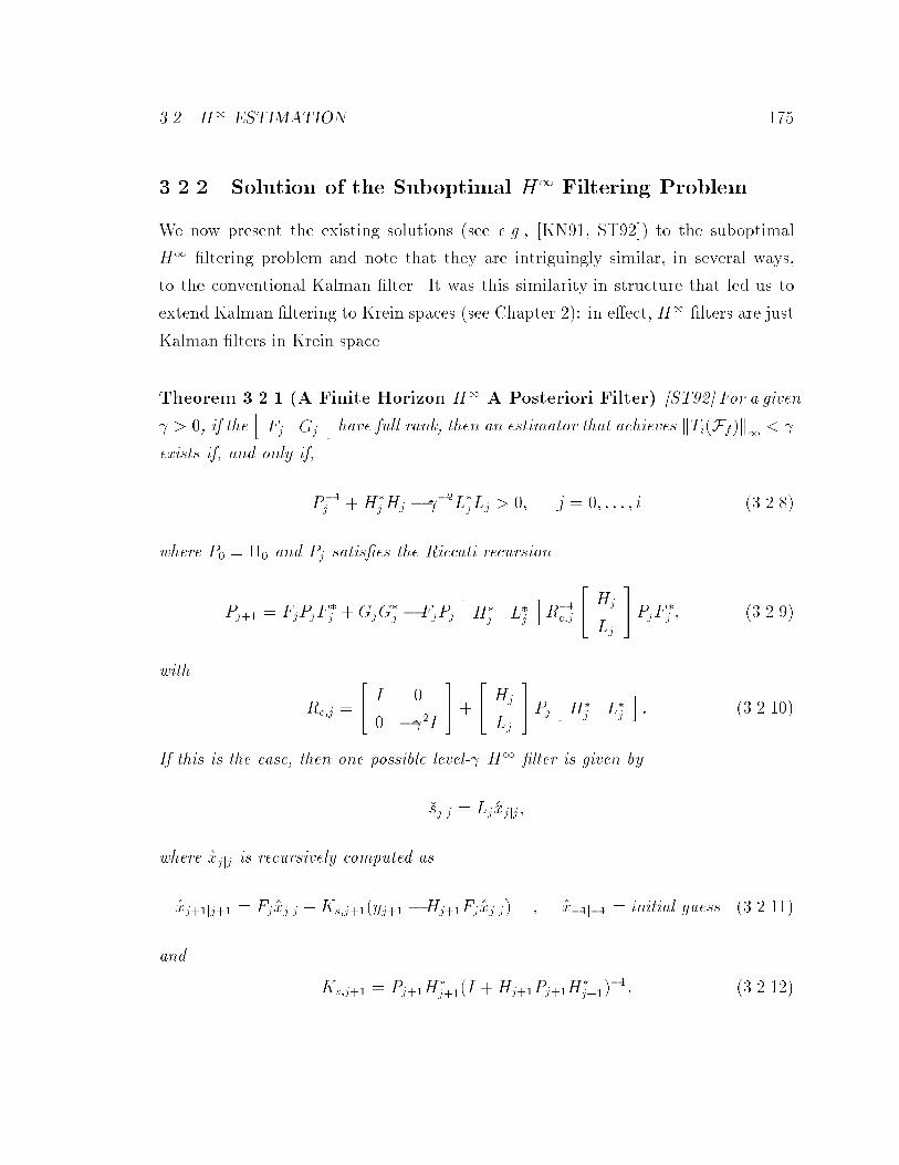
���� H� ESTIMATION ���
����� Solution of the Suboptimal H� Filtering Problem
We now present the existing solutions �see e�g�� �KN��� ST��� to the suboptimal
H� �ltering problem and note that they are intriguingly similar� in several ways�
to the conventional Kalman �lter� It was this similarity in structure that led us to
extend Kalman �ltering to Krein spaces �see Chapter �� in e�ect� H� �lters are just
Kalman �lters in Krein space�
Theorem ����� �A Finite Horizon H� A Posteriori Filter� ST�� For a given
� � �� if thehFj Gj
ihave full rank� then an estimator that achieves kTi�Ff�k� � �
exists if� and only if�
P��j �H�
jHj � ���L�jLj � �� j � �� � � � � i ���� �
where P� � �� and Pj satis�es the Riccati recursion
Pj�� � FjPjF�j �GjG
�j � FjPj
hH�
j L�j
iR��
e�j
�� Hj
Lj
��PjF
�j � ������
with
Re�j �
�� I �
� ���I
���
�� Hj
Lj
��Pj
hH�
j L�j
i� �������
If this is the case� then one possible level�� H� �lter is given by
�sjjj � Lj�xjjj�
where �xjjj is recursively computed as
�xj��jj�� � Fj�xjjj �Ks�j���yj�� �Hj��Fj�xjjj� � �x��j�� � initial guess �������
and
Ks�j�� � Pj��H�j���I �Hj��Pj��H
�j���
��� ������
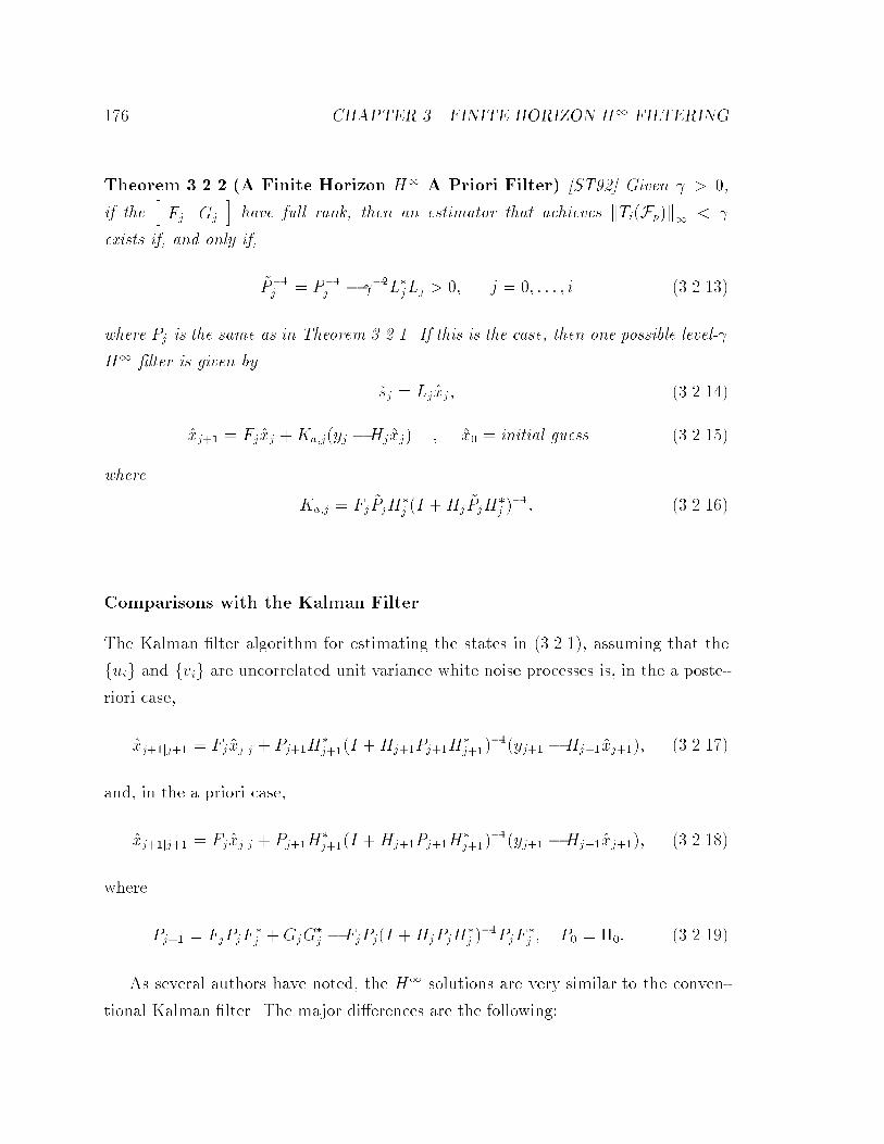
��� CHAPTER �� FINITE HORIZON H� FILTERING
Theorem ����� �A Finite Horizon H� A Priori Filter� ST�� Given � � ��
if thehFj Gj
ihave full rank� then an estimator that achieves kTi�Fp�k� � �
exists if� and only if�
�P��j � P��
j � ���L�jLj � �� j � �� � � � � i �������
where Pj is the same as in Theorem ����� If this is the case� then one possible level��
H� �lter is given by
�sj � Lj�xj� ������
�xj�� � Fj�xj �Ka�j�yj �Hj�xj� � �x� � initial guess �������
where
Ka�j � Fj�PjH
�j �I �Hj
�PjH�j ���� �������
Comparisons with the Kalman Filter
The Kalman �lter algorithm for estimating the states in ������� assuming that the
fuig and fvig are uncorrelated unit variance white noise processes is� in the a poste�
riori case�
�xj��jj�� � Fj�xjjj � Pj��H�j���I �Hj��Pj��H
�j���
���yj�� �Hj���xj���� �������
and� in the a priori case�
�xj��jj�� � Fj�xjjj � Pj��H�j���I �Hj��Pj��H
�j���
���yj�� �Hj���xj���� ����� �
where
Pj�� � FjPjF�j �GjG
�j � FjPj�I �HjPjH
�j ���PjF
�j � P� � ��� �������
As several authors have noted� the H� solutions are very similar to the conven�
tional Kalman �lter� The major di�erences are the following�

���� H� ESTIMATION ���
� The structure of the H� estimators depends� via the Riccati recursion �������
on the linear combination of the states that we intend to estimate �i�e� the Li��
This is as opposed to the Kalman �lter� where the estimate of any linear com�
bination of the state is given by that linear combination of the state estimate�
Intuitively� this means that the H� �lters are speci�cally tuned towards the
linear combination Lixi�
� We have additional conditions� ���� � or �������� that must be satis�ed for the
�lter to exist� in the Kalman �lter problem the Li would not appear� and the
Pi would be positive de�nite� so that ���� � and ������� would be immediate�
� We have inde�nite �covariance� matrices� e�g� �
�� I
���I
�� vs� just I in the
Kalman �lter�
� As � ��� the Riccati recursion ������ reduces to the Kalman �lter recursion
�������� �This suggests that the H� norm of the conventional Kalman �lter
may be quite large� and that it may have poor robustness properties�� Note
also that condition ������� is more stringent than condition ���� �� indicating
that the existence of an a priori �lter of level � implies the existence of an a
posteriori �lter of the same level� but not necessarily vice versa��
Despite these di�erences� we shall show by applying the results of Chapter � that
the �lters of Theorems ���� and ��� can in fact be obtained as certain Kalman �lters�
not in an H� �Hilbert� space� but in a certain inde�nite vector space� called a Krein
space� The inde�nite covariances and the appearance of Li in the Riccati equation
will be easily explained in this framework� The additional condition ���� � will be
seen to arise from the fact that in Krein space� unlike as in the usual Hilbert space
context� quadratic forms need not always have minima or maxima� unless certain
additional conditions are met� Moreover� our approach will provide a simpler and
more general alternative to the tests ���� � and ��������
�We shall have more to say about this in Chapter ���

�� CHAPTER �� FINITE HORIZON H� FILTERING
��� Derivation of the H� Filters
In Sec� ���� we derived the H� suboptimal �lters using the canonical factoriza�
tion of a certain inde�nite transfer operator� Here we can take the same approach�
the inde�nite transfer operator will now be a �nite inde�nite matrix �or Gramian�
and the canonical factorization will correspond to a �block� LDU �lower�diagonal�
factorization�� As we have seen in Chapter � when the Gramian has state�space
structure �as it does in the H� state�space estimation problem under consideration�
the triangular factorization can be obtained from the Krein space Kalman �lter� This
route will then lead us both to the solution of theH� �ltering problems �via the Krein
space Kalman �lter� which incidentally also explains the connections with the con�
ventional Kalman �lter� and to the existence conditions for such �lters �since an LDU
factorization with certain inertia properties requires additional conditions�� However�
we shall here take a slightly di�erent �and closer to the general spirit of Chapter �
route to the solution� i�e�� one that is based upon associating an inde�nite quadratic
form �instead of an inde�nite transfer operator� with the H� �ltering problem� There
are� of course� close connections between these two approaches and we shall comment
on them wherever deemed appropriate�
As shown Chapter � the �rst step is to associate an inde�nite quadratic form
with each of the �level �� a posteriori and a priori �ltering problems� This will lead
us to construct an appropriate �so�called partially equivalent� Krein space state�space
model� the Kalman �lter for which will allow us to compute the stationary points for
the H� quadratic forms� conditions that these are actually minima will be deduced
from the general results of Chapter � and shown to be just ���� � and ��������
simpler equivalent conditions will also be noted�
Therefore we begin by examining the structure of the H� problem in more detail�
The goal will be to relate the problem to an inde�nite quadratic form� We shall �rst
consider the a posteriori �ltering problem�

���� DERIVATION OF THE H� FILTERS ���
����� The Suboptimal H� Problem and Quadratic Forms
Referring to Problem ���� we �rst note that kTi�Ff�k� � �f � implies that for all
nonzero fx�� fujgij��� fvjgij��g
Pij�� j�sjjj � Ljxjj�
�x� � �x������� �x� � �x�� �
Pij�� jujj
� �Pi
j�� jyj �Hjxjj�� ��f � �������
Moreover� ������� implies that for all k � i� we must have
Pkj�� j�sjjj � Ljxjj�
�x� � �x������� �x� � �x�� �
Pkj�� jujj
� �Pk
j�� jyk �Hixij�� ��f � ������
We remark that if the fyjgij�� are all zero then it is easy to see that the f�sjjjg must
all be zero as well� Therefore we need only consider the case where fyjgij�� is a
nonzero sequence� We shall then prove the following result� relating the condition
kTi�Ff�k� � �f to the positivity of a certain inde�nite quadratic form� Incidentally
from now on� without loss of generality� we assume �x� � �� a nonzero �x� � � will only
change the initial condition of the �lter�
Lemma ����� �Inde�nite Quadratic Form� Given �f � �� then kTi�Ff�k� � �f
if� and only if� there exists �skjk � Ff�y�� � � � � yk� �for all � � k � i� such that for
all complex vectors x�� for all causal sequences fujgij�� and for all nonzero causal
sequences fyjgij��� the scalar quadratic form
Jf�k�x�� u�� � � � � uk� y�� � � � � yk� � x������ x� �
Pkj�� u
�juj�Pk
j���yj �Hjxj���yj �Hjxj�� ���f
Pkj����sjjj � Ljxj����sjjj � Ljxj�
�������
satis�es
Jf�k�x�� u�� � � � � uk� y�� � � � � yk� � � for all � � k � i� ������
Proof� For one direction� assume there exists a solution �skjk �for all k � i� that
achieves kTi�Ff �k� � �f � Then if we multiply both sides of ������ by the positive
denominator on the LHS� we obtain �������

� � CHAPTER �� FINITE HORIZON H� FILTERING
Conversely� if there exists a solution �skjk �for all k � i� that achieves ������� we
can divide both sides of ������ by the positive quantity
x������ x� �
kXj��
u�juj �kX
j��
�yj �Hjxj���yj �Hjxj�
to obtain ������� and thereby kTi�Ff�k� � �f �
Remark� Lemma ����� is a straightforward restatement of the inequality ������
which is required of all suboptimal H� a posteriori �lters with level �f � However�
the statement of Lemma ����� given below� is a key result� since it shows how to
check the conditions of Lemma ����� by computing the stationary point of the in�
de�nite quadratic form Jf�k�x�� u�� � � � � uk� y�� � � � � yk� and checking its condition for a
minimum� This is in the spirit of the approach taken in Chapter �
Note that since the �skjk are functions of the fyjgkj��� Jf�k�x�� u�� � � � � uk� y�� � � � � yk�
is really a function of only fx�� u�� � � � � uk� y�� � � � � ykg� Moreover� since the fyjg are
�xed observations� the only free variables in Jf�k�x�� u�� � � � � uk� y�� � � � � yk� are the
disturbances fx�� u�� � � � � ukg� We then have the following result�
Lemma ����� �Positivity Condition� The scalar quadratic forms
Jf�k�x�� u�� � � � � uk� y�� � � � � yk��
satisfy the conditions � � ���� if� and only if� for all � � k � i�
�i� Jf�k�x�� u�� � � � � uk� y�� � � � � yk� has a minimum with respect to fx�� u�� u�� ���ukg�
�ii� The f�skjkgik�� can be chosen such that the value of Jf�k�x�� u�� � � � � uk� y�� � � � � yk�
at this minimum is positive� viz��
minfx��u������ukg
Jf�k�x�� u�� � � � � uk� y�� � � � � yk� �s�j�� � � � � �skjk� � ��
Proof� Assume Jf�k�x�� fujgkj��� fyjgkj��� � �� then condition �i� is clearly satis�ed
because if Jf�k�x�� fujgkj��� fyjgkj��� does not have a minimum over fx�� u�� � � � � ukg�

���� DERIVATION OF THE H� FILTERS � �
then it is always possible to choose fx�� fujgkj��g so as to make Jf�k�x�� fujgkj��� fyjgkj���
arbitrarily small and negative� Moreover� the existence of a minimum� along with
Jf�k�x�� fujgkj��� fyjgkj��� � �� guarantees condition �ii� since the value at the mini�
mum must be positive�
Conversely� if �i� and �ii� hold� then it follows that Jf�k�x�� fujgkj��� fyjgkj��� � ��
����� A Krein Space State�Space Model
To apply the methodology of Chapter � we �rst identify the inde�nite quadratic form
Jf�k as a special case of the general form studied in Theorem ��� by rewriting it as
Jf�k�x�� u�� � � � � uk� y�� � � � � yk� �
x������ x��
kXj��
u�juj�kX
j��
��� yj
�sjjj
���
�� Hj
Lj
��xj
A� �� I �
� ����f I
����� yj
�sjjj
���
�� Hj
Lj
��xj
A �
�������
Then by Lemmas ���� and ���� we can introduce the following Krein space
state�space model� ���������
xj�� � Fjxj �Gjuj�� yj
�sjjj
�� �
�� Hj
Lj
��xj � vj
�������
with
h
�����x�
uj
vj
� � ������x�
uk
vk
� �i �
��������
�� � �
� I�jk �
� �
�� I �
� ���fI
�� �jk
� �
�������
Note that Qj � I� Sj � �� �� � �� and that we must consider a Krein space since
Rj �
�� I
���fI
�� ����� �
is inde�nite�
�We should also mention that the output Gramian of
�yj
�sjjj
�in the state�space model ����
��� is simply the inde�nite Gramian of Theorem ����� whose canonical factorization is needed in

� CHAPTER �� FINITE HORIZON H� FILTERING
����� Proof of Theorem �����
In order to focus the discussion we brie y review the procedure of the proof�
� Referring to Lemma ����� we �rst need to check the whether Jf�k�x�� fuj� yjgkj���
has a minimum with respect to fx�� fujgkj��g� This is done via the Krein space
Kalman �lter corresponding to �������������� and yields the condition ���� �
along with several equivalent conditions�
� Next we need to choose the f�skjkgik�� such that the value of Jf�k�x�� fuj� yjgkj���
is positive at its minimum� Now according to Theorem ���� the value at
the minimum is Jf�k�min� �Pk
j�� ejR��e�j ej� where ej is the innovations corre�
sponding to �������������� We can then compute the fejg using the Krein space
Kalman �lter� and thereby choose the appropriate f�skjkgik�� which yields the
desired a posteriori �lter�
A remark on the strong regularity of the model ���������� �� In what follows
we would like to use the Krein space Kalman �lter corresponding to the state�space
model �������������� This of course requires the strong regularity of its output Gramian
matrix� which we denote by Rys�since the output of ������� consists of both a y and
a s component��
If Rysis strongly regular� then the Krein space Kalman �lter may be applied to
check for the positivity of Jf�k for each � � k � i� But what if Rysis not strongly
regular! Then it turns out that Jf�k cannot be positive for all � � k � i� To see why
suppose that Jf�k � � for some arbitrary k� Then Jf�k must have a minimum� and
according to Lemma ���� the leading kk block submatrices of Rysand R�S�QS �
R must have the same inertia� Now due to ����� �� all leading submatrices of R are
nonsingular� and since k was arbitrary� the same will be true of Rys� Therefore Ry
swill
be strongly regular�
To summarize� we may use the Krein space Kalman �lter to check the positivity
of Jf�k� If one of the Re�k becomes singular �so that Rysis no longer strongly regular��
the solution of the H� estimation problem� Since the Krein space Kalman �lter corresponding to��� can be used to perform this canonical factorization� we will shortly albeit via di�erent route see that it plays a crucial role in the solution�

���� DERIVATION OF THE H� FILTERS � �
Jf�k will lose its positivity by default��
Proof of existence condition ��������
The Riccati recursion corresponding to ������� is the exact same Riccati recursion
that was given by ������ in Theorem ����� We can now apply any of the condi�
tions for a minimum developed in Chapter � to check whether a minimum exists for
Jf�k�x�� u�� � � � � uk� y�� � � � � yk� for all � � k � i� If we assume that thehFk Gk
ihave
full rank� then according to Lemma ���� Jf�k�x�� u�� � � � � uk� y�� � � � � yk� will have a
minimum for all � � k � i� if� and only if�
P��jjj � P��
j �hH�
j L�j
i �� I
���fI
���� �� Hj
Lj
�� � �
which yields the condition ���� ��
Since we still need to satisfy the second condition of Lemma ����� this� of course�
only shows that ���� � is a necessary condition for the existence of an H� a posteriori
�lter of level �f � However� we shall later show that if the minimum condition is
satis�ed then the second condition of Lemma ���� can also be satis�ed� Therefore
���� � is indeed necessary and su�cient for the existence of the �lter�
Other Existence Conditions
Using the results Chapter � we can obtain alternative conditions for the existence
of H� a posteriori �lters of level �f � If we use Lemma ����� we have the following
condition�
�Another way to show the strong regularity of Ry
sis to appeal to Theorem ������ There it was
shown in a more general setting that an H� �lter exists if� and only if� Ry
sadmits a canonical
factorization with a certain prescribed inertia� It is easy to check that the existence of this canonicalfactorization requires� at the very least� the strong regularity of Ry
s�

� CHAPTER �� FINITE HORIZON H� FILTERING
Lemma ����� �Alternative Test for Existence� The condition � ����� can be re�
placed by the condition that
Rj �
�� I
���fI
�� and Re�j �
�� I
���fI
���
�� Hj
Lj
��Pj
hH�
j L�j
i
have the same inertia for all � � j � i� We no longer require thathFj Gj
ihave
full rank� and the size of the matrices involved is generally smaller than in � ������
Using a block triangular factorization of Re�j� and the fact that when we have a
minimum� Pj is positive de�nite� we can show the following result�
Corollary ����� �Alternative Test for Existence� The condition of Lemma � �
is equivalent to
I �HjPjH�j � � and � ��fI � Lj�P
��j �H�
jHj���L�j � �� �������
for all � � j � i�
The test of Lemma ����� has various advantages over ���� � that are mentioned in
the discussions following Lemma ���� In particular� Lemma ����� allows us to go to
a square�root form of the H� �ltering algorithm� where there is no need to explicitly
check for the existence condition � these conditions are built into the the square�root
recursions themselves� so that a solution exists if� and only if� the algorithm can be
performed �see �HSK�c� and Chapter ���
Many alternative existence conditions can also be obtained� Here is one that
follows Lemma �����
Lemma ����� �Alternative Test for Existence� If the fFjg are nonsingular� an
H� a posteriori �lter of level �f exists� if� and only if�
Pi�� � ��
and
I �G�jP
��j��Gj � � j � �� �� � � � � i�

���� DERIVATION OF THE H� FILTERS � �
Construction of the H� a posteriori �lters
To complete the proof of Theorem ���� we still need to show that if a minimum over
fx�� u�� � � � � ukg exists for all � � k � i� then we can �nd the estimates f�skjkgik�� such
that the value of Jf�k�x�� u�� � � � � uk� y�� � � � � yk� at its minimum is positive�
According to Theorem ���� the minimum value of Jf�k�x�� u�� � � � � uk� y�� � � � � yk�
iskX
j��
he�y�j e�s�j
iR��
e�j
�� ey�j
es�j
�� �
kXj��
�� yj � �yjjj��
�sjjj � �sjjj��
��� �� I �HjPjH
�j HjPjL
�j
LjPjH�j ���fI � LjPjL
�j
���� �� yj � �yjjj��
�sjjj � �sjjj��
��
where �yjjj�� and �sjjj�� are obtained from the Krein space projections of yj and �sjjj
onto Lnfylg
j��l�� � f�sljlg
j��l��
o� respectively� Thus �sjjj�� is a linear function of fylg
j��l�� �
Using the block triangular factorization of the Re�j we may rewrite the above as
kXj��
�� yj � �yjjj��
�sjjj � �sjjj
��� �� I �HjPjH
�j �
� ���fI � Lj�P��j �H�
jHj���L�j
���� �� yj � �yjjj��
�sjjj � �sjjj
��
where�� yj � �yjjj��
�sjjj � �sjjj
�� ��
�� I �
�LjPjH�j �I �HjPjH
�j ��� I
���� yj � �yjjj��
�sjjj � �sjjj��
�� � ��������
Or in other words�
�sjjj � �sjjj�� � LjPjH�j �I �HjPjH
�j ����yj � �yjjj���� ��������
Note that �sjjj is obtained from the Krein space projection of �sjjj onto Lnfylg
jl��� f�sljlg
j��l��
o�
and is therefore a linear function of fylgjl��� Recall from Corollary ����� that
I �HjPjH�j � � and � ��fI � Lj�P
��j �H�
jHj���L�j � �� �������
Therefore all we must do is choose some �sjjj such that
Pkj���yj � �yjjj���
��I �HjPjH�j ����yj � �yjjj��� ��������
�Pk
j����sjjj � �sjjj������fI � Lj�P
��j �HjH
�j ���L�j
�����sjjj � �sjjj� � ��
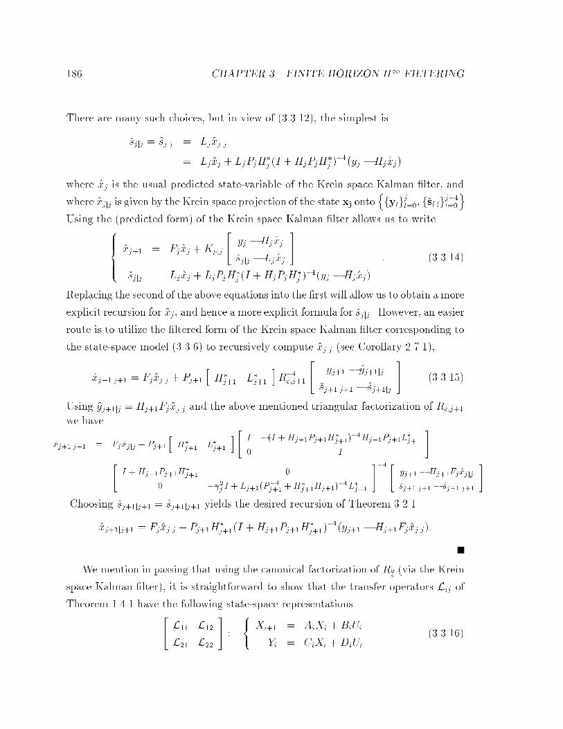
� � CHAPTER �� FINITE HORIZON H� FILTERING
There are many such choices� but in view of �������� the simplest is
�sjjj � �sjjj � Lj�xjjj
� Lj�xj � LjPjH�j �I �HjPjH
�j ����yj �Hj �xj�
where �xj is the usual predicted state�variable of the Krein space Kalman �lter� and
where �xjjj is given by the Krein space projection of the state xj ontonfylg
jl��� f�sljlg
j��l��
o�
Using the �predicted form� of the Krein space Kalman �lter allows us to write���������
�xj�� � Fj�xj �Kp�j
�� yj �Hj �xj
�sjjj � Lj �xj
��
�sjjj � Lj �xj � LjPjH�j �I �HjPjH
�j ����yj �Hj�xj�
� �������
Replacing the second of the above equations into the �rst will allow us to obtain a more
explicit recursion for �xj� and hence a more explicit formula for �sjjj � However� an easier
route is to utilize the �ltered form of the Krein space Kalman �lter corresponding to
the state�space model ������� to recursively compute �xjjj �see Corollary ������
�xj��jj�� � Fj�xjjj � Pj��
hH�
j�� L�j��
iR��
e�j��
�� yj�� � �yj��jj
�sj��jj�� � �sj��jj
�� ��������
Using �yj��jj � Hj��Fj�xjjj and the above mentioned triangular factorization of Re�j��
we have
�xj��jj�� � Fj�xjjj � Pj��
hH�
j�� L�j��
i� I �I �Hj��Pj��H�j��
��Hj��Pj��L�j��
� I
��
I �Hj��Pj��H�j�� �
� ���f I � Lj��P��j�� �H�
j��Hj�� ��L�j��
��� �yj�� �Hj��Fj�xjjj
�sj��jj�� � �sj��jj��
�
Choosing �sj��jj�� � �sj��jj�� yields the desired recursion of Theorem ����
�xj��jj�� � Fj�xjjj � Pj��H�j���I �Hj��Pj��H
�j���
���yj�� �Hj��Fj�xjjj��
We mention in passing that using the canonical factorization of Rys�via the Krein
space Kalman �lter�� it is straightforward to show that the transfer operators Lij of
Theorem ���� have the following state�space representations�� L�� L��
L�� L��
�� �
��� Xi�� � AiXi �BiUi
Yi � CiXi �DiUi
��������

���� DERIVATION OF THE H� FILTERS � �
where�����������������������������������
Ai � Fi
Gi � Kp�i
�� �Ip �HiPiH
�i �
��� �
�LiPiH�i �Ip �HiPiH
�i ����� ���Iq � LiPi�I �H�
i HiPi���L�����
��
Ci �
�� Hi
�Li
��
Di �
�� Ip �
� Iq
��
�
��������
Using the above state�space representation� it is straightforward to show �though we
shall not provide the algebraic manipulations here� that the central �lter� Kcen �
�L��L���� � has state�space model given by the recursions of Theorem ����� It is also
possible to use the Lij �obtained above� to parametrize all possible H� �lters of level
� along the lines of Theorem ����� Here� however� we shall take a di�erent route to
this parametrization which has the bene�t of allowing for nonlinear estimators�
����� Parametrization of All H� A Posteriori Filters
The �lter of Theorem ���� is one among many possible �lters with level �� All
�lters that guarantee Jf�k�x�� u�� � � � � uk� y�� � � � � yk� � � are represented by �������
and ��������� It is useful to formalize this representation in the following result�
Lemma ����� �All H� A Posteriori Estimators� All H� a posteriori estima�
tors that achieve a level �f �assuming they exist� are given by any �sjjj � Ff�j�y�� � � � yj�
that satisfy
kXj��
�� yj �Hj �xj
�sjjj � Lj �xj
���
R��e�j
�� yj �Hj �xj
�sjjj � Lj�xj
�� � �� � � k � i ������ �
where �xj satis�es the recursion�
�xj�� � Fj�xj �Kp�j
�� yj �Hj�xj
�sjjj � Lj�xj
�� � �x� ��������

� CHAPTER �� FINITE HORIZON H� FILTERING
with
Kp�j � FjPj
hH�
j L�j
iR��
e�j and Re�j �
�� Ip �
� ���fIq
���
�� Hj
Lj
��Pj
hH�
j L�j
i�������
and
Pj�� � FjPjF�j �GjQjG
�j �Kp�jRe�jK
�p�j� P� � ��� �������
We may also use these expressions to obtain a more explicit characterization of
all possible estimators� Similar results appear in �KN��� ST�� GL����
Theorem ����� �All H� A Posteriori Estimators� All H� a posteriori estima�
tors that achieve a level �f �assuming they exist� are given by
�sjjj � Lj �xjjj � ���fI � Lj�P��j �H�
jHj���L�j �
�
� ������
Sj
��I �HjPjH
�j �
�
� �yj �Hj �xjjj�� � � � � �I �H�P�H�� �
�
� �y� �H��x�j���
where �xjjj satis�es the recursion
�xj��jj�� � Fj�xjjj �Ks�j���yj�� �Hj��Fj�xjjj��Kc�j��sjjj � Lj�xjjj� �������
with Ks�j�� the same as in Theorem �����
Kc�j � �I � Pj��Hj��H�j���
��Fj�P��j �HjH
�j � ���f LjL
�j ���L�j � ������
and
S�aj� � � � � a�� �
���������
S��a��
S��a�� a�����
Sj�aj� � � � � a��
� �
is any �possibly nonlinear� contractive causal mapping� i�e��
kXj��
jSj�aj� � � � � a��j� �
kXj��
jajj� for all k � �� �� � � � � i�

���� DERIVATION OF THE H� FILTERS � �
Remark� Note that when the contraction of Theorem ����� is chosen as S � �� then
we have �sjjj � Lj �xjjj� and ������� reduces to the recursion of Theorem �����
Proof of Theorem ������ Expression �������� may be rewritten as�
Pkj���yj �Hj�xj���I �HjPjH
�j ����yj �Hj�xj� �������
�Pk
j����sjjj � L�xjjj������fI � Lj�P
��j �HjH
�j ���L�j
�����sjjj � Lj �xjjj� � �
where �xj and �xjjj denote the Krein space projections of xj ontonfylg
j��l�� � f�sljlg
j��l��
oand
nfylg
jl��� f�sljlg
j��l��
o� respectively� Therefore �xj and �xjjj are related through one
additional projection onto yj� and we may write
�xjjj � �xj � PjH�j �I �HjPjH
�j ����yj �Hj �xj�� �������
Therefore
yj �Hj �xjjj ��I �HjPjH
�j �I �HjPjH
�j �����yj �Hj �xj�
� �I �HjPjH�j ����yj �Hj�xj�
so that
�yj �Hj �xj� � �I �HjPjH�j ��yj �Hj �xjjj��
Now ������� can be written as�
Pkj���yj �Hj �xjjj�
��I �HjPjH�j ��yj �Hj �xjjj�
�Pk
j����sjjj � Lj�xjjj������fI � Lj�P
��j �HjH
�j ���L�j
�����sjjj � Lj �xjjj� � �
or equivalently�
k ���fI�Lj�P��j �HjH
�j ���L�j �
� �
� ��sjjj� �sjjj� k�� � k �I�HjPjH
�j �
�
� �yj�Hj�xjjj� k�� �
Since �sjjj is a causal function of the observations yj� then ��sjjj � �sjjj� will also be a
causal function of �yj �Hj �xjjj�� Therefore using the above expression� we can write
��������fI � L��P
��� �H�H
�� ���L���
� �
� ��s�j� � �s�j�����
���fI � Li�P��i �HiH
�i ���L�i �
� �
� ��siji � �siji�
� � � S
������I �H�P�H
�� �
�
� �y� �H��x�j�����
�I �HiPiH�i �
�
� �yi �Hi�xiji�
� �

��� CHAPTER �� FINITE HORIZON H� FILTERING
for some causal contractive mapping S� Eq� ������ now readily follows�
Finally� we must show �������� To this end� recall from the proof of Theorem
���� �see ��������� that the recursion for �xj is given by
�xj��jj�� � Fj�xjjj � Pj��
hH�
j�� L�j��
iR��
e�j��
�� yj�� � �yj��jj
�sj��jj�� � �sj��jj
�� �
Using ������� to replace �xj by �xjjj yields� after some algebra� the desired recursion
��������
Note that although the �lter obtained in Theorem ���� is linear� the full para�
metrization of all H� �lters with level �f is given by a nonlinear causal contractive
mapping S� The �lter of Theorem ���� is known as the central �lter and as we
have seen� corresponds to S � �� This central �lter has a number of other interesting
properties� It corresponds� as we shall see in the next chapter� to the risk�sensitive op�
timal �lter �Whi���� and� as we have seen in Chapter �� to the maximum entropy �lter
�GM ��� Moreover� in the game theoretic formulation of the H� problem� the central
�lter corresponds to the solution of the game �BB���� In our context� the central
�lter is recognized as the Krein space Kalman �lter corresponding to the state�space
model ��������
����� Derivation of the A Priori H� Filter
We shall now turn to the H� a priori �lter of Problem ��� and our main goal will
be to prove the results of Theorem ���� Our approach will follow the one used
for the a posteriori case� namely we will relate an inde�nite quadratic form to the a
priori problem� construct its corresponding Krein space state�space model� and use
�We should remark that� from the outset� we did not restrict ourselves to linear estimators�Therefore Theorem ���� states that whenever the H� �ltering problem of level � is feasible thereexists a linear �lter that achieves it� This has led various authors to claim that nonlinear estimatorsand controllers have no advantage over linear ones when estimating or controlling linear plants seee�g�� �GL��� page ��� � �Incidentally� LQG�optimal controllers are also linear�� However� includingnonlinear estimators in the above parametrization may prove to be of use when attempting tooptimize some additional cost criterion over the set of all possible H� �lters achieving a certainlevel ��
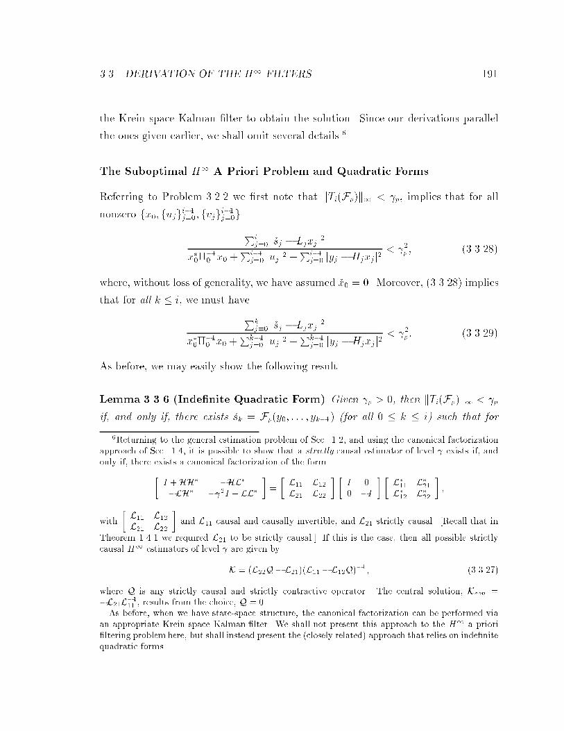
���� DERIVATION OF THE H� FILTERS ���
the Krein space Kalman �lter to obtain the solution� Since our derivations parallel
the ones given earlier� we shall omit several details��
The Suboptimal H� A Priori Problem and Quadratic Forms
Referring to Problem ��� we �rst note that kTi�Fp�k� � �p� implies that for all
nonzero fx�� fujgi��j��� fvjg
i��j��g
Pij�� j�sj � Ljxjj�
x������ x� �
Pi��j�� jujj
� �Pi��
j�� jyj �Hjxjj�� ��p � ����� �
where� without loss of generality� we have assumed �x� � �� Moreover� ����� � implies
that for all k � i� we must have
Pkj�� j�sj � Ljxjj�
x������ x� �
Pk��j�� jujj
� �Pk��
j�� jyj �Hjxjj�� ��p � �������
As before� we may easily show the following result�
Lemma ����� �Inde�nite Quadratic Form� Given �p � �� then kTi�Fp�k� � �p
if� and only if� there exists �sk � Fp�y�� � � � � yk��� �for all � � k � i� such that for
�Returning to the general estimation problem of Sec� ���� and using the canonical factorizationapproach of Sec� ���� it is possible to show that a strictly causal estimator of level � exists if� andonly if� there exists a canonical factorization of the form�
I �HH� �HL�
�LH� ���I � LL�
��
�L�� L��
L�� L��
� �I �� �I
� �L��� L���L��� L���
��
with
�L�� L��
L�� L��
�and L�� causal and causally invertible� and L�� strictly causal� �Recall that in
Theorem ����� we required L�� to be strictly causal�� If this is the case� then all possible strictlycausal H� estimators of level � are given by
K � L��Q� L�� L�� �L��Q ��� ����
where Q is any strictly causal and strictly contractive operator� The central solution� Kcen ��L��L
���� � results from the choice� Q � ��
As before� when we have state�space structure� the canonical factorization can be performed viaan appropriate Krein space Kalman �lter� We shall not present this approach to the H� a priori�ltering problem here� but shall instead present the closely related approach that relies on inde�nitequadratic forms�
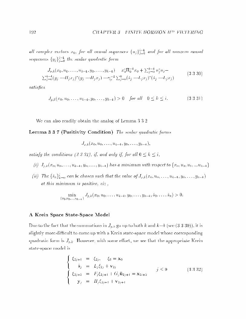
�� CHAPTER �� FINITE HORIZON H� FILTERING
all complex vectors x�� for all causal sequences fujgi��j�� and for all nonzero causal
sequences fyjgi��j�� the scalar quadratic form
Jp�k�x�� u�� � � � � uk��� y�� � � � � yk��� � x������ x� �
Pk��j�� u
�juj�Pk��
j���yj �Hjxj���yj �Hjxj�� ���p
Pkj����sj � Ljxj����sj � Ljxj�
��������
satis�es
Jp�k�x�� u�� � � � � uk��� y�� � � � � yk��� � � for all � � k � i� ��������
We can also readily obtain the analog of Lemma �����
Lemma ���� �Positivity Condition� The scalar quadratic forms
Jp�k�x�� u�� � � � � uk��� y�� � � � � yk����
satisfy the conditions � � � ��� if� and only if� for all � � k � i�
�i� Jp�k�x�� u�� � � � � uk��� y�� � � � � yk��� has a minimum with respect to fx�� u�� u�� ���uk��g�
�ii� The f�skgik�� can be chosen such that the value of Jp�k�x�� u�� � � � � uk��� y�� � � � � yk���
at this minimum is positive� viz��
minfx��u������uk��g
Jp�k�x�� u�� � � � � uk��� y�� � � � � yk��� �s�� � � � � �sk� � ��
A Krein Space StateSpace Model
Due to the fact that the summations in Jp�k go up to both k and k�� �see ���������� it is
slightly more di�cult to come up with a Krein state�space model whose corresponding
quadratic form is Jp�k� However� with some e�ort� we see that the appropriate Krein
state�space model is��� ��j�� � ��j� �� � x�
�sj � Lj��j � v�j��� ��j�� � Fj��j�� �Gj "u�j�� � x�i��
yj � Hj��j�� � v�j��
j � � �������
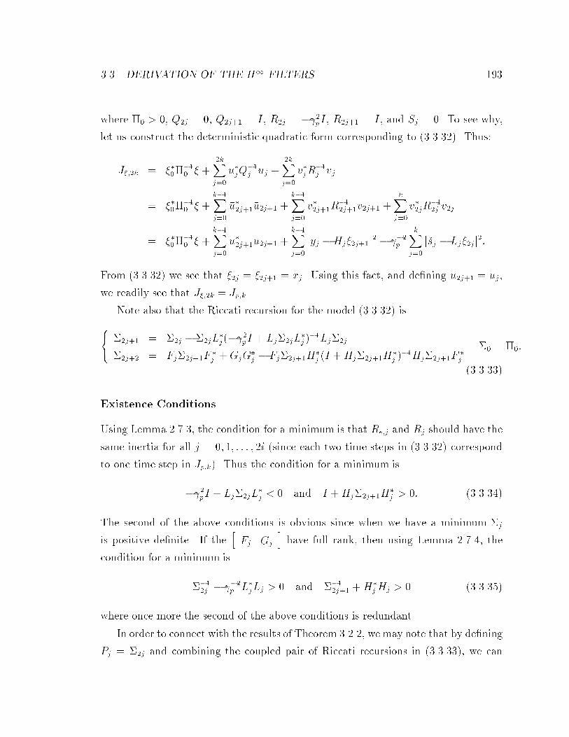
���� DERIVATION OF THE H� FILTERS ���
where �� � �� Q�j � �� Q�j�� � I� R�j � ���pI� R�j�� � I� and Sj � �� To see why�
let us construct the deterministic quadratic form corresponding to �������� Thus�
J���k � ������� � �
�kXj��
"u�jQ��j "uj �
�kXj��
v�jR��j vj
� ������� � �
k��Xj��
"u��j��"u�j�� �k��Xj��
v��j��R���j��v�j�� �
kXj��
v��jR���j v�j
� ������� � �
k��Xj��
"u��j��"u�j�� �k��Xj��
jyj �Hj��j��j� � ���p
kXj��
j�sj � Lj��jj��
From ������� we see that ��j � ��j�� � xj� Using this fact� and de�ning "u�j�� � uj�
we readily see that J���k � Jp�k�
Note also that the Riccati recursion for the model ������� is
��� #�j�� � #�j � #�jL
�j ���
�pI � Lj#�jL
�j ���Lj#�j
#�j�� � Fj#�j��F�j �GjG
�j � Fj#�j��H
�j �I �Hj#�j��H
�j ���Hj#�j��F
�j
#� � ���
��������
Existence Conditions
Using Lemma ����� the condition for a minimum is that Re�j and Rj should have the
same inertia for all j � �� �� � � � � i �since each two time steps in ������� correspond
to one time step in Jp�k�� Thus the condition for a minimum is
���pI � Lj#�jL�j � � and I �Hj#�j��H
�j � �� �������
The second of the above conditions is obvious since when we have a minimum #j
is positive de�nite� If thehFj Gj
ihave full rank� then using Lemma ���� the
condition for a minimum is
#���j � ���p L�jLj � � and #��
�j�� �H�jHj � � ��������
where once more the second of the above conditions is redundant�
In order to connect with the results of Theorem ���� we may note that by de�ning
Pj � #�j and combining the coupled pair of Riccati recursions in ��������� we can
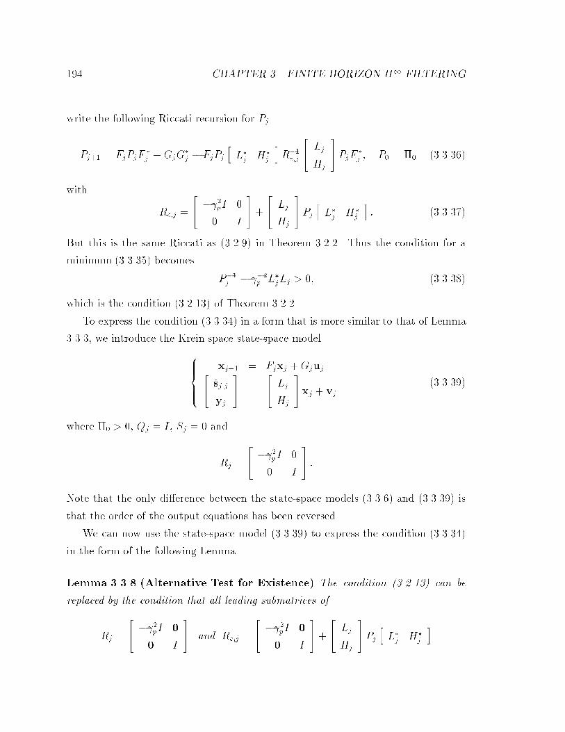
�� CHAPTER �� FINITE HORIZON H� FILTERING
write the following Riccati recursion for Pj
Pj�� � FjPjF�j �GjG
�j � FjPj
hL�j H�
j
iR��
e�j
�� Lj
Hj
��PjF
�j � P� � �� ��������
with
Re�j �
�� ���pI �
� I
���
�� Lj
Hj
��Pj
hL�j H�
j
i� ��������
But this is the same Riccati as ������ in Theorem ���� Thus the condition for a
minimum �������� becomes
P��j � ���p L�jLj � �� ������ �
which is the condition ������� of Theorem ����
To express the condition ������� in a form that is more similar to that of Lemma
������ we introduce the Krein space state�space model
���������
xj�� � Fjxj �Gjuj�� �sjjj
yj
�� �
�� Lj
Hj
��xj � vj
��������
where �� � �� Qj � I� Sj � � and
Rj �
�� ���pI �
� I
�� �
Note that the only di�erence between the state�space models ������� and �������� is
that the order of the output equations has been reversed�
We can now use the state�space model �������� to express the condition �������
in the form of the following Lemma�
Lemma ����� �Alternative Test for Existence� The condition � ���� � can be
replaced by the condition that all leading submatrices of
Rj �
�� ���pI
I
�� and Re�j �
�� ���pI
I
���
�� Lj
Hj
��Pj
hL�j H�
j
i

���� DERIVATION OF THE H� FILTERS ���
have the same inertia for all � � j � i� In other words�
���pI � LjPjL�j � � and I �Hj
�PjH�j � �
where �P��j � P��
j � ���p L�jLj � We no longer require thathFj Gj
ihave full rank�
and the size of the matrices involved is generally smaller than in � ������
Note that compared to Lemma ������ the condition in Lemma ���� is more strin�
gent since it requires that all leading submatrices of Rj and Re�j have the same inertia�
This distinction is especially important in square�root implementations of the H� �l�
ters �see �HSK�c� and Chapter ���
Construction of the H� a priori �lters
To complete the proof of Theorem ��� we still need to show that if a minimum over
fx�� u�� � � � � uk��g exists for all � � k � i� then we can �nd the estimates f�skgik�� such
that the value of Jp�k�x�� u�� � � � � uk��� y�� � � � � yk��� at its minimum is positive�
According to Theorem ���� the minimumvalue of Jp�k�x�� u�� � � � � uk��� y�� � � � � yk���
is
Pk��j��
he�s�j e�y�j
iR��
e�j
�� es�j
ey�j
��� e�s�k���
�pI � LkPkL
�k���es�k �
Pk��j��
�� �sj � �sjjj��
yj � �yjjj��
��� �� ���pI � LjPjL
�j LjPjH
�j
HjPjL�j I �HjPjH
�j
���� �� �sj � �sjjj��
yj � �yjjj��
��
���sk � �skjk��������pI � LkPkL
�k�����sk � �skjk��� � �
where �sjjj�� and �yjjj�� are obtained from the Krein space projections of �sj and yj onto
Lnf�slg
j��l�� � fylg
j��l��
o� respectively� Thus �sjjj�� is a linear function of fylg
j��l�� � Using
the block triangular factorization of the Re�j we may rewrite the above as
Pkj����sj � �sjjj���
�����pI � LjPjL�j �����sj � �sjjj����Pk��
j�� �yj � "yjjj�����I �Hj�PjH
�j ����yj � "yjjj��� � �
�������
where�� �sj � �sjjj��
yj � "yjjj��
�� �
�� I �
�HjPjL�j���
�pI � LjPjL
�j��� I
���� �sj � �sjjj��
yj � �yjjj��
�� � �������

��� CHAPTER �� FINITE HORIZON H� FILTERING
Or� in other words�
"yjjj�� � �yjjj�� �HjPjL�j ���
�pI � LjPjL
�j �����sj � �sjjj����
Note that "yjjj�� is given by the Krein space projection of yj ontonf�slg
jl��� fylg
j��l��
o�
Recall from Lemma ���� that
���pI � LjPjL�j � � � I �Hj
�PjH�j � ��
Any choice of �sjjj�� that renders ������� positive will do� and the simplest choice
is �sjjj�� � �sjjj�� � Lj�xjjj��� where �xjjj�� is given by the Krein space projection
of xj ontonf�slg
j��l�� � fyjg
j��l��
o� We may now utilize the Krein space Kalman �lter
corresponding to the state�space model �������� to recursively compute �xjjj��� viz��
�xj��jj � Fj�xjjj�� � FjPj
hL�j H�
j
iR��
e�j
�� �sj � Lj �xjjj��
yj �Hj �xjjj��
�� ������
Setting �sj � Lj �xjjj�� � � and simplifying we get the desired recursion for �xj��jj�
We should also mention here that in the a priori case the Lij of the canonical
spectral factorization are given by the following state�space representations��� L�� L��
L�� L��
�� �
��� Xi�� � AiXi �BiUi
Yi � CiXi �DiUi
�������
where�����������������������������������
Ai � Fi
Gi � Kp�i
�� �Ip �Hi
�PiH�i �
��� �HiPiL�i ���
�Iq � LiPiL�i �����
� ���Iq � LiPiL�i ����
��
Ci �
�� Hi
�Li
��
Di �
�� Ip �
� Iq
��
� ������
Note now that the transfer operator� L�� is strictly causal� Using the above state�space
representation� it is straightforward to show that the central �lter� Kcen � �L��L���� �

���� DERIVATION OF THE H� FILTERS ���
has state�space model given by the recursions of Theorem ���� It is also possible to
use the Lij �obtained above� to parametrize all possible H� �lters of level �� however�
we shall take a route similar to the one taken in Sec� �����
����� All H� A Priori Filters
The positivity condition ������� gives a full parametrization of all H� a priori esti�
mators� We thus have the following result�
Lemma ����� �All H� A Priori Estimators� All H� a priori estimators that
achieve a level �p �assuming they exist� are given by any �sj � Fp�j�y�� � � � yj��� that
satisfy
Pk��j��
�� yj �Hj �xj
�sj � Lj �xj
���
R��e�j
�� yj �Hj�xj
�sj � Lj�xj
��
���sk � Lk�xk�����pIq � LkPkL�k�����sk � Lk�xk� � ��
� � k � i �������
where �xj satis�es the recursion�
�xj�� � Fj�xj �Kp�j
�� yj �Hj �xj
�sj � Lj �xj
�� � �x� �������
with
Kp�j � FjPj
hH�
j L�j
iR��
e�j and Re�j �
�� Ip �
� ���pIq
���
�� Hj
Lj
��Pj
hH�
j L�j
i�������
and
Pj�� � FjPjF�j �GjQjG
�j �Kp�jRe�jK
�p�j� P� � ��� ����� �
We can also give a more explicit parametrization as follows�
Theorem ����� �All H� A Priori Estimators� All H� a priori estimators that
achieve a level �p �assuming they exist� are given by
�sj � Lj �xj � ���pI � LjPjL�j �
�
� �������
Sj
��I �Hj��
�Pj��H�j���
� �
� �yj�� �Hj��"xj���� � � � � �I �H��P�H
�� �� �
� �y� �H�"x���

�� CHAPTER �� FINITE HORIZON H� FILTERING
where
"xk � �xk � PkL�k���
�pI � LkL
�k�����sk � Lk�xk�� ��������
�xj satis�es the recursion
�xj��jj � Fj�xjjj�� � FjPj
hL�j H�
j
iR��
e�j
�� �sj � Lj�xjjj��
yj �Hj �xjjj��
�� � ��������
with Pj � �Pj and Re�j given by Theorem ����� and S is any �possibly nonlinear� con�
tractive causal mapping�
Proof� Referring to �������� we see that the "yjjj�� � Hj "xj di�er from �yjjj�� � Hj�xj�
via the additional projection onto �sjjj��� Thus we can write
"xjjj�� � �xjjj�� � PjL�j ���
�pI � LjPjL
�j �����sjjj�� � �sjjj����
which proves ��������� Moreover from the proof of Theorem ��� �see �������� the
recursion for �xj is given by ��������� Condition ������� can now be rewritten as
kXj��
��sjjj�� � �sjjj��������pI � LjPjL
�j �����sjjj�� � �sjjj��� �
k��Xj��
�yj � "yjjj�����I �Hj
�PjH�j ����yj � "yjjj��� � � �������
and an argument similar to the one given in the proof of Theorem ����� will yield the
desired result�
��� The H� Smoother
If instead of ef�k and ep�k� which correspond to the a posteriori and a priori �lters�
respectively� we consider the smoothed error
es�k � �skji � Lkxk� k � i

���� THE H� SMOOTHER ���
where �skji � Fs�y�� y�� � � � � yi� is the estimate of sk given all observations fyjg from
time � until time i� we are led to the so�calledH� smoothers� Such estimators guaran�
tee that the maximumenergy gain from the disturbancesn������ �x� � �x��� fuj� vjgij��
oto the smoothing errors fes�jgij�� is bounded by �s� i�e��
supx��u�h��v�h�
Pij�� e
�s�jes�j
�x� � �x��������x� � �x�� �
Pij�� u
�juj �
Pij�� v
�jvj
� ��s � ������
Using an argument similar to the ones given before� we are led to the following
quadratic form
Js�i�x�� u�� � � � � ui� y�� � � � � yi� � x����� x�� �
Pik�� u
�kuk�Pi
k���yk �Hkxk���yk �Hkxk�� ���Pi
k����skji � Lkxk����skji � Lkxk�������
Note that the only di�erence between Js�i and Jf�i is that �skjk has been replaced by
�skji �i�e�� �ltered estimates have been replaced by smoothed estimates�� Once more it
can be shown that an H� smoother of level �s will exist if� and only if� there exists
some �skji such that Js�i � �� The rather interesting result shown below� and which
has already been pointed out in the literature �see e�g�� �KN��� ST�� SFB���� is
that one H� smoother is given by the conventional H� smoother �which does not
even depend on the value of �s��
Theorem ����� �H� Smoother� For a given �s � �� an H� smoother that achieves
level �s exists� if� and only if� the block diagonal matrix
Re � Re�� Re�� � � �Re�i�
where
Re�j �
�� I �
� ���s
���
�� Hj
Lj
��Pj
hH�
j L�j
i
and Pj is the same as in Theorem ����� has �i���p positive eigenvalues and �i���q
negative eigenvalues� In other words� if� and only if�
In �Re� �h�i� ��p � �i� ��q
i�
If this is the case� one possible H� smoother is given by the H� smoother�

�� CHAPTER �� FINITE HORIZON H� FILTERING
Proof� The condition for Js�i�x�� u�� � � � � ui� y�� � � � � yi� to have a minimum is slightly
di�erent than the earlier cases� since we do not require that Js�k�x�� u�� � � � � uk� y�� � � � � yk�
have a minimum over the disturbances for all past values k � i� Thus using Lemma
���� the condition for a minimum over fx�� u�� � � � � uig is that the matrices
Re and R � R� R� � � �Ri
have the same inertia� where Rj � Ip ����sIq�� But this is precisely the inertia
condition given in the statement of the Theorem�
The value of Js�i at its minimum is �see Chapter �
hy� �s�ji
i�� Ry Ry�s
R�sy R�s
���� �� y
�sji
��
where we have de�ned �� Ry Ry�s
R�sy R�s
�� � h
�� y
�sji
�� ��� y
�sji
��i ������
with
y �
�����y����
yi
� � � �sji �
������s�ji���
�siji
� � � y �
�����y����
yi
� � � �sji �
������s�ji���
�siji
� � �
and where the fyjg and f�sjjig satisfy the Krein state�space model �������� In this
case all the entries in �sji are unknown and there is no causal dependence between the
f�sjjkg and the fyjg� Using a block triangular factorization� or a completion of squares
argument� the value at the minimum can be rewritten as
y�R��y y � ��sji �R�syR
��y y���R�s �R�syR
��y Ry�s�
����sji �R�syR��y y��
But Ry � � �since it is the covariance of a Hilbert space state�space model�� and
hence one possible choice of �sji to guarantee Js�i � � is to choose �sji � R�syR��y y � �sji�
which is clearly the H� smoothed estimate of �s�
The following result is now straightforward�

���� L�STEP H� PREDICTION ��
Theorem ����� �All H� Smoothers� All H� smoothers that achieve a level �s
�assuming they exist� are given by
�sji � �sji � ��R�s �R�syR��y Ry�s�
���S�R����y y� �����
where S is any �not necessarily causal� contractive mapping� �sji is the usual H�
smoothed estimate� and Ry and R�s �R�syR��y yRy�s are de�ned in � ��� ��
It is clear from the discussions so far in this chapter that the Krein space estimation
formalism provide simple derivations of H� estimators� These estimators turn out to
be certain Krein space Kalman �lters� and show that Krein space estimation yields
a uni�ed approach to H� and H� problems� To derive such �lters� and to solve
other related problems as discussed ahead� all one essentially needs is to identify an
inde�nite quadratic form� and to construct a convenient auxiliary state�space model
with the appropriate Gramians� Before considering further applications in the next
chapter� it will be useful to consider the problem of l�step H� prediction�
��� l�step H� Prediction
Consider once more the standard state�space model����������
xi�� � Fixi �Giui� x�
yi � Hixi � vi� i � �
si � Lixi
�������
where� as before� the initial condition x� and the disturbances fui� vig are unknown
quantities� yi is the observed output� and si is the signal we intend to estimate�
Suppose now that we would like to �nd l�step predictions of si� i�e�� estimates
�siji�l � Fl�i�y�� � � � � yi�l�� ������
that can only make use of the observations from time � to time i� l� where l � � is
some given value� �Obviously� l � � corresponds to the a priori �ltering problem just
considered�� In this case� our estimation errors will be the l�step prediction errors�
el�i � Lixi � �siji�l� �������
� CHAPTER �� FINITE HORIZON H� FILTERING
We can now de�ne the problem of �nding l�step H� predictors� Such predictors will
have the property that the maximum energy gain from the disturbances
n������ �x� � �x��� fujg
ij��� fvjg
i�lj��
o�
to the prediction errors
fel�jgij���
is bounded by some given �l� i�e��
supx��u�h��v�h�
Pij�� e
�l�jel�j
�x� � �x��������x� � �x�� �
Pij�� u
�juj �
Pi�lj�� v
�jvj
� ��l � ������
Note that in the above de�nition and inequality we have only included the measure�
ment disturbances vj until time i� l since measurement disturbances after time i� l
only a�ect the observations� fyj� j � i� lg� which the estimator is not allowed to use�
Before attempting to solve this H� prediction problem� let us see what happens
in the H� case� There to obtain� �xiji�l� one needs to project xi onto Lfyjgi�lj��� i�e��
the linear space spanned by the random variables� fy�� � � � � yi�lg� Using the state
equation in ������� this leads to
�xj��ji�l � Fj�xjji�l �Gj �ujji�l� �������
Now if we assume j � i�l� then �ujji�l � � �since uj is independent of the observations�
fykgi�lk���� This implies that
�xj��ji�l � Fj�xjji�l� j � i� l� �������
In other words� the predictions �xjji�l satisfy an �unforced� version of the same re�
cursion that the states� xj satisfy� Therefore to �nd �xiji�l� all one needs to do is
propagate the above recursion starting with the predicted estimate� �xi�l��� as the
initial condition� Thus� we may write
�xiji�l � Fi�� � � � Fi�l���xi�l��� �������
We shall presently see that the above expression is no longer true for l�step H�
predictions� It turns out that the recursion that needs to be propagated is slightly
more complicated�

���� L�STEP H� PREDICTION ��
To obtain the required H� estimates let us �rst note that ������ implies the
inequalities�
supx��u�h��v�h�
Pkj�� e
�l�jel�j
�x� � �x��������x� � �x�� �
Pkj�� u
�juj �
Pk�lj�� v
�jvj
� ��l � ����� �
for all k � �� � � � � i� This in turn implies that for all x� and for all fujgij�� �that are
not simultaneously zero�� we must be able to choose the �sjjj�l � Fl�i�y�� � � � � yj�l� such
that
Jl�k � �x� � �x�����
���x� � �x�� �kX
j��
u�juj �k�lXj��
v�jvj � ���l
kXj��
e�l�jel�j � �� �������
for all k � �� � � � � i� Of course� the above is true if� and only if�
�i� Jl�k has a minimum over the free variables fx�� fujgj��kg� for all k � �� � � � � i�
�ii� The �sjjj�l � Fl�i�y�� � � � � yj�l� can be chosen such that the value of Jl�k at this
minimum is positive �for all k � �� � � � � i��
Let us now proceed to check and construct the above two conditions recursively�
At time i � �� we have need to guarantee
Jl�k � �x�� �x�����
���x�� �x���u��u�����l ��s�j�l�L�x�����s�j�l�L�x�� � �� ��������
Now since �� � �� it is straightforward to see that we will have a minimum over the
free variables fx�� u�g if� and only if�
���l Iq � L���L�� � �� ��������
Moreover� the value at the minimum is given by
��s�j�l � L��x���h���l Iq � L���L
��
i����s�j�l � L��x��� �������
from which we readily infer that the �here� unique prediction is
�s�j�l � L��x�� ��������
Assume now that we have solved the problem until time k��� i�e�� we have checked
the condition for a minimum for all Jl�j from time j � � to time j � k � �� and have

� CHAPTER �� FINITE HORIZON H� FILTERING
chosen the f�sjjj�lgk��j�� such that the values of the Jl�j at their minima are positive�
We would now like to solve the problem for time k�
To this end� let us write Jl�k as
Jl�k � J�l�k � J�
l�k� �������
where
J�l�k � �x� � �x�����
���x� � �x�� �Pk�l
j�� u�juj�
Pk�lj��
�� yj �Hjxj
�sjjj�l � Ljxj
��� �� Ip �
� ����l Iq
���� yj �Hjxj
�sjjj�l � Ljxj
�� ��������
and
J�l�k �
kXj�k���l
u�juj �kX
j�k���l
���l ��sjjj�l � Ljxj����sjjj�l � Ljxj�� ��������
The reason why we have decomposed Jl�k in this fashion is that J�l�k is a function of
fx�� u�� � � � � uk�lg� or equivalently� fu�� � � � � uk�l� xk�l��g� i�e��
J�l�k � J�
l�k�u�� � � � � uk�l� xk�l���� ��������
and J�l�k is a function of fxk�l��� uk�l��� � � � � ukg� i�e��
J�l�k � J�
l�k�xk�l��� uk�l��� � � � � uk�� ������ �
Thus� in e�ect� the above decomposition decouples the e�ects of fuj� j � k � lg and
fuj� j � k � lg and allows us to minimize over the two sets separately�
Now the condition that J�l�k have a minimum over fuj� j � k � lg is readily seen
to be that the matrices
Re�j �
�� Ip �
� ���l Iq
���
�� Hj
Lj
��Pj
hH�
j L�j
iand
�� Ip �
� �Iq
�� ��������
have the same inertia for all j � �� � � � k � l� where Pj satis�es the Riccati recursion
Pj�� � FjPjF�j �GjG
�j � FjPj
hH�
j L�j
iR��
e�j
�� Hj
Lj
�� � P� � ��� �������

���� L�STEP H� PREDICTION ��
Moreover the minimum value is
J�l�k�min� �
k�lXj��
�� yj �Hj�xj
�sjjj�l � Lj�xj
���
R��e�j
�� yj �Hj �xj
�sjjj�l � Lj�xj
��� �x�k���lP
��k���l�x
�k���l�
�������
where �xj satis�es the Krein space Kalman �lter recursions�
�xj�� � Fj�xj �Kp�j
�� yj �Hj�xj
�sjjj�l � Lj�xj
�� � �x� � �x� ������
with
Kp�j � FjPj
hH�
j L�j
iR��
e�j � �������
Since the �rst term �i�e�� the summation� in J�l�k�min� is independent of xk���l� to
minimize Jl�k over the remaining variables fxk�l��� uk�l��� � � � � ukg it su�ces to mini�
mize
J�l�k � �x�k���lP
��k���l�x
�k���l �
�x�k���lP��k���l�x
�k���l �
Pkj�k���l u
�juj �
Pkj�k���l �
��l ��sjjj�l � Ljxj����sjjj�l � Ljxj�
������
over those variables� But the condition for this minimum is readily seen to be
Rk���le�j
�� ���l Iq � LjP
k���lj L�j � �� j � k � � � l� � � � � k �������
where Pj�k���l satis�es the Riccati recursion
P k���lj�� � FjP
k���lj F �
j �GjG�j�FjP
k���lj L�j
hRk���l
e�j
i��LjP
k���lj F �
j � P k���lk���l � Pk���l�
�������
Moreover� in this case the value at the minimum is given by
kXj�k���l
��sjjj�l � Lj�xk���lj ��
hRk���l
e�j
i����sjjj�l � Lj �x
k���lj �� �������
where �xk���lj satis�es the Krein space Kalman �lter recursions��
�xk���lj�� � Fj�x
k���lj �Kk���l
p�j ��sjjj�l � Lj �xk���lj �� j � k � �� l� � � � k ����� �
�Note that at time k all the �sjjj�l for j � k � �� l� � � �k in the given recursion are known�

�� CHAPTER �� FINITE HORIZON H� FILTERING
where
Kk���lp�j � FjP
k���lj L�j
hRk���l
e�j
i��� �������
Therefore the value of Jl�k at it its minimum is given by
Jl�k�min� �Pk�l
j��
�� yj �Hj �xj
�sjjj�l � Lj �xj
���
R��e�j
�� yj �Hj�xj
�sjjj�l � Lj �xj
���
Pkj�k���l��sjjj�l � Lj �x
k���lj ��
hRk���l
e�j
i����sjjj�l � Lj �x
k���lj ��
��������
Now if we de�ne
A�� Jl�k�min�� ��skjk�l � Lj �x
k���lk ��
hRk���l
e�k
i����skjk�l � Lj�x
k���lk �� ��������
then it possible to show that A � �� Indeed�
A �k�lXj��
�� yj �Hj �xj
�sjjj�l � Lj �xj
���
R��e�j
�� yj �Hj �xj
�sjjj�l � Lj �xj
���
k��Xj�k�l
��sjjj�l � Lj�xk���lj ��
hRk���l
e�j
i����sjjj�l � Lj �x
k���lj �
�k�l��Xj��
�� yj �Hj�xj
�sjjj�l � Lj�xj
���
R��e�j
�� yj �Hj �xj
�sjjj�l � Lj�xj
���
minxk�l�uk�l�����uk��
���x�k�lP
��k�l�xk�l � v�k�lvk�l �
k��Xj�k�l
u�juj �k��X
j�k�l
���l e�l�jel�j
��
�k�l��Xj��
�� yj �Hj�xj
�sjjj�l � Lj�xj
���
R��e�j
�� yj �Hj �xj
�sjjj�l � Lj�xj
���
minxk�l�uk�l�����uk��
���x�k�lP
��k�l�xk�l �
k��Xj�k�l
u�juj �k��X
j�k�l
���l e�l�jel�j
��
� Jf�k���min� � ��
�Note that in the last step we have made use of the fact that the f�sjjj�lgk��j�� were
chosen such that Jf�k���min� � ��
Thus writing�
Jl�k�min� � A� ��skjk�l � Lj �xk���lk ��
hRk���l
e�k
i����skjk�l � Lj�x
k���lk ��
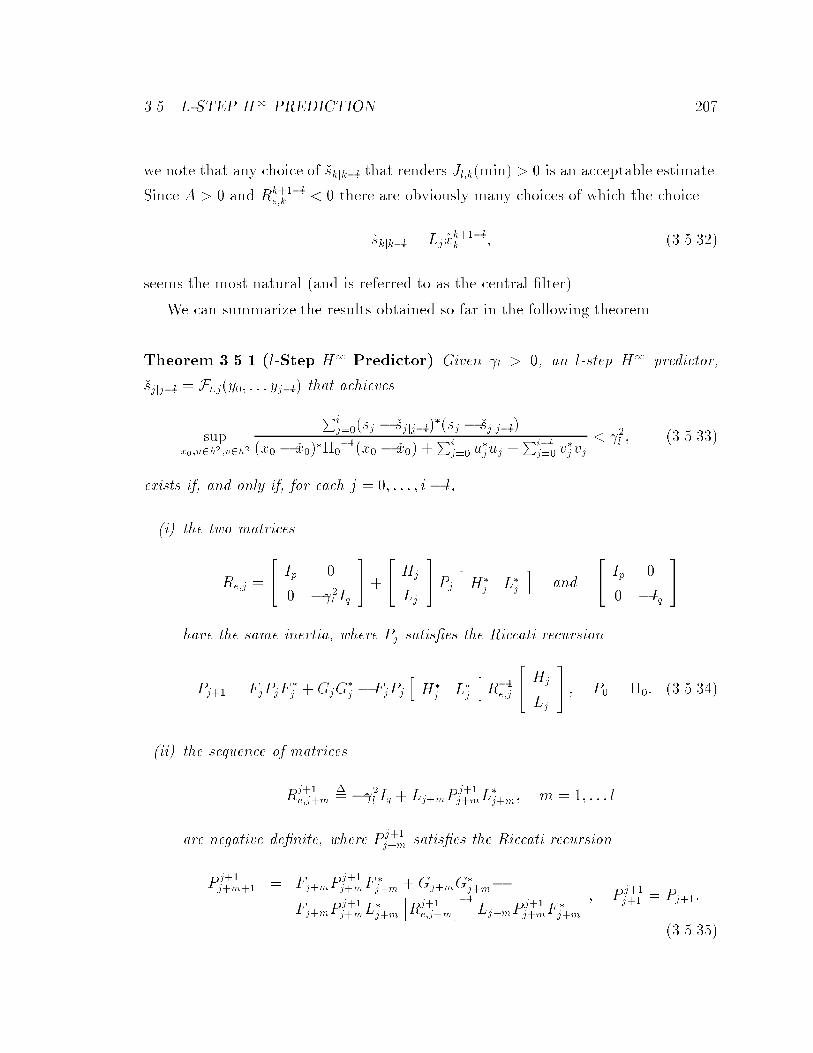
���� L�STEP H� PREDICTION ��
we note that any choice of �skjk�l that renders Jl�k�min� � � is an acceptable estimate�
Since A � � and Rk���le�k � � there are obviously many choices of which the choice
�skjk�l � Lj�xk���lk � �������
seems the most natural �and is referred to as the central �lter��
We can summarize the results obtained so far in the following theorem�
Theorem ����� �lStep H� Predictor� Given �l � �� an l�step H� predictor�
�sjjj�l � Fl�j�y�� � � � yj�l� that achieves
supx��u�h��v�h�
Pij���sj � �sjjj�l�
��sj � �sjjj�l�
�x� � �x��������x� � �x�� �
Pij�� u
�juj �
Pi�lj�� v
�j vj
� ��l � ��������
exists if� and only if� for each j � �� � � � � i� l�
�i� the two matrices
Re�j �
�� Ip �
� ���l Iq
���
�� Hj
Lj
��Pj
hH�
j L�j
iand
�� Ip �
� �Iq
��
have the same inertia� where Pj satis�es the Riccati recursion
Pj�� � FjPjF�j �GjG
�j � FjPj
hH�
j L�j
iR��
e�j
�� Hj
Lj
�� � P� � ��� �������
�ii� the sequence of matrices
Rj��e�j�m
�� ���l Iq � Lj�mP
j��j�mL
�j�m� m � �� � � � l
are negative de�nite� where P j��j�m satis�es the Riccati recursion
Pj��j�m�� � Fj�mP
j��j�mF
�j�m �Gj�mG
�j�m�
Fj�mPj��j�mL
�j�m
hRj��
e�j�m
i��Lj�mP
j��j�mF
�j�m
� P j��j�� � Pj���
��������

� CHAPTER �� FINITE HORIZON H� FILTERING
If this is the case then one possible l�step H� predictor is given by�
�sj�ljj � Lj�l�xj��j�l � ��������
where �xj��j�m satis�es the recursion�
�xj��j�m�� � Fj�m�xj��j�m �K
j��p�j�m��sj�mjj�m�l � Lj�m�x
j��j�m�� �xj��j�� � �xj�� ��������
with
Kj��p�j�m � Fj�mP
j��j�mL
�j�m
hRj��
e�j�m
i��� ������ �
and where �xj satis�es the recursion�
�xj�� � Fj�xj �Kp�j
�� yj �Hj�xj
�sjjj�l � Lj �xj
�� � �x� � �x� ��������
with
Kp�j � FjPj
hH�
j L�j
iR��
e�j � �������
Remark� It will be useful to further explain the structure of the l�step H� �lter
given in the above theorem�
�� Set �skjk�l � LkFk�� � � � F��x� for k � �� � � � � l� ��
� Set j � �� �j is the observation index that runs from � to i� l��
�� Check inertia condition �i�� Compute Pj�� �using �������� and �xj�� �using
����������
� Perform the l�step propagation of the Riccati variable� P j��j�m� �using ���������
and check the negativity conditions �ii��
�� Perform the l�step propagation of �xj��j�m �using ��������� to �nd the estimate�
�sj�ljj � Lj�l�xj��j�l �
We also have �skjk�l � LkFk�� � � � F�x for k � �� � � � � l� ��

���� CONCLUSION ��
�� Set j � j � � and go to ��
The important feature of the l�step H� predictor is that at each iteration �i�e��
after each observation� in addition to propagating one step of the usual Riccati recur�
sion ������� and state estimate recursion ��������� �which are the same recursions as
those of the a posteriori �lter� we need to propagate l steps of the auxiliary Riccati
recursion for P i��i�m and l steps of the auxiliary state estimate� �xi��i�m� This is clearly
di�erent from the case of l�step H� prediction�
It is also straightforward to parametrize all possible l�step H� predictors of a
given level �l�
Lemma ����� �All lStep H� Predictors� All l�step H� predictors that achieve
a level �l �assuming they exist� are given by any �sjjj�l � Fl�j�y�� � � � yj�l� that satisfy
Pk�lj��
�� yj �Hj �xj
�sjjj�l � Lj�xj
���
R��e�j
�� yj �Hj �xj
�sjjj�l � Lj �xj
���
Pkj�k���l��sjjj�l � Lj �x
k���lj ��
hRk���l
e�j
i����sjjj�l � Lj �x
k���lj � � �
k � �� � � � � i
�������
where �xj��j�m and �xj satisfy the recursions
�xj��j�m�� � Fj�m�xj��j�m �Kj��
p�j�m��sj�mjj�m�l � Lj�m�xj��j�m�� �xj��j�� � �xj�� ������
and
�xj�� � Fj�xj �Kp�j
�� yj �Hj�xj
�sjjj�l � Lj �xj
�� � �x� � �x� �������
respectively� and where Rk���le�j � Re�j� K
j��p�j�m and Kp�j as in Theorem �����
��� Conclusion
Certain studies in least�squares estimation� adaptive �ltering and H� �ltering moti�
vated us to develop a theory for linear estimation in certain inde�nite metric spaces�
called Krein spaces� The main di�erence from the conventional Hilbert space frame�
work for Kalman �ltering and LQG control are that projections in Krein spaces may

�� CHAPTER �� FINITE HORIZON H� FILTERING
not necessarily exist or be unique� and that quadratic forms may have stationary
points that are not necessarily extreme points �i�e�� minima or maxima�� We showed
that these simple but fundamental di�erences explain both the unexpected similar�
ities and di�erences between the well�known Kalman �lter solution for stochastic
state�space systems and the solution for the completely nonstochastic H� �ltering
problem�
The main points are the following� There are many problems whose solution can be
reduced to the recursive minimization of some inde�nite quadratic form� A stationary
point� when it exists� of the quadratic form can be computed as follows� set up a
�partially equivalent� problem of projecting a vector in a Krein space onto a certain
subspace� The advantage is that when there is state�space structure� this projection
can be recursively computed by using the innovations approach to derive a Krein space
Kalman �lter� The equivalence is only partial because the Krein space projection
only de�nes the stationary point of the quadratic form and further conditions need
to be checked to determine if this point is also a minimum� It turns out that this
checking can also be done recursively using quantities arising in the Kalman �ltering
algorithms�
Apart from quite straightforward derivations of known results in H�� H� and
risk�sensitive estimation and control� the above approach allows us to extend to the
H� setting some of the huge body of results and insights developed over the last
three decades in the �eld of Kalman �ltering �and LQG control�� A �rst bonus is the
derivation �see �HSK�c� and Chapter �� of square�root and �fast� Chandrasekhar
algorithms for H� estimation and control� a possibility that is much less obvious
in current approaches� These square�root algorithms� which are now increasingly
standard inH� Kalman �ltering� have two advantages over the earlierH� algorithms�
they eliminate the need for explicitly checking the existence conditions of the �lters�
and have various potential numerical and implementational advantages�
Application of the Krein space formulation to adaptive �ltering arises from the
approach in �SK�b� where it was shown how to recast adaptive �ltering problems as
state�space estimation problems� If we further allow the elements of the state�space
model to belong to a Krein space� then we can solve �nite memory and H� adaptive

���� CONCLUSION ��
�ltering problems� In the �nite memory case� this allows us to consider general sliding
patterns with windows of varying lengths� In the H� adaptive case� this has allowed
us to establish that the famed LMS �or stochastic gradient� algorithm is an optimal
H� �lter �HSK��a� �see also Chapter ���
We also remark that� although not pursued here� it is also possible to construct
dual �rather than partially equivalent� Krein state�space models �via the concept of a
dual basis�� which can be used to extend the methods to the solution of H� and H�
control problems� This will be done in Chapter ��

Chapter �
Further Applications
In this chapter we show that several interesting problems in risk�sensitive estimation
and control� dynamic quadratic game theory� and �nite memory adaptive �ltering
follow as special cases of the Krein space linear estimation theory developed in Chap�
ter �� The major point is that all these problems can be cast into the problem of
calculating the stationary point of certain inde�nite quadratic forms� and that by
considering the appropriate state space models and error Gramians� we can use the
Krein space estimation theory to calculate these stationary points and study their
properties� The approach discussed here allows for interesting generalizations� such
as �nite memory adaptive �ltering with varying sliding patterns and suboptimal re�
cursive total least�squares algorithms�
��� Introduction
The classical Kalman �lter can be viewed as a recursive procedure that minimizes
the expected value of a certain quadratic cost function� Recently there has also
been increasing interest in an alternative so�called exponential�quadratic cost function
�Jac�� SDJ�� Whi��� SFB�� � and estimators �and controllers� that minimize its
expected value� The ensuing theory is sometimes called LEQG �linear�exponential�
quadratic�Gaussian� theory to re�ect the facts that the resulting optimal estimators
�and controllers� are linear� the cost function is the exponential of a quadratic� and the
���

���� INTRODUCTION ��
disturbances are assumed to be Gaussian random variables� It is also called �following
Whittle� risk�sensitive estimation and control� since the criterion is risk�sensitive� in
the sense that it depends on a real parameter that determines whether more or less
weight should be given to higher or smaller errors� �Roughly speaking when more
weight is given to smaller errors the criterion is risk�seeking� and when more weight
is given to large errors the criterion is risk�averse� The �lters obtained within this
framework are termed risk�sensitive and include the conventional Kalman �lter as a
�so�called risk�neutral� special case�
Following some pioneering work in game theory �motivated primarily by the �eld
of economics �NM� KT�� �� since the mid �����s there has been considerable in�
terest in applying game�theoretic ideas and methods to estimation and control� In
this framework� the problem of estimation �or control� is treated as a noncooperative
two�player game� with one player �the opponent� being the exogenous signals� and the
other player being the estimator �or controller�� This approach� which treats the ex�
ogenous signals as malignant disturbances that compete against the estimator �or con�
troller�� is� of course� fundamentally di�erent from the H� �or risk�sensitive� approach
where the exogenous signals are simply taken to be random variables with known
probability distributions� The class of games most often applied to estimation and
control is the class of di�erential games with quadratic payo� �Isa��� Ber�� BH�� �
which� in the discrete�time case of interest to us� shall henceforth be referred to as a
quadratic dynamic game� One reason for its pervasive use may be that the solutions
to quadratic dynamic games bear many similarities to the solutions of H� estimation
and control � estimators have an observer structure� full information controllers have
state�feedback structure� the various observer and state�feedback gains are found from
the solution of certain Riccati equations� etc�
In fact� it has recently been shown that there is a close connection between H�
estimation and control� game theory� and risk�sensitive estimation and control �GD���
Bas��� LAKG�� � Indeed� it turns out the central H� estimators and controllers� as
well as the risk�sensitive optimal estimators and controllers can be derived as solutions
to a certain quadratic dynamic game� �This observation is the driving force of the
game�theoretic approach to H� control�

�� CHAPTER �� FURTHER APPLICATIONS
In this chapter we shall shed further light on the connections between these theo�
ries by using the Krein space approach of Chapter �� Indeed� we shall see that� as with
H� estimation and control� risk�sensitive estimation and control problems� quadratic
games� and �nite memory adaptive �ltering problems lead almost by inspection to
inde�nite deterministic quadratic forms� Following Chapters � and � we can solve
these problems by constructing the corresponding Krein space models� Once this is
done� the Krein space Kalman �lter solutions can be written down immediately� and
the existence conditions for the problem can also be expressed in terms of quantities
easily related to the basic Riccati equations of the Kalman �lter�
The remainder of the chapter is organized as follows� In Section �� we describe
the problem of risk�sensitive estimation� and show that a risk�sensitive estimator is
one that computes the stationary point of a certain �possibly inde�nite� quadratic
form� provided that this quadratic form has a minimum over a certain set of variables�
By considering a corresponding Krein state space model� we use the results of Chapter
� to derive conditions for the existence of the minimum� and to show that the Krein
space projection also solves the risk�sensitive estimation problem� We then derive
risk�sensitive a posteriori� a priori� smoothed� and l�step ahead �lters parallel to what
was done in Chapter � Sec� � gives a very brief introduction to the theory of
quadratic dynamic games� We show that such games lend themselves to analysis by
Krein space methods since the cost �or payo�� function in is an inde�nite quadratic
form� Moreover� we show that the �max�min� min�max� or saddle point� solutions
to such games are found by stationarizing these quadratic forms and checking for
certain minimizing and maximizing conditions� Some speci�c examples from state�
space estimation and control are also provided� Finite memory adaptive �ltering is
studied in Sec� �� where the Krein space approach is used to solve this problem� and
to connect it to state�space approaches to adaptive �ltering� An interesting byproduct
of our analysis is the physical interpretation of innovations with negative Gramian as
corresponding to the loss of information� The chapter is concluded in Sec� �� with
some remarks on further applications of the Krein space framework� e�g�� to recursive
solutions of �suboptimal� total least�squares problems�
���� RISK�SENSITIVE ESTIMATION ���
��� Risk�Sensitive Estimation
The so�called risk�sensitive �or exponential cost� criterion was introduced in �Jac�
and further studied in �SDJ�� Whi��� SFB�� � Glover and Doyle �GD�� noticed
their close connection to the H� �lters of Chapter � We shall make this connection
in a di�erent way by introducing an appropriate quadratic form�
����� The Exponential Cost Function
We again start with a state�space model of the form
��� xj�� � Fjxj � Gjuj � j � �
yj � Hjxj � vj
������
However� we now assume that the initial condition� x�� and the driving and mea�
surement disturbances� fujg� and fvjg are independent zero mean Gaussian random
variables with covariances with
E
�����x�
ui
vi
����hx�� u�j v�j
i�
������� � �
� Qi�ij �
� � Ri�ij
���� � ������
As we have seen in Sec� ��� conventional H� estimators� such as the Kalman �l�
ter� estimate the quantity sj � Ljxj from the observations fykgmk�� �i�e�� �sjjm �
Fi�y�� � � � �ym�� by performing the following minimization
minf�sjjmg
E �Ci �����
whereCi��Pi
j����sjjm�Ljxj����sjjm�Ljxj� and E �� denotes expectation� As we have
seen earlier� the choices m � j� m � j � �� m � i� and m � j � l correspond to the
a posteriori� the a priori� the smoothed� and the l�step ahead� estimation problems�
respectively� Moreover� the expectation is taken over the jointly Gaussian random
variables fx�� fujgij��� fyjgij��g�� Using the fact that x� and the fujg and fvjg are
independent Gaussian random variables with covariances given by ������� and the
�Note that this set of random variables is equivalent to the set fx�� fujgij��� fvjg
ij��g�

��� CHAPTER �� FURTHER APPLICATIONS
fact that vj � yj �Hjxj� allows us to write the joint probability distribution of the
fx�� fujgij��� fyjgij��g as
p�x��u�� � � � � ui� y�� � � � � yi� � exp��
�Ji�x��u�� � � � � ui� y�� � � � � yi�
������
where the symbol � stands for �proportional to� and Ji�x��u�� � � � � ui� y�� � � � � yi� is
given by
x������ x� �
iXj��
u�jQ��j uj �
iXj��
�yj �Hjxj��R��
j �yj �Hjxj�� ������
In the terminology of �Whi�� � any �lter that minimizes ����� is known as a risk�
neutral �lter�
An alternative criterion that is risk�sensitive has been extensively studied in
�Jac�� SDJ�� Whi��� SFB�� and corresponds to the minimization problem
minf�sjjmg
�i��� � minf�sjjmg
���
�log
Eexp��
�
�Ci�
��� ������
The criterion in ������ is known as an exponential cost criterion� and any �lter that
minimizes �i��� is referred to as a risk�sensitive �lter�� The scalar parameter � is
correspondingly called the risk�sensitivity parameter� Some intuition concerning the
nature of this modi�ed criterion is obtained by expanding �i��� in terms of � and
writing�
�i��� � E�Ci���
V ar�Ci� �O�����
The above equation shows that for � � �� we have the risk�neutral case �i�e�� con�
ventional H� estimation�� When � � �� we seek to maximize Eexp�� ��Ci�� which is
convex and decreasing in Ci� Such a criterion is termed risk�seeking �or optimistic�
since larger weights are on small values of Ci� and hence we are more concerned with
the frequent occurrence of moderate values of Ci than with the occasional occurrence
of large values� When � � �� we seek to minimize Eexp�� ��Ci�� which is convex
and increasing in Ci� Such a criterion is termed risk�averse �or pessimistic� since
large weights are on large values of Ci� and hence we are more concerned with the
�Such �lters are also called LEQG �linear�exponential�quadratic�Gaussian� �lters to re�ect thefacts that� as we shall momentarily see� the optimum �lter is linear� the cost is the exponential of aquadratic� and the disturbances are Gaussian�

���� RISK�SENSITIVE ESTIMATION ���
occasional occurrence of large values than with the frequent occurrence of moderate
ones� In what follows� we shall see that in the risk�averse case � � �� the limit at
which minimizing ������ makes sense corresponds to the optimal H� criterion� �To
further compare the risk neutral and risk�averse approaches to estimation we have
plotted the cost functions �whose expected values are to be minimized� for these two
approaches in Fig� �� �the risk�averse case corresponds to � � ��� As can be seen in
the risk�averse case we incur �exponentially� larger costs for large values of Ci�
0 0.2 0.4 0.6 0.8 1 1.2 1.4 1.6 1.8 20
1
2
3
4
5
6
7
cost
Comparison of Risk Neutral and Risk−Averse Cost Functions
C i
I
III: cost = C
i
II: cost = exp(C ) − 1i
Figure ��� Comparison of risk neutral and risk�averse cost functions�
����� Minimizing the Risk�Sensitive Criterion
Using the probability density function ����� we can easily verify that
E
exp��
�
�Ci�
��
Zexp��
�
�Ci�exp
��
�Ji�x��u�� � � � � ui� y�� � � � � yi�
�dx�
iYk��
duk
iYk��
dyk�

��� CHAPTER �� FURTHER APPLICATIONS
which� upon a change in the order of the integrations� becomes
E�exp���
�Ci�� �
Z iYk��
dyk
Zexp
��
�fJi�x��u�� � � � � ui� y�� � � � � yi� � �Cig
�dx�
iYk��
duk�
������
Since the f�zjjmg are functions of the observations fykgmk��� the above relation shows
that the risk�sensitive criterion ������ can be alternatively written as
�i� For � � ��
maxf�sjjmg
Zexp
��
�fJi�x��u�� � � � � ui� y�� � � � � yi� � �Cig
�dx�
iYk��
duk�
�ii� For � � ��
minf�sjjmg
Zexp
��
�fJi�x��u�� � � � � ui� y�� � � � � yi� � �Cig
�dx�
iYk��
duk�
This suggests that we de�ne the second�order scalar form
Ji�x�� u�� � � � � ui�� � � � � � yi��� Ji�x�� u�� � � � � ui�� � � � � � yi� � �Ci �
x������ x��
iXj��
u�jQ��j uj�
iXj��
�yj�Hjxj��R��
j �yj�Hjxj���iX
j��
��sjjj���Ljxj����sjjj���Ljxj�
Before proceeding with the extremizations in �i� and �ii�� we need to ensure that
the integrals in �i� and �ii� be �nite� The condition is given by the following Lemma�
which is easy to prove�
Lemma ����� �Finiteness Condition� The integral
Zexp
��
� Ji�x��u�� � � � � ui� y�� � � � � yi�
�dx�
iYk��
duk�
is �nite if� and only if� Ji�x�� u�� � � � � ui� y�� � � � � yi� has a minimum over fx�� u�� � � � � uig�
In this case the value of the integral is proportional to
exp���
�minx��u
Ji�x�� u�� � � � � ui� y�� � � � � yi���

���� RISK�SENSITIVE ESTIMATION ���
The above Lemma thus reduces the risk�sensitive problem to one of �nding the
minimum of a scalar quadratic form� More precisely� the criterion becomes
�i� For � � ��
minf�sjjlg
minx��u
Ji�x�� u�� � � � � ui� y�� � � � � yi��
�ii� For � � ��
maxf�sjjlg
minx� �u
Ji�x�� u�� � � � � ui� y�� � � � � yi��
It is noteworthy that the second of the above problems is a quadratic dynamic
game �see e�g�� �Isa��� BB�� �� We shall �very� brie�y study quadratic game theory in
Sec� � and shall show that they can also be solved using the Krein space approaches
developed in Chapters � and �
For the time being� however� let us return to the above risk�sensitive problems� In
order to solve them� we can introduce the following auxiliary Krein state�space model
that corresponds to the �possibly inde�nite� quadratic form Ji�x�� u�� � � � � ui�� � � � � � yi�����������
xj�� � Fjxj �Gjuj j � ��� yi
�sijl
� �
�� Hi
Li
�xi � vi
������
with
h
�����x�
uj
vj
���� ������x�
uk
vk
����i �
��������
�� � �
� Qi�ij �
� �
�� Rj �
� ���I
� �jk
�������� ������
We can now readily use the state�space model ������� and the results of the earlier
Chapters � and � to check for the condition of a minimum over fx�� u�� � � � � uig� and
to compute the value at the minimum� Since we have provided the details in those
earlier chapters� here we shall only brie�y outline the steps for the a posteriori risk�
sensitive estimation problem��
�Indeed the derivations are almost identical to those of the H� �lters of Chapter �since the quadratic form Ji�x�� u�� � � � � ui� y�� � � � � yi� is exactly the same as the quadratic formsJf�i�x�� u�� � � � � ui� y�� � � � � yi�� Jp�i�x�� u�� � � � � ui� y�� � � � � yi� and Js�i�x�� u�� � � � � ui� y�� � � � � yi�� whenwe choose � � ���f � � � ���p and � � ���s � and when the estimate is chosen as a �ltered� predicted
and smoothed estimate� respectively�

��� CHAPTER �� FURTHER APPLICATIONS
First note that when � � �� the quadratic form Ji�x�� u�� � � � � ui�� � � � � � yi� is non�
negative so that it always has a minimum� Thus risk�seeking optimal �lters �corre�
sponding to � � �� always exist� On the other hand� when � � �� the quadratic
form Ji�x�� u�� � � � � ui�� � � � � � yi� is� in general� inde�nite� so that further conditions are
required for a minimum to exist� This condition is given by the requirement that the
matrices�
�� Rj �
� ���I
� and Re�j �
�� Rj �
� ���I
��
�� Hj
Lj
�Pj
hH�
j L�j
i�������
have the same inertia for all j � �� � � � i� where P� � ��� and
Pj�� � FjPjF�j �GjQjG
�j � FjPj
hH�
j L�j
iR��
e�j
�� Hj
Lj
�PiF
�i � �������
In both cases� the value of Ji�x�� u�� � � � � ui� y�� � � � � yi� at its minimum is given by
Ji�min� �iX
j��
�� yj �Hj !xj
�sjjj � Lj !xj
��
R��e�j
�� yj �Hj!xj
�sjjj � Lj!xj
� � �������
where !xj obeys the Krein space Kalman �lter recursion�
!xj�i � Fj!xj �Kp�j
�� yj �Hj !xj
�sjjj � Lj !xj
� � !x� � � ������
with Kp�j � FjPj
hH�
j L�j
iR��
e�j � Using a block LDU �lower�diagonal�upper� trian�
gular factorization of the matrix� Re�j � and de�ning the Schur complement�
"j � ���I � LjPjL�j � LjPjH
�j �Rj �HjPjH
�j ���HjPjL
�j � ������
and the estimate�
!sjjj � Lj !xj � LjPjH�j �Rj �HjPjH
�j ����yj �Hj!xj�� �������
allows us to write
Ji�min� �iX
j��
�� yj �Hj !xj
�sjjj � !sjjj
�� �� R��
j �
� "��j
��� yj �Hj !xj
�sjjj � Lj!xj
� � �������

���� RISK�SENSITIVE ESTIMATION ���
Thus in the risk�seeking case �� � ��� our problem becomes�
minf�sjjjg
iXj��
�� yj �Hj !xj
�sjjj � !sjjj
�� �� R��
j �
� "��j
��� yj �Hj!xj
�sjjj � Lj!xj
� � �������
and in the risk�averse case �� � ���
maxf�sjjjg
iXj��
�� yj �Hj !xj
�sjjj � !sjjj
�� �� R��
j �
� "��j
��� yj �Hj!xj
�sjjj � Lj!xj
� � �������
But when � � �� we have Re�j � �� and thus "j � �� Therefore the quadratic form
in ������� has a minimum over the f�sjjjg which is readily given by
�sjjj � !sjjj� �������
Likewise� when � � �� due to the inertia condition on Re�j� we have "j � �� Thus� in
this case� the quadratic form in ������� has a maximum over the f�sjjjg which is also
given by
�sjjj � !sjjj� �������
As in Chapter it is also possible to give a recursion for the !xjjj which yields Lj!xjjj �
!sjjj� This leads to the following result�
Theorem ����� �A Posteriori Risk�Sensitive Filter� Consider the a posteriori
risk�sensitive estimation problem�
minf�sjjjg
��
�log
��Eexp
����
�
iXj��
�sj � !sjjj���sj � !sjjj�
�A� �
for some given �� When � � �� the risk�sensitive estimation problem always has a
solution� When � � �� a solution exists if� and only if� the matrices�� Rj �
� ���I
� and Re�j �
�� Rj �
� ���I
��
�� Hj
Lj
�Pj
hH�
j L�j
i
have the same inertia for all j � �� �� � � � i� where P� � �� and
Pj�� � FjPjF�j �GjQjG
�j � FjPj
hH�
j L�j
iR��
e�j
�� Hj
Lj
�PiF
�i �
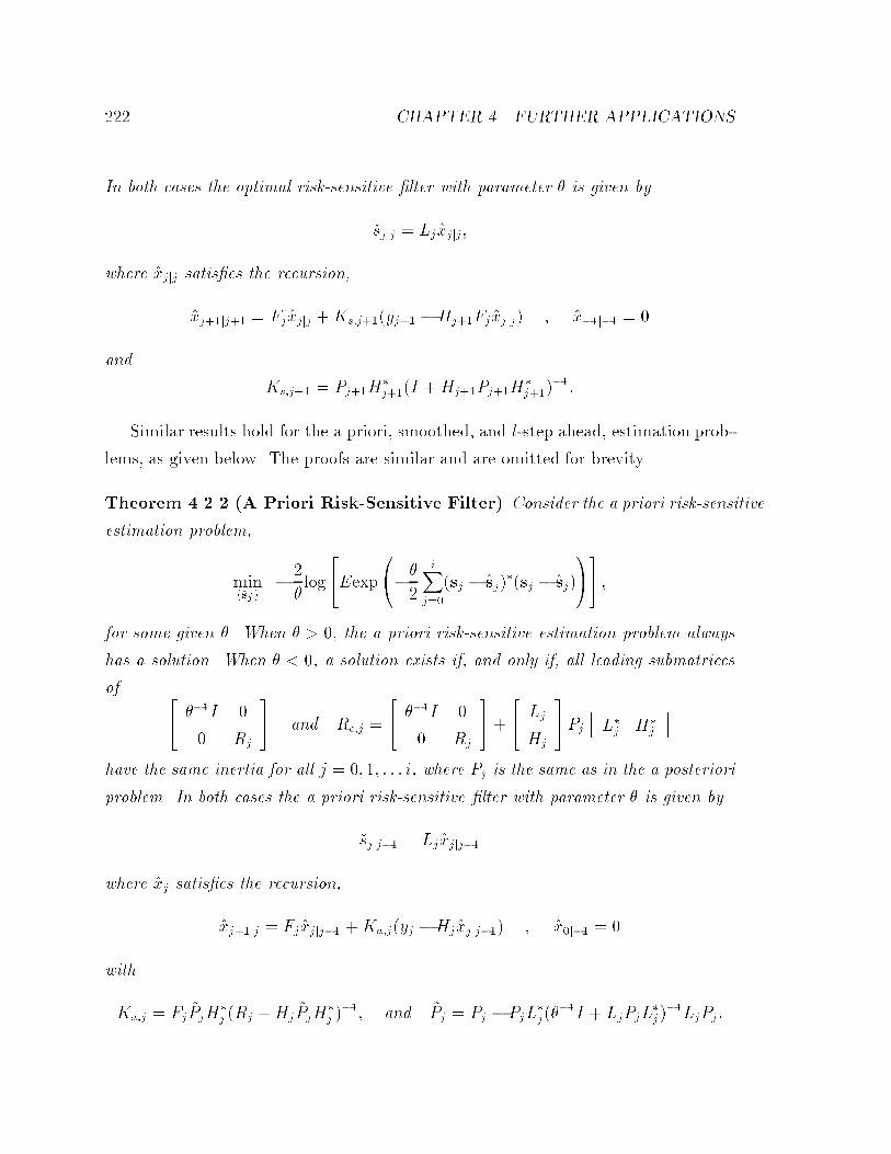
��� CHAPTER �� FURTHER APPLICATIONS
In both cases the optimal risk�sensitive �lter with parameter � is given by
�sjjj � Lj!xjjj�
where !xjjj satis�es the recursion�
!xj��jj�� � Fj!xjjj �Ks�j���yj�� �Hj��Fj!xjjj� � !x��j�� � �
and
Ks�j�� � Pj��H�j���I �Hj��Pj��H
�j���
���
Similar results hold for the a priori� smoothed� and l�step ahead� estimation prob�
lems� as given below� The proofs are similar and are omitted for brevity�
Theorem ����� �A Priori Risk�Sensitive Filter� Consider the a priori risk�sensitive
estimation problem�
minf�sjg
��
�log
��Eexp
����
�
iXj��
�sj � !sj���sj � !sj�
�A� �
for some given �� When � � �� the a priori risk�sensitive estimation problem always
has a solution� When � � �� a solution exists if� and only if� all leading submatrices
of �� ���I �
� Rj
� and Re�j �
�� ���I �
� Rj
��
�� Lj
Hj
�Pj
hL�j H�
j
i
have the same inertia for all j � �� �� � � � i� where Pj is the same as in the a posteriori
problem� In both cases the a priori risk�sensitive �lter with parameter � is given by
�sjjj�� � Lj!xjjj��
where !xj satis�es the recursion�
!xj��jj � Fj!xjjj�� �Ka�j�yj �Hj !xjjj��� � !x�j�� � �
with
Ka�j � Fj#PjH
�j �Rj �Hj
#PjH�j ���� and #Pj � Pj � PjL
�j ��
��I � LjPjL�j ���LjPj �

���� RISK�SENSITIVE ESTIMATION ��
Theorem ���� �Risk�Sensitive Smoother� Consider the smoothed risk�sensitive
estimation problem�
minf�sjjig
��
�log
��Eexp
����
�
iXj��
�sj � !sjji���sj � !sjji�
�A� �
for some given �� When � � �� the smoothed risk�sensitive problem always has a
solution� When � � �� a solution exists if� and only if� the block diagonal matrix
Re � Re�� �Re�� � � � ��Re�i
where
Re�j �
�� Rj �
� ���I
��
�� Hj
Lj
�Pj
hH�
j L�j
i
and Pj is the same as in the a posteriori problem� has �i � ��p positive eigenvalues
and �i� ��q negative eigenvalues� In other words� if� and only if�
In �Re �h�i� ��p � �i� ��q
i�
In both cases the risk�sensitive smoother is the same as the H� smoother�
Theorem ����� �Risk�Sensitive l�Step Predictor� Consider the l�step ahead risk�
sensitive estimation problem�
minf�sjjj�lg
��
�log
��Eexp
����
�
iXj��
�sj � !sjjj�l���sj � !sjjj�l�
�A� �
for some given � and l � �� When � � �� the l�step ahead risk�sensitive problem
always has a solution� When � � �� a solution exists if� and only if� for each j �
�� � � � � i� l�
�i� the two matrices
Re�j �
�� Ip �
� ���Iq
��
�� Hj
Lj
�Pj
hH�
j L�j
iand
�� Ip �
� ���Iq
�
have the same inertia� where Pj is the same as in the a posteriori problem�
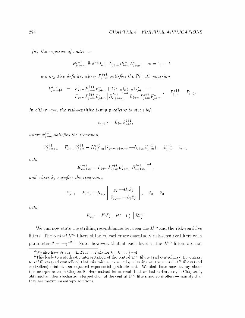
�� CHAPTER �� FURTHER APPLICATIONS
�ii� the sequence of matrices
Rj��e�j�m
�� ���Iq � Lj�mP
j��j�mL
�j�m� m � �� � � � l
are negative de�nite� where P j��j�m satis�es the Riccati recursion
Pj��j�m�� � Fj�mP
j��j�mF
�j�m �Gj�mQj�mG
�j�m�
Fj�mPj��j�mL
�j�m
hR
j��e�j�m
i��Lj�mP
j��j�mF
�j�m
� Pj��j�� � Pj���
In either case� the risk�sensitive l�step predictor is given by
�sj�ljj � Lj�l!xj��j�l �
where !xj��j�m satis�es the recursion�
!xj��j�m�� � Fj�m!xj��j�m �Kj��p�j�m��sj�mjj�m�l � Lj�m!xj��j�m�� !xj��j�� � !xj��
with
Kj��p�j�m � Fj�mP
j��j�mL
�j�m
hR
j��e�j�m
i���
and where !xj satis�es the recursion�
!xj�� � Fj!xj �Kp�j
�� yj �Hj!xj
�sjjj�l � Lj !xj
� � !x� � �x�
with
Kp�j � FjPj
hH�
j L�j
iR��
e�j �
We can now state the striking resemblances between theH� and the risk�sensitive
�lters� The central H� �lters obtained earlier are essentially risk�sensitive �lters with
parameter � � ���� Note� however� that at each level � the H� �lters are not
�We also have skjk�l � LkFk�� � � � F� x� for k � �� � � � � l� ���This leads to a stochastic interpretation of the central H� �lters �and controllers�� In contrast
to H� �lters �and controllers� that minimize an expected quadratic cost� the central H� �lters �andcontrollers� minimize an expected exponential�quadratic cost� We shall have more to say aboutthis interpretation in Chapter �� Here instead let us recall that we had earlier� i�e�� in Chapter ��obtained another stochastic interpretation of the central H� �lters and controllers � namely thatthey are maximum entropy solutions�

���� RISK�SENSITIVE ESTIMATION ���
unique� whereas for each �� the risk�sensitive �lters are unique� Also� the risk�sensitive
�lters generalize to the � � � case� It is also noteworthy that the optimal H� �lter
corresponds to the risk�sensitive �lter with � � ���opt� and that � is that value for
which the minimizing property of Ji breaks down and �i��� becomes in�nite� This
relationship between the optimal H� �lter and the corresponding risk�sensitive �lter
was �rst noted in �GD�� �
����� Risk�Sensitive Control
We should also mention that the risk�sensitive framework can be used to study control
problems� To this end� consider the �possibly time�varying� state�space model�
��� xi�� � Fixi �G��iwi �G��iui
si � Lixi
� � � i � N �������
where fwig is the exogenous input� which is assumed to be a zero�mean Gaussian
stochastic process with variance�
Ewiw�j � Qi�ij� �������
si is the signal we intend to regulate� and ui is the control signal used to in�uence the
dynamics of the system� Moreover� the initial state� x�� is also a zero�mean Gaussian
random variable� independent of the fwig� with variance� ���
Recall that in the H� case� the control signals� fuig were chosen so as to minimize
the expected value of the quadratic cost�
JcN �
NXj��
s�iRcisi �
NXj��
u�iQciui � xN��P
cN��xN��� ������
where the fQci � R
cig and P c
N�� are given positive semide�nite weighting matrices�
In risk�sensitive control� as in risk�sensitive estimation� the objective is to choose
the controls so as to minimize the expected value of an exponential�quadratic cost�
i�e��
minfuig
���
�log
Eexp��
�
�JcN�
��� ������

��� CHAPTER �� FURTHER APPLICATIONS
where � is� once more� referred to as the risk�sensitivity parameter� The remarks pre�
sented at the end of Sec� ���� on risk�neutral� risk�seeking� and risk�averse estimators
apply to the controllers that satisfy ������ in the exact same way� and therefore will
not be repeated here�
Moreover� we should stress that� as was the case in Sec� ���� we can have ei�
ther full information or measurement feedback risk�sensitive controllers� When the
control signals that satisfy ������ are allowed to be causal functions of the states
and exogenous inputs� i�e�� the fxi�wig� then the controller is referred to as a full
information controller� In the measurement feedback case� ui is allowed only to be a
causal function of a certain observation process�
yi � Hixi � vi� �������
where fvig is a zero�mean Gaussian random process such that
E
�����wi
vi
x�
����hw�
j v�j x��
i�
�����Qi�ij � �
� Ri�ij �
� � ��
���� � �������
We shall not go any further into the details of risk�sensitive control here� We just
mention� in passing� that its solution is also amenable to the Krein space techniques
studied so far� Control problems �especially of the H� type� will be studied in
Chapter ��
��� Quadratic Dynamic Games
Game theory is a vast subject with numerous applications in economics and the
social sciences �NM� KT��� Mor�� Col�� � More recently� there has also been
considerable use of game�theoretic ideas and methods in estimation and control �Isa���
Ber�� BH��� KS��� Pon��� BO�� � Even a brief glimpse at this �eld is well beyond
the intentions and scope of this thesis� However� a small subset of game�theoretical
problems� namely the class of quadratic dynamic games� is closely related to the
problems studied in this thesis and lends itself to analysis by the methods that we have

���� QUADRATIC DYNAMIC GAMES ���
used so far�� The reason for this is that quadratic games can be immediately related
to certain inde�nite quadratic forms whose properties can be studied via Krein space
methods� Indeed the �min�max� solutions to such games are found by stationarizing
these quadratic forms and checking for certain minimizing and maximizing conditions�
����� General Remarks
To gain an understanding of quadratic games� consider the quadratic cost function�
J�a� b� �ha� b�
i �� A B
B� C
��� a
b
� � �����
where a � Cn and b � Cm are arbitrary vectors and fA�B�Cg are given matrices
�with A and C Hermitian�� Suppose now that there are two players� say player I and
player II� where player I can choose a and would like to do so to minimize J�a� b��
and where player II would like to maximize J�a� b� through its choice of b� The
central question here �and of game theory in general� is what the optimal strategies
of the players should be�
To this end� suppose that player I has access to player II�s choice of b� Therefore
player I will choose a such that J�a� b� is minimized for that value of b� In this case�
player II�s best strategy will be to choose b such that this minimum value of J�a� b�
is maximized� This then leads to the following �so�called max�min� problem�
maxb
mina
ha� b�
i �� A B
B� C
��� a
b
� � �����
Now clearly the condition for having a �unique� minimum over a is that A � �� Once
this is the case it easy to see that
mina
J�a� b� � b��C �B�A��B�b and argmina
J�a� b� � A��Bb� ����
Now b��C �B�A��B�b will have a maximum over b if� and only if� C �B�A��B � ��
�Incidentally� quadratic dynamic games are the ones that have been most studied in controltheory� and have turned out to be closely related to H� and risk�sensitive control�
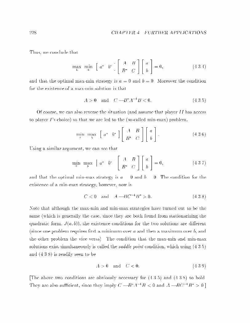
��� CHAPTER �� FURTHER APPLICATIONS
Thus� we conclude that
maxb
mina
ha� b�
i �� A B
B� C
��� a
b
� � �� ����
and that the optimal max�min strategy is a � � and b � �� Moreover the condition
for the existence of a max�min solution is that
A � � and C �B�A��B � �� �����
Of course� we can also reverse the situation �and assume that player II has access
to player I�s choice� so that we are led to the �so�called min�max� problem�
mina
maxb
ha� b�
i �� A B
B� C
��� a
b
� � �����
Using a similar argument� we can see that
mina
maxb
ha� b�
i �� A B
B� C
��� a
b
� � �� �����
and that the optimal min�max strategy is a � � and b � �� The condition for the
existence of a min�max strategy� however� now is
C � � and A�BC��B� � �� �����
Note that although the max�min and min�max strategies have turned out to be the
same �which is generally the case� since they are both found from stationarizing the
quadratic form� J�a� b��� the existence conditions for the two solutions are di�erent
�since one problem requires �rst a minimum over a and then a maximum over b� and
the other problem the vice versa�� The condition that the max�min and min�max
solutions exist simultaneously is called the saddle point condition� which using �����
and ����� is readily seen to be
A � � and C � �� �����
�The above two conditions are obviously necessary for ����� and ����� to hold�
They are also su$cient� since they imply C � B�A��B � � and A� BC��B� � ��
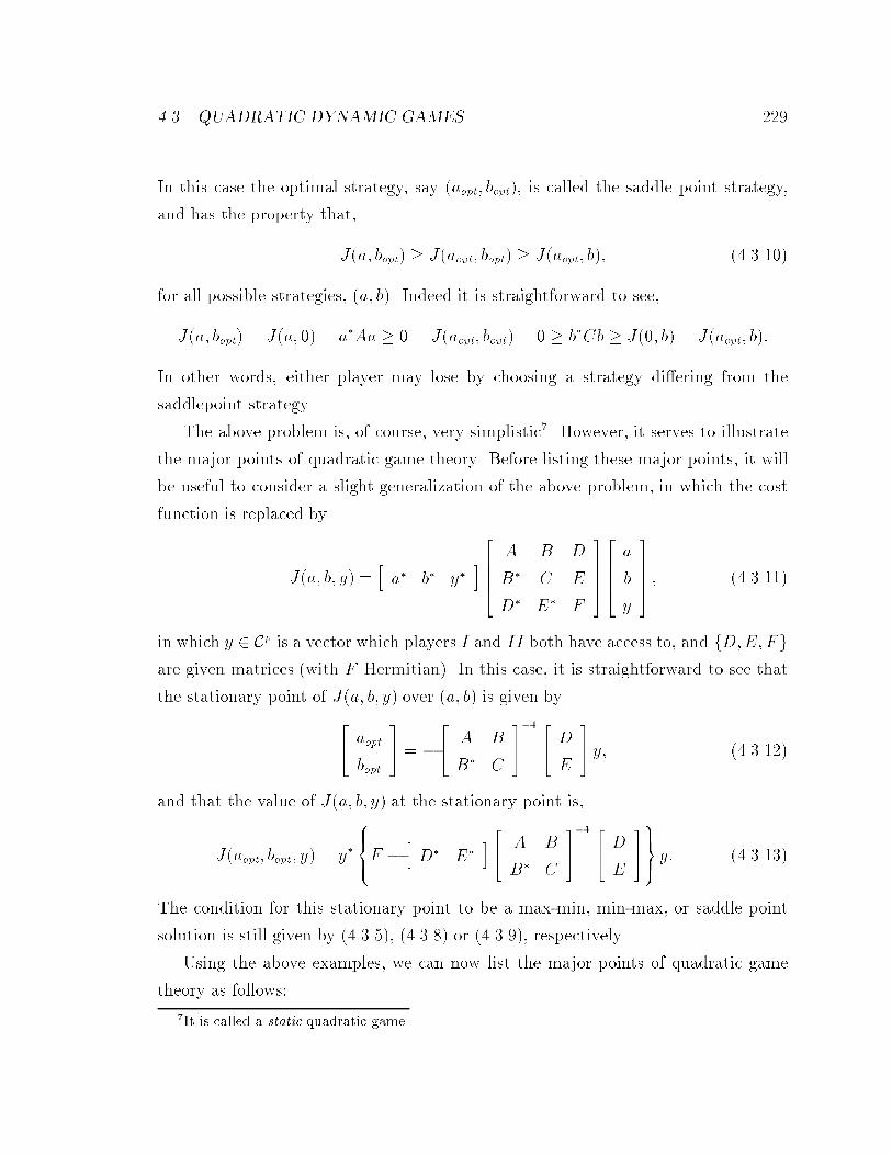
���� QUADRATIC DYNAMIC GAMES ���
In this case the optimal strategy� say �aopt� bopt�� is called the saddle point strategy�
and has the property that�
J�a� bopt� � J�aopt� bopt� � J�aopt� b�� ������
for all possible strategies� �a� b�� Indeed it is straightforward to see�
J�a� bopt� � J�a� �� � a�Aa � � � J�aopt� bopt� � � � b�Cb � J��� b� � J�aopt� b��
In other words� either player may lose by choosing a strategy di�ering from the
saddlepoint strategy�
The above problem is� of course� very simplistic�� However� it serves to illustrate
the major points of quadratic game theory� Before listing these major points� it will
be useful to consider a slight generalization of the above problem� in which the cost
function is replaced by
J�a� b� y� �ha� b� y�
i�����
A B D
B� C E
D� E� F
���������a
b
y
���� � ������
in which y � Cp is a vector which players I and II both have access to� and fD�E�Fg
are given matrices �with F Hermitian�� In this case� it is straightforward to see that
the stationary point of J�a� b� y� over �a� b� is given by
�� aopt
bopt
� � �
�� A B
B� C
��� �� D
E
� y� ������
and that the value of J�a� b� y� at the stationary point is�
J�aopt� bopt� y� � y�
�����F �
hD� E�
i �� A B
B� C
��� �� D
E
������ y� �����
The condition for this stationary point to be a max�min� min�max� or saddle point
solution is still given by ������ ����� or ������ respectively�
Using the above examples� we can now list the major points of quadratic game
theory as follows�
It is called a static quadratic game�
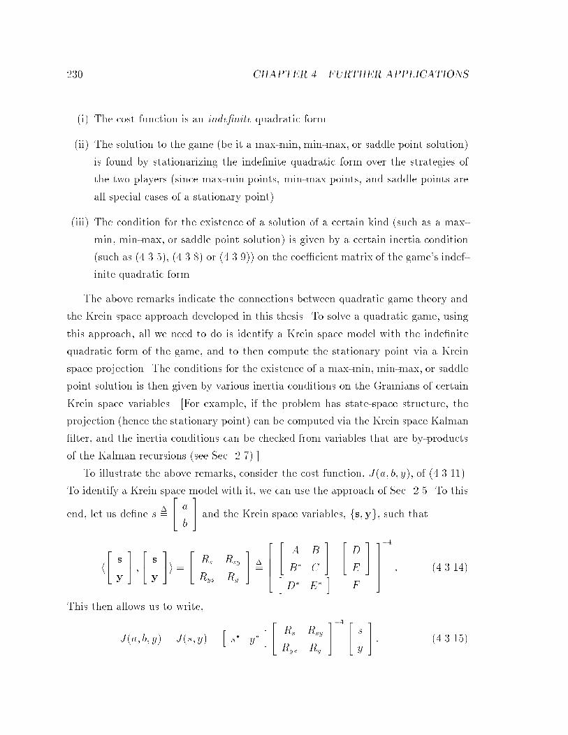
�� CHAPTER �� FURTHER APPLICATIONS
�i� The cost function is an inde�nite quadratic form�
�ii� The solution to the game �be it a max�min� min�max� or saddle point solution�
is found by stationarizing the inde�nite quadratic form over the strategies of
the two players �since max�min points� min�max points� and saddle points are
all special cases of a stationary point��
�iii� The condition for the existence of a solution of a certain kind �such as a max�
min� min�max� or saddle point solution� is given by a certain inertia condition
�such as ������ ����� or ������ on the coe$cient matrix of the game�s indef�
inite quadratic form�
The above remarks indicate the connections between quadratic game theory and
the Krein space approach developed in this thesis� To solve a quadratic game� using
this approach� all we need to do is identify a Krein space model with the inde�nite
quadratic form of the game� and to then compute the stationary point via a Krein
space projection� The conditions for the existence of a max�min� min�max� or saddle
point solution is then given by various inertia conditions on the Gramians of certain
Krein space variables� �For example� if the problem has state�space structure� the
projection �hence the stationary point� can be computed via the Krein space Kalman
�lter� and the inertia conditions can be checked from variables that are by�products
of the Kalman recursions �see Sec� �����
To illustrate the above remarks� consider the cost function� J�a� b� y�� of �������
To identify a Krein space model with it� we can use the approach of Sec� ���� To this
end� let us de�ne s��
�� a
b
� and the Krein space variables� fs�yg� such that
h
�� s
y
� ��� s
y
�i �
�� Rs Rsy
Rys Ry
� ��
������� A B
B� C
�
�� D
E
�
hD� E�
iF
������
� �����
This then allows us to write�
J�a� b� y� � J�s� y� �hs� y�
i �� Rs Rsy
Rys Ry
��� �� s
y
� � ������

���� QUADRATIC DYNAMIC GAMES ��
Using Theorem ������ the stationary point of J�s� y� over s� which we denote by !s� is
given by the Krein space projection of s on L�y�� i�e��
!s � RsyR��y y� ������
Moreover� the conditions for the above stationary point to be a max�min� min�max�
or saddlepoint solution are related to the inertia of the matrix�
�Rs �RsyR��y Rys�
�� �
�� A B
B� C
� � ������
�Recall that methods to determine this inertia have been developed in Secs� ���� and
������
We close this section with one more remark� The quadratic games considered so
far were all static� When the vectors a� b and y are aggregate vectors of some time
series� faig� fbig and fyig� i�e��
a �
���������
a�
a����
aN
��������
� b �
���������
b�
b����
bN
��������
� y �
���������
y�
y����
yN
��������
������
that are dynamically related �say� via a state�space model�� then the game is referred
to as a quadratic dynamic game� In such games� both players �or occasionally one
of the two� have only causal access to the observations� fyig� or to the other player�s
strategy� In other words� the strategy chosen at time i by� say� player I� �which we
recall is just ai� is only allowed to be a function of current and past observations�
fyj� j � ig �and occasionally of current and past strategies of player II� fbj� j � ig��
This causality restriction a�ects both the structure of the optimal strategies and the
actual conditions for the existence of a max�min� min�max or saddle point solution�
Although the solutions in this case are somewhat more complex� they can either be
obtained via a canonical factorization approach of the matrix�
�� A B
B� C
�� �along
The relationship between game theory and inde�nite factorizations were apparently �rst studiedby Yakubovich �Yak��b� and Banker �Ban���

�� CHAPTER �� FURTHER APPLICATIONS
the lines of Secs� ���� and ������ or by performing a recursive stationarization of
the quadratic form J�a� b� y� �along the lines of Sec� ����� In summary� there is no
essential di�erence between the methods for solving dynamic games with a causality
restriction and the methods for �nding causal estimators and controllers that have
been studied so far�
����� Speci�c Examples
We now very brie�y turn to some special cases of the general quadratic games de�
scribed above� The examples we consider are in the contexts of �state�space� estima�
tion and control and are intimately related to the H� and risk�sensitive formulations
studied earlier� In essence� we shall see that the central H� �lters and controllers�
and the risk�sensitive �lters and controllers� can be considered as the solutions to
certain quadratic dynamic games�
Estimation Problems
Consider the standard state�space model
���������xi�� � Fixi �Giui� x�
yi � Hixi � vi
si � Lixi
� � i � N ������
where� as usual� the initial condition x�� and the disturbances� fui� vig� are unknown�
fyig is the observations sequence� and fsig is the signal we intend to estimate �using
the observations�� In the game�theoretic approach to estimation� the unknown distur�
bances fx�� fu�vigNi��g are considered to be an adversary whose objective is to disrupt
our attempt at estimating the fsig� To be more speci�c� consider the a posteriori
�ltering problem where the estimates are given by �siji � Ff�i�y�� � � � � yi�� with Ff���
being the estimation strategy that must be determined� Now one measure of how
well our estimation scheme is performing is the estimation error energy�
NXi��
�si � �siji���si � �siji�� ������

���� QUADRATIC DYNAMIC GAMES �
Roughly speaking� our objective is to choose the estimator� Ff ��� so as to minimize
the estimation error energy� whereas nature�s �our adversary�s� objective is to choose
the disturbances so as to maximize it� To put the situation on an equal footing� one
must include a penalty on the choice of large disturbances �otherwise nature could
make the estimation error arbitrarily large by choosing arbitrarily large disturbances��
This is achieved by adding a negative de�nite quadratic term to the above cost that
penalizes large disturbances� Thus we are led to the following cost function�
JN �NXi��
�si � �siji���si � �siji�� �
�x���
��� x� �
NXi��
u�iQ��i ui �
NXi��
v�iR��i vi
�� ������
where ��� Qi and Ri are given positive de�nite weighting matrices� and where
is a scalar that determines the respective contributions of the estimation error and
disturbance energies to the cost function JN �
The game�theoretic estimation problem can be thus formulated as follows�
minf�sijig
maxx��fuig�fvig
NXi��
�si � �siji���si � �siji�� �
�x���
��� x� �
NXi��
u�iQ��i ui �
NXi��
v�iR��i vi
��
������
where �siji � Ff�i�y�� � � � � yi� and the fx�� fuig� fvig� fyig� fsigg are related via the
state�space model �������
Now the quadratic form� JN � is an inde�nite quadratic form of the standard type
that has been studied since Chapter �� Therefore we can readily use the Krein space
Kalman �lter to compute the stationary point of JN and to check whether the sta�
tionary point has the desired �maximum over fx�� fuig� fvigg� minimum over f�sijig�
properties �via certain inertia conditions obtained from the Kalman �lter recursions��
Indeed further inspection of JN reveals that� apart from a minus sign� it is the exact
same inde�nite quadratic form that was studied in the H� and risk�sensitive a pos�
teriori estimation problems� Following through with the arguments presented there�
�which we will not repeat here� shows that the central H� and risk�sensitive a poste�
riori �lters are� in fact� given by the solution to the game �������� Similar statements
hold for the a priori� smoothed� and l�step ahead central H� and risk�sensitive �lters
as well��This observation is the whole premise of the game�theoretic approach to H� estimation and
control �see e�g�� �BB��� LAKG�����

� CHAPTER �� FURTHER APPLICATIONS
The above remarks conclude our brief study of game�theoretic estimation and we
now turn our attention to control�
Control Problems
Consider the state�space model�
��� xi�� � Fixi �G��iwi �G��iui� x�
si � Lixi� � i � N �����
where fwig is the exogenous input� fsig is the signal we want to regulate� and fuig is
the control input� In the full information problem� the control signal ui is allowed to
be a function of the initial state� x�� and of the current and past exogenous inputs�
fwj� j � ig� In the measurement feedback problem� all we have access to is the
measurement signal�
yi � Hixi � vi� �����
where fvig is an �unknown� measurement disturbance� and therefore the control signal
ui is only allowed to be a function of current and past observations� fyj� j � ig� In
either case� the control objective is to minimize the quadratic cost�
NXj��
s�iRcisi �
NXj��
u�iQciui � xN��P
cN��xN��� ������
In the game�theoretic approach to control the disturbances x�� fwig� and in the
case of measurement feedback control� fvig� are considered to be adversaries that
choose to maximize the above cost� As in estimation� to level the playing �eld� we
must penalize the choice of large values of disturbances on the part of nature �our
opponent�� This is achieved by adding a negative de�nite quadratic term to the above
cost that penalizes large disturbances� We are thus led to the following cost functions�
for the full information problem�
J cN �
NXj��
s�iRcisi �
NXj��
u�iQciui � xN��P
cN��xN�� � �
�x���
��� x� �
NXi��
u�iQ��i ui�
��
������

���� QUADRATIC DYNAMIC GAMES ��
and for the measurement feedback problem�
J cN �
NXj��
s�iRcisi�
NXj��
u�iQciui�xN��P
cN��xN���
�
�x���
��� x� �
NXi��
u�iQ��i ui �
NXi��
v�iR��i vi
��
������
where ��� Qi and Ri are given positive de�nite weighting matrices� and where is a
scalar that determines the respective contributions of the original quadratic cost and
disturbance energies to the cost function J cN �
The game�theoretic estimation problem can be thus formulated as follows� for the
full information problem�
minfuig
maxx��fuig
J cN � ������
where ui � Fi�x�� w�� � � � � wi�� JcN is given by ������� and the fsig� and fx�� fwi� uigg
are related via ������ for the measurement feedback problem�
minfuig
maxx��fuig�fvig
J cN � ������
where ui � Fi�y�� � � � � yi�� J cN is given by ������� and the fsi� yig and fx�� fwi� ui� vigg
are related via ����� and ������
The quadratic form� J cN � is an inde�nite quadratic form� but not of the type that
has been studied since Chapter �� In Chapter � we shall show that this quadratic
form can be motivated� and introduced� via the concept of a dual basis� and that its
stationary point can be obtained by certain projections� not in the original spaces� but
in the resulting dual spaces� �This is yet another manifestation of the duality between
estimation and �full information� control� that we �rst noted in Sec� ������ In fact� the
aforementioned duality is geometric while the one presented in Sec� ����� was purely
algebraic� We shall not give the details of how to compute these stationary points
�or how to verify the min�max or saddle point conditions� here� since that topic will
be studied in length in Chapter �� Instead� we close this section by remarking that
the inde�nite quadratic form J cN is exactly the same �apart from a minus sign� as
the inde�nite quadratic form that is obtained from H� and risk�sensitive control� In
particular� it turns out that the full information and measurement feedback H� and
risk�sensitive controllers coincide with the solutions to the quadratic dynamic games
������ and ������� respectively�

�� CHAPTER �� FURTHER APPLICATIONS
��� Finite Memory Adaptive Filtering
We now consider an application of the Krein space Kalman �lter to the problem of
�nite memory �or sliding window� adaptive �ltering��� It has been recently shown
�SK�b that a uni�ed derivation of adaptive �ltering algorithms� and their corre�
sponding fast versions� can be obtained by properly recasting the adaptive problem
into a standard state�space estimation problem� We now verify that if we further
allow the elements of the state�space model to belong to a Krein space� then the so�
called sliding window or �nite�memory problem can also be handled within the same
framework� In fact� this framework also allows us to easily consider more general
sliding patterns with windows of varying lengths� as explained ahead� Moreover� we
shall obtain a physical interpretation of innovations with negative Gramian� and see
that it corresponds to the loss of information�
����� The Standard Problem
The �nite memory adaptive �ltering problem can be formulated as follows� given the
input�output pairs fhj� djg where hj � C��n is a known input vector and dj � C is
a known output scalar� recursively determine estimates of an unknown weight vector
w � Cn� such that the scalar quadratic form
Ji�w� di�li��� � � � � di� hi�li��� � � � � hi� � w����� w�
iXj�i�li�i
�dj�hjw���dj�hjw�� �����
with �� � � a given weighting matrix and the flig given �time�varying� window
lengths� is minimized for each i�
Since Ji is a function of the pairs fhj� djgij�i�li�i� at each time instant i� we are
interested in determining the estimate of w using only the data given over an interval
of length li� The quantity li � � is therefore referred to as the length �or memory� of
the sliding window�
Note that we allow for a time�variant window length� To clarify this point� consider
the example of Fig� �� where at time i we have a window of length li � l� At the next
��Refer back to Sec� ����� for a brief introduction to adaptive �ltering� The topic will be furtherstudied in Chapters � and ���

���� FINITE MEMORY ADAPTIVE FILTERING ��
( )
( ) )
( ) ) )
))
) )
)
hi
di
h d
h dii
(h d
(h d
i+1 i+1
i+1i+1(h d
i+2 i+2
(h di-l i-l
(h di-l+1 i-l+1
(h d
(h d (h di-l i-l i-l+1 i-l+1
i-l+1 i-l+1
i i
Length l = l
+1
i
i+1l = lLength
Length l = l+1i+2
Time i+2
Time i+1
Time i
Figure ��� Sliding window with varying window length�
time instant we add the data point fhi��� di��g� so that the window length changes
to li�� � l � �� At time i� � we add the data point fhi��� di��g and drop the data
point fhi�l� di�lg so that the window length remains li�� � l��� In a similar fashion�
more general sliding window patterns can be considered as well�
To recast expression ����� into the usual quadratic form considered in this chap�
ter� the lower index of the summation term needs to start at the �xed time �� For
this purpose� we rewrite Ji as follows
Ji�w� di�li��� � � � � di� hi�li��� � � � � hi� � w����� w �
iXj�i�li��
�dj � hjw���dj � hjw�
�i�liXj��
�dj � hjw���dj � hjw��
i�liXj��
�dj � hjw���dj � hjw� �����
where we have added and subtracted identical terms� We now invoke a change of
variables and substitute the time index i by another time index k that allows us to
replace Ji by a Jk� The new index k has the property whenever a new data point
is added �i�e� � i is incremented� then k is incremented� However� whenever a data
point is discarded from the window� k is incremented as well� Thus if at time i the
length of the window is li� then the index k will run from � to �i� li � � �since there

�� CHAPTER �� FURTHER APPLICATIONS
will have been i data points added and i� li � � data points removed�� To be more
speci�c� the change of variables is as follows�
�a� At each time i� since the data point fhi� dig is added� we increment the index k
and de�ne
dk � di� hk � hi and Rk � �� ����
�b� If at time i the data point fhi�li� di�lig is removed� we increment the index k
once more and de�ne
dk � di�li� hk � hi�li and Rk � ��� ����
With this convention we may write the quadratic form
Ji�w� di�li��� � � � � di� hi�li��� � � � � hi��
as
Ji � Jk�w� d�� � � � � dk� h�� � � � � hk� � w����� w �
kXj��
� dj � hjw��� dj � hjw�� �����
which is of the form that we have been considering in this thesis since Chapter ��
Note that the quadratic form Jk�w� d�� � � � � dk� h�� � � � � hk� is inde�nite� since whenever
a data point is dropped we have Rk � ��� We can therefore use Krein space methods
to solve the problem�
Using the same approach that we have used so far� we now construct the partially
equivalent state�space model to the inde�nite quadratic form Jk� Thus��� xj�� � xj� x� � w � � j � k
dj � hjxk � vk
�����
with � � �� Qj � �� Sj � � and Rj as in ���� and �����
We can now state the following result�
Theorem ����� �Finite Memory Adaptive Filter� The �nite memory adaptive
�lter is given by the following recursions�

���� FINITE MEMORY ADAPTIVE FILTERING ��
�a� For updating� the data point fhi� dig at time i we have
!wji�i�li��� !wji���i�li��
�Kp�k�di � hi !wji���i�li��� �����
where !wji�j is the estimate when the sliding window encompasses all the data
from time j to time i� and
Kp�k � Pkh�iR
��e�k � Re�k � � � hiPkh
�i �����
and where Pk satis�es the recursion
Pk�� � Pk �Kp�kRe�kK�p�k� P� � ��� �����
�b� For downdating� the data point fhi�li� di�lig at time i we have
!wji�i�li�� � !wji�i�li �Kp�k�di�li � hi�li !wji�i�li� ������
where
Kp�k � Pkh�i�li
R��e�k � Re�k � �� � hi�liPkh
�i�li
������
and Pk satis�es the recursion
Pk�� � Pk �Kp�kRe�kK�p�k� ������
Moreover� the above solutions for !wji�j always correspond to a minimum� and in par�
ticular
Re�k � � � hiPkh�i � �� �����
when we are updating� and
Re�k � �� � hi�liPkh�i�li
� �� �����
when we are downdating�
Proof The solutions given by �a� and �b� in the above Theorem are simply the
Krein space Kalman �lter recursions for the state�space model ����� which we know

�� CHAPTER �� FURTHER APPLICATIONS
computes the stationary point of Jk over w� However� this stationary point is always
a minimum since� Jkw�
��Ji
w�� ���
� �iX
j�i�li��
h�jhj � ��
�recall that ���� � ���
Using Lemma ����� having a minimum means that Re�k and Rk have the same
inertia for all k� Thus the statements ����� and ����� readily follow�
The fact that whenever we drop data we have Re�k � � has an interesting inter�
pretation� Consider the equation
Pk�� � Pk �Kp�kRe�kKp�k
If we drop data at step k we would expect Pk�� to get larger �more positive�de�nite�
than Pk� This can only happen if Re�k � �� Thus� we may infer that innovations with
negative Gramian correspond to a loss of information�
The above discussion puts the problem of �nite memory adaptive �ltering into the
same state�space estimation framework as conventional adaptive �ltering techniques
�see �SK�b �� Therefore the various algorithmic extensions discussed there may be
applied to �nite memory problems� albeit that we now need to consider a Krein space�
We shall not give the details here� but shall just mention that when the elements of
the input vectors fhig form a time sequence� viz��
hi �hui ui�� � � � ui�n��
i�
and when the window length is constant� i�e� � li � l� then the state�space model
����� is periodic with period T � �� and we may speed up the the estimation
algorithm by a so�called Chandrasekhar�type recursion� Similar results� obtained via
a di�erent approach� have been reported in �Hou�� �
��� Conclusion
In this chapter we studied the problems of risk�sensitive estimation and control�
quadratic game theory� and �nite memory adaptive �ltering� using the framework

���� CONCLUSION ��
of linear estimation in Krein spaces that was developed in Chapter �� The theme
that unites all these problems is that they can be related� albeit in an indirect fash�
ion� to certain inde�nite quadratic forms� We anticipate that there should be other
problems that are amenable to this approach� and mention� in passing� an interesting
application to recursive algorithms for �suboptimal� total least�squares problems that
has been given in �SHK��a �
Chapter �
Square�Root Arrays and
Chandrasekhar Recursions
Using the observation that H� �ltering coincides with Kalman �ltering in Krein
space� in this chapter we develop square�root arrays and Chandrasekhar recursions for
H� �ltering problems� These are the generalizations of the conventional square�root
arrays and Chandrasekhar recursions to the Krein space setting� The H� square�root
algorithms involve propagating the inde�nite square�root of the quantities of interest
and have the property that the appropriate inertia of these quantities is preserved�
For systems that are constant� or whose time�variation is structured in a certain
way� the Chandrasekhar recursions allow a reduction in the computational e�ort per
iteration from O�n�� to O�n��� where n is the number of states� The H� square�root
and Chandrasekhar recursions both have the interesting feature that one does not
need to explicitly check for the positivity conditions required of the H� �lters� These
conditions are built into the algorithms themselves so that an H� estimator of the
desired level exists if� and only if� the algorithms can be executed� The results of
this chapter were �rst reported in HSK�c���
�

���� INTRODUCTION ��
��� Introduction
In Chapter we presented a self�contained theory for linear estimation in Krein
spaces with the objective of unifying the H�� H�� risk�sensitive and game�theoretic
approaches to estimation and control� There we claimed that the major bonus of this
approach is that� apart from rather more transparent derivations of existing results
�as done in Chapters � and ��� it shows a way to apply to the H� �and these other�
settings many of the results developed for Kalman �ltering and LQG control over
the last three decades� In this chapter we intend to support this claim by showing
how the Krein space approach can be used to naturally extend the �numerically supe�
rior� square�root and �fast� Chandrasekhar array recursions of conventional Kalman
�ltering to H� �ltering�
The �so�called� square�root array algorithms were devised in the late ����s DM��
KBS��� Har� �� and� for several reasons� are currently more often used to implement
the conventional Kalman �lter� These algorithms are closely related to the �so�called�
QR method for solving systems of linear equations BG��� GL�� HJ�� Str��� and
have the properties of better conditioning� reduced dynamical range� and the use of
orthogonal transformations� which typically leads to stabler algorithms�
Furthermore for constant systems� or in fact for systems where the time�variation
is structured in a certain way� the Riccati recursions and the square�root recursions�
both of which take O�n�� elementary computations ��ops� per iteration �where n is
the dimension of the state�space�� can be replaced by more e�cient recursions� which
require only O�n�� �ops per iteration Kai� � MSK��� SK�a�� These algorithms are
analogous to certain equations invented in ������ by the astrophysicists Ambartsum�
ian Amb��� and Chandrasekhar Cha��� �hence the name Chandrasekhar recursions��
are also closely related to the concept of displacement structure KKM�� Say ��
One immediate fall�out of our observation thatH� �ltering coincides with Kalman
�ltering in Krein space is that it allows us to generalize these square�root arrays
and Chandrasekhar recursions to the H� setting� Both these algorithms involve
propagating �inde�nite� square�roots of the quantities of interest and guarantee that
the proper inertia of these quantities is preserved� Furthermore� the condition required
��CHAPTER �� SQUARE�ROOTARRAYSANDCHANDRASEKHARRECURSIONS
for the existence of the H� �lters is built into the algorithms � if the algorithms can
be carried out� then an H� �lter of the desired level exists� and if they cannot be
executed then such H� �lters do not exist� This can be a signi�cant simpli�cation
of the existing algorithms�
The remainder of the chapter is organized as follows�
The conventional square�root array algorithms are introduced in Sec� �� along
with some of their properties� In Sec� ��� we begin the development of the H�
square�root array algorithms and mention why they are natural extensions of their
conventional counterparts� We initially encounter some di�culties in generalizing
these arrays to the Krein space setting� and in order to alleviate them we then intro�
duce the concept of inde�nite square�roots� and study the inertia properties of the
Gramian matrices in the H� �ltering problem in some detail� These inertia proper�
ties are related to the triangularization of matrices via J �unitary transformations and
will be crucial for the development of the H� square�root array and Chandrasekhar
recursions� Finally� the general form of the H� a posteriori and a priori �lters are
given in Sec� ����� and the central �lters in Sec� ���� �
The conventional �fast� Chandrasekhar recursions� along with several of their
properties� is given in Sec� ���� Sec� ����� extends these recursions to the H�
setting� and Sec� ���� gives the corresponding central H� �lters�
In closing this introduction we note that there are many variations to the con�
ventional square�root arrays and Chandrasekhar recursions� of which only a few have
been considered here� However� the approach adopted here is of su�cient generality
that it should allow a reader to extend any other variation of these algorithms to the
H� setting�
A brief remark on the notation used in this chapter� To avoid confusion between
the various gain vectors used in this chapter� we shall employ the following convention�
Kp�i will denote the gain vector in the usual Krein space �or Hilbert space� Kalman
�lter� Kf�i the gain vector in the �ltered form of the Krein space Kalman �lter� and
Ks�i and Ka�i will denote the gain vectors in the H� a posteriori and a priori �lters�
respectively�
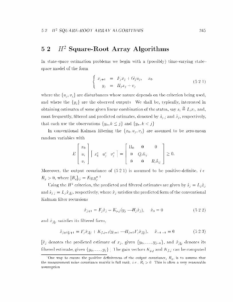
���� H� SQUARE�ROOT ARRAY ALGORITHMS ��
��� H Square�Root Array Algorithms
In state�space estimation problems we begin with a �possibly� time�varying state�
space model of the form���xj�� � Fjxj �Gjuj� x�
yj � Hjxj � vj��� ���
where the fuj� vjg are disturbances whose nature depends on the criterion being used�
and where the fyjg are the observed outputs� We shall be� typically� interested in
obtaining estimates of some given linear combination of the states� say si�� Lixi� and�
most frequently� �ltered and predicted estimates� denoted by �sjjj and �sj� respectively�
that each use the observations fyk� k � jg and fyk� k � jg�
In conventional Kalman �ltering the fx�� uj� vjg are assumed to be zero�mean
random variables with
E
�����x�
ui
vi
����hx�� u�j v�j
i�
������� � �
� Qi�ij
� � Ri�ij
���� � ��
Moreover� the output covariance of ��� ��� is assumed to be positive�de�nite� i�e�
Ry � �� where Ry�ij � Eyiy�j ��
Using the H� criterion� the predicted and �ltered estimates are given by �sj � Lj�xj
and �sjjj � Lj �xjjj� respectively� where �xj satis�es the predicted form of the conventional
Kalman �lter recursions
�xj�� � Fj�xj �Kp�j�yj �Hj �xj�� �x� � � ��� � �
and �xjjj satis�es its �ltered form�
�xj��jj�� � Fj�xjjj �Kf�j���yj�� �Hj��Fj�xjjj�� �x��j�� � � ��� ���
�xj denotes the predicted estimate of xj� given fy�� � � � � yj��g� and �xjjj denotes its
�ltered estimate� given fy�� � � � � yjg�� The gain vectors Kp�j and Kf�j can be computed
�One way to ensure the positive de�niteness of the output covariance� Ry� is to assume thatthe measurement noise covariance matrix is full rank� i�e�� Ri � �� This is often a very reasonableassumption�

��CHAPTER �� SQUARE�ROOTARRAYSANDCHANDRASEKHARRECURSIONS
in several ways� The most common method uses a certain Riccati recursion� viz��
Kf�j�� � Pj��Hj��R��e�j�� � Kp�j � FjKf�j�� � Re�j � Rj �HjPjH
�j ��� ���
where Pj satis�es the Riccati recursion�
Pj�� � FjPjF�j �GjQjG
�j �Kp�jRe�jK
�p�j� P� � ��� ��� ���
The invertibility of the Re�j is guaranteed by the positivity assumption on Ry��
The matrix Pj appearing in this Riccati recursion has the physical meaning of
being the variance of the state prediction error� �xj � xj � �xj� and therefore has to be
positive �semi�de�nite� Round�o� errors can cause a loss of positive�de�niteness� thus
throwing all the obtained results into doubt� For this� and other reasons �reduced
dynamic range� better conditioning� stabler algorithms� etc�� attention has moved
in the Kalman �ltering community to the so�called square�root array �or factorized�
estimation algorithms DM�� KBS��� that propagate square�root factors of Pj � i�e�
a matrix� P���j say� with positive diagonal entries� and such that
Pj � P���j �P ���
j �� � P���j P
���j �
Square roots can be similarly de�ned for the system covariances fQj� Rjg� Then it is
in fact not hard to show the following�
Find any orthogonal transformation� say �j�� that triangularizes the pre�array
shown below �� R
���i HjP
���j �
� FjP���j GjQ
���j
��j �
�� X � �
Y Z �
� � ��� ���
The resulting post�array entries can be checked� by taking squares and using the
orthogonality of �j � to obey
XX� � Rj �HjPjH�j � Re�j
Y X� � FjPjH�j
ZZ� � FjPjF�j �GjQjG
�j � Y Y �
� FjPjF�j �GjQjG
�j � Y X��XX����XY �
�By an orthogonal transformation� �� we mean one for which� ��� � ��� � I�

���� H� SQUARE�ROOT ARRAY ALGORITHMS ��
� FjPjF�j �GjQjG
�j � FjPjH
�jR
��e�jHjPjF
�j
� Pj���
Therefore we can identify
Z � P���j�� � X � R
���e�j ��� ���
and also
Y � FjPjH�jR
����e�j � Kp�jR
���e�j � ��� ���
Thus the square�root algorithm not only propagates the square�roots of the Riccati
variable� Pj � but also gives us quantities useful for the state estimation recursion
�xj�� � Fj�xj �Kp�jR����e�j �yj �Hj �xj��
The unitary transformation �j is highly nonunique and can be computed in many
ways� the simplest ones being to construct it as a sequence of elementary �Givens
or plane� rotations nulling one entry at a time in the pre�array� or as a sequence of
elementary �Householder� re�ections nulling out a block of entries in each row� We
refer to Hou��� GL�� Str�� for more details�� The numerical advantages of the
square�root transformations arise from the length preserving properties of unitary
transformations� and from the fact that the dynamic range of the entries in P���j
is roughly the square�root of the dynamic range of those in Pj � Moreover� regular
computational �systolic� arrays can be designed to implement sequences of elementary
unitary transformations ML ��
A �nal result will be useful before we summarize the above discussion in a theorem�
Any unitary transformation �j that triangularizes the pre�array in ��� ��� also gives
the� readily checked� identity�
h�R
����j yj P
����j �xj �
i�j �
hR����e�j ej P
����j�� �xj�� �
i��� ��
where � denotes an entry whose exact form is not relevant at the moment�
We can summarize the above discussion as follows�
�The above square�root method is closely related to the QR factorization method for solvingsystems of linear equations�

��CHAPTER �� SQUARE�ROOTARRAYSANDCHANDRASEKHARRECURSIONS
Algorithm ����� �Conventional Square�Root Algorithm� The gain vectorKp�j
necessary to obtain the state estimates in the conventional Kalman �lter
�xj�� � Fj�xj �Kp�j�yj �Hj�xj�� �x� � ��
can be updated as follows�� R
���j HjP
���j �
� FjP���j GjQ
���j
��j �
�� R
���e�j � �
Kp�jR���e�j P
���j�� �
� � ��� ����
where �j is any unitary matrix that triangularizes the above pre�array� The algorithm
is initialized with P� � ���
Note that the quantities necessary to update the square�root array� and to calcu�
late the state estimates� may all be found from the triangularized post�array�
It will also be useful to quote the �ltered form of the square�root array algorithm�
that can be veri�ed in a fashion similar to what was done above�
Algorithm ����� �Conventional Square�Root Algorithm � Filtered Form� The
gain vector Kf�j necessary to obtain the state estimates in the �ltered form of the con�
ventional Kalman �lter
�xj��jj�� � Fj�xjjj �Kf�j���yj�� �Hj��Fj�xjjj�� �x��j�� � ��
can be updated as follows�� R
���j HjP
���j
� P���j
�����
j �
�� R
���e�j �
Kf�jR���e�j P
���jjj
� � ��� ����
hFjP
���jjj GjQ
���j
i����
j �hP���j�� �
i��� �� �
where ����j and ����
j are any unitary matrices that triangularize the above pre�arrays�
The algorithm is initialized with P� � ���
��� H� Square�Root Array Algorithms
We now turn our attention to H� �ltering� Our goal here is to investigate whether
it is possible to construct square�root array implementations of H� �lters� similar to
what was done in the aforementioned H� case�

���� H� SQUARE�ROOT ARRAY ALGORITHMS �
����� The General Case
Recall the parametrization of all possible H� a posteriori �lters� sjjj � Ff�j�y�� � � � yj��
as given by Lemma ������ There we saw that all such sjjj are given by any choices
that render
kXj�
�� yj �Hj �xj
sjjj � Lj �xj
��
R��e�j
�� yj �Hj �xj
sjjj � Lj�xj
� � �� � � k � i �������
where �xj satis�es the recursion�
�xj�� � Fj�xj �Kp�j
�� yj �Hj �xj
sjjj � Lj �xj
� � �x� � � ����� �
with
Kp�j � FjPj
hH�
j L�j
iR��e�j and Re�j �
�� Ip �
� ���Iq
��
�� Hj
Lj
�Pj
hH�
j L�j
i
�������
and
Pj�� � FjPjF�j �GjQjG
�j �Kp�jRe�jK
�p�j� P� � ��� �������
As repeatedly mentioned earlier� the above solution looks very much like the con�
ventional Kalman �lter� The essential di�erence is in the Riccati recursion where we
now have inde�nite covariance matrices �such as Re�i�� Nonetheless� let us persist to
see whether we can come up with a square�root implementation of the H� Riccati
recursion ��������
To this end� recall the conventional square�root array algorithm of Sec� �� �
�� R
���j HjP
���j �
� FjP���j GjQ
���j
��j �
�� R
���e�j � �
Kp�jR���e�j P
���j�� �
� � �������
where P���j P
���j � Pj � Q
���j Q
���j � Qj� R
���j R
���j � Rj� and R
���e�j R
���e�j � Re�j �
Using our earlier observation that H� �ltering is just Kalman �ltering in Krein
space� allows us to speculate that needs to be done is to come up with a Krein space
generalization of the above square�root array algorithm� This is the approach that
we shall take here�

��CHAPTER �� SQUARE�ROOTARRAYSANDCHANDRASEKHARRECURSIONS
The �rst problem that occurs if one wants to extend the square�root array algo�
rithm to the Krein space setting �of which the H� �ltering problem is a special case�
is that the matrices Ri� Qi� Pi and Re�i are in general inde�nite and square�roots may
not exist� To alleviate this problem we need the notion of an inde�nite square�root�
as de�ned below�
Denition ���� �Indenite Square�Roots� Suppose A is an arbitrary Hermitian
matrix� A��� will be called an inde�nite square�root of A if� and only� if
A � A���SA���
where S is a signature matrix �i�e� a diagonal matrix with diagonal elements either
�� or ����
However� in the Krein space case Ri� Qi� Pi and Re�i may all have arbitrary inertia�
i�e�
Ri � R���i S
���i R
���i � Qi � Q
���i S
���i Q
���i � Pi � P
���i S
���i P
���i � Re�i � R
���e�i S
��i R
���e�i
for arbitrary signature matrices S�k�i � k � �� � �� �� It is thus not obvious how to
incorporate all these di�erent time�varying signature matrices into a square�root array
algorithm of the type �������� Although this can be done in the general case� by either
introducing non�Hermitian factorizations of the Gramians� or by keeping track of the
inertia� we shall not pursue these lines of thought here� The reason is that� as it turns
out� in the H� problems that we have been studying� the Gramians satisfy certain
inertia properties that allow us to extend the algorithm of ������� in a very natural
way�
Indeed when a solution to the H� �ltering problem exists� we know that Pi �
�� and that Re�i and Ri have the same inertia �see e�g�� Lemmas ���� and ������
Moreover� Qi � Im � � and Ri �
�� Ip �
� ���Iq
� have constant inertia �and thus so
does Re�i� so that we may write�
Ri � R���i JR
���i � Qi � Q
���i Q
���i � Pi � P
���i P
���i � Re�i � R
���e�i JR
���e�i �������

���� H� SQUARE�ROOT ARRAY ALGORITHMS ��
with
R���i �
�� Ip �
� �Iq
� and J �
�� Ip �
� �Iq
� � �������
This suggests that in the H� �ltering problem� the prearray in ������� should be
replaced by� �����
�� Ip �
� �Iq
�
�� Hj
Lj
�P ���
j �
� FjP���j Gj
���� � �������
Recall that in H� estimation Hj is replaced by
�� Hj
Lj
��� Now in the H� case the
prearray in ������� was triangularized by a unitary transformation �or simply by a
rotation�� Since the H� estimation problem can be formulated in a Hilbert space�
whereas the H� estimation problem is most naturally formulated in a Krein space�
it seems plausible that we should attempt to triangularize �������� not by an ordinary
rotation� but by a hyperbolic rotation� To be more speci�c� we need to use a J �unitary
transformation� as de�ned below�
Denition ���� �J�unitary Matrices� For any signature matrix� J � �a diagonal
matrix with �� and �� diagonal elements� the matrix � will be called J�unitary if
�J�� � J� ������
Recall that unitary transformations �or ordinary rotations� preserve the length �or
ordinary norm� of vectors� J �unitary transformations� on the other hand� preserve
the �inde�nite� J �norm of vectors� Indeed� if b � a�� with � J �unitary� then
bJb� � a�J��a� � aJa��
The above discussions suggest that we should attempt to triangularize ������� via
a J �unitary transformation� where��������
�� Ip �
� �Iq
�
In
Im
�������� ��������

� CHAPTER �� SQUARE�ROOTARRAYSANDCHANDRASEKHARRECURSIONS
Now it is well known that it is always possible to triangularize arrays using unitary
transformations� But is this also true of J �unitary transformations! To see if this is
the case� consider a much simpler example where we are given the �two�element� row
vector ha b
i�
and are asked to hyperbolically rotate it to that the resulting vector lies along the
direction of the x�axis� For the time being� assume that such a transformation can
be found� Then we can write�
ha b
i� �
hc �
i� ��������
where
�J�� � J and J �
�� �
��
� � ������ �
Since � is J �unitary this implies that�
ha b
iJ
�� a�
b�
� �
hc �
iJ
�� c�
�
� � ��������
or more explicitly�
jaj� � jbj� � jcj� � �� ��������
Thus�ha b
imust have nonnegative J �norm� In other words� if the given
ha b
i
has negative J �norm �i�e�� jaj� � jbj� � �� then it is impossible to hyperbolically
rotate it to lie along the x�axis� This fact is shown in Fig� ���� As can be seen�
standard rotations move the vectorha b
ialong the circle� a� � b� � constant�
whereas hyperbolic rotations move it along the hyperbola� a� � b� � constant� Thus
while it is always possible to rotateha b
ito lie along the x�axis� if jaj� � jbj� � �
then it is impossible to do so with a hyperbolical rotation� Indeed hyperbolic rotations
cannot move vectors from the positive to negative subspaces of a Krein space� or vice
versa��
Thus it is quite obvious that it is not always possible to triangularize arrays using
J �unitary transformations� The precise condition follows�
�Note in standard two�dimensional Euclidean space this can always be done�

���� H� SQUARE�ROOT ARRAY ALGORITHMS ��
x
y y
x
[ a b ] [ a b ]
Euclidean Space Minkowski Space
Figure ���� Standard rotations vs� hyperbolic rotations�
Lemma ���� �J�unitary Matrices and Triangularization� Let A and B be ar�
bitrary n�n and n�m matrices� respectively� and suppose J �
�� S�
S�
� where S�
and S� are n�n and m�m signature matrices� ThenhA B
ican be triangularized
by a J�unitary transformation � as
hA B
i� �
hL �
i
with L lower triangular� if and only if� all leading submatrices of
S� and of AS�A� �BS�B
�
have the same inertia�
Proof� To prove one direction suppose there exists a J �unitary transformation �
that triangularizeshA B
i� Consider an arbitrary partitioning of A� B and L� i�e�
�� A��� B���
A��� B���
� �
�� L��� �
L��� �
�
where A���� B��� and L��� have r rows� Now�� A��� B���
A��� B���
��J�� �z �
J
�� A���� A����
B���� B����
� �
�� L��� �
L��� �
�J
�� L���� L����
� �
�

��CHAPTER �� SQUARE�ROOTARRAYSANDCHANDRASEKHARRECURSIONS
so that�� A���S�A
�����B���S�B���� �
� �
� �
�� L���S�L
���� �
� �
� ��������
where � denotes irrelevant entries� Moreover since L is lower triangular we have
L��� �hL���� �
i� where L���� is lower triangular and r � r� Thus if we denote by
S���� the leading r � r submatrix of S�� equating the ��� �� block entries in ��������
yields
A���S�A�����B���S�B
���� � L����S���� L����� ��������
The LHS of the above equation is the leading r � r submatrix of AS�A� � BS�B��
Thus �������� shows that the leading r�r submatrices of AS�A��BS�B� and S� have
the same inertia� Since r was arbitrary the same is true for all leading submatrices�
To prove the other direction we assume that all leading submatrices of AS�A� �
BS�B� and S� have the same inertia� In particular the leading ��� �� submatrices� so
that
aS�a� � bS�b
� � l���s ��������
where a and b are the leading rows of A and B� s is the leading diagonal of S� and
l�� is a scalar� Now de�ne the vector
v �ha b
i� l��e�
where e� �h� � � � � �
iis the �rst unit row vector� Consider the matrix
�� � I � Jv�v
vJv��
A straightforward calculation shows that ��J��� � J so that �� is J �unitary� More�
over another direct calculation shows that
ha b
i�� � l��e� �
hl�� � � � � �
i�
�� may be recognized as an elementary Householder re�ection in the J �metric�� We
thus far havehA B
i�� �
��
hl�� �
i�h
A�� A�
iB�
� � ��������
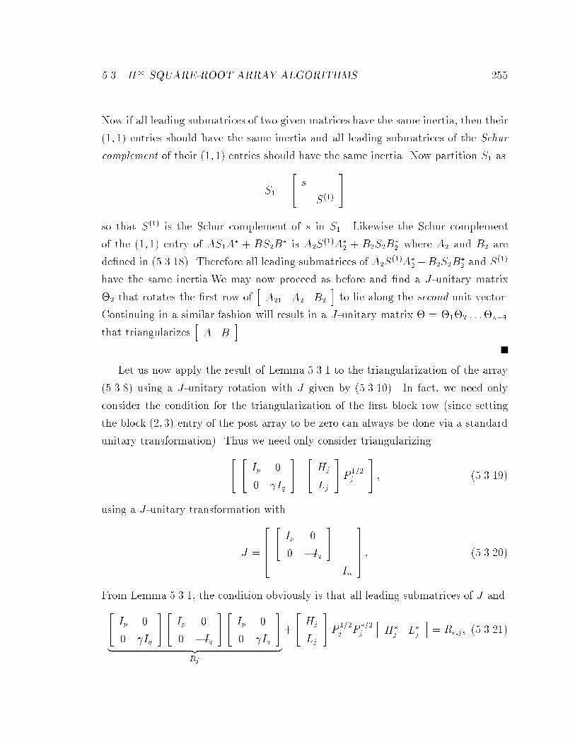
���� H� SQUARE�ROOT ARRAY ALGORITHMS ��
Now if all leading submatrices of two given matrices have the same inertia� then their
��� �� entries should have the same inertia and all leading submatrices of the Schur
complement of their ��� �� entries should have the same inertia� Now partition S� as
S� �
�� s
S���
�
so that S��� is the Schur complement of s in S�� Likewise the Schur complement
of the ��� �� entry of AS�A� � BS�B� is A�S
���A�� � B�S�B
�� where A� and B� are
de�ned in ��������� Therefore all leading submatrices of A�S���A�
��B�S�B�� and S���
have the same inertia�We may now proceed as before and �nd a J �unitary matrix
�� that rotates the �rst row ofhA�� A� B�
ito lie along the second unit vector�
Continuing in a similar fashion will result in a J �unitary matrix � � ���� � � ��n��
that triangularizeshA B
i�
Let us now apply the result of Lemma ����� to the triangularization of the array
������� using a J �unitary rotation with J given by ��������� In fact� we need only
consider the condition for the triangularization of the �rst block row �since setting
the block � � �� entry of the post array to be zero can always be done via a standard
unitary transformation�� Thus we need only consider triangularizing
���� Ip �
� �Iq
�
�� Hj
Lj
�P ���
j
� � �������
using a J �unitary transformation with
J �
�����
�� Ip �
� �Iq
�
In
���� � ����� ��
From Lemma ������ the condition obviously is that all leading submatrices of J and
�� Ip �
� �Iq
��� Ip �
� �Iq
��� Ip �
� �Iq
�
�z �Rj
�
�� Hj
Lj
�P ���
j P���j
hH�
j L�j
i� Re�j � ����� ��

��CHAPTER �� SQUARE�ROOTARRAYSANDCHANDRASEKHARRECURSIONS
have the same inertia� But this is precisely the condition required for the existence
of an H� a posteriori �lter" �See Lemma ����� and Corollary ������� This result is
quite amazing � it states that an H� �a posteriori� �lter exists if� and only if� the
prearray can be triangularized� i�e�� if� and only if� the square�root algorithm can be
performed and does not break down�
This observation should now reinforce our conviction that the most natural way
of studying H� problems is through the geometry of inde�nite metric spaces� As
just seen� this approach allowed us to immediately generalize the form of the con�
ventional square�root array algorithm to the H� setting �by introducing inde�nite
square�roots�� Most importantly� once this was done� the conditions for triangulariz�
ing arrays� as forced upon us by the geometry of Krein spaces� directly led us to the
conditions for the existence of H� �lters�� Thus in square�root implementations of
H� �lters the existence conditions are built into the algorithms themselves� so that
there is no need to check for them separately�
Now that we have settled the existence question� let us return to triangularizing
the prearray �������� so that we can write�
�����
�� Ip �
� �Iq
�
�� Hj
Lj
�P ���
j �
� FjP���j Gj
�����j �
�� A � �
B C �
� � ����� �
where A and C are lower triangular� and where �j is J �unitary with J as in ���������
The array on the left hand side of ����� � is referred to as the pre�array and the array
on the right hand side as the post�array� To identify the elements A� B and C in the
post array let us square both sides of ����� � and use the fact that �j is J �unitary�
Therefore
�����
�� Ip �
� �Iq
�
�� Hj
Lj
�P ���
j �
� FjP���j Gj
�����jJ�
�j �z �
J
��������
�� Ip �
� �Iq
� �
P���j
hH�
j L�j
iP���j F �
j
� G�j
�������
�This phenomenon will occur again and again in this thesis� We shall shortly encounter it oncemore when we study the fast Chandrasekhar recursions�

���� H� SQUARE�ROOT ARRAY ALGORITHMS ��
�
�� A � �
B C �
�J
�����A� B�
� C�
� �
���� � ����� ��
Equating the ��� �� blocks on the left hand and right hand sides of ����� �� yields
�� Ip �
� ���Iq
��
�� Hj
Lj
�Pj
hH�
j L�j
i� A
�� Ip �
� �Iq
�A��
The left hand side of the above relation is simply Re�j � Therefore A is an inde�nite
square�root of the Re�j � and we can write
A � R���e�j � R
���e�j
�� Ip �
� �Iq
�R���
e�j � Re�j� ����� ��
Equating the � � �� blocks on the left hand and right hand sides of ����� �� yields
FjPj
hH�
j L�j
i� B
�� Ip �
� �Iq
�A��
Therefore
B � FjPj
hH�
j L�j
iR����e�j
�� Ip �
� �Iq
� �
so that we can write
B � #Kp�j � Kp�jR���e�j � ����� ��
Equating the � � � blocks on the left hand and right hand sides of ����� �� yields
FjPjF�j �GjG
�j � B
�� Ip �
� �Iq
�B� � CC�
� Kp�jR���e�j
�� Ip �
� �Iq
�R���
e�j K�p�j � CC�
� Kp�jRe�jK�p�j � CC��
Therefore
CC� � FjPjF�j �GjG
�j �Kp�jRe�jK
�p�j � Pj���

��CHAPTER �� SQUARE�ROOTARRAYSANDCHANDRASEKHARRECURSIONS
so that we may write
C � P���j�� � P
���j��P
���j�� � Pj��� ����� ��
We can now summarize our results as follows�
Theorem ���� �H� A Posteriori Square�Root Algorithm� The H� a poste�
riori �ltering problem with level � has a solution if� and only if� for all j � �� � � � � i
there exist J�unitary matrices �with J given by �������� �j� such that�����
�� Ip �
� �Iq
�
�� Hj
Lj
�P ���
j �
� FjP���j Gj
�����j �
�� R
���e�j � �
Kp�jR���e�j P
���j�� �
� ����� ��
where the algorithm is initialized with� P� � ��� If this is the case� then all possible
H� a posteriori �lters� sjjj � Ff�j�y�� � � � yj�� are given by any choices that yield�
kXj�
�� yj �Hj �xj
sjjj � Lj �xj
��
R��e�j
�� yj �Hj�xj
sjjj � Lj�xj
� � �� � � k � i
where �xj satis�es the recursion�
�xj�� � Fj�xj �Kp�j
�� yj �Hj�xj
sjjj � Lj�xj
� � �x� � ��
In the H� a priori �ltering problem we need to begin with the pre�array�����
�� �Iq �
� Ip
�
�� Lj
Hj
�P ���
j �
� FjP���j Gj
���� � ����� ��
and with
J �
��������
�� �Iq �
� Ip
�
In
Im
�������� ����� �
Note the reversal of the order of the fHj � Ljg as compared to the a posteriori case��
Using similar arguments we may prove the following result�

���� H� SQUARE�ROOT ARRAY ALGORITHMS �
Theorem ���� �H� A Priori Square�Root Algorithm� The H� a priori �l�
tering problem with level � has a solution if� and only if� for all j � �� � � � � i there
exist J�unitary matrices �with J given by ����� ��� �j� such that
�����
�� �Iq �
� Ip
�
�� Lj
Hj
�P ���
j �
� FjP���j Gj
�����j �
�� R
���e�j � �
Kp�jR���e�j P
���j�� �
� ��������
where the algorithm is initialized with� P� � ��� If this is the case� then all possible
H� a priori �lters� sj � Ff�j�y�� � � � yj���� are given by any choices that yield�
kXj�
�� sj � Lj �xj
yj �Hj �xj
��
R��e�j
�� sj � Lj�xj
yj �Hj�xj
� � �� � � k � i
where �xj satis�es the recursion�
�xj�� � Fj�xj �Kp�j
�� sj � Lj�xj
yj �Hj�xj
� � �x� � ��
Note that� as in the H�case� the quantities necessary to update the square�root
array and to calculate the desired estimates may all be found from the triangularized
post�array�
In conventional Kalman �ltering� square�root arrays are preferred since the positive�
de�niteness of the matrices is guaranteed� and since the �j are unitary� which im�
proves the numerical stability of the algorithm� In the H� setting� the square�root
arrays guarantee that the various matrices have their appropriate inertia$ however�
the �j are no longer unitary but J �unitary� Therefore the numerical aspects need
further investigation�
An interesting aspect of Theorems ����� and ���� is that there is no need to
explicitly check for the existence conditions required ofH� �lters �see Theorems �� ��
and �� � �� These conditions are built into the square�root algorithms themselves� if
the algorithms can be performed an H� estimator of the desired level exists� and if
they cannot be performed such an estimator does not exist�

��CHAPTER �� SQUARE�ROOTARRAYSANDCHANDRASEKHARRECURSIONS
����� The Central Filters
In the previous section we obtained a square�root version of the parametrization of
all H� a posteriori and a priori �lters� Perhaps the most important �lters in these
classes are the so�called central �lters� which� as we have seen earlier� possess the
additional properties of being maximum�entropy and risk�sensitive�optimal �lters� as
well as being the solution to certain quadratic dynamic games �see Chapters �� � abd
��� In this section we shall develop square�root algorithms speci�cally for such central
�lters� As expected� the observer gains for the central �lters turn out to be readily
obtainable from the square�root algorithms of Theorems ����� and ���� �
Let us begin by recalling �from Theorem �� ��� the central H� a posteriori �lter
recursions�
�xj��jj�� � Fj�xjjj �Ks�j���yj�� �Hj��Fj�xjjj�� ��������
where the desired estimate is given by �sjjj � Lj �xjjj� and where the gain vector is
given by
Ks�j � PjH�j �Ip �HjPjH
�j ���� ������ �
We will now show how to obtain the above gain vector from the a posteriori square�
root recursions�
To this end� let us �rst note that we can rewrite the a posteriori square�root
algorithm of Theorem ����� via the following two�step procedure�
�����
�� Ip �
� �Iq
�
�� Hj
Lj
�P ���
j
� P���j
�����
���j �
�� R
���e�j �
Kf�jR���e�j P
���jjj
� � ��������
hFjP
���jjj Gj
i����j �
hP���j�� �
i��������
where ����j is J �unitary� with J � Ip � ��Iq� � In� and �
���j is unitary� Note that
the above two�step procedure is the H� analog of Algorithm �� � �� In the above
recursions� we of course have
Kf�j � Pj
hH�
j L�j
iR��e�j � ��������

���� H� SQUARE�ROOT ARRAY ALGORITHMS ��
with
Re�j �
�� Ip �
� ���Iq
��
�� Hj
Lj
�Pj
hH�
j L�j
i� ��������
Now in ��������� R���e�j can be any square�root of Re�j� Let us study the consequences
of choosing a lower triangular square�root� To do so� consider the following triangular
factorization of Re�j�
�� Ip �
LjPjH�j �Ip �HjPjH
�j ��� Iq
��� Ip �HjPjH
�j �
� �%j
��� Ip �Ip �HjPjH
�j ���HjPjL
�j
� Iq
� �
��������
where we have de�ned the Schur complement�
�%j�� ���Iq � LjPjL
�j � LjPjH
�j �Ip �HjPjH
�j ���HjPjL
�j �
Note that the inertia condition on Re�j implies that %j � �� so that we may write
Re�j � R���e�j SR
���e�j � ��������
with
R���e�j �
�� Ip �
LjPjH�j �Ip �HjPjH
�j ��� Iq
��� �Ip �HjPjH
�j �
��� �
� %���j
�
�
�� �Ip �HjPjH
�j �
��� �
LjPjH�j �Ip �HjPjH
�j ����� %���
j
� � �������
and S �
�� Ip
�Iq
�� Now the � � �� block entry in the postarray of �������� is given
by
Kf�jR���e�j � Pj
hH�
j L�j
iR����e�j
� Pj
hH�
j L�j
i �� �Ip �HjPjH�j ����� �Ip �HjPjH
�j ���HjPjL
�j%
����j
� %����j
�
� Pj
hH�
j �Ip �HjPjH�j ����� �
i� ��������
where � denotes irrelevant entries�
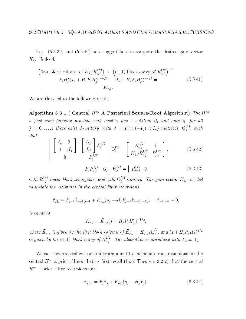
� CHAPTER �� SQUARE�ROOTARRAYSANDCHANDRASEKHARRECURSIONS
Eqs� ������� and �������� now suggest how to compute the desired gain vector
Ks�i� Indeed�
�rst block column of Kf�jR
���e�j
�� ��� �� block entry of R���
e�j
����
PjH�j �Ip �HjPjH
�j ����� � �Ip �HjPjH
�j ����� �
Ks�j �
��������
We are thus led to the following result�
Algorithm ���� � Central H� A Posteriori Square�Root Algorithm� The H�
a posteriori �ltering problem with level � has a solution if� and only if� for all
j � �� � � � � i there exist J�unitary �with J � Ip � ��Iq� � In� matrices� ����j � such
that �����
�� Ip �
� �Iq
�
�� Hj
Lj
�P ���
j
� P���j
�����
���j �
�� R
���e�j �
Kf�jR���e�j P
���jjj
� � ������ �
hFjP
���jjj Gj
i����j �
hP���j�� �
i��������
with R���e�j lower block triangular� and with ����
j unitary� The gain vector Ks�j needed
to update the estimates in the central �lter recursions
�xjjj � Fj���xj��jj�� �Ks�j�yj �HjFj���xj��jj���� �x��j�� � ��
is equal to
Ks�j � #Ks�j�I �HjPjH�j ������
where #Ks�j is given by the �rst block column of #Kf�j � Kf�jR���e�j � and �I�HjPjH
�j �
���
is given by the ��� �� block entry of R���e�j � The algorithm is initialized with P� � ���
We can now proceed with a similar argument to �nd square�root recursions for the
central H� a priori �lters� Let us �rst recall �from Theorem �� � � that the central
H� a priori �lter recursions are
�xj�� � Fj�xj �Ka�j�yj �Hj�xj�� ��������

���� H� SQUARE�ROOT ARRAY ALGORITHMS ��
where the desired estimate is given by �sj � Lj �xj� and where the gain vector is given
by
Ka�j � Fj�PjH
�j �Ip �Hj
�PjH�j ���� ��������
with
�Pj � Pj � PjL�j ���
�Iq � LjPjL�j ���LjPj � ��������
We will now show how to obtain the above gain vector from the a priori square�root
recursions�
�����
�� �Iq �
� Ip
�
�� Lj
Hj
�P ���
j �
� FjP���j Gj
�����j �
�� R
���e�j � �
Kp�jR���e�j P
���j�� �
� ��������
Note now that�
Kp�j � FjPj
hL�j H�
j
iR��e�j � ��������
with
Re�j �
�� ���Iq �
� Ip
��
�� Lj
Hj
�Pj
hL�j H�
j
i� �������
As mentioned earlier� R���e�j in �������� can be any inde�nite square�root of Re� Let us�
once more� study the consequences of choosing a lower triangular square�root� To do
so� consider the following block lower�diagonal�upper triangular factorization of the
matrix� Re�j �
�� Iq �
����Hj�PjL
�j Ip
��� ���Iq � LjPjL
�j �
� Ip �Hj�PjH
�j
��� Iq ����Lj
�PjH�j
� Ip
� �
��������
where we have used the facts that�
HjPjL�j ���
�Iq � LjPjL�j��� � ����Hj
�PjL�j �
and� for the Schur complement�
Ip �HjPjH�j �HjPjL
�j ���
�Iq � LjPjL�j ���LjPjH
�j � Ip �Hj
�PjH�j �

��CHAPTER �� SQUARE�ROOTARRAYSANDCHANDRASEKHARRECURSIONS
Now the inertia conditions on Re�j require that� ����Hj�PjL
�j � � and Ip�Hj
�PjH�j �
�� so that we may write�
Re�j � R���e�j SR
���e�j � ��������
with
R���e�j �
�� ���Iq � LjPjL
�j ���� �
����Hj�PjL
�j ��
�Iq � LjPjL�j���� �Ip �Hj
�PjH�j �
���
� � ������ �
and S �
�� �Iq
Ip
�� Now the � � �� block entry in the postarray of �������� is given
by
Kp�jR���e�j � FjPj
hL�j H�
j
iR����e�j
� FjPj
hL�j H�
j
i �� ���Iq � LjPjL�j ����� ���Lj
�PjH�j �Ip �Hj
�PjH�j �����
� �Ip �Hj�PjH
�j �����
�
� FjPj
h� ����L�jLj
�Pj � In�H�j �Ip �Hj
�PjH�j �����
i
� Fj
h� �PjH
�j �Ip �Hj
�PjH�j �����
i� ��������
where in the last step we have used the �readily veri�ed� identity�
Pj����L�jLj
�Pj � In� � �Pj �
and where � denotes irrelevant entries�
Eqs� ������ � and �������� now suggest how to compute the desired gain vector
Ka�i� Indeed�
second block column of Kp�jR
���e�j
�� � � � block entry of R
���e�j
����
Fj�PjH
�j �Ip �Hj
�PjH�j ����� � �Ip �Hj
�PjH�j ����� �
Ka�j�
��������
We are thus led to the following result�
Algorithm ���� �Central H� A Priori Square�Root Algorithm� The H� a
priori �ltering problem with level � has a solution if� and only if� for all j � �� � � � � i

���� H� CHANDRASEKHAR RECURSIONS ��
there exist J�unitary matrices �with J � ��Iq�� Ip � In � Im�� �j � such that
�����
�� �Iq �
� Ip
�
�� Lj
Hj
�P ���
j �
� FjP���j Gj
�����j �
�� R
���e�j � �
Kp�jR���e�j P
���j�� �
� ��������
with R���e�j lower block triangular� The gain vector Ka�i needed to update the estimates
in
�xj�� � Fj�xj �Ka�j�yj � Fj�xj�� �x� � ��
is equal to
Ka�j � #Ka�j�I �Hj�PjH
�j ������
where #Ka�j is given by the second block column of #Kp�j � Kp�jR���e�j � and �I�Hj
�PjH�j �
���
is given by the � � � block entry of R���e�j � The algorithm is initialized with P� � ���
��� H Chandrasekhar Recursions
The conventional Kalman �lter and square�root array recursions of Sec� �� both
require O�n�� operations per iteration �where n is the number of states in the state�
space model�� However� when the state�space model is time�invariant �or if the time�
variation is structured in a certain way� the Chandrasekhar recursions o�er an algo�
rithm that requires O�n�� operations per iteration Kai� � MSK��� SK�a��
In what follows we shall assume a time�invariant state�space model of the form���xj�� � Fxj �Guj � x�
yj � Hxj � vj�������
where the fuj� vjg are disturbances whose nature depends on the criterion being used�
and where the fyjg are the observed outputs� In the H� case� where the fuj� vjg are
zero mean independent random variables� we shall also assume that the covariances
of the fuj� vjg are constant� i�e� Qj � Q � � and Rj � R � �� for all j� As before�
we are interested in obtaining estimates of some linear combinations of the states�
sj � Ljxj� and� in particular� the �ltered estimates� �sjjj � Lj �xjjj� and predicted
estimates� �sj � Lj�xj� that use the observations fykgjk� and fykg
j��k�� respectively�

��CHAPTER �� SQUARE�ROOTARRAYSANDCHANDRASEKHARRECURSIONS
Under the aforementioned assumptions� it turns out that we can write
Pj�� � Pj � MjSMj � j� ����� �
whereMj is a n�dmatrix and S is a d�d signature matrix �i�e� a diagonal matrix with
�� and �� on the diagonal�� Thus� for time�invariant state�space models� Pj�� � Pj
has rank d for all j and in addition has constant inertia� In several important cases�
d can be much less than n� When this is true� propagating the smaller matrices Mj�
which is equivalent to propagating the Pj � can o�er computational reductions� This
what is done by the Chandrasekhar recursions �see Kai���� App� II��
In the conventional Chandrasekhar recursions� one begins with the pre�array
�� R
���e�j HMj
#Kp�j FMj
� � �������
where R���e�j R
���e�j � Re�j � R �HPjH
� and #Kp�j � Kp�jR����e�j � and triangularizes the
array using a J �unitary matrix �j where J is given by
�� Ip
S
�� The result of
this triangularization gives us the various quantities of interest for propagating the
Kalman �lter recursions�
Algorithm ����� �Conventional Chandrasekhar Recursions� The gain vector
Kp�j � #Kp�jR����e�j necessary to obtain the state estimates in the conventional Kalman
�lter
�xj�� � F �xj �Kp�j�yj �H�xj�� �x� � ��
can be computed using
�� R
���e�j HMj
#Kp�j FMj
��j �
�� R
���e�j�� �
#Kp�j�� Mj��
� � �������
where �j is any J�unitary matrix �with J � Ip � S� that triangularizes the above
pre�array� The algorithm is initialized with
Re�� � R�H��H�� #Kp�� � F��H
�R���e�� �
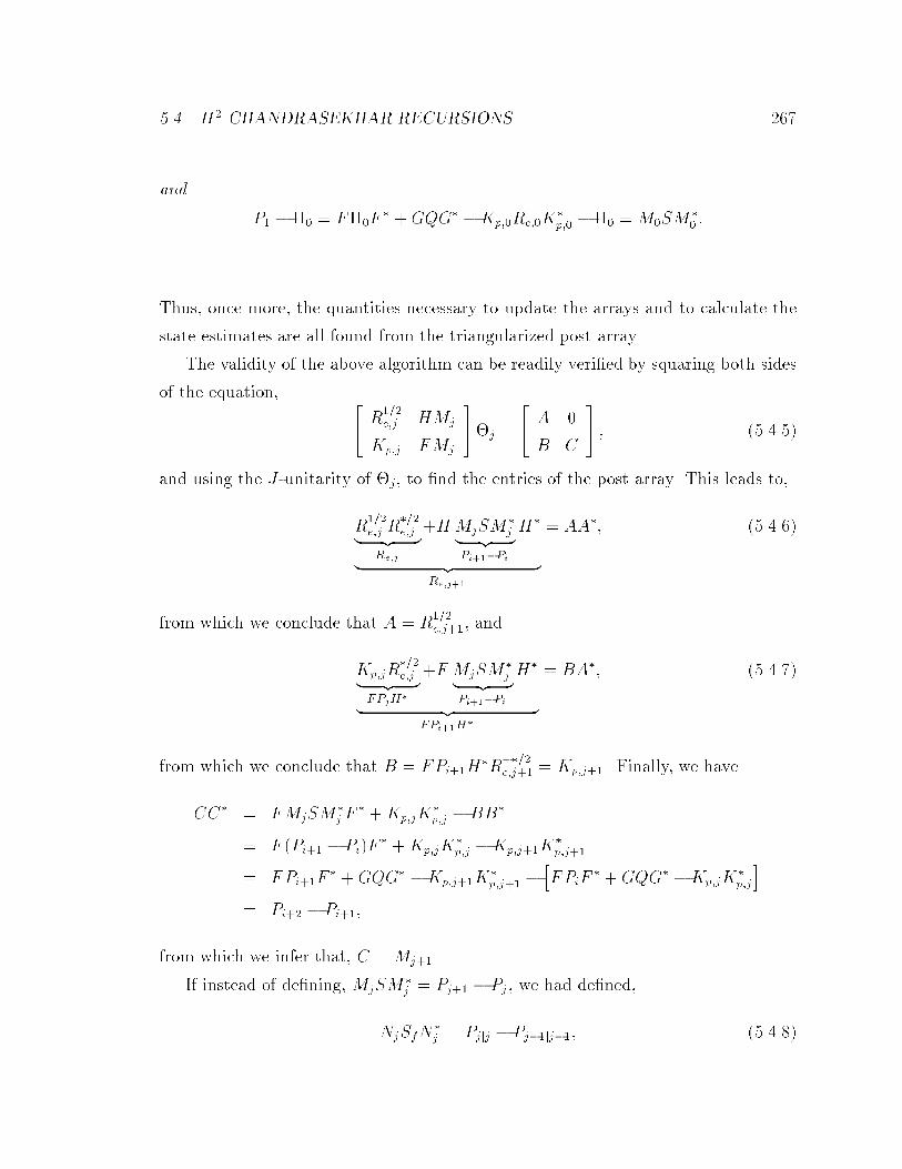
���� H� CHANDRASEKHAR RECURSIONS ��
and
P� ��� � F��F� �GQG� �Kp��Re��K
�p�� ��� �M�SM
�� �
Thus� once more� the quantities necessary to update the arrays and to calculate the
state estimates are all found from the triangularized post array�
The validity of the above algorithm can be readily veri�ed by squaring both sides
of the equation� �� R
���e�j HMj
#Kp�j FMj
��j �
�� A �
B C
� � �������
and using the J �unitarity of �j� to �nd the entries of the post array� This leads to�
R���e�j R
���e�j �z �
Re�j
�HMjSM�j �z �
Pi���Pi
H�
�z �Re�j��
� AA�� �������
from which we conclude that A � R���e�j��� and
#Kp�jR���e�j �z �
FPjH�
�F MjSM�j �z �
Pi���Pi
H�
�z �FPi��H�
� BA�� �������
from which we conclude that B � FPi��H�R
����e�j�� � #Kp�j��� Finally� we have
CC� � FMjSM�j F
� � #Kp�j#K�p�j �BB�
� F �Pi�� � Pi�F� � #Kp�j
#K�p�j � #Kp�j��
#K�p�j��
� FPi��F� �GQG� � #Kp�j��
#K�p�j�� �
hFPiF
� �GQG� � #Kp�j#K�p�j
i
� Pi�� � Pi���
from which we infer that� C �Mj���
If instead of de�ning� MjSM�j � Pj�� � Pj � we had de�ned�
NjSfN�j � Pjjj � Pj��jj��� �������

��CHAPTER �� SQUARE�ROOTARRAYSANDCHANDRASEKHARRECURSIONS
where Pjjj � E�xjjj�x�jjj is the �ltered state error variance� which satis�es the recursion�
Pjjj � FPj��jj��F� �GQG� �Kf�jRe�jK
�f�j� ������
withKf�j � PjHR��e�j � then it is also possible to obtain the following �so�called� �ltered
form of the Chandrasekhar recursions��
Algorithm ����� �Conventional Chandrasekhar Recursions� Filtered Form�
The gain vector Kf�j � #Kf�jR����e�j necessary to obtain the state estimates in the �ltered
form of the conventional Kalman �lter
�xjjj � F �xj��jj�� �Kf�j�yj �HF �xj��jj���� �x��j�� � ��
can be computed using
�� R
���e�j HFNj
#Kf�j FNj
��j �
�� R
���e�j�� �
#Kf�j�� Nj��
� � ��������
where �j is any J�unitary matrix �with J � Ip � Sf� that triangularizes the above
pre�array� The algorithm is initialized with
Re�� � R�H��H�� #Kf�� � ��H
�R���e�� �
and
F���P� ����F�� � �� � F��GQG�F�� �Kf��Re��K
�f�� � F����F
�� � N�SfN�� �
Note that compared to the square�root formulas� the size of the pre�array in the
Chandrasekhar recursions has been reduced from �p�n���p�n�m� to �p�n���p�d�
wherem and p are the dimensions of the driving disturbance and output� respectively�
and where n is the number of the states� Thus the number of operations for each
iteration has been reduced from O�n�� to O�n�d�� with d typically much less than n�
�Note that in this case it can also be shown that Pj��jj���Pjjj has constant inertia� given by theinertia of the signature matrix� Sf � for all j� This follows from the fact that Pj�� � FPjjjF
��GQG��so that Pj�� � Pj � F Pjjj � Pj��jj��F
��
���� H� CHANDRASEKHAR RECURSIONS �
��� H� Chandrasekhar Recursions
In this section we shall derive the H� counterparts of the �fast� H� Chandrasekhar
recursions of the previous section� We shall essentially see that� when the underlying
state�space model is time�invariant� all the arguments necessary for the development
of these algorithms go through� provided that we consider the geometry of inde�nite
spaces� We �rst give the general recursions� and then specialize them to obtain the
central �lters�
����� The General Case
Recall from Sec� ��� that the Chandrasekhar recursions apply to time�invariant state�
space models� Therefore the Krein state�space models whose Kalman �lters yield the
H� estimators must be time�invariant as well� Indeed for theH� a posteriori �ltering
problem� we need to assume the following Krein state�space model
���������
xi�� � Fxi �Gui�� yi
siji
� �
�� H
L
�xi � vi
i � � �������
with
h
�����ui
vi
x�
���� �
�����uj
vj
x�
����i �
��������
Im�ij
�� Ip �
� ���Iq
� �ij
��
�������� ����� �
Suppose that the matrix �� can be chosen such that P� ��� has low rank� In other
words�
P� ��� � F��F� �GG� �Kp��Re��K
�p�� ��� � M�SM
�� � �������
where M� is a n� d matrix �typically d n� and S is a d� d signature matrix� and�
of course�
Kp�j � FPj
hH� L�
iR��e�j and Re�j �
�� Ip �
� ���Iq
��
�� H
L
�Pj
hH� L�
i�
�������

��CHAPTER �� SQUARE�ROOTARRAYSANDCHANDRASEKHARRECURSIONS
We shall presently show by induction that under the assumptions of a time�invariant
state�space model� if the a posteriori H� �ltering problem has a solution for all j�
then Pj���Pj has rank d for all j and that we may actually write Pj���Pj � MjSM�j �
Consider the following pre�array�����R���e�j
�� H
L
�Mj
#Kp�j FMj
���� � �������
which is the extension of the pre�array in ������� to the Krein state�space model �������
of the H� a posteriori �ltering problem� Now the H� a posteriori �ltering problem
will have a solution if� and only if� all leading submatrices of R and Re�j �or Re�j��� for
that matter� have the same inertia� In view of Lemma ����� this implies that the H�
a posteriori �ltering problem with level � will have a solution if� and only if� there
exists a J �unitary matrix �j that triangularizes ������� where
J �
�����
�� Ip �
� �Iq
�
S
���� � �������
Therefore we can write�����R���e�j
�� H
L
�Mj
#Kp�j FMj
�����j �
�� A �
B C
� � �������
To identify the elements A� B and C in the post�array we square both sides of �������
and use the fact that �j is J �unitary� Therefore�����R���e�j
�� H
L
�Mj
#Kp�j FMj
�����jJ�
�j �z �
J
�� R
���e�j
#K�p�j
M�j
hH� L�
iMjF
�
� �
�� A �
B C
�J
�� A� B�
� C�
� �
�������
Equating the ��� �� blocks in ������� yields�
A
�� Ip �
� �Iq
�A� � R
���e�j
�� Ip �
� �Iq
�R���
e�j �
�� H
L
�MjSM
�j
hH� L�
i
���� H� CHANDRASEKHAR RECURSIONS ��
� Re�j �
�� H
L
� �Pj�� � Pj�
hH� L�
i
� Rj �
�� H
L
�Pj��
hH� L�
i
� Re�j���
Therefore A is the inde�nite square�root of Re�j���
A � R���e�j��� ������
Equating the � � �� blocks in ������� yields�
B
�� Ip �
� �Iq
�A� � #Kp�j
�� Ip �
� �Iq
�R���
e�j � FMjSM�j
hH� L�
i
� Kp�jRe�j � F �Pj�� � Pj�hH� L�
i
� FPj
hH� L�
i� F �Pj�� � Pj�
hH� L�
i
� FPj��
hH� L�
i�
Therefore
B � FPj��
hH� L�
iA��
�� Ip �
� �Iq
�
� FPj��
hH� L�
iR����e�j��
�� Ip �
� �Iq
� � #Kp�j��� ��������
Equating the � � � blocks in ������� yields
CSC��B
�� Ip �
� �Iq
�B� � #Kp�j
�� Ip �
� �Iq
� #K�
p�j � FMjSM�j F
��
Therefore
CSC� �Kp�j��Re�j��K�p�j�� � Kp�jRe�jK
�p�j � F �Pj�� � Pj�F
��
We can now write
CSC� � FPj��F� �Kp�j��Re�j��K
�p�j�� �GG� � �FPjF
� �Kp�jRe�jK�p�j �GG��
� Pj�� � Pj���

� CHAPTER �� SQUARE�ROOTARRAYSANDCHANDRASEKHARRECURSIONS
and �nally
C � Mj��� ��������
Note that our derivation of C also shows that if P�� P� �M�SM�� then Pi�� � Pi �
MiSM�i for all i�
We have thus established�����R���e�j
�� H
L
�Mj
#Kp�j FMj
�����j �
�� R
���e�j�� �
#Kp�j�� Mj��
� �
from which we can now give the following �fast� Chandrasekhar version of the para�
metrization of all H� a posteriori �lters�
Theorem ����� �H� A Posteriori Chandrasekhar Recursions� The H� a pos�
teriori �ltering problem with level � has a solution if� and only if� all leading subma�
trices of
R �
�� Ip �
� ���Iq
� and Re�� �
�� Ip �
� ���Iq
��
�� H
L
���
hH� L�
i
have the same inertia� and if for all j � �� � � � � i there exist J�unitary matrices �with
J � Ip � ��Iq�� S�� �j� such that
�����
R���e�j
�� H
L
�Mj
Kp�jR���e�j FMj
�����j �
�� R
���e�j�� �
Kp�j��R���e�j�� Mj��
� ������ �
where the algorithm is initialized with� Re��� Kp�� � F��
hH� L�
iR��e��� and
P� ��� � F��F� �GQG� �Kp��Re��K
�p�� ��� � M�SM
�� � ��������
If this is the case� then all possible H� a posteriori �lters� sjjj � Ff�j�y�� � � � yj�� are
given by any choices that yield�
kXj�
�� yj �Hj �xj
sjjj � Lj �xj
��
R��e�j
�� yj �Hj�xj
sjjj � Lj�xj
� � �� � � k � i

���� H� CHANDRASEKHAR RECURSIONS ��
where �xj satis�es the recursion�
�xj�� � Fj�xj �Kp�j
�� yj �Hj�xj
sjjj � Lj�xj
� � �x� � ��
In the H� a priori �ltering problem� we need� instead� to start with the Krein
state�space model����������
xi�� � Fxi � Gui�� si
yi
� �
�� L
H
�xi � vi
i � � ��������
with
h
�����ui
vi
x�
���� �
�����uj
vj
x�
����i �
��������
Im�ij
�� ���Iq �
� Ip
� �ij
��
�������� ��������
and with the prearray� �����
R���e�j
�� L
H
�Mj
Kp�jR���e�j FMj
���� � ��������
where now
Kp�j � FPj
hL� H�
iR��e�j and Re�j �
�� ���Iq �
� Ip
��
�� L
H
�Pj
hL� H�
i�
��������
Note that the only di�erence with the a posteriori case is in the order of the matrices
fH�Lg��
Proceeding with an argument similar to what was done in the a posteriori case�
we can show the following result�
Theorem ����� �H� A Priori Chandrasekhar Recursions� The H� a priori
�ltering problem with level � has a solution if� and only if� all leading submatrices of
R �
�� ���Iq �
� Ip
� and Re�� �
�� ���Iq �
� Ip
��
�� L
H
���
hL� H�
i

��CHAPTER �� SQUARE�ROOTARRAYSANDCHANDRASEKHARRECURSIONS
have the same inertia� and if for all j � �� � � � � i there exist J�unitary matrices �with
J � ��Iq�� Ip � S�� �j� such that
�����
R���e�j
�� L
H
�Mj
Kp�jR���e�j FMj
�����j �
�� R
���e�j�� �
Kp�j��R���e�j�� Mj��
� ��������
where the algorithm is initialized with� Re��� Kp�� � F��
hL� H�
iR��e��� and
P� ��� � F��F� �GQG� �Kp��Re��K
�p�� ��� � M�SM
�� � �������
If this is the case� then all possible H� a priori �lters� sj � Ff�j�y�� � � � yj���� are
given by any choices that yield�
kXj�
�� sj � Lj �xj
yj �Hj �xj
��
R��e�j
�� sj � Lj�xj
yj �Hj�xj
� � �� � � k � i
where �xj satis�es the recursion�
�xj�� � Fj�xj �Kp�j
�� sj � Lj�xj
yj �Hj�xj
� � �x� � ��
Note that compared to the H� square�root formulas� the size of the pre�array in
theH� Chandrasekhar recursions has been reduced from �p�q�n���p�q�n�m� to
�p�q�n���p�q�d� wherem� p and q are the dimensions of the driving disturbance�
output and states to be estimated� respectively� and where n is the number of the
states� Thus the number of operations for each iteration has been reduced from O�n��
to O�n�d� with d typically much less than n�
As in the square�root case� the Chandrasekhar recursions do not require explicitly
checking the positivity conditions of Theorems �� �� and �� � � if the recursions
can be carried out an H� estimator of the desired level exists� and if not� such an
estimator does not exist�

���� H� CHANDRASEKHAR RECURSIONS ��
����� The Central Filters
The preceding section gave �fast� Chandrasekhar versions of all possible H� a pos�
teriori and a priori �lters� Here we shall specialize these recursions to the central a
posteriori and a priori �lters� We shall show that the observer gains for these �lters
can be readily obtained from the post�arrays of Theorems ����� and ���� � provided
we insist on �block� lower triangular square�roots for R���e�j � The development closely
follows that of Sec� ���� and uses the important facts �established in Sec� ���� � that
if R���e�j is lower triangular� then Ks�j � the gain vector for the central a posteriori �lter�
is given by�
Ks�j � �rst block column of Kf�jR
���e�j
�� ��� �� block entry of R���
e�j
���� ����� ��
and Ka�j� the gain vector for the central a priori �lter� is given by�
Ka�j � second block column of Kp�jR
���e�j
�� � � � block entry of R���
e�j
����
����� ��
The following result are now readily establishable� �The proofs are straightforward
and will be omitted for brevity��
Algorithm ����� �Central H� A Posteriori Chandrasekhar Recursions� The
H� a posteriori �ltering problem with level � has a solution if� and only if� all leading
submatrices of
R �
�� Ip �
� ���Iq
� and Re�� �
�� Ip �
� ���Iq
��
�� H
L
���
hH� L�
i
have the same inertia� and if for all j � �� � � � � i there exist J�unitary matrices� �j�
�where J � Ip � ��Iq�� Sf� such that�����
R���e�j
�� H
L
�FNj
Kf�jR���e�j FNj
�����j �
�� R
���e�j�� �
Kf�jR���e�j�� Nj��
� ����� �
with R���e�j and R
���e�j�� block lower triangular� The algorithm is initialized with� Re���
Kf�� � ��
hH� L�
iR��e��� and
F���P� ����F�� � �� � F��GQG�F�� �Kf��Re��K
�f�� � F����F
�� � N�SfN�� �

��CHAPTER �� SQUARE�ROOTARRAYSANDCHANDRASEKHARRECURSIONS
The gain vector Ks�j needed to update the estimates in the central �lter recursions
�xjjj � Fj���xj��jj�� �Ks�j�yj �HjFj���xj��jj���� �x��j�� � ��
is equal to
Ks�j � #Ks�j�I �HjPjH�j ������
where #Ks�j is given by the �rst block column of #Kf�j � Kf�jR���e�j � and �I�HjPjH
�j �
���
is given by the ��� �� block entry of R���e�j �
Algorithm ����� �Central H� A Priori Chandrasekhar Recursions� The H�
a priori �ltering problem with level � has a solution if� and only if� all leading sub�
matrices of
R �
�� ���Iq �
� Ip
� and Re�� �
�� ���Iq �
� Ip
��
�� L
H
���
hL� H�
i
have the same inertia� and if for all j � �� � � � � i there exist J�unitary matrices� �j�
�where J � ��Iq�� Ip � S� such that
�����
R���e�j
�� L
H
�Mj
Kp�jR���e�j FMj
�����j �
�� R
���e�j�� �
Kp�j��R���e�j�� Mj��
� ����� ��
with R���e�j and R
���e�j�� block lower triangular� The algorithm is initialized with� Re���
Kp�� � F��
hL� H�
iR��e�� and
P� ��� � F��F� �GQG� �Kp��Re��K
�p�� ��� �M�SM
�� �
The gain vector Ka�i needed to update the estimates in
�xj�� � Fj�xj �Ka�j�yj � Fj�xj�� �x� � ��
is equal to
Ka�j � #Ka�j�I �Hj�PjH
�j ������
where #Ka�j is given by the second block column of #Kp�j � Kp�jR���e�j � and �I�Hj
�PjH�j �
���
is given by the � � � block entry of R���e�j �
���� CONCLUSION ��
��� Conclusion
In this chapter� we obtained square�root array algorithms and Chandrasekhar re�
cursions for the H� a posteriori and a priori �ltering problems� These algorithms
involve propagating the inde�nite square�roots of the quantities of interest� and have
the interesting property that the appropriate inertia of these quantities is preserved�
Moreover� the conditions for the existence of the H� �lters are built into the algo�
rithms� so that �lter solutions will exist if�and only if� the algorithms can be executed�
The conventional square�root arrays and Chandrasekhar recursions are preferred
because of their numerical stability �in the case of square�root arrays� and their re�
duced computational complexity �in the case of the Chandrasekhar recursions�� Since
the H� square�root arrays and Chandrasekhar recursions are the direct analogs of
their conventional counterparts� they may be more attractive for numerical imple�
mentation of H� �lters� However� since J �unitary rather than unitary operations are
involved� further numerical investigation is needed�
Our derivation of theH� square�root arrays and Chandrasekhar recursions demon�
strates a virtue of the Krein space approach to H� estimation and control$ the results
appear to be more di�cult to conceive and prove in the traditional H� approaches�
We should also mention that there are many variations of the conventional square�
root array and Chandrasekhar recursions� e�g� for control problems� and the methods
given here are directly applicable to extending these variations to the H� setting as
well� Finally� the algorithms presented here are equally applicable to risk�sensitive
estimation and control problems� and to quadratic dynamic games�
Chapter �
Duality and Control
This chapter deals with duality in �de�nite and inde�nite metric� linear spaces� Du�
ality here is introduced through the geometrical notion of dual bases for linear spaces
spanned by a set of nonorthogonal basis vectors� We shall see that� apart from having
conceptual value� duality is a useful tool in the study of various problems of inter�
est� In particular� it allows for a dual approach to �de�nite and inde�nite� quadratic
problems� A large part of this chapter is therefore devoted to the use of duality in
�H�� H�� game�theoretic and risk�sensitive� control� where �within the framework
presented here� the notion of duality is indispensable for obtaining the solution�
��� Introduction
In this chapter we return to the geometric viewpoint of Chapter �� We have already
seen the power of such a geometrical approach in unifying the treatment of �stochastic�
H� estimation and �deterministic� H� estimation problems� �where the solutions are
obtained by projecting� respectively in a Hilbert and Krein space� one vector onto the
linear span of another set of vectors�� in the introduction of the innovations process
�via Gram�Schmidt orthogonalization� for performing the canonical factorization of
�possibly inde�nite� Gramian matrices� and in the extension of conventional square�
root arrays and Chandrasekhar recursions to the H� setting� Here we shall introduce
a further natural consequence of adopting a geometric point of view more speci�cally�
��

���� INTRODUCTION ��
the study of dual bases and dual linear models� The concept of a dual basis is
one that has considerable �albeit� often conceptual� value in studying linear spaces
spanned by a set of nonorthogonal basis vectors� It also has several rami�cations
in particular� it shows how deterministic and stochastic least�squares problems can
be solved using a dual approach� it has certain implications to smoothing problems�
and� most importantly� it is very useful in the study of control problems �where the
duality between estimation and control has long been recognized��� We shall� in
fact� spend considerable time on a general linear�quadratic�regulator �LQR� control
problem with inde�nite weighting matrices� and its special cases in full information
and measurement feedback H� control�
The remainder of this chapter is organized as follows� In Sec� �� we begin by
considering a di�erent deterministic quadratic form to the one that had been studied
in Sec� ������ and whose stationary point was given by a Krein space projection�
These two deterministic quadratic forms are related by the fact that their coe�cient
matrices are inverses of one another� In Sec� ��� by considering the concept of a dual
basis� we obtain a geometric interpretation for the stationary point of the quadratic
form of Sec� ��� and in particular� show that it is given by a dual Krein space
projection� Moreover� we obtain various useful relationships �via certain dualities
and equivalences� that shed further light on the interplay between deterministic and
stochastic least�squares problems �see Table ������� In particular� in Sec� ��� we
show that� given any quadratic optimization problem� it can be solved in either one
of two ways by constructing an equivalent Krein space model� for which the solution
is given by a Krein space projection� or� by constructing a dual Krein space model�
for which the solution is given by the negative conjugate transpose of the operator
that yields the dual Krein space projection� Which one of these approaches to use
depends upon the application for estimation and adaptive �ltering problems it is
more natural to use the equivalent Krein space model� whereas for control problems
it more natural to use the dual Krein space model�
Now the dual bases span the orthogonal complement space� or the space of the
�See also the comments at the end of Sec� �������For di�erent approaches to duality consult �Wal�� and �Lue��

��� CHAPTER �� DUALITY AND CONTROL
smoothing errors� of the original bases� In Sec� ��� we show that when the original
basis has state�space structure� then the dual basis also has state�space structure�
�The dual state�space model is often referred to as the adjoint or complementary
state�space model�� In particular� we develop backwards�time� forwards�time and
mixed dual state�space models� and in Sec� � use the mixed dual state�space model
to obtain the so�called two �lter formulae for smoothing�
Sec� � considers the LQR �linear�quadratic�regulator� control problem with
�possibly� inde�nite weighting matrices� This problem is of interest since it subsumes�
as special cases� the problems of H�� H�� game�theoretic and risk�sensitive control�
We solve the LQR problem using duality� i�e�� we �rst construct the dual Krein
space model associated with the inde�nite LQR quadratic form �which is a Krein
space backwards�time dual state�space model� and then use the �negative conjugate
transpose of the operator that performs the� dual Krein space projection to �nd its
stationary point �and hence its solution�� The dual projection is performed by the
Krein space Kalman �lter associated with the backwards�time dual state�space model�
and the condition for the stationary point to be a minimum is given by certain inertia
requirements on Gramians readily available from the Krein space Kalman �lter� The
results of Sec� � are then used in Secs� �� and �� to solve the full information
and measurement feedback H� control problems� The solutions for both causal and
strictly causal controllers are given� and the measurement feedback problem�s solution
requires a separation principle that was earlier introduced in Sec� �����
��� An Alternative Scalar Quadratic Form
In Sec� ����� we saw that if we form a scalar quadratic form
J�z� y� �hz� y�
i �� Rz Rzy
Ryz Ry
����
�� z
y
��
where
�� Rz Rzy
Ryz Ry
��may be identi�ed as the Gramian of the the Krein space variables
fz�yg� then the stationary point of J�z� y� over z can be obtained via computing the

���� AN ALTERNATIVE SCALAR QUADRATIC FORM ���
projection of z onto L�y�� However� there is another scalar quadratic form that can
be constructed from the Gramian of fz�yg and that we have not yet considered� This
is what is done in the following Lemma�
Lemma ����� �Matrix to Scalar Second Order Form� The stationary point ydo
�over zd� of
I�zd� yd� �hzd� yd�
i �� Rz Rzy
Ryz Ry
���� zd
yd
��
is given by
ydo � �R��y Ryzz
d�
and
I�zd� ydo� � zd��Rz �RzyR��y Ryz�z
d�
Moreover� this stationary point is a minimum if� and only if�
Ry � ��
Proof� The proof involves the �lower�upper� triangular factorization of
�� Rz Rzy
Ryz Ry
��
and is straightforward�
Remark� Note that the coe�cient matrix appearing in the solution to the deter�
ministic problem of Lemma ���� is given by the negative conjugate transpose of the
coe�cient matrix appearing in the projection of z onto y� However� the condition for
a minimum� Ry � �� is the exact same as that of the stochastic problem of Theorem
������
In view of the above result� it is now natural to speculate whether the stationary
point of Lemma ���� is related to a stochastic problem in the same way that the the
stationary point of Theorem ����� was related to the stochastic problem of Theorem
������ In the next section we shall see that this is indeed the case� The development
involves the introduction of so�called dual bases� and will bring forth various dualities
that will be useful for the study of both estimation and control problems in sections
� and ��

��� CHAPTER �� DUALITY AND CONTROL
��� Dual Bases
Recall from Chapter � the de�nition of a Krein space K over a given ring of scalars
�such as the ring of complex numbers�� S� Consider a set of linearly independent
vectors fz�� � � � � zm�y�� � � �yng� �with zi � K yj � K� i � �� � � �m� j � �� � � � n�� which
we shall denote by fz�yg where�
z � colfz�� � � � � zmg and y � colfy�� � � � �yng�
The corresponding Gramian for this set of vectors is denoted by
h
�� z
y
�� ��� z
y
��i �
�� hz� zi hz�yi
hy� zi hy�yi
�� �
�� Rz Rzy
Ryz Ry
�� � � �����
which due to the linear independence is nonsingular� Moreover� the linear indepen�
dence implies that fz�yg forms a basis for Lfz�yg �i�e�� the linear space of all vectors
a�z� � � � �� amzm � b�y� � � � �� bnyn� for ai� bj � S��
Denition ���� �Dual Basis� Given a basis� fz�yg� the dual basis is de�ned as
the pair fzd�ydg with the properties�
Lfzd�ydg � Lfz�yg� � �����
andhzd� zi � I � hzd�yi � � �
hyd� zi � � � hyd�yi � I �� �����
Note that if fz�yg were an orthonormal basis then the dual basis would simply
coincide with our original basis� In general� however� the dual basis will be di�erent
and � ����� is referred to as the bi�orthogonality condition�
We now describe two ways � algebraic and geometric � of �nding the dual basis�
�As a matter of fact we do not need to partition the set of independent vectors into a set offzig and fyig in order to introduce the concept of dual bases� However� since our major interestis estimation� and the set fyig will typically designate the observations� while the set fzig willdesignate the quantities we want to estimate� we shall �nd this partitioning quite convenient�

���� DUAL BASES ���
����� Algebraic Speci�cation
Clearly since fz�yg and fzd�ydg span the same space we must have�� zd
yd
�� �
�� A B
C D
���� z
y
�� � � �����
for some nonsingular block matrix
�� A B
C D
��� Now the de�ning requirements � �����
are equivalent to
h
�� zd
yd
�� ��� z
y
��i �
�� hzd� zi hzd�yi
hyd� zi hyd�yi
�� �
�� I �
� I
�� � � �����
But
h
�� zd
yd
�� ��� z
y
��i �
�� A B
C D
�� h�� z
y
�� ��� z
y
��i �
�� A B
C D
���� Rz Rzy
Ryz Ry
�� � � ��� �
Combining the above two relations we have�� zd
yd
�� �
�� Rz Rzy
Ryz Ry
����
�� z
y
�� � � ����
Moreover� the Gramian of fzd�ydg is seen to be
h
�� zd
yd
�� ��� zd
yd
��i �
�� Rz Rzy
Ryz Ry
���� h
�� z
y
�� ��� z
y
��i�� Rz Rzy
Ryz Ry
����
�
�� Rz Rzy
Ryz Ry
���� �
�� Rz Rzy
Ryz Ry
���� �
since Gramians are Hermitian�
Lemma ���� �Dual Basis� Consider the pair fz�yg with nonsingular Gramian
given by ������ Then the the dual basis fzd�ydg satisfying the bi�orthogonality con�
dition ����� is given by �� zd
yd
�� �
�� Rz Rzy
Ryz Ry
����
�� z
y
�� �

��� CHAPTER �� DUALITY AND CONTROL
Moreover� the Gramian of the dual basis fzd�ydg is
h
�� zd
yd
�� ��� zd
yd
��i �
�� Rz Rzy
Ryz Ry
���� �
The above arguments and result are quite speci�c� but may not be very intuitive�
Let us now consider the geometric description�
����� Geometric Speci�cation
Let us �rst introduce the notations
�zjy � the projection of z onto Lfyg � � �����
and the error
�z�� �zjy � z� �zjy� � �����
From the orthogonality principle we have h�z�yi � �� On the other hand� due to
the property that hzd�yi � �� and since f�z�yg and fzd�yg span the same space� we
clearly see that f�zg and fzdg must span the same space as well� Thus we must have
zd � M�z� � ������
for some nonsingular M � However� note that
I � hzd� zi � Mh�z� zi � Mh�z� �z� �zi � Mh�z� �zi � MR�z � � ������
so that
zd � R���z �zjy� � ������
Similarly� of course we have
yd � R���y �yjz� � ������
The reader may want to verify that the invertibility of the matrices Rx� Ry and the
Gramian � ����� guarantees the invertibility of R�z and R�y�

���� DUAL BASES ���
Lemma ���� �Dual Basis � Revisited� Consider the pair fz�yg with nonsingu�
lar Gramian given by ������ Then the the dual basis fzd�ydg satisfying the bi�
orthogonality condition ����� is given by
zd � R���z �zjy and yd � R��
�y �yjz �
where �zjy and �yjz are the errors in projecting z and y onto Lfyg and Lfzg� respec�
tively� and R�z and R�y are their corresponding Gramians�
The vectors fzd�ydg can be readily sketched as in Fig� ��� �In simple cases�
determining the dual basis from the geometry can be simpler than inverting the
Gramian matrix��
����������
������R
�
y
z
yd
zd
Figure ��� Dual bases�
But why introduce dual bases� There are several reasons� One is the fact that to
compute the projection of a vector x onto Lfy� zg� say
�xjy�z � Az�By � � ������
requires solving a system of linear equations to determine the coe�cient matrices
fA�Bg� except� of course� when y and z are orthogonal� In the orthogonal case� the

�� CHAPTER �� DUALITY AND CONTROL
coe�cients are obtained by projecting x separately on z and y� so that
�xjy�z � hx� zikzk��z� hx�yikyk��y� when hy� zi � �� � ������
In the general case� we can obtain a somewhat similar expression by using the dual
basis�
Lemma ��� �Projection via the Dual Basis� �xjy�z� the projection of x onto
Lfy� zg� can be written as
�xjy�z � hx� zdiz� hx�ydiy� � ���� �
where fyd� zdg is the dual basis�
Proof� We need to �nd fA�Bg such that
x�Az�By � Lfy� zg � Lfyd� zdg�
But
� � hx�Az�By� zdi � hx� zdi �Ahz� zdi �Bhy� zdi � hx� zdi �A�
Similarly�
� � hx�ydi �B�
Of course� the apparent simplicity of the formula � ���� � is� in general� only
conceptual rather than computational� The algebraic equations for fA�Bg are
hA B
i �� Rz Rzy
Ryz Ry
�� �
hhx� zi hx�yi
i� � �����
and inverting the �Gramian� coe�cient matrix is equivalent to determining the dual
basis fzd�ydg� Nevertheless� the conceptual simpli�cation makes the introduction of
dual bases� and their geometric interpretation� quite useful�

���� DUAL BASES ��
We can also obtain an interesting result by combining the algebraic and geometric
characterizations just given� Recall that the geometric characterization was�� �zjy
�yjz
�� �
�� R�z �
� R�y
���� zd
yd
�� � � ������
Therefore we have
h
�� �zjy
�yjz
�� ��� zd
yd
��i �
�� R�z �
� R�y
�� h�� zd
yd
�� ��� zd
yd
��i � ������
�
�� R�z �
� R�y
���� Rz Rzy
Ryz Ry
���� �
But note that
h�zjy� zdi � hz�RzyR
��y y� zdi � I � � � I �
while
h�zjy�ydi � hz�RzyR
��y y�ydi � � �RzyR
��y I�
With similar results for h�yjz� zdi and h�yjz�y
di� we see that
h
�� �zjy
�yjz
�� ��� zd
yd
��i �
�� I �RzyR
��y
�RyzR��z I
�� �
But this leads immediately to the identity�� Rz Rzy
Ryz Ry
���� �
�� R��
�z �
� R���y
���� I �RzyR
��y
�RyzR��z I
�� � � ������
whose origin is otherwise not so evident� We can also rewrite � ������ as�� Rzd Rzdyd
Rydzd Ryd
�� �
�� R��
�z �R���z RzyR
��y
�R���y RyzR
��z R��
�y
�� � � ������
In particular� this implies that
Rzd � R���z � Ryd � R��
�y � ������
and
RzyR��y � �R�zRzdyd � �R��
zdRzdyd � ��RydzdR
��zd��� � ������
��� CHAPTER �� DUALITY AND CONTROL
But recalling that
�zjy � RzyR��y y and �yd
jzd � RydzdR��zdzd � ������
we see that the gain matrix for estimating z from y is the negative conjugate transpose
of the gain matrix for estimating yd from zd�
This is an interesting result� and we therefore collect the above identities into the
following Lemma�
Lemma ���� �Dual Computation of Projection� The projection of z onto L�y��
say �zjy� can be computed as
�zjy � �R��zdRzdydy �
where fRzd � Rzdydg are the Gramians and cross�Gramians of the dual basis vectors
fzd�ydg� In other words� we have the identity
RzyR��y � �R��
zdRzdyd �
Also� the minimum mean�square�error covariance matrix is given by
R�z � R��zd�
The above lemma captures some of the duality between fz�yg and the dual basis
fzd�ydg� However� before proceeding with this duality� we shall study the consequence
of the above results to the case where the fz�yg are related in a linear fashion�
����� Linear Models
It is interesting to apply the above results to the simple linear model��
y � Hz � v� � ������
�It can� in fact� be shown that there is no loss of generality in assuming such a linear model ratherthan assuming the general case of arbitrarily related Krein space variables� z and y�� However� thisrepresentation is useful since it has and will� frequently occur in this thesis�
���� DUAL BASES ���
where the Gramian matrix of z and v is block�diagonal�
h
�� z
v
�� ��� z
v
��i �
�� Rz �
� Rv
�� � � ���� �
Moreover� assume that Rz and Rv are invertible� Then�� Rz Rzy
Ryz Ry
�� � h
�� z
y
�� ��� z
y
��i �
�� I �
H I
�� h�� z
v
�� ��� z
v
��i�� I H�
� I
��
�
�� I �
H I
���� Rz �
� Rv
���� I H�
� I
�� �
Therefore �� zd
yd
�� �
�� Rz Rzy
Ryz Ry
����
�� z
y
�� �
�
����� I �
H I
���� Rz �
� Rv
���� I H�
� I
����� �� z
y
�� �
�
�� I �H�
� I
���� R��
z �
� R��v
���� I �
�H I
���� z
y
���
�
�� I �H�
� I
���� R��
z �
� R��v
���� z
v
�� �
�
�� R��
z z�H�R��v v
R��v v
�� �
We thus see that
yd � R��v v� � �����
and that zd arises from a dual linear model�
zd � �H�R��v v �R��
z z � �H�yd �R��z z � �H�yd � vc� � ������
where we have introduced vc � R��z z and� hence�
h
�� yd
vc
�� ��� yd
vc
��i �
�� R��
v �
� R��z
�� �
��� CHAPTER �� DUALITY AND CONTROL
The Gramian matrix of the dual basis is readily seen to be
h
�� zd
yd
�� ��� zd
yd
��i �
�� Rzdd Rzddyd
Rydzdd Ryd
�� �
�� R��
z �H�R��v H �H�R��
v
�R��v H R��
v
�� � � ������
We can therefore compute the projection of yd onto zd as follows
�ydjzd � RydzddR
��ydzd � �R��
v H�R��z �H�R��
v H���zd� � ������
On the other hand�
�zjy � RzyR��y � RzH
��Rv �HRzH����y� � ������
But as claimed in Lemma ����� the coe�cient matrices for these two problems must
be the negative conjugate transpose of each other� i�e�� we must have
RzH��Rv�HRzH
���� � ���R��v H�R��
z �H�R��v H����� � �R��
z �H�R��v H���H�R��
v
� ������
which is an identity that can also be veri�ed algebraically�
We note that these so�called �information form expressions for the estimates
actually correspond to an estimation problem for certain dual variables� To summarize
the results� we have the following Lemma�
Lemma ��� �Linear Models and Dual Bases� Suppose fz�yg satisfy the lin�
ear model
y � Hz � v�
where
h
�� z
v
�� ��� z
v
��i �
�� Rz �
� Rv
�� �
and both Rz and Rv are assumed nonsingular� Then the dual basis fzd�ydg will also
satisfy a linear model� namely�
zd � �H�yd � vc�
where
yd � R��v v and vc � R��
z z�

���� A PAIR OF DUALITY AND EQUIVALENCE RELATIONSHIPS ���
We therefore have the identities
RzyR��y � RzH
��Rv �HRzH���� � �R��
z �H�R��v H���H�R��
v � �RzddRzddyd �
and
h�zjy� �zjyi � R�z � R��zd
� �R��z �H�R��
v H����
��� A Pair of Duality and Equivalence Relation�
ships
In the previous section we considered the problem of projecting the dual vector yd onto
the dual vector zd� and saw that the problem was dual to the problem �considered
so far� of projecting z onto y� In this section we shall study the consequences of
this observation to the solution of deterministic least�squares problems� The main
conclusion is� that given a deterministic quadratic minimization problem� one can
solve it in two�ways� either by constructing an equivalent Krein space model �which
is what has been done so far� say in the H� �ltering problems of Chapter ��� where
the solution is the same as the original problem� or by constructing a dual Krein
space model where the solution is given by the negative transpose of the solution
of the original problem� Although� not done here� it is possible to solve the general
estimation problem using this dual approach to obtain the �so�called� Information�
form Kalman �lter �AM�� Kai���� However� the major bene�t of using this dual
approach is in the solution of LQR �linear quadratic regulator� control problems that
will be studied in Sec� ��
����� General Equivalence and Duality Relationships
Lemma ���� captures the duality between the original basis fz�yg and the dual basis
fzd�ydg� Most noteworthy it points out that the inverse of the matrix that appears in
I�zd� yd� of Lemma ����� is the Gramian of the dual basis fzd�ydg� We shall presently
continue to pursue this connection�

��� CHAPTER �� DUALITY AND CONTROL
Note now that the scalar quadratic form appearing in Lemma ���� can be written
as
I�z� y� �hzd� yd�
ih
�� zd
yd
�� ��� zd
yd
��i��
�� zd
yd
�� � � �����
Using Theorems ����� and ����� this implies that the stationary point of I�zd� yd� over
yd is given by the same coe�cient matrix that computes the projection of yd onto zd�
Thus
�ydjzd � RydzdR
��zdzd and ydo � RydzdR
��zdzd� � �����
Now from Lemma ���� we have RydzdR��zd
� �R��y Ryz� so that
ydo � �R��y Ryzz� � �����
as in Lemma ����� The condition for a minimum is �using Theorem ����� and Lemma
�����
R��yd�RydzdR
��zdRzdyd � R��
y � �� � �����
which is the same condition as in Lemma ����� Thus the deterministic problem of
Lemma ���� is related to the stochastic problem of projecting yd onto zd�
The results of this section are summarized in Table ����� It collects the relation�
ships between the two dual stochastic problems and their corresponding deterministic
quadratic forms� Vertical transitions from �i� to �iii� and from �ii� to �iv� correspond
to going from the original bases to the dual bases� so that the solutions are the dual
�negative conjugate transpose� of each other and the conditions for a minimum are
di�erent� Horizontal transitions from �i� to �ii� and �iii� to �iv� correspond to going
from matrix�valued to scalar�valued quadratic forms so that these solutions are also
the dual of one another� however� now the conditions for a minimum are the same�
Diagonal transitions from �i� to �iv� and �ii� to �iii� relate problems with the same
solution� as in Theorems ����� and ������ but with di�erent conditions for a minimum�
It is important to keep the picture of these four relationships in mind� As we
have seen so far� and as we shall see in the remainder of this thesis� with appropriate
choice of the variables z and y� we are able to solve a number of interesting problems
in estimation and control� and to study their properties� All these results are special

���� A PAIR OF DUALITY AND EQUIVALENCE RELATIONSHIPS ���
Stochastic Problems Deterministic Problems
Model �i� h
�zy
�
�zy
i �
�Rz Rzy
Ryz Ry
�ii� fzd� ydg
Problem min�z�Lfyghz� �z� z� �zi minydhyd� zd�
i � Rz Rzy
Ryz Ry
�yd
zd
Solution �z � Koy ydo � Kdo z
d
Ko � RzyR��y Kd
o � �R��y Ryz
Cond� for Min� Ry � � Ry � �
Value at Min� Rz �RzyR��y Ryz � R��
zdzd��Rz �RzyR
��y Ryz�zd � zd�R��
zdzd
Model �iii� h
�zd
yd
�
�zd
yd
i �
�Rz Rzy
Ryz Ry
���iv� fz� yg
Problem min�yd�Lfzdghyd � �yd�yd � �ydi minz
hz� y�
i � Rz Rzy
Ryz Ry
�� �z
y
Solution �yd � Kdoz
d zo � Koy
Kdo � RydzdR
��zd
� �R��y Ryz Ko � RzyR
��y
Cond� for Min� Rdy � �Ry �RzyR
��y Ryz��� � � Rz �RzyR
��y Ryz � �
Value at Min� R��yd�RydzdR
��zdRzdyd � R��
y y�R��y y
Table ��� General equivalences and dualities�

��� CHAPTER �� DUALITY AND CONTROL
cases of these four problems� when we specialize to a particular choice and structure
for z and y�
We can now explain how these four relations may be used to solve various prob�
lems� Suppose we are given an optimization problem of the form �iv�� i�e� �
minzhz� y�
i �� Rz Rzy
Ryz Ry
����
�� z
y
�� � � �����
Then to obtain the solution we may proceed in either one of two ways� We can
construct an equivalent Krein space model of the form
fz�yg� � ��� �
with
h
�� z
y
�� ��� z
y
��i �
�� Rz Rzy
Ryz Ry
�� � � ����
where Rz� Rzy � R�yz and Ry are given in �iv�� Then the projection of z onto y
provides the solution to �iv��
Or� we can construct the dual Krein space model
fzd�ydg� � �����
with
h
�� zd
yd
�� ��� zd
yd
��i �
�� Rz Rzy
Ryz Ry
���� � � �����
where� once more� Rz� Rzy � R�yz and Ry are given in �iv�� Now if we �nd the
projection of yd onto zd� we can use the negative conjugate transpose of the matrix
that performs this projection to solve problem �iv��
Which one of the above two approaches to use depends upon the application at
hand� It so turns out that for estimation and adaptive �ltering problems it is more
natural to use the equivalent Krein space model� whereas for control problems it more
natural to use the dual Krein space model�

���� DUAL STATE�SPACE MODELS ���
��� Dual State�Space Models
In this section we shall study the structure of the dual bases when the observations
fyig have an underlying state�space structure� As demonstrated in the previous
section� the dual bases zd and yd span the same space as the smoothed estimation
errors �zjy and �yjz� respectively� Thus� in a certain sense� we will also be obtaining
state�space models for the smoothed estimation errors as well� The state�space models
obtained here will be useful in the study of smoothing problems� in obtaining the
information�form Kalman �lter� and especially in the study of LQR control problems�
����� The Backwards Dual Model
Consider once more the time�varying state�space model��� xi� � Fixi � ui� � � i � N
yi � Hixi � vi� �����
with
h
�����x�
ui
vi
����� ������x�
uj
vj
�����i �
�����!� � �
� Qi�ij �
� � Ri�ij
����� �
Recall the de�nitions of the observability map�
O �
���������
H�
H�F����
HNFN�� � � � F�
����������
and the impulse response matrix�
" �
������������
�
H�G� �
H�F�G� H�G�
������
� � �
HNFN�� � � � F�G� HNFN�� � � � F�G� � � � HNGN��
�������������

�� CHAPTER �� DUALITY AND CONTROL
so that we may write
y � Ox� � "u� v �hO " I
i�����x�
u
v
����� �
h hO "
iIi �� z
v
�� �
where we have de�ned� z��
�� x�
u
��� We are now interested in fzd�ydg� the dual basis
to fz�yg� To this end note that
h
������� x�
u
��
v
����� �������� x�
u
��
v
�����i �
������� !� �
� Q
�� �
� R
�����
where
Q�� Q� � � � ��QN and R
�� R� � � � ��RN �
We now have the following interesting result�
Lemma �� �� �Dual Model for State�Space Structure� Consider the linear state�
space model
y �hO "
i �� x�
u
��� v�
with
h
������� x�
u
��
v
����� �������� x�
u
��
v
�����i �
������� !� �
� Q
�� �
� R
����� �
and !�� Q and R all invertible� Then choosing z �
�� x�
u
��� the dual basis fzd�ydg is
given by
zd � �
�� O�
"�
��yd � vc� � �����
where
yd � R��v and vc �
�� !��
� x�
Q��u
�� � � �����

���� DUAL STATE�SPACE MODELS ��
In addition we may write
zd �
�� �O�R��v �!��
� x�
�"�R��v�Q��u
�� �
�� R�x�jy R�x�jy�ujy
R�ujy �x�jy R�ujy
����
�� �x�jy
�ujy
�� �
�� R��
�x�jy�u�x�jy�u
R���ujy�x�
�ujy�x�
�� �
� �����
Proof� Eqs� � ����� and � ����� follow immediately from the dual bases formulae for
linear models given in Lemma ����� The �rst of the equalities in � ������ i�e��
zd �
�� �O�R��v�!��
� x�
�"�R��v�Q��u
�� �
follows from � ����� ������ the second equality� i�e��
zd �
�� R�x�jy R�x�jy �ujy
R�ujy�x�jy R�ujy
����
�� �x�jy
�ujy
�� �
follows from the equation zd � R���zjy�zjy� given in Lemma ����� and the third equality�
from the fact that�� R�x�jy R�x�jy �ujy
R�ujy�x�jy R�ujy
����
�� �x�jy
�ujy
�� �
�� �xd�jy
�udjy
�� �
�� R��
�x�jy�u�x�jy�u
R���ujy�x�
�ujy�x�
�� �
Note that the above lemma gives a dual linear model �viz� � ����� ������ that
describes the dual bases fzd�ydg and also gives a physical interpretation for zd in
terms of various smoothing errors� It turns out� however� that since we have state�
space structure� we can give an even more explicit representation of the dual basis�
zd� and in fact show that it also possesses state�space structure�
Lemma �� �� �Backwards Dual State�Space Model� The vector zd in the dual
basis fzd�ydg of Lemma ���� is given by
zd �
�� �d� �!��
� x�
�d
�� � � �����

��� CHAPTER �� DUALITY AND CONTROL
where �d � colf�d�� � � � � �dNg has the following backwards�time state�space model
��� �di � F �
i �di� �H�
i R��i vi �dN� � �
�di � G�i �
di� �Q��
i ui
� i � N�N � �� � � � �� � ��� �
and where �d� is its �nal state�
Moreover� the �backwards� estimation errors of the states� ��diji�� �di � ��diji� given the
�future� observations f�di � � � � � �dNg in ������� have the following interpretation
��diji � P�biji �x
biji �!��
i xi� � ����
where �xbiji�� xi � �xbiji is the �backwards� error in estimating xi using the �future�
observations fyi� � � � �yNg� where P biji is the corresponding error Gramian� and where
!i is the Gramian of xi�
Proof� Note from Lemma ���� that we need to show�� �O�R��v�!��
� x�
�"�R��v �Q��u
�� �
�� �d� �!��
� x�
�d
�� �
Now the state space model � ��� � can be written in matrix form as
���������
�d�
�d����
�dN
���������� C��dN� � "�R��v�Q��u
where
C �hFNFN�� � � � F�G� FNFN�� � � � F�G� � � � GN
i�
is the controllability map of the original state space model� But when �dN� � � this
is the matrix relation de�ning �d�
To prove that the �rst entry of the dual basis is �d��!��� x�� we use the state�space
recursion to write
�d� � #�F �
dN� �OR��v � �OR��v�
���� DUAL STATE�SPACE MODELS ���
where #�F � F �
� � � � F�N is the state transition matrix corresponding to � ��� � and
since �dN� � �� But if we recall that the �rst entry of zd is
�O�R��v�!��� x��
we obtain the desired result�
Finally� to prove � ���� let us �rst recall from � ����� that
zd �
�� �d� �!��
� x�
�d
�� �
�� R�x�jy R�x�jy �ujy
R�ujy �x�jy R�ujy
����
�� �x�jy
�ujy
�� � �����
and that therefore the Gramian of zd is�� R�x�jy R�x�jy �ujy
R�ujy�x�jy R�ujy
���� �
Let us now consider f�d� � !��� x�� �
dg and try to construct its dual basis f��d� �
!��� x��d� ��d�dg� This is straightforward to �nd� since�
� ��d� �!��� x��
d
��d�d
�� �
�� R�x�jy R�x�jy �ujy
R�ujy �x�jy R�ujy
���� �d� �!��
� x�
�d
�� �
�� �x�jy
�ujy
�� �
where in the last equality we have used � ������ Therefore we conclude
��d� �!��� x��
d � �x�jy�
But on the other hand
��d� �!��� x��
d � M�����d�j� �!���
�x�j���
where M is the Gramian of ��d�j� � !��� �x�j�� But since � is a function of only the
fui�vig� we conclude that �x�j� � x� � and therefore
M�����d�j� �!��� x�� � �x�jy�
Taking the Gramian of both sides of the above equation we conclude that M � R��x�jy
�
Therefore we may write
��d�j� � R��x�jy
�x�jy �!��� x��
��� CHAPTER �� DUALITY AND CONTROL
But noting that �x�jy � �xb�j� and Rx�jy � P b�j�� we have
��d�j� � P�b�j� �x
b�j� �!��
� x��
Since� in principle� we could have taken any other time instant �instead of i � �� as
the initial point� we also have
��diji � P�biji �x
biji �!��
i xi�
which is the desired result�
The backwards�time state�space model��� �di � F �
i �di� �H�
i R��i vi �dN� � �
�di � G�i �
di� �Q��
i ui
� i � N�N � �� � � � �� � �����
is well�known in the system theory and is referred to as the adjoint state�space model�
or as the backwards�time complementary model �since its output spans the orthogonal
complement space of the output of the original model� �WD��� AK���� However� we
shall continue to call it the backwards dual model since its output describes the dual
basis�
The duality with the original model is quite explicit� Indeed� we see that if we
perform the following transformations
Fi � F �i � Gi � H�
i � Hi � G�i � Qi � R��
i � Ri � Q��i
and reverse forward time to backward time we can obtain the dual state�space model
from its original�
One further remark is that� as we shall see in Sec� � the above backwards dual
state�space model will be very useful in the study of LQR control problems�
We close this section with one interesting observation regarding the output of the
backwards dual state�space model � ��� ��
Corollary �� �� �An Orthogonality Result� Consider the backwards dual model
������� and the original state�space model ������� Then we have
xi � �dj j � i� i� �� � � � � N� � ������

���� DUAL STATE�SPACE MODELS ���
Proof� Follows readily from the orthogonality of the fx�� fuig� fvigg and the facts
that
xi � Lfu��v�� � � �ui���vi��g and �j � Lfuj �vj � � �uN �vNg�
����� The Forwards Dual Model
In the previous section we obtained the dual basis to fz�yg where z � colfx��ug and
y were related via the standard state�space model � ������ This led us to the basis
fzd�ydg of Lemma ����� where one component of zd satis�ed the backwards�time
state�space model � ��� ��
As is obvious from the de�ning relation � ������ the dual basis depends on our
choice of the original basis� In the state�space context� fu�x��yg is just one choice
of basis for the underlying space Lfu�x��yg� and alternative dual bases are found
when one chooses di�erent bases for Lfu�x��yg� In this and the next section� we
shall study the consequences of choosing such di�erent bases�
When the matrices fFigNi� are nonsingular� fu�xN��yg is a basis for Lfu�x��yg�
since the matrix obtained in the transformation�����
u
xN�
y
����� �
�����I � �
C #F �
� � I
����������u
x�
y
����� � � ������
is nonsingular� �Recall that C and #F � FN � � � F� are the controllability and state�
transition matrices for the state�space model � ������ and that xN� � #Fx� � Cu��
De�ning z��� colfu�xN�g� we can now consider fz��yg as a basis for Lfu�x��yg�
Our goal is to �nd the dual basis fz�d�ydg�
Note that with the above transformation we may write the linear relationship
between fu�xN��vg as follows
y � Ox� � "u� v
� O�#��xN� � #��C� � "u � v
� O#��xN� � �"�O#��C�u� v

��� CHAPTER �� DUALITY AND CONTROL
�h"�O#��C O#��
i �� u
xN�
��� v�
The above linear model for y� allows us to apply the results of Lemma ���� in order
to obtain the dual basis fz�d�ydg� Thus
z�d � �
�� "� � C�#��O�
#��O�
��R��v� h
�� u
xN�
�� ��� u
xN�
��i��
�� u
xN�
��
� �
�� "� � C�#��O�
#��O�
��R��v� h
�� u
x�
�� ��� u
xN�
��i��
�� u
x�
��
� �
�� "� � C�#��O�
#��O�
��R��v�
�� Q QC�
� !�#�
����
�� u
x�
��
� �
�� "� � C�#��O�
#��O�
��R��v�
�� Q�� �C�#��!��
�
� #��!���
���� u
x�
��
from which we �nally conclude
z�d � �
�� �C�#��!��
� x� � �"� � C�#��O��R��v�Q��u
#��!��� x� � #��O�R��v
�� � � ������
The above expression can be used to obtain a state�space model for the dual basis
z�d� Indeed we have the following result�
Lemma �� � �Forwards Dual State�Space Model� Consider the standard state�
space model ������� Then the vector z�d in the dual basis fz�d�y�dg of fz��yg �with
z��� colfu�xN�g� is given by
zd �
�� ��d
��dN�
�� � � ������
where ��d � colf��d� � � � � � ��dNg has the following forwards�time state�space model
��� ��di� � F��
i ��di � F��i H�
i R��i vi� ��d� � !��
� x�
��di � G�iF
��i ��di �G�
iF��i H�
i R��i vi �Q��
i ui
i � �� �� � � � N � ������
and where ��dN� is its �nal state�
���� DUAL STATE�SPACE MODELS ���
Moreover� the prediction errors of the states� ���di�� ��di � ���di � given the �past�
observations f��d� � � � � � ��di��g in ������� have the following interpretation
���di � P��i �xi� � ������
where �xi�� xi��xi is the prediction error in estimating xi using the �past� observations
fy�� � � � �yi��g� and where Pi is the corresponding error Gramian�
Proof� Note that the state�space equations can be written in global form as
��d �
�������
��d�
��d����
y�dN
������� �
�������
G��F
��� H��
�
G��F
��� F��
� H��� G�
�F��� H��
�
������
� � �
G�NF
��N � � � F��
� H��� G�
NF��N � � �F��
� H��� � � � G�
NF��N H��
N
�������
� �z �����C�F��O�
������
R��� v�
R��� v�
� � �
R��N vN
������
�
�������
G��F
���
G��F
��� F��
�
���
G�N � � � F��
�
��������
��� x� �
������
Q��� u�
Q��� u�
� � �
Q��N uN
������ � �������
which is precisely the equation de�ning ��d in � ������� Likewise using � ������ we
may write
��dN� � #��F !��
� x� � #��F O�R��v�
Comparing with � ������ we obtain the desired result that the econd component of
z�d is the end�state� ��dN��
The proof of � ������ is analogous to the proof of � ���� in Lemma ����� i�e�� we
show that ���dN��d � �xN� and that ���dN��
d � M�� ���dN� where M is the Gramian of
���dN�� These two equalities then imply that M � PN�� so that we may write
���dN� � P��N��xN��
Since the endpoint i � N � � is arbitrary we conclude that for all i�
���di � P��i �xi�
which is the desired result�

��� CHAPTER �� DUALITY AND CONTROL
The forwards�time state�space model��� ��di� � F��
i ��di � F��i H�
i R��i vi� ��d� � !��
� x�
��di � G�iF
��i ��di �G�
iF��i H�
i R��i vi �Q��
i ui
i � �� �� � � � N � �����
is less well�known in the system theory and is referred to as the forwards�time com�
plementary state�space model �AK���� However� as before� we shall continue to call
it the backwards dual model since its output describes the dual basis�
The reader at this point may note that � ������ is essentially the backwards dual
state�space model of Lemma ���� whose time has been reversed� Indeed this is one
way of obtaining the forwards�time dual model� Another route would be to construct
the backwards Markovian model for the original state�space model � ������ and to
�nd its dual using the approach of the previous section� We shall not the provide the
details of these derivations here and will leave them as an exercise for the interested
reader�
One further remark here is that the above forwards dual state�space model allows
one to obtain the information form Kalman �lter�
We close this section with one interesting observation regarding the output of the
forwards dual state�space model � �������
Corollary �� �� �An Orthogonality Result� Consider the forwards dual model
������� and the original state�space model ������� Then we have
xi � ��dj j � �� �� � � � � i� �� � ������
Proof� Note that Lf��dg � Lf�ujy�xN��g �since it is the second component of the dual
basis z�d�� Therefore we readily see that
xN� � ��dj j � �� �� � � � � N�
But since the endpoint i � N � � is arbitrary� we conclude that for any value of i�
xi � ��dj j � �� �� � � � � i� ��
���� DUAL STATE�SPACE MODELS ���
which is the desired result�
����� The Mixed Dual Model
Note that if we assume that the fFjgij� are nonsingular� then� for any i � �� � � � N���
we can take fu�� � � � �ui���xi�ui� � � � �uN �yg as a basis for Lfu�x��yg� For this so�
called mixed basis we can obtain the following result using the arguments presented
in Secs� ���� and �����
Lemma �� �� �Mixed Dual Model� Consider the standard state�space model �������
Then the dual basis to fu�� � � � �ui���xi�ui� � � � �uN �yg is given by
f��d� � � � � � ��di��� �
di � ��di � �
di � � � � �
dN � R
��vg� � ������
where �dj has the following backwards�time dual state�space model
��� �dj � F �
j �dj� �H�
jR��j vj �dN� � �
�dj � G�j �
dj� �Q��
j uj
� j � N�N � �� � � � i� � ������
with �di its �nal state� and where ��dj has the following forwards�time state�space model
��� ��dj� � F��
j ��dj � F��j H�
jR��j vj� ��d� � !��
� x�
��dj � G�jF
��j ��dj �G�
jF��j H�
jR��j vj �Q��
j uj
i � �� �� � � � i� � � ������
with ��di its �nal state�
Proof� Instead of actually deriving the dual basis using the approach of the previous
sections� we shall verify that the expressions given in the Lemma are indeed the dual
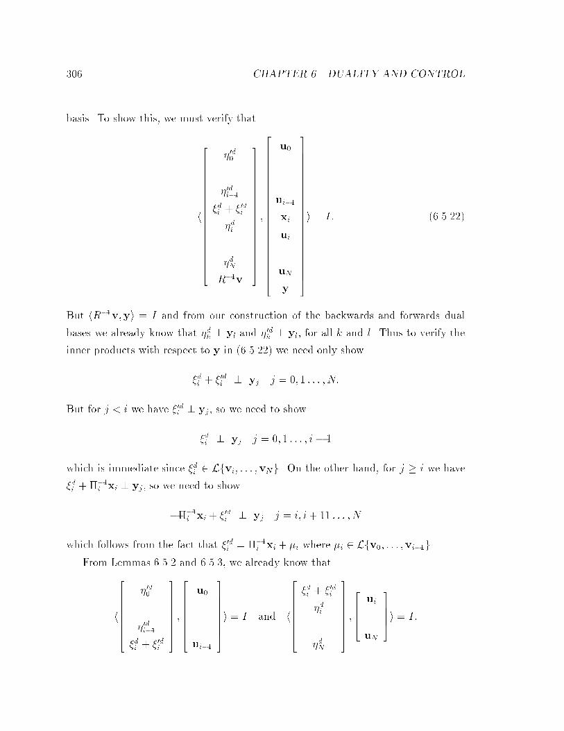
�� CHAPTER �� DUALITY AND CONTROL
basis� To show this� we must verify that
h
���������������������
��d����
��di��
�di � ��di
�di���
�dN
R��v
���������������������
�
�������������������������
u�
���
ui��
xi
ui
���
uN
y
�������������������������
i � I� � ������
But hR��v�yi � I and from our construction of the backwards and forwards dual
bases we already know that �dk � yl and ��dk � yl� for all k and l� Thus to verify the
inner products with respect to y in � ������ we need only show
�di � ��di � yj j � �� � � � � � N�
But for j � i we have ��di � yj� so we need to show
�di � yj j � �� � � � � � i� �
which is immediate since �di � Lfvi� � � � �vNg� On the other hand� for j � i we have
�di �!��i xi � yj� so we need to show
�!��i xi � ��di � yj j � i� i� �� � � � � N
which follows from the fact that ��di � !��i xi � i where i � Lfv�� � � � �vi��g�
From Lemmas ���� and ����� we already know that
h
���������
��d����
��di��
�di � ��di
����������
���������
u�
���
ui��
���������i � I and h
���������
�di � ��di
�di���
�dN
����������
�����ui
���
uN
�����i � I�
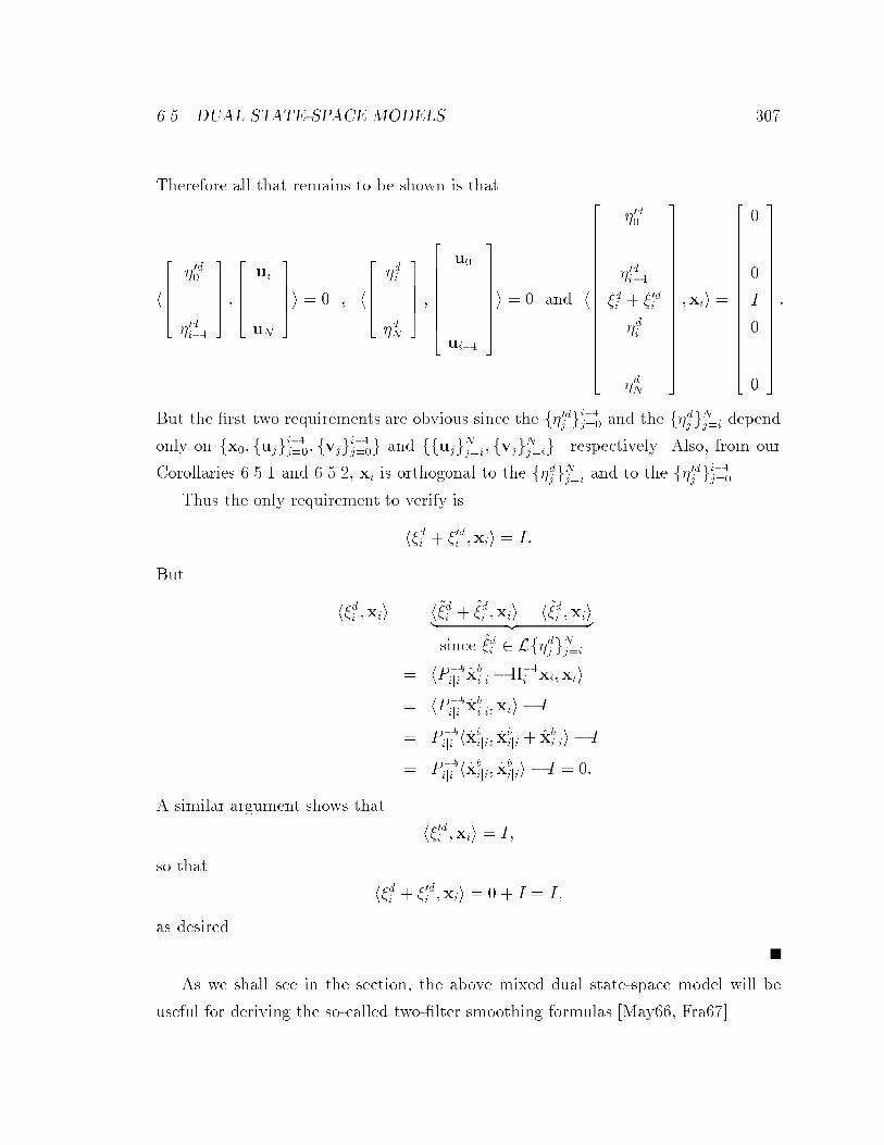
���� DUAL STATE�SPACE MODELS ��
Therefore all that remains to be shown is that
h
�����
��d����
��di��
����� ������ui
���
uN
�����i � � � h
������di���
�dN
����� �
���������
u�
���
ui��
���������i � � and h
������������������
��d����
��di��
�di � ��di
�di���
�dN
������������������
�xii �
������������������
����
�
I
����
�
������������������
�
But the �rst two requirements are obvious since the f��dj gi��j� and the f�dj g
Nji depend
only on fx�� fujgi��j�� fvjg
i��j�g and ffujgNji� fvjg
Njig� respectively� Also� from our
Corollaries ���� and ����� xi is orthogonal to the f�dj gNji and to the f��dj g
i��j��
Thus the only requirement to verify is
h�di � ��di �xii � I�
But
h�di �xii � h��di � ��di �xii � h��di �xii� �z �since ��di � Lf�
dj g
Nji
� hP�biji �x
biji �!��
i xi�xii
� hP�biji �x
biji�xii � I
� P�biji h�x
biji� �x
biji � �xbijii � I
� P�biji h�x
biji� �x
bijii � I � ��
A similar argument shows that
h��di �xii � I�
so that
h�di � ��di �xii � � � I � I�
as desired�
As we shall see in the section� the above mixed dual state�space model will be
useful for deriving the so�called two��lter smoothing formulas �May � Fra ��

��� CHAPTER �� DUALITY AND CONTROL
��� Application to Smoothing
The key observation that allows one to use dual bases for solving smoothing problems
is the following� Suppose we are given a Krein space variable x � Lfz�yg and
would like to �nd� �xjy� the smoothed estimate of x given y� Then since zd is one
possible basis for the orthogonal complement space of Lfyg in Lfz�yg �in other
words� Lfz�yg � Lfyg � Lfzdg�� we may uniquely decompose x as
x � �xjy � �xjzd �
from which it follows
�xjy � x� �xjzd� � � ���
Thus we can obtain the desired estimate by projecting onto the dual basis� zd� and
subtracting the result from x�
The above approach is a general method for obtaining smoothed estimates� Of
course the resulting algorithms will depend on the choice of z �and hence zd�� By
projecting onto the backwards and forwards dual state�space models of Lemmas ����
and ���� it is possible to derive the standard Bryson�Frazier and Rauch�Tung�Striebel
�RTS� smoothing formulae and their variants �RTS ��� The algebra involved in these
derivations is �at times� rather tedious and therefore we shall not present them here�
�The interested reader may refer to �AK��� for details�� Instead� we shall illustrate the
general method by deriving the so�called two��lter smoothing formulae by projecting
onto the mixed dual state�space model of Lemma �����
����� TwoFilter Formulae
Consider the standard state�space model � ����� and suppose that we would like
to obtain� �xijN � the smoothed estimate of the state xi given all the observations
fy�� � � � �yNg� To do so� consider the following mixed dual basis that was introduced
in Lemma �����
f��d� � � � � � ��di��� �
di � ��di � �
di � � � � �
dN � R
��vg� � � ���
To �nd �xijN we will make use of the formula
�xijN�� �xjy � xi � �xijzd� � � ���
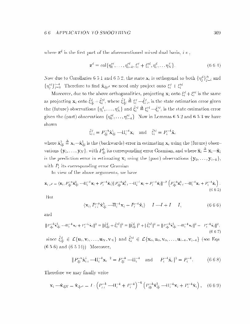
���� APPLICATION TO SMOOTHING ���
where zd is the �rst part of the aforementioned mixed dual basis� i�e��
zd � colf��d� � � � � � ��di��� �
di � ��di � �
di � � � � �
dNg� � � ���
Now due to Corollaries ���� and ����� the state xi is orthogonal to both f�dj gNji and
f��dj gi��j�� Therefore to �nd �xijzd we need only project onto �di � ��di �
Moreover� due to the above orthogonalities� projecting xi onto �di � ��di is the same
as projecting xi onto ��diji����di � where ��diji
�� �di � ��diji� is the state estimation error given
the �future� observations f�di � � � � � �dNg and ���di
�� ��di �
���di � is the state estimation error
given the �past� observations f��d� � � � � � ��di��g� Now in Lemmas ���� and ���� we have
shown
��diji � P�biji �x
biji �!��
i xi and ���di � P��i �xi
where �xbiji�� xi��xbiji is the �backwards� error in estimating xi using the �future� obser�
vations fyi� � � � �yNg� with P biji its corresponding error Gramian� and where �xi
�� xi��xi
is the prediction error in estimating xi using the �past� observations fy�� � � � �yi��g�
with Pi its corresponding error Gramian�
In view of the above arguments� we have
�xijzd � hxi� P�biji
�xbiji ����i xi � P��
i�xiikP
�biji
�xbiji � ���i xi � P��
i�xik
���P�biji
�xbiji � ���i xi � P��
i �xi��
������
But
hxi� P�biji �x
biji �!��
i xi � P��i �xii � I � I � I � I� � � � �
and
kP�biji
�xbiji � ���i xi � P��
i �xik� � k��diji �
���di k� � k��dijik� � k���di k� � kP�b
iji�xbiji � ���
i xik� � kP��
i �xik��
������
since ��diji � Lfui�vi� � � � �uN �vNg and ���di � Lfx��u��v�� � � � �ui���vi��g �see Eqs�
� ��� � and � �������� Moreover�
kP�biji �x
biji �!��
i xik� � P�b
iji �!��i and kP��
i �xik� � P��
i � � � ���
Therefore we may �nally write
xi � �xijN � �xijzd � I �P�biji �!��
i � P��i
��� �P�biji �x
biji �!��
i xi � P��i �xi
�� � � ���

��� CHAPTER �� DUALITY AND CONTROL
or �P�biji �!��
i � P��i
� �xi � �xijN
���P�biji �x
biji �!��
i xi � P��i �xi
�� � � ����
from which we conclude
�P�biji �!��
i � P��i
��xijN � P�b
iji �xbiji � P��
i �xi� � � ����
Computing the Gramian of �xijN from Eq� � � ��� we readily see
PijN ��P�biji �!��
i � P��i
���� � � ����
so that � � ���� becomes
�xijN � PijN
�P�biji �x
biji � P��
i �xi�� � � ����
which is the desired two��lter smoother�
It is left as an exercise to the reader to show that if we had instead begun with
the dual basis
colf��d� � � � � � ��di � �
di � ��di � �
di�� � � � �
dNg � � ����
then we would have obtained the following two��lter formula
�xijN � PijN
�P�bi �xbi � P��
iji �xiji�� � � ����
with
P��ijN �
�P�bi � P��
iji �!��i
���� � � �� �
where �xbi � �xiji� Pbi and Piji have the obvious meanings�
The results are summarized in the following theorem�
Theorem ����� �Two�Filter Smoothing Formulae� Consider the standard state�
space model ������ with the fFig assumed to be invertible� Then we can write
�xijN � PijN �P��i �xi � P�b
iji �xbiji��
with
P��ijN �
�P��i � P�b
iji �!��i
����

��� THE LQR CONTROL PROBLEM ���
or� alternatively�
�xijN � PijN �P��iji �xiji � P�b
i �xbi��
with
P��ijN �
�P��iji � P�b
i �!��i
����
Both sets of formulae require forwards and backwards sweeps over the original data
the �rst formulae require a forwards sweep from y� to yi and a backwards sweep from
yN down to yi�� while the second formulae require a forwards sweep from y� to yi��
and a backwards sweep from yN down to yi�
�� The LQR Control Problem
In this section we shall study the dual problem to Kalman �ltering� i�e� the linear
quadratic regulator �LQR� control problem� The generalization considered here is
that the LQR cost function may be inde�nite �actually problems in H� control
immediately result in such cost functions�� Therefore� contrary to the conventional
case where the problem always had a minimizing solution� we can at most guarantee
a stationarizing solution� Further conditions must be met for the solution to be a
minimum�
The usual method for solving the conventional LQR problem is through a dynamic
programming argument �see e�g� ��BK �� BH ���� Although the dynamic program�
ming principle can be extended from minimizing solutions to include stationarizing
solutions� our approach to solving the LQR problem is similar to the approach we used
for solving H� estimation� we identify a Krein state�space model that corresponds
to the LQR quadratic form �via simple inspection�� and then invoke the Krein space
Kalman �lter to write down the stationarizing solution and its condition for being a
minimum� We should also remark that the Krein space model that most naturally
lends itself to the solution of the LQR control problem is the dual model of Sec� ���
which is what will be used here�
Finally� we should mention that the results of this section will be used to solve
the �nite horizon full information and measurement feedback control problems�

��� CHAPTER �� DUALITY AND CONTROL
���� Problem Formulation
Consider the �possibly� time�varying state�space model
xi� � Fixi �Giui� � � i � N � ����
and some given linear combination of the states
si � Lixi� � ����
where the fui� xig are deterministic quantities� One would like to choose the control
signal ui to regulate the si in a certain sense� The conventional LQR �linear quadratic
regulator� method proposes the following criterion for choosing the ui
minfuig
x�N�PcN�xN� �
NXi�
u�iQciui �
NXi�
s�iRcisi � ����
subject to the state�space constraints � ���� and � ����� where P cN�� Q
ci and Rc
i are
positive�de�nite matrices that penalize the �nal state� the inputs and the intermediary
states� respectively�
In many applications� such as the H� problems to be studied� one needs to con�
sider the quadratic form in � ���� when the P cN�� Q
ci and R
ci are inde�nite Hermitian
matrices� Therefore� let us introduce the notation for the quadratic form in � ���� as
J cN�x�� u�� � � � � uN� � x�N�P
cN�xN� �
NXi�
u�iQciui �
NXi�
s�iRcisi� � ����
where from now on we shall drop the positivity conditions on the P cN�� Q
ci and Rc
i �
Since J cN will now be an inde�nite quadratic form� it does not necessarily have a
minimum over the fuig� and the most that we can guarantee is a stationary point�
With this in mind� we may now state the �nite horizon LQR control problem as
follows�
Problem ����� �Finite Horizon LQR Control Problem� Find the control sig�
nals f�uigNi� that stationarize the quadratic form
J cN �x�� u�� � � � � uN� � x�N�P
cN�xN� �
NXi�
u�iQciui �
NXi�
s�iRcisi

��� THE LQR CONTROL PROBLEM ���
subject to the state�space relations ������ and �������� where by a stationary point we
meanJ c
N
ui�x�� �u�� � � � � �uN� � �� � � i � N�
Moreover� �nd the necessary and su�cient conditions for this stationary point to be
a minimum�
���� Solution Based on Duality
Let us begin by de�ning u � colfu�� � � � � uNg and s � colfs�� � � � � sNg� so that we may
use the state equation � ���� and the output equation � ���� to write
xN� � #Fx� � Cu and y � Ox� � " � ����
where #F � FNFN�� � � � F� is the state transition matrix�
O �
���������
L�
L�F����
LNFN�� � � � F�
����������
is the observability map�
C �hFNFN�� � � � F�G� FNFN�� � � � F�G� � � � G�
i�
is the controllability map� and
" �
������������
�
H�G� �
H�F�G� H�G�
������
� � �
HNFN�� � � � F�G� HNFN�� � � � F�G� � � � HNGN��
�������������
is the impulse response matrix� If we further de�ne�
Qc � diagfQc�� Q
c�� � � � � Q
cNg and Rc � diagfRc
�� Rc�� � � � � R
cNg�

��� CHAPTER �� DUALITY AND CONTROL
then we can write the LQR cost function� J cN � as a quadratic form in terms of x� and
u� We thus have
J cN � �x��#
�F � u�C��P c
N��#Fx� � Cu� � �x��O� � u�"��Rc�Ox� � "u� � u�Qcu�
or� after gathering terms�
J cN �
hx�� u�
i �� #�FP
cN�#F �O�RcO #�
FPcN�C �O�Rc"
C�P cN�#F � "�RcO C�P c
N�C � "�Rc" �Qc
���� x�
u
�� �� �� �
Now if we de�ne ��� xc� � #�
FxcN� �O�uc
yc � C�xcN� � "�uc � vc� ���
where xcN�� uc and vc are Krein space variables with
h
�����xcN�
uc
vc
����� ������xcN�
uc
vc
�����i �
�����P cN� � �
� Rc �
� � Qc
����� �
then it is straightforward to see that
h
�� xc�
yc
�� ��� xc�
yc
��i �
�� #�
FPcN�#F �O�RcO #�
FPcN�C �O�Rc"
C�P cN�#F � "�RcO C�P c
N�C � "�Rc" �Qc
�� � � ����
so that the LQR cost function in � �� � can be rewritten as
J cN �
hx�� u�
i�� Rxc�
Rxc�yc
Rycxc�
Ryc
���� x�
u
�� � � ����
The minimizing solution over u for J cN is now readily seen to be
�u � �R��yc Rycxc
�x�� � �����
i�e�� its gain matrix �R��yc Rycxc
�is the negative �conjugate� transpose of the gain
matrix in estimating the random variable xc� from yc� Note that this is the dual
stochastic approach to deterministic least�squares problems that was introduced in
Sec� ��� Therefore to �nd our desired solution we can project xc� onto yc and use
the negative �conjugate� transpose of the resulting gain matrix to �nd �u�

��� THE LQR CONTROL PROBLEM ���
To this end� let us �rst note that � ��� has the following backwards dual state�
space model ��� xci � F �
i xci� � L�iu
ci � xcN�
yci � G�
ixci� � vc
i
� �����
with
h
�����
uci
vci
xcN�
����� ������
ucj
vcj
xcN�
�����i �
�����Rc
i�ij � �
� Qci�ij �
� � P cN�
����� �
as can be readily checked by de�ning yc � colfyc�� � � � �y
cNg� u
c � colfuc�� � � � �u
cNg and
vc � colfvc�� � � � �v
cNg� noting the relations
xc� � #�Fx
cN� �O�uc � yc � C�xcN� � "�uc � vc � �����
and computing the respective Gramians�
To �nd the projection of xc� onto yc we can invoke the Krein space Kalman �lter
corresponding to � ������ Thus
�xci � F �i �x
ci� �Kc
p�ieci � �xcN� � � � �����
where
eci � yci �G�
i �xci�� � �����
is the innovations�
Kcp�i � F �
i Pci�Gi�R
ce�i�
�� and Rce�i � Qc
i �G�iP
ci�Gi � �����
are the Kalman gain and innovations variance� respectively� and where P ci satis�es
the backwards�time Riccati recursion
P ci � F �
i Pci�Fi � L�iR
ciLi �Kc
p�iRce�iK
c�p�i� P c
N�� � ��� �
Now � ����� may be rewritten as
�xci � #i�xci� �Kc
p�iyci � �xcN� � � � ����
where
#i � �F �i �Kc
p�iG�i ��

�� CHAPTER �� DUALITY AND CONTROL
The recursion � ���� can be solved to yield
�xc� �hKc
p�� #�Kcp�� � � � #� � � �#N��K
cp�N
i���������
yc�
yc�
���
ycN
���������� � �����
Now the solution to the LQR problem is given by the negative of the conjugate
transpose of the above solution� Thus���������
�u�
�u����
�uN
���������� �
���������
Kc�p��
Kc�p��#
��
���
Kc�p�N#
�N�� � � �#
��
���������x�� � �����
But this implies
�u� � �Kc�p���
and
�u� � �Kc�p��#
�� � �Kc�
p���F� �G�Kc�p���x�
� �Kc�p���F�x� �G��u�� � �Kc�
p��x��
and continuing in a similar fashion
�ui � �Kc�p�ixi� i � �� � � � � N � �����
which is the wellknown state�feedback law of LQR control�
Equations � ������ � ��� � and � ����� constitute the solution to the LQR control
problem� Of course� we still need to check the condition for a minimumover� the fuig�
But� using Lemma ����� this is readily seen to be
Ryc � C�P cN�C � "�Rc" �Qc � �� � �����
Moreover� the Krein space Kalman �lter corresponding to Ryc allows us to recursively
check the above condition via the innovations Gramian� viz��
Rce�i � Qc
i �G�iP
ci�Gi � �� i � �� � � � � N� � �����

��� THE LQR CONTROL PROBLEM ��
Now the control signal� �u � �R��yc Rycxc
�x�� is referred to as the optimal open�loop
control� since it only depends on the initial state� x�� The control signal� �ui � �Kc�p�ixi�
on the other hand� is referred to as the optimal closed�loop control� since it depends
only on the current state� xi� Note that at any given time� i� the optimal closed�loop
control signal� �ui � �Kc�p�ixi� coincides with the optimal open�loop signal if� and only
if� all previous choices of the control signal were also optimal� �Since non�optimal
choices of fuj� j � ig a�ect the value of xi� and thereby the value of the optimal
closed�loop control� �ui � �Kc�p�ixi��
The closed�loop control signal� however� has the additional property that it is the
optimal control at time i� irrespective of what the previous control signals were� To
be more speci�c� it solves the LQR problem�
minui
NXji
u�jQcjuj �
NXji
s�jRcjsj � x�N�P
cN�xN�� � �����
The validity of the above claim is readily seen from the fact that in the above ar�
gument� which led to the optimal choice of u�� i�e�� �u� � �Kc�p��x�� the choice of the
initial time� i � �� was arbitrary�
The closed�loop control signals� �ui � �Kc�p�ixi� also allow for a certain decomposi�
tion of the LQR cost� which will prove to be extremely useful� Indeed��
J cN�x�� u�� � � � � uN� � x��P
c�x� �
NXj�
�uj � �uj��Rc
e�j�uj � �uj�� � �����
We can now summarize the results obtained so far in the following Theorem�
where� to conform with the results of Sec� ������ we have de�ned� Kc�i�� Kc�
p�i�
�This identity can be shown in several di�erent ways� One way is to complete the squares in theexpression for JcN � ������� to write
JcN � x��Pc�x� � u� R��
yc Rycxc�x��
�Ryc u�R��yc Rycxc
�x���
The triangular decomposition� Ryc � L�RecL� obtained from the Krein space Kalman �lter forRyc� can then after some amount of algebra� be used to show the desired result� A shorter proof isto repeatedly apply the readily veri�ed via completion of squares� identity�
u�jQcjuj � s�jR
cjsj � x�j��P
cj��xj�� � x�jP
cj xj � uj � �uj�
�Rce�j uj � �uj��
to the quadratic form� JcN �

��� CHAPTER �� DUALITY AND CONTROL
Theorem ����� �Finite Horizon LQR Solution� Consider the LQR cost func�
tion
J cN�x�� u�� � � � � uN � � x�N�P
cN�xN� �
NXi�
u�iQciui �
NXi�
s�iRcisi�
with P cN�� Q
ci � and R
ci � given Hermitian matrices� and suppose that we want to mini�
mize J cN�x�� u�� � � � � uN � over the variables fuig
Ni� subject to the state�space constraint
xi� � Fixi �Giui� i � �� � � � � N � Then the minimizing solution is given by the state�
feedback law
�ui � �Kc�ixi� i � �� � � � � N � �����
where
Kc�i � F �i P
ci�Gi�R
ce�i�
�� � ��� �
and
Rce�i � Qc
i �G�iP
ci�Gi � ����
and where P ci satis�es the backwards�time Riccati recursion
P ci � F �
i Pci�Fi �H�
i RciHi �Kc�iR
ce�iK
�c�i� P c
N�� � �����
The condition for the above solution to be a minimum is that
Rce�i � �� i � �� � � � � N� � �����
Moreover� we have the identity�
J cN�x�� u�� � � � � uN� � x��P
c�x� �
NXj�
�uj � �uj��Rc
e�j�uj � �uj�� � �����
Remark� Note that we obtained the solution to the LQR problem by appealing to
the dual approach for solving deterministic least�squares problems� The solution was
obtained by constructing the Kalman �lter for the backwards�time dual state�space
model� This� therefore� directly suggests the wellknown duality between Kalman
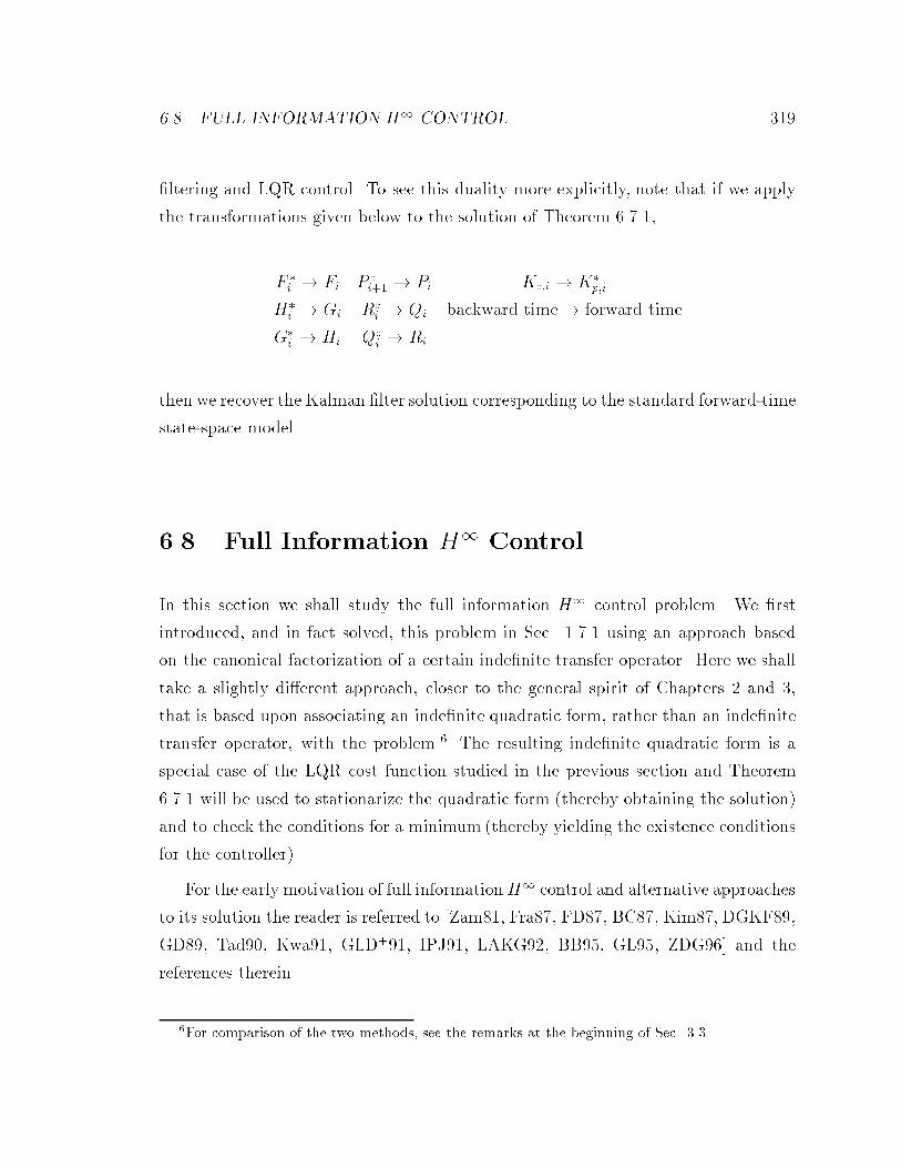
��� FULL INFORMATION H� CONTROL ���
�ltering and LQR control� To see this duality more explicitly� note that if we apply
the transformations given below to the solution of Theorem ����
F �i � Fi P c
i� � Pi Kc�i � K�p�i
H�i � Gi Rc
i � Qi backward time� forward time
G�i � Hi Qc
i � Ri
then we recover the Kalman �lter solution corresponding to the standard forward�time
state�space model�
�� Full Information H Control
In this section we shall study the full information H� control problem� We �rst
introduced� and in fact solved� this problem in Sec� ���� using an approach based
on the canonical factorization of a certain inde�nite transfer operator� Here we shall
take a slightly di�erent approach� closer to the general spirit of Chapters � and ��
that is based upon associating an inde�nite quadratic form� rather than an inde�nite
transfer operator� with the problem�� The resulting inde�nite quadratic form is a
special case of the LQR cost function studied in the previous section and Theorem
��� will be used to stationarize the quadratic form �thereby obtaining the solution�
and to check the conditions for a minimum �thereby yielding the existence conditions
for the controller��
For the early motivation of full informationH� control and alternative approaches
to its solution the reader is referred to �Zam��� Fra�� FD�� BC�� Kim�� DGKF���
GD��� Tad��� Kwa��� GLD��� IPJ��� LAKG��� BB��� GL��� ZDG� � and the
references therein�
�For comparison of the two methods� see the remarks at the beginning of Sec� ����

��� CHAPTER �� DUALITY AND CONTROL
����� Problem Formulation
Consider the �possibly� time�variant state�space model
xi� � Fixi �G��iwi �G��iwi
� Fixi �hG��i G��i
i �� wi
ui
�� i � �� � � �N� � �����
where the fuig are the control inputs� and x� and the fwig are deterministic dis�
turbances� The fwig may be interpreted as process noise or driving disturbance�
Consider a given linear combination of the states�
si � Lixi� � �����
that we intend to regulate using the control signal ui� In the full information problem�
it is assumed that that the control signal� ui� has access to current and past values of
the disturbances� fx�� w�� � � � � wig� Let
$ui � Fi�x�� w�� � � � � wi�� � �����
denote a such a full information control strategy�
Using this control strategy� let T �F� denote the transfer operator that maps the
disturbances �!� �
�
� x�� f�Qwi �
�
�wigNi�
��
to the variables n�P c
N���
�xN�� f�Qci�
�
� $uigNi�� f�R
ci �
�
� sigNi�
o�
where !�� P cN�� Q
wi � Q
ci and Rc
i are positive �semi�de�nite weighting matrices� The
�nite horizon full information H� control problem can now be stated as follows�
Problem ����� �Optimal Full Information H� Control Problem� Find a ��
nite horizon full information H��optimal control strategy $ui � Fi�x�� w�� � � � � wi� that
minimizes T �F� and obtain the resulting
��opt � infFk T �F� k��� inf
Fsup
x��w�h�
x�N�PcN�xN�� k �Qc
i��
� $ui k� � k �Rci �
�
� si k�
x�!��� x�� k �Qw
i ��
�wi k��
� �����

��� FULL INFORMATION H� CONTROL ���
Note that the numerator in � ����� is simply the LQR cost function� Thus the
above problem formulation guarantees the smallest LQR cost over all possible distur�
bances of �xed energy� H� controllers must therefore accommodate for all conceivable
disturbances� which re%ects in better robust behaviour with respect to disturbance
variation�
A closed form solution to the optimal full information H� control problem is
available only for some special cases� and a simpler problem results if one relaxes the
minimization condition and settles for a suboptimal solution�
Problem ����� �Suboptimal H� Problem� Find a suboptimal full information
H� control strategy $ui � Fi�x�� w�� � � � � wi� that achieves k T �F� k�� �� This
clearly requires checking whether � � �opt�
����� Solution
Before giving the solution to the full informationH� control problem� it will be useful
to study the structure of the problem in slightly more detail� In view of Prob� �����
we must �nd a control strategy $ui � Fi�x�� w�� � � �wi� such that
supx��w�h�
x�N�PcN�xN�� k �Qc
i��
� $ui k� � k �Rci �
�
� si k�
x�!��� x�� k �Qw
i ��
�wi k�� ���
or� in other words� a control strategy� such that for all nonzero x� and fwigNi��
x�N�PcN�xN� �
PNi� $u
�iQ
ci $ui �
PNi� s
�iR
cizi
x�!��� x� �
PNi� w
�iQ
wi wi
� ��� � �����
Multiplying � ����� by the nonzero denominator� we obtain the following result�
Lemma ����� �Full Information H� Control and Quadratic Forms� Given a
scalar � � �� there exists a full information controller that achieves k T �F� k�� � if�
and only if� there exists $ui � Fi�x�� w�� � � � wi� �for all i � �� � � � � N� such that for all
nonzero complex vectors x� and all nonzero sequences fwigNi�� the scalar quadratic
form
J cN � x��!
��� x� � ����x�N�P
cN�xN� �
NXi�
$u�iQci $ui � ��
NXi�
w�iQ
wi wi �
NXi�
s�iRcisi�

��� CHAPTER �� DUALITY AND CONTROL
� x��!��� x� � ����x�N�P
cN�xN� �
NXi�
h$u�i w�
i
i�� Qci �
� ���Qwi
���� $ui
wi
���
NXi�
s�iRcisi�
satis�es
J cN � ��
The quadratic form appearing in the parentheses of J cN is simply the LQR cost
function associated with the state�space model � ������ and with weighting matrices
PN��
�� Qc
i �
� ���Qwi
��� and Rc
i � respectively� Note that one of the weighting matrices
is inde�nite� which is why we considered the Krein space setting in Sec� �� We may
thus use Eq� � ����� of Theorem ��� to rewrite J cN as
J cN � x��!
��� x� � ��� �x��P
c�x��
PNi�
�� $ui � �ui
wi � �wi
����� Qc
i �G���iP
ci�G��i G�
��iPci�G��i
G���iP
ci�G��i ���Qw
i �G���iP
ci�G��i
���� $ui � �ui
wi � �wi
���A �
� ��� �
where �ui and �wi are given by �� �ui
�wi
�� � �Kc�ixi� � ����
with
Kc�i � �Rce�i�
��
�� G�
��i
G���i
��P c
i�Fi� � �����
where
Rce�i �
�� Qc
i �G���iP
ci�G��i G�
��iPci�G��i
G���iP
ci�G��i ���Qw
i �G���iP
ci�G��i
�� � � �����
and where P ci satis�es the backwards Riccati recursion
P ci � F �
i Pci�Fi � L�iR
ciLi �K�
c�iRce�iKc�i� P c
N�� � ������
In order to solve the full information problem� let us introduce the following block
LDU factorization of Rce�i��
� Im��
G���iP
ci�G��iR
��Gc �i Im�
���� RGc�i �
� &i
���� Im�
R��Gc �iG
���iP
ci�G��i
� Im�
�� � � ������
��� FULL INFORMATION H� CONTROL ���
where we have de�ned
RGc�i�� Qc
i �G���iP
ci�G��i� � ������
and the Schur complement�
&i�� ���Qw
i �G���iP
ci�G��i �G�
��iPci�G��iR
��Gc�iG
���iP
ci�G��i� � ������
The factorization in � ������ allows us to write J cN as
J cN � x���!
��� ����P c
� �x�����
NXi�
�$ui�'ui��RGc�i�$ui�'ui���
��NXi�
�wi� �wi��&i�wi� �wi��
� ������
where we have de�ned 'ui via�� $ui � 'ui
wi � �wi
�� �
�� Im�
�
G���iP
ci�G��iR
��Gc�i Im�
���� $ui � �ui
wi � �wi
�� � � ������
so that� after some algebraic simpli�cation� we obtain
'ui � �R��Gc�iG
���iP
ci�Fixi �R��
Gc�iG���iP
ci�G��iwi� � ���� �
Note that 'ui is a function of fx�� w�� � � � � wig� whereas �ui and �wi are functions of
fx�� w�� � � � � wi��g�
Referring back to Eq� � ������ we see that since $ui is only allowed to be a function
of fx�� w�� � � � � wig it cannot in%uence the �rst and third terms in the summation for
J cN �
Thus a necessary condition for J cN to be positive for all nonzero fx�� w�� � � � wNg
is that the �rst and third terms be positive for all such disturbances� In other words�
if
!��� � ���P c
� � �� � �����
and
&i � �� i � �� � � � N� � ������
The above conditions are also su�cient� since we can always choose the control signal
to be�
$ui � 'ui� � ������
To see why� note that x�� ���� ����P c
� �x� is independent of �ui� and� moreover� that the controllercannot in�uence the value of wi� �wi���i wi� �wi� since �wi depends only on previous controls whichhave no knowledge of wi�

��� CHAPTER �� DUALITY AND CONTROL
which yields� incidentally� the central controller�
We have thus established the following result�
Theorem ����� �Finite�Horizon Full Information H� Control� Consider the
state�space model ������ and de�ne T �F� as the transfer operator that maps the dis�
turbances f!� �
�
� x�� f�Qwi �
�
�wigNi�g to the variables f�PcN��
�
�xN�� f�Qci�
�
� $ui� �Rci �
�
� sigNi�g�
where !�� P cN�� Q
wi � Q
ci and R
ci are positive �semi�de�nite weighting matrices� Then
for any given � � �� a full information H� control strategy� $ui � Fi�x�� w�� � � � � wi��
that yields
k T �F� k�� ��
exists if� and only if�
�i� !��� � ���P c
� � �
�ii� &i � ���Qwi �G�
��iPci�G��i �G�
��iPci�G��iR
��Gc �iG
���iP
ci�G��i � � i � �� � � � � N
where RGc�i � Qci �G�
��iPci�G��i� and P c
i� satis�es the backwards Riccati recursion
P ci � F �
i Pci�Fi � L�iR
ciLi �Kc� i�Rc
e�iKc�i� P cN�
with
Kc�i � �Rce�i�
��
�� G�
��i
G���i
��P c
i�Fi�
and
Rce�i �
�� Qc
i �G���iP
ci�G��i G�
��iPci�G��i
G���iP
ci�G��i ���Qw
i �G���iP
ci�G��i
�� �
If this is the case� then all possible full information H� control strategies� $ui �
Fi�x�� w�� � � � � wi�� are given by those that satisfy�
x���!��� ����P c
� �x�����NXi�
�$ui� 'ui��RGc �i�$ui� 'ui�����
NXi�
�wi� �wi��&i�wi� �wi� � ��
where �wi is de�ned via� �� �ui
�wi
�� � �Kc�ixi�

��� FULL INFORMATION H� CONTROL ���
and 'ui� via
'ui � �R��Gc�iG
���iP
ci�Fixi �R��
Gc�iG���iP
ci�G��iwi�
Finally� the so�called central controller is given by�
$ui � 'ui� � ������
Remarks�
�i� Note that the above Theorem is simply the �nite�horizon time�variant counter�
part of Theorem ����� �See also the comments at the end of Sec� ������
�ii� The solution to the H� control problem with perfect state measurement� as
given by Theorem ����� is a special case of the LQR control problem studied
in Sec� �� Note that we needed the Krein space extension of the LQR theory
�with inde�nite weighting matrices� since the H� control problem leads to such
types of cost functions�
�iii� There are two conditions for the existence of H� controllers� one is a certain
positivity check for the solution of the backwards Riccati at each time instant�
and one is a coupling condition between the end�point solution of the Riccati
and the weighting on the initial state x�� This last condition is reminiscent
of the separation principle and coupling condition that occurs in measurement
feedback H� control� which we shall study in the next section�
�iv� The central full information controllers given by Eq� � ������ have the same
basic properties that the central �lters of H� estimation had� In other words�
they are risk�sensitive optimal with risk�sensitivity parameter� � � ����� they
are the solution to certain quadratic dynamic games� and they are maximum
entropy controllers�
�v� We should mention that the central control law � ����� is not exactly a state
feedback law �as happens in continuous�time full information H� control� since

�� CHAPTER �� DUALITY AND CONTROL
the second term involves wi� The reason is� of course� that we have allowed
the control signal to be a causal function of the disturbances� i�e�� a function of
fx�� w�� � � �wig� If we restrict the control signal to be a strictly causal function
of the disturbances� i�e�� a function of fx�� w�� � � �wi��g� then� as shown below�
we do obtain a state feedback law for the central controller� �Compare with the
remarks following Theorem ������
When the control signal is restricted to be a strictly causal function of the dis�
turbances� i�e�� $ui � Fi�x�� w�� � � �wi���� then the only di�erence in the arguments
preceding Theorem ���� is that we need to replace the block LDU factorization
� ������ of Rce�i with its block upper�diagonal�lower �UDL� factorization�
�� Im�
G���iP
ci�G��i�R
�
Gc�i���
� Im�
���� &
�
i �
� R�
Gc�i
���� Im�
�
�R�
Gc�i���G�
��iPci�G��i Im�
�� �
� ������
where we have de�ned
R�
Gc�i
�� ���Qw
i �G���iP
ci�G��i� � ������
and the Schur complement�
&�
i
�� Qc
i �G���iP
ci�G��i �G�
��iPci�G��i�R
�
Gc�i���G�
��iPci�G��i� � ������
The factorization in � ������ allows us to write J cN as
J cN � x���!
��� ����P c
� �x�����
NXi�
�$ui��ui��&
�
i�$ui��ui�����
NXi�
�wi� 'wi��R
�
Gc�i�wi� 'wi��
� ������
where 'wi is de�ned via��� $ui � �ui
wi � 'wi
�� �
�� Im�
G���iP
ci�G��i�R
�
Gc�i���
� Im�
���� $ui � �ui
wi � �wi
�� � � ������
Note that since ui is only a function of �x�� w�� � � � wi���� it can only e�ectively in%u�
ence the second term in the summation for J cN in Eq� � ������� Therefore proceeding
with an argument similar to the one that led to the proof of Theorem ����� we obtain
the following result�

��� FULL INFORMATION H� CONTROL ��
Theorem ����� �Strictly Causal Full Information H� Control� Consider the
state�space model ������ and de�ne T �F� as the transfer operator that maps the dis�
turbances f!� �
�
� x�� f�Qwi �
�
�wigNi�g to the variables f�PcN��
�
�xN�� f�Qci�
�
� $ui� �Rci �
�
� sigNi�g�
where !�� P cN�� Q
wi � Q
ci and R
ci are positive �semi�de�nite weighting matrices� Then
for any given � � �� a strictly causal full information H� control strategy� $ui �
Fi�x�� w�� � � � � wi���� that yields
k T �F� k�� ��
exists if� and only if�
�i� !��� � ���P c
� � �
�ii� R�
Gc�i � ���Qwi �G�
��iPci�G��i � � i � �� � � � � N
where P ci� is the same as in Theorem ����� If this is the case� then all possible
strictly causal full information H� control strategies� $ui � Fi�x�� w�� � � � � wi���� are
given by those that satisfy�
x���!��� ����P c
� �x�����NXi�
�$ui� �ui��&
�
i�$ui� �ui�����NXi�
�wi� 'wi��R
�
Gc �i�wi� 'wi� � ��
where &�
i � Qci �G�
��iPci�G��i �G�
��iPci�G��i�R
�
Gc �i���G�
��iPci�G��i� and where
'wi � ��R�
Gc�i���G�
��iPci�Fixi � �R
�
Gc�i���G�
��iPci�G��i$ui� � ���� �
and
�ui � ��Qci �G�
��i�P ci�G��i�
��G���i
�P ci�Fixi� � �����
with
�P ci� � P c
i� � P ci�G��i�R
�
Gc �i���G�
��iPci�� � ������
Finally� the so�called central controller is given by�
$ui � �ui� � ������

��� CHAPTER �� DUALITY AND CONTROL
��� Measurement Feedback H Control
In this section we shall study the �nite horizon H� control problem with measure�
ment feedback� We �rst introduced� and in fact solved� this problem in Sec� �����
The approach used there was based on a certain separation principle that reduced
the measurement feedback problem to two coupled problems� one a full information
control problem� and one an estimation problem �essentially for estimating the un�
observable full information control signals using the available measurements�� The
approach taken here is the same� and is a direct application of our earlier results
on H� �ltering �from Chapter �� and full information H� control �from Sec� ����
coupled with the aforementioned separation principle� We should mention that the
separation principle presented here is slightly di�erent from the separation principles
�rst presented in H� control �DGKF��� and risk�sensitive control �Whi���� and is
closer to the separation principle given in �GL���� We should also mention� however�
as pointed out earlier in Remark �i� following Theorem ����� that the two separation
principles are closely related� although we believe that the one presented here is more
natural since it does not need to appeal to state�space models�
����� Problem Formulation
Consider the �possibly� time�variant state�space model
���������xi� � Fixi �G��iwi �G��iui
yi � Hixi � vi
si � Lixi
i � �� � � � N� � �����
where the fuig are the control inputs� the fx�� fwig� fvigg are unknown disturbances�
the fyig are the observed outputs� and the fsig are the signals we intend to regulate�
The fwig may be interpreted as process noise and the fvig as measurement noise�
Moreover let $ui be a control strategy that uses current and past observations� i�e�
$ui � Fi�y�� � � � � yi��
With this control strategy� let T �F� denote the transfer operator that maps the

���� MEASUREMENT FEEDBACK H� CONTROL ���
unknown disturbances
�!� ��
� x�� f�Qwi �
�
�wigNi�� f�R
vi �� �� vig
Ni�
��
to the variables n�P c
N���
�xN�� f�Rci �
�
� sigNi�� f�Q
ci�
�
� $uigNi�
o�
where !�� P cN�� Q
wi � Q
ci R
vi and Rc
i are positive �semi�de�nite weighting matrices�
The H� control problem with output feedback can now be stated as follows� �See
�gure ����
P P
P P
11 12
21 22
w s
u
v
y
i
i
i
i
i
t i
F
Figure ��� H� control with measurement feedback�
Problem ����� �Optimal Measurement Feedback H� Control Problem� Find
a �nite horizon H��optimal measurement feedback control strategy $ui � Fi�y�� � � � � yi�
that minimizes T �F� and obtain the resulting
��opt � infFk T �F� k��� inf
Fsup
x��w�h��v�h�
x�N�PcN�xN�� k �Qc
i��
� $ui k� � k �Rci �
�
�Lixi k�
x�!��� x�� k �Qw
i ��
�wi k� � k �Rvi �� �� vi k�
�
� �����
��� CHAPTER �� DUALITY AND CONTROL
Note that the numerator in � ����� is simply the LQR cost function� Thus� as
before� the above problem formulation guarantees the smallest LQR cost over all pos�
sible disturbances of �xed energy� The resultingH� controllers are thus conservative�
which re%ects in a better robust behaviour with respect to disturbance variation�
As we have seen earlier� closed form solutions to the optimal H� problem are
available for only some special cases� We therefore obtain a simpler problem if we
relax the minimization condition and settle for a suboptimal solution�
Problem ����� �Suboptimal H� Problem� Find a suboptimal measurement feed�
back H� control strategy $ui � Fi�y�� � � � yi� that achieves k T �F� k�� �� This clearly
requires checking whether � � �opt�
����� Solution
We begin by examining the structure of the problem in slightly more detail� In view
of Prob� ����� we must �nd a control strategy $ui � Fi�y�� � � � � yi� such that
supx��w�h��v�h�
x�N�PcN�xN�� k �Qc
i��
� $ui k� � k �Rci �
�
�Lixi k�
x�!��� x�� k �Qw
i ��
�wi k� � k �Rvi �� �� vi k�
� ���
or� in other words� a control strategy� such that for all nonzero x�� fvigNi� and fwig
Ni��
x�N�PcN�xN� �
PNi� $u
�iQ
ci $ui �
PNi� x
�iLi �Rc
iLixi
x�!��� x� �
PNi�w
�iQ
wi wi �
PNi� v
�i �R
vi ���vi
� ��� � �����
Multiplying � ����� by the nonzero denominator� we obtain the following result�
Lemma ����� �Measurement Feedback H� Control and Quadratic Forms�
Given a scalar � � �� there exists a measurement feedback controller that achieves
k T �F� k�� � if� and only if� there exists $ui � Fi�y�� � � � � yi� �for all i � �� � � � � N�
such that for all nonzero complex vectors x�� and all nonzero sequences fvigNi� and
fwigNi�� the scalar quadratic form
JmN � x��!
��� x� �
NXi�
w�iQ
wi wi �
NXi�
�yi �Hixi���Rv
i ����yi �Hixi��
����NXi�
x�iL�iR
ciLixi �
NXi�
$u�iQci $ui � x�N�P
cN�xN���

���� MEASUREMENT FEEDBACK H� CONTROL ���
satis�es
JmN � ��
In other words if� and only if�
�i� JmN �x�� w�� � � � � wN � $u�� � � � � $uN� has a minimum over fx�� w�� � � � � wNg�
�ii� The f$u�� � � � � $uNg can be chosen such that the value of JmN at this minimum be
positive�
The above Lemma requires us to minimize JmN over the variables� fx�� w�� � � � � wNg
and to compute its value at this minimum� Since the expression for JmN is quite
complicated� this appears to be a formidable task� To somewhat alleviate the problem�
let us reorganize JmN in the following fashion�
JmN � x��!
��� x� �
NXi�
�yi �Hixi���Rv
i ����yi �Hixi�
����
�� NXi�
x�iL�iR
ciLixi �
NXi�
�� wi
$ui
����� ���Qw
i �
� Qci
���� wi
$ui
��� x�N�P
cN�xN�
�� �
Note that the expression inside the brackets is simply the inde�nite quadratic form
associated with the full information problem� �See Lemma ������ Therefore we can
use Eq� � ��� � to write it as
x��Pc�x� �
NXi�
�� wi � �wi
$ui � �ui
��� �Rc
e�i���
�� wi � �wi
$ui � �ui
�� � � �����
where �wi and �ui are given by
�� �wi
�ui
�� � �Kc�ixi
�� �
�� Kw�i
Ku�i
��xi� � �����
with
Kc�i � �Rce�i�
��
�� G�
��i
G���i
��P c
i�Fi� � ��� �

��� CHAPTER �� DUALITY AND CONTROL
where
Rce�i �
�� ���Qw
i �G���iP
ci�G��i G�
��iPci�G��i
G���iP
ci�G��i Qc
i �G���iP
ci�G��i
�� � � ����
and where P ci satis�es the backwards Riccati recursion
P ci � F �
i Pci�Fi � L�iR
ciLi �K�
c�iRce�iKc�i� P c
N�� � �����
Now Eq� � ����� allows us to write JmN as follows�
JmN � x���!
��� � ���P c
� �x� �
NXi�
�����
wi � �wi
$ui � �ui
yi �Hixi
������ ����� ��
��
�� Rc
e�i��� �� Rce�i��� ��
Rce�i��� �� Rc
e�i��� ��
�� �
� �Rvi ���
����������
wi � �wi
$ui � �ui
yi �Hixi
����� �
where the Rce�i�i� j� denote the �obvious� block entries of Rc
e�i� Now if we de�ne��� &��
i'Si
'S�i �&�
i���
�� ��
�� Rc
e�i��� �� Rce�i��� ��
Rce�i��� �� Rc
e�i��� ��
�� � � �����
then JmN can be written as�
JmN � x���!
��� ����P c
� �x��NXi�
�����
wi � �wi�� $ui
yi
���
�� Ku�i
Hi
�������� �� Qi Si
S�i Ri
����
�����
wi � �wi�� $ui
yi
���
�� Ku�i
Hi
������� �
� ������
where we have de�ned�
Qi�� ���&��
i � Si�� ���
h'Si �
i� Ri
��
�� ���&
�
i��� �
� Rvi
�� � � ������
But note that JmN � as given by � ������� is now the standard estimation quadratic
form of Sec� �� �see Eq� ��� ���� for the Krein space state�space model�����������
xi� � �Fi �G��iKw�i�xi �G��i�wi � �wi� �G���$ui�� $ui
yi
�� �
�� �Ku�i
Hi
��xi � vi
� � ������
Note that we have used �wi � �Kw�ixi to rewrite the state equation as
xi�� � Fixi �G��iwi �G����ui � Fi �G��iKw�i�xi � G��i wi � �wi� � G����ui�
���� MEASUREMENT FEEDBACK H� CONTROL ���
with
h
�����
x�
wi � �wi
vi
����� ������
x�
wj � �wj
vj
�����i �
�����
�!��� � ���P c
� ��� �
�
�� Qi Si
S�i Ri
�� �ij
����� � � ������
We can now use the results of Theorem ���� and Lemma ���� to minimize JmN over
the variables� fx�� w�� � � � wNg and to check the conditions for a minimum� Note that
the condition for a minimum is that�
�i� !��� � ���P c
� � �
�ii� Qi � ���&��i � �� for all j � �� � � � � N
�iii� Ri � S�Q��i S and Re�i have the same inertia� for all j � �� � � � � N
where
Re�i � Ri �
�� �Ku�i
Hi
��Pi
h�K�
u�i H�i
i� � ������
and Pi satis�es the Riccati recursion�
Pi� � �Fi �G��iKw�i�Pi�Fi �G��iKw�i�� ����G��i&
��i G�
��i �Kp�iRe�iK�p�i� � ������
initialized with P� � �!��� � ���P c
� ���� and with
Kp�i �n�Fi �G��iKw�i�Pi
h�K�
u�i H�i
i�G��iSi
oR��
e�i � � ���� �
Now some simple algebra shows that
Ri � S�Q��i S �
�� ���
hQc
i �G���iP
ci�G��i
i���
� Rvi
�� � � �����
so that using the facts that Rvi � � and Qc
i � G���iP
ci�G��i � ��� we readily see that
condition �iii� can be replaced by the condition that
�iii� ��Im��� Ip and Re�i have the same inertia� for all j � �� � � � � N �
�This follows from the full information control problem�

��� CHAPTER �� DUALITY AND CONTROL
Now from Theorem ���� the value of JmN at its minimum is given by
JmN �min� �
NXi�
�� $ui �Ku�i�xi
yi �Hi�xi
���R��
e�i
�� $ui �Ku�i�xi
yi �Hi�xi
�� � � ������
where �xi obeys the Krein space Kalman �lter recursions�
�xi� � �Fi �G��iKw�i��xi �Kp�i
�� $ui �Ku�i�xi
yi �Hi�xi
���G��i$ui� �x� � �� � ������
Now any choice of control strategy� $ui � Fi�y�� � � � � yi� that renders J�min� positive
is an acceptable control� To see that� under the aforementioned conditions� such a
control strategy always exists since� via a UDL factorization of Re�i or a completion
of squares argument� we can write J�min� as
JmN �min� �
NXi�
�$ui � 'ui��&��
R�i�$ui � 'ui� �NXi�
�yi �Hi�xi���Rv
i �HiPiH�i �
���yi �Hi�xi��
� ������
where
'ui � �Ku�i�xi �Ku�iPiH�i �R
vi �HiPiH
�i �
���yi �Hi�xi�� � ������
and &R�i is the Schur complement of the ��� �� entry Rvi � HiPiH
�i in Re�i� Now in
view of the inertia condition �iii� on the Re�i �and the positivity of Pi and Rvi � we
have
Rvi �HiPiH
�i � � and &R�i � �� � ������
Thus the choice $ui � 'ui always renders JmN positive� This control strategy is referred
to as the central controller� There are� of course� many other acceptable strategies�
We can now summarize the results obtained so far in the following theorem�
Theorem ����� �Finite Horizon Measurement Feedback H� Control� Consider
the state�space model ������ and de�ne T �F� as the transfer operator that maps the
unknown disturbances f!� ��
� x�� f�Qwi �
�
�wi� �Rvi �� �� vigNi�g to the variables
n�P c
N���
�xN�� f�Rci �
�
� si� �Qci�
�
� zigNi�
o�

���� MEASUREMENT FEEDBACK H� CONTROL ���
where !�� P cN�� Q
wi � Q
ci Rv
i and Rci are positive �semi�de�nite weighting matri�
ces� Then for any given � � �� a measurement feedback H� control strategy $ui �
Fi�y�� � � � � yi� that yields
k T �F� k�� ��
exists if� and only if�
�i� !��� � ���P c
� � �
�ii� &i � ���Qwi �G�
��iPci�G��i �G�
��iPci�G��iR
��Gc �iG
���iP
ci�G��i � � i � �� � � � � N
�iii� the matrices�� �Im�
�
� Ip
�� and Re�i � Ri �
�� �Ku�i
Hi
��Pi
h�K�
u�i H�i
i
have the same inertia� for all j � �� � � � � N
where P ci� and Pi satisfy the Riccati recursions��
� P ci � F �
i Pci�Fi � L�iR
ciLi �K�
c�iRce�iKc�i�
Pi� � �Fi �G��iKw�i�Pi�Fi �G��iKw�i�� ����G��i&��i G�
��i �Kp�iRe�iK�p�i�
initialized with P cN� and P� � �!��
� � ���P c� �
��� and where
�����������������������������������������������������������������
RGc�i � Qci �G�
��iPci�G��i
Kc�i � �Rce�i�
��
�� G�
��i
G���i
��P c
i�Fi
Rce�i �
�� Qc
i �G���iP
ci�G��i G�
��iPci�G��i
G���iP
ci�G��i ���Qw
i �G���iP
ci�G��i
��
�� Kw�i
Ku�i
�� � Kc�i
Kp�i �h�Fi �G��iKw�i�Pi
h�K�
u�i H�i
i�G��iSi
iR��
e�i
Ri �
�� �&
�
i��� �
� Rvi
��
&�
i � Qci �G�
��iPci�G��i �G�
��iPci�G��i�R
�
Gc�i���G�
��iPci�G��i
R�
Gc�i � ���Qwi �G�
��iPci�G��i
�� CHAPTER �� DUALITY AND CONTROL
If this is the case� then all possible measurement feedback H� control strategies� $ui �
Fi�y�� � � � � yi�� are given by those that satisfy
NXi�
�$ui� 'ui��&��
R�i�$ui� 'ui� �NXi�
�yi�Hi�xi���Rv
i �HiPiH�i �
���yi�Hi�xi� � �� � ������
where �xi satis�es the recursion�
�xi� � �Fi �G��iKw�i��xi �Kp�i
�� $ui �Ku�i�xi
yi �Hi�xi
���G��i$ui� �x� � �
where
&R�i � ����&�
i��� �Ku�iPiK
�u�i �Ku�iPiH
�i �R
vi �HiPiH
�i �
��HiK�u�i�
and where
'ui � �Ku�i�xi �Ku�iPiH�i �R
vi �HiPiH
�i �
���yi �Hi�xi��
The so�called central controller is given by
$ui � 'ui�� �Ku�i�xiji� � ������
where �xiji satis�es the recursion�
�xi�ji� � �Fi �G��iKw�i �Ks�i�Hi�Fi��xiji �Ks�i�yi� �G��i$ui� �x��j�� � ��
with Ks�i � PiH�i �R
vi �HiPiH
�i �
���
Remarks�
�i� Note that the above Theorem is simply the �nite�horizon time�variant counter�
part of Theorem ����� �See also the comments at the end of Sec� ������
�ii� There are three conditions for the existence of H� controllers� the �rst is a
certain positivity check for the solution of the backwards Riccati recursion at
each time instant� the second is a certain inertia check for the solution of the
forwards Riccati recursion at each time instant� and the third is a coupling
condition between the end�point solution of the backwards Riccati recursion
and the weighting on the initial state x��
���� MEASUREMENT FEEDBACK H� CONTROL ��
�iii� Note that� the Riccati recursions for P ci and Pi are coupled� Indeed� the recur�
sion for Pi depends on the solution of the recursion for P ci �but not vice versa��
We should mention that it is possible� through a suitable change of variables
�essentially a bilinear transformation involving Pi and P ci � to come up with an
auxiliary variable� say P di � that satis�es a recursion which is independent of
P ci � However� the price we have to pay is a certain coupling condition on the
spectral radius of P ci P
di at each time instant� In fact� the �rst solutions to the
measurement feedback H� and risk�sensitive control problems �see �DGKF���
and �Whi���� presented such Riccati equations� However� we shall not gain
much by presenting that algebra here�
�iv� The central full information controllers given by Eq� � ������ have the same
basic properties that the central �lters of H� estimation and full information
control had� They are thus risk�sensitive optimal with risk�sensitivity parame�
ter� � � ����� they are the solution to certain quadratic dynamic games� and
they are maximum entropy controllers�
We can also consider the measurement feedback problem with strictly causal con�
trollers�
$ui � Fi�y�� � � � yi���� � ������
The development is exactly the same as that given prior to the statement of Theorem
���� with the exception that in the expression for JmN �min��
JmN �min� �
NXi�
�� $ui �Ku�i�xi
yi �Hi�xi
���R��
e�i
�� $ui �Ku�i�xi
yi �Hi�xi
�� � � ���� �
instead of performing the UDL factorization of Re�i� we need to perform its LDU
factorization� This allows us to write�
JmN �min� �
NXi�
�$ui � �ui�� �Re�i��� ���
�� �$ui � �ui� �NXi�
�yi �Hi'xi���&
�
i����yi �Hi'xi��
� �����
where
Re�i��� �� � ���hQc
i �G���iP
ci�G��i
i���Ku�iPiK
�u�i�

��� CHAPTER �� DUALITY AND CONTROL
is the block ��� �� entry of Re�i�
&�
i � Rvi �HiPiH
�i �HiPiK
�u�i �Re�i��� ���
��Ku�iPiH
�i � � ������
is its Schur complement� and
'xi � �xi � PiK�u�i �Re�i��� ���
�� �$ui � �ui�� � ������
We thus can show the following result�
Theorem ����� �Strictly Causal Measurement Feedback H� Control� Consider
the state�space model ������ and de�ne T �F� as the transfer operator that maps the
unknown disturbances f!� ��
� x�� f�Qwi �
�
�wi� �Rvi �� �� vigNi�g to the variablesn
�P cN��
�
�xN�� f�Rci �
�
� si� �Qci�
�
� zigNi�
o�
where !�� P cN�� Q
wi � Q
ci R
vi and Rc
i are positive �semi�de�nite weighting matrices�
Then for any given � � �� a strictly causal measurement feedback H� control strategy
$ui � Fi�y�� � � � � yi��� that yields
k T �F� k�� ��
exists if� and only if�
�i� !��� � ���P c
� � �
�ii� &i � ���Qwi �G�
��iPci�G��i �G�
��iPci�G��iR
��Gc �iG
���iP
ci�G��i � � i � �� � � � � N
�iii� all leading submatrices of�� �Im�
�
� Ip
�� and Re�i � Ri �
�� �Ku�i
Hi
��Pi
h�K�
u�i H�i
i
have the same inertia� for all j � �� � � � � N
where all the variables are as in Theorem ����� If this is the case� then all possible
strictly causal measurement feedback H� control strategies� $ui � Fi�y�� � � � � yi���� are
given by those that satisfy
NXi�
�$ui �Ku�i�xi�� �Re�i��� ���
�� �$ui �Ku�i�xi� �NXi�
�yi �Hi'xi���&
�
i����yi �Hi'xi� � ��
� ������

����� CONCLUSION ���
where ��� Re�i��� �� � ���
hQc
i �G���iP
ci�G��i
i���Ku�iPiK
�u�i
&�
i � Rvi �HiPiH
�i �HiPiK
�u�i �Re�i��� ���
��Ku�iPiH
�i
and
'xi � �xi � PiK�u�i �Re�i��� ���
�� �$ui �Ku�i�xi�� � ������
with �xi satisfying the recursion�
�xi� � �Fi �G��iKw�i��xi �Kp�i
�� $ui �Ku�i�xi
yi �Hi�xi
���G��i$ui� �x� � ��
The so�called central controller is given by
$ui � �Ku�i�xiji� � ������
���� Conclusion
In this chapter we studied duality in linear spaces through the notion of a dual
basis� This study led to certain dual approaches for solving �de�nite and inde�nite�
quadratic problems with various applications� We� in particular� used duality to solve
the LQR control problem with inde�nite weighting matrices� and the closely�related
problems of full information and measurement feedback H� control�

Chapter �
In�nite Horizon Results
In this chapter we study the celebrated discrete�time algebraic Riccati equation
�DARE� which arises in an impressive range of applications in systems and control
theory� Although a great deal is known about the Riccati equation when the coe��
cient matrices are positive semi�de�nite� much less is known when these coe�cients
are inde�nite matrices� Here we shall consider the DARE in the full generality of this�
so�called� inde�nite case and shall then particularize the results to some important
special cases�
The approach taken in this chapter is given by the introduction of a certain �so�
called� Popov function whose factorizations are intimately related to solutions of
the DARE� The main result is that solutions to the DARE� or more more precisely
a system of algebraic Riccati equations �SDARE�� exists if� and only if� a certain
proper factorization of the Popov function exists� Additional conditions are then
given under which the solution to the DARE becomes stabilizing� Hermitian� positive
semi�de�nite� etc� We also relate the solutions of the DARE to a so�called Hamil�
tonian matrix� and remark that the famous invariant subspace method can be used
to compute solutions of the DARE in the inde�nite case as well� Some examples are
also included to illustrate the signi�cance of the results�
�
���� INTRODUCTION �
��� Introduction
Undoubtedly one of the most important concepts in linear systems and control� both
from a practical and a theoretical point of view� is the algebraic Riccati equation�
Although the origin of the Riccati equation goes back to Count Riccati in � � �Ric���
it was �rst introduced into control theory by Kalman in ���� �Kal��a�� Since then
the algebraic Riccati equation has known an impressive range of applications such
as linear quadratic �LQ� optimal control �AM �� KS ��� stability theory �Kal�a�
Yak��� Pop�� Wil ��� stochastic �ltering and stochastic control �Jaz �� AM �� Kai���
Ast �� BS ��� stochastic realization theory �And��� Fau �� Pic ��� synthesis of linear
passive networks �KB��� AV �� dynamic games �Isa��� BO��� and� most recently�
H� optimal control and �ltering �GD��� DGKF��� KN��� GL����
There currently exists a vast and growing literature on the algebraic Riccati equa�
tion� �The survey papers �SH�� Dor�� Sha�� And��� LR��� Kuc��� Lau��� and the
monograph �LR��� provide a good perspective of the research activity in this �eld��
However� most of the results available concern the special case where the coe�cient
matrices of the Riccati equation are positive semi�de�nite� This is quite natural be�
cause the Riccati equations encountered in LQ optimal control and �ltering �which is
where these equations �rst appeared� are of this� so�called positive� type� However�
the Riccati equations that arise in the more recent �elds of H� and risk�sensitive
�see e�g�� �Whi���� optimal control and �ltering are of the type that have �possibly�
inde�nite coe�cient matrices� Therefore there is now growing interest in studying
Riccati equations of this latter inde�nite type�
In this chapter we shall be interested in the discrete�time algebraic Riccati equa�
tion in the general case where the coe�cient matrices are possibly inde�nite� Although
we shall con�ne our attention here to the discrete�time case� one should be able to
generalize the results to the continuous�time algebraic Riccati equation �CARE� and
its associated Riccati di�erential equation�
Earlier approaches to studying the algebraic Riccati equation in the inde�nite case
essentially generalize the idea of invariant subspaces of the Hamiltonian matrix� �rst
introduced by Potter �Pot���� Here we shall take a di�erent approach to studying

� CHAPTER �� INFINITE HORIZON RESULTS
the inde�nite DARE that follows the line of the earlier chapters of this thesis on
generalizing linear estimation theory to inde�nite metric spaces �see Chapter ��� In
order to do so� we shall introduce a so�called Popov function� that can be regarded
as the generalization of the usual power spectral density function to inde�nite metric
spaces� In another sense� the Popov function can be regarded as a generalization of
the concept of a �supply rate�� introduced and used by Willems to study the positive
DARE �Wil �b� Wil ��� to inde�nite metric spaces� In our framework� the Popov
function is a natural object to study since its factorizations are intimately related to
solutions of the DARE� Therefore� we can replace the problem of studying solutions
to the DARE with the problem of �nding factorizations of the Popov function� This
latter problem can be studied by considering the Smith�Mcmillan canonical form of
the Popov function� or by other means�
The major result of the chapter is that solutions to the DARE� or more more
precisely a system of algebraic Riccati equations �SDARE�� exists if� and only if� a
certain proper factorization of the Popov function exists� Additional conditions are
then given under which the solution to the DARE becomes stabilizing� Hermitian�
positive semi�de�nite� etc�
The remainder of the chapter is organized as follows� In Sec� �� we begin the
study of the DARE by motivating the Popov function� We then proceed to establish
some properties of the Popov function in Sec� �� We �rst establish an equivalent
class for the center matrices that yield the same Popov function and then study
factorizations of the Popov function via the Smith�Mcmillan form� In particular�
we de�ne the notions of proper� proper canonical� and proper canonical Hermitian
factorizations of the Popov function� These are then used to prove general existence
results for the DARE in Sec� �� These results essentially state that� solutions to the
SDARE �with various properties� exist if� and only if� certain proper factorizations
of the Popov function �with various properties� exist� Sec� �� considers three special
cases� the positive DARE� the case where the state matrix is invertible� and the case
that frequently arises in H� problems� Sec� �� then introduces the Hamiltonian
matrix and shows that the wellknown method of invariant subspaces� for �nding
solutions to the DARE� can be generalized to the inde�nite case� Some examples

���� THE DISCRETE�TIME ALGEBRAIC RICCATI EQUATION
that illustrate the concepts presented are given in Sec� � � and the chapter concludes
with Sec� ���
��� The Discrete�time Algebraic Riccati Equation
In this section we shall study the properties of the discrete�time algebraic Riccati
equation �DARE��
P � FPF � � �FPH� �GS��R �HPH�����FPH� �GS�� �GQG�� � �����
where F � Cn�n� G � Cn�m and H � Cp�n are given� Q � Q� � Cm�m� R � R� � Cp�pand S � Cm�p are known� and the unknown variable is the �possibly� Hermitian
matrix� P � Cn�n� Moreover� it is assumed that the Hermitian matrices
R and
�� Q S
S� R
�� �
are nonsingular�
We shall often �nd it convenient to introduce the notations
Kp � �FPH� �GS��R �HPH���� and Re � R�HPH�� � �����
and� when P is Hermitian� to rewrite the DARE � ����� as
P � FPF � �KpReK�
p �GQG�� � ����
When� P � the solution to the DARE is not Hermitian� we can de�ne
Kq � �FP �H� �GS��R �HP �H����� � ����
and rewrite the DARE as
P � FPF � �KpReK�
q �GQG�� � �����
Solutions to the DARE turn out to be intimately related to factoring the following
so�called Popov function�
��z� �hH�zI � F ��� I
i �� GQG� GS
S�G� R
���� �z��I � F ����H�
I
�� � � �����

CHAPTER �� INFINITE HORIZON RESULTS
The connection comes through the fact that for any n� n matrix� Z� we can write�
��z� �hH�zI � F ��� I
i �� GQG� � Z � FZF � GS � FZH�
S�G� �HZF � R �HZH�
���� �z��I � F ����H�
I
�� �
� ��� �
Now if we choose Z � P � a solution to the DARE� the center matrix in � ��� � drops
rank� i�e���� GQG� � Z � FZF � GS � FZH�
S�G� �HZF � R �HZH�
�� �
�� KpReK
�
q KpRe
ReK�
q Re
�� �
�� Kp
I
��Re
hK�
q Ii�
where we have made use of � ������ � ���� and � ������ Thus� it is straightforward to
see that the Popov function � ��� � can be written as
��z� � �H�zI � F �Kp � I�Re
hH�z��I � F �Kq � I
i�
� � �����
which is the factorization we claimed earlier�
Remark� If� for future reference� we de�ne the center matrix in � ��� � as
N�Z� �
�� GQG� � Z � FZF � GS � FZH�
S�G� �HZF � R �HZH�
�� � � �����
we may note that the DARE given by � ����� is simply obtained by setting the Schur
complement of the ��� �� block entry in N�Z� equal to zero� In this sense� we shall
often refer to � ����� as being the DARE corresponding to the Popov function ��z��
or similarly the DARE corresponding to the matrix N�Z��
��� Properties of the Popov Function
With this motivation of the Popov function� we will now begin to establish some of
its properties� These properties will be useful in our study of the DARE� But �rst� we
remark that we shall henceforth implicitly assume that F is stable� However� in all
the results given below we have replaced the stability condition on F with the weaker
condition that fF�Hg is detectable�� The reason why this can be done is given below�
�There are various characterizations of detectability� The one that we shall use is that fF�Hg isdetectable if� and only� if there exists a constant matrix K such that F �KH is stable�

���� PROPERTIES OF THE POPOV FUNCTION �
Lemma ����� �Detectable fF�Hg� When fF�Hg is detectable� the Popov function��z� can be written as
��z� ��I �H�zI � F ���K
��k�z�
�I �K��z��I � F ����H�
�� � ����
where
�k�z� �hH�zI � F �KH��� I
iNk�Z�
�� �z��I � F � �H�K����
I
�� � � ����
and where K is a constant matrix such that F �KH is stable� Moreover Nk�Z� is
given by
Nk�Z� ��������Z � �F �KH�Z�F �KH�� �
hG �K
i� Q S
S� R
�G�
�K�
�F �KH�ZH� �
hG �K
i� S
R
HZ�F �KH�� �hS� R
i � G�
�K�
R�HZH�
��
�����
where Z is any n � n matrix� Finally� the discrete�time algebraic Riccati equation
corresponding to Nk�Z� is the same as the original DARE given by �������
Remark� The point of Lemma ��� is that when fF�Hg is detectable we can always
work instead with the Popov function �k�z� whose system matrix� F �KH� is stable�
Thus� there is no loss of generality in assuming that F is stable� as long as we have
the appropriate detectability condition�
Proof of Lemma ������ Since fF�Hg is detectable� we can choose a constant gain
matrix� K� such that F �KH is stable� Now we may write
�z� �hH�zI � F ��� I
i � I K
� I
�I �K
� I
N �Z�
�I �
�K� I
�I �
K� I
��z��I � F ����H�
I
�
for any Z � Cn�n� But some algebra shows that�� I �K� I
��N�Z�
�� I �
�K� I
�� � Nk�Z��
and likewise that
hH�zI � F ��� I
i �� I K
� I
�� � �
I �H�zI � F ���K� h
H�zI � F �KH��� Ii�

� CHAPTER �� INFINITE HORIZON RESULTS
which yield � ����� � ���� � ����
To show the last statement� using some algebra� it is straightforward to show that
the original DARE given by � ����� can be rewritten as
P � �F�KH�P �F�KH���hG �K
i �� Q S
S� R
���� G�
�K�
����Kp�K�Re�Kq�K���
But this is simply the DARE associated with Nk�Z�� �This can be seen by setting
the Schur complement of the ��� �� entry in Nk�Z� equal to zero � see the remark
preceding Sec� ���
The next result concerns the nonuniqueness of the center matrices in � ����� that
yield the same Popov function� ��z��
Lemma ���� �Equivalence Class for Center Matrices� �a For any n�nma�
trix Z� the Popov function�
��z� �hH�zI � F ��� I
i�� GQG� GS
S�G� R
���� �z��I � F ����H�
I
�� �
is invariant under the transformation�� GQG� GS
S�G� R
���
�� GQG� � Z � FZF � GS � FZH�
S�G� �HZF � R�HZH�
�� � � ���
�b Assume that the pair fF�Hg is detectable� If there exist Hermitian center ma�
trices �� G�Q�G
�
� G�S�
S��G�
� R�
�� and
�� G�Q�G
�
� G�S�
S��G�
� R�
��
that yield the same Popov function� i�e��
��z� �hH�zI � F ��� I
i �� G�Q�G�
� G�S�
S��G�
� R�
���� �z��I � F ����H�
I
��
�hH�zI � F ��� I
i �� G�Q�G�
� G�S�
S��G�
� R�
���� �z��I � F ����H�
I
��

���� PROPERTIES OF THE POPOV FUNCTION
then there exists a unique n� n Hermitian matrix� Z� such that
�� G�Q�G
�
� G�S�
S��G�
� R�
�� �
�� G�Q�G
�
� � Z � FZF � G�S� � FZH� � V
S��G�
� �HZF � � V � R� �HZH�
�� �� ����
where V lies in the null�space of the observability matrix of fF�Hg� In par�
ticular� if fF�Hg is observable� then there exists a unique Hermitian Z such
that�� G�Q�G
�
� G�S�
S��G�
� R�
�� �
�� G�Q�G
�
� � Z � FZF � G�S� � FZH�
S��G�
� �HZF � R� �HZH�
�� � � ����
Remarks�
�i� Note that Lemma ��� parametrizes the nonuniqueness of the center matrices
that yield the same Popov function� in terms of an arbitrary Z � Cn�n� It is thisfreedom in choosing the parameter Z that allows us to reduce the rank of the
center matrix� N�Z�� and thereby obtain a factorization of ��z�� via solutions
to the DARE�
�ii� The above Lemma can be proven and interpreted by introducing linear time�
invariant systems driven by inputs that lie in an inde�nite� or so�called Krein�
space� �This was actually done in Sec� ������� However� we shall not adopt this
route here� and shall give a di�erent proof to Lemma ����
Proof of Lemma ����� The proof of part �a� is via a direct calculation � simply
check that the identity
hH�zI � F ��� I
i �� �Z � FZF � FZH�
HZF � HZH�
���� �z��I � F ����H�
I
�� � ��
holds for any Z � Cn�n�To prove part �b�� we proceed as follows� First� note that since we have assumed
fF�Hg detectable� using Lemma ���� there is no loss of generality in assuming that

� CHAPTER �� INFINITE HORIZON RESULTS
F is stable� With F stable let us chose Z� and Z� as the unique �Hermitian� solutions
of the following Lyapunov equations�
G�Q�G�
� � Z� � FZ�F� � � and G�Q�G
�
� � Z� � FZ�F� � �� � �� �
With these choices of Z� and Z�� and using the result of part �a�� we may write
��z� �hH�zI � F ��� I
i �� � FZ�H� �G�S�
HZ�F� � S��G
�
� R� �HZ�H�
���� �z��I � F ����H�
I
��
��Xj��
HF j���FZ�H� �G�S��z
�j � �R� �HZ�H�� �
�Xj��
�FZ�H� �G�S��
�F ��j���H�zj�
and
��z� �hH�zI � F ��� I
i �� � FZ�H� �G�S�
HZ�F� � S��G
�
� R� �HZ�H�
���� �z��I � F ����H�
I
��
��Xj��
HF j���FZ�H� �G�S��z
�j � �R� �HZ�H�� �
�Xj��
�FZ�H� �G�S��
�F ��j���H�zj�
where we have also used the fact that F is stable to perform the above expansions�
Equating the coe�cients of zj in the above two expansions for ��z�� yields
R� �HZ�H� � R� �HZ�H
�� � ����
and
HF j���FZ�H� �G�S�� � HF j���FZ�H
� �G�S��� j � ��
The last of the above two equalities implies that
O�FZ�H� �G�S�� � O�FZ�H
� �G�S���
whereO is the observability matrix corresponding to the pair fF�Hg� Thus� FZ�H��
G�S� and FZ�H��G�S� di�er by some matrix V in the null�space of O� and we may
write
FZ�H� �G�S� � FZ�H
� �G�S� � V� � ����
�In fact� for the solution of the Lyapunov equation GQG��Z�FZF � � � to be unique� we onlyrequire that F have no two eigenvalues such that �i � ���j � see e�g�� Kai����
���� PROPERTIES OF THE POPOV FUNCTION �
Combining � �� ��� ���� yields�� G�Q�G
�
� G�S�
S��G�
� R�
�� �
�� G�Q�G
�
� � �Z� � Z�� � F �Z� � Z��F � G�S� � F �Z� � Z��H� � V
S��G�
� �H�Z� � Z��F � � V � R� �H�Z� � Z��H�
�� �
so that de�ning the unique matrix Z � Z� � Z� proves � �����
To prove � ���� we note that when fF�Hg is observable� O has full rank� which
means V � � and leads to the desired result�
A very similar result holds when the center matrix in the Popov function is not
restricted to be Hermitian� Since we shall make use of this result� we state it here as
a corollary� The proof is exactly the same as the one given above and is therefore not
repeated�
Corollary ����� �NonHermitian Center Matrices� Assume that the pair fF�Hgis detectable� If there exist �possibly non�Hermitian center matrices�
� Q� Sa��
S�b�� R�
�� and
�� Q� Sa��
S�b�� R�
��
that yield the same Popov function� i�e��
��z� �hH�zI � F ��� I
i �� Q� Sa��
S�b�� R�
���� �z��I � F ����H�
I
��
�hH�zI � F ��� I
i �� Q� Sa��
S�b�� R�
���� �z��I � F ����H�
I
��
then there exists a unique n� n matrix� Z� such that�� Q� Sa��
S�b�� R�
�� �
�� Q� � Z � FZF � Sa�� � FZH� � Va
S�b�� �HZF � � V �b R� �HZH�
�� � � �����
where Va and Vb lie in the null�space of the observability matrix of fF�Hg� In partic�
ular� if fF�Hg is observable� then there exists a unique Z such that�� Q� Sa��
S�b�� R�
�� �
�� Q� � Z � FZF � Sa�� � FZH�
S�b�� �HZF � R� �HZH�
�� � � �����

�� CHAPTER �� INFINITE HORIZON RESULTS
����� Factorization of the Popov Function
Our next result concerns factorizations of the Popov function� ��z�� We shall essen�
tially use the Smith�Mcmillan form of ��z� to study the existence of various forms of
factorization for ��z�� When coupled with Lemma ���� this result will allow us to
give conditions for the existence of solutions to the DARE� in terms of the existence
of certain factorizations� and to establish their various properties�
Lemma ����� �Factorization of the Popov Function� Consider the Popov func�
tion
��z� �hH�zI � F ��� I
i�� GQG� GS
S�G� R
���� �z��I � F ����H�
I
�� �
where fF�Hg is detectable� Then ��z� can always be factorized in the fashion
��z� �M�z�N��z���� � �����
where M�z� and N�z� are p � q �p � q rational transfer matrices that have poles of
magnitude less than one and zeros of magnitude less than or equal to one�
Proof� The proof basically relies on the Smith�McMillan form �see e�g�� �McM���
Kai���� of the Popov function ��z�� Since the Popov function is para�Hermitian� i�e��
��z� � ���z���� then using elementary row and column operations� the Smith form
of ��z� may be written as
��z� � U�z���z�V ��z����
where U�z� and V �z� are unimodular �here this means that both U�z� and U���z� �
likewise� V �z� and V ���z� � are polynomial matrices in z� and where the diagonal

���� PROPERTIES OF THE POPOV FUNCTION ��
matrix
��z� �
���������������
b��z�a��z�
� � �bq�z�aq�z�
�� � �
�
���
is such that
ai�z�jai���z� �i�e�� ai�z� divides ai���z��� and bi���z�jbi�z�� i � �� � � � � q � ��
The roots of the polynomials ai�z� and bi�z� are the poles and zeros of ��z�� respec�
tively�
Now note that� since ��z� is a para�Hermitian� for every pole �or zero� of ��z� at
z � � there exists a pole �correspondingly� zero� at z � ���� Due to the observability
condition� we may assume that F is stable which means that none of the poles of
��z� �i�e�� the eigenvalues of F and F��� lie on the unit circle� However� zeros on the
unit circle may exist� Moreover� such zeros need not appear in pairs� since
� � ej�� � ��e�j�� � ����
With these observations� we can factorize the diagonal entries of ��z� as
ai�z� � am�i�z�a�
m�i�z��� and bi�z� � bm�i�z�b
�
n�i�z���� i � �� � � � q�
where am�i�z� is a polynomial in z with roots of magnitude less than one� and bm�i�z�
and bn�i�z� are polynomials in z with roots of magnitude less than or equal to one�

�� CHAPTER �� INFINITE HORIZON RESULTS
Using the aforementioned Smith�McMillan form� along with the above factoriza�
tion of ��z�� allows us to write ��z� as
��z� � U�z�
���������
bm���z�am���z�
� � �bm�q�z�am�q�z�
�
��
� �z hM�z� �
i
���������
b�n��
�z���
a�m���z���
� � �b�n�q�z
���
a�m�q�z���
�
��U��z���
� �z �� N��z���
�
��
�
where we have indicated the rational transfer matrices M�z� and N�z�� Note that
both M�z� and N�z� are of dimension p � q and that they have poles of magnitude
less than one and zeros of magnitude less than or equal to one �since U�z� and V �z�
do not have any poles or zeros�� This establishes the claim of the lemma�
The above result shows that under a certain detectability assumption the Popov
function always admits a certain �stable�antistable� factorization� Since at the be�
ginning of Sec� ���� we noted the connection between factorizations of the Popov
function and solutions to the DARE� we may now suspect Lemma �� to have impli�
cations to the DARE� Unfortunately� the situation is not quite as simple� and� in fact�
to relate to the DARE� what is needed is not any factorization of the Popov function�
but certain �so�called� proper factorizations� These factorizations� along with several
others� are de�ned below� It turns out that� contrary to the factorization of Lemma
��� these factorizations do not necessarily exist� and that their existence is tied to
the existence of certain solutions to the DARE�
De�nition ����� �Factorizations of the Popov Function� Consider the Popov
function
��z� �hH�zI � F ��� I
i�� GQG� GS
S�G� R
���� �z��I � F ����H�
I
�� �
where fF�Hg is detectable�

���� PROPERTIES OF THE POPOV FUNCTION �
�i ��z� is said to have a proper� factorization if� we can write�
��z� �M�z�N��z���� � ����
where M�z� and N�z� are p� q �p � q proper rational transfer matrices� with
Mcmillan degree less than or equal to n� that have poles of magnitude less than
one�
�a If� in addition� M�z� and N�z� have zeros of magnitude less than or equal
to one� then ������� is said to be a proper semi�canonical� factorization
of ��z��
�b If� in addition� M�z� and N�z� have zeros of magnitude strictly less one�
then ������� is said to be a proper canonical� factorization of ��z��
�ii ��z� is said to have a proper Hermitian� factorization if� we can write�
��z� �M�z�JM��z���� � ����
where the p � q �p � q proper rational transfer matrix M�z� has Mcmillan
degree less than or equal to n� and poles of magnitude less than one� and where
J is a signature matrix �i�e�� a diagonal matrix with �� on the main diagonal
that represents the inertia of ��z��
�a If� in addition� M�z� has zeros of magnitude less than or equal to one� then
������ is said to be a proper semi�canonical� Hermitian factorization of
��z��
�b If� in addition� M�z� has zeros of magnitude strictly less than one� then
������ is said to be a proper canonical� Hermitian factorization of ��z��
The reason why we have introduced the above factorizations is that the factors
given by the solutions to the DARE are proper �see Eq� � ������� On the other hand�

� CHAPTER �� INFINITE HORIZON RESULTS
the factors obtained from the Smith�McMillan form� e�g��
hM�z� �
i� U�z�
���������
bm���z�am���z�
� � �bm�q�z�am�q�z�
�
���
are not necessarily proper� �Note that� although the diagonal matrix on the RHS is
proper� its product with the polynomial matrix� U�z�� need not be so��
We should also mention that� for arbitrary para�Hermitian rational transfer matri�
ces� ��z�� the conditions required for the existence of the above proper factorizations
are not known�� Moreover� there are many other questions in the factorization of
rational matrix functions� and matrix polynomials� that are open� For example� the
question of whether a para�Hermitian matrix polynomial� P �z�� admits a Hermitian
factorization�
P �z� � P ����z�JP ����z���� � �����
with P ����z� polynomial� and J a signature matrix� is also open� A su�cient condition
is due to Yakubovich �Yak �a�� and is given below�
Lemma ����� �Hermitian Factorizations� Suppose the multiplicity of the unit
circle zeros of each of the invariant polynomials of the para�Hermitian polynomial
matrix P �z� is even� Then P �z� has a Hermitian factorization ��������
The above condition is not necessary� as exempli�ed by the following factorization�
P �z� �
�� e�j
������ �z � ej����z�� � e�j��� �
� �e�j ������ �z � ej����z�� � e�j���
�� �
� �����
�In fact� in the next section we shall give such conditions when �z� can be represented by aPopov function�
�If P ����z� is not restricted to be polynomial the factorization ������� can always be achieved�say� by Hermitian Gaussian elimination� provided P �z� has constant inertia almost everywhere onthe unit circle�
�For the de�nition of the invariant polynomials of a polynomial matrix see Kai����

���� PROPERTIES OF THE POPOV FUNCTION ��
with
P ����z� �
�� z � ej
������ ��� � cos �����
������
��� � cos ������
����� z � e�j�����
�
�� � ��� �
and J �
�� �� �
� �
��� Note that the �z � ej����z�� � e�j����s� i�e�� the invariant poly�
nomials of P �z�� have simple �odd� unit circle zeros�
All the aforementioned di�culties are due to the fact that ��z� has been taken
to be an arbitrary para�Hermitian rational transfer matrix� When ��z� is positive
semide�nite on the unit circle� i�e��
��ej�� � �� � � ��� ��� � �����
then we have the following result that is attributed to Youla �You����
Theorem ����� �Factorization of Positive Rational Matrices� Consider the proper
p � p rational para�Hermitian matrix� ��z�� that is nonnegative de�nite on the unit
circle� Then we may write�
��z� �M�z�M��z���� � �����
where M�z� is a p�q �q � p proper rational matrix function with poles of magnitude
less than one and zeros of magnitude less than or equal to one� If� in addition� ��z�
has constant rank �equal to q everywhere on the unit circle� then all the zeros of
M�z� lie strictly inside the unit circle�
Proof� The proof is lengthy and will not be given here� The reader is referred
to �You��� for the details� We just mention� in passing� that the proof uses the
Smith�McMillan form of ��z� along with a certain construction� due to Oono and
Yasuura �OY��� for the factorization of positive�de�nite unimodular para�Hermitian
matrices�
�In fact� a simple generalization of this ingenious construction has been used in Yak��a� to studythe factorization of inde�nite para�Hermitian matrices�

�� CHAPTER �� INFINITE HORIZON RESULTS
Before closing this section we note that the factorization of Theorem ��� is a
special case of the Hermitian factorization � ���� when J � I� Moreover� in this
positive case� we cannot have nonproper factors� since if M�z� were nonproper then
so would be the product� M�z�M��z���� However� this is no longer true in the
inde�nite case � we can still have nonproper factors� since the signature matrix J in
M�z�JM��z��� could allow for cancellations that render the product proper�
��� A General Existence Result
We now present the main result of this chapter that essentially gives necessary and
su�cient conditions for the existence of a solution to the DARE � ����� in terms of
the existence of certain proper factorizations of the associated Popov function�
Theorem ����� �Existence of Solutions to the DARE� Consider the system of
discrete�time algebraic Riccati equations �SDARE���������
P � FPF ��GQG� �KpReK�
q
KpRe � FPH� �GS � KqR�
e � FP �H� �GS
Re � R�HPH�
� ����
where fF�Hg is detectable� Then we have the following results�
�a The SDARE ��� �� has a solution� P � if� and only if� the Popov function
��z� �hH�zI � F ��� I
i�� GQG� GS
S�G� R
���� �z��I � F ����H�
I
�� �
admits a proper factorization of the form
��z� �M�z�ReN��z����
where M�z� and N�z� are p�p proper rational transfer matrices� with Mcmillan
degree less than or equal to n� that have poles of magnitude less than one� and
where Re is a constant matrix that yields the normalizations� M�� � N�� �
Ip� Moreover� we have
M�z� � H�zI � F ���Kp � Ip and N�z� � H�zI � F ���Kq � Ip�

���� A GENERAL EXISTENCE RESULT �
�b The SDARE ��� �� has a semi�stabilizing� solution� P � i�e�� one for which�
F �KpH and F �KqH�
are semi�stable�� if� and only if� ��z� admits a proper semi�canonical factoriza�
tion� i�e�� one for which M�z� and N�z� have� in addition� zeros of magnitude
less than or equal to one� Moreover� the solution is stabilizing� i�e�� F �KpH
and F � KqH are both stable� if� and only if� ��z� admits a proper canonical
factorization�
�c The SDARE ��� �� has a Hermitian solution� P � if� and only if� the Popov
function admits a proper Hermitian factorization�
��z� �M�z�ReM��z����
where M�z� is a p�p proper rational transfer matrix with Mcmillan degree less
than or equal to n and poles of magnitude less than one� and where Re is a
constant Hermitian matrix that yields the normalization� M�� � Ip� In this
case� we have
M�z� � H�zI � F ���Kp � Ip�
�d The SDARE ��� �� has a �semi�stabilizing Hermitian solution� P � �i�e�� F �KpH is �semistable� if� and only if� the Popov function admits a proper �semi�
canonical Hermitian factorization �i�e�� M�z� has� in addition� zeros of mag�
nitude less than �or equal to one�
�e The SDARE has a solution� P � such that R � HPH� is nonsingular� if� and
only if� the Popov function ��z� is nonsingular a�e�� on the unit circle� jzj � ��
and admits a proper factorization� In this case� P is a solution to the DARE
P � FPF � � �FPH� �GS��R �HPH�����FPH� �GS�� �GQG��
�We shall call a matrix semistable if all its eigenvalues have magnitude less than or equal to one��Almost everywhere�

�� CHAPTER �� INFINITE HORIZON RESULTS
Proof� We begin with the proof of part �a�� We have already seen that if a solution
to the SDARE exists then ��z� allows for a proper factorization �see the arguments
leading to Eq� � ������� Therefore let us assume that a proper factorization �with the
properties mentioned in the statement of the Theorem� exists� This means we may
write
��z� �M�z�N��z��� � A�z�DB��z����
where A�z� and B�z� are p � p matrices with poles and zeros less than or equal to
one� and D is a �possibly singular� p � p matrix that is chosen such that A�z� and
B�z� satisfy the normalizations�
A�� � I and B�� � I�
Let us now construct minimal realizations for A�z� and B�z� as follows
A�z� � Ha�zI � Fa���Ka � I and B�z� � Hb�zI � Fb�
��Kb � I�
At this point we should remark that the zeros of A�z� and B�z� are given by the
eigenvalues of Fa � KaHa and Fb � KbHb� respectively� Therefore� since A�z� and
B�z� have zeros of magnitude less than or equal to one� the matrices Fa�KaHa and
Fb �KbHb are marginally �or semi� stable�
Now note that we may write the Popov function as
��z� �hHa�zI � Fa�
��Ka � IiDhHb�z
��I � Fb���Kb � I
i��
hHa�zI � Fa��� I
i�� KaDK�
b KaD
DK�
b D
���� �z��I � F �b �
��H�
b
I
�� �
De�ning Zab as the unique solution to the Lyapunov equation�
Zab � FaZabF�
b �KaDK�
b � � ����
and using the� readily veri�ed� identity that
hHa�zI � Fa��� I
i �� �Z � FaZF�
b FaZH�
b
HaZF�
b HaZH�
b
���� �z��I � F �b �
��H�
b
I
�� � ��
� ���
Since both A�z� and B�z� are stable� the matrices Fa and Fb are stable as well� Therefore theLyapunov equation will have a unique solution since Fa and Fb have no two eigenvalues� �a and �b�such that �a � ���b �

���� A GENERAL EXISTENCE RESULT ��
for any matrix Z of the appropriate dimensions� allows us to write the Popov function
as�
��z� �hHa�zI � Fa�
�� Ii�� � FaZabH
�
b �KaD
HaZabF�
b �DK�
b D �HaZabH�
b
���� �z��I � F �b �
��H�
b
I
�� �
�����
Now we can expand ��z� using � ��� to obtain
��z� ��Xj��
HaFj��a �FaZabH
�
b�KaD�z�j��D�HaZabH
�
b ���Xj��
hHbF
j��b �FbZ
�
abH�
a �KbD��i�
zj�
A similar expansion for the Popov function in terms of its original representation
� ����� yields
��z� ��Xj��
HF j���FZH��GS�z�j ��R�HZH����Xj��
hHF j���FZ�H� �GS�
i�zj�
where Z is the unique solution to the Lyapunov equation Z � FZF � �GQG��
Equating the coe�cients of the powers of z in these two expansions yields
HaFj��a �FaZabH
�
b �KaD� � HF j���FZH� �GS�
and
HbFj��b �FbZ
�
abH�
a �KbD�� � HF j���FZH� �GS��
for all j � �� The above two relations mean that the system with state�space repre�
sentation fF�FZH��GS�Hg� has the same Markov parameters as the systems with
state�space representation fFa� FaZabH�
b �KaD�Hag and fFb� FbZ�
abH�
a �KbD��Hbg�
Thus� there must exist a similarity transformation Ta such that
hHa � Ha�c �
i� HTa �
��������
Fa � Fa��� �
Fa��� Fa�o Fa��� Fa���
� � Fa�c �
� � Fa��� Fa�co
�� � T��a FTa� � ����
and ��������
FaZabH�
b �KaD
Na�o
�
�
�� � T��a �FZH� �GS�� � ����

�� CHAPTER �� INFINITE HORIZON RESULTS
where the subscripts �c�� �o� and �co� represent the uncontrollable� the unobservable�
and the both uncontrollable and unobservable� modes of the system fF�FZH� �
GS�Hg �see �Kai���� p� ��� Correspondingly� there exists a similarity transforma�
tion� Tb� relating fF�FZH� �GS�Hg to fFb� FbZ�
abH�
a �KbD��Hbg�
On the other hand� A�z� and B�z� can also be written as
A�z� �hHa � Ha�c �
i�BBBBBB�zI �
��������
Fa � Fa��� �
Fa��� Fa�o Fa��� Fa���
� � Fa�c �
� � Fa��� Fa�co
��
�CCCCCCA
�� ��������
Ka
Xa
�
�
��� I
� H�zI � F ���Ta
��������
Ka
Xa
�
�
��� I�
and
B�z� �hHb � Hb�c �
i�BBBBBB�zI �
��������
Fb � Fb��� �
Fb��� Fb�o Fb��� Fb���
� � Fb�c �
� � Fb��� Fb�co
��
�CCCCCCA
�� ��������
Kb
Xb
�
�
��� I
� H�zI � F ���Ta
��������
Kb
Xb
�
�
��� I�

���� A GENERAL EXISTENCE RESULT ��
for any matrices Xa and Xb of the appropriate dimensions� Thus� we may write
��z� �hH�zI � F ��� I
i
�������������������
Ta
�������Ka
Xa
�
�
��D
�������Kb
Xb
�
�
��
�
T �b Ta
�������Ka
Xa
�
�
��D
D
�������Kb
Xb
�
�
��
�
T �b D
��
�� �z��I � F ����H�
I
�� �
������
Now � �� � and
��z� �hH�zI � F ��� I
i�� GQG� GS
S�G� R
���� �z��I � F ����H�
I
�� �
are two di�erent representations of the Popov function� Therefore� using Corollary
���� there exists a unique P and Va� Vb in the unobservable subspace of fF�Hg suchthat
�� �P � FPF � � GQG� FPH� �GS � Va
HPF � � S�G� � V �b R�HPH�
�� �
�������������������
Ta
�������Ka
Xa
�
�
��D
�������Kb
Xb
�
�
��
�
T �b Ta
�������Ka
Xa
�
�
��D
D
�������Kb
Xb
�
�
��
�
T �b D
��
�
�����
We shall now show that Xa and Xb can be chosen such that Va � � and Vb � ��
respectively� To this end� �rst note that P is given by P � Z � Z�� where
Z � FZF � �GQG��
�� CHAPTER �� INFINITE HORIZON RESULTS
and
Z� � FZ�F� � Ta
��������
Ka
Xa
�
�
��D
��������
Kb
Xb
�
�
��
�
T �b � � ����
In Appendix �A� we show that Z� has the form�
Z� � Ta
��������
Zab Zab�o � �
Zba�o Zab�oo � �
� � � �
� � � �
��T
�
b � � �����
where
�� Zab Zab�o
Zba�o Zab�oo
�� �
�� Fa �
Fa��� Fa�o
���� Zab Zab�o
Zba�o Zab�oo
���� F �b F �b���
� F �b�o
���
�� Ka
Xa
��D
�� Kb
Xb
��� �
� �����
Equating the ��� �� block entries in � ����� we have
Va � FPH� �GS � Ta
��������
Ka
Xa
�
�
��D � FZH� �GS � FZ�H
� � Ta
��������
Ka
Xa
�
�
��D
� Ta
��������
FaZabH�
b �KaD
Na�o
�
�
���
Ta
��������
Fa � Fa��� �
Fa��� Fa�o Fa��� Fa���
� � Fa�c �
� � Fa��� Fa�co
��
��������
Zab Zab�o � �
Zba�o Zab�oo � �
� � � �
� � � �
��
��������
H�
b
�
H�
b�c
�
��� Ta
��������
Ka
Xa
�
�
��D
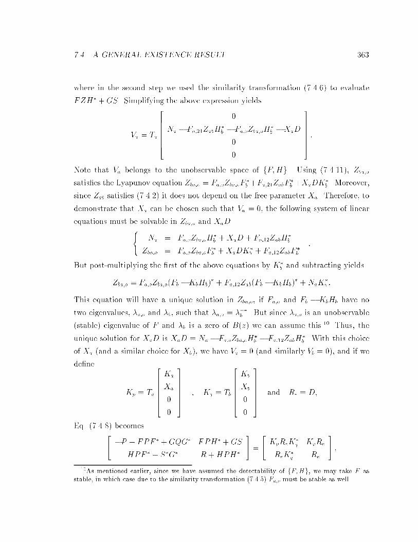
���� A GENERAL EXISTENCE RESULT �
where in the second step we used the similarity transformation � ���� to evaluate
FZH� �GS� Simplifying the above expression yields
Va � Ta
��������
�
Na � Fa���ZabH�
b � Fa�oZba�oH�
b �XaD
�
�
�� �
Note that Va belongs to the unobservable space of fF�Hg� Using � ������ Zba�o
satis�es the Lyapunov equation Zba�o � Fa�oZba�oF�
b �Fa���ZabF�
b �XaDK�
b � Moreover�
since Zab satis�es � ���� it does not depend on the free parameter Xa� Therefore� to
demonstrate that Xa can be chosen such that Va � �� the following system of linear
equations must be solvable in Zba�o and XaD��� Na � Fa�oZba�oH
�
b �XaD � Fa���ZabH�
b
Zba�o � Fa�oZba�oF�
b �XaDK�
b � Fa���ZabF�
b
�
But post�multiplying the �rst of the above equations by K�
b and subtracting yields
Zba�o � Fa�oZba�o�Fb �KbHb�� � Fa���Zab�Fb �KbHb�
� �NaK�
b �
This equation will have a unique solution in Zba�o� if Fa�o and Fb � KbHb have no
two eigenvalues� �a�o and �b� such that �a�o � ���b � But since �a�o is an unobservable
�stable� eigenvalue of F and �b is a zero of B�z� we can assume this��� Thus� the
unique solution for XaD is XaD � Na � Fa�oZba�oH�
b � Fa���ZabH�
b � With this choice
of Xa �and a similar choice for Xb�� we have Va � � �and similarly Vb � ��� and if we
de�ne
Kp � Ta
��������
Ka
Xa
�
�
�� � Kq � Tb
��������
Kb
Xb
�
�
�� and Re � D�
Eq� � ���� becomes�� �P � FPF ��GQG� FPH� �GS
HPF � � S�G� R �HPH�
�� �
�� KpReK
�
q KpRe
ReK�
q Re
�� �
�As mentioned earlier� since we have assumed the detectability of fF�Hg� we may take F asstable� in which case due to the similarity transformation ������� Fa�o must be stable as well�

� CHAPTER �� INFINITE HORIZON RESULTS
which means the SDARE � ���� has a solution� This concludes the proof of part �a��
The proofs of the remaining parts of the Theorem are much shorter� To prove
part �b� if we assume that P is semistabilizing then� since the zeros ofM�z� and N�z�
are the eigenvalues of F �KpH and F �KqH� it is straightforward to see that M�z�
and N�z� are semistable� Therefore the main e�ort is to show the other direction�
Thus� let us assume that a proper semi�canonical �semistabilizing� factorization of
��z� exists� Now note that
T��a �F �KpH�Ta �
��������
Fa � Fa��� �
Fa��� Fa�o Fa��� Fa���
� � Fa�c �
� � Fa��� Fa�co
���
��������
Ka
Xa
�
�
��hHa � Ha�c �
i
��������
Fa �KaHa � Fa����KaHa�c �
Fa����XaHa Fa�o Fa��� �XaHa�c Fa���
� � Fa�c �
� � Fa��� Fa�co
��
Thus the eigenvalues of F �KpH are the union of the eigenvalues of the matrices
�� Fa �KaHa �
Fa����XaHa Fa�o
�� and
�� Fa�c �
� Fa�co
�� �
or� similarly� the matrices
Fa �KaHa � Fa�o � Fa�c and Fa�co�
Since the �rst of the above matrices is semi�stable �by the assumption that a semi�
stable factorization exists� and the remaining three are stable� we conclude that
F � KpH is semi�stable� A similar reasoning shows that F � KqH is semi�stable�
thus ending our proof of part �b��
We now continue with the proof of part �c�� First� suppose that the SDARE has
a Hermitian solution� P � P �� Then we can write the Popov function as
��z� �hH�zI � F ���Kp � I
iRe
hH�z��I � F ���Kp � I
i�
� � �����
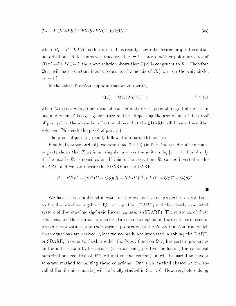
���� A GENERAL EXISTENCE RESULT ��
where Re � R�HPH� is Hermitian� This readily shows the desired proper Hermitian
factorization� �Note� moreover� that for all jzj � � that are neither poles nor zeros of
H�zI�F ���Kp�I� the above relation shows that ��z� is congruent to Re� Therefore
��z� will have constant inertia �equal to the inertia of Re� a�e� on the unit circle�
jzj � ���
In the other direction� suppose that we can write�
��z� �M�z�JM��z���� � ����
whereM�z� is a p�q proper rational transfer matrix with poles of magnitude less than
one and where J is a q � q signature matrix� Repeating the arguments of the proof
of part �a� to the above factorization shows that the SDARE will have a Hermitian
solution� This ends the proof of part �c��
The proof of part �d� readily follows from parts �b� and �c��
Finally� to prove part �d�� we note that � ����� �in fact� its non�Hermitian coun�
terpart� shows that ��z� is nonsingular a�e� on the unit circle� jzj � �� if� and only
if� the matrix Re is nonsingular� If this is the case� then Re can be inverted in the
SDARE� and we can rewrite the SDARE as the DARE
P � FPF � � �FPH� �GS��R �HPH�����FPH� �GS�� �GQG��
We have thus established a result on the existence� and properties of� solutions
to the discrete�time algebraic Riccati equation �DARE� and the closely associated
system of discrete�time algebraic Riccati equations �SDARE�� The existence of these
solutions� and their various properties� turns out to depend on the existence of certain
proper factorizations� and their various properties� of the Popov function from which
these equations are derived� Since we normally are interested in solving the DARE�
or SDARE� in order to check whether the Popov function ��z� has certain properties
and admits certain factorizations �such as being positive� or having the canonical
factorizations required of H� estimation and control�� it will be useful to have a
separate method for solving these equations� One such method �based on the so�
called Hamiltonian matrix� will be brie y studied in Sec� ��� However� before doing

�� CHAPTER �� INFINITE HORIZON RESULTS
so� it will be useful to study the consequence of our results for some special cases of
interest�
��� Special Cases
In this section we shall brie y review some special cases of the general DARE and
SDARE that have been studied so far� These special cases are motivated by appli�
cations in linear quadratic control� linear least�squares �Wiener� �ltering� and H�
control and �ltering �see Secs� �� and ��� and Secs� �� and �� ��
����� The Case of R � � and Q � SR��S� � �
We �rst remark that the case we are considering corresponds to the case where�� Q S
S� R
�� ��
We should also note that there is no loss of generality in considering Q�SR��S� �
instead of Q� SR��S� � �� since we can always go from the latter condition to the
former one by a simple rede�nition of the matrix G�
The so�called �positive� case for the DARE� that we are considering here� arises
in linear quadratic control and linear least�squares �ltering �see e�g�� Theorems ����
and ����� and is very well studied� Therefore� the results given below are well known
�see e�g�� �AM �� Kuc � and the references therein�� However� for completeness� we
will provide brief proofs using the approach presented so far�
Theorem �� �� �The Positive DARE� Consider the DARE
P � FPF � �GQG� � �FPH� �GS��R �HPH�����FPH� �GS��� � �����
where fF�Hg is detectable and
�� Q S
S� R
�� �� Then we have the following results�
�a The DARE always has a Hermitian semi�stabilizing solution such that the ma�
trix F �KpH� with Kp � �FPH��GS��R�HPH���� is semi�stable� i�e�� has
all its eigenvalues inside the closed unit disk�
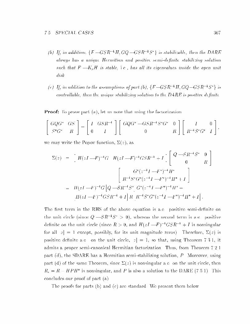
���� SPECIAL CASES �
�b If� in addition� fF �GSR��H�GQ�GSR��S�g is stabilizable� then the DARE
always has a unique Hermitian and positive semi�de�nite stabilizing solution
such that F � KpH is stable� i�e�� has all its eigenvalues inside the open unit
disk�
�c If� in addition to the assumptions of part �b� fF�GSR��H�GQ�GSR��S�g iscontrollable� then the unique stabilizing solution to the DARE is positive de�nite�
Proof� To prove part �a�� let us note that using the factorization
�� GQG� GS
S�G� R
�� �
�� I GSR��
� I
���� GQG� �GSR��S�G� �
� R
���� I �
R��S�G� I
�� �
we may write the Popov function� ��z�� as
��z� �hH�zI � F ���G H�zI � F ���GSR�� � I
i �� Q� SR��S� �
� R
��
�� G��z��I � F ����H�
R��S�G��z��I � F ����H� � I
��
� H�zI � F ���GhQ� SR��S�
iG��z��I � F ����H� �h
H�zI � F ���GSR�� � IiRhR��S�G��z��I � F ����H� � I
i�
The �rst term in the RHS of the above equation is a�e� positive semi�de�nite on
the unit circle �since Q � SR��S� ��� whereas the second term is a�e� positive
de�nite on the unit circle �since R �� and H�zI � F ���GSR�� � I is nonsingular
for all jzj � � except� possibly� for its unit magnitude zeros�� Therefore� ��z� is
positive de�nite a�e� on the unit circle� jzj � �� so that� using Theorem ���� it
admits a proper semi�canonical Hermitian factorization� Thus� from Theorem ����
part �d�� the SDARE has a Hermitian semi�stabilizing solution� P � Moreover� using
part �d� of the same Theorem� since ��z� is nonsingular a�e� on the unit circle� then
Re � R �HPH� is nonsingular� and P is also a solution to the DARE � ������ This
concludes our proof of part �a��
The proofs for parts �b� and �c� are standard� We present them below�

�� CHAPTER �� INFINITE HORIZON RESULTS
For part �b� suppose that P is the Hermitian semi�stabilizing solution to the
DARE� and that x is any left eigenvector of F �KpH with eigenvalue j�j � �� i�e��
x�F �KpH� � �x�
Moreover� note that the DARE can be rewritten as
P � �F �KpH�P �F �KpH�� �hG �Kp
i �� Q S
S� R
���� G�
�K�
p
�� �
Pre and post�multiplying the above expression by x and x�� respectively� we obtain
xPx� � j�j�xPx� � xhG �Kp
i�� Q S
S� R
���� G�
�K�
p
��x��
from which we infer
xhG �Kp
i �� Q S
S� R
���� G�
�K�
p
��x� � ��
But this implies
x�G�Q� SR��S��G� � �GSR�� �Kp�R�GSR�� �Kp�
��x� � ��
from which we infer
xG�Q� SR��S��G�x� � � and xKp � xGSR��� � �����
We now see that
�x � x�F �KpH� � xF � xKpH � xF � xGSR��H � x�F �GSR��H��
i�e� � x is also a left eigenvector of F �GSR��H with eigenvalue �� The �rst equality
in � ����� along with the above result can be rewritten as
xG�Q� SR��S�� � � and x�F �GSR��H� � �x�
This of course contradicts the stabilizability condition� We thus have
j�j ��
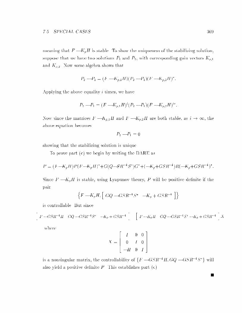
���� SPECIAL CASES ��
meaning that F �KpH is stable� To show the uniqueness of the stabilizing solution�
suppose that we have two solutions P� and P�� with corresponding gain vectors Kp��
and Kp��� Now some algebra shows that
P� � P� � �F �Kp��H��P� � P���F �Kp��H���
Applying the above equality i times� we have
P� � P� � �F �Kp��H�i�P� � P���F �Kp��H�i��
Now since the matrices F �Kp��H and F � Kp��H are both stable� as i � � the
above equation becomes
P� � P� � �
showing that the stabilizing solution is unique�
To prove part �c� we begin by writing the DARE as
P � �F�KpH�P �F�KpH���G�Q�SR��S��G����Kp�GSR���R��Kp�GSR
�����
Since F � KpH is stable� using Lyapunov theory� P will be positive de�nite if the
pair nF �KpH�
hGQ�GSR��S� �Kp �GSR��
iois controllable� But sinceh
F � GSR��H GQ�GSR��S� �Kp � GSR��i�hF �KpH GQ� GSR��S� �Kp � GSR��
iX
where
X �
�����
I � �
� I �
�H � I
��
is a nonsingular matrix� the controllability of fF � GSR��H�GQ � GSR��S�g willalso yield a positive de�nite P � This establishes part �c��

� CHAPTER �� INFINITE HORIZON RESULTS
����� The Case of Nonsingular F � GSR��H
In the previous section we saw that when R � and Q � SR��S� � then each
solution to the SDARE was a solution of the DARE as well� Finding conditions under
which Re is nonsingular� so that solutions of the SDARE are solutions of the DARE
as well� is� in the general case� quite di�cult �see Ex� �� However� it is possible to
give a simple su�cient condition for this to be so�
Theorem �� � �Nonsingular F �GSR��H� Suppose that fF�Hg is detectable andthat R and F �GSR��H are nonsingular� Then any solution to the SDARE ��� ��
is also a solution to the DARE
P � FPF � �GQG� � �FPH� �GS��R �HPH�����FPH� �GS���
Proof� Let P be the solution to the SDARE���������
P � FPF � �GQG� �KpReK�
q
KpRe � FPH� �GS � KqR�
e � FP �H� �GS
Re � R�HPH�
�
Suppose now that Re is singular� Then there exists an x such that
Rex � ��
Therefore if we post�multiply the second set of equations in the SDARE by x we
obtain
�FPH� �GS�x � ��
But
FPH��GS � �F�GSR��H�PH��GSR��HPH��GS � �F�GSR��H�PH��GSR��Re�
so that
�F �GSR��H�PH�x � ��

���� SPECIAL CASES �
But since F � GSR��H is nonsingular� this implies PH�x� We can also conclude
that HPH�x � �� so that
HPH�x � �Re �R�x � �Rx � ��
which is a contradiction since R is assumed invertible� Therefore Re must be nonsin�
gular� and P is a solution to the DARE�
����� The Case of Positive Q� SR��S�
Here we assume that S � �� so that the DARE becomes
P � FPF ��GQG� � FPH��R �HPH����HPF �� � ����
There is� of course� no loss of generality in making this assumption since the general
DARE
P � FPF � �GQG� � �FPH� �GS��R �HPH�����FPH� �GS��
can always be transformed to one with S � �� by rewriting it as
P � �F �GSR��H�P �F �GSR��H�� �G�Q � SR��S��G� ��F �GSR��H�PH��R �HPH����HP �F �GSR��H���
and rede�ning the matrices as
F � F �GSR��H and Q� Q� SR��S��
We therefore will be studying � ���� in the case where Q �� Moreover� we can
always assume that the �possibly� inde�nite matrix R has the form
R �
�� Ip� �
� �Ip�
�� � � ����
The reason being that the DARE can be rewritten as
P � F �I � PH�R��H���PF � �GQG��

� CHAPTER �� INFINITE HORIZON RESULTS
so that what really enters the DARE is the matrix H�R��H and a simple rede�nition
of H will allow R to have the form described in � ����� We shall also partition H
according to the partitioning of R and write
H �
�� H�
H�
�� �
We should also remark that the DARE with Q � and R inde�nite arises in H�
�ltering and control where it plays a prominent role �GD��� DGKF��� KN��� GL����
�See also Theorems ���� and �� ��� The following result on the DARE is known in
the H� literature� but is rarely stated in the form given below�
Theorem �� �� �Positive Q� Consider the DARE
P � FPF ��GQG� � FPH��R �HPH����HPF ��
where
R �
�� Ip� �
� �Ip�
�� � H �
�� H�
H�
�� �
fF�H�g is detectable� fF�GQ���g is stabilizable and Q �� Suppose� moreover� that
the DARE has a Hermitian stabilizing solution� P � Then we have the following results�
�a P � ��
�b If� in addition� R and Re � R �HPH� have the same inertia� then
�i F �K�H is stable� where
K� � FPH�
��Ip� �H�PH�
� ����
�ii The transfer matrix
M�z� �hM��z� M��z�
i�
where
M��z� � H��I � PH�
�H�����zI � F �K�H��
��GQ���

���� SPECIAL CASES
and
M��z� � H�PH�
� �Ip��H�PH�
� ����H��I�PH
�
�H�����zI�F�K�H��
��K�
is strictly contractive on the unit circle� i�e��
M�z�M��z��� Ip�� jzj � ��
Remarks�
�a� Theorem ��� can be used to check whether the Popov function
��z� �hH�zI � F ��� I
i�� GQG� GS
S�G� R
���� �z��I � F ����H�
I
�� �
admits the factorization required for the existence of suboptimal H� �lters�
From Theorem ����� the condition for the existence of an H� �lter of level
� � � is that the Popov function admit the following canonical factorization�
��z� �
�� L���z� L���z�
L���z� L���z�
���� Ip� �
� �Ip�
���� L����z
��� L����z���
L����z��� L����z
���
�� � � �����
with
�� L���z� L���z�
L���z� L���z�
�� and L���z� minimumphase and proper� and L���z� sta�
ble and strictly proper� Now the existence of a canonical Hermitian factorization
is equivalent to the existence of a Hermitian stabilizing solution to the DARE�
That the factorization has the appropriate inertia is equivalent to R and Re
having the same inertia� and the strictly proper property of L���z� and inverse
stability of L���z� can be checked by performing the block LDU decomposition of
Re and checking whether F�K�H is stable� whereK� � FPH�
� �Ip��H�PH�
� ����
Thus we have the following result�
�An H� �lter of level � � � exists if� and only if� there exists a Hermitian
stabilizing solution to the DARE such that the matrices R � Ip� � ��Ip�� andRe � R�HPH� have the same inertia�� But this is precisely the what is stated
in the second part of Theorem �����

CHAPTER �� INFINITE HORIZON RESULTS
�b� The transfer matrixM�z� of Theorem ��� can be seen to be equal to TKcen�z��
the transfer operator that maps the disturbances to estimation errors in the
H� �ltering problem of level � � �� when the central �lter is used� Statement
�b�� part �ii�� of Theorem ��� states the �obvious� fact that when a solution
to the H� �ltering problem exists TKcen�z� is strictly contractive�
Proof of Theorem �� ��� Let us �rst prove part �a� by establishing P � �� To this
end� consider� P� � the stabilizing solution to the DARE��
P� � FP�F� �GQG� � FP�H
��R� �HP�H����HP�F
�� � �����
where
R� �
�� Ip� �
� ��Ip�
�� � � � ��
This DARE may be written as
P� � F �I � P�H�
�H� � ���P�H�
�H����P�F
� �GQG�� � ��� �
We can use the above expression to di�erentiate P� with respect to � and obtain
!P� � dP��d�� Using the identity�
dA��
d�� �A��dA
d�A���
and after some algebra� we may write
!P� � F �I�P�H�
�H�����P�H�
�H�����P�����P�H
�
�H�P���I�P�H�
�H�����P�H�
�H����F ��
� �����
But note that since P� is stabilizing� the matrix
F �I � P�H�
�H� � ���P�H�
�H���� � F �I � P�H
�R��� H���� � F �Kp��H�
is stable� Thus � ����� becomes
!P� � �F �Kp��H�P��F �Kp��H�� � ����F �Kp��H�P�H�
�H�P��F �Kp��H���
��The given DARE is simply the DARE corresponding to the H� �ltering problem with level� � �� Since we have assumed that the level � � � H� �ltering problem has a solution� the samewill be true for all � � �� Therefore� for � � � the given DARE will have a Hermitian stabilizingsolution� as stated�

���� SPECIAL CASES �
Since the second term in the above equation is negative semi�de�nite and since F �KpH is stable� using Lyapunov theory� we have
!P� � ��
Therefore� for all � such that P� is stabilizing� the P� form a nonincreasing function
of Hermitian matrices� In other words� if P�� and P�� are two stabilizing solutions to
the DARE � ������ then
�� � �� implies P�� � P�� �
Now if we let � �� then � ��� � becomes
P� � F �I�P�H�
�H����P�F
��GQG� � FP�F��GQG��FP�H�
� �Ip��H�P�H�
� ���H�P�F
��
But since Q �� this is an example of the positive DARE studied in Sec� �����
Therefore� since fF�H�g is detectable and fF�GQ���g is stabilizable� using Theorem ���� part �b�� a stabilizing solution to this DARE exists and is such that P� � �� Now
from the hypothesis of the Theorem we know that the DARE � ����� has a stabilizing
solution for � � �� As � � � � using the �above established� monotonicity
property of the stabilizing solutions to � ������ we have
P � P� � P� � ��
which proves part �a��
To proceed with the proof of part �b�� we now assume that the matrices
Re � R �HPH� �
�� Ip� �H�PH
�
� H�PH�
�
H�PH�
� �Ip� �H�PH�
�
�� and R �
�� Ip� �
� �Ip�
�� �
have the same inertia� Since P � �� we have Ip� � H�PH�
� �� and therefore the
above inertia condition implies that the Schur complement of the ��� �� block entry
of Re must be negative de�nite� i�e��
�Ip��H�PH�
��H�PH�
� �Ip��H�PH�
� ���H�PH
�
� � �Ip��H��I�PH�
�H����PH�
� ��

� CHAPTER �� INFINITE HORIZON RESULTS
Now we can write the DARE as
P � F �I � PH��H� � PH
��H��
��PF � �GQG�
� F �I � PH��H����PF � �GQG�
�F �I � PH��H����PH��
�H��I � PH��H��
��PH�� � Ip����
H��I � PH��H��
��PF �
� F �I � PH��H��
��PF � �GQG�
�F �I � PH��H��
��PH��
�Ip� �H��I � PH
��H��
��PH��
���� �z �M�
H�P �I �H��H�P �
��F �
� �F �K�H�P �F �K�H�� �GQG� �K�K��� F �I � PH��H��
��PH��MH�P �I �H��H�P �
��F �� �z � �Q�
�
where in the second step we have expanded �I � PH�
�H� � PH�
�H���� using the
matrix inversion lemma� and where in the fourth step we have used the expression
K� � FPH�
� �Ip� � H�PH�
� ���� Now since P � �� fF�G���g is stabilizable� and
GQG� �K�K�
� � "Q �� we can use an argument similar to the argument of Theorem
���� part �b� to show that F�K�H is stable� This proves part �b�i� of this Theorem�
To prove part �b�ii� we proceed as follows� First� note that using the stabilizing
solution to the DARE we can factorize the Popov function as
��z� �
�� L���z� L���z�
L���z� L���z�
���� Re��Ip� �
� �Re��Ip�
���� L���z��� L���z���
L���z��� L���z���
��� � � �����
where both Re�� and Re�� are positive de�nite� �Such a factorization is called a J �
spectral factorization�� Indeed� this factorization is achieved via
��z� �
����� H�
H�
�� �zI � F ���Kp �
�� Ip� �
� Ip�
������� Ip� �H�PH
�
� H�PH�
�
H�PH�
� �Ip� �H�PH�
�
�� fg� �
and the block triangular factorization of the central matrix�� Ip� �H�PH
�
� H�PH�
�
H�PH�
� �Ip� �H�PH�
�
�� ��
� Ip� �
H�PH�
��Ip� �H�PH�
� ��� Ip�
���� Ip� �H�PH
�
� �
� �Re��
���� Ip� �Ip� �H�PH
�
� ���H�PH
�
�
� Ip�
�� �
where Re�� � Ip� �H��I � PH�
�H����PH�
� �� Thus it is readily seen that�� L���z� L���z�
L���z� L���z�
�� �
����� H�
H�
�� �zI � F ���Kp �
�� Ip� �
� Ip�
������� Ip� �
H�PH�
��Ip� �H�PH�
� ��� Ip�
�� �

���� SPECIAL CASES
Some algebra now shows that
L���z� � H��zI � F ���K� � Ip�� � ������
and
L���z� � H��zI � F ���K� �H�PH�
� �Ip� �H�PH�
� ���� � ������
We may also remark that since F �K�H is stable� the transfer matrix L���z� has a
stable inverse� Now using the factorization � ����� it is straightforward to see
h�L���z�L���� �z� Ip�
i��z�
�� L���� �z���L����z���
Ip�
�� �
��L���z�� L���z�L���� �z�L���z�
�Re��
�L���z���� L���z���L���� �z
���L���z����� ��
� ������
for all jzj � �� Note that the inequality is strict since L�� � L���z�L���� �z�L���z� has
no unit circles zeros �in turn because
�� L���z� L���z�
L���z� L���z�
�� has no unit circle zeros #
since P is stabilizing # and L���z� has a stable inverse�� On the other hand� if we
de�ne
H��z� � H��zI � F ���GQ��� and H��z� � H��zI � F ���GQ���� � �����
we may write
��z� �
�� Ip� �H��z�H�
��z��� H��z�H�
��z���
H��z�H�
��z��� �Ip� �H��z�H�
��z���
�� �
With the above expression for the Popov function we readily see that
h�L���z�L���� �z� Ip�
i��z�
�� L���� �z���L����z���
Ip�
�� �
�H��z��L���z�L���� �z�H��z�
� �H��z����L���z���L���� �z
���H��z�����
��L���z�L���� �z�
� �L���z���L���� �z
����� � Ip��
Coupling the above equation with the strict inequality of � ������ we obtain�H��z��L���z�L���� �z�H��z�
� �H��z����L���z���L���� �z
���H��z�����
��L���z�L���� �z�
� �L���z
���L���� �z���
��
Ip��

� CHAPTER �� INFINITE HORIZON RESULTS
for all jzj � �� Therefore the transfer matrix
hH��z�� L���z�L���� �z�H��z� L���z�L���� �z�
i�
is strictly contractive on the unit circle� Using the expressions for L���z� and L���z�
�see � ������ ������� and those for H��z� and H��z� �see � ������� it is not too di�cult
to show that
H��z�� L���z�L���� �z�H��z� � H��I � PH�
�H�����zI � F �K�H��
��GQ����
and
L���z�L���� �z� � H�PH�
� �Ip� �H�PH�
� ��� �H��I �PH�
�H�����zI �F �K�H��
��K��
thus proving part �b�ii��
�� The Hamiltonian Matrix
In the previous sections we developed general conditions for the existence of solutions
to the DARE� and the closely related SDARE� in terms of the existence of certain
proper factorizations of the associated Popov function� We then characterized the
properties of these solutions in terms of the properties of the aforementioned factor�
izations� However� in most applications� such as in H� problems� one is interested
in establishing the properties of the Popov function itself� e�g�� whether a canonical
factorization of a certain type exists or not� Therefore it would be very useful �and
indeed essential� to have an independent means of checking whether a solution to the
DARE exists� and if so� of actually computing this solution� If this is possible� then
one can then infer the properties of the Popov function from the properties of the
�computed� Riccati solution�
There now exists a vast �and growing� literature on how to obtain solutions to
algebraic Riccati equations� albeit mostly in the positive case �see the survey paper
�Lau��� and the references therein�� Although it is beyond the scope of this chapter

��� THE HAMILTONIAN MATRIX �
to study �or even mention� all of the various methods for computing solutions to the
DARE� in this section we shall investigate one possible method for computing the
semi�stabilizing solution to the DARE� We shall essentially show that the wellknown
method of invariant subspaces of the Hamiltonian matrix �Pot��� Mac�� Lau ��
extends to the case of DARE�s with inde�nite Q and R�
We also remark that in what follows� without loss of generality� we shall assume
that S � ��
����� The Case of Nonsingular F
We begin by assuming that F is nonsingular� This simpli�es some of the arguments�
More importantly� from Theorem ����� it implies that� whenever a solution to the
SDARE exists� a solution to the DARE also exists� Moreover� it also implies that the
matrix
F �KpH � F � FPH��R�HPH���� � F �I � PH�R��H����
is always invertible� Studying the general case of a �possibly� singular F is more
complicated� We mention what may amount to a promising route for this problem in
the next section�
We continue by attempting to write the DARE as a quadratic form in P � To this
end� we �rst note that the DARE may be rewritten as
�P � F �I � PH�R��H���PF � �GQG� � ��
or� upon premultiplying by �I � PH�R��H�F��� as
�I � PH�R��H�F����P �GQG�� � PF � � ��
Gathering terms yields
hI �P
i �� F�� �F��GQG��H�R��HF�� F � �H�R��HF��GQG�
���� P
I
�� � �� � �����
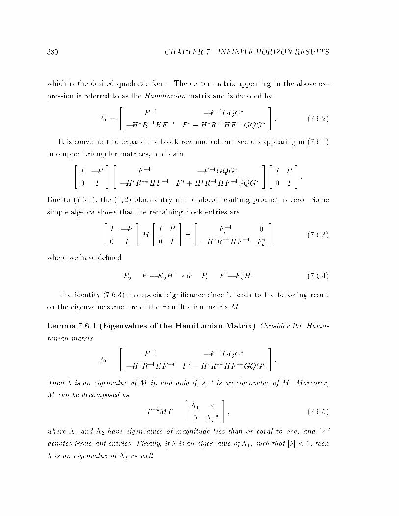
�� CHAPTER �� INFINITE HORIZON RESULTS
which is the desired quadratic form� The center matrix appearing in the above ex�
pression is referred to as the Hamiltonian matrix and is denoted by
M �
�� F�� �F��GQG��H�R��HF�� F � �H�R��HF��GQG�
�� � � �����
It is convenient to expand the block row and column vectors appearing in � �����
into upper triangular matrices� to obtain�� I �P� I
���� F�� �F��GQG��H�R��HF�� F � �H�R��HF��GQG�
���� I P
� I
�� �
Due to � ������ the ��� �� block entry in the above resulting product is zero� Some
simple algebra shows that the remaining block entries are�� I �P� I
��M
�� I P
� I
�� �
�� F��p �
�H�R��HF�� F �q
�� � ����
where we have de�ned
Fp � F �KpH and Fq � F �KqH� � ����
The identity � ���� has special signi�cance since it leads to the following result
on the eigenvalue structure of the Hamiltonian matrixM �
Lemma ����� �Eigenvalues of the Hamiltonian Matrix� Consider the Hamil�
tonian matrix
M �
�� F�� �F��GQG��H�R��HF�� F � �H�R��HF��GQG�
�� �
Then � is an eigenvalue of M if� and only if� ��� is an eigenvalue of M � Moreover�
M can be decomposed as
T��MT �
�� �� �
� ����
�� � � �����
where �� and �� have eigenvalues of magnitude less than or equal to one� and ���denotes irrelevant entries� Finally� if � is an eigenvalue of ��� such that j�j �� then
� is an eigenvalue of �� as well�

��� THE HAMILTONIAN MATRIX ��
Proof� The results are a direct consequence of � ����� Note that since
�� I �P� I
�� �
�� I P
� I
���� �
the HamiltonianM is similar to the block diagonal matrix
�� F��p �
�H�R��HF�� F �q
�� �
Therefore the set of eigenvalues of M is the union of the set of eigenvalues of F��p
and the set of eigenvalues of F �q � Now from the factorization of the Popov function�
��z� �hH�zI � F ���Kp � I
iRe
hH�z��I � F ���Kq � I
i��
we see that the zeros of M�z� are the eigenvalues of Fp and F��q � Therefore� we
conclude that the eigenvalues of M are simply the inverse of the zeros of the Popov
function� ��z�� Since ��z� is para�Hermitian� for every zero at � there exists a zero
at ���� The same is therefore true of the eigenvalues of M � This establishes the �rst
claim of the Lemma�
The decomposition � ����� follows immediately from � ����� We can then readily
identify the �� with the eigenvalues of F �q and �� with the eigenvalues of F �p � which
means that they both have eigenvalues of magnitude less than or equal to one �since
Fp and Fq are semi�stable�� Due to the above factorization of the para�Hermitian
Popov function� ��z�� we see that Fp and Fq have the same eigenvalues of magnitude
strictly less than one� The same is therefore true of �� and ��� thus �nishing the
proof of this Lemma�
The above Lemma furnishes a method for computing solutions to the DARE �when
they exist�� To see why� let us suppose that P is a solution of the DARE and write
� ���� as
M
�� I P
� I
�� �
�� I P
� I
���� F��p �
�H�R��HF�� F �q
�� �

�� CHAPTER �� INFINITE HORIZON RESULTS
from which we may conclude
M
�� P
I
�� �
�� P
I
��F �q � � �����
Now from the proof of Lemma ����� we have identi�ed the eigenvalue structure
of F �q with ��� Therefore there must exist a similarity transformation relating these
two matrices� i�e��
F �q � W��W���
so that we may write � ����� as
M
�� PW
W
�� �
�� PW
W
�����
If we now de�ne T�� � W and T�� � PW � then we may write
M
�� T��
T��
�� �
�� T��
T��
����� � ��� �
Note that in the above expression the matrix T�� is invertible� This means that P �
the solution to the DARE� may be found via
P � T��T���� � � �����
This is an important result since it has allowed us to write the stabilizing solution
of the DARE in terms of elements of the �generalized� eigenvalue decomposition of
M � We formalize this result in the following Theorem�
Theorem ����� �The Invariant Subspace Method� Consider the DARE
P � FPF � �GQG� � FPH��R �HPH����HPF ��
and suppose that F is invertible and fF�Hg is detectable� Then we have the following
results�

��� THE HAMILTONIAN MATRIX �
�a The DARE has a solution if� and only if� there exists a basis�hT ��� T ���
i��
for some n�dimensional invariant subspace of the Hamiltonian matrix� M � such
that T�� is invertible� In other words� if� and only if� there exist T�� and T��
given by
�� F�� �F��GQG��H�R��HF�� F � �H�R��HF��GQG�
���� T��
T��
�� �
�� T��
T��
����� � �����
where �� is an n � n matrix that represents n �of the �n eigenvalues of M �
and T�� is invertible� In this case� the solution of the DARE is given by
P � T��T���� � � ������
�b The DARE has a semistabilizing solution if� and only if� there exists a ba�
sis�hT ��� T ���
i�� for some n�dimensional semistable invariant subspace of the
Hamiltonian matrix� M � such that T�� is invertible� In other words� if� and only
if� there exist T�� and T�� given by ������� where now �� is an n � n matrix
that has all its eigenvalues inside the closed unit disk� and T�� is invertible� In
this case� P is given by ��������
�c The DARE has a stabilizing solution if� and only if� the Hamiltonian matrix�
M � has no unit circle eigenvalues� and�hT ��� T ���
i�� the n�dimensional stable
invariant subspace of M is such that T�� is invertible� In this case� P is given
by ��������
Proof� The proof is quite straightforward� We have already shown that if a solution
to the DARE exists then a basis for some invariant subspace of M with T�� invertible
exists� On the other hand� it is easy to show that if a basis� with the aforementioned
properties� for some invariant subspace of M exists� then T��T���� is a solution to the
DARE�
Finally� the claims of parts �b� and �c� follow from the fact that the eigenvalues
of �� �associated with the eigenvalues of the invariant subspace under consideration�
coincide with the eigenvalues of F �q � Moreover� M can only have a stable invariant
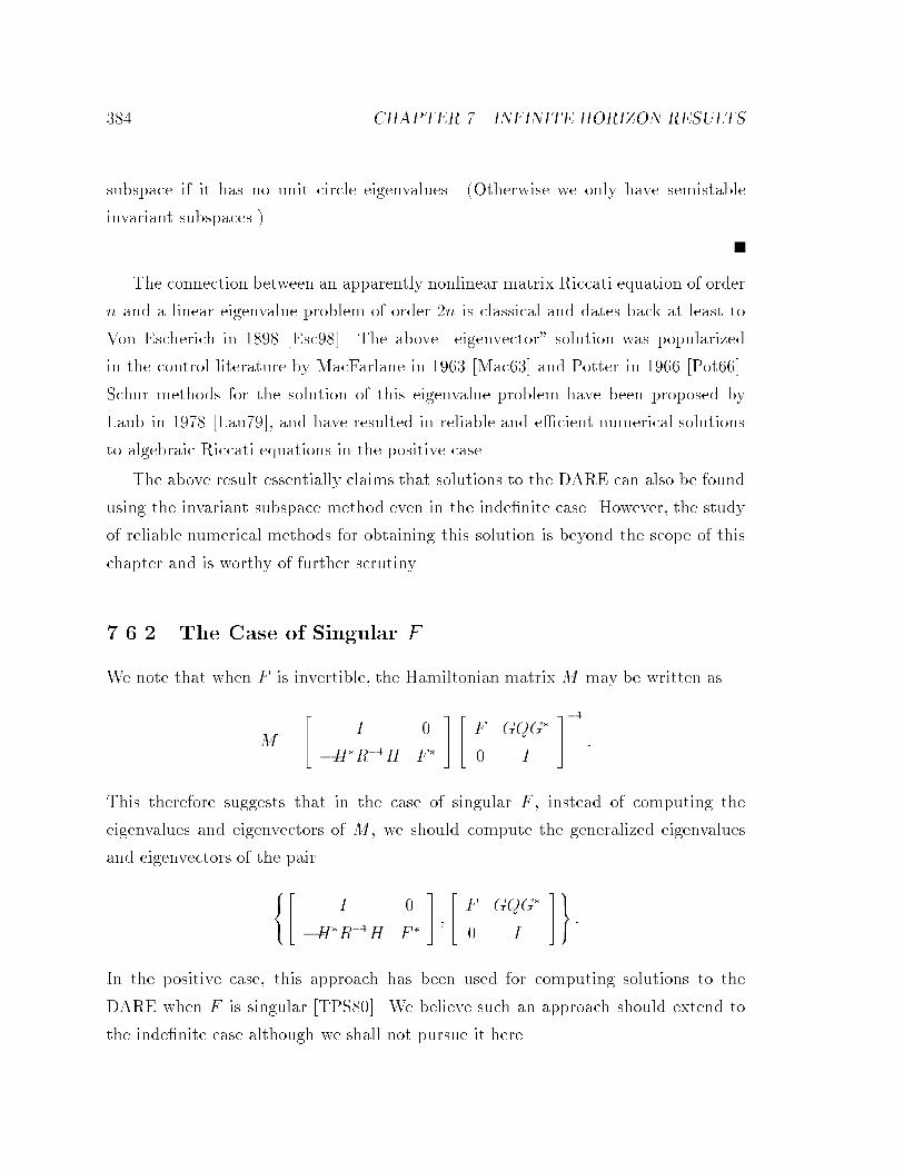
� CHAPTER �� INFINITE HORIZON RESULTS
subspace if it has no unit circle eigenvalues� �Otherwise we only have semistable
invariant subspaces��
The connection between an apparently nonlinear matrix Riccati equation of order
n and a linear eigenvalue problem of order �n is classical and dates back at least to
Von Escherich in ���� �Esc���� The above �eigenvector� solution was popularized
in the control literature by MacFarlane in ��� �Mac�� and Potter in ���� �Pot����
Schur methods for the solution of this eigenvalue problem have been proposed by
Laub in �� � �Lau ��� and have resulted in reliable and e�cient numerical solutions
to algebraic Riccati equations in the positive case�
The above result essentially claims that solutions to the DARE can also be found
using the invariant subspace method even in the inde�nite case� However� the study
of reliable numerical methods for obtaining this solution is beyond the scope of this
chapter and is worthy of further scrutiny�
����� The Case of Singular F
We note that when F is invertible� the Hamiltonian matrix M may be written as
M �
�� I �
�H�R��H F �
���� F GQG�
� I
���� �
This therefore suggests that in the case of singular F � instead of computing the
eigenvalues and eigenvectors of M � we should compute the generalized eigenvalues
and eigenvectors of the pair
����� I �
�H�R��H F �
�� ��� F GQG�
� I
����� �
In the positive case� this approach has been used for computing solutions to the
DARE when F is singular �TPS���� We believe such an approach should extend to
the inde�nite case although we shall not pursue it here�
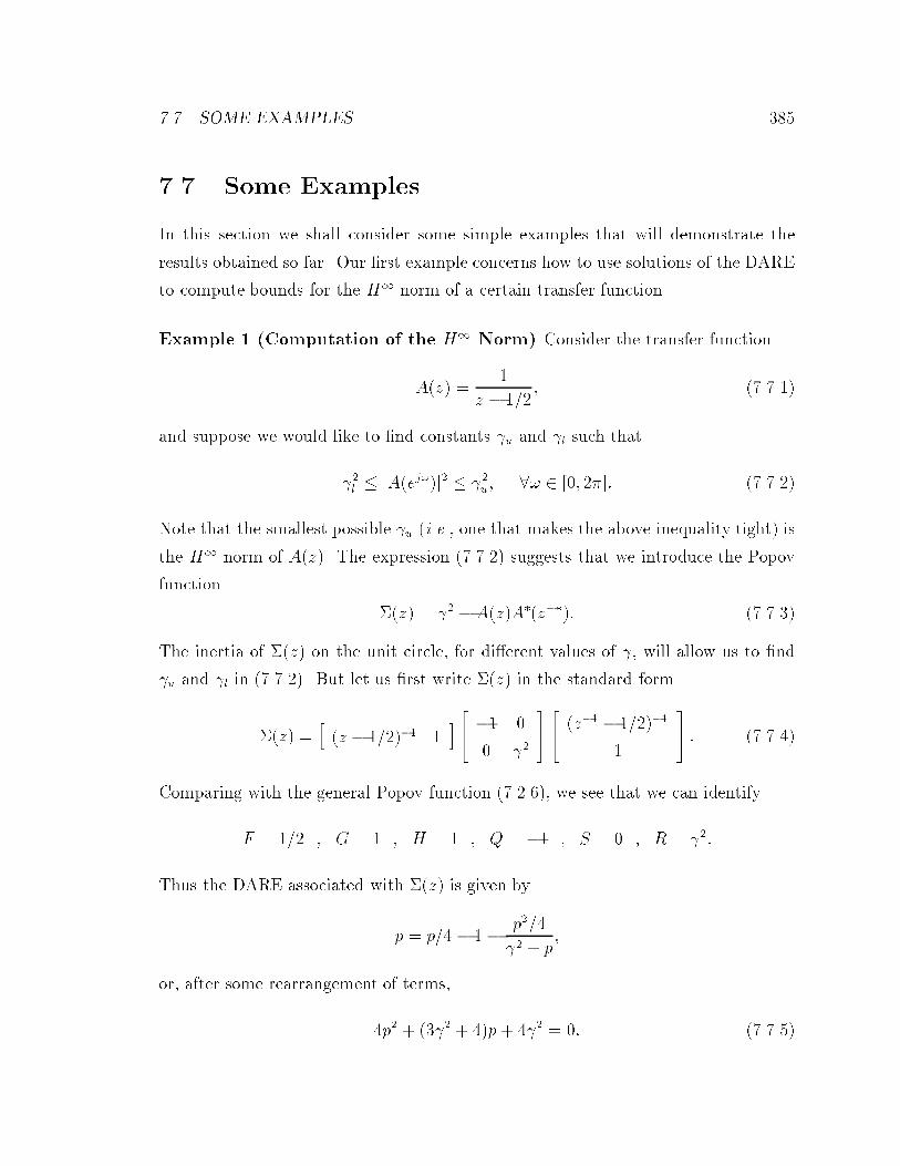
���� SOME EXAMPLES ��
��� Some Examples
In this section we shall consider some simple examples that will demonstrate the
results obtained so far� Our �rst example concerns how to use solutions of the DARE
to compute bounds for the H� norm of a certain transfer function�
Example � �Computation of the H� Norm� Consider the transfer function
A�z� ��
z � ���� � � ���
and suppose we would like to �nd constants �u and �l such that
��l � jA�ej��j� � ��u� � � ��� ���� � � ���
Note that the smallest possible �u �i�e�� one that makes the above inequality tight� is
the H� norm of A�z�� The expression � � ��� suggests that we introduce the Popov
function
��z� � �� �A�z�A��z���� � � ��
The inertia of ��z� on the unit circle� for di�erent values of �� will allow us to �nd
�u and �l in � � ���� But let us �rst write ��z� in the standard form
��z� �h�z � ������ �
i �� �� �
� ��
���� �z�� � ������
�
�� � � � ��
Comparing with the general Popov function � ������ we see that we can identify
F � ��� � G � � � H � � � Q � �� � S � � � R � ���
Thus the DARE associated with ��z� is given by
p � p� � �� p��
�� � p�
or� after some rearrangement of terms�
p� � ��� � �p � �� � �� � � ���

�� CHAPTER �� INFINITE HORIZON RESULTS
Note that� being a quadratic equation in p� the above DARE always has a solution
�see Theorem ����� Now solutions to the DARE are given by
p��� ��
������ � �
q��� � ��� � ��
��
The DARE will therefore have real �corresponding to Hermitian� solutions if� and
only if�
��� � ��� � �� � ��
or equivalently� if� and only if�
�� � or �� �
��
Thus for the above values of �� the Popov function� ��z�� admits Hermitian factor�
izations� and will have constant inertia on the unit circle� By Theorem ���� this
constant inertia is given by the inertia of Re� But
Re��� � �� � p��� ��
������ � �
q���� � �� � ����
��
Therefore for �� � � we have Re �� and for �� � � � we have Re �� Hence ��z�
is non�negative on the unit circle for all �� � � and is non�positive on the unit circle
for all �� � � ��� Thus� we conclude that
��u � sup��������
jA�ej��j� � and ��l � inf��������
jA�ej��j� �
��
which is what we had set out to �nd�
We should also mention that for intermediate values of �� i�e�� � �� �
the DARE does not have a real �Hermitian� solution� and that therefore the Popov
function ��z� does not have constant inertia on the unit circle� jzj � ��
Example �Properties of the DARE� We now continue with the DARE of Ex�
ample � and establish some of its properties� First� we verify that it always has a
semi�stabilizing solution� To this end� note that we may write
Fp � F �KpH � F �I � PH�R��H��� �FR
R �HPH��FR
Re�
��Correspondingly� �z� is positive and negative on the unit circle for all �� � � and �� � �
�
respectively�

���� SOME EXAMPLES �
Therefore
Fp��� �����
���h��� � �
q���� � �� � ����
i � ��
��� � �q���� � �� � ����
�
Now it is straightforward to see that
Fp�Fp� � ��
Therefore at least one of Fp� or Fp� is semi�stable� meaning that at least one of p� or
p� is semi�stabilizing� To be more speci�c� when �� � we have
Fp� ���
�� � ��� � � �q���� � �� � ����
��
so that p� is the stabilizing solution� Likewise� when �� � � we have
Fp� ���
��� � �� �����q���� � �� � ����
���
so that �� Fp� �� and p� is the stabilizing solution� In either case� we have
Kp � Kq �where Kp corresponds to the stabilizing solution�� so that the spectral
factorization of ��z� is given by
��z� �
�Kp
z � ���� �
Re
�Kp
z�� � ���� �
�z � ��� �Kp
z � ���Re
z�� � ��� �Kp
z�� � ����
In the case where � �� � we have
Fp��� ���
��� � � jq���� � ���� � ��
�
Therefore� it is easy to see that
jFp���j � ��
so that both p� and p� are semi�stabilizing solutions� In this case� we have Fp� � F �p��
so that the spectral factorization of ��z� is given by
��z� �z � Fp
z � ���Re
z�� � Fp
z�� � ���� jFpj � ��

�� CHAPTER �� INFINITE HORIZON RESULTS
If we compare this factorization with the factorization ��z� � M�z�N��z���� given
in Lemma ��� we can identify
M�z� �z � Fp
z � ���and N�z� � R�e
z � F �pz � ���
�
Therefore the zero of N�z� is the complex conjugate of the zero of M�z��
Example � �The Hamiltonian Matrix� We once more return to the DARE of
Example �� and now study its associated Hamiltonian matrix
M �
�� � �
����� ��� � ����
�� � � � ���
It is easy to see that the characteristic equation corresponding to M is
�� � ���� � ������ � � � ��
whose solutions are
���� �� � ��� �
q�� � ����� � ��
�
Suppose� for example� that �� � � In this case the stable eigenvalue of M is given
by
�� �� �� � ��� �
q��� ����� � ��
��
A basis for the stable invariant subspace of M can be found by solving the equations
M
�� x
y
�� � ��
�� x
y
�� �
which yields
x � � and y ��� ��� �
q�� � ����� � ��
��
Thus� the stabilizing solution to the DARE is given by
p � xy�� ���� � �
q���� � �� � ����
��

���� SOME EXAMPLES ��
which corresponds to the solution obtained in Example ��
As an example of the case where � � �� � � let us consider � � �� In this case
we have�
���� ��� j
p��
�
and therefore a basis for a semi�stable invariant subspace of M can be found by
solving the equations
M
�� x
y
�� � � � j
p��
�� x
y
�� �
which yields
x � � and y �� � j
p��
��
and from which we infer that a semi�stabilizing solution to the DARE is given by
p � xy�� �� � j
p��
��
Finally� another case of interest is when �� � � since in this case M has repeated
eigenvalues and may not be diagonalizable� With this choice of �� we have
M �
�� � �
��� �
�� and ���� � ��
so that M is obviously non�diagonalizable� Nonetheless� we can still �nd a basis for
the semi�stable invariant subspace of M by solving the equations
M
�� x
y
�� �
�� � �
���
�
���� x
y
�� �
�� x
y
�� �
which yields�
x � � and y � ��
��
The semi�stabilizing solution to the DARE is therefore given by
p � xy�� � ���
which corresponds to the solution that can be obtained from solving � � ��� when
�� � � The spectral factorization of ��z� now becomes
��z� �z � �
z � ���� � � z�� � �
z�� � ����
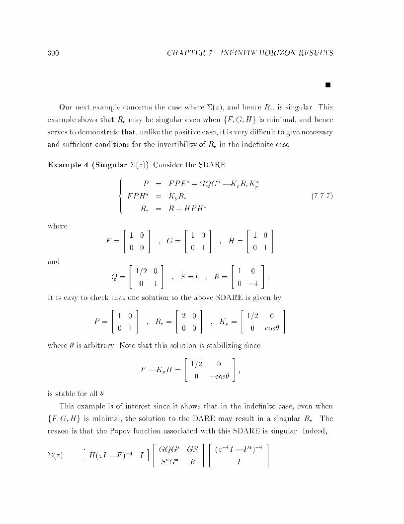
�� CHAPTER �� INFINITE HORIZON RESULTS
Our next example concerns the case where ��z�� and hence Re� is singular� This
example shows that Re may be singular even when fF�G�Hg is minimal� and hence
serves to demonstrate that� unlike the positive case� it is very di�cult to give necessary
and su�cient conditions for the invertibility of Re in the inde�nite case�
Example � �Singular ��z�� Consider the SDARE
���������
P � FPF � �GQG� �KpReK�
p
FPH� � KpRe
Re � R �HPH�
� � � �
where
F �
�� � �
� �
�� � G �
�� � �
� �
�� � H �
�� � �
� �
��
and
Q �
�� ��� �
� �
�� � S � � � R �
�� � �
� ��
�� �
It is easy to check that one solution to the above SDARE is given by
P �
�� � �
� �
�� � Re �
�� � �
� �
�� � Kp �
�� ��� �
� cos
��
where is arbitrary� Note that this solution is stabilizing since
F �KpH �
�� ��� �
� �cos
�� �
is stable for all �
This example is of interest since it shows that in the inde�nite case� even when
fF�G�Hg is minimal� the solution to the DARE may result in a singular Re� The
reason is that the Popov function associated with this SDARE is singular� Indeed�
��z� �hH�zI � F ��� I
i �� GQG� GS
S�G� R
���� �z��I � F ����
I
��

���� SOME EXAMPLES ��
�
���� z � � �
� z
���� I
����������
�� ��� �
� �
�� �
�
�� � �
� ��
��
��
������� z�� � � �
� z��
����
I
��
�
�� �
� � ��z����z����� � � �
� �
�� �
Example �DARE Without SemiStabilizing Solution� Consider the DARE
with F � �� G � �� H �
�� �
�
��� Q � � R �
�� � �
� ��
�� and S �
h� �
i� Using the
fact that the general DARE �with S � �� can be written as
P � F �I � PH�R��H���PF � �GQG��
allows us to write the DARE� in this special case� as
P � P � �
from which we infer P � ��� Thus the DARE has a unique �Hermitian solution�� It
is now straightforward to see that�
Re �
�� � ���� ��
�� � R��e �
�� � ���� �
�� � Kp �
h� ��
i�
from which we can infer�
Fp � F �KpH � F � � � ��
Therefore the solution to the DARE is not �semi�stabilizing� Indeed� although fF�Hgis detectable� and although the DARE has a Hermitian solution� this solution is not
stable� This� of course� means that the Popov function�
��z� �
�� � �
� ��
���
�� �
�
��
�z � ���z�� � ��
h� �
i
�
�� � � �
�z����z������
�z����z�����
��z����z����� �� � �
�z����z�����
��

�� CHAPTER �� INFINITE HORIZON RESULTS
does not admit a proper canonical Hermitian factorization� Using the above solution
to the DARE� the proper factorization that it does admit is given by
��z� �
�� z��
�z����z������
�z����z�����
���z����z�����
z�z����z�����
���� � ���� ��
���� z����
�z����z�������
�z����z�����
��z����z�����
z��
�z����z�����
�� �
which is a �dual� canonical factorization� �Note also that�
�� �
�
��� the stable invariant
subspace of
M �
�� �
� ���
� �
�� �
does not have an invertible T��� whereas the antistable invariant subspace�
�� �
��
��
does��
Example � �DARE Without Solution� Consider the DARE with F � �� G � ��
H �
�� �
�
��� Q � �� R �
�� � �
� ��
�� and S �
h� �
i� Using the fact that the general
DARE �with S � �� can be written as
P � F �I � PH�R��H���PF � �GQG��
allows us to write the DARE� in this special case� as
P � P � ��
from which we infer that the DARE has no solution$ This implies that� despite the
fact that fF�Hg is detectable� the Popov function�
��z� �
�� � �
� ��
���
�� �
�
�� �
�z � ���z�� � ��
h� �
i
�
�� � � �
�z����z������
�z����z�����
��z����z����� �� � �
�z����z�����
��

��� CONCLUSION �
does not admit any proper factorization� �Note that in this case� the only invariant
subspace of the Hamiltonian matrix�
M �
�� � ��� �
�� �
is
�� �
�
�� which does not have an invertible T����
�� Conclusion
In this chapter we studied the discrete�time algebraic Riccati equation �DARE�� and
showed that the existence of solutions to the DARE� or more precisely the system of
discrete�time algebraic Riccati equations �SDARE�� is equivalent to the existence of
a proper factorization of the associated Popov function� Additional properties of the
DARE solution� such as being Hermitian or stabilizing� were then related to additional
properties of the factorization of the Popov function� A method for computing the
solution to the DARE� and� in fact� for checking its existence was also given in terms
of invariant subspaces of the so�called Hamiltonian matrix� We also particularized
these results to some important special cases that are encountered in LQR and H�
estimation and control� Finally� we should mention that the results presented here
are extensions of some wellknown results on discrete�time algebraic Riccati equations
with positive �semi�de�nite coe�cient matrices to the inde�nite �or Krein space�
setting�
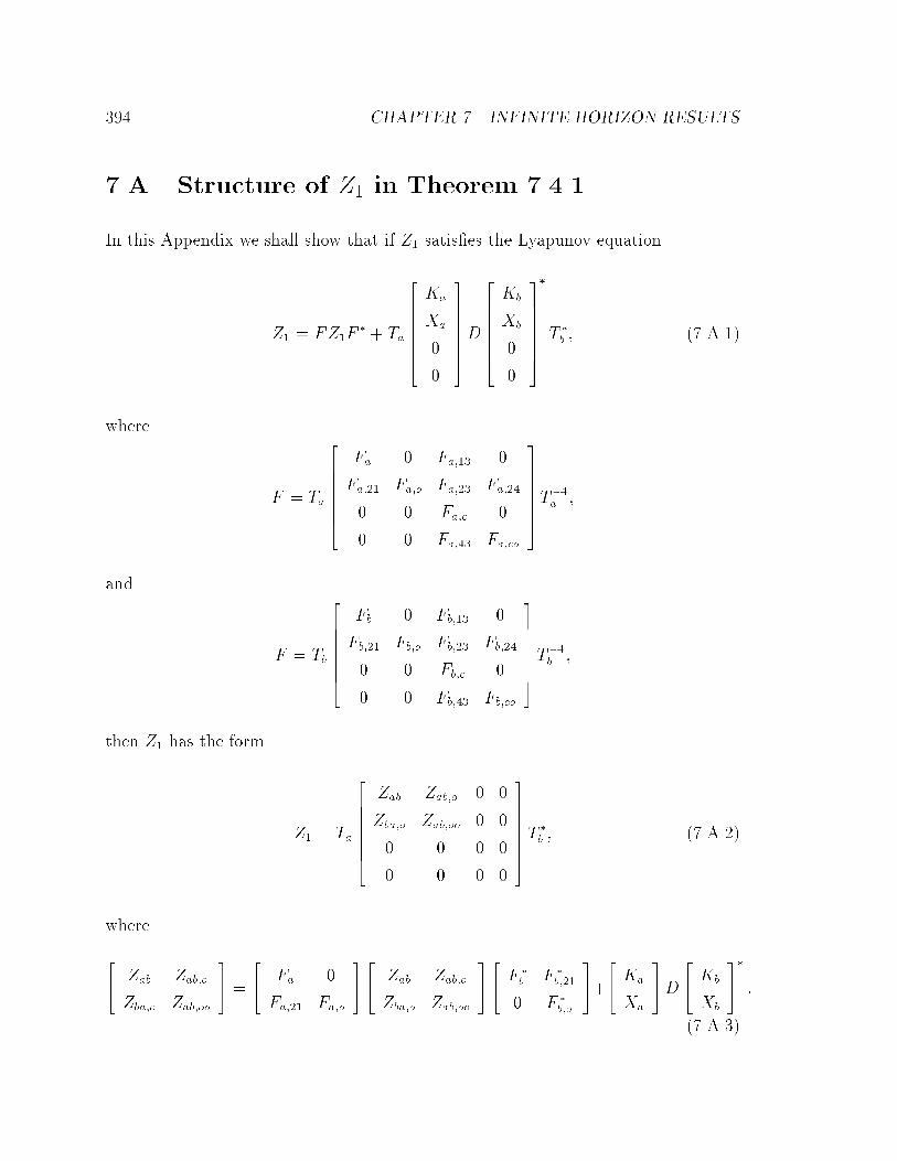
� CHAPTER �� INFINITE HORIZON RESULTS
��A Structure of Z� in Theorem �����
In this Appendix we shall show that if Z� satis�es the Lyapunov equation
Z� � FZ�F� � Ta
��������
Ka
Xa
�
�
��D
��������
Kb
Xb
�
�
��
�
T �b � � �A���
where
F � Ta
��������
Fa � Fa��� �
Fa��� Fa�o Fa��� Fa���
� � Fa�c �
� � Fa��� Fa�co
��T
��a �
and
F � Tb
��������
Fb � Fb��� �
Fb��� Fb�o Fb��� Fb���
� � Fb�c �
� � Fb��� Fb�co
��T
��b �
then Z� has the form
Z� � Ta
��������
Zab Zab�o � �
Zba�o Zab�oo � �
� � � �
� � � �
��T
�
b � � �A���
where
�� Zab Zab�o
Zba�o Zab�oo
�� �
�� Fa �
Fa��� Fa�o
���� Zab Zab�o
Zba�o Zab�oo
���� F �b F �b���
� F �b�o
���
�� Ka
Xa
��D
�� Kb
Xb
��� �
� �A��
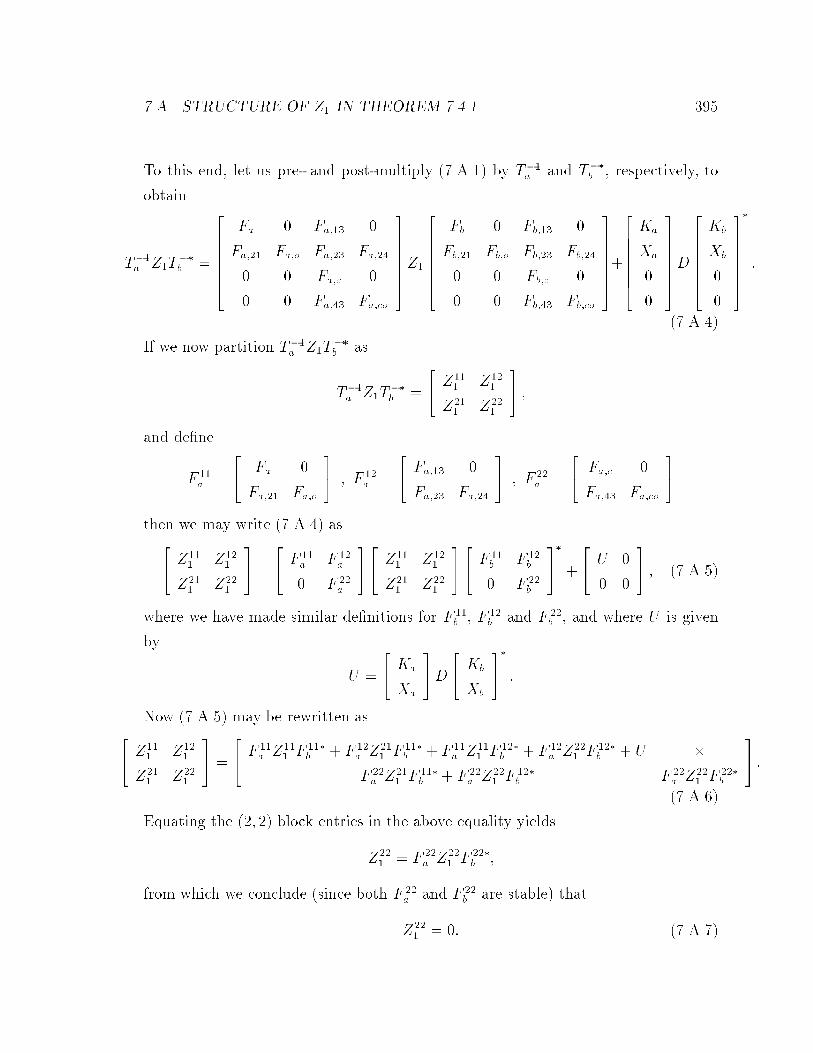
��A� STRUCTURE OF Z� IN THEOREM ����� ��
To this end� let us pre� and post�multiply � �A��� by T��a and T��b � respectively� to
obtain
T��a Z�T��
b �
��������
Fa � Fa��� �
Fa��� Fa�o Fa��� Fa���
� � Fa�c �
� � Fa��� Fa�co
��Z�
��������
Fb � Fb��� �
Fb��� Fb�o Fb��� Fb���
� � Fb�c �
� � Fb��� Fb�co
���
��������
Ka
Xa
�
�
��D
��������
Kb
Xb
�
�
��
�
�
� �A��
If we now partition T��a Z�T��
b as
T��a Z�T��
b �
�� Z��
� Z���
Z��� Z��
�
�� �
and de�ne
F ��a �
�� Fa �
Fa��� Fa�o
�� � F ��
a �
�� Fa��� �
Fa��� Fa���
�� � F ��
a �
�� Fa�c �
Fa��� Fa�co
��
then we may write � �A�� as�� Z��
� Z���
Z��� Z��
�
�� �
�� F ��
a F ��a
� F ��a
���� Z��
� Z���
Z��� Z��
�
���� F ��
b F ��b
� F ��b
��� �
�� U �
� �
�� � � �A���
where we have made similar de�nitions for F ��b � F ��
b and F ��b � and where U is given
by
U �
�� Ka
Xa
��D
�� Kb
Xb
��� �
Now � �A��� may be rewritten as�� Z��
� Z���
Z��� Z��
�
�� �
�� F ��
a Z��� F
���b � F ��
a Z��� F ���
b � F ��a Z��
� F���b � F ��
a Z��� F
���b � U �
F ��a Z��
� F ���b � F ��
a Z��� F
���b F ��
a Z��� F ���
b
�� �
� �A���
Equating the ��� �� block entries in the above equality yields
Z��� � F ��
a Z��� F ���
b �
from which we conclude �since both F ��a and F ��
b are stable� that
Z��� � �� � �A� �

�� CHAPTER �� INFINITE HORIZON RESULTS
Using the above result and equating the ��� �� block entries yields
Z��� � F ��
a Z��� F ���
b �
from which we conclude �since F ��a is stable and F ��
b is marginally stable� that
Z��� � �� � �A���
A similar argument shows that
Z��� � �� � �A���
Eqs� � �A� � �A��� show that Z� has the desired structure given in � �A���� Finally�
� �A�� follows from equating the ��� �� block entries in � �A����

Chapter �
Asymptotic Behaviour
In this chapter we shall focus on the behaviour of the Riccati recursion as time pro�
gresses to in�nity� In order to do so� we shall con�ne our attention to time�invariant
state�space models� Our main interest is to �nd conditions under which� for a given
initial condition� the solution to the Riccati recursion converges to a solution of the
DARE� The main result uses an identity that relates the solution of the Riccati recur�
sion for one initial condition to the solution for another initial condition� and states
that if a certain inertia condition is met� then the Riccati recursion converges to the
unique stabilizing solution �assuming such a solution exists� of the DARE� In the
general case� the aforementioned inertia conditions need to be recursively checked�
however� in some special cases they may be reduced to more simple and more explicit
requirements on the initial condition� In particular� when the coe�cient matrices
of the Riccati recursion are positive semi�de�nite� we can guarantee the convergence
of the Riccati recursion for some inde�nite� and even negative semi�de�nite� initial
conditions �provided they are bounded below by a certain negative semi�de�nite ma�
trix�� Moreover� in the case frequently encountered in H� �ltering and control� we
can guarantee convergence for all positive semi�de�nite initial conditions that are less
than or equal to the unique positive semi�de�nite solution of a related Lyapunov equa�
tion� Finally� we mention some implications of the results obtained here to dierent
problems in which these Riccati equations occur�
��
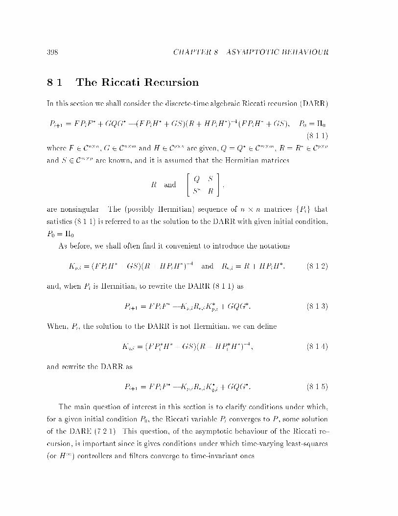
� CHAPTER �� ASYMPTOTIC BEHAVIOUR
��� The Riccati Recursion
In this section we shall consider the discrete�time algebraic Riccati recursion �DARR�
Pi�� � FPiF� �GQG� � �FPiH
� �GS��R �HPiH�����FPiH
� �GS�� P� � ��
� �����
where F � Cn�n� G � Cn�m and H � Cp�n are given� Q � Q� � Cm�m� R � R� � Cp�p
and S � Cm�p are known� and it is assumed that the Hermitian matrices
R and
�� Q S
S� R
�� �
are nonsingular� The �possibly Hermitian� sequence of n � n matrices fPig that
satis�es � ����� is referred to as the solution to the DARR with given initial condition�
P� � ���
As before� we shall often �nd it convenient to introduce the notations
Kp�i � �FPiH� �GS��R � HPiH
���� and Re�i � R �HPiH�� � �����
and� when Pi is Hermitian� to rewrite the DARR � ����� as
Pi�� � FPiF� �Kp�iRe�iK
�p�i �GQG�� � ����
When� Pi� the solution to the DARR is not Hermitian� we can de�ne
Kq�i � �FP �i H� �GS��R �HP �i H
����� � �����
and rewrite the DARR as
Pi�� � FPiF� �Kp�iRe�iK
�q�i �GQG�� � �����
The main question of interest in this section is to clarify conditions under which�
for a given initial condition P�� the Riccati variable Pi converges to P � some solution
of the DARE �������� This question� of the asymptotic behaviour of the Riccati re�
cursion� is important since it gives conditions under which time�varying least�squares
�or H�� controllers and �lters converge to time�invariant ones�

���� OVERVIEW OF RESULTS ��
In this section we shall give what we believe is a very direct approach to establish�
ing the convergence of the Riccati recursion� Moreover� to the best of our knowledge�
the results obtained here are more general than those to have appeared in the lit�
erature and subsume as special cases all of the earlier given results �Wil��b� LK���
Kuc��� Won� a� BRC��� CW ��� Since the section has quite a few results� it will be
useful to begin with a brief overview of what shall be presented�
��� Overview of Results
We begin by proving two important identities relating the solution of the Riccati
recursion for one initial condition to the solution of the Riccati recursion for another
initial condition� The �rst of these is a local identity �see Lemma ���� while the
second is a global identity �see Lemma ����� The result of Lemma ��� is then used
in Sec� �� to compare the solution of the Riccati recursion for an arbitrary initial
condition� P�� with any solution of the corresponding DARE� The ensuing result is
given in Theorem ���� where it is shown that if a certain sequence of matrices �that
depend on P�� are uniformly bounded for all i � �� then the solution to the Riccati
recursion will exponentially converge to the unique stabilizing solution of the DARE
�assuming such a solution exists�� A su�cient condition for convergence turns out to
be the condition that the matrices�
Re�i � R �HPiH��
have constant inertia �equal to the inertia of Re� for all i � �� where Pi is the solution
of the Riccati recursion with initial condition P��
Theorems ���� and ���� prove the convergence of the zero�initial�condition Ric�
cati recursion �corresponding to P� � �� for the positive case and the case where
Q�SR��S� � �� respectively� The proof in both cases follows from showing that the
sequence of matrices�
R�e�i � R�HP �
i H��
where P �i is the zero�initial�condition Riccati solution� has constant inertia for all
i � ��

��� CHAPTER �� ASYMPTOTIC BEHAVIOUR
The fact that we can establish the convergence of fP �i g to P � the unique stabilizing
solution of the DARE� allows us to obtain more simple and more explicit conditions
for convergence than the aforementioned inertia condition on the fRe�ig� Indeed we
can use Lemma ��� to compare fPig� the solution of the Riccati recursion for an
arbitrary initial condition� to fP �i g� the zero initial condition solution� for which we
have already established convergence� The relationship between fPig and fP �i g can be
expressed more concisely in terms of quantities de�ned via the dual Riccati recursion
P ai�� � F �P a
i F � H�R��H � F �P ai G�Q�� �G�P a
i G���G�P ai F� � �����
de�ned in Sec� ����� The exact relationship is given by
Pi�� � P �i�� � ��
p�i� �� ��hI � P�P
a��i��
i�����
�p�i� �� ���� � �����
where P a��i is the zero initial condition solution to the dual Riccati recursion � �����
and ��p�i��� �� is a certain state transition matrix� Since it can be shown that� under
certain stabilizability conditions� the state transition matrix ��p�i��� �� tends to zero
as i��� to show the convergence of Pi to P �i �and hence to P � we need only show
that the matrixhI � P�P
a��i��
i��is uniformly bounded for all i� In the positive case
�where R � � and Q� SR��S� � �� we establish that a su�cient condition for this
is that the initial condition P� be such that
I � �P a����P��Pa���� � �� � ����
where �P a�����P a���� � P a� is the unique positive semi�de�nite solution to the dual
DARE� The above result� whose precise statement is given in Theorem ����� gives�
in the positive case� a very general description of the basin of attraction of the stabi�
lizing solution P to the Riccati recursion� Note that convergence for P� � � follows
immediately from � ����� However� the condition � ���� also allows for some indef�
inite �and even negative semi�de�nite� initial conditions P�� Indeed� under a certain
controllability assumption� it can be shown that P a is invertible so that � ���� can
be replaced by the more revealing condition
P� � ��P a���� � �����

���� SOLUTIONS TO THE RICCATI RECURSION FORDIFFERENT INITIAL CONDITIONS��
Finally� in the case where Q � SR��S� � � it does not seem to be possible to
replace the condition that Re�i should have constant inertia �equal to the inertia of
Re� for all i � �� with a single condition such as � ����� �Nonetheless� the inertia
condition on Re�i is quite intriguing since it is equivalent to the condition required
for the existence of H� �lters and full�information controllers�� However� it is still
possible to give a simple characterization of the basin of attraction of the stabilizing
solution� P � of the DARE in this case as well� Indeed� Theorem ���� shows that if
the initial condition is chosen such that
� � P� � ��
where � is the unique positive semide�nite solution to the Lyapunov equation� � �
F�F � �GQG�� then fPig converges to P �
��� Solutions to the Riccati Recursion for Di�er�
ent Initial Conditions
We �rst give a certain algebraic identity concerning the Riccati recursion � ������
These identities are wellknown �Nis��� MPG � dS ��� and are very useful for obtain�
ing comparison results for solutions to the Riccati recursion�
Lemma ����� �Riccati Solutions for Di�erent Initial Conditions� Suppose P���i
and P���i are two solutions to the discrete�time Riccati recursion with the same fF�G�Hg
and fQ�R� Sg matrices� but with di�erent initial conditions ����� and ����
� � respectively�
Then we have the following identities
P���i�� � P
���i�� � F
���p�i �P
���i � P
���i �F
����p�i � ����
and
P���i�� � P
���i�� � F
���p�i
h�P
���i � P
���i �� �P
���i � P
���i �H��R
���e�i �
��H�P���i � P
���i �
iF����p�i �
� ����
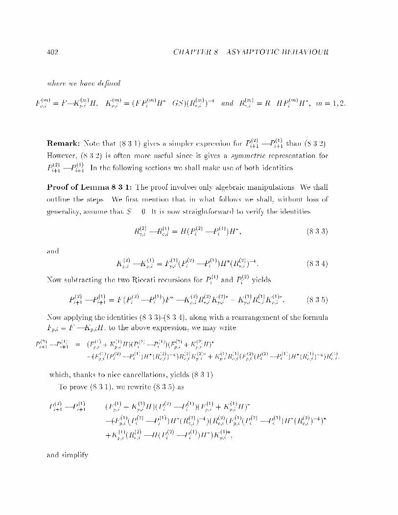
��� CHAPTER �� ASYMPTOTIC BEHAVIOUR
where we have de�ned
F�m�p�i � F�K
�m�p�i H� K
�m�p�i � �FP
�m�i H��GS��R
�m�e�i ��� and R
�m�e�i � R�HP
�m�i H�� m � �� ��
Remark Note that � ���� gives a simpler expression for P ���i�� � P
���i�� than � �����
However� � ���� is often more useful since it gives a symmetric representation for
P���i�� � P
���i��� In the following sections we shall make use of both identities�
Proof of Lemma ����� The proof involves only algebraic manipulations� We shall
outline the steps� We �rst mention that in what follows we shall� without loss of
generality� assume that S � �� It is now straightforward to verify the identities
R���e�i �R
���e�i � H�P ���
i � P���i �H�� � ���
and
K���p�i �K
���p�i � F
���p�i �P
���i � P
���i �H��R
���e�i �
��� � ����
Now subtracting the two Riccati recursions for P���i and P
���i yields
P���i�� � P
���i�� � F �P
���i � P
���i �F � �K
���p�iR
���e�iK
����p�i �K
���p�i R
���e�iK
����p�i � � ����
Now applying the identities � ����� ����� along with a rearrangement of the formula
Fp�i � F �Kp�iH� to the above expression� we may write
P���i�� � P
���i�� � �F
���p�i �K
���p�iH��P
���i � P
���i ��F
���p�i �K
���p�iH��
��F���p�i �P
���i � P
���i �H��R
���e�i �
���R���e�iK
����p�i �K
���p�iR
���e�i �F
���p�i �P
���i � P
���i �H��R
���e�i �
���R���e�i �
which� thanks to nice cancellations� yields � �����
To prove � ����� we rewrite � ���� as
P���i�� � P
���i�� � �F ���
p�i �K���p�iH��P ���
i � P���i ��F ���
p�i �K���p�iH��
��F ���p�i �P ���
i � P���i �H��R���
e�i �����R���
e�i �F���p�i �P ���
i � P���i �H��R���
e�i �����
�K���p�i �R
���e�i �H�P
���i � P
���i �H��K
����p�i �
and simplify�

���� SOLUTIONS TO THE RICCATI RECURSION FORDIFFERENT INITIAL CONDITIONS��
The next identity that we shall establish is just the statement of the fact that
if we know a solution to the Riccati recursion for one initial condition� then under
certain conditions� solutions for other initial conditions can be expressed in terms
of the �rst solution� Although formulas of this type exist in continuous�time �see
�San��� Rei����� we have not encountered their discrete�time analogs in the literature�
We have already provided a local identity relating solutions of the Riccati recursion
for dierent initial conditions in Lemma ���� What we shall now present is a global
identity� The precise statement follows�
Lemma ���� �Riccati Solutions for Di�erent Initial Conditions� Suppose P���i
and P���i are two solutions to the discrete�time Riccati recursion ���� with the same
fF�G�Hg and fQ�R� Sg matrices� but with di�erent initial conditions ����� and ����
� �
respectively� We then have the following identity�
P���i���P
���i�� � ����
p �i��� ��hI � �����
� ������ �O���
i
i�������
� ������ �����
p �i��� ���� � ����
where
����p �i� �� �
���Qi��j�� F
���p�j i � �
I i � �� ����
is the state transition matrix of F���p�j � F �K
���p�jH� and
O���i �
iXj��
����p �j� ���H��R���
e�j ���H����
p �j� ��� � �� �
is the observability Gramian of fF���p�j � �R
���e�j �
����Hg�
Proof We shall prove � ���� by induction� De�ne �Pi�� P
���i �P ���
i � Then for i � ��
using � ����� we have
P���� � P
���� � F
���p��
h�P� � �P�H
��R���e���
��H�P�iF����p��
� ����p ��� ��
hI � �P�H
��R���e���
��Hi�P��
���p ��� ���
� ����p ��� ��
hI � �P�H
��R���e�� �H�P�H
����Hi�P��
���p ��� ���
� ����p ��� ��
hI � �P�H
��R���e���
��Hi��
�P�����p ��� ���
� ����p ��� ��
hI � �P�O
����
i���P��
���p ��� ���

��� CHAPTER �� ASYMPTOTIC BEHAVIOUR
as desired�
Now suppose that � ���� is true for i� We shall show that the identity is true for
i� � as well� Indeed� using � ���� and the above arguments we have
P���i�� � P
���i�� � F
���p�i
h�Pi � �PiH
��R���e�i �
��H�Pi
iF����p�i � F
���p�i
hI � �PiH
��R���e�i �
��Hi��
�PiF����p�i �
�������
On the other hand�
I � �PiH��R
���e�i �
��H � I ����p �i� �
hI � �P�O
���i��
i���P�
���p �i� ��H��R
���e�i �
��H
� I ����p �i� �
hI � �P�O
���i��
i���P�
���p �i� ��H��R
���e�i �
��H���p �i� �� z
O���i�O
���i��
���p �i� ���
� I ����p �i� �
hI � �P�O
���i��
i���P��O
���i �O
���i���
���p �i� ���
� ���p �i� �
hI � �I � �P�O
���i���
���P��O���i � O
���i���
i���p �i� ����
Using the last of the above expressions in � ���� yields
P���i�� � P
���i�� � ���
p �i� �� �hI � �I � �P�O
���i���
���P��O���i �O
���i���
i�����p �i� ����PiF
����p�i
� ���p �i� �� �
hI � �I � �P�O
���i���
���P��O���i �O
���i���
i���I � �P�O
���i���
���P����p �i � �� ��
� ���p �i� �� �
hI � �P�O
���i�� � �P��O
���i � O
���i���
i���P�
���p �i � �� ��
� ���p �i� �� �
hI � �P�O
���i
i���P�
���p �i� �� ���
which is the desired result�
The result of Lemma ��� will prove to be very useful in establishing convergence
results for the Riccati recursion � ������ To see why� suppose is P is some solution to
the DARE �������� Then using � ����� we may write
Pi�� � P � F i��p �I � �P� � P �Op
i ��� �P� � P �F �i����
p � � �����
where Pi is the solution to the Riccati recursion with initial condition P�� and Opi is
the observability Gramian of the pair fFp� R����e Hg� and satis�es the recursion
Opi�� � F �pO
piFp �H�ReH� Op
�� � ��
Now if P is chosen as the stabilizing solution to the DARE �assuming such a solu�
tion exists�� then the matrix Fp � F � KpH is stable and we have limi�� F ip � ��
���� SOME GENERAL CONVERGENCE RESULTS ���
Then using � ������ we see that if the initial condition P� is such that the matrix
�I � �P� � P �Opi ��� �P��P � remains uniformly bounded for all i� then Pi will converge
to P � i�e��
limi��
Pi�� � P � ��
The above line of reasoning will be used in the next section to establish general
convergence results for the Riccati recursion�
��� Some General Convergence Results
In this section we shall obtain some general results concerning the convergence of
the Riccati recursion � ������ We shall essentially give requirements on the initial
condition� P�� such that the solution of the Riccati recursion converges to the unique
stabilizing solution �when a stabilizing solution exists� of the discrete�time algebraic
Riccati equation� Although the requirements on P� may be di�cult to verify in
the general case� in later sections we shall see that� when specialized to some very
important cases of interest in least�squares and H� control and estimation� they result
in easy to verify requirements and yield basins of attraction for the initial condition�
P�� that are more general than those currently available in the literature�
The results presented in this section all use the identity � ������ However� it
will be useful to introduce a more symmetric representation of � ������ To this end�
let us introduce the generalized square�root factorization of the �possibly inde�nite�
Hermitian matrix P� � P � as follows
P� � P � L�JL��� � �����
where J is a signature matrix of appropriate dimensions that represents the inertia
of P� � P � Then using the identity
�I � L�JL��O
pi ���L�JL
�� � L� �J � L��O
piL��
��L���
we may write � ����� as
Pi�� � P � F i��p L� �J � L��O
piL��
��L��F
�i����p � � �����
which is the form that we shall more often use�

��� CHAPTER �� ASYMPTOTIC BEHAVIOUR
Theorem ����� �A General Convergence Result� Consider the discrete�time Ric�
cati recursion
Pi�� � FPiF� �GQG� � �FPiH
� �GS��R �HPiH�����FPiH
� �GS�� � ����
with initial condition� P�� and suppose that the associated DARE ��� � has a stabi�
lizing solution� P � Then if the initial condition P� is chosen such that the matrices
�J � L��OpiL��
���
are uniformly bounded for all i � �� where
P� � P � L�JL���
and Opi satis�es the recursion
Opi�� � F �pO
piFp �H�R��e H� Op
�� � ��
then Pi converges to� P � the unique stabilizing solution of the DARE� Moreover� we
have
kPi � Pk � ��im� � �����
where k � k denotes the spectral radius�
� � kF �KpHk � �� � �����
and
m � supi��
���L� �J � L��OpiL��
��L��
��� � � �����
i�e�� the convergence of Pi to P is exponential�
Two equivalent conditions that ensure the boundedness of �J � L��OpiL��
��are the
following�
�a The matrices J � L��OpiL� have constant inertia �equal to the inertia of J for
all i � ��
�b The matrices Re�i � R � HPiH� have constant inertia �equal to the inertia of
Re for all i � ��

���� SOME GENERAL CONVERGENCE RESULTS ���
Remark The condition given in the above Theorem for convergence to the sta�
bilizing solution of the DARE is essentially that the sequence of matrices T��i �
�J � L��OpiL��
�� be uniformly bounded for all i � �� This condition is interesting
since it only depends on the initial condition through the matrices L� and J �the Opi
do not depend on P��� However� this condition may be quite di�cult to verify in the
general case� The su�cient conditions �a� and �b� for boundedness seem to be much
more restrictive� since instead of requiring that the Ti be uniformly nonsingular for
all i� they require that the Ti have constant inertia for all i� Despite this fact� as we
shall see in subsequent sections� the conditions �a� and �b� are much easier to verify�
and are still quite general since they yield conditions for convergence that are quite
more general than those that have appeared in the literature so far�
Proof of Theorem ����� To prove the �rst part we need only consider � ������
Since P is stabilizing� so that Fp � F �KpH is stable and limi�� F ip � �� and since
�J � L��OpiL��
�� is uniformly bounded for all i � �� we immediately deduce that
limi��
Pi � P � ��
as desired�
To show the exponential convergence of Pi� we can use � ����� to compute kPi�Pk�
Thus� using the submultiplicative property of the spectral radius �kABk � kAk�kBk��
we have
kPi � Pk � kF �KpHki ����L� �J � L��O
piL��
��L��
��� � kF �KpHki�
The desired result � ����� now follows from � ����� and � ������
Now the fact that condition �a� leads to uniformly bounded �J � L��OpiL��
�� for
all i is obvious� since if the J � L��OpiL� have constant inertia �equal to the inertia of
J� for all i� then they are uniformly nonsingular as well� Therefore� what remains to
be shown is that the conditions �a� and �b� are equivalent� This requires somewhat
more eort�
To this end� let us �rst write
Pi � P � LiDiL�i �
�� CHAPTER �� ASYMPTOTIC BEHAVIOUR
where Di is a nonsingular Hermitian matrix of the appropriate dimensions� Now
using � ���� and the above equation� we may write
Pi�� � P � FpLi
hDi �DiL
�iHR
��e�iH
�L�iDi
i��L�iF
�p � � �����
from which we may infer
Li�� � FpLi � F i��p L��
and
Di�� � Di �DiL�iHR
��e�iH
�L�iDi
� Di �DiL�iH�Re�i �HLiDiL
�iH
����H�L�iDi
�hD��
i �H�R��e�iHi��
�
Thus� � ����� may be written as
Pi�� � P � F i��p L�Di��L
��F
�i����p �
Comparing the above expression with � ������ we note that the matrices �J � L��OpiL��
��
will have constant inertia for all i� if� and only if� the matricesDi have constant inertia
for all i�
Now consider the matrix
T �
�� Di DiL
�iH
�
HLiDi Re�i
�� �
Two dierent �block lower�upper and block upper�lower� triangular factorizations of
T show that the matrices�����Di �
� Re�i �HLiDiL�iH
�� z Re�i
� � and
�����Di �DiL
�iHR
��e�iH
�L�iDi� z Di��
�
� Re�i
� � �
are congruent and have the same inertia� Thus Di�� will have the same inertia as Di
if� and only if� Re�i has the same inertia as Re�i� Therefore we conclude that the Di
have constant inertia for all i � � if� and only if� the Re�i have constant inertia �equal
to the inertia of Re� for all i � �� This establishes the equivalence of �a� and �b��

���� CONVERGENCEOFTHE RICCATI RECURSIONWITH ZERO INITIALCONDITION���
�� Convergence of the Riccati Recursion with Zero
Initial Condition
From the discussions of the prior section we conclude that to verify the convergence
of the Riccati recursion for some given initial condition� P�� we need to check the
conditions of Theorem ����� In this section we shall do this for the special case
P� � �� The motivation for doing so is not so much to illustrate an example of
the application of Theorem ����� but rather because understanding the convergence
of the Riccati recursion for P� � � will greatly assist us in obtaining more explicit
convergence results for arbitrary initial conditions� P�� This matter will be taken up
in Sec� ���
����� The Case of R � � and Q � SR��S� � �
Recall from the discussion at the beginning of Sec� ����� that there is no loss of
generality in assuming Q� SR��S� � � as opposed to Q� SR��S� � ��
Now the result given below on the convergence of P �i � the zero�initial�condition
solution to the Riccati recursion� is wellknown �see e�g�� �Wil��b� Kuc��� Won� a�
BRC����� The standard proof of convergence involves showing that the sequence
fP �i g is nondecreasing and� given the detectability condition� bounded from above�
Here� however� we shall give a dierent proof that uses Theorem �����
Theorem ����� �Convergence of Riccati Recursion with P� � �� Consider the
Riccati recursion with zero initial condition
P �i�� � FP �
i F��GQG�� �FP �
i H� �GS��R�HP �
i H�����FP �
i H� �GS��� P �
� � ��
� �����
and suppose that fF�Hg is detectable� fF�GSR��H�GQ�GSR��S�g is stabilizable�
and �� Q S
S� R
�� � ��
��� CHAPTER �� ASYMPTOTIC BEHAVIOUR
Then P �i converges to P � the unique stabilizing and positive semi�de�nite solution of
the discrete�time algebraic Riccati equation
P � FPF � �GQG� � �FPH� �GS��R �HPH�����FPH� �GS���
Proof We �rst remark that� from Theorem ������ since fF�Hg is detectable and
fF �GSR��H�GQ �GSR��S�g is stabilizable� the DARE has a unique stabilizing
and positive semi�de�nite solution� P � Now to prove the Theorem we shall show that
P �i � �� for all i � �� Since R � �� this will imply that
R�e�i � R �HP �
i H� � �� i�
i�e�� that Re�i has constant inertia �equal to the inertia of Re� for all i � �� Therefore
using Theorem ����� the sequence fP �i g must converge to P �
To prove that P �i � �� for all i � �� we proceed by induction� The case i � � is
obvious since P �� � � � �� So let us assume that P �
i � �� for some given i� We then
may write the Riccati recursion as
P �i�� � F �
p�iPiF��p�i �
hG �K�
p�i
i �� Q S
S� R
���� G�
�K��p�i
�� �
Now since Pi � � and
�� Q S
S� R
�� � �� the above expression readily shows that
P �i�� � �� This �nishes our induction and thus proves the Theorem�
����� The Case of Positive Q� SR��S�
As mentioned at the beginning of Sec� ����� there is no loss of generality in assuming
S � � and that the �possibly� inde�nite matrix R has the form
R �
�� Ip� �
� �Ip�
�� �

���� CONVERGENCEOFTHE RICCATI RECURSIONWITH ZERO INITIALCONDITION���
Therefore� in this case our assumption will reduce to Q � �� Moreover� we shall
partition the matrix H according to the partitioning of R and write
H �
�� H�
H�
�� �
In this case� as in the positive case studied in the previous section� our approach
will be to �nd conditions for which the matrices
R�e�i � R�HP �
i H��
have constant inertia for all i � �� where P �i is the zero�initial�condition solution to
the Riccati recursion � ������
Now since R�e�� � R and R�
e�� � Re �assuming we have convergence�� then a
necessary condition for R�e�i to have constant inertia for all i � �� is that R and Re
have the same inertia� The surprising result� given below� is that this is su�cient as
well� More precisely� if a stabilizing solution to the DARE with Q � � exists� then if
R and Re have the same inertia� the R�e�i will have constant inertia for all i�
Theorem ���� �Zero Initial Condition Convergence for Q � �� Consider the
Riccati recursion with zero initial condition
P �i�� � FP �
i F� �GQG� � FP �
i H��R�HP �
i H����HFP �
i F�� P �
� � �� � �����
where
R �
�� Ip� �
� �Ip�
�� � H �
�� H�
H�
�� �
fF�H�g is detectable� fF�GQ���g is stabilizable and Q � �� Suppose� moreover� that
the DARE
P � FPF � �GQG� � FPH��R �HPH����HPF �� � ����
has a stabilizing solution� P � Then if the matrices
R and Re � R �HPH�
have the same inertia� the sequence of matrices fP �i g will converge to P �

��� CHAPTER �� ASYMPTOTIC BEHAVIOUR
Proof The main eort of this proof is to show� under the hypotheses of the Theorem�
that the matrices R�e�i have constant inertia �equal to the inertia of Re� for all i � ��
Once this fact is established� the convergence of P �i to P follows immediately from
Theorem �����
To show that the R�e�i have constant inertia we shall begin with what may appear
as a digression� To this end� consider the time�invariant state�space model��� xi�� � Fxi �GQ���ui
yi � H�xi � vi� �����
and suppose we would like to estimate the linear combination of the states�
si � H�xi� � �����
using the observations fyjgij���� For this purpose� let us construct the estimator
��� �xi�� � F �xi � K��yi �H��xi�
�si � H��xi �H�PH�� �Ip� �H�PH
�� ����yi �H��xi�
� �����
where P is the stabilizing solution to the DARE � ���� and K� � FPH���Ip� �
H�PH�� ���� It is now straightforward to write down a state�space model for the
estimation errors �si � si � �si using � ����� and � ������ as follows��� �xi�� � �F �K�H��xi � GQ���ui �K�vi
�si � H�P �I � PH��H��
���F �K�H��xi �H�PH�� �Ip� �H�PH
�� ���vi
� �����
where we have de�ned �xi � xi � �xi� Taking z�transforms� we may write the above as
�s�z� �hM��z� M��z�
i �� u�z�
v�z�
�� � � ��� �
where
M��z� � H��I � PH��H��
���zI � F �K�H����GQ���
and
M��z� � �H�PH�� �Ip� �H�PH
�� ��� �H��I � PH�
�H�����zI � F �K�H��
��K��
���� CONVERGENCEOFTHE RICCATI RECURSIONWITH ZERO INITIALCONDITION��
But from Theorem ����� since the stabilizing solution to the DARE is such that R
and Re have the same inertia� the transfer matrix M�z� is strictly contractive on the
unit circle� jzj � �� i�e��
M�z�M��z��� � �� jzj � ��
This implies that the mapping from the inputs fuj� vjg�j��� to the estimation error
f�zjg�j��� is strictly contractive� To be more precise� the time�domain representation
of this fact is that
supu�v�l�
k�sk��kuk�� � kvk��
� �� � �����
where the notation k � k� denotes the ��norm of a sequence
kak� ��X
j���
jaij���
and l� is the space of all square�summable sequences�
Let us now �x a constant i � �� and consider the space of those inputs fujg and
fvjg that are zero for all j � i� For this class of inputs we may write � ����� as
P�j��� j�sjj
�Pij��� jujj� �
Pij��� jvjj�
� ��
or P�j��� j�sjj�P��
j��� jujj� �P��
j��� jvjj� �Pi
j�� jujj� �
Pij�� jvjj
�� �� � ������
We now �x a value for x�� the state vector at time zero� and choose the negative part
of the inputs� i�e�� fumj � vmj g
��j���� such that
fumj � vmj g
��j��� � argmin
�� ��Xj���
jujj� �
��Xj���
jvjj�
�� �
where the fuj� vjg satisfy the state�space constraints
xi�� � Fxi �GQ���ui� �� � i � �
and generate the given state vector x�� The solution to the above minimization
problem is wellknown in LQR control �see e�g�� �AM��� KS����� For our purposes�

��� CHAPTER �� ASYMPTOTIC BEHAVIOUR
it su�ces to know that the value of the LQ �linear quadratic� cost function at its
minimum is given by
��Xj���
jumj j� �
��Xj���
jvmj j� � min
fuj �vjg
�� ��Xj���
jujj� �
��Xj���
jvjj�
�� � x���
��x��
where � is the unique positive semide�nite solution to the Lyapunov equation�
� � F�F � �GQG�� � ������
With this particular choice of inputs� we may write � ������ asP�j��� j�sjj�
x�����x� �Pi
j�� jujj� �
Pij�� jvjj
�� ��
or� after discarding the portions of the numerator that involve j � � and j � i�Pij�� j�sjj
�
x�����x� �Pi
j�� jujj� �
Pij�� jvjj
�� �� � ������
Note that in the above inequality the fx�� fujgij��� fvjgij��g are arbitrary� Moreover�
it also readily follows that in � ������ we may replace � with any matrix P��� � such
that
P��� � � � �� � �����
and write Pij�� j�sjj
�
x��P��� x� �
Pij�� jujj
� �Pi
j�� jvjj�� �� � ������
Now it is wellknown in H� theory that if the above inequality holds for all fx�� fuj� vjgij��g�
then the matrices
Re�j � R �HPjH��
will have constant inertia for all � � j � i� where Pj satis�es the Riccati recursion
Pj�� � FPjF� �GQG� � FPjH
��R �HPjH����HPjF
�� P��
�See Chapter � For completeness� a proof of this fact is also given in the Appendix��
Now since our choice of the integer� i � �� was arbitrary we can conclude that the
�We have� for simplicity� assumed that is invertible� The end result does not need thisassumption�

���� CONVERGENCEOFTHE RICCATI RECURSIONWITHARBITRARYP����
Re�j must have constant inertia for all j � �� Finally� it is straightforward to see that
one choice of P� that satis�es � ����� is P� � �� With this choice of initial condition�
we readily see that the matrices R�e�j must have constant inertia for all j � �� thus
�nishing the proof of the Theorem�
�� Convergence of the Riccati Recursion with Ar�
bitrary P�
We shall now study the problem of convergence of the Riccati recursion for the case
of an arbitrary initial covariance P�� To do so� instead of comparing� Pi� the solution
to the Riccati recursion with arbitrary given initial condition� to P � the stabilizing
solution of the DARE� which resulted in Theorem ����� we shall compare Pi with
the �converging� zero�initial�condition solution� P �i � The reason for this� as we shall
presently see� is that it allows one to obtain more explicit� and easier to verify� con�
ditions on P� for convergence than those that were obtained in Theorem �����
Since we have already proven the convergence of P �i � the solution to the Riccati
recursion � ����� with zero initial condition� we can use the result of Lemma ��� to
compare P �i to Pi� the solution of the Riccati recursion to an arbitrary initial condition
P� � ��� In this case we may write
Pi�� � P �i�� � ��
p�i� �� ��hI � ��O
�i
i�����
�p�i� �� ���� � �����
where ��p�i� �� �� is the state transition matrix for F �
p�i � F �K�p�iH� and O�
i is the
observability Gramian for fF �p�j� �R
�e�j�
����Hg� Eq� � ����� suggests that we need to
study the structure of ��p�i� �� �� and O�
i in more detail�
In order to do so� we shall prove a series of identities concerning the Riccati
recursion and its so�called dual Riccati recursion� Although these identities will be
useful for convergence studies� they are also of independent interest since they shed
further light on the properties of the Riccati recursion itself�
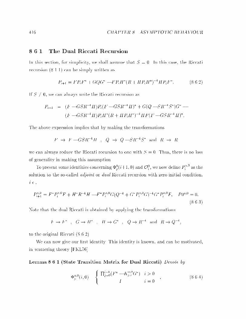
��� CHAPTER �� ASYMPTOTIC BEHAVIOUR
����� The Dual Riccati Recursion
In this section� for simplicity� we shall assume that S � �� In this case� the Riccati
recursion � ����� can be simply written as
Pi�� � FPiF� �GQG� � FPiH
��R �HPiH����HPiF
�� � �����
If S � �� we can always write the Riccati recursion as
Pi�� � �F �GSR��H�Pi�F �GSR��H�� �G�Q� SR��S��G� �
�F �GSR��H�PiH��R �HPiH
����HP �F �GSR��H���
The above expression implies that by making the transformations
F � F �GSR��H � Q � Q� SR��S� and R � R
we can always reduce the Riccati recursion to one with S � �� Thus� there is no loss
of generality in making this assumption�
To present some identities concerning ��p�i��� �� and O�
i � we now de�ne P a��i as the
solution to the so�called adjoint or dual Riccati recursion with zero initial condition�
i�e��
P a��i�� � F �P a��
i F �H�R��H � F �P a��i G�Q�� �G�P a��
i G���G�P a��i F� P�a�� � ��
� ����
Note that the dual Riccati is obtained by applying the transformations
F � F � � G� H� � H � G� � Q� R�� and R� Q���
to the original Riccati � ������
We can now give our �rst identity� This identity is known� and can be motivated�
in scattering theory �FKL����
Lemma ����� �State Transition Matrix for Dual Riccati� Denote by
�a��p �i� �� �
���Qi��j���F
� �Ka��p�i G
�� i � �
I i � �� � �����

���� CONVERGENCEOFTHE RICCATI RECURSIONWITHARBITRARYP����
the state transition matrix of F � �Ka��p�i G
�� Then we have
��p�i� ��� � �a��
p �i� ��� � �����
We shall defer the proof of Lemma ���� to the Appendix� For the time being� let
us note an important consequence of Lemma ���� that relates the state transition
matrices ��p�i� �� �corresponding to the zero�initial�condition solution of the Riccati
recursion� and �p�i� �� � �F�KpH�i�� �corresponding to any solution of the DARE��
Lemma ���� �Relation Between ��p�i� �� and �p�i� �� � �F �KpH�i��� We have
the following identity
��p�i� �� � �F �KpH�i
hI � PP
a��i
i� � �����
where
��p�i� �� � �F �K�
p�i��H� � � � �F �K�p��H�F
is the state transition matrix of F � K�p�jH corresponding to P �
j � the zero initial
condition solution to the Riccati recursion ����� P is any solution of the DARE
��� �� and P a��i is the zero initial condition solution to the dual Riccati recursion
Pa��i�� � F �P
a��i F � H�R��H � F �P
a��i G�Q�� �G�P
a��i G���G�P a��
i F� Pa��� � ��
Proof In this proof we assume that S � �� As mentioned earlier� the results readily
extend to the case S � �� Let us �rst note the identity
F �KpH � F � FPH��R�HPH���� � F �I � PH�R��H���� � �����
We now proceed to prove � ����� by induction� For i � � we have
��p��� �� � F�K�
p��H � F � F �I � PH�R��H���� z F�KpH
�I�P H�R��H� z Pa���
� � �F�KpH�hI � PP a��
�
i�

�� CHAPTER �� ASYMPTOTIC BEHAVIOUR
as desired�
Let us now suppose that � ����� is true for i� We then have
��p�i� �� �� � �a��
p �i� �� ��� � �a��p �i� ���F a���
p�i
� ��p�i� ��F a���
p�i
� �F �KpH�i�I � PPa��i �F a���
p�i � � ��� �
where we have twice made use of � ������ On the other hand� using the dual Riccati
recursion and an argument similar to � ����� we have
Fa��p�i � F ��I � P
a��i GQG�����
Using the above expression and proceeding with care yields
�I � PPa��i �F a���
p�i � �I � PPa��i ��I �GQG�P
a��i ���F
� �I � PPa��i �
���I � �P � F �I � PH�R��H���PF ��� z
GQG�
Pa��i
� ���
F
� �I � PPa��i ��I � PP
a��i � F �I � PH�R��H���PF �P a��
i ���F
� F � F �I � PH�R��H���� z F�KpH
PF �Pa��i �I � PP
a��i � F �I � PH�R��H���PF �P a��
i� z I�GQG�Pa��
i
���F
� F � �F �KpH�P F �Pa��i �I �GQG�P
a��i ���F� z
Pa��i���H
�R��H
� F � �F �KpH�P �P a��i�� �H�R��H�
� F � �F �KpH�PP a��i�� � F �I � PH�R��H���PH�R��H� z
F��F�KpH�
� �F �KpH�PP a��i�� � �F �KpH�
� �F �KpH��I � PPa��i����
If we now use the last of the above expressions in � ��� � we obtain
��p�i� �� �� � �F �KpH�i���I � PP a��
i����
which is the desired result�
Our next identity concerns O�i �
���� CONVERGENCEOFTHE RICCATI RECURSIONWITHARBITRARYP����
Lemma ����� �Identity for O�i � The quantity O�
i � de�ned in Lemma ���� � can be
expressed as
O�i � P
a��i��� � �����
Proof We begin by noting the identity
H��R�e�j�
��H � H��R�HP �j H
����H
� H�hR�� �R��H�I � P �
j H�R��H���P �
j H�R��
iH
�hI �H�R��H�I � P �
j H�R��H���P �
j
iH�R��H
�hI �H��R �HP �
j H����HP �
j
iH�R��H
�hF � �H��R �HP �
j H����HP �
j F�iF��H�R��H
� F ��p�iF
��H�R��H
Now plugging the last of the above equalities into � �� �� the expression for O�i � yields
O�i �
iXj��
��p�j� ���F ��
p�iF��H�R��H��
p�j� ��
�iX
j��
��p�j � �� ���F��H�R��H��
p�j� ��
�iX
j��
�a��p �j � �� ��F��H�R��H�a��
p �j� ���
�iX
j��
�a��p �j � �� ��H�R��H�a��
p �j� ���� � ������
On the other hand� using the dual Riccati recursion � ����� we may write
P a��i�� � P a��
i � F a��p�i �P a��
i � P a��i���F
a���p�i��
� �a��p �i� �� �� �P a��
� � Pa��� �� z
H�R��H
�a��p �i� ����
which implies that
Pa��i�� �
iXj��
�a��p �j � �� ��H�R��H�a��
p �j� ����
Comparing this last expression with � ������ yields the desired result�
��� CHAPTER �� ASYMPTOTIC BEHAVIOUR
��� Conditions on P� for Convergence
We now have most of the ingredients necessary to study the convergence of the solu�
tion of the Riccati recursion for an arbitrary initial condition P� � ��� by comparing
it with the zero�initial condition solution� P �i � However� in order to obtain explicit
conditions on P� for convergence� as opposed to the generic conditions of Theorem
����� we need to pay the price of specializing to the positive case� or the case where
Q � SR��S� � �� Although these may seem as restrictions� we should remark that
they are very important special cases and include the classes of Riccati recursions
encountered in both least�squares and H� estimation and control�
����� The Case Positive Case� R � � and Q � SR��S� � �
As frequently mentioned earlier� we may take S � �� so that our assumption becomes
R � � and Q � �� In this case� we can make further assertions regarding Pa��i the
zero�initial�condition solution to the dual Riccati recursion�
Lemma ����� �Monotonicity and Boundedness of P a��i � Consider the zero�initial�
condition dual Riccati recursion
Pa��i�� � F �P
a��i F �H�R��H � F �P
a��i G�Q�� �G�P
a��i G���G�P a��
i F� Pa��� � �
and suppose that Q � �� R � � and fF�GQ���g is stabilizable� Then we have the
following results�
�a The fP a��i g form a nondecreasing sequence of Hermitian matrices�
�b The fP a��i g are bounded from above� i�e�� there exists a Hermitian matrix � such
that
P a��i � ��
for all i � ��
Proof To prove the monotonicity we shall proceed by induction� For i � �� we have
Pa��� � H�R��H � � � P
a��� �

��� CONDITIONS ON P� FOR CONVERGENCE ���
Now suppose Pa��i � P
a��i��� We shall show P
a��i�� � P
a��i � To this end� let us apply
� ���� to the dual Riccati recursion and write
P a��i � P a��
i�� � F a��p�i��
h�P a��
i�� � P a��i �� �P a��
i�� � P a��i ��Ra��
e�i ����P a��i�� � P a��
i �iF a���p�i���
Now since P a��i � P
a��� � �� we have Ra��
e�i � R �HPa��i H� � �� Therefore both terms
on the RHS of the above expression are negative semi�de�nite� Thus� we can conclude
Pa��i�� � P
a��i �
which shows that the fP a��i g form a nondecreasing sequence of Hermitian matrices�
To prove boundedness� we shall use the stabilizability of fF�GQ���g� Since fF�GQ���g
is stabilizable� fF �� Q���G�g is detectable� meaning that we can choose a gain matrix
K such that F � �KQ���G� is stable� With this choice of K� we can write the dual
Riccati recursion as
Pa��i�� � �F ��KQ���G��P a��
i �F ��KQ���G����H�R��H�K�K��Ka��p�i �KQ����Ra��
e�i �Ka��p�i �KQ
������
Since F ��KQ���G� is stable� and H�R��H�K�K � �� there exists a unique positive
semi�de�nite solution� �� to the Lyapunov equation�
� � �F � �KQ���G����F � �KQ���G��� �H�R��H �K�K�
We shall now prove by induction that � is an upper bound on the sequence fP a��i g�
The case i � � is trivial since
� � � � Pa��� �
Suppose now that � � Pa��i � We shall show that � � P
a��i��� Indeed� subtracting the
Riccati recursion for P a��i from the Lyapunov recursion for �� yields
��P a��i�� � �F ��KQ���G�����P a��
i ��F ��KQ���G�����Ka��p�i �KQ����Ra��
e�i �Ka��p�i �KQ
������
Now both terms on the RHS of the above expression are positive semi�de�nite� This
implies that
� � Pa��i���
which is our desired result�

��� CHAPTER �� ASYMPTOTIC BEHAVIOUR
We can now make some further claims regarding the asymptotic behaviour of the
state transition matrix ��p�i� ���
Lemma ���� �Convergence of ��p�i� ��� If fF�Hg is detectable and fF�GQ���g
is stabilizable� then
limi��
��p�i� �� � �� � �����
Proof The proof uses the identity
��p�i� �� � �F �KpH�i
hI � PP
a��i
i�
established in Lemma ����� The desired result follows immediately from the fact
that the P a��i are bounded from above and below�
� � Pa��i � � ��� i � ��
and that F �KpH is stable so that
limi��
�F �KpH�i � ��
Let us now return to the identity � ����� and write it as
Pi�� � P �i�� � ��
p�i� �� ��hI � ��P
a��i��
i�����
�p�i� �� ���� � �����
where we have also used O�i � P
a��i��� Now� from Lemma ����� we know that when
fF�Hg is detectable and fF�GQ���g is stabilizable limi�� ��p�i� �� � �� Therefore
from � ����� we conclude that if the matrixhI � ��P
a��i��
i��is uniformly bounded for
all i� then
limi��
Pi�� � limi��
P �i�� � P�
In other words a su�cient condition for the convergence of Pi to P � the unique positive
semi�de�nite solution to the DARE is that the matrix
I � ��Pa��i � � ����
��� CONDITIONS ON P� FOR CONVERGENCE ��
be uniformly nonsingular for all i� We shall therefore continue by studying this matrix
in more detail�
Let us �rst suppose that �� � �� This is� of course� a natural assumption since
in estimation problems �� is the covariance matrix of the random initial state vector
x�� and in control problems it is the inverse of the positive weight matrix in the LQ
cost function associated with the initial state� In either case� we can perform the
factorization �� � ����� ����
� and write
det�I � ��Pa��i � � det�I � �
���� �
���� P
a��i �
� det�I � ����� P a��
i ����� �� � �����
where we have used the identity det�I �AB� � det�I � BA�� Now since P a��i is the
solution to the dual Riccati recursion � ���� with zero initial value� it is a positive
semi�de�nite matrix for all i� The same is therefore true of the congruent matrix
����� P
a��i �
���� � from which we conclude that I��
���� P
a��i �
���� is positive de�nite for all
i� Thus� in view of � ������ I � ��Pa��i is uniformly nonsingular for all i and we have
the following wellknown result �Wil��b� Kuc��� Won� a� BRC����
Lemma ����� �Convergence for P� � �� Consider the Riccati recursion with pos�
itive semi�de�nite initial condition
Pi�� � FPiF� �GQG� �Kp�iRe�iK
�p�i� P� � �� � �����
If Q � �� R � �� fF�Hg is detectable and fF � GSR��H�GQ � GSR��S�g is
stabilizable then Pi converges to the unique positive semi�de�nite matrix� P � that
satis�es the discrete�time algebraic Riccati equation
P � FPF � �GQG� � �FPH� �GS��R �HPH�����FPH� �GS���
Although the above result is quite satisfying� we still have not fully exploited the
condition that � ���� be uniformly nonsingular for all i � �� It would therefore be
interesting to explore whether it is possible to relax the nonnegativity condition on

��� CHAPTER �� ASYMPTOTIC BEHAVIOUR
��� while still guaranteeing convergence to P � We should note that this is not just
academic speculation since it will have certain implications for the numerical stability
of the Riccati recursion� Indeed� it will show that even if the Riccati variable Pi loses
its positive semi�de�niteness �due to say� numerical errors� it may still converge to
the solution of the DARE�
When �� is inde�nite it no longer yields a factorization of the form described
above� However� we can still factorize it as
�� � ����� J�
���� �
where J is a signature matrix whose diagonal elements represent the inertia �or num�
ber of positive and negative eigenvalues� of ���
We now have the following sequence of equalities�
det�I � ��Pa��i � � det�I � �
���� J�
���� P
a��i �
� det�I � J����� P a��
i ����� �
� det�J� � det�J � ����� P
a��i ����
� �� since J� � I�
Using the last of the above expressions� we see that � ���� is uniformly nonsingular if�
and only if� the Hermitian matrices Ti � J � ����� P
a��i ����
� are uniformly nonsingular
for all i � �� Since the matrices ����� P a��
i ����� are non�decreasing �P a��
i�� � P a��i �� the
matrices Ti are also non�decreasing� It also follows that all the eigenvalues of the
matrices Ti are non�decreasing as well� Therefore� a su�cient condition for the Ti
to be uniformly nonsingular for all i � �� is that all of the negative eigenvalues of
T� � J remain bounded above by zero as i increases� This� of course� means that the
matrices T� � J and the fTig should have the same inertia for all i � �� Moreover�
the fTig will have the same inertia as J for all i � � if� and only if�
limi��
Ti � T � J � ����� P a����
� � � �����
has the same inertia as J � �Note that P a� the limiting solution of the dual Riccati�
exists since we have assumed that fF�GQ���g is stabilizable��
We have therefore found a su�cient condition for checking whether � ���� is
uniformly nonsingular for all i � �� in terms of checking the inertia of a single matrix

��� CONDITIONS ON P� FOR CONVERGENCE ���
T � To facilitate checking the inertia of T � J � ����� P a����
� � consider the following
block matrix �� �I �P a�����
����
����� �P a���� J
�� � � �����
where we have de�ned P a � �P a�����P a����� Now two dierent �lower�upper and
upper�lower� block triangular factorizations of the above matrix yield
�� �I �
� T
�� and
�� �I � �P a�������P a���� �
� J
�� � � ��� �
Due to Sylvester�s law of inertia� the above two congruent matrices must have the
same inertia� Therefore the matrices T and J will have the same inertia if� and only
if� the matrices �I and �I� �P a�������P a���� have the same inertia� In other words�
if� and only if�
I � �P a�������Pa���� � ��
We thus have our desired result�
Theorem ����� �Convergence of Riccati Recursion with Inde�nite P�� Consider
the Riccati recursion
Pi�� � FPiF� �GQG� �Kp�iRe�iK
�p�i� P� � �����
where R � �� Q � SR��S� � �� fF�Hg is detectable and fF � GSR��H�GQ �
GSR��S�g is stabilizable� Suppose� moreover� that the initial condition P� is such
that
I � �P a����P��Pa���� � �� � ������
where P a is the unique positive semi�de�nite solution to the dual Riccati recursion�
Then Pi converges to the unique positive semi�de�nite matrix� P� that satis�es the
discrete�time algebraic Riccati equation
P � FPF � �GQG� � �FPH� �GS��R �HPH�����FPH� �GS���
��� CHAPTER �� ASYMPTOTIC BEHAVIOUR
The above result gives a very general description of the conditions for conver�
gence of the Riccati recursion in the positive case� Note that the detectability and
stabilizability conditions are the same as those required for the existence of a unique
stabilizing solution to the DARE �see Theorem ������� It is therefore not possible to
weaken these conditions very much� Detectability is a necessary condition since oth�
erwise the solution of the Riccati recursion may diverge to in�nity� If stabilizability
does not hold� then the DARE will have more than one positive semi�de�nite solution
and clearly if we start the recursion with one of these solutions we will always remain
at the same value� Therefore� there cannot be convergence to a unique value�
Moreover� � ������ gives a rather general description of the basin of attraction of
the positive semi�de�nite solution of the Riccati recursion� Under additional condi�
tions � ������ can be made more explicit� The result is given below� �The proof is
simple and is omitted��
Corollary ����� �Conditions for Convergence� When fF�Hg is observable� the
condition ������ is equivalent to
P� � ��P a���� � ������
Moreover� in this case we have
��P a��� � P��� the in�mum over all solutions to the DARE ������� � ������
Before closing this section� we should mention an interesting interpretation of the
condition � ������ required for the convergence of the Riccati recursion from a given
initial condition P��
Corollary ���� �Interpretation of Condition ��������� The condition
I � �P a����P��Pa���� � ��
su�cient for the convergence of the Riccati recursion from a given initial condition
P�� is equivalent to the condition that
Re�i � R �HPiH� � ��

��� CONDITIONS ON P� FOR CONVERGENCE ���
for all i � �� where Pi is the solution to the Riccati recursion with initial condition
P��
Proof The proof is similar to the proof of Theorem ����� part �b�� and is omitted
for brevity�
Note that the above result implies that we can check the positivity of the matrices
Re�i for all i � �� in terms of the positivity of a single matrix I � �P a����P��P a�����
However� more interesting is the stochastic interpretation of this result�
To this end� consider the stochastic state�space model��� xi�� � Fxi �Gui� i � �
yi � Hxi � vi� �����
where the fx��ui�vig are zero�mean random variables with Gramian �covariance�
matrices
h
�����x�
ui
vi
� � ������x�
uj
vj
� �i � E
�����x�
ui
vi
� ������x�
uj
vj
� ��
�
�����
�� � �
� Q S
� S� R
� � � � ������
Then it is wellknown �see e�g�� �Kai ��� that the Re�i are the Gramians of the� so�
called� innovations process� ei� associated with the state�space model � ����� �������
Therefore� the condition � ������ means that we can guarantee convergence for in�
de�nite �and even negative semi�de�nite� initial conditions� P� � ��� as long as the
innovations process associated with the state�space model � ����� ������ behaves as
a true stochastic process� i�e�� as one that has positive de�nite Gramian �covariance�
matrix� Finally� since the innovations ei are equivalent to the yi �in a stochastic
sense � see �Jaz��� AM��� Kai ���� we can guarantee convergence for all P� � �� for
which the output of the state�space model � ����� ������ behaves as a true stochastic
process�
����� The Case of Q � SR��S� � �
The special of case Q� SR��S� � � or� equivalently� of Q � �� �since we shall take
S � �� is of interest because it is the case that arises in H� �ltering and control� To

�� CHAPTER �� ASYMPTOTIC BEHAVIOUR
study the convergence in this case� we can begin with Eq� � ����� which we repeat
here for convenience�
Pi�� � P �i�� � ��
p�i� �� ��hI � ��P
a��i��
i�����
�p�i� �� ����
Using the generalized square�root of the initial condition �� � ����� J����
� � where J is
a signature matrix� we may write the above equation as
Pi�� � P �i�� � ��
p�i� �� �������
hJ � ����
� Pa��i���
����
i������� ��
p�i� �� ���� � ������
The following result is now immediate�
Lemma ����� �Comparison with Zero Initial Condition Solution� Consider the
Riccati recursion
Pi�� � FPiF� �GQG� � FPiH
��R �HPiH����HPF �� P� � ��
where Q � � and fF�GQ���g is stabilizable� Moreover� suppose that the associated
DARE has a unique stabilizing solution� P � and that the zero�initial�condition solution
P �i converges to P � Now if the matrices
Ti � J � ����� P
a��i���
����
are uniformly nonsingular for all i � �� where �� � ����� J����
� � and P a��i is the
zero�initial�condition solution to the dual Riccati recursion
P a��i�� � F �P a��
i F � H�R��H � F �P a��i G�Q�� �G�P a��
i G���G�P a��i F� P a��
� � ��
then Pi will converge to P � Two equivalent su�cient conditions for the Ti to be
uniformly nonsingular for all i � � are that
�a The matrices Ti have constant inertia for all i � ��
�b The matrices Re�i � R � HPiH� have constant inertia �equal to the inertia of
Re for all i � ��
��� CONDITIONS ON P� FOR CONVERGENCE ���
Proof To prove the �rst part of the Theorem we shall prove that
limi��
��p�i� �� � �� � ������
Once this is established� the convergence of Pi to P follows from � ������� sincehJ � �
���� P
a��i���
����
i��is bounded and P �
i converges to P �
To prove � ������ we can repeatedly use � ���� to write
P �i���P
�i � F �
p�i�P�i �P
�i���F
��p�i�� � ��
p�i��� ��P ����
p�i� ��� � ��p�i��� ��GQG���
p�i� ����
where we have used P �� � GQG�� Now we may write
�P �i�� � P �
i �F ��p�i � ��
p�i� �� ��GQG���p�i� �� ����
which� using Lemma ����� is equivalent to
�P �i�� � P �
i �F ��p�i � �a��
p �i� �� ���GQG��a��p �i� �� ���
This last expression can in turn be written as
F ��P �i�� � P �
i �F ��p�i � �a��
p �i� �� ���GQG��a��p �i� �� ���
and� using the facts that limi���P �i�� � P �
i � � � and Q � �� this implies that we
must have
limi��
Q���G��a��p �i� �� �� � �� � ������
The quantity �a��p �i� ��GQ��� is readily recognized to be the matrix that maps the
initial state to the output for the linear system
��� xi�� � �F � �Ka�o
p�iG��xi � �F � � F �P a��
i G�Ra��e�i ���G��xi
yi � Q���G�xi� � ���� �
Therefore� � ������ implies that yi tends to zero for all initial state vectors x�� But
� ���� � can be rewritten as
��� xi�� � F �xi � F �P
a��i G�Ra��
e�i ���Q����yi
yi � Q���G�xi�

�� CHAPTER �� ASYMPTOTIC BEHAVIOUR
and since fF �� Q���G�g is detectable �fF�GQ���g is stabilizable�� yi cannot tend to
zero unless xi tends to zero as well� Hence� the state transition matrix
�a��p �i� �� � ��
p�i� ����
tends to zero as i��� �This is just a reformulation of the fact that output feedback
cannot destroy detectability � see e�g�� �Kai ����
To prove the second part� we note that if the Ti have constant inertia �equal to
the inertia of J� for all i � �� then they will be uniformly nonsingular as well� Finally�
the equivalence of the su�cient conditions �a� and �b� is the same as the proof for
Theorem �����
Remarks
�i� Note that in the above Lemma we still require to check the uniform nonsingu�
larity� or constant inertia� of the sequence of matrices Ti � J � ����� P
a��i���
���� �
We saw in the positive case that we could replace checking the inertia of the
above in�nite sequence of matrices with checking the inertia of a single matrix�
This was possible because we were able to show that in the positive case the
sequence of matrices P a��i were nondecreasing� Since in the case where Q � ��
it is not generally true that the P a��i are nondecreasing� it does not seem that
we can replace the checking of the inertia of the sequence of matrices fTig with
that of a single matrix� Indeed we have not been able to do so�
�ii� The su�cient condition �b� in Lemma ���� has an interesting interpretation
since it is the exact condition that is required for the existence of H� �lters
or full information controllers �see e�g�� �GL��� HSK��b��� Therefore� if a time�
varying H� �lter� or full information controller� exists for all times i � �� then
the corresponding Riccati recursion converges� meaning that the time�varying
H� �lter� or controller� will converge to a time�invariant one�
Despite the result of the preceding Lemma� it is still possible to give some simple
description of the basin of attraction of the Riccati recursion when Q � �� However�

��� CONDITIONS ON P� FOR CONVERGENCE ��
to do so we need to take a slightly dierent line of attack� The approach used� follows
the one presented in the proof of Theorem ����� and the result is given below�
Theorem ���� �Conditions on P� for Convergence in the Q � � Case� Consider
the Riccati recursion
Pi�� � FPiF� �GQG� � FPiH
��R �HPiH����HFPiF
�� P�� � ������
where
R �
�� Ip� �
� �Ip�
�� � H �
�� H�
H�
�� �
fF�H�g is detectable� fF�GQ���g is stabilizable and Q � �� Suppose� moreover� that
the DARE
P � FPF � �GQG� � FPH��R �HPH����HPF �� � ������
has a stabilizing solution� P � such that the matrices R and Re � R�HPH� have the
same inertia� Then if the initial condition� P�� is such that
� � P� � ��
where � is the unique positive �semide�nite solution of the Lyapunov equation�
� � F�F � �GQG��
the sequence of matrices fPig will converge to P �
Proof Note that due to Theorem ����� since P is the stabilizing solution to the
DARE it is positive semi�de�nite� Now sinceR andRe have the same inertia� Theorem
���� says that the matrix F �K�H is stable� where
K� � FPH�� �Ip� �H�PH
�� ����
Now if we assume that fF�GQ���g is controllable� then the Lyapunov equation�
� � F�F � � GQG�� equation implies that � � �� �We should remark that the
controllability assumption is for simplicity and that the end result does not require
this assumption��
�� CHAPTER �� ASYMPTOTIC BEHAVIOUR
Moreover� from the proof of Theorem ���� for all times i � �� we may writeP�j��� j�sjj�P��
j��� jujj� �P��
j��� jvjj� �Pi
j�� jujj� �
Pij�� jvjj
�� �� � ������
where �si � si � �si is the estimation error associated with estimating si �using some
estimator that will not concern us here� from the observations fyjgij���� and where
si and yi have the state�space model���������xi�� � Fxi �GQ���
yi � H�xi � vi
si � H�xi
� ������
Now for all nonzero sequences fujg and fvjg� we may write � ������ as�� ��Xj���
jujj� �
��Xj���
jvjj� �
��Xj���
j�sjj�
�A �
�� iXj��
jujj� �
iXj��
jvjj� �
�Xj��
j�sjj�
�A � ��
� �����
Now let us �x an initial state x� and choose the sequence fuj� vjg��j��� such that
fumj � vmj g
��j��� � argminfuj�vjg
�� ��Xj���
jujj� �
��Xj���
jvjj�
�� � � ������
where the fuj� vj� �sjg satisfy the state�space constraints
xi�� � Fxi �GQ���� �� � i � � � ������
and generate the initial state vector x�� The solution to the above minimization
problem is wellknown in quadratic game theory and LQR control �see e�g�� �AM���
KS��� BO ���� For our purposes it su�ces to know that the value of the LQ �linear
quadratic� cost function at its minimum is given by
��Xj���
jumj j� �
��Xj���
jvmj j�� � min
fuj �vjg
�� ��Xj���
jujj� �
��Xj���
jvjj��
�� � x���
��x��
where � is the solution to the Lyapunov equation� � � F�F � �GQG��
With this particular choice of inputs� we may write � ����� as
x�����x� �
iXj��
jujj� �
iXj��
jvjj� �
�Xj���
j�sjj� � ��

���� CONCLUSION �
or� P�j��� j�sjj�
x�����x� �
Pij�� jujj
� �Pi
j�� jvjj�� ��
and after discarding that portions of the numerator that involve j � i and j � ��
Pij�� j�sjj
�
x�����x� �Pi
j�� jujj� �
Pij�� jvjj
�� �� � ������
Note that in the above inequality the fx�� fujgij��� fvjgij��g are arbitrary� Moreover�
it also readily follows that in the above relation we can replace P�� with any matrix
P��� such that
P��� � ����
and write Pij�� j�sjj
�
x��P��� x� �
Pij�� jujj
� �Pi
j�� jvjj�� �� � ������
Now from Lemma �A�� in the Appendix� we can conclude that the matrices
Re�j � R �HPjH��
must have constant inertia for all � � j � i� where Pj satis�es the Riccati recursion
� ������� Now since the above is true for all i � �� we conclude that with this choice of
initial condition the matrices Re�i must have constant inertia for all i � �� Therefore�
using the result of Theorem ����� we see that for all initial conditions such that
� � P� � ��
the solution to the Riccati recursion� Pi� will converge to the unique stabilizing solu�
tion� P �
��� Conclusion
In this chapter we studied the asymptotic behaviour of the Riccati recursion for time�
invariant state�space models� The main result is a general inertia condition for the

�� CHAPTER �� ASYMPTOTIC BEHAVIOUR
convergence of the Riccati recursion variable to the unique stabilizing solution of the
associated DARE �assuming such a solution exists�� We also gave some more simple
and more explicit conditions in the special cases encountered in LQR and H� control�

��A� FINITEHORIZON H� PROBLEMS ��
��A Finite�Horizon H� Problems
We begin by proving a Lemma that was used in the proof of Theorem ����� This
Lemma is wellknown in H� theory �see e�g�� �GL��� HSK��b� and Chapter � and is
given below�
Lemma ��A�� �Finite Horizon H� Filtering� Consider the state�space model
��� xj�� � Fxj �GQ���uj� � � j � i
yj � H�xj � vj
where the fx�� fujgij��� fvjgij��g are unknown and the fyjgij�� are known measure�
ments� Suppose we would like to estimate the linear combination of the states�
sj � H�xj�
using the observations fykgjk��� and designate this estimate by �sj� If it is possible to
choose the estimates f�sjgij�� such that
Pij�� jsj � �sjj�
x��P��� x� �
Pij�� jujj
� �Pi
j�� jvjj�� �� � �A���
for all fx�� fujgij��� fvjgij��g� then the matrices
Re�j � R �HPjH��
will have constant inertia for all � � j � i� where Pj satis�es the Riccati recursion
Pj�� � FPjF� � GQG� � FPjH
��R�HPjH����HPjF
�� P��
and
R �
�� Ip� �
� �Ip�
�� � H �
�� H�
H�
�� �
To prove the above Lemma� it will be useful to �rst establish the following inter�
mediate result�

�� CHAPTER �� ASYMPTOTIC BEHAVIOUR
Lemma ��A� �Minimization of Inde�nite Quadratic Forms� Consider the quadratic
form
Ji � x��P��� x� �
iXj��
u�jQ��j uj �
iXj��
v�jR��j vj�
where the fx�� fujgij��� fvjgij��g satisfy the state�space constraints��
� xj�� � Fxj �Guj� x�� � � j � i
yj � Hxj � vj� �A���
and where the fP�� fQjgij��� fRjgij��g are �possibly inde�nite Hermitian matrices of
the appropriate dimensions� Then� if P� � � and Qj � �� for j � �� � � � i� the Ji will
recursively have minima over the free variables fx�� fujgij��g for all i � �� if� and
only if� the matrices
R and Re�i � R �HPiH� � �A��
have the same inertia for all i � �� where Pi satis�es the Riccati recursion
Pi�� � FPiF� �GQG� � FPiH
��R�HPiH����HPiF
�� P��
Proof To prove the Lemma let us introduce the notation
u �
�����u����
ui
� � �
�����v����
vi
� � �
�����y����
yi
� �
and
Q � Q� � � � ��Qi � R � R� � � � ��Ri
along with the observability and impulse response matrices
O �
���������
H
HF���
HF i
� �
and � �
������������
�
HG �
HFG HG���
���� � �
HF i��G HF i��G � � � �
� ��

��A� FINITEHORIZON H� PROBLEMS ��
With these de�nitions� we may write the state�space equations � �A��� in global form
as
y � Ox� � �u � v�
and the quadratic cost function as
Ji � x��P��� x� � u�Q��u� v�R��v
� x��P��� x� � u�Q��u� �Ox� � �u� v�R���Ox� � �u� v��
�h h
x�� u�i
y�i����
�P���
Q��
��
�O
�
�R��
hO� ��
i�
�O
�
�R��
�R��hO� ��
iR��
� ������x�
u
�
y
� � �
Using this last expression� we readily see that Ji has a minimum over fx�� ug if� and
only if�
M �
�� P��� �
� Q��
���
�� O
�
��R�� h O� ��
i� ��
Now consider the matrix
T �
������� P��� �
� Q��
��
�� O
�
��
hO� ��
i�R
� � �
Two dierent �upper�lower and lower�upper� block triangular factorizations of T show
that the matrices
�� M �
� �R
�� and
�������
�� P��� �
� Q��
�� �
� ��R�OP�O� � �Q��� z
Ry
�
� �
are congruent and therefore must have the same inertia� But since
�� P��� �
� Q��
�� � ��
we conclude that M � � if� and only if the matrices R and Ry have the same inertia�
Now using the theory of Kalman �ltering in Krein spaces �the natural extension of
classical Kalman �ltering to inde�nite metric spaces � see �HSK��c� HSK��b� and
Chapter �� we can perform the �block� triangular factorization of Ry as follows
Ry � LReL��

� CHAPTER �� ASYMPTOTIC BEHAVIOUR
where L is lower triangular with unit diagonal� and
Re � Re�� � � � ��Re�i�
with Re�j given by � �A��� Thus M � � �and Ji has a minimum over fx�� ug� if� and
only if� Re and R have the same inertia� But since we require that Ji have a minimum
over fx�� fujgij��g for all i � �� this means that the block diagonal entries of Re and
R i�e�� the matrices Re�i and R� must have the same inertia for all i � ��
Proof of Lemma ��A�� We �rst note that if � �A��� is true� then for all i � � we
must have
x��P��� �
iXj��
u�juj �iX
j��
v�jvj �iX
j��
��sj � sj����sj � sj� � ��
for all fx�� fujgij��� fvjgij��g� subject to the state�space constraints� Now the above
quadratic form can be rewritten in the more familiar form
x��P��� �
iXj��
u�juj �iX
j��
�
�� yj
�sj
���
�� H�
H�
��xj��
�� Ip� �
� �Ip�
�� �
�� yj
�sj
���
�� H�
H�
��xj� � ��
� �A���
Now if the above quadratic form is to be positive for all fx�� fujgij��� fvjgij��g it must
have a minimum over the free variables fx�� fujgij��g �otherwise the fx�� fujgij��g can
be chosen to make the quadratic form arbitrarily negative�� By de�ning
H �
�� H�
H�
�� and R �
�� Ip� �
� �Ip�
��
we can readily identify the above quadratic form with the Ji of Lemma �A��� Since
the above quadratic form should have a minimum for all i � �� we may apply the
result of Lemma �A�� to conclude that the matrices
R and Re�i
must have the same inertia for all i � �� which is the desired result�

��B� PROOF OF LEMMA ����� ��
��B Proof of Lemma ����
In this section we shall provide a proof for the identity
��p�i� ��� � �a��
p �i� ��� � �B���
This identity can be motivated through scattering theory �FKL���� Here we shall give
an algebraic proof that also sheds further light on the Riccati recursion and brings
forth certain concepts related to scattering theory �namely� the Hamiltonian matrix��
In what follows we shall assume� without loss of generality� that S � � �see the
discussion at the beginning of Sec� ������ We shall also assume� for simplicity� that
F is invertible� although the �nal result� i�e� � �B���� does not require the invertibility
of F �see also �FKL�����
We begin by writing the Riccati recursion as
Pi�� � FPiF� �GQG� � FPiH
��R�HPiH����HPiF
�
� FhI � PiH
��R�HPiH����H
iPiF
� �GQG�
� F �I � PiH�R��H���PiF
� �GQG��
The above equation we can write as
�I � PiH�R��H�F���Pi�� �GQG�� � PiF
��
or after some simpli�cation
F��Pi�� � PiH�R��F��Pi�� � F��GQG� � PiH
�R��HF��GQG� � PiF� � ��
Gathering terms yields
hI �Pi
i�� F�� �F��GQG�
�H�R��HF�� F � �H�R��HF��GQG�
���� Pi��
I
�� � � �B���
The center matrix appearing in the above expression is referred to as the Hamiltonian
matrix and is denoted by
M �
�� F�� �F��GQG�
�H�R��HF�� F � �H�R��HF��GQG�
�� � � �B��

��� CHAPTER �� ASYMPTOTIC BEHAVIOUR
It is convenient to expand the block row and column vectors appearing in � �B���
into upper triangular matrices� to obtain�� I �Pi
� I
���� F�� �F��GQG�
�H�R��HF�� F � �H�R��HF��GQG�
���� I Pi��
� I
�� �
Due to � �B���� the ��� �� block entry in the above resulting product is zero� Some
simple algebra shows that the remaining block entries are�� I �Pi
� I
��M
�� I Pi��
� I
�� �
�� F��p�i �
�H�R��HF�� F �p�i
�� � � �B���
We now consider the product
iYj��
�� I �Pj
� I
��M
�� I Pj��
� I
�� �
Since �� I �Pj
� I
�� �
�� I Pj
� I
���� �
we readily see
iYj��
�� I �Pj
� I
��M
�� I Pj��
� I
�� �
�� I �P�
� I
��M i��
�� I Pi��
� I
�� �
On the other hand� using � �B���
iYj��
�� I �Pj
� I
��M
�� I Pj��
� I
�� �
�� �p�i� �� ���� �
� �
�� �
where �� denotes irrelevant entries�
We thus have the following identity�� I �P�
� I
��M i��
�� I Pi��
� I
�� �
�� �p�i� �� ���� �
� �
�� �
In particular� if we choose P� � �� we have
M i��
�� I P �
i��
� I
�� �
�� ��
p�i� �� ���� �
� �
�� �

��B� PROOF OF LEMMA ����� ���
which implies hM i��
i��
� ��p�i� �� ����� � �B���
where �M i����� denotes the ��� �� block entry of M i���
In a similar fashion� if one starts with the dual Riccati recursion
P ai�� � F �P a
i F � H�R��H � F �P ai G�Q�� �G�P a
i G���G�P ai F�
then it turns out that the dual Hamiltonian matrix Ma is simply
Ma � M��
Moreover� the analog of � �B��� is
h�Ma�i��
i��
�h�M��i��
i��
�hM i��
i���
� �a��p �i� �� ����� � �B���
Comparing � �B��� and � �B��� yields
�a��p �i� �� �� � ��
p�i� �� ����
which is the desired result�

��� CHAPTER �� ASYMPTOTIC BEHAVIOUR
��C Some Global Expressions
In this section we shall give some global expressions for the solution to the Riccati
recursion and for various related quantities� Although the material presented here is
of interest in its own right� it is also useful in giving alternative derivations of some
of the results presented in the chapter that implicitly assumed the invertibility of the
state transition matrix� F � �We should remark that none of the results given in this
chapter require this invertibility assumption� They were made primarily to streamline
the arguments that appeared in the main body of the chapter��
We also remark that the presentation given here is purposefully brief� The active
�and interested� reader should be able to �ll in the details�
We begin by noting that the standard state�space model can be written in global
form as ��� xi�� � �x� � Cu �
y � Ox� � �u � v �� �C���
where
y �
�����y����
yi
� � � u �
�����u����
ui
� � � v �
�����v����
vi
� � � � �C���
with
h
�����x�
u
v
� � ������x�
u
v
� �i �
�����
�� � �
� Q �
� � R
� � �
Q � diag�Q� � � �Q� �
R � diag�R� � � � R� �� �C��
and where � � F i is the state transition matrix�
O �
���������
H
HF���
HF i��
� �
and C �hF i��G F i��G � � � G
i� � �C���

��C� SOME GLOBAL EXPRESSIONS ��
are the observability and controllability maps� and
� �
������������
� � � �
HG � � �
HFG HG � �
HF �G HFG HG ����
������
� � �
� �� � �C���
is the impulse response matrix�
Now using the de�nition of Pi���
Pi�� � hxi���xi��i � hxi���yihy�yi��hy�xi��i� � �C���
it is possible to show the following result�
Lemma ��C�� �Global Expression for Pi� We have the following identity�
Pi�� �h
� Ci��
�� ���
� �
� Q��
���
�� O�
��
��R��
hO �
i�A���� ��
C�
�� � � �C���
In particular� when �� � ��
P �i�� � C
hQ�� � ��R���
i��C�� � �C� �
Similarly� using the de�nition �xi�� � hxi���yihy�yi��y� we can show that
�xi�� � ����O� � CQ����R �O��O
� � �Q������Ox� � �u� v�� � �C���
Now writing a global expression for �xi�� � xi����xi�� one can deduce that �p�i��� ���
the mapping from x� to �xi��� is given by the following result�
Lemma ��C� �Global Expression for �p�i� �� ��� We have the following iden�
tity�
�p�i� �� �� � � � ����O� � CQ����R�O��O
� � �Q�����O� � �C����
In particular� when �� � ��
��p�i� �� �� � � � CQ���R � �Q�����O� � �C����
��� CHAPTER �� ASYMPTOTIC BEHAVIOUR
Using a similar �actually dual� argument allows us to write�
�a��p �i� �� �� � �� �O�R����Q�� � ��R������C�� � �C����
But the identity�
Q���R� �Q����� � �Q�� � ��R��������R���
implies that
�a��p �i� �� �� � ��
p�i� �� ���� � �C���
which is an alternative proof of Lemma ���� that does not require the invertibility
of F �
��C�� Alternative Proof of Lemma ����
We shall now outline the steps of a �global� alternative proof of the identity
P a��i�� �
iXj��
��p�j� ���H��R�
e�j���H��
p�j� ��� � �C����
To do so� we begin �with an argument similar to what led to Lemma �C��� to
write
Pa��i�� � O� �R � �Q�����O� � �C����
In order to write the above result as a sum� we can perform the triangular factorization
of the output Gramian matrix
Ry � R � �Q�� � LR�eL
�� � �C����
with L lower triangular with unit diagonal and R�e �block� diagonal� We thus have
P a��i�� � O�L���R�
e���L��O� � �C����
Moreover� it is easy to see that the nonzero entries of the i�th column of L �where we
begin counting the columns from zero� are given by
li �
������������
I
HK�p�i
HFK�p�i
HF �K�p�i
���
� �� � �C�� �

��C� SOME GLOBAL EXPRESSIONS ���
The readily veri�ed identity�
O � L
���������
H
HFp��
HFp��Fp�����
� �� � �C����
now yields the desired result�
��C�� Alternative Proof of Lemma ����
We �rst use Lemma �C�� to write
P���i�� � P
���i�� �
h� C
i ��A� �A��� �A
� �� ��
C�
�� � � �C����
where we have de�ned
A �
�� ��
���� ��� �
� Q��
���
�� O�
��
��R��
hO �
iand �A �
�� ��
���� ��� � ��
���� ��� �
� �
�� �
� �C����
Now de�ning the following factorization of �A�
�A �
�� B
�
��J h B� �
i� � �C����
where B is full rank and J is an appropriate inertia matrix� allows us to write
P���i���P
���i�� �
h� C
iA��
�� B
�
����J �
hB� �
iA��
�� B
�
���A�� h B� �
iA��
�� ��
C�
�� �
� �C���
Now using� the readily veri�ed facts that
h� C
iA�� �
h����p �i� �� ���
���� �
i� � �C����
where � denotes irrelevant entries� and
hB� �
iA��
�� B
�
�� � B���
���� ��
���� O�R��y O�
���� �B� � �C����

��� CHAPTER �� ASYMPTOTIC BEHAVIOUR
where Ry�� R �O��O� � �Q��� allows us to write�
P���i���P
���i�� � ����
p �i��� ������� B
hJ �B������
� ������ O�R��y O����
� �Bi��
B������ ����
p �i��� ����
and� upon further simpli�cation�
P���i�� � P
���i�� � ����
p �i� �� ��hI � �����
� ������ �O�R��y O
i�������
� ������ �����
p �i� �� ����
� �C����
Now an argument similar to what was presented in Sec� �C�� allows us to conclude
O�R��y O �iX
j��
����p �j� ���H��R���
e�j ���H����
p �j� ��� � �C����
But this is the same as the expression given for O���i � given in Lemma ���� and we
have therefore established the identity
P���i�� � P
���i�� � ����
p �i� �� ��hI � �����
� ������ �O���
i
i�������
� ������ �����
p �i� �� ����
� �C�� �
which is our desired result�

Chapter �
H� Optimality of the LMS
Algorithm
In this chapter we show that the celebrated LMS �least�mean�squares� adaptive algo�
rithm is H� optimal� The LMS algorithm has been long regarded as an approximate
solution to either a stochastic or a deterministic least�squares problem� and it es�
sentially amounts to updating the weight vector estimates along the direction of the
instantaneous gradient of a quadratic cost function� In this chapter we show that
LMS can be regarded as the exact solution to a minimization problem in its own
right� Namely� we establish that it is a minimax �lter� it minimizes the maximum
energy gain from the disturbances to the predicted errors� while the closely related
so�called normalized LMS algorithm minimizes the maximum energy gain from the
disturbances to the �ltered errors� Moreover� since these algorithms are centralH� �l�
ters� they minimize a certain exponential cost function and are thus also risk�sensitive
optimal� We discuss the various implications of these results� and show how they pro�
vide theoretical justi�cation for the widely observed excellent robustness properties
of the LMS �lter�

� CHAPTER �� H� OPTIMALITY OF THE LMS ALGORITHM
��� Introduction
Classical methods in estimation theory �such as maximum�likelihood� maximum en�
tropy and least�squares� require a priori knowledge of the statistical properties of the
exogenous signals� In many applications� however� one is faced with model uncer�
tainties and lack of statistical information� Therefore� the introduction of the LMS
�least�mean�squares� adaptive �lter by Widrow and Ho� in ��� came as a signi�cant
development for a broad range of engineering applications since the LMS adaptive
linear�estimation procedure requires essentially no advance knowledge of the signal
statistics �WH���� Since this pioneering work� adaptive �ltering techniques have been
widely used to cope with time variations of system parameters and lack of a priori
statistical information �WS��� Hay����
The LMS algorithm was originally conceived as an approximate recursive proce�
dure that solves the following least�squares adaptive problem� given a sequence of
�n input row vectors fhig� and a corresponding sequence of desired responses fdig�
�nd an estimate of an n� column vector of weights w� such that the sum of squared
errorsPN
i��jdi�hiwj� is minimized� The LMS solution recursively updates estimates
of the weight vector along the direction of the instantaneous gradient of the squared
error�
Algorithms that exactly minimize the sum of squared errors� for every value of
N � are also known and are generally referred to as recursive least squares �RLS�
algorithms �see� e�g�� �Hay��� SK�b��� Although such exact least�squares algorithms
have various desirable optimality properties �such as yielding maximum likelihood
estimates� under certain statistical assumptions on the signals �such as temporal
whiteness and Gaussian disturbances�� they are computationally more complex� and
are less robust to disturbance variation than the simple LMS algorithm� For example�
it has been observed that the LMS algorithm has better tracking capabilities than
the RLS algorithm in the presence of nonstationary inputs �Hay����
In this chapter we show that the superior robustness properties of the LMS al�
gorithm are due to the fact that it is a minimax algorithm� or more speci�cally an
H� optimal algorithm� We shall de�ne precisely what this means in Sec� ���� Here

���� INTRODUCTION �
we note only that recently� following some pioneering work in robust control theory
�see� e�g�� �Zam� �� there has been an increasing interest in minimax estimation �see
Sec� � and Chapter � and the references therein� with the belief that the resulting
so�called H� algorithms will be more robust and less sensitive to model uncertainties
and parameter variations� The similarity between the objectives of adaptive �ltering
and H� estimation suggests that there should be some connection between the two�
and indeed our result on the H� optimality of the LMS algorithm provides such a
connection�
In addition to giving more insight into the inherent robustness of the LMS algo�
rithm� and why it has found such wide applicability in a diverse range of problems�
our result provides LMS with a rigorous basis and furnishes a minimization criterion
that has long been missing� To be more precise� using some well�known results in H�
estimation theory� we show that the LMS algorithm is the so�called central a priori
H��optimal �lter� while the closely related normalized LMS algorithm is the central
a posteriori H��optimal �lter�
The H� optimality property of LMS is a deterministic characterization of the
algorithm� It is also possible to give a stochastic characterization of this algorithm
under the assumptions of temporal whiteness and Gaussian disturbances� In this
case� we show that LMS minimizes the expected value of a certain exponential cost
function� and is therefore risk�sensitive optimal �in the sense of Whittle �Whi�����
It is ironic that the LMS algorithm is not H� optimal� contrary to what its name
suggests� but that it rather satis�es a minimax criterion� Moreover� in most H�
problems� the optimum solution has not been determined in closed form � what is
usually determined is a certain type of suboptimal solution� We show� however� that
for the adaptive problem at hand� the optimum solution can be determined�
The remainder of the chapter is organized as follows� In Sec� ��� we introduce the
problem of adaptive �ltering and motivate the question of the robustness of estima�
tors� In order to address the robustness question� we introduce the H� approach in
Sec� ��� and formulate the H� estimation problem as one that minimizes the max�
imum energy gain from the disturbances to the estimation errors�� Sec� �� closely
�The presentation of Secs� ��� and ��� closely follows that of Sec� ���� but is included to keep

�� CHAPTER �� H� OPTIMALITY OF THE LMS ALGORITHM
follows Sec� ��� and studies the general problem of state�space H� estimation and�
in particular� gives expressions for the H� a posteriori and a priori �lters� as well
as their full parametrization� The main result is given in Sec� ��� where we formu�
late the H� adaptive �ltering problem as a state�space problem and use the results
of Sec� �� to show that the normalized LMS algorithm is the central a posteriori
H� optimal adaptive �lter� and that� if the learning rate is chosen appropriately�
LMS is the central a priori H� optimal adaptive �lter� In both cases� the LMS and
normalized LMS algorithms guarantee that the energy of the estimation errors never
exceeds the energy of the disturbances� Sec� ��� then considers a simple example that
demonstrates the robustness of LMS compared to RLS� and also brie�y discusses the
merits of being H��optimal� In Sec� �� the full parametrization of all H� optimal
adaptive �lters is given� and in Sec� ��� we show that LMS and normalized LMS
have the additional property of being risk�sensitive optimal� Sec� ��� mentions some
further results using the approach and ideas of this thesis and Sec� �� � provides the
conclusion�
��� Adaptive Filtering
As shown in Fig� �� � suppose we observe an output sequence fdig that obeys the
following model�
di � hiw � vi� i � � ����� �
where hi �hhi� hi� � � � hin
iis a known �n input vector� w �
hw� w� � � � wn
iTis an unknown n� weight vector that we intend to estimate� and vi is an unknown
disturbance� which may also include modeling errors� We shall not make any assump�
tions on the noise sequence fvig �such as stationarity� whiteness� Gaussian distributed�
etc��� We denote the estimate of the weight vector using all the information available
up to time i by
�wji � F�d�� d�� � � � � di�h�� h�� � � � hi��
the chapter selfcontained�

���� ADAPTIVE FILTERING �
��������
����
����� �
� �
�
��
�
� �
hi� h�� hi� hin
vi
di hiw � viw� w� w� wn
Figure �� � The model for adaptive �ltering�
����� Least�Squares Methods
There are a variety of choices for �wji� but the most widely used estimate is one that
satis�es the following least�squares �or H�� criterion�
minw
�����jw � �wj��j
� �iX
j��
jdj � hjwj�
�� � �������
where �wj�� is the initial estimate of w� and � � � represents the relative weight
that we give to our initial estimate compared to the �sum of squared�error� termPij�� jdj � hjwj��
The exact solution to the above criterion is the RLS �recursive least squares�
algorithm�
�wji � �wji�� � kp�i�di � hi �wji��� � �wj�� �������
with kp�i �Pih
�i
��hiPih�i
and Pi satisfying the Riccati recursion
Pi�� � Pi �Pih
�ihiPi
� hiPih�i� P� � �I� ������
The RLS algorithm is used because under suitable stochastic assumptions it has
the following two properties��
�a� If w� �wj�� and the fvjg are assumed to be zero�mean� uncorrelated and� in the
case of the fvjg� temporally white random variables with variances �I and �
�See e�g�� Sec� ����
�� CHAPTER �� H� OPTIMALITY OF THE LMS ALGORITHM
respectively� then the RLS algorithm minimizes the expected prediction error
energy�
EiX
j��
jhjw � hjwj��j��
�b� If� in addition to the assumptions of part �a�� w� �wj�� and the fvjg are assumed
to be jointly Gaussian� then the cost function in ������� becomes the negative
of the log�likelihood function and RLS yields the maximum�likelihood estimate
of the weight vector w�
����� Gradient�Based Methods
In gradient�based algorithms� instead of exactly solving the least�squares problem
�������� the estimates of the weight vector are updated along the negative direction of
the instantaneous gradient of the cost function appearing in �������� Two examples
are the LMS �Least�Mean�Squares� �WH���
�wji � �wji�� � �h�i �di � hi �wji��� � �wj�� �������
and the normalized LMS
�wji � �wji�� ��
� �hih�ih�i �di � hi �wji��� � �wj�� �������
algorithms� Note that in the case of LMS the gain vector kp�i in RLS �which had to
be computed by propagating a Riccati equation� has been simply replaced by �h�i �
Likewise if we compare normalized LMS with the RLS algorithm� we see that the
di�erence is that instead of propagating the matrix Pi via the Riccati recursion we
have simply set Pi � �I� for all i� For this reason the LMS and normalized LMS
algorithms have long been considered to be approximate least�squares solutions and
were thought to lack a rigorous basis�
We should note here that although we have introduced the LMS algorithm as an
approximate deterministic least�squares solution� it is also possible to motivate it as
an approximate stochastic least�squares solution �see �WS��� Hay�����

���� THE H� APPROACH ��
����� The Question of Robustness
We saw that under suitable stochastic assumptions� the RLS algorithm has certain
desirable optimality properties� namely it minimizes the expected prediction error
energy and yields maximum�likelihood estimates� However� the question that begs
itself is what the performance of such an estimator will be if the assumptions on the
disturbances are violated� or if there are modeling errors in our model so that the
disturbances must include the modeling errors� In other words
� is it possible that small disturbances and modeling errors may lead to large
estimation errors�
Obviously� a nonrobust algorithm would be one for which the above is true� and a
robust algorithm would be one for which small disturbances lead to small estimation
errors� More explicitly� in the adaptive �ltering problem� where we assume an FIR
model� the true model may be IIR� but we neglect the tail of the �lter response since
its components are small� However� unless one uses a robust estimation algorithm� it
is conceivable that this small modeling error may result in large estimation errors�
The problem of robust estimation is thus an important one� As we shall see
in the next section� the H� estimation formulation is an attempt at addressing this
question� The idea is to come up with estimators that minimize �or in the suboptimal
case� bound� the maximumenergy gain from the disturbances to the estimation errors�
This will guarantee that if the disturbances are small �in energy� then the estimation
errors will be as small as possible �in energy�� no matter what the disturbances are�
In other words the maximum energy gain is minimized over all possible disturbances�
The robustness of the H� estimators arises from this fact� Since they make no
assumption about the disturbances� they have to accommodate for all conceivable
disturbances� and thus may be over�conservative�
��� The H� Approach
We begin with the de�nition of the H� norm of a transfer operator� As will presently
become apparent� the motivation for introducing theH� norm is to capture the worst
� CHAPTER �� H� OPTIMALITY OF THE LMS ALGORITHM
case behaviour of a system��
De�nition ����� �The H� Norm� Let h� denote the vector space of square�summable
complex�valued causal sequences with inner product � ffkg� fgkg � �P�
k�� f�k gk �
where � denotes complex conjugation� Let T be a transfer operator that maps an input
sequence fuig to an output sequence fyig� Then the H� norm of T is de�ned as
kT k� � supu ����u�h�
kyk�
kuk�
where the notation kuk�denotes the h��norm of the causal sequence fukg� viz��
kuk���P�
k�� u�kuk�
Note that the H� norm may thus be regarded as the maximum energy gain from
the input u to the output y�
����� Formulation of the H� Adaptive Filtering Problem
Recall that �wji � F�d�� � � � di�h�� � � � hi� denotes the estimate of the weight vector
using all the information available from time � to time i� In this chapter we shall be
interested in the following two estimation errors� the �ltered �or a posteriori� error
ef�i � hiw � hi �wji� ����� �
and the predicted �or a priori� error
ep�i � hiw � hi �wji��� �������
�Note that in the above errors we compare the estimates hi �wji and hi �wji�� with the
uncorrupted output hiw of model ����� � and not with the observation di��
Any choice of estimation strategy F��� will induce transfer operators Tf �F� and
Tp�F� that map the unknown disturbances f������w� �wj���� fvjg�j��g to the estima�
tion errors fef�jg�j�� and fep�jg�j��� respectively� See Fig� ����
In the H� framework� robustness is ensured by minimizing the maximum energy
gain from the disturbances to the estimation errors� This leads to the following
problem�
�The material of this section follows closely that of Sec� ��� and Chapter ��

���� STATE�SPACE H� ESTIMATION ��
�
�
�
vi
Tp�F�
ep�i � hiw � hi �wji��
������w � �wj���
Figure ���� Transfer operator from the unknown disturbances f������w ��wj���� fvjg�j��g to the prediction errors fep�jg�j��� Likewise for Tf�F��
Problem ����� �H� Adaptive Filtering Problem� Find an H��optimal estima�
tion strategy �wji � Ff �d�� � � � � di�h�� � � � � hi�� that minimizes kTf �F�k�� and an H��
optimal strategy �wji � Fp�d�� � � � � di�h�� � � � � hi�� that minimizes kTp�F�k�� Also ob�
tain the resulting
��f�opt � infF
kTf �F�k�� � infF
supw�v�h�
kefk�
�
���jw � �wj��j� � kvk��
� �������
and
��p�opt � infF
kTp�F�k�� � infF
supw�v�h�
kepk�
�
���jw � �wj��j� � kvk��
� ������
where jw � �wj��j� � �w � �wj���
T �w � �wj����
In order to solve the above H� adaptive �ltering problem we shall begin by
reviewing some basic results from state�space H� estimation theory� Although it
is possible to give a ��rst principles� derivation of the solution to the above H�
adaptive �ltering problem �and we shall indeed do so in the Appendix�� some study
of the more general state�space estimation problem has its own merits� and moreover
allows for various generalizations of the results presented here�
��� State�Space H� Estimation
We �rst give a brief review of some of the results in H� estimation theory� The
presentation follows that of Chapter � and is included to keep this chapter self�
contained� Interested readers may refer to Chapter �� and the references therein� for
earlier results and alternative approaches�

�� CHAPTER �� H� OPTIMALITY OF THE LMS ALGORITHM
����� Formulation of the State�Space H� Problem
Consider the time�variant state�space model��� xi�� � Fixi �Giui� x�
yi � Hixi � vi� i � ����� �
where Fi � Cn�n� Gi � Cn�m and Hi � Cp�n are known matrices� x�� fuig� and
fvig are unknown quantities and yi is the measured output� We can regard vi as a
measurement noise and ui as a process noise or driving disturbance� Let zi be linearly
related to the state xi via a given matrix Li � Cq�n� viz��
si � Lixi�
We shall be interested in the following two cases� Let �siji � Ff�y�� y�� � � � � yi� denote
an estimate of si given observations fyjg from time � up to and including time i� and
�si � Fp�y�� y�� � � � � yi��� denote an estimate of si given observations fyjg from time �
to time i� � We then have the �ltered error
ef�i � �siji � Lixi� ������
and the predicted error
ep�i � �si � Lixi� ������
Let Tf�i�Ff � �Tp�i�Fp�� denote the transfer operator that maps the unknown dis�
turbances f������ �x���x��� fujgij��� fvjg
ij��g to the �ltered �predicted� errors fef�jgij��
� fep�jgij���� where �x� denotes an initial guess of x�� and �� is a given positive de�nite
matrix re�ecting a priori knowledge of how close x� is to the initial guess �x�� See
Figure ���� The �so�called �nite�horizon� H� estimation problem can now be stated
as follows�
Problem ���� �Optimal H� Problem� Find H��optimal estimation strategies
�siji � Ff�y�� � � � � yi� and �si � Fp�y�� � � � � yi��� that respectively minimize kTf�i�Ff �k�
and kTp�i�Fp�k�� and obtain the resulting
��f�opt � infFf
kTf�i�Ff�k�� � inf
Ff
supx��u�h��v�h�
Pij�� jef�ij
�
�x� � �x��������x� � �x�� �
Pij�� jujj
� �Pi
j�� jvjj�
�����
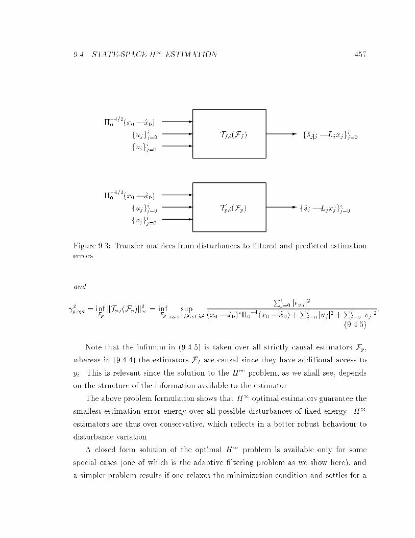
���� STATE�SPACE H� ESTIMATION �
�
�
�
�
�
�
�
� � f�sj � Ljxjgij��
f�sjjj � Ljxjgij��
Tp�i�Fp�
Tf�i�Ff�fujgij��
fvjgij��
fujgij��
������ �x� � �x��
fvjgij��
������ �x� � �x��
Figure ���� Transfer matrices from disturbances to �ltered and predicted estimationerrors�
and
��p�opt � infFp
kTp�i�Fp�k�� � inf
Fp
supx��u�h��v�h�
Pij�� jep�ij
�
�x� � �x��������x� � �x�� �
Pij�� jujj
� �Pi
j�� jvjj��
������
Note that the in�mum in ������ is taken over all strictly causal estimators Fp�
whereas in ����� the estimators Ff are causal since they have additional access to
yi� This is relevant since the solution to the H� problem� as we shall see� depends
on the structure of the information available to the estimator�
The above problem formulation shows that H� optimal estimators guarantee the
smallest estimation error energy over all possible disturbances of �xed energy� H�
estimators are thus over conservative� which re�ects in a better robust behaviour to
disturbance variation�
A closed form solution of the optimal H� problem is available only for some
special cases �one of which is the adaptive �ltering problem as we show here�� and
a simpler problem results if one relaxes the minimization condition and settles for a

�� CHAPTER �� H� OPTIMALITY OF THE LMS ALGORITHM
suboptimal solution�
Problem ��� �Sub�optimal H� Problem� Given scalars �f � � and �p � ��
�nd estimation strategies �siji � Ff�y�� y�� � � � � yi� and �si � Fp�y�� y�� � � � � yi��� that
respectively achieve k Tf�i�Ff� k�� �f and k Tp�i�Fp� k�� �p� This clearly requires
checking whether �f � �f�o and �p � �p�o�
The above two problem formulations are for the �nite horizon case� In the in�nite
horizon case� to guarantee that kTf �F�k� � �f and kTp�F�k� � �p we need to ensure
kTf�i�F�k� � �f and kTp�i�F�k� � �p for all i�
����� The H� Filters
We now brie�y review the solutions of the H� �ltering problems using the notation
of �HSK��c� HSK��b��
Theorem ���� �The H� A Posteriori Filter� For a given � � �� if the Fi are
nonsingular then an estimator with kTf�ik� � � exists if� and only if�
P��j �H�
jHj � ���L�jLj � �� j � �� � � � � i ������
where P� � ��� and Pj satis�es the Riccati recursion
Pj�� � FjPjF�j �GjG
�j �
hL�j H�
j
iR��
e�j
�� Lj
Hj
��PjF
�j �����
with
Re�j �
�� ���I �
� I
���
�� Lj
Hj
��Pj
hL�j H�
j
i�
If this is the case� then one possible H� �lter with level � is given by
�sjjj � Lj�xjjj�
where �xjjj is recursively computed as
�xj��jj�� � Fj�xjjj �Kf�j���yj�� �Hj��Fj�xjjj�� �x��j�� � initial guess ������

���� STATE�SPACE H� ESTIMATION ��
and
Kf�j�� � Pj��H�j���I �Hj��Pj��H
�j���
��� ������
Theorem ��� �The H� A Priori Filter� For a given � � �� if the Fi are non�
singular then an estimator with kTp�ik� � � exists if� and only if�
P��j � P��
j � ���L�jLj � �� j � �� � � � � i ���� ��
where Pj is the same as in Theorem ����� If this is the case� then one possible H�
�lter with level � is given by
�sj � Lj�xj� ���� �
�xj�� � Fj�xj �Kp�j�yj �Hj �xj�� �x� � initial guess ���� ��
where
Kp�j � Fj PjH
�j �I �Hj
PjH�j ���� ���� ��
Note that the above two estimators bear a striking resemblance to the celebrated
Kalman �lter���� �xj�� � Fj�xj � FjPjH
�j �I �HjPjH
�j ����yj �Hj �xj�
Pj�� � FjPjF�j �GjG
�j � FjPj�I �HjPjH
�j ���PjF
�j
���� �
and that the only di�erence is that the Pj of equation ������� and Pj of equation
���� ��� satisfy Riccati recursions that di�er with that of ���� �� However� as
� �� the Riccati recursion ����� collapses to the Kalman �lter recursion ���� ��
This suggests that the H� norm of the Kalman �lter may be quite large� indicating
that it may have poor robustness properties�
It is also interesting that the structure of the H� estimators depends� via the
Riccati recursion ������ on the linear combination of the states that we intend to
estimate �i�e�� the Li�� This is as opposed to the Kalman �lter� where the estimate
of any linear combination of the state is given by that linear combination of the state

�� CHAPTER �� H� OPTIMALITY OF THE LMS ALGORITHM
estimate� Intuitively� this means that the H� �lters are speci�cally tuned towards
the linear combination Lixi�
Note also that condition ���� �� is more stringent than condition ������� indi�
cating that the existence of an a priori �lter of level � implies the existence of an a
posteriori �lter of level �� but not necessarily vice versa�
We further remark that the �lter of Theorem ��� �and Theorem ����� is one of
many possible �lters with level �� A full parametrization of all estimators of level �
are given by the following Theorems� �For proofs see �HSK��b� or Chapter ���
Theorem ���� �All H� A Posteriori Estimators� All H� a posteriori estima�
tors that achieve a level �f assuming they exist� are given by
�sjjj � Lj �xjjj � ���fI � Lj�P��j �H�
jHj���L�j �
�
� ���� ��
Sj�I �HjPjH
�j �
�
� �yj �Hj �xjjj�� � � � � �I �H�P�H�� �
�
� �y� �H��x�j��
where �xjjj satis�es the recursion
�xj��jj�� � Fj�xjjj �Kf�j���yj�� �Hj��Fj�xjjj��Kc�j��sjjj � Lj �xjjj� ���� ��
with Kf�j�� the same as in Theorem �����
Kc�j � �I � Pj��Hj��H�j���
��Fj�P��j �HjH
�j � ���f LjL
�j ���L�j � ���� �
and
S�aj� � � � � a�� �
���������
S��a��
S��a�� a�����
Sj�aj� � � � � a��
���������
is any possibly nonlinear� contractive causal mapping� i�e��
kXj��
jSj�aj� � � � � a��j� �
kXj��
jajj� for all k � �� � � � � � i�

��� MAIN RESULT �
Theorem ��� �All H� A Priori Estimators� All H� a priori estimators that
achieve a level �p assuming they exist� are given by
�sj � Lj �xj � ���pI � LjPjL�j �
�
� ���� ��
Sj�I �Hj��
Pj��H�j���
� �
� �yj�� �Hj��!xj���� � � � � �I �H� P�H
�� �� �
� �y� �H�!x��
where
!xk � �xk � PkL�k���
�pI � LkPkL
�k�����sk � Lk�xk�� ���� ��
�xj satis�es the recursion
�xj��jj � Fj�xjjj�� � FjPj
hL�j H�
j
iR��
e�j
�� �sj � Lj�xjjj��
yj �Hj �xjjj��
�� � �������
with Pj � Pj and Re�j given by Theorem ������ and S is any possibly nonlinear� con�
tractive causal mapping�
Note that although the �lters obtained in Theorems ��� and ���� are linear�
the full parametrization of all H� �lters with level � is given by a nonlinear causal
contractive mapping S� The �lters of Theorems ��� and ���� are known as the
central �lters and correspond to S � �� These central �lters have a number of other
interesting properties� They correspond� as we shall see in a subsequent section� to the
risk�sensitive optimal �lter �Whi���� and can be shown to be the maximum entropy
�lter �GM���� �See also Sec� � and Sec� ����
��� Main Result
Let us �rst note that the basic equation of the adaptive �ltering model ����� � can be
rewritten in the following state�space form���� xi�� � xi
di � hixi � vix� � w� ����� �
This is a relevant step since it reduces the adaptive �ltering problem to an equivalent
state�space estimation problem� This point of view has been recently proposed in

�� CHAPTER �� H� OPTIMALITY OF THE LMS ALGORITHM
�SK�b� where a uni�ed square�root�based derivation of exponentially�weighted RLS
adaptive algorithms is obtained by reformulating the original adaptive problem as a
state�space linear least�squares estimation problem and then applying various algo�
rithms from Kalman �lter theory� Here we shall instead apply the H� theory to the
state�space model ����� � and show that the optimum a priori and a posteriori H�
�lters reduce to the LMS and normalized LMS algorithms� respectively�
At this point we need one more de�nition�
De�nition �� �� �Exciting Inputs� The input vectors hi are called exciting if� and
only if�
limN��
NXi��
hih�i � �
����� The Normalized LMS Algorithm
We �rst consider the a posteriori �lter and show that it collapses to the normalized
LMS algorithm�
Theorem �� �� �Normalized LMS Algorithm� Consider the state�space model
�� ��� and suppose we want to minimize the H� norm of the transfer operator
Tf �F� from the unknowns ������w � �wj��� and fvjg�j�� to the �ltered error fef�j �
�sjjj � hjwg�j��� If the input data fhjg is exciting� then the minimum H� norm is
�f�opt � �
In this case� the central optimal H� a posteriori �lter is
�sjjj � hj �wjj�
where �wjj is given by the normalized LMS algorithm with parameter ��
�wjj�� � �wjj ��h�j��
� �hj��h�j���dj�� � hj�� �wjj�� �wj�� � initial guess� �������

��� MAIN RESULT ��
Intuitively it is not hard to convince oneself that �f�opt cannot be less than one�
To this end� suppose that the estimator has chosen some initial guess �wj��� Then
one may conceive of a disturbance that yields an observation that coincides with the
output expected from �wj��� i�e� �
hi �wj�� � hiw � vi � di�
In this case one expects that the estimator will not change its estimate of w� so that
�wji � �wj�� for all i� Thus the �ltered error is
ef�i � hiw � hi �wji � hiw � hi �wj�� � �vi�
and the ratio in ������� becomes
kvk�
���jw � �wj��j� � kvk��
khi�w � �wj���k�
���jw � �wj��j� � khi�w � �wj���k��
When the fhig are exciting� for any � � �� we can �nd a weight vector w and an
integer N such thatPN
i�� jhi�w � �wj���j� �
jw� �wj��j�
��� With these choices we have
PNi�� jhi�w � �wj���j
�
���jw � �wj��j� �PN
i�� jhi�w � �wj���j�� � ��
so that the ratio in ������� can be made arbitrarily close to one�
The surprising fact though is that �f�opt is exactly one and that the normalized
LMS algorithm achieves it� What this means is that normalized LMS guarantees that
the energy of the �ltered error will never exceed the energy of the disturbances� This
is not true for other estimators� For example� in the case of the recursive least�squares
�RLS� algorithm� one can come up with a disturbance of small energy that will yield
a �ltered error of large energy �see �HK�b� and Chapter ���
Proof of Theorem �� ��� We apply the a posteriori �lter of Theorem ��� to the
state�space model ����� � where Fi � I� Gi � �� Hi � hi� and Li � hi� Thus the
Riccati equation simpli�es to
Pi�� � Pi � Pi
hh�i h�i
i����� ���I �
� I
���
�� hj
hj
��Pi
hh�i h�i
i ���� �� hi
hi
��Pi�

� CHAPTER �� H� OPTIMALITY OF THE LMS ALGORITHM
which� using the matrix inversion lemma �Kai���� implies that
P��i�� � P��
i �hh�i h�i
i �� ����I �
� I
���� hi
hi
��
� P��i � � � ����h�ihi�
Consequently� starting with P��� � ���I� we get
P��i�� � ���I � � � ����
iXj��
h�jhj � �������
Now we need to check the existence condition ������ and �nd the optimum �f�opt� It
follows from the above expression for P��i�� that we have
P��i�� �H�
i��Hi�� � ���L�i��Li�� � ���I � � � ����i��Xj��
h�jhj� ������
Suppose � � so that � ��� � �� Since the fhjg are exciting� we conclude that for
some k� and for large enough i� we must have
i��Xj��
jhjkj� �
���
��� � �
This implies that the kth diagonal entry of the matrix on the right hand side of ������
is negative� viz��
��� � � � ����i��Xj��
jhjkj� � ��
Consequently� P��i���H�
i��Hi��� ���L�i��Li�� cannot be positive�de�nite� Therefore�
�f�opt � � We now verify that �f�opt is indeed � For this purpose� we note that if
we consider � � then from equation ������� we have Pi � �I � � for all i and the
existence condition is satis�ed� If we now write the a posteriori �lter for �f�opt � �
with Pi � �I� we get the desired so�called normalized LMS algorithm ��������
����� The LMS Algorithm
We now apply the a priori H���lter and show that it collapses to the LMS algorithm�

��� MAIN RESULT ��
Theorem �� � �LMS Algorithm� Consider the state�space model �� ��� and
suppose we want to minimize the H� norm of the transfer operator Tp�F� from the
unknowns ������w� �wj��� and fvjg�j�� to the predicted error fep�j � �sj �hjwg�j��� If
the input data fhjg is exciting� and
� � � � infi
hih�i�������
then the minimum H� norm is
�p�opt � �
In this case� the central optimal a priori H� �lter is
�sj � hi �wjj��
where �wjj�� is given by the LMS algorithm with learning rate �� viz��
�wjj � �wjj�� � �h�j �dj � hj �wjj��� � �wj��� �������
Proof� The proof is similar to that for the normalized LMS case� For � � � the
matrix Pi of Theorem ���� cannot be positive�de�nite� For � � � we get Pi � �I � �
for all i� and
P��i � P��
i � L�iLi
� ���I � h�ihi
It is straightforward to see that the eigenvalues of P��i are
f���� ���� ���� ���� ��� � hih�i g�
Thus P��i is positive de�nite if� and only if� ������� is satis�ed� which leads to �p�opt �
� Writing the H� a priori �lter equations for � � yields
�wji � �wji�� � Pih�i �I � hi Pih
�i ����di � hi �wji���
� �wji�� � Pi�I � h�ihi Pi�
��h�i �di � hi �wji���
� �wji�� � � P��i � h�ihi�
��h�i �di � hi �wji���
� �wji�� � �h�i �di � hi �wji����

�� CHAPTER �� H� OPTIMALITY OF THE LMS ALGORITHM
The above result indicates that if the learning rate � is chosen according to ��������
then LMS ensures that the energy of the predicted error will never exceed the energy
of the disturbances� It is interesting that we have obtained an upper bound on the
learning rate � that guarantees this H� optimality� since it is a well known fact that
LMS behaves poorly if the learning rate is chosen too large� It is also interesting to
compare the bound in ������� with the bounds studied in �WS��� and �Wid���
We further note that if the input data is not exciting� thenP�
i�� h�ihi will have a
�nite limit� and the minimumH� norm of the a posteriori and a priori �lters will be
the smallest � that ensures
���I � � � �����Xi��
h�ihi � ��
This will in general yield �opt � � and Theorems ��� and ���� can be used to write
the optimal �lters for this �opt� In this case the LMS and normalized LMS algorithms
will still correspond to � � � but will now be suboptimal�
�� An Illustrative Example
To illustrate the robustness of the LMS algorithm we consider a special case of model
����� �� where hi is now a scalar that randomly takes on the values � and � �
Using the LMS algorithm we can write the following state�space model for the
predicted error ep�i � hixi � hi�xi���� xi�� � � � �jhij�� xi � �h�i vi � � � �� xi � �hivi
ep�i � hi xi� x� � w � �x�� ����� �
where xi � xi� �xi� and where we have used the fact that the hi have magnitude one�
Assuming we have observed N points of data� we can then use ����� � to write the
operator� Tlms�N ���� that maps the disturbances f���
� x�� fvigN��i�� g to the fep�ig
N��i�� ��
������ep��
ep�����
ep�N��
�������

��� AN ILLUSTRATIVE EXAMPLE �
���������
��
� h� � � � � � �
��
� �� ��h� ��h�h� � � � � �
��
� �� ���h� �� � � ��h�h� ��h�h� � � � ����
������
� � ����
��
� �� ��N��hN�� �� �� ��N��hN��h� �� �� ��N��hN��h� � � � ��hN��hN��
���������
� �z �Tlms�N ���
�������
���
� �x�
v����
vN��
������� �
������
Suppose now we use the RLS algorithm �viz� the Kalman �lter� to estimate the
states in ����� �� i�e��
�xi�� � �xi � kp�i�di � hi�xi�
where kp�i �pih
�i
��pijhij�and
pi�� � pi �jhij�p�i
� pijhij�� pi �
p�i � pi
�pi
� pi� p� � �� �������
Then we may write the following state�space model for the RLS predicted error e�
p�i �
hixi � hi�xi� ��� xi�� � � � kp�ihi� xi � kp�ivi
e�
p�i � hi xi� x� � w � �x�� ������
Now solving ������� yields
pi ��
� i�� �������
and
kp�i � hipi��� � kp�ihi �pi��pi
� �������
Using �������� �������� and the state�space model ������ we can also write the
transfer operator Trls�N ��� that maps the disturbances to the predicted errors as
follows�
�������
e�
p��
e�
p��
���
e�
p�N��
�������
���������
��
�h� � � � � � �
��
�h����
��h�h����
� � � � �
��
�h�
���� �� h�h����� �� h�h�
���� � � � ����
������
� � ����
��
�hN��
���N���� ��hN��h�
���N���� ��hN��h�
���N���� � � � ��hN��hN��
���N����
���������
� �z �Trls�N���
�������
���
�x�
v����
vN��
������� �
������
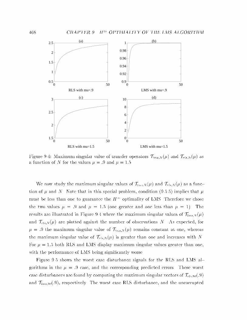
�� CHAPTER �� H� OPTIMALITY OF THE LMS ALGORITHM
0.5
1
1.5
2
2.5
0 50
(a)
RLS with mu=.9
0.9
0.92
0.94
0.96
0.98
1
0 50
(b)
LMS with mu=.9
1.5
2
2.5
3
0 50
(c)
RLS with mu=1.5
0
2
4
6
8
10
0 50
(d)
LMS with mu=1.5
Figure ��� Maximum singular value of transfer operators Tlms�N ��� and Trls�N��� asa function of N for the values � � �� and � � ���
We now study the maximum singular values of Tlms�N ��� and Trls�N ��� as a func�
tion of � and N � Note that in this special problem� condition ������� implies that �
must be less than one to guarantee the H� optimality of LMS� Therefore we chose
the two values � � �� and � � �� �one greater and one less than � � �� The
results are illustrated in Figure �� where the maximum singular values of Tlms�N ���
and Trls�N��� are plotted against the number of observations N � As expected� for
� � �� the maximum singular value of Tlms�N ��� remains constant at one� whereas
the maximum singular value of Trls�N��� is greater than one and increases with N �
For � � �� both RLS and LMS display maximum singular values greater than one�
with the performance of LMS being signi�cantly worse�
Figure ��� shows the worst case disturbance signals for the RLS and LMS al�
gorithms in the � � �� case� and the corresponding predicted errors� These worst
case disturbances are found by computing the maximum singular vectors of Trls�������
and Tlms�������� respectively� The worst case RLS disturbance� and the uncorrupted

��� AN ILLUSTRATIVE EXAMPLE ��
-1
-0.5
0
0.5
1
0 50
(a)
-1
-0.5
0
0.5
0 50o
o
ooo
o
oo
oo
oo
oooo
ooooooooooo
ooooooooooooooooooooooo
(b)
-1
-0.5
0
0.5
1
0 50
(c)
-1
-0.5
0
0.5
1
0 50oo
ooo
o
oo
oo
oo
oooo
ooooo
o
o
o
ooo
oo
o
o
ooo
oo
oooo
o
oo
oo
o
oooo
(d)
Figure ���� Worst case disturbances and the corresponding predicted errors for RLSand LMS� �a� The solid line represents the uncorrupted output hixi and the dashedline represents the worst case RLS disturbance� �b� The dashed line and the dottedline represent the RLS and LMS predicted errors� respectively� for the worst caseRLS disturbance� �c� The solid line represents the uncorrupted output hixi and thedashed line represents the worst case LMS disturbance� �d� The dashed line and thedotted line represent the RLS and LMS predicted errors� respectively� for the worstcase LMS disturbance�
output hixi� are depicted in Figure ���a� As can be seen from Figure ���b� the corre�
sponding RLS predicted error does not go to zero �it is actually biased�� whereas the
LMS predicted error does� The worst case LMS disturbance signal is given in Figure
���c� and as before� the LMS predicted error tends to zero� while the RLS predicted
error does not� The form of the worst case disturbances �especially for RLS� are quite
interesting� they compete with the true output early on� and then go to zero�
The disturbance signals considered in this example are rather contrived and may
not happen in practice� However� they serve to illustrate the fact that the RLS
algorithm may have poor performance even if the disturbance signals have small
energy� On the other hand� LMS will have robust performance over a wide range of
� CHAPTER �� H� OPTIMALITY OF THE LMS ALGORITHM
disturbance signals�
���� Discussion
In Sec� ���� we motivated the �f�opt � result for normalized LMS by considering
a disturbance strategy that made the observed output di coincide with the expected
output hi �wj��� It is now illuminating to consider the dual strategy for the estimator�
Recall that in the a posteriori adaptive �ltering problem the estimator has access
to observations d�� d�� � � � � di and is required to construct an estimate of �siji of the
uncorrupted output si � hixi� The dual to the above mentioned disturbance strategy
would be to construct an estimate that coincides with the observed output� viz��
�siji � di� �������
The corresponding �ltered error is�
ef�i � �siji � hixi � di � hixi � vi�
Thus the ratio in ������� can be made arbitrarily close to one� and the estimator
������� will achieve the same �f�opt � that the normalized LMS algorithm does�
The fact that the simplistic estimator ������� �which is obviously of no practical
use� is an optimal H� a posteriori �lter seems to question the very merit of being
H� optimal� A �rst indication towards this direction may be the fact that the H�
estimators that achieve a certain level � are nonunique� In our opinion� the property
of beingH� optimal �i�e� � of minimizing the energy gain from the disturbances to the
errors� is a desirable property in itself� The high sensitivity of the RLS algorithm to
di�erent disturbance signals� as illustrated in the example of Sec� ���� clearly indicates
the desirability of the H� optimality property� However� di�erent estimators in the
set of allH� optimal estimators may have drastically di�erent behaviour with respect
to other desirable performance measures�
In Sec� �� we develop the full parametrization of all H� optimal a posteriori
and a priori adaptive �lters� and show how to obtain ������� as a special case of
this parametrization� Moreover� it can be shown �see �HHK���� that among all H��
optimal a posteriori �lters the �lter ������� has the worst H� �or� roughly speaking�

���� ALL H� ADAPTIVE FILTERS
average� performance� Thus it is the least desirable H��optimal �lter with respect
to an H� criterion� On the other hand� as indicated in Theorems ���� and ������
the LMS and normalized LMS algorithms correspond to the so�called central �lters�
These central �lters have other desirable properties that we discuss in Sec� ���� they
are risk�sensitive optimal and can also be shown to be maximum entropy�
The main problem with the estimator ������� is that it makes absolutely no use
of the state�space model ����� �� We should note that it is not possible to come up
with such a simple minded estimator in the a priori case� indeed as we shall see in
the next section� the a priori estimator corresponding to ������� is highly nontrivial�
The reason seems to be that since in the a priori case one deals with predicted error
energy� it is inevitable that one must make use of the state�space model ����� � in
order to construct an optimal prediction of the next output� Thus in the a priori case�
the problems arising from such unreasonable estimators such as ������� are avoided�
�� All H� Adaptive Filters
In Sec� ���� we came up with an alternative optimal H� a posteriori �lter� We now
use the results of Theorems ���� and ��� to parametrize all optimal H� a priori
and a posteriori �lters�
Theorem ����� �All H� A Posteriori Adaptive Filters� If the input date fhig
is exciting� all H� optimal a posteriori adaptive �lters that achieve �f�opt � are
given by
�sjjj � hj �wjj�� ��hjh�j �� �
�Sj� � �hjh
�j �
�
� �dj � hj �wjj�� � � � � � � �h�h���
�
� �d� � h� �wj��
���� �
where �wjj satis�es the recursion
�wjj�� � �wj ��h�j��
� �hj��h�j���dj�� � hj�� �wjj��
�h�j � �hj��h�j��
��sjjj � hj �wjj�� �wj��
������
and S is any possibly nonlinear� contractive causal mapping�
� CHAPTER �� H� OPTIMALITY OF THE LMS ALGORITHM
Proof� Simply restating the result of Theorem ���� for the special case Fj � I�
Gj � �� Hj � hj and Lj � hj � and using the identity
I � hj�P��j � h�jhj�
��h�j � �I � hjPjh�j ����
along with the fact that for the H��optimal a posteriori adaptive �lters we have
�f�opt � and Pi � �I� yields the desired result�
We can now note the signi�cance of some special choices for the causal contraction
S�
�i� S � � � This yields the normalized LMS algorithm�
�ii� S � I � This yields
�sjjj � hj �wjj � � � �hjh�j �� �
� � � �hjh�j�
�
� �dj � hj �wjj� � dj �
which is the simple minded estimator of Sec� ���� �
�iii� S � �I � This yields
�sjjj � hj �wjj � � � �hjh�j �� �
� � � �hjh�j �
�
� �dj � hj �wjj� � �hj �wjj � dj�
so that the recursion for �wjj becomes
�wjj�� � �wj��h�j��
� �hj��h�j���dj���hj�� �wjj��
�h�j � �hj��h�j��
�dj�hj �wjj�� �wj���
Theorem ���� �All H� A Priori Adaptive Filters� If the input data fhig is
exciting� and � � � � infi�
hih�i� then all H� optimal a priori adaptive �lters are given
by
�sj hj �wjj��� ���hjh�j �
�
�Sj
�� �hj��h
�j���
�
� dj�� � hj�� �wjj���� � � � � �� �h�h���
�
� d� � h� �wj����
������
where
!wjk�� � �wjk�� ��h�k
� � �hkh�k��sk � hk �wjk���� �����
�wjj satis�es the recursion
�wjj � �wjj�� � �h�j �dj � hj �wjj���� �h�j ��sj � hj �wjj���� �wj�� ������
and S is any possibly nonlinear� contractive causal mapping�

���� RISK�SENSITIVE OPTIMALITY �
Proof� Simply restating the result of Theorem ��� for the special case Fj � I�
Gj � �� Hj � hj and Lj � hj � and using the fact that for the H��optimal a priori
�lter we have �p�opt � � Pi � �I and Pi � �I � h�ihi� yields the desired result�
Indeed equations ������� ����� and ������ are the corresponding specializations of
equations ���� ��� ���� �� and �������� respectively�
We once more note the consequences of some special choices of the causal con�
traction S�
�i� S � � � This yields the LMS algorithm�
�ii� S � I � This yields
�sj � hj �wjj�� � � � �hjh�j �
�
� � � �hj��h�j���
�
� �dj�� � hj�� !wjj����
where !wjj�� and �wjj�� satisfy ����� and ������� The above �lter is the a priori
adaptive �lter that corresponds to the simple minded estimator of Sec� ���� �
Note that in this case the �lter is highly nontrivial�
�iii� S � �I � This yields
�sj � hj �wjj�� � � � �hjh�j �
�
� � � �hj��h�j���
�
� �dj�� � hj�� !wjj����
Note that it does not seem possible to obtain a simplistic a priori estimator that
achieves optimal performance�
��� Risk�Sensitive Optimality
In this section we focus on a certain property of the central H� �lters� namely the
fact that they are risk�sensitive optimal �lters� This will give further insight into
the LMS and normalized LMS algorithms� and in particular will provide a stochas�
tic interpretation in the special case of disturbances that are independent Gaussian
random variables�

CHAPTER �� H� OPTIMALITY OF THE LMS ALGORITHM
The risk�sensitive �or exponential cost� criterion was introduced in �Jac�� and
further studied in �SDJ� Whi��� SFB���� We begin with a brief introduction to the
risk�sensitive criterion� For much more on this subject consult �Whi����
���� The Exponential Cost Function
Although it is straightforward to consider the risk�sensitive criterion in the full gen�
erality of the state�space model of Sec� ��� here we only deal with the special case
of our interest� To this end� consider the state�space model corresponding to the
adaptive �ltering problem we have been studying�
��� xi�� � xi
di � hixi � vi� x� � w ����� �
where we now assume that w and the fvig are independent Gaussian random variables
with means �wj�� and zero and covariances �� and I� respectively� As before� we
are interested in the �ltered and predicted estimates �siji � Ff�d�� d�� � � � � di� and
�si � Fp�d�� d�� � � � � di��� of the uncorrupted output si � hixi� The corresponding
�ltered and predicted errors are given by ef�i � �siji � si and ep�i � �si � si� The
conventional Kalman �lter is an estimator that performs the following minimization
�see e�g� �Jaz�� AM����
minf�sjg
��E iX
j��
e�p�jep�j
�� � �������
where the expectation is taken over the Gaussian random variables w and fvjg�j��
whose joint conditional distribution is given by�
p�w� v�� � � � � vijd�� � � � � di�
exp
���
�
���w � �wj���
����� �w � �wj��� �
iXj��
�dj � hjxj���dj � hjxj�
�A�� �
and where the symbol stands for "proportional to"� In the terminology of �Whi����
the �lter that minimizes ������� is known as the risk�neutral �lter�
�In fact� this is done in Sec� ����

���� RISK�SENSITIVE OPTIMALITY �
An alternative criterion that is risk�sensitive has been extensively studied in
�Jac�� Whi��� SFB��� and corresponds to the following minimization problem
minf�sjjjg
�f�i�� � minf�sjjjg
���
log
�Eexp��
�Cf�i�
��� �������
or
minf�sjg
�p�i�� � minf�sjg
���
log
�Eexp��
�Cp�i�
��� ������
where Cf�i �Pi
j�� e�f�ief�i and Cp�i �
Pij�� e
�p�iep�i� The criteria in ������� and ������
are known as the a posteriori and a priori exponential cost functions� and any �lters
that minimize �f�i�� and �p�i�� are referred to as a posteriori and a priori risk�
sensitive �lters� respectively� The scalar parameter is correspondingly called the
risk�sensitivity parameter� Some intuition concerning the nature of this modi�ed
criterion is obtained by expanding �i�� �where we have dropped the subscripts f
and p since the argument follows for both �ltered and predicted estimates� in terms
of and writing�
�i�� � E�Ci��
Var�Ci� �O����
The above equation shows that for � �� we have the risk�neutral case �i�e�� the
conventional Kalman �lter�� When � �� we seek to maximize Eexp�� ��Ci�� which
is convex and decreasing in Ci� Such a criterion is termed risk�seeking �or optimistic�
since larger weights are on small values of Ci� and hence we are more concerned with
the frequent occurrence of moderate values ofCi than with the occasional large values�
When � �� we seek to minimize Eexp�� ��Ci�� which is convex and increasing in
Ci� Such a criterion is termed risk�averse �or pessimistic� since large weights are on
large values of Ci� and hence we are more concerned with the occasional occurrence
of large values than with the frequent occurrence of moderate ones�
The relationship between the risk�sensitive criterion and the H� criterion was
�rst noted in �GD��� and has been further discussed in �Whi��� HSK��b�� It may be
formally stated as follows� In the risk�averse case � �� the risk�sensitive optimal
�lter with parameter is given by the central H� �lter with level � � ���
� � In
particular� there is a certain smallest value of the risk�sensitivity parameter !� after
which the minimizing property of �i�� breaks down� and it is this value that yields
the optimal central H� �lter with �opt � �!�����
� CHAPTER �� H� OPTIMALITY OF THE LMS ALGORITHM
���� Risk�sensitive Adaptive Filtering
Using the discussion of Sec� ���� � we are now in a position to state the risk�sensitive
results for LMS and normalized LMS�
Theorem ����� �Normalized LMS and Risk�sensitivity� Consider the state�space
model ����� where the w and fvjg are independent Gaussian random variables with
means �wj�� and �� and variances �I and I� respectively� The solution to the following
minimization problem
minf�sjjjg
�f �� � minf�sjjjg
��log
�Eexp�
�Cf ��
���������
where Cf �P�
j�� e�f�ief�i� and the expectation is taken over w and fvjg subject to
observing fd�� d�� � � � � dig� is given by the normalized LMS algorithm
�siji � hi �wji�
and
�wji�� � �wji ��h�i��
� �hi��h�i���di�� � hi�� �wji� � �wj��� �������
Theorem ���� �LMS and Risk�sensitivity� Consider the state�space model �����
where the w and fvjg are independent Gaussian random variables with means �wj��
and �� and variances �I and I� respectively� Suppose moreover� that the fhig are
exciting� and that
� � � � infi
hih�i�
Then the solution to the following minimization problem
minf�sjg
�p�� � minf�sjg
��log
�Eexp�
�Cp��
��������
where Cp �P�
j�� e�p�iep�i� and the expectation is taken over w and fvjg subject to
observing fd�� d�� � � � � di��g� is given by the LMS algorithm
�si � hi �wi���

���� FURTHER REMARKS
0 0.5 1 1.5 2 2.5 30
0.5
1
1.5
2
2.5
3
3.5
Cp
exp(
Cp/
2)−
1
Figure ���� The criterion ������ is termed risk averse �or pessimistic� since the costfunction exp�Cp�� is very large for large values of Cp� Hence we are more concernedwith the occasional occurrence of large values of Cp than with the frequent occurrenceof moderate ones� This fact corresponds well with the intuition gained from the H�
optimality of the LMS algorithm� We have also plotted Cp� �the dashed line� tocompare the two cost functions� since the RLS algorithm minimizes the expectedvalue of Cp��
and
�wji � �wji�� � �h�i �di � hi �wji��� � �wj��� �������
Before closing this section we should remark that the central H� �lters possess
other properties in addition to the one described above� In the game theoretic for�
mulation of H� estimation� the central �lter corresponds to the solution of the game
�see e�g�� �BB��� and Sec� ���� Moreover� among all H� estimators that achieve a
certain level �� the central solution can be shown to be the maximum entropy �GM���
solution� However� we shall not pursue these directions here�
��� Further Remarks
In addition to yielding a new interpretation for the LMS algorithm and providing it
with a rigorous basis� the results described in this chapter have lent themselves to
various generalizations and have allowed the authors to obtain several new results�
� CHAPTER �� H� OPTIMALITY OF THE LMS ALGORITHM
We close this chapter by listing some of these ideas and results here� We should also
mention that we believe the framework presented in this chapter provides a new way
of looking at adaptive algorithms and should be worthy of further scrutiny�
LMS with Time�Varying Learning Rate
In many applications one uses the LMS algorithm with time�varying stepsize �or
learning rate�� viz��
�wji � �wji�� � �ih�i �di � hi �wji���� �wj��� ����� �
In this case� it is straightforward to show that if the vectors f����i hig are exciting�
and if �ihih�i � for all i� then the LMS algorithm with time�varying stepsize solves
the following minimax problem�
infF
supw�v�h�
P�j�� �jjep�jj
�
jw � �wj��j� �P�
j�� �j jvjj�� � �������
H� Adaptive Filtering
In this chapter we have shown that if adaptive �ltering for output prediction error is
considered then the central H��optimal adaptive �lter is LMS� It is also possible to
consider prediction of the �lter weight vector itself� and for the purpose of coping with
time�variations� to consider exponentially weighted� �nite�memory and time�varying
adaptive �ltering� This results in some new adaptive �ltering algorithms that may be
useful in uncertain and non�stationary environments �see �HK�a� and Chapter ��
H� Norm Bounds for the RLS Algorithm
In order to compare the robustness of H��optimal algorithms �such as RLS� withH��
optimal algorithms �such as LMS� it it useful to obtain H� norm bounds for these
algorithms� This has been done for the RLS algorithm in �HK�b� �see also Chapter
��� where it is shown that unlike LMS� the H� norm of the RLS algorithm depends
on the input data fhig and� roughly speaking� grows linearly in the parameter ��

��� � CONCLUSION �
A Time�Domain Feedback Analysis
Using some of the ideas presented here� a time�domain feedback analysis of recursive
adaptive schemes� including gradient�based and Gauss�Newton �lters has been devel�
oped �SR��a� SR��b�� for both the FIR and IIR contexts� The analysis highlights
an intrinsic feedback structure in terms of a feedforward lossless or contractive map
and a feedback memoryless or dynamic map� The structure lends itself to analysis
via energy conservation arguments and via standard tools in system theory such as
the small gain theorem �Kha��� Vid���� It further suggests choices for the adaptation
gains �or step�sizes� in order to enforce a robust performance in the presence of dis�
turbances �along the lines of H�theory�� as well as improve the convergence speed of
the adaptive algorithms�
Nonlinear Problems
The results presented in this chapter are for linear adaptive �lters and can be some�
what generalized to nonlinear adaptive �lters �such as neural networks� if one lin�
earizes these nonlinear models around some suitable point� Using this approach it
can be shown �see �HSK�a�� that� for nonlinear problems� instantaneous�gradient�
based algorithms �such as backpropagation �RM���� are locally H��optimal� This
means that if the initial estimate of the weight vector is close enough to its true
value� and if the disturbances are small enough� then the maximum energy gain from
the disturbances to the output prediction errors is arbitrarily close to one� Global
H��optimal �lters can also be found in the nonlinear case� but they have the draw�
back of being in�nite�dimensional �see �HK��b���
���� Conclusion
We have demonstrated that the LMS algorithm is H� optimal� This result solves
a long standing issue of �nding a rigorous basis for the LMS algorithm� and also
con�rms its robustness� We �nd it quite interesting that despite the fact that there
has only been recent interest in the �eld of H� estimation� there has existed an H�

�� CHAPTER �� H� OPTIMALITY OF THE LMS ALGORITHM
optimal estimation algorithm that has been widely used in practice for the past three
decades�

��A� A FIRST PRINCIPLES PROOF OF THE H� OPTIMALITY OF LMS �
��A A First Principles Proof of the H� Optimality
of LMS
In this appendix we shall outline a �rst principles proof of the H� optimality of the
LMS and normalized LMS algorithms that does not require the results of Theorems
��� and ���� on H� �ltering� The proofs rely on some easily veri�ed inequalities�
We begin with normalized LMS� �See also the last section in �SK�b� and �SR��a���
��A�� The Normalized LMS Algorithm
Recall that in Sec� ���� � after the statement of Theorem ���� � we constructed a
disturbance signal such that for any � � ��
kefk�
���jw � �wj��j� � kvk�� � ��
Since this was just one special disturbance signal� we conclude that if the input vectors
are exciting� we have
supw�v�h�
kefk�
���jw � �wj��j� � kvk�� � ���A� �
We shall now show that the normalized LMS algorithm achieves one in the above
inequality� This� of course� also shows that �f�opt � � To this end� note that the
normalized LMS algorithm
�wjj � �wjj�� �h�j
��� � hjh�j�dj � hj �wjj����
can� after some rearrangement� be written as
�wjj�� � �wjj � �h�i �dj � hj �wjj��
If we now de�ne wjj � w � �wjj� the above expression allows us to write
�����h wjj��
i� �����
h wjj � �h�i �dj � hj �wjj�
i� ���A���

�� CHAPTER �� H� OPTIMALITY OF THE LMS ALGORITHM
�The reason for multiplying both sides by ����� will become clear in a moment�� On
the other hand� we may write vj � dj � hjw as
vj � �dj � hj �wjj�� hj wjj� ���A���
Squaring both sides of ���A��� and ���A��� and adding the results yields
���j wjj��j� � jvjj
� � ���j wjjj� � jhj wjjj
� � � � �hjh�j ��dj � hj �wjj�
�� ���A��
Now since the third term on the RHS of the above expression is positive� and since
hj wjj � ef�j� we may write
���j wjj��j� � jvjj
� � ���j wjjj� � jef�jj
�� ���A���
If we now add all inequalities of the form ���A��� from time j � � to time j � i� we
have
���jw � �wj��j� �
iXj��
jvjj� � ���j wjij
� �iX
j��
jef�jj� �
iXj��
jef�jj�� ���A���
which in turn implies Pij�� jef�jj
�
���jw � �wj��j� �Pi
j�� jvjj�� � ���A��
Thus� for normalized LMS� in the limit as i� we have
supw�v�h�
P�j�� jef�jj
�
���jw � �wj��j� �P�
j�� jvjj�� sup
w�v�h�
kefk�
���jw � �wj��j� � kvk�� � ���A���
which is the desired result�
��A�� The LMS Algorithm
The proof for the LMS algorithm follows the exact same lines as the one above� Eq�
���A��� is now replaced by
�����h wjji� �����
h wjj�� � �h�i �dj � hj �wjj���
i� ���A���
and ���A��� by
vj � �dj � hj �wjj���� hj wjj��� ���A� ��
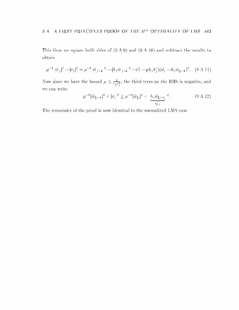
��A� A FIRST PRINCIPLES PROOF OF THE H� OPTIMALITY OF LMS ��
This time we square both sides of ���A��� and ���A� �� and subtract the results to
obtain
���j wjjj� � jvjj
� � ���j wjj��j� � jhj wjj��j
� � � � �hjh�j ��dj � hj �wjj���
�� ���A� �
Now since we have the bound � � �
hjh�j� the third term on the RHS is negative� and
we can write
���j wjj��j� � jvjj
� � ���j wjjj� � jhj wjj��� �z �
ep�j
j�� ���A� ��
The remainder of the proof is now identical to the normalized LMS case�

Chapter ��
Robustness of Least�Squares
Estimators
In the previous chapter we demonstrated that instantaneous�gradient�based adaptive
�lters� such as the LMS and normalized LMS algorithms� minimize the maximum
energy gain from the disturbances to the �prediction and �ltered� estimation errors�
A natural question to ask is how do other adaptive algorithms compare to these �H��
�optimal solutions Needless to say� in theH� approach to robust adaptive �ltering�
given any algorithm� this comparison is achieved by computing the corresponding
maximum energy gain �or H� norm� from the disturbances to the estimation errors�
In this chapter we shall study the robustness of the other important class of
adaptive �lters� namely� least�squares�based methods� such as the RLS algorithm�
from the above point of view� We shall essentially obtain upper and lower bounds for
theH� norm of the RLS algorithm �in fact� more generally� of the Kalman �lter� with
respect to prediction and �ltered errors� The main conclusion is that� unlike LMS
and normalized LMS which do not allow for any ampli�cation of the disturbances�
the RLS algorithm does allow for such ampli�cation� This fact can be especially
pronounced in the prediction error case� Moreover� it is shown that the H� norm for
RLS is data�dependent� whereas for LMS and normalized LMS it was not so� �The
H� norm was simply unity�� The signi�cance of the results will also discussed�
�

����� INTRODUCTION ��
���� Introduction
In the spirit of recent work in robust control there has been growing interest in deter�
ministic worst�case identi�cation� In such problems one is confronted with the task
of designing identi�cation algorithms that have robust performance in the presence
of unknown but bounded noise� Likewise it is required to analyze the worst�case be�
haviour of various identi�cation algorithms with respect to such disturbances� For an
introduction to recent approaches in H� and l� identi�cation the reader is referred
to �AHN��� WL��� DTT��� AK��� Mil��� PM��� and the references therein�
In the previous chapter we showed that the LMS �normalized LMS� adaptive
algorithm is H��optimal in the sense that it minimizes the worst�case energy gain
from the disturbances to the prediction ��ltered� errors� This result con�rmed the
robustness of LMS �normalized LMS� with respect to model uncertainties and gave
it a rigorous basis which was lacking� The celebrated recursive�least�squares �RLS�
algorithm �Hay���� is an also widely used adaptive algorithm that enjoys certain
well known optimality properties under suitable stochastic assumptions about the
exogenous noise� In Chapter � we also compared the robustness of the RLS algorithm
to LMS� and constructed a disturbance sequence of small energy for which RLS yielded
a prediction error of large energy�
In the present chapter we shall obtain upper and lower bounds on the H� norm
of the RLS algorithm� These bounds are of interest for several reasons� First they
demonstrate that unlike the LMS algorithm whose H� norm is unity �independent
of the input�output data�� the H� norm of the RLS algorithm depends on the input�
output data� and therefore it may be more robust or less robust with respect to
di�erent data sets� Moreover� the exact calculation of the H� norm for RLS requires
the calculation of the induced two�norm of a linear time�varying operator� which can
be quite cumbersome� and� in addition� needs all the input�output data� which may
not be available in real�time scenarios� The H� bounds we obtain only require simple
a priori knowledge of the data� and may therefore be used as a simple check to verify
whether RLS has the desired robustness with respect to a given application�
A brief outline of the chapter is as follows� In Sec� ���� we give general upper

�� CHAPTER ��� ROBUSTNESS OF LEAST�SQUARES ESTIMATORS
and lower bounds for the H� norm of the Kalman �lter� with respect to prediction
and �ltered errors� The proofs of the upper bounds are given in Sec� ���� and are
based on certain minimization properties of least�squares estimators� The proofs of
the lower bounds are given in ��� and are essentially based on computing the energy
gains for suitably chosen disturbances� Sec� ���� specializes the general results of Sec�
���� to the adaptive �ltering problem� discusses its various implications and provides
a simple example to illustrate the results� The chapter concludes with Sec� �����
���� A General H� Bound
In this section we shall derive general upper and lower bounds for the H� norm of the
Kalman �lter with respect to prediction and �ltered errors� These results will then
be specialized to the adaptive �ltering problem to obtain corresponding H� norm
bounds for the RLS algorithm�
To this end� consider� once more� the standard state�space model��� xi�� � Fixi �Giui� x�
yi � Hixi � vi� i � ���������
where Fi � Cn�n� Gi � Cn�m and Hi � Cp�n are known matrices� x�� fuig� and fvigare unknown quantities and yi is the measured output� Moreover� vi can be regarded
as measurement noise and ui as process noise or driving disturbance�
Recall from Chapter � that the Kalman �lter for computing the predicted esti�
mates of the states� denoted by �xi� �i�e�� �xi is the least�squares estimate of xi� given
fyj� j � ig� is given by
�xi�� � Fi�xi �Kp�i�yi �Hi�xi�� ��������
where
Kp�i � FiPiH�i R
��e�i and Re�i � Ri �HiPiH
�i ��������
and where Pi satis�es the Riccati recursion�
Pi�� � FiPiF�i �GiQiG
�i �Kp�iRe�iK
�p�i� P� � ��� ������ �
�Note here that fQi� Rig and �� are given positive de�nite weighting matrices��
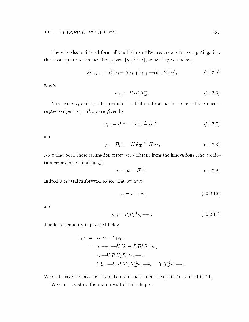
����� A GENERAL H� BOUND ��
There is also a �ltered form of the Kalman �lter recursions for computing� �xiji�
the least�squares estimate of xi� given fyj� j � ig� which is given below�
�xi��ji�� � Fi�xiji �Kf�i���yi�� �Hi��Fi�xiji�� ��������
where
Kf�i � PiH�i R
��e�i � ��������
Now using �xi and �xiji the predicted and �ltered estimation errors of the uncor�
rupted output� si � Hixi� are given by
ep�i � Hixi �Hi�xi�� Hi�xi� ��������
and
ef�i � Hixi �Hi�xiji�� Hi�xiji� ��������
Note that both these estimation errors are di�erent from the innovations �the predic�
tion errors for estimating yi��
ei � yi �Hi�xi� ��������
Indeed it is straightforward to see that we have
ep�i � ei � vi� ���������
and
ef�i � RiR��e�i ei � vi� ���������
The latter equality is justi�ed below�
ef�i � Hixi �Hi�xiji
� yi � vi �Hi��xi � PiH�i R
��e�i ei�
� ei �HiPiH�i R
��e�i ei � vi
� �Re�i �HiPiH�i �R
��e�i ei � vi � RiR
��e�i ei � vi�
We shall have the occasion to make use of both identities ��������� and ����������
We can now state the main result of this chapter�
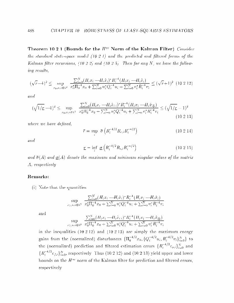
�� CHAPTER ��� ROBUSTNESS OF LEAST�SQUARES ESTIMATORS
Theorem ������ �Bounds for the H� Norm of the Kalman Filter� Consider
the standard state�space model �������� and the predicted and ltered forms of the
Kalman lter recursions �������� and ��������� Then for any N we have the follow�
ing results
�p�r���� � sup
x��u�v�h�
PNi���Hixi �Hi�xi��R��
i �Hixi �Hi�xi�
x������ x� �
PNi�� u
�iQ
��i ui �
PNi�� v
�iR
��i vi
� �p�r���� ���������
and
�q��r � ��� � sup
x��u�v�h�
PNi���Hixi �Hi�xiji��R��
i �Hixi �Hi�xiji�x���
��� x� �
PNi�� u
�iQ
��i ui �
PNi�� v
�iR
��i vi
� �q��r � ���
���������
where we have dened
�r � supi
���R����i Re�iR
����i
�������� �
and
r � infi
��R����i Re�iR
����i
����������
and ���A� and ��A� denote the maximum and minimum singular values of the matrix
A respectively�
Remarks�
�i� Note that the quantities
supx��u�v�h�
PNi���Hixi �Hi�xi��R��
i �Hixi �Hi�xi�
x������ x� �
PNi�� u
�iQ
��i ui �
PNi�� v
�iR
��i vi
and
supx��u�v�h�
PNi���Hixi �Hi�xiji��R��
i �Hixi �Hi�xiji�x���
��� x� �
PNi�� u
�iQ
��i ui �
PNi�� v
�iR
��i vi
in the inequalities ��������� and ��������� are simply the maximum energy
gains from the �normalized� disturbances f������ x�� fQ����
i ui� R����i vigNi��g to
the �normalized� prediction and �ltered estimation errors fR����i ep�igNi�� and
fR����i ef�igNi��� respectively� Thus ��������� and ��������� yield upper and lower
bounds on the H� norm of the Kalman �lter for prediction and �ltered errors�
respectively�

����� A GENERAL H� BOUND ��
�ii� Note� moreover� that the upper and lower bounds on the H� norms� as given
by Theorem ������ are relatively tight �especially for large values of �r and ��r��
Indeed the upper and lower bounds di�er only by two� since�
�p�r � ��� �
p�r � �� � � and �
q��r � �� � �
q��r � �� � ��
�iii� Note that Theorem ������ bounds the H� norm of the Kalman �lter by quan�
tities related to the maximum and minimum singular values of the normalized
innovations variance� R����i Re�iR
����i � Intuitively� ��������� suggests that the
larger Re�i is� the larger �r is� and hence the less robust the Kalman �lter is with
respect to prediction errors� On the other hand� ��������� suggests that the
smaller Re�i is� the larger ��r is� and hence the less robust the Kalman �lter is
with respect to �ltered errors�
In particular� note that
R����i Re�iR
����i � Ip �R
����i HiPiH
�i R
����i � Ip� ���������
so that
�r � � � ��r� ���������
But using ��������� this means that
supx��u�v�h�
PNi���Hixi �Hi�xiji��R��
i �Hixi �Hi�xiji�x���
��� x� �
PNi�� u
�iQ
��i ui �
PNi�� v
�iR
��i vi
� � ���������
which is a very explicit� and quite surprising� bound� Thus the Kalman �lter
guarantees that the energy gain from the disturbances to the �ltered errors
never exceeds four�
�iv� The bounds of Theorem ������ are true for any value of N � and� in fact� they
are also true when the upper limits of the sums in ��������� and ��������� are
in�nite� In other words� it is true that�
�p�r � ��� � sup
x��u�v�h�
P�i���Hixi �Hi�xi�
�R��i �Hixi �Hi�xi�
x������ x� �
P�i�� u
�iQ
��i ui �
P�i�� v
�iR
��i vi
� �p�r � ���
���������

�� CHAPTER ��� ROBUSTNESS OF LEAST�SQUARES ESTIMATORS
and
�q��r���� � sup
x��u�v�h�
P�i���Hixi �Hi�xiji��R
��i �Hixi �Hi�xiji�
x������ x� �
P�i�� u
�iQ
��i ui �
P�i�� v
�iR
��i vi
� �q��r����
���������
where� as before
�r � supi
���R����i Re�iR
����i
�and r � inf
i��R����i Re�iR
����i
��
In particular� in the time�invariant �doubly� in�nite�horizon case we have
�p�r� ��� � sup
x��u�v�h�
P�i����Hixi �Hi�xi��R���Hixi �Hi�xi�
x������ x� �
P�i��� u�iQ
��i ui �
P�i��� v�iR
��i vi
� �p�r����
���������
and
�q��r � ��� � sup
x��u�v�h�
P�i����Hxi �H�xiji��R���Hxi �H�xiji�P�
i��� u�iQ��ui �P�
i��� v�iR��vi� �
q��r � ���
���������
where now
�r � ���R����ReR
����� and r � ��R����ReR
����� � ���������
and Re � R �HPH�� with P the unique positive semide�nite and stabilizing
solution of the DARE
P � FPF ��GQG� � FPH��R �HPH����HPF ��
We will now proceed with the proof of Theorem �������
���� Proof of the Upper Bounds
To prove the upper bounds of Theorem ������ we need the following three facts�
Lemma ����� �Minimization of a Quadratic Form� We have
minx��fui�vig
x������ x� �
NXi��
u�iQ��i ui �
NXi��
v�iR��i vi �
NXi��
e�iR��e�i ei� ��������
where the minimization is taken subject to the state�space constraints �������� and
where ei � yi �Hi�xi is the innovations�

����� PROOF OF THE UPPER BOUNDS ��
Proof� The lemma is simply a special case of Theorem ���� �
Lemma ����� �Simple Inequality� For any vectors a b and any matrix M � �
we have
�a� b��M�a� b� � �� � �
��a�Ma� �� � ��b�Mb� �� � �� ��������
Proof� Follows from
�a� b��M�a� b�� ��� �
��a�Ma� ��� ��b�Mb �
�
�a�Ma� a�Mb� b�Ma� �b�Mb
� ��p�a�
p�b��M�
�p�a�
p�b�
� ��
Lemma ���� �A Simple Minimization� For all � � we have
min���
�� � � � ���
�� �� �� �
q��� ��������
and
argmin���
�� � � � ���
�� �� � �
q� ������ �
Proof� Readily veri�ed via di�erentiation�
We shall �rst prove the upper bound in ��������� for the prediction error case� To
this end� de�ne
J � x������ x� �
NXi��
u�iQ��i ui �
NXi��
v�iR��i vi� ��������
Now using Lemma ������ it is obvious that
J � minx� �fui�vig
J �NXi��
e�iR��e�i ei� ��������

�� CHAPTER ��� ROBUSTNESS OF LEAST�SQUARES ESTIMATORS
Thus we may write�
J �NXi��
e�iR��e�i ei
�NXi��
e�iR����i R
���i R��
e�iR���i R
����i ei
�NXi��
��R���i R��
e�iR���i
�e�iR
��i ei
��infi
���R���i R��
e�iR���i
�� NXi��
e�iR��i ei
�
�sup
i
�
����R����i Re�iR
����i
�� NXi��
e�iR��i ei
��
�r
NXi��
e�iR��i ei
��
�r
NXi��
�ep�i � vi��R��
i �ep�i � vi� using ���������
Now using Lemma �������� with a � ep�i� b � vi and M � R��i � we have
x������ x� �
NXi��
u�iQ��i ui �
NXi��
v�iR��i vi � �
�r
NXi��
���� ��v�iR
��i vi � ��� �
��e�p�iR
��i ep�i
��
��������
for any � � �� Now rearranging terms� we can write
��� �
��
NXi��
e�p�iR��i ep�i � �rx���
��� x���r
NXi��
u�iQ��i ui��r��� � � �
�r�
NXi��
v�iR��i vi� ��������
so that� assuming � � �� we have
NXi��
e�p�iR��i ep�i � �r
� � �
�
�x���
��� x� �
NXi��
u�iQ��i ui
�
�r
� � �
�
��� � � �
�r�
NXi��
v�iR��i vi
��r
� � �
�
�x���
��� x� �
NXi��
u�iQ��i ui
��� � ���r � ��
� � �
NXi��
v�iR��i vi�
To obtain the �tightest possible bound onPN
i�� e�p�iR
��i ep�i� let us minimize� over
� � �� the coe�cient ofPN
i�� v�iR
��i vi on the RHS of the above inequality� But from
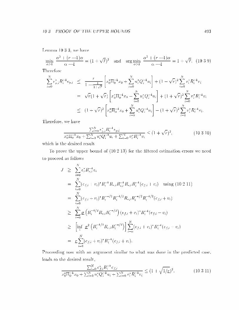
����� PROOF OF THE UPPER BOUNDS ��
Lemma ������� we have
min���
�� � ��r � ���
� � �� �� �
p�r�� and argmin
���
�� � ��r � ���
�� �� � �
p�r� ��������
ThereforeNXi��
e�p�iR��i ep�i � �r
�� �
��p�r
�x���
��� x� �
NXi��
u�iQ��i ui
� �� �
p�r��
NXi��
v�iR��i vi
�p�r�� �
p�r�
�x���
��� x� �
NXi��
u�iQ��i ui
� �� �
p�r��
NXi��
v�iR��i vi
� �� �p�r��
�x���
��� x� �
NXi��
u�iQ��i ui
� �� �
p�r��
NXi��
v�iR��i vi�
Therefore� we have PNi�� e
�p�iR
��i ep�i
x������ x� �
PNi�� u
�iQ
��i ui �
PNi�� v
�iR
��i vi
� �� �p�r��� ���������
which is the desired result�
To prove the upper bound of ��������� for the �ltered estimation errors we need
to proceed as follows�
J �NXi��
e�iR��e�i ei
�NXi��
�ef�i � vi��R��
i Re�iR��e�iRe�iR
��i �ef�i � vi� using ���������
�NXi��
�ef�i � vi��R����
i R����i Re�iR
����i R
����i �ef�i � vi�
�NXi��
��R����i Re�iR
����i
��ef�i � vi�
�R��i �ef�i � vi�
��infi
���R����i Re�iR
����i
�� NXi��
�ef�i � vi��R��
i �ef�i � vi�
� rNXi��
�ef�i � vi��R��
i �ef�i � vi��
Proceeding now with an argument similar to what was done in the predicted case�
leads ro the desired result�PNi�� e
�f�iR
��i ef�i
x������ x� �
PNi�� u
�iQ
��i ui �
PNi�� v
�iR
��i vi
� �� �q��r��� ���������

� CHAPTER ��� ROBUSTNESS OF LEAST�SQUARES ESTIMATORS
���� Proof of the Lower Bounds
Perhaps the most general way of computing the a lower bound for the H� norm of
RLS� or any other algorithm for that matter� is to compute the energy gain for some
particular choice of disturbance signal� fx�� fui� vigNi��g�� We shall presently see that
the special choice of disturbance signal that yields the lower bound of Theorem ������
is that disturbance signal that minimizes the quadratic form
J � x������ x� �
NXi��
u�iQ��i ui �
NXi��
v�iR��i vi� ���� ���
subject to the state�space constraints ��������� To facilitate the presentation of the
proof it will be convenient to make the following de�nitions�
y��
��������
y�
y����
yN
��������
� u��
��������
u�
u����
uN
��������
� v��
��������
v�
v����
vN
��������
���� ���
and
e��
��������
y� �H��x�
y� �H��x����
yN �HN �xN
��������
� ep��
��������
H�x� �H��x�
H�x� �H��x����
HNxN �HN �xN
��������
� ef��
��������
H�x� �H��x�j�H�x� �H��x�j�
���
HNxN �HN �xN jN
���������
���� ���
Moreover� from Chapter � we know that the innovations� e� can be found via
e � L��y� ���� � �
where L is a lower triangular matrix with unit diagonal that is given from the unique
�block� LDU decomposition�
Ry � LReL�� ���� ���
�The resulting energy gain will be less than or equal to the maximum energy gain and hence alower bound to the �squared� H� norm�

����� PROOF OF THE LOWER BOUNDS ��
where
Re � diag�Re��� Re��� � � � � Re�N �� ���� ���
and Ry� the output Gramian� is given by
Ry � O��O� � �Q�� �R� ���� ���
where
O �
��������
H�
H�F����
HNFN�� � � F�
��������� ���� ���
is the observability map� and
� �
����������
�
H�G� �
H�F�G� H�G� �
H�F�F�G� H�F�G� H�G� �
� � � � �
����������� ���� ���
is the impulse response matrix� and
Q�� diag�Q�� Q�� � � � � QN � and R
�� diag�R�� R�� � � � � RN �� ���� ����
Finally� we need to note the global relation�
y � Ox� � �u � v� ���� ����
and� using ��������� and ���������� the relations
ep � e� v � L��y � v� ���� ����
and
ef � RR��e e� v � RR��
e L��y � v� ���� ����
Now note that� using a completion of squares argument� we can write
J � x������ x� � u�Q��u� �y �Ox� � �u��R���y �Ox� � �u�
�hx�� � �x��jN u� � �u�jN
i � ����
Q��
�� x� � �x�jN
u� �ujN
�� y�R��
y y�
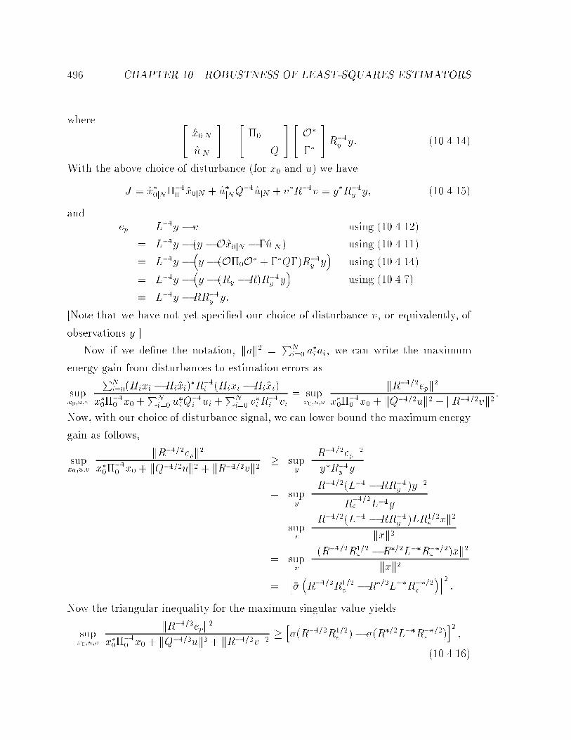
�� CHAPTER ��� ROBUSTNESS OF LEAST�SQUARES ESTIMATORS
where � �x�jN
�ujN
� �
� ��
Q
�� O�
��
�R��
y y� ���� �� �
With the above choice of disturbance �for x� and u� we have
J � �x��jN���� �x�jN � �u�jNQ
���ujN � v�R��v � y�R��y y� ���� ����
andep � L��y � v using ���� ����
� L��y � �y �O�x�jN � ��ujN � using ���� ����
� L��y ��y � �O��O� � ��Q��R��
y y�
using ���� �� �
� L��y ��y � �Ry �R�R��
y y�
using ���� ���
� L��y �RR��y y�
�Note that we have not yet speci�ed our choice of disturbance v� or equivalently� of
observations y��
Now if we de�ne the notation� kak� �PN
i�� a�iai� we can write the maximum
energy gain from disturbances to estimation errors as
supx��u�v
PNi���Hixi �Hi�xi�
�R��i �Hixi �Hi�xi�
x������ x� �
PNi�� u
�iQ
��i ui �
PNi�� v
�iR
��i vi
� supx��u�v
kR����epk�x���
��� x� � kQ����uk� � kR����vk� �
Now� with our choice of disturbance signal� we can lower bound the maximum energy
gain as follows�
supx��u�v
kR����epk�x���
��� x� � kQ����uk� � kR����vk� � sup
y
kR����epk�y�R��
y y
� supy
kR�����L�� �RR��y �yk�
R����e L��y
� supx
kR�����L�� �RR��y �LR���
e xk�kxk�
� supx
k�R����R���e �R���L��R����
e �xk�kxk�
�h���R����R���
e �R���L��R����e
�i��
Now the triangular inequality for the maximum singular value yields
supx��u�v
kR����epk�x���
��� x� � kQ����uk� � kR����vk� �
h���R����R���
e �� ���R���L��R����e �
i��
���� ����

����� PROOF OF THE LOWER BOUNDS ��
Moreover� note that we have
���R����R���e � �
q���R����ReR�����
�
r���diag�R
����� Re��R
����� � � � � R
����N Re�NR
����N �
�
�
ssupi
���R����i Re�iR
����i �
�pr� ���� ����
and
�R���L��R����e ��R����
e L��R���� � R���R��y R���
� �I �R����O��O�R���� �R�����Q��R�������
� I�
so that
���R���L��R����e � � �� ���� ����
Combining Eqs� ���� ����� ���� ���� and ���� ���� yields the desired result�
supx��u�v
PNi���Hixi �Hi�xi��R��
i �Hixi �Hi�xi�
x������ x� �
PNi�� u
�iQ
��i ui �
PNi�� v
�iR
��i vi
� �pr � ���� ���� ����
The proof of the lower bound for �ltered errors is very similar� The only di�erence
is that here we need to compute ef in terms of y �for our choice of disturbances as
given by ���� �� ��� In this case
ef � RR��e e� v � RR��
e L��y �RR��y y� ���� ����
Thus we now have
supx��u�v
kR����efk�x���
��� x� � kQ����uk� � kR����vk� � sup
y
kR����efk�y�R��
y y
� supy
kR�����RR��e L�� �RR��
y �yk�R����e L��y
� supx
kR�����RR��e L�� �RR��
y �LR���e xk�
kxk�

�� CHAPTER ��� ROBUSTNESS OF LEAST�SQUARES ESTIMATORS
� supx
k�R���R����e �R���L��R����
e �xk�kxk�
�h���R���R����
e �R���L��R����e
�i��
h���R���R����
e �� ���R���L��R����e �
i��
�q��r � �
���
where in the last step we used the �readily veri�able� fact that
���R���R����e � �
q��r� ���� ����
But this is our desired result�
���� RLS Adaptive Filtering
We are now in a position to specialize the result of Theorem ������ to the case of
adaptive �ltering� Recall that in adaptive �ltering the model is given by
di � hTi w � vi� ��������
where di is the observation� hTi �hhi� hi� � � � hin
iis a known ��n input vector�
w is the unknown weight vector that we intend to estimate� and vi is an unknown
disturbance signal�
As mentioned earlier in Secs� ����� and Sec� ���� the adaptive �ltering problem is
a special case of a state�space estimation problem �see the state�space model ���������
resulting from the parameters�
Fi � In � Gi � � � Hi � hTi � Ri � Ip� ��������
The RLS �recursive�least�squares� algorithm is essentially the Kalman �lter corre�
sponding to a state�space model with the above system matrices� Thus the least�
squares estimates �wji �of the weight vector w� using the observations� fdj � j � ig�obey the following recursions�
�wji � �wji�� � kp�i�di � hTi �wji���� �w � ��������

����� RLS ADAPTIVE FILTERING ��
where
kp�i �Pihi
� � hTi Pihi� ������ �
and Pi satis�es the Riccati recursion�
Pi�� � Pi � PihihTi Pi
� � hTi Pihi� P� � I� ��������
It is also useful to remark that at each time instant� i� the above RLS algorithm
solves the following least�squares problem�
minw
���jw � �wj��j� �
iXj��
jdj � hTj wj�� � ��������
where ��jw�w��j� is a possible regularization term that re ects a priori knowledge
as to how close w is to the initial estimate w��� The special case where mu ��� so
that the �rst term in the cost function of �������� disappears� is referred to as a pure
least�squares problem� We will shortly have more to say about such problems�
As before let us de�ne the following prediction and �ltered estimation errors�
ep�i � hTi w � hTi �wji��� ��������
and
ef�i � hTi w � hTi �wji��� ��������
It will also be useful to de�ne the following smoothed estimation error �since we know
from Sec� �� that least�squares smoothers are H� optimal��
es�i � hTi w � hTi �wjN � i � �� � � � � N� ��������
The following result is now immediate�
Theorem ����� �Bounds for the H� Norm of the RLS Algorithm� Consider
the adaptive ltering model �������� and the least�squares estimates �wji given by the
RLS algorithm ��������� Then for any N we have the following results
�p�r � ��� � sup
w�v�h�
PNi���h
Ti w � hTi �wji���
��hTi w � hTi �wji�����jw � �wj��j� �PN
i�� v�iR
��i vi
� �p�r � ��� ���������

��� CHAPTER ��� ROBUSTNESS OF LEAST�SQUARES ESTIMATORS
�q��r � ��� � sup
w�v�h�
PNi���h
Ti w � hTi �wji�
��hTi w � hTi �wji���jw � �wj��j� �PN
i�� v�iR
��i vi
� �q��r � ��� ���������
and
supw�v�h�
PNi���h
Ti w � hTi �wjN�
��hTi w � hTi �wjN ���jw � �wj��j� �PN
i�� v�iR
��i vi
� � ���������
where we have dened
�r � supi
h� � hiPih
Ti
i� ���������
and
r � infi
h� � hiPih
Ti
i� ������� �
Proof� The proof of the bounds ��������� and ��������� follow immediately from
Theorem ������ when the systemmatrices are appropriately specialized� Eq� ���������
follows from the H� optimality of least�squares smoothers� as given by Sec� �� � and
by the results of Chapter � on H��optimal adaptive �lters�
In the RLS algorithm the it is easy to solve �������� to obtain Pi � ���I �Pi��j�� hjh
Tj ���� which implies that the Pi are a monotonically decreasing sequence of
matrices� If we assume that the input vectors hi have equal magnitude �i�e� hTi hi �
const�� then we have the following result�
Corollary ����� �Constant Magnitude Inputs� If the input vectors have con�
stant magnitude hTi hi � �h� then
�q� � �h�� ��� � sup
w�v�h�
PNi���h
Ti w � hTi �wji���
��hTi w � hTi �wji�����jw � �wj��j� �PN
i�� v�iR
��i vi
� �q� � �h������
���������
The following is also straightforward�
Corollary ����� If �h��� supi h
Ti hi and h�
�� infi hTi hi then
�q� � h�� ��� � sup
w�v�h�
PNi���h
Ti w � hTi �wji���
��hTi w � hTi �wji�����jw � �wj��j� �PN
i�� v�iR
��i vi
� �q� � �h������
���������

����� RLS ADAPTIVE FILTERING ���
Finally� the following result for �ltered errors is also immediate and follows readily
from the expression Pi � ���I �Pi��
j�� hjhTj ����
Corollary ���� We have
limi��
r � �� ���������
so that
supw�v�h�
PNi���h
Ti w � hTi �wji�
��hTi w � hTi �wji���jw � �wj��j� �PN
i�� v�iR
��i vi
� � ���������
Remarks�
�i� Corollary ������ has an interesting interpretation! for large values of � the RLS
algorithm is less robust with respect to prediction errors� In fact� we see that
the �upper and lower bounds of the�H� norm grows asp� This is reminiscent
of the robustness properties of LMS� where� as shown in Chapter �� the learning
rate had to be small enough to guarantee H� optimality�
More importantly� Corollary ������ shows that the pure least�squares problem
�corresponding to � �� can be highly nonrobust with respect to prediction
errors�
�ii� From Corollary ������� for �ltered errors� the RLS algorithm yields�
supw�v�h�
kefk����jw � �wj��j� � kvk�
�
� �
Note that� as with the normalized LMS algorithm� the H� norm does not
depend on �
The above result shows that� for �ltered errors� least�squares algorithms are
at most four times worse than H��optimal algorithms �where �opt � ��� This
demonstrates an intermediate stage between the smoothed error case �which
has access to all the observations� and where the H� and H� optimal �lters
coincide� and the prediction error case �which does not have access to current
observations� and where the performance of LMS and RLS can be drastically
di�erent��
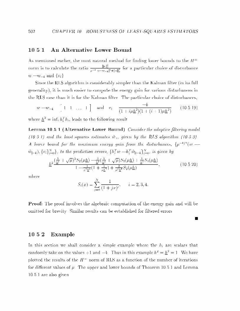
��� CHAPTER ��� ROBUSTNESS OF LEAST�SQUARES ESTIMATORS
������ An Alternative Lower Bound
As mentioned earlier� the most natural method for �nding lower bounds to the H�
norm is to calculate the ratio kek��
���jw�w��j��kvk��
for a particular choice of disturbance
w � w�� and fvig�Since the RLS algorithm is considerably simpler than the Kalman �lter �in its full
generality�� it is much easier to compute the energy gain for various disturbances in
the RLS case than it is for the Kalman �lter� The particular choice of disturbances�
w � w�� �h� � � � � �
iand vi �
���� � ih���� � �i� ��h��
���������
where h� � infi hTi hi� leads to the following result�
Lemma ����� �Alternative Lower Bound� Consider the adaptive ltering model
�������� and the least�squares estimates �wji given by the RLS algorithm ���������
A lower bound for the maximum energy gain from the disturbances f�����w ��wj���� fvigNi��g to the prediction errors fhTi w � hTi �wji��gNi�� is given by
h�� �
h��p��S��h�� �
h�� �
h��p�S��h� �
�
h�S�h�
�� �
��h��� � �
�h�� � �
��h�S��h�
� ���������
where
Si�x� �NXj��
�
�� � jx�i� i � �� �� �
Proof� The proof involves the algebraic computation of the energy gain and will be
omitted for brevity� Similar results can be established for �ltered errors�
������ Example
In this section we shall consider a simple example where the hi are scalars that
randomly take on the values �� and ��� Thus in this example �h� � h� � �� We have
plotted the results of the H� norm of RLS as a function of the number of iterations
for di�erent values of � The upper and lower bounds of Theorem ������ and Lemma
������ are also given�

���� CONCLUSION ���
0 2 4 6 81
1.5
2
2.5
log(N)
mu = .9
0 20 40 601
1.5
2
2.5
3
N
mu = 2
0 20 40 602
2.5
3
3.5
N
mu = 5
0 20 40 603
3.5
4
4.5
N
mu = 10
Figure ����! H� norm of RLS as a function of the number of data points and as afunction of � The upper and lower bounds of Theorem ������ and Lemma ������ aregiven by the horizontal lines� As can be seen from the �gures� in this example� thelower bounds of Lemma ������ seem quite accurate for large �
���� Conclusion
In this chapter we obtained upper and lower bounds for the H� norm of the RLS
algorithm� These bounds may be used to study the robustness of RLS in di�erent
applications� Our results show that theH� norm of RLS depends on the input�output
data �viz� on the fhig�� as opposed to the LMS and normalized LMS algorithms
where the H� norm is independent of the data� The bounds further show that� for
prediction errors� the H� norm of RLS grows as the square�root of �where ��I is
the regularization term in least�squares problems that re ects a priori knowledge of
the weight vector�� whereas for �ltered errors� the H� norm of RLS �and the Kalman

�� CHAPTER ��� ROBUSTNESS OF LEAST�SQUARES ESTIMATORS
�lter� is bounded by two� Simulations show that the bounds are quite reasonable
compared to the true computed H� norms�

Chapter ��
H� Adaptive Filtering
The previous two chapters were more or less concerned with the study of adaptive
�lters from an H� point of view� Chapter � studied the problems of output predic�
tion and output �ltered estimation in adaptive �ltering� using an H� approach� and
demonstrated the H� optimality of the LMS and normalized LMS algorithms with
respect to these two estimation criteria� Chapter �� studied the robustness of least�
squares�based adaptive �lters� such as the RLS algorithm� using the H� framework�
A reading of Chapters � and �� indicates that there may be great promise in the
interplay of adaptive �ltering and H� estimation theory�
To round up the story� in this chapter� we shall present a preliminary study of the
design of adaptive �lters using an H� criterion� The strength of H��optimal adaptive
�lters lies in the fact that they guarantee the smallest possible estimation error energy
over all possible disturbances of �xed energy� and are therefore robust with respect
to model uncertainties and lack of statistical information on the exogenous signals�
Speci�cally� in this chapter we study the problem of prediction of the weight vector
itself� and for the purpose of coping with time�variations� exponentially weighted�
�nite�memory and time�varying adaptive �ltering� This results in some new adaptive
�ltering algorithms that may be useful in uncertain and non�stationary environments�
We should mention that the presentation of this chapter is deliberately brief� The
main reasons are that the results given here are preliminary� and that we believe the
area is worthy of much more scrutiny and study� Indeed� we have just scratched the
�
� CHAPTER ��� H� ADAPTIVE FILTERING
surface� The main goal� therefore� has been to hint at the possibilities�
���� Introduction
Since its inception in the early ����s �WH�� GWW� adaptive �ltering has been
widely used to cope with time�variations of system parameters and lack of a priori
knowledge of the statistical properties of the input data� This is in contrast to Wiener
and Kalman �lter theory which require a priori statistical information� Early suc�
cesses of adaptive �ltering were in channel equalization for digital communications
�Luc and in adaptive antennas �How� App� Wid� � Currently� recent advances
in ASIC�s �application�speci�c processors� and sensor technology have spurred an in�
creasing range of applications from biomedical engineering to wireless communica�
tions� so that there is still great interest in the �eld�
Although there have been several successful applications of adaptive �ltering� it is
fair to say that most of the results are empirical and that there still is not an adequate
theoretical basis for the analysis of the performance of these algorithms � limits of
performance� sensitivity� optimality� etc� �The basic reason is that adaptive systems
are inherently time�variant and nonlinear�� Much work has been done in this area in
control theory� especially in adaptive control� though many questions still remain�
Due to the similarity between the objectives of adaptive �ltering �coping with
time�variations� insensitivity to lack of statistical knowledge� etc�� and H� estimation
�robustness with respect to uncertainties in the underlying model and�or statistics��
it is expected that there should be some connection between the two� Indeed� we have
seen in Chapter that the celebrated LMS algorithm �WH� � which is widely used in
adaptive �ltering� is H� optimal� This result gives more insight into the inherent
robustness of the LMS algorithm and why it has found such wide applicability in such
a diverse range of problems� As a matter of fact� we believe that the H� approach
yields a new way of looking at adaptive systems� and has several rami�cations� as
well as suggesting directions for further research�
In this chapter we further pursue the connections between adaptive �ltering and
H� estimation� In particular� we consider predicting the complete �lter weight vector

����� INTRODUCTION ��
which leads to a new adaptive algorithm� We also develop a host of H� algorithms
to deal with time�variations and non�stationary signals� Two of these algorithms
are based on exponentially weighted and �nite memory windows� respectively� and
a third algorithm allows for general time variations in the underlying �lter weight
vector� The goal of this chapter is to outline the use of the H� criterion in the design
adaptive �lter algorithms� There are� no doubt� a wide variety of other H� adaptive
algorithms �not considered here� that could be worthy of further scrutiny�
Important Remark
At this point we should make an important remark on the contribution of this chapter�
As is wellknown� once an upper bound on the value of � that ensures the existence
of an H� �lter is given� the structure of the adaptive �lters readily follow from the
standard solution to the H� estimation problem �see e�g�� Chapter ��� Therefore�
since adaptive �ltering is just a special case of state�space estimation� that has been
solved �in its full generality� in the H� framework� it appears that there is not much
more to be done or said�
However� we should note that �nding the optimum value of � essentially amounts
to �nding the maximum singular value of a linear time�varying operator� Bounds on
� can be found by checking for the positivity of the solution of a certain time�varying
discrete�time Riccati recursion� Although both approaches can be used in principle�
they require knowledge of all the input data vectors fhig�
Since in adaptive �ltering problems we are given� and are forced to process� the
data in real time� we do not have the luxury of storing all the data and computing
explicit bounds for � using the aforementioned methods� Therefore the main e�ort in
H� adaptive �ltering is to obtain bounds on � that use simple a priori knowledge of
the fhig and not their explicit values� This is what is done in the results given below�
�� CHAPTER ��� H� ADAPTIVE FILTERING
���� Full Weight Vector Estimation
As mentioned in earlier chapters� in adaptive �ltering we assume that we observe an
output sequence fdig that obeys the following linear �lter model
di � hTi w � vi� ��������
where hTi �hhi� hi� � � � hin
iis a known input vector� w is the unknown �l�
ter weight vector that we intend to estimate� and fvig is an unknown disturbance
sequence that may include modeling errors� Let �wji � Fi�d�� d�� � � � � di� denote the
estimate of the weight vector given the inputs fhjg and the outputs fdjg from time
� up to and including time i�
InH� estimation the structure of the estimator depends on the linear combination
of the state �in our case the linear combination of the weight vector� that we intend
to estimate� This is as opposed to H� estimation where the estimate of any linear
combination of the state is simply that linear combination of the state estimate�
In Chapters � and �� our concern was prediction of the �lter output� which cor�
responds to the linear combination hTi w� Although in many applications predicting
the output of the �lter su�ces� in some applications �especially those concerned with
identi�cation� we are interested in estimating the weight vector itself� In this case we
de�ne the weight vector estimation error as
�wji � w � �wji� ��������
and we are concerned with the transfer operator Ts�N � from the disturbances fw �
�wj��� fvigNi��g to the weight estimation errors f �wjig
Ni��� The H
� full weight vector
estimation problemmay now be formulated as follows� where we have de�ned k �w k���PNi�� �w
Tji �wji�
Problem ������ �Optimal Weight Estimation Problem� Find an H��optimal
estimation strategy �wji � Fi�d�� d�� � � � � di� that minimizes kTs�Nk�� and obtain the
resulting
��s � infF
kTsk�� � infF
supw�v�h�
k �wk�����jw � w��j� � kvk
��
��������

����� FULL WEIGHT VECTOR ESTIMATION ��
where jw�w��j� � �w�w���T �w�w���� and � is a positive constant that re�ects a
priori knowledge as to how close w is to the initial guess w���
Before stating the solution to the above problem we need to de�ne the sample
covariance matrix of the input vectors fhjgi��j�� as follows
Ri ��
i
i��Xj��
hjhTj � ��������
Theorem ������ �Full Weight Estimator� Consider the model �������� and sup�
pose we wish to minimize the H� norm of the transfer operator� Ts�N � from the un�
knowns w � w�� and fvigNi�� to the weight vector estimation errors �wji� Then
�s � supi
vuut ���i� ��Ri�
� �������
where ��Ri� denotes the minimum singular value of Ri� The central optimal H�
estimator is given by
�wji � �wji�� �Pihi
� � hTi Pihi�di � hTi �wji���� w�� �������
where Pi satises the recursion
P��i�� � P��
i � hihTi � ���s I� P��
� � �I� ��������
Proof� The proof is a direct application of Theorem ����� on a posteriori state�space
H� estimators for the special state�space model
Fi � I � Gi � � � Hi � hTi � Li � In ��������
which corresponds to the adaptive �ltering model ��������� Note that we have taken
Li � In since the desired combination of the weights is the identity matrix �i�e�� we
want to estimate w itself�� Now from Theorem ����� if an estimator of level �s exists�
then the solution is given by ������� and ��������� Therefore all that remains to be
shown is the condition for the existence of the �lter�

�� CHAPTER ��� H� ADAPTIVE FILTERING
But according to Theorem ����� this condition is
P��i�� � P��
i � hihTi � ���s I � �� i � �� �� � � � N� ��������
Now the above Riccati equation can be solved to yield�
P��i�� � ���I �
iXj��
hjhTj � �i� ���
��s I�
� ���I � �i� ��Ri�� � �i� �����s I�
so that the condition for P��i�� � � becomes
Ri�� � ���s I ��
��i� ��I�
or
��Ri��� � ���s ��
��i� ��� ���������
Rearranging the above inequality yields�
�s �
vuut ���i� ��Ri�
� i � �� �� � � � N ���������
from which we obtain the desired result ��������
Remarks�
�i� It is interesting to compare the algorithm of Theorem ������ with the RLS
algorithm of Chapter ��� The only di�erence is that the covariance update in
RLS can be written as P��i�� � P��
i � hihTi � Due to this covariance update� Pi
�and hence the gain vector� may approach zero for large i� However� in the
algorithm of Theorem ������ the covariance update is more conservative and Pi
does not tend to zero meaning that we always have a non�zero gain vector� This
is similar to some ad�hoc schemes that are employedwith RLS to guarantee that
the gain vector does not go to zero �see �Hay� ��
�ii� It is interesting to note that ��Ri�� the minimum singular value of Ri� appears
in the bound for �s� Indeed if ��Ri� � �� then �s grows unbounded as time

����� TIME�VARIATION ��
progresses to in�nity� This makes perfect sense� since ��Ri� � � means that
the sample covariance matrix Ri ��i
Pi��j�� hjh
Tj is singular� i�e�� that there are
certain directions which the input vectors fhig do not �persistently� excite� In
such a case it will not be possible to estimate w along those directions� and
hence �s will tend to in�nity�
�iii� If the components of the input vectors fhig are independent random variables
with variance ��� then provided �� � �� for large i the algorithm of Theorem
������ reduces to
�wji � �wji�� ��
�� ���
hi
� � �
����hTi hi
�di � hTi �wji���� �wj�� ���������
which is the so�called normalized LMS algorithm with parameter �
���� �
���� Time�Variation
The H� adaptive �lters developed in Chapter � and the previous section are robust
with respect to model uncertainties and lack of statistical information on the exoge�
nous signals� However� since we have assumed the underlying model to be stationary
�we have taken the unknown weight vector as time�invariant� these algorithms may
not have desirable tracking properties in the face of time variations�
In this section we shall incorporate provisions to cope for time variations in the
underlying model� The methods used are similar to those used in the usual H� setting�
and here we generalize them to the H� setting� Although this can be done for both
the output estimation case and the full weight vector case� for brevity we shall only
consider the former�
������ Exponentially�Windowed Adaptive Filtering
One method to account for time�variations is to introduce a forgetting factor � �
� �� and to exponentially weight the energies with this forgetting factor� In this
manner the more recent data will be given larger weights than the earlier ones� This

�� CHAPTER ��� H� ADAPTIVE FILTERING
will allow the algorithms to track the time�variations of the underlying models� In
particular� the prediction error and disturbance energies are computed as�
NXj��
�ijep�ij� and
NXj��
�ijvij�� ��������
The forgetting factor � � � � is chosen based upon a priori knowledge of how fast
the weight vector varies with time�
Now for any choice of estimator F � we shall denote by T��N�F� the transfer op�
erator from the disturbances f���
� �w � �wj���� f� i� vigNi��g to the prediction errors
f�i� ep�igii�M � The H
� output prediction problem with exponential weighting can
thus be formulated as follows�
Problem ������ �ExponentiallyWindowed Problem� Find an H��optimal es�
timation strategy wi � F�d�� d�� � � � � di� that minimizes kT��Nk�� and obtain the re�
sulting
��� � infF
kT��Nk�� � infF
supw�v�h�
PNi�� jep�ij
��i
���jw � w��j� �PN
i�� jvij��i
��������
where jw � w��j� � �w � w���T �w � �wj���� and � is a positive constant that re�ects
a priori knowledge as to how close w is to the initial guess �wj���
Before giving the solution to the above problem we need the following de�nitions
�h�� sup
i
hTi hi � h�� inf
ihTi hi ��������
and
R��i��ii��Xj��
�jhjhTj � ��������
Theorem ������ �ExponentiallyWindowed Algorithm� Consider the model ��������
and suppose we wish to minimize the H� norm of the transfer operator T��N of Prob�
lem ������� Then
��� � supi
�h� ��R��i��i
�� ��R��i�
i � �� �� � � � N �������

����� TIME�VARIATION ��
and the central H��optimal estimator is given by
�wji � �wji�� ��Pihi
� � hTi�Pihi
�di � hTi �wji���� �wj�� �������
where �Pi satises the recursion
�P��i�� � �P��
i � hihTi � ���� hi��h
Ti���
�P��� � ���I � ���� h�h
T� � ��������
Proof� The proof is a direct application of Theorem ����� on a priori H� estimation
as applied to a Krein space state�space model with
Fi � I � Hi �
�� hTi
hTi
�� � Gi � � � � � �I � Ri �
�� � �
� ����
��i ��������
and with x� � w� Therefore� using Theorem ������ assuming a solution exists� the
solution is given by
�xi�� � �xi � �Pihi�i � hTi
�Pihi����di � hTi �xi�� �x� � �wj�� ��������
or� since xi � w� for all i
�wji � �wji�� � �Pihi�i � hTi
�Pihi����di � hTi �wji���� �wj�� ���������
where
�P��i � P��
i � ���� �ihihTi � ���������
and where Pi satis�es the Riccati recursion
Pi�� � Pi�Pihhi hi
i����� � �
� ����
��i �
�� hTi
hTi
��Pi h hi hi
i��� �� hTi
hTi
��Pi� P� � �I�
���������
Therefore we have
P��i�� � P��
i � ��� ���� ��ihih
Ti � P��
� � ���I ���������
so that
�P��i�� � �P��
i � �ihihTi � ���� �i��hi��h
Ti���
�P��� � ���I � ���� h�h
T� � ���������
�� CHAPTER ��� H� ADAPTIVE FILTERING
Now if we de�ne
�Pi � �i �Pi� ��������
we see that the recursion for �wji becomes
�wji � �wji�� ��Pihi
� � hTi�Pihi
�di � hTi �wji���� �wj�� ��������
which is precisely �������� and� moreover� �Pi satis�es the recursion
�P��i�� � �P��
i � hihTi � ���� hi��h
Ti���
�P��� � ���I � ���� h�h
T� � ���������
which is precisely ���������
Therefore all that remains to be shown is the existence condition for the �lter�
But from Theorem ����� this existence condition is
�Pi � �� i � �� �� � � � N� ���������
Now the recursion ��������� can be solved for �Pi to yield
�P��i�� � ���I �
iXj��
�� � ���� ��jhjh
Tj � ���� �i��hi��h
Ti��
� ���I � �� � ���� ��i��R��i�� � ���� �i��hi��h
Ti���
Therefore the condition �Pi�� � � implies
���I � ��� ���� ��i��R��i�� � ���� �i��hi��h
Ti���
or� equivalently�
�� � ���� �R��i�� � ���� hi��hTi�� �
i��
�I� ���������
A su�cient condition for the above inequality is that
�� � ���� ���R��i��� � ���� ���hi��hTi����
i��
�
� �����h�
i��
��
Rearranging this last expressions leads to
��� ��h� ��R��i���
�i��
�� ��R��i���
���������

����� TIME�VARIATION �
which yields the desired result ��������
Remarks�
�i� It is interesting to note that ��R��i�� the minimumsingular value of R��i� appears
in the bound for ��� Moreover� it follows from ������� that if ��R��i� � �� then
�� grows unbounded as time progresses to in�nity�
�ii� For large i the bound in ������� becomes
��� � � ��h
��R��i�� ���������
Note that for � �� we have ��R��i��� so that we are reduced to the bound
� � � of H� output prediction adaptive �ltering �that was solved by LMS��
Therefore the extra term�h
��R��irepresents the increase in the H� norm we
must incur due to the time�varying nature of the problem�
�iii� There is a similar exponentially�windowed a posteriori solution that can be
constructed for �ltered errors� However� for brevity we shall not do so here�
������ Finite�Memory Adaptive Filtering
Another approach for dealing with time�variations is the so�called sliding or �nite�
memory window� In this case one only considers data over a �nite window of length
L� Therefore as each new data is observed� the least recent data point is discarded so
that we have a memory of constant size L� Due to the fact that old data is discarded�
this method has the promise to cope with time variations in the underlying model�
In this framework� the prediction error and disturbance energies are computed as
iXj�i�L��
jep�jj� and
iXj�i�L��
jvjj�� ���������
respectively�
The H� �nite memory adaptive �ltering problem may now be stated as follows�

� CHAPTER ��� H� ADAPTIVE FILTERING
Problem ������ �FiniteMemory Problem� Find an H��optimal estimation strat�
egy wi � F�d�� d�� � � � � di� that achieves
��L � infF
supw�v�h�
Pij�i�L�� jep�jj
�
���jw � w��j� �Pi
j�i�L�� jvjj�� i � �� �� � � � N ���������
where jw�w��j� � �w�w���T �w�w���� and � is a positive constant that re�ects a
priori knowledge as to how close w is to the initial guess w���
To give the solution to the above problem we need to de�ne the following �nite�
memory covariance matrix
RLi �
iXj�i�L��
hjhTj � ���������
Theorem ������ �FiniteMemory Algorithm� Consider the model �������� and
suppose we would like to solve the adaptive problem ������� Then
��L � supi
�h� ��RLi �
��� ��RL
i �� i � �� �� � � � N ��������
and the central optimal H� estimator is given by the following equations
� For downdating
wdi�� � wi�� �
P di hi�L
�� � hTi�LPdi hi�L
�di�L � hTi�Lwi��� ��������
with
�P di ��� � P��
i � �� � ���m �hi�LhTi�L�
� For updating
wi � wdi�� �
P di hi
� � hTi Pihi�di � hTi w
di��� ���������
with
P��i�� � �P
di ��� � ��� ���m �hi��h
Ti���

����� TIME�VARIATION ��
Proof� The proof is another application of the a prioriH� �ltering result of Theorem
������ Since the proof is almost identical to the proof of Theorem ������ we shall omit
it for brevity�
Remarks�
�i� Note� once more� that a minimum singular value� here ��RLi � has entered the
bound for �L� Now� however� if ��RLi � � �� �L does not become unbounded�
�Indeed it is bounded by ��h�
�ii� Note� from Theorem ������� that if ��h � � then �L � �� and that if ��h � �
then �L � �� However� the case ��h � � deserves special attention since it leads
to the following LMS�type �nite�memory algorithm�
Corollary ������ �Finite Memory LMS� Suppose that ��h � �� Then �L �
�� and an H� optimal estimator is given by the following LMS�type algorithm
wdi�� � wi�� � �hi�L�di�L � hTi�Lwi��� ���������
for �downdating � and
wi � wdi�� � �hi�di � hTi w
di��� ���������
for �updating �
�iii� There is also a similar �nite�memory a posteriori solution that can be con�
structed for �ltered errors� However� for brevity we shall not do so here�
������ General Time�Variation
In this section we shall consider a time�varying �lter model of the form
di � hTi xi � vi� ���������
where fdig is the observed output sequence� fhig is the known input vector� fxig
is the unknown time�varying weight vector that we intend to estimate� and fvig

�� CHAPTER ��� H� ADAPTIVE FILTERING
is an unknown disturbance that may include modeling errors� We shall denote by
�xi � F�d�� d�� � � � � di��� the estimate of the weight vector xi given observations fdjg
from time � up to and including time i� �� The prediction error will therefore be
ep�i � hTi xi � hTi �xi� ���������
Note that since the time variation in the weight vector xi� viz��
xi � xi�� � xi� ���������
is unknown� we shall consider it as a disturbance� Thus for every choice of estimator F
we will have a transfer operator from the disturbances f���
� �x���x��� fvigNi��� fxigNi��g
to the prediction errors fep�igNi��� that we shall denote by Tg�N �F�� We are thus
immediately led to the following problem�
Problem ������ �TimeVarying Problem� Find anH��optimal estimation strat�
egy �xi � F�d�� d�� � � � � di��� that minimizes kTg�Nk�� and obtain the resulting
��g � infF
kTg�Nk�� � infF
supx��v�x�h�
kepk��
���jx� � �x�j� � kvk�� � q��kxk��
���������
where jx� � �x�j� � �x� � �x��T �x� � �x��� and � and q are positive constants that
respectively re�ect a priori knowledge as to how close x� is to the initial guess �x�� and
as to how rapid the weight vector xi varies with time�
Note that for a �lter that varies slowly with time q will typically be very small�
Theorem ������ �TimeVarying Algorithm� Consider the model ��������� and
suppose we wish to minimize the H� norm of the transfer operator Tg�N from the
disturbances fx� � �x�� fvi� xigNi��g to the prediction errors fep�igNi��� Then
��q � supi
�q �
�
hTi hi
hTi��hi��� i � �� � � � � N ���������
and the central H��optimal estimator is given by
�xi�� � �xi ��Pihi
� � hTi�Pihi
�di � hTi �xi�� �x� ��������

����� TIME�VARIATION ��
where �P��i � P��
i � ���g hihTi � and
Pi�� �hP��i � ��� ���g �hih
Ti
i��� qI� P� � �I� ��������
Proof� This is another application of the a priori H� �lter of Theorem ����� where
now the Krein space model is�
Fi � In � Gi � In � Hi �
�� hTi
hTi
�� � � � �In � Qi � qIn � Ri �
�� � �
� ���g
�� �
���������
This implies that the central solution �assuming a solution of level � exists� is given
by ��������� where �P��i � P��
i � ���g hihTi and Pi satis�es the recursion
Pi�� � Pi�Pihhi hi
i����� � �
� ���g
���
�� hTi
hTi
��Pi h hi hi
i��� �� hTi
hTi
��Pi� P� � �I�
���������
Two consecutive applications of the matrix inversion lemma yield the recursions
���������
Therefore all that remains to be shown is the condition for existence� But accord�
ing to Theorem ����� this is given by
�P��i�� � P��
i�� � ���g hi��hTi�� � �� i � �� �� � � � N� ���������
Now this last condition is equivalent to
��g � hTi��Pi��hi��
� hTi��
�qI �
�P��i � ��� ���g �hih
Ti
����hi��
� qhTi��hi�� � hTi��
��P��i � hih
Ti
���hi���
A !su�cient" condition fot the above to happen is that
��g � qhTi��hi�� � hTi��hi����h� �P��
i � hihTi ���i� ���������

�� CHAPTER ��� H� ADAPTIVE FILTERING
But
hTi � �P��i � hih
Ti �hi � hTi
�P��i hi � �h
Ti hi�
� � �hTi hi���
since �P��i � � �by the assumption of the existence of an H� �lter�� But the above
inequality implies
�� �P��i � hih
Ti � � hTi hi� ���������
and therefore
��h� �P��
i � hihTi ���i�
�
hTi hi� ���������
This implies that a su�cient condition for the existence of a �lter is that
��g � qhTi��hi�� �hTi��hi��
hTi hi� ���������
from which the desired result ��������� follows�
���� Simulation Results
For brevity we shall only describe one typical simulation result here� To this end�
consider the model ��������� where the weight vector xi is now a scalar� To re#ect
time�variation we chose xi � ���� and to re#ect modeling error�
vi � �� � �hixi�� � ni� ��������
where ni is a zero�mean Gaussian random variable with variance �� � ���� We
chose x� � �� and considered ��� time samples so that x��� � �� We predicted the
output of the �lter using various H� and H� adaptive algorithms and computed the
prediction error energy for each� The resulting prediction error energies were averaged
over � independent runs� and the results are given in Tables ���� and ����� The H�
algorithms considered were LMS and the algorithms of Theorems ������ and �������
and the H� algorithms were RLS� exponentially�weighted RLS �denoted by �RLS�
and the Kalman �lter �denoted by KF�� Note that the prediction error energies for the
H� algorithms are virtually identical� and that although the exponentially�weighted

����� CONCLUSION ��
RLS algorithm performs signi�cantly better than RLS and the Kalman �lter� it does
not perform as well as the H� algorithms� �The parameters used in this simulation
were � � ��� � �� and q � �������
LMS Thm� ������ Thm� ������P���j�� jejj
� ���� ��� ����
Table ����� The H� algorithms�
RLS �RLS KFP���j�� jejj
� ��� ���� ���
Table ����� The H� algorithms�
���� Conclusion
We close this chapter� and our study of H� adaptive �ltering� with a brief remark
on the general relevance of the H� approach to estimation�
It is important to note that if one has a priori knowledge of the underlying sta�
tistics and distributions of the signals� one is always best served by considering al�
gorithms that are speci�cally tuned for the situation at hand� On the other hand� if
one does not have such a priori knowledge and uses an algorithm that makes speci�c
assumptions about the disturbances� then the algorithm may perform poorly if these
assumptions are not met� H� optimal algorithms will therefore be most applicable
in uncertain environments where there may be modeling errors� and where the sta�
tistics and�or distributions of the disturbances are not known �or are too expensive
to obtain��
Chapter ��
Conclusions and Future Work
Having reached the end of a dissertation of such length� it is probably best to conclude
with some brief remarks on various directions for future research that are suggested
by the methods and results presented in this thesis� For convenience� we have di�
vided the discussion into two parts � the �rst deals with extensions of some of the
results studied in the earlier chapters� and the second deals with what we believe is a
very important and promising approach to estimation and control� namely the mixed
H��H� approach�
���� Various Extensions
We begin with various extensions suggested by the studies and results of the earlier
chapters�
Continuous�time Krein Space Theory
Perhaps the �rst direction for future work that is suggested by this thesis is the devel�
opment of a continuous�time counterpart to the discrete�time Krein space estimation
theory given in Chapter �� Although the author� and his coworkers� have not yet fully
embarked on such an endeavor� preliminary investigations suggest that this should
���
����� VARIOUS EXTENSIONS ��
be possible without too much diculty� Here the Krein space projections will be re�
lated to stationarizing certain inde�nite quadratic integral costs� and the conditions
for a minimizing solution will be given in terms of the positivity of certain integral
operators�� When one has state�space structure� the invertibility �and positivity� of
the integral operators can be checked via the existence �and properties� of solutions
to certain Riccati di erential equations� Moreover� the projections can be computed
via the continuous�time Krein space Kalman �lter� a natural generalization of the
conventional continuous�time Kalman �lter� We also remark that such studies should
have rami�cations to continuous�time H� estimation and control� and to quadratic
di erential games� as well as other areas�
Suboptimal Recursive Total Least�Squares Algorithms
We mentioned in Chapter � that another application of Krein space estimation is in
the development of recursive algorithms for suboptimal total least�squares problems�
Preliminary studies towards this goal have been performed in �SHK��a�� where it is
shown that the total least�squares problem �or errors�in�variables method� can be
reformulated as
minx
h����n�� � �b�Ax���b�Ax�
i�
where ���n��� b and A are known quantities that need not concern us here� The
important fact is that the above problem is an inde�nite quadratic minimization
problem that is amenable to Krein space methods� Although it is very unlikely
to be possible to give recursive solutions to the exact total least�squares problem
�since the solution involves a singular value decomposition which cannot be performed
recursively�� the Krein space theory may suggest certain suboptimal variants of this
exact solution that will allow for ecient recursive computations� Moreover� we
believe that there are probably other areas of least�squares theory that may bene�t
from the Krein space approach�
�Of course� in dealing with integral operators� one must take care as to whether these operatorsare invertible� bounded� etc� However� the condition for the existence and uniqueness of continuous�time Krein space projections is that the corresponding integral operators be invertible �very muchlike the discrete�time case where the associated inde�nite Gramian had to be invertible��

��� CHAPTER ��� CONCLUSIONS AND FUTURE WORK
Numerical Analysis of H� Square�Root and Chandrasekhar
Algorithms
As mentioned in Chapter �� the conventional square�root array algorithms are pre�
ferred because of their numerical stability� which is largely due to the fact that the
dynamic range of the variables are reduced �thus also reducing the condition num�
bers�� and because the computations involve unitary transformations that are well�
known to not amplify numerical �or roundo � errors� Since the H� square�root array
algorithms �and the H� Chandrasekhar recursions� are the direct analogs of their
conventional counterparts� it seems plausible that they may be more attractive for
the numerical implementation of H� �lters �and controllers�� However� since J �
unitary� rather than unitary� operations are involved� further investigation is needed
to determine what the numerical performances of these algorithms are� and what the
best way to implement the J �unitary transformations is� This should be an area of
much practical signi�cance�
Further Study of the Inde�nite DARE
In Chapter � we studied the discrete�time algebraic Riccati equation �DARE� with
possibly inde�nite coecient matrices� We should mention that similar results can be
obtained for the continuous�time algebraic Riccati equation �CARE�� and indeed that
it is quite easier to do so for the CARE than it is for the DARE�� Now in Chapter �
the existence of solutions to the DARE were shown to be equivalent to the existence of
certain proper factorizations of the associated Popov functions� and also equivalent to
certain properties of the invariant subspaces of the associated Hamiltonian matrices�
However� more explicit conditions on the Popov function for the existence of such
factorizations would be desirable� and further research is necessary to see whether
this can be done� More generally� some basic questions on the factorization of para�
Hermitian rational transfer matrices� such as the existence of canonical� but possibly
nonproper� factorizations� J �spectral factorizations� connections to algebraic Riccati
�In fact� the continuous�time algebraic Riccati equation is much easier to analyze than its discrete�time counterpart and� consequently� signi�cantly more is known about the CARE than the DARE�
����� VARIOUS EXTENSIONS ���
equations� or possibly some other form of algebraic equations� are open and worthy
of further scrutiny�
We should also mention that the approach of Chapter � can be used to study the
existence of solutions to algebraic Riccati equations with non�Hermitian coecient
matrices� In this framework� it can be shown that solutions to such equations exist
if� and only if� certain proper factorizations of the associated Popov function �which
is now a non�para�Hermitian rational transfer matrix� exist� However� it is not clear
to this author� at this time� what bene�t such an investigation might entail�
Further Study of the Asymptotic Behaviour of the H� Riccati
Recursion
Chapter � studied the asymptotic behaviour of the Riccati recursion with possibly
inde�nite coecient matrices� The main result was that� if certain inertia conditions
are satis�ed at all time time instants� then the solution to the Riccati recursion �ex�
ponentially� converges to the stabilizing solution of the associated DARE �assuming
such a solution exists�� Although the aforementioned inertia conditions need to be
recursively checked� in the special case where the coecient matrices of the Riccati
recursion are positive semi�de�nite� they can be replaced by a single inertia condition�
which results in a very explicit requirement on the initial condition� It would therefore
be interesting to study whether it is possible to �nd other special cases where one can
replace the �in�nitely many� recursive inertia conditions� required for convergence�
by a single inertia condition� In particular� it would be bene�cial if one could do so
for the special case that arises in H� estimation and control�
H� Adaptive Filtering
Chapter �� provided a preliminary study of the use of the H� criterion in adaptive
�ltering� We believe that further study of this approach� and especially issues such as
the relationship between robustness and convergence and robustness and tracking �of
time�variations�� has great merit and may bear considerable fruit� Since its objectives
are fully compatible with those of adaptive �ltering� the H� approach may� in the
��� CHAPTER ��� CONCLUSIONS AND FUTURE WORK
long run� compete with least�squares approaches to adaptive �ltering in terms of their
in�uence on the �eld�
���� Mixed H��H�Estimation and Control
H� optimal algorithms �be it in estimation� control� or signal processing� are most
applicable in situations where the exact models and statistics of the underlying dis�
turbances are not available �or are too expensive to obtain�� Since they make no
assumption about the disturbances� they have to accommodate for all conceivable
disturbances� and are thus over�conservative� In many applications one may have
some notion of what the statistics of the signals may be� and so one would somehow
like to incorporate that knowledge while still guaranteeing the robustness of the al�
gorithm� The mixed H��H� formulation to estimation and control is an attempt in
this direction�
To illustrate and motivate the approach� consider the adaptive �ltering problem
of Chapter � where the goal was to design an adaptive �ltering algorithm for output
prediction� Recall� in that case� that the H� and H� optimal solutions were given
by the RLS and LMS algorithms� respectively� Moreover� let us denote the transfer
operators that map the disturbances to prediction errors for each of these algorithms
by Tp�rls and Tp�lms� respectively� Since RLS and LMS are linear �lters� �for �nite
horizon problems� Tp�rls and Tp�lms will be �nite matrices�
Fig� ���� shows the �squared� singular values of Tp�rls and Tp�lms for N � ��
�where N is the number of observed data points� and � � ��� for a simple one�
dimensional �i�e�� single�tap� adaptive �ltering problem� As can be seen the �squared�
maximum singular value �which is just the maximum energy gain or �squared� H�
norm� for Tp�lms is unity� whereas for Tp�rls it is much larger� On the other hand�
�under appropriate statistical assumptions� the RLS algorithm has the best average
performance �which can be represented as the sum of the squared singular values and
is just the area under the singular value curve�� whereas the average performance
of LMS is signi�cantly worse� Thus the RLS algorithm will have better average
performance than LMS� although its worst�case performance is signi�cantly worse�

����� MIXED H��H� ESTIMATION AND CONTROL ���
0 5 10 15 20 25 30 35 40 45 500
0.5
1
1.5
2
2.5
i
sigm
a−i
Figure ����� Singular values for Tp�rls and Tp�lms for N � �� and � � ���
Note� moreover� that although the LMS algorithm does not allow any ampli�cation
of the disturbances� it does not provide signi�cant suppression of the disturbances�
either� �The smallest squared singular value for Tp�lms which represents the minimum
energy gain is roughly ������ Since the H� optimal �lters are not unique �LMS is only
the central solution�� it is very interesting to study the possibility of choosing other
H� optimal �lters to further reduce the sum of the �squared� singular values of the
transfer operator� This will result in algorithms that have the best possible average
behaviour� while at the same time having the best possible worst�case performance�
This is the essence of the mixed H��H� framework�
Problem Formulation
We should note that classical methods in estimation theory �such as least�squares�
maximum�likelihood� and maximum entropy� and the more recent robust methods in
estimation theory �such as H�� can be regarded as two extremes in terms of their
requirements regarding the statistical properties of the exogenous signals� as well as
in terms of their goals� In classical estimation methods optimality of the average
�or expected� performance of the estimator under some assumptions regarding the

��� CHAPTER ��� CONCLUSIONS AND FUTURE WORK
statistical nature of the signals is the key issue and hence their performance heavily
depends upon the validity of these assumptions� On the other hand� robust estimation
methods� or so�called minimax estimation strategies� safeguard against the worst�case
disturbances and therefore make no assumptions on the �statistical� nature of the
signals�
The mixed estimation �control� problem was introduced as a compromise between
these two extreme point of views �BH��� YBC��� KR��� LA��� ZGBD��a� ZGBD��b�
Meg��� FFT��� FFL��� HHK���� The mixed H��H� problem allows one to trade o
between the best average performance of the H� estimator �controller� and the best
guaranteed worst�case performance of the H� estimator �controller�� As a result� the
optimal mixedH��H� estimators �controllers� achieve the best average performance�
not over the set of all estimators �controllers�� but over a restricted set of estimators
�controllers� that achieve a certain worst case performance bound� We note that the
suboptimal �and even optimal�H� estimators �controllers� are highly non�unique and
the mixed H��H� approach attempts to exploit this non�uniqueness by choosing the
one that has the best average performance� Unlike optimal H� and suboptimal H�
problems� the question of �nding the optimal mixed solution is still open�
Recall from Chapter � that the objectives in H� estimation and control are to
solve the following problems�
mincausal K
kTKk� and mincausal K
kT cKk� ��������
where TK is the transfer operator from the disturbances to the estimation errors� T cK
is the transfer operator from the disturbances to the regulated and control signals�
and K is� depending on the problem� the causal estimator or controller�
Likewise� in �suboptimal� H� estimation and control� for a given � � �� we are
required to �nd causal estimator and controllers that achieve
kTKk� � and kT cKk� �� ��������
In view of the above arguments� the mixed H��H� problems can be formulated
as follows����
mincausal K kTKk�
subject to kTKk� �and
���
mincausal K kTcKk�
subject to kT cKk� �
�������
����� MIXED H��H� ESTIMATION AND CONTROL ���
Recall that TK and T cKare a�ne in K� For example� in estimation
TK �hL �KH �K
i� ��������
where L and H are known�
The mixed H��H� problem ������� has turned out to be surprisingly dicult�
and satisfactory solutions are not yet known� Some recent results include �BH���
YBC��� KR��� LA��� ZGBD��a� ZGBD��b� Meg��� FFT��� FFL��� HHK���� Some
preliminary studies show that there may be some merit in departing from linear
estimators and controllers in �������� and instead trying to solve the mixed problem
with �possibly� nonlinear ones �HK����
Bibliography
�Adr��� R� Adrain� Research concerning the probabilities of the errors which
happen in making observations� Analyst� ������� �����
�AHN�� C�A� Jacobson A�J� Helmicki and C�N� Nett� Control oriented system
identi�cation� A worst case�deterministic approach inH�� IEEE Trans�
actions on Automatic Control� ����������� ���
�AK�� R� Ackner and T� Kailath� Discrete time complementary models and
smoothing� International Journal of Control� ������������ ���
�AK� H� Akcay and P�P� Khargonekar� On the worst case performance of the
least squares algorithm� In Proceedings of the IEEE Conference on De�
cision and Control� pages ���������� San Antonio� TX� Dec� ��
�AM��� B�D�O� Anderson and J�B� Moore� Linear Optimal Control� Prentice
Hall� Englewood Cli�s� N�J�� ����
�AM�� B�D�O� Anderson and J�B� Moore� Optimal Filtering� Prentice Hall�
Englewood Cli�s� N�J�� ���
�Amb�� A�V� Ambartsumian� Di�use re�ection of light by a foggy medium� Dokl�
Akad� Sci� SSSR� �������� ���
�And�� B�D�O� Anderson� The inverse problem of stationary covariance genera
tion� Journal of Statistical Physics� �������� ���
�And��� T� Ando� Matrix Quadratic Equations� Hokkaido University� Sapporo�
Japan� ����
��
BIBLIOGRAPHY ��
�App��� S�P� Applebaum� Adaptive arrays� Technical Report Rep� SPL TR �� ��
Syracuse University Research Corporation� ����
�Ast��� K�J� Astrom� Introduction to Stochastic Control Theory� Academic
Press� New York� ����
�Ath��� M�A� Athans� �Guest Editor�� Special issue on the LQG problem� IEEE
Transactions on Automatic Control� ������������� ����
�AV�� B�D�O� Anderson and S� Vongpanitlerd� Network Analysis and Synthesis�
Prentice Hall� Englewood Cli�s� N�J�� ���
�AW�� K�J� Astrom and B� Wittenmark� Adaptive Control� Addison Wesley�
Reading� Mass�� ���
�Ban�� M� Banker� Linear stationary quadratic games� In Proc� of the IEEE
Conference on Decision and Control� pages ����� San Diego� CA�
���
�Bas�� T� Basar� A dynamic games approach to controller design� Disturbance
rejection in discrete time� In Proc� of the IEEE Conference on Decision
and Control� pages �������� Tampa� FL� ���
�Bas�� T� Basar� Optimum performance levels for minimax �lters� predictors
and smoothers� Systems and Control Letters� �������� ���
�BB�� S�P� Boyd and C�H� Barratt� Linear Controller Design� Limits of Per�
formance� Prentice Hall� Englewood Cli�s� N�J�� ���
�BB�� T� Basar and P� Bernhard� H��optimal Control and Related Minimax
Design Problems� A Dynamic Games Approach� Birkhauser� Boston�
���
�BC��� J�A� Ball and N� Cohen� Sensitivity minimization in an H� norm� Para
metrization of all solutions� International Journal of Control� �������
���� ����

�� BIBLIOGRAPHY
�Ber��� L�D� Berkovitz� A variational approach to di�erential games� In Ad�
vances in Game Theory� volume �� of Annals of Math� Study� pages
�������� Princeton� NJ� ���� Princeton University Press�
�BG��� P� Businger and G�H� Golub� Linear least squares solutions by House
holder transformation� Math� Comput�� ��������� ����
�BGFB�� S� Boyd� L� El Ghaoui� E� Feron� and V� Balakrishnan� Linear Matrix
Inequalities in System and Control Theory� SIAM Studies in Applied
Mathematics� New York� ���
�BH�� A�E� Bryson and Y�C� Ho� Applied Optimal Control� Optimization� Es�
timation� and Control� Blaisdell Pub� Co�� Waltham� Mass�� ���
�BH�� D�S� Bernstein and W�M� Haddad� LQG control with an H� perfor
mance bound� A Riccati equation approach� IEEE Transactions on
Automatic Control� ��������� ���
�BK��� R�E� Bellman and R� Kalaba� Dynamic Programming and Modern Con�
trol Theory� Academic Press� New York� ����
�BLW�� S� Bittante� A�J� Laub� and J�C� Willems� editors� The Riccati Equation�
Springer Verlag� Berlin� ���
�BMS��� C�I� Byrnes� C�F� Martin� and R�E� Saeks� editors� Analysis and Control
of Nonlinear Systems� North Holland� Amsterdam� ����
�BO��� T� Basar and G�J� Olsder� Dynamic Non�Cooperative Game Theory�
Academic Press� New York� ����
�Bog��� J� Bognar� Inde�nite Inner Product Spaces� Springer Verlag� New York�
����
�BRC��� R�S� Bucy and J�M� Rodriguez Canabal� A negative de�nite equilibrium
and its induced cone of global existence for the Riccati equation� SIAM
Journal on Mathematical Analysis� ��������� ����

BIBLIOGRAPHY �
�Bro��� R� W� Brockett� Finite Dimensional Linear Systems� John Wiley �
Sons� New York� ����
�BS��� D�P� Bertsekas and S�E� Shreve� Stochastic Optimal Control� The
Discrete�time Case� Academic Press� New York� ����
�Cha��� S� Chandrasekhar� On the radiative equilibrium of a stellar atmosphere�
Parts XXI and XXII� Astrophys� J� ��� and ����������� and ������
��� and ����
�Col�� A�M� Colman� Game Theory and its Applications in the Social and Bi�
ological Sciences� Butterworth Heinemann� Boston� Mass�� ���
�CT�� T�M� Cover and J�A� Thomas� Elements of Information Theory� Wiley�
New York� ���
�CW��� F�M� Callier and J�C� Willems� Criteria for the convergence of the so
lution of the Riccati di�erential equation� IEEE Transactions on Auto�
matic Control� ������������ ����
�DDB�� M�A� Dahleh and I�J� Diaz Bobillo� Control of Uncertain Systems� A
Linear Programming Approach� Prentice Hall� Englewood Cli�s� N�J��
���
�DGKF�� J�C� Doyle� K� Glover� P�P� Khargonekar� and B�A� Francis� State space
solutions to standard H� and H� control problems� IEEE Trans� on
Automatic Control� ��������� ���
�DM�� P� Dyer and S� McReynolds� Extension of square root �ltering to include
process noise� J� Optimiz� Theory Appl�� �������� ���
�Dor�� P� Dorato� Theoretical developments in discrete time control� Automat�
ica� �������� ���
�DP��� M�A� Dahleh and J�B� Pearson� l� optimal compensators for continuous
time systems� IEEE Transactions on Automatic Control� ���������
��� Oct� ����
�� BIBLIOGRAPHY
�dS�� C�E� de Souza� Monotonicity and stabilizability results for the solution
of the Riccati di�erence equation� In S� Bittanti� editor� Proceedings of
the Workshop on the Riccati Equation in Control� Systems and Signals�
pages ����� Como� Italy� ���
�DTT� M�A� Dahleh� T�V� Theodosopoulos� and J�N� Tsitsiklis� The sample
complexity of worst case identi�cation of FIR linear systems� Systems
and Control Letters� ������������� March ��
�DV��� C�A� Desoer and M� Vidyasagar� Feedback Systems� Input�Output Prop�
erties� Academic Press� New York� ����
�Ein�� A� Einstein� Relativity� the Special and General Theory� Translated by
R�W� Lawson� Crown Publishers� New York� ���
�Esc�� G� Von Escherich� Die zweite variation der einfachen integrale� Wiener
Sitzungsberichte� ������������� ����
�Fau��� P�L� Faurre� Stochastic realization algorithms� In R�K� Mehra and D�G�
Lainiotis� editors� System Identi�cation� Advances and Case Studies�
pages ����� New York� ���� Academic Press�
�FD��� B�A� Francis and J�C� Doyle� Linear control theory with an H� optimal
ity criterion� SIAM Journal of Control and Optimization� �����������
����
�Fen�� W� Fenchel� Elementary Geometry in Hyperbolic Space� W� de Gruyter�
Berlin� ���
�FFL�� C� Foias� A� E� Frazho� and W� S� Li� On H� minimization for the
Caratheodory Schur interpolation problem� Integral Equations and Op�
erator Theory� ����������� ���
�FFT�� C� Foias� A� E� Frazho� and A� Tannenbaum� On combinedH��H� sub
optimal interpolants� Linear Algebra and its Applications� �� �������
��� ���
BIBLIOGRAPHY ��
�FKL��� B� Friedlander� T� Kailath� and L� Ljung� Scattering theory and linear
least squares estimation� Part II� Discrete time problems� J� Franklin
Inst�� Jan� ����
�Fra��� D�C� Fraser� A New Technique for Optimal Smoothing of Data� PhD
thesis� Massachussetts Institute of Technology� ����
�Fra��� B�A� Francis� A Course of H� Control Theory� Springer Verlag� Berlin�
����
�FT��� C� Foias and A� Tannenbaum� On the four block problem� I� In I� Go
hberg and M�A� Kaashoek� editors� Topics in Operator Theory� Con�
stantin Apostol Memorial Issue� pages ����� Basel� ���� Birkhauser�
volume � of Operator Theory� Advances and Applications�
�FZ��� B�A� Francis and G� Zames� On H� optimal sensitivity theory for SISO
feedback systems� IEEE Trans� on Automatic Control� ��������� ����
�Gal�� G� Galileo� Dialogo Sopra i due Massimi Sestemi del Mondo� Tolemaico e
Copernicano� Landini �Transl�� University of California Press� Berkeley�
CA� ����� Florence� ����
�Gau�� C�F� Gauss� Theoria Motus Corpurum Coelestium in Sectionibus Conicis
Solem Ambientum� �Transl�� Dover� New York� ���� Hamburg� ����
�GD��� K� Glover and J�C� Doyle� State space formulae for all stabilizing con
trollers that satisfy an H� norm bound and relations to risk sensitivity�
System and Control Letters� ����������� ����
�GD�� K� Glover and J�C� Doyle� A state space approach to h� optimal con
trol� In H� Nijmeijer and J�M� Schumacher� editors� Three decades of
Mathenatical System Theory� Lecture Notes in Control and Information
Sciences� volume ��� New York� ��� Springer Verlag�

�� BIBLIOGRAPHY
�GGLD�� M� Green� K� Glover� D�J�N� Limebeer� and J�C� Doyle� A J spectral fac
torization approach approach to H� control� SIAM Journal of Control
and Optimization� ����������� ���
�GK�� I�C� Gohberg and M�G� Krein� Introduction to the Theory of Linear
Nonselfadjoint Operators� American Mathematical Society� Providence�
R�I�� ���
�GK��� I�C� Gohberg and M�A� Kaashoek� editors� Constructive Methods of
Wiener�Hopf Factorization� Birkhauser Verlag� Basel� Switzerland� ����
�GL�� G�H� Golub and C�F� Van Loan� Matrix Computations� Johns Hopkins
University Press� Baltimore� MD� �nd edition� ���
�GL�� M� Green and D�J�N� Limebeer� Linear Robust Control� Prentice Hall�
Englewood Cli�s� NJ� ���
�GLD��� K� Glover� D�J�N� Limebeer� J�C� Doyle� E�M� Kasenally� and M�G� Sa
fonov� A characterization of all solutions to the four block general dis
tance problem� SIAM Journal of Control and Optimization� ��������
���
�GM�� K� Glover and D� Mustafa� Derivation of the maximum entropy H�
controller and a state space formula for its entropy� International Journal
of Control� �������� ���
�Gol��� E�G� Golstein� Theory of Convex Programming� AmericanMathematical
Society� Providence� R�I�� ����
�GQ�� Z� Gajic and M�T�J� Qureshi� The Lyapunov Matrix Equation in System
Stability and Control� Academic Press� San Diego� CA� ���
�Gri� M�J� Grimble� Polynomial matrix solution of the H� �ltering prob
lem and the relationship to Riccati equation state space results� IEEE
Transactions on Signal Processing� ������������ Jan� ��

BIBLIOGRAPHY ��
�GWW��� D� Gabor� W�P�L� Wilby� and R� Woodcock� A universal non linear �lter�
predictor and simulator which optimizes itself by a learning process� IEE
Proceedings �London�� ����pt� B��������� ����
�Har��� H�L� Harter� The method of least squares and some alternatives� Techni
cal Report ARL �� ���� Aerospace Res� Lab�� Air Force Systems Com
mand� Wright Patterson AFB� Ohio� Sept� ����
�Hay�� S�S� Haykin� Neural Networks � A Comprehensive Foundation� Maxwell
Macmillan International� New York� ���
�Hay�� S�S� Haykin� Adaptive Filter Theory� Prentice Hall� Englewood Cli�s�
NJ� rd edition� ���
�HHK�� B� Halder� B� Hassibi� and T� Kailath� Mixed H��H� estimation� Pre
liminary analytic characterization and a numerical solution� In th In�
ternational Federation of Automatic Control World Congress� San Fran
cisco� CA� July ���
�HI� A� Halanay and V� Ionescu� Generalized discrete time Popov
Yakubovich theory� Systems and Control Letters� ������� ��
�HI�� A� Halanay and V� Ionescu� Time Varying Discrete Linear Systems�
Input�Output Operators� Riccati Equations� Disturbance Attenuation�
Birkhauser Verlag� Basel� Switzerland� ���
�Hir��� I�I� Hirschman� In�nite Series� Holt� Rinehart and Winston� New York�
����
�HJ�� R�A� Horn and C�R� Johnson� Matrix Analysis� Cambridge University
Press� Cambridge� ���
�HK�a� B� Hassibi and T� Kailath� Adaptive �ltering with an H� criterion� In
Proceedings of the ��th Asilomar Conference on Signals� Systems and
Computers� Paci�c Grove� CA� Nov� ���
�� BIBLIOGRAPHY
�HK�b� B� Hassibi and T� Kailath� H� bounds for the recursive least squares
algorithm� In Proceedings of the rd IEEE Conference on Decision and
Control� pages ����� Lake Buena Vista� FL� Dec ���
�HK�a� B� Hassibi and T� Kailath� H� adaptive �ltering� In Proceedings of the
� IEEE International Conference on Acoustics� Speech and Signal
Processing� Detroit� MI� May ���
�HK�b� B� Hassibi and T� Kailath� H� optimal training algorithms and their
relation to backpropagation� In G� Tesauro� D�S� Touretzky� and T�K�
Leen� editors� Advances in Neural Information Processing Systems� vol
ume �� pages ����� Cambridge� MA� April ��� MIT Press�
�HK�� B� Hassibi and T� Kailath� Mixed least mean squares�H� optimal adap
tive �ltering� In Proceedings of the �th Asilomar Conference on Signals�
Systems and Computers� Paci�c Grove� CA� Nov� ���
�Hou�� A�S� Householder� Principles of Numerical Analysis� McGraw Hill� New
York� ���
�Hou�� A� Houacine� Regularized fast recursive least squares algorithms for �nite
memory �ltering� IEEE Transactions on Signal Processing� ����������
��� April ���
�How��� P�W� Howells� Intermediate Frequency Sidelobe Canceller� U�S� Patent
������� Aug� ����
�HSKa� B� Hassibi� A�H� Sayed� and T� Kailath� LMS is H� optimal� In Pro�
ceedings of the �nd IEEE Conference on Decision and Control� pages
������ San Antonio� TX� Dec� ��
�HSKb� B� Hassibi� A�H� Sayed� and T� Kailath� Recursive linear estimation in
Krein spaces Part II� Applications� In Proceedings of the �nd IEEE
Conference on Decision and Control� pages ������� San Antonio� TX�
Dec� ��

BIBLIOGRAPHY �
�HSKc� B� Hassibi� A�H� Sayed� and T� Kailath� Recursive linear estimation in
Krein spaces Part I� Theory� In Proceedings of the �nd IEEE Confer�
ence on Decision and Control� pages ������ San Antonio� TX� Dec�
��
�HSK�a� B� Hassibi� A�H� Sayed� and T� Kailath� H� optimality criteria for LMS
and backpropagation� In J�D� Cowan� G� Tesauro� and J� Alspector�
editors� Advances in Neural Information Processing Systems� volume ��
pages ����� New York� April ��� Morgan Kaufmann�
�HSK�b� B� Hassibi� A�H� Sayed� and T� Kailath� Recursive linear estimation in
Krein spaces with applications to H� problems� In U� Helmke� R� Men
nicken� and J� Saurer� editors� Systems and Networks� Mathematical The�
ory and Applications� volume �� pages ������� Berlin� ��� Akademie
Verlag�
�HSK�c� B� Hassibi� A�H� Sayed� and T� Kailath� Square root arrays and Chan
drasekhar recursions for H� problems� In Proceedings of the rd IEEE
Conference on Decision and Control� Also submitted to the IEEE Trans�
actions on Automatic Control� pages �������� Lake Buena Vista� FL�
Dec� ���
�HSK�� B� Hassibi� A�H� Sayed� and T� Kailath� LMS is H� optimal� In K�J�
Astrom� G�C� Goodwin� and P�R� Kumar� editors� Adaptive Control� Fil�
tering and Signal Processing� pages ����� New York� ��� Springer
Verlag�
�HSK�a� B� Hassibi� A�H� Sayed� and T� Kailath� H� optimality of the LMS
algorithm� IEEE Transactions on Signal Processing� �������������� Feb�
���
�HSK�b� B� Hassibi� A�H� Sayed� and T� Kailath� Linear estimation in Krein
spaces Part II� Applications� IEEE Transactions on Automatic Control�
���������� Jan� ���
��� BIBLIOGRAPHY
�HSK�c� B� Hassibi� A�H� Sayed� and T� Kailath� Linear estimation in Krein
spaces Part I� Theory� IEEE Transactions on Automatic Control�
���������� Jan� ���
�IKL��� I�S� Iohvidov� M�G� Krein� and H� Langer� Introduction to the Spectral
Theory of Operators in Spaces with an Inde�nite Metric� Akademie
Verlag� Berlin� ����
�IPJ�� B�D�O� Anderson I�R� Petersen and E�A� Jonckheere� A �rst principles
solution to the non singular H� control problem� International Journal
of Robust and Nonlinear Control� ������������ July Sept� ���
�Isa��� R� Isaacs� Di�erential Games� John Wliey � Sons� New York� ����
�Ist��� V�I� Istratescu� Inner Product Structures� Theory and Applications�
Mathematics and Its Applications� D� Reidel Publishing Company� Dor
drecht� Holland� ����
�Ive�� B� Iversen� Hyperbolic Geometry� Cambridge University Press� Cam
bridge� UK� ���
�IW� V� Ionescu and M� Weiss� Continuous and discrete time Riccati theory�
A Popov function approach� Linear Algebra and its Applications� pages
������ ��
�Jac�� D�H� Jacobson� Optimal stochastic linear systems with exponential per
formance criteria and their relation to determinstic games� IEEE Trans�
Automatic Control� ���������� ���
�Jaz��� A�H� Jazwinski� Stochastic Processes and Filtering Theory� Academic
Press� New York� ����
�Kai��� T� Kailath� An innovations approach to least squares estimation Part
I� Linear �ltrering in additive white noise� IEEE Transactions on Auo�
tomatic Control� ���������� Dec� ����
BIBLIOGRAPHY ���
�Kai��� T� Kailath� Some Chandrasekhar type algorithms for quadratic regula
tor problems� In Proceedings of the IEEE Conference on Decision and
Control and th Symposium on Adaptive Processes� Dec� ����
�Kai��� T� Kailath� A view of three decades of linear �ltering theory� IEEE
Transactions in Information Theory� �������������� March ����
�Kai��� T� Kailath� Linear Systems� Prentice Hall� Englewood Cli�s� NJ� ����
�Kai��� T� Kailath� Lectures on Wiener and Kalman Filtering� Springer Verlag�
New York� ����
�Kal��a� R�E� Kalman� Contributions to the theory of optimal control� Boletin
de la Sociedad Matematica Mexicana� ����
�Kal��b� R�E� Kalman� A new approach to linear �ltering and prediction prob
lems� J� of Basic Eng�� Trans� ASME� Series D� ����������� ����
�Kal�a� R�E� Kalman� Lyapunov functions for the problem of Lur�e in Automatic
Control� Proceedings of the National Academy of Sciences� ���������
���� ���
�Kal�b� R�E� Kalman� New methods in Wiener �ltering theory� In J�L� Bogdano�
and F� Kozin� editors� Proc� Symp� Eng� App� Random Functions and
Probability Theory� New York� ��� John Wiley � Sons� Inc�
�Kal�c� R�E� Kalman� On a new characterization of linear passive systems� In
Proceedings of the First Allerton Conference on Circuit and System The�
ory� pages �������� ���
�Kal��� R�E� Kalman� When is a control system optimal� J� of Basic Eng��
Trans� ASME� Series D� ��������� March ����
�KB��� R�E� Kalman and J�E� Bertram� Control system design via the �second
method� of Lyapunov� Part I� Continuous time systems� Part II� Discrete
time systems� J� of Basic Eng�� Trans� ASME� Series D� �������
������ ����

��� BIBLIOGRAPHY
�KB��� R�E� Kalman and R�S� Bucy� New results in linear �ltering and prediction
theory� J� of Basic Eng�� Trans� ASME� Series D� ���������� ����
�KBS��� P�G� Kaminski� A�E� Bryson� and S�F� Schmidt� Discrete square root �l
tering� A survey of current techniques� IEEE Transactions on Automatic
Control� ���������� Dec� ����
�Kha�� H� K� Khalil� Nonlinear Systems� McMillan� Toronto� ���
�KHS� T� Kailath� B� Hassibi� and A�H� Sayed� H� �ltering is just Kalman
�ltering in Krein space� In S� Keerthi� Y� Narahari� and N� Viswanad
ham� editors� Computing and Intelligent Systems� pages ����� New Delhi�
�� Tata McGraw Hill Publishing Co� Ltd�
�Kim��� H� Kimura� Directional interpolation approach to H� optimization and
robust stabilization� IEEE Trans� on Automatic Control� ��������
����
�KKK�� M� Krstic� I� Kanellakopoulos� and P� Kokotovic� Nonlinear and Adaptive
Control Design� Wiley� New York� ���
�KKM�� T� Kailath� S�Y� Kung� and M� Morf� Displacment ranks of matrices and
linear equations� J� Math� Analysis � Appls�� ������������ April ���
�KN�� P�P� Khargonekar and K�M� Nagpal� Filtering and smoothing in an H�
setting� IEEE Trans� on Automatic Control� ���������� ���
�Kol� A�N� Kolmogorov� Sur l�interpolation et extrapolation des suites station
airres� C�R� Acad� Sci�� �������� ��
�Kol��� A�N� Kolmogorov� Stationary sequences in Hilbert spaces� Bull� Math�
Univ� Moscow� ����� ����
�KR�� P�P� Khargonekar and M�A� Rotea� Mixed H��H� �ltering� In Proceed�
ings of the IEEE Conference on Decision and Control� pages �������
Tucson� AZ� Dec� ���
BIBLIOGRAPHY ��
�Kre��a� M�G� Krein� On a generalization of some investigations of G� Szego�
W�M� Smirnov and A�N� Kolmogorov� Dokl� Akad� Nauk SSSR� �����
�� ����
�Kre��b� M�G� Krein� On a problem of extrapolation of A�N� Kolmogorov� Dokl�
Akad� Nauk SSSR� �������� ����
�KS��� H� Kwakernaak and R� Sivan� Linear Optimal Control Systems� Wiley
Interscience� New York� ����
�KS��� N�N� Krasovskii and A�I� Subbotin� Game�Theoretical Control Problems�
Springer Verlag� New York� ����
�KS�� H� Kwakernaak and M� Sebek� Polynomial J spectral factorization�
IEEE Transactions on Automatic Control� ���������� ���
�KT��� H�W� Kuhn and A�W� Tucker� editors� Contributions to the Theory of
Games� Princeton University Press� Princeton� ����
�Kuc��� V� Kucera� A contribution to matrix quadratic equations� IEEE Trans�
actions on Automatic Control� ��������� ����
�Kuc��� V� Kucera� Closed loop stability of discrete linear single variable sys
tems� Kybernetika� �������������� ����
�Kuc��� V� Kucera� Algebraic approach to discrete linear control� IEEE Trans�
actions on Automatic Control� �������������� ����
�Kuc�� V� Kucera� Algebraic Riccati equation� Hermitian and de�nite solu
tions� In S� Bittante� A�J� Laub� and J�C� Willems� editors� The Riccati
Equation� pages ���� Berlin� ��� Springer Verlag�
�Kwa��� H� Kwakernaak� A polynomial approach to minimax frequency domain
optimization of multivariable feedback systems� International Journal of
Control� ����������� ����

��� BIBLIOGRAPHY
�Kwa�� H� Kwakernaak� Robust control and H� optimization a tutorial paper�
Automatica� ������������� ���
�LA�� D�J�N� Limebeer and B�D�O� Anderson� A Nash game approach to mixed
H��H� control� IEEE Transactions on Automatic Control� ���������
Jan� ���
�LAKG�� D�J�N� Limebeer� B�D�O� Anderson� P�P� Khargonekar� and M� Green� A
game theoretic approach to H� control of time varying systems� SIAM
Journal of Control and Optimization� ������������ ���
�Lau�� A�J� Laub� A Schur method for solving algebraic Riccati equations�
IEEE Transactions on Automatic Control� �������� ���
�Lau�� A�J� Laub� Invariant subspace methods for the numerical solution of
Riccati equations� In S� Bittante� A�J� Laub� and J�C� Willems� editors�
The Riccati Equation� pages ������ Berlin� ��� Springer Verlag�
�Lef��� S� Lefschetz� Stability of Nonlinear Control Systems� Academic Press�
New York� ����
�Leg��� A�M� Legendre� Methode des moindres quarres� pour trouver le milieu le
plus probable entre les resultats de di�erentes observations� Mem� Inst�
France� pages ������� �����
�LEMW�� H�A� Lorentz� A� Einstein� H� Minkowski� and H� Weyl� The Principle of
Relativity� A Collection of Original Memoirs on the Special and General
Theory of Relativity� Dodd Mead� New York� ��� With notes by A�
Sommerfeld� Translated by W� Perrett and G�B� Je�ery�
�LK��� L� Ljung and T� Kailath� The asymptotic behaviour of constant
coe�cient Riccati di�erential equations� IEEE Transactions on Auto�
matic Control� ��������� ����

BIBLIOGRAPHY ���
�Lob��� N�I� Lobachevskii� Geometrical Researches on the Theory of Parallels�
Open Court� La Salle� Ill�� ���� Translated from the original by G�B�
Halsted�
�LR�� P� Lancaster and L� Rodman� Solutions of the continuous and discrete
time algebraic riccati equations� a review� In S� Bittante� A�J� Laub� and
J�C� Willems� editors� The Riccati Equation� pages ������ Berlin� ���
Springer Verlag�
�LR�� P� Lancaster and L� Rodman� Algebraic Riccati Equations� Oxford Uni
versity Press� New York� ���
�LS�� D�J� Limebeer and U� Shaked� New results in H� �ltering� In Proc�
Inter� Symp� Math� Theory Netw� Syst�� pages ������ June ���
�Luc��� R�W� Lucky� Automatic equalization for digital communication� Bell
Syst� Tech� J�� ����������� ����
�Lue�� D�G� Luenberger� Determining the State of a Linear System with Ob�
servers of Low Dynamic Order� PhD thesis� Stanford University� ���
�Lue�� D�G� Luenberger� A double look at duality� IEEE Transactions on Au�
tomatic Control� ���������������� Oct� ���
�Lya��� A�M� Lyapunov� Collected works of Academician A�M� Lyapunov� Trans
lation Division� Foreign Technology Division� Wright Patterson Air Force
Base� Ohio� ����
�Mac�� A�G�J� MacFarlane� An eigenvector solution of the optimal linear regu
lator problem� J� Electron� Contr�� ���������� ���
�Mar��� A�B� Marcovitz� Linear Time�Varying Discrete Systems� no� �� Journal
of the Franklin Institute� Lancaster� Pa�� ����
�May��� D�Q� Mayne� A solution to the smoothing problem for linear dynamical
systems� Automatica� ������ ����

��� BIBLIOGRAPHY
�McM��� B� McMillan� Introduction to formal realization theory� Bell Syst� Tech�
nical Journal� ��������� �������� ����
�Meg�� A� Megretski� On the order of controllers in mixed H��H� control�
In Proceedings of the IEEE Conference on Decision and Control� pages
������� Lake Buena Vista� FL� Dec� ���
�Meh�� V�L� Mehrmann� editor� The Autonomous Linear Quadratic Control
Problem � Theory and Numerical Solution� Springer Verlag� New York�
���
�MG��� J�M� Mendel and D�L� Gieseking� Bibliography on the linear quadratic
Gaussian problem� IEEE Transactions on Automatic Control� ����������
��� ����
�MG�� D� Mustafa and K� Glover� Minimum Entropy H� Control� Springer
Verlag� New York� ���
�Mil�� M� Milanese� Properties of least squares estimates in set membership
identi�cation� In M� Blanke and T� Soderstorm� editors� System Identi��
cation� A Postprint Volume from the IFAC Symposium� volume �� pages
�������� Oxford� UK� ��� Pergamon�
�ML�� J�H� Moreno and T� Lang� Matrix Computations on Systolic�Type Ar�
rays� Kluwer Academic Publishers� Boston� MA� ���
�Mor�� J�D� Morrow� Game Theory for Political Scientists� Princeton University
Press� Princeton� N�J�� ���
�MPG��� R�R� Bitmead M�A� Poubelle and M� Gevers� Fake algebraic Riccati
techniques and stabilizability� IEEE Transactions on Automatic Control�
������ ����
�MSK��� M� Morf� G�S� Sidhu� and T� Kailath� Some new algorithms for recursive
estimation in constant� linear� discrete time systems� IEEE Transactions
on Automatic Control� ������� ����
BIBLIOGRAPHY ���
�Neu��� O� Neugebauer� The Exact Sciences in Antiquity� Princeton University
Press� Princeton� NJ� ����
�Nis��� T� Nishimura� On the a priori information in sequential estimation prob
lems� IEEE Transactions on Automatic Control� ���������� ����
�NM��� J� Von Neumann and O� Morgenstern� Theory of Games and Economic
Behavior� Princeton University Press� Princeton� ����
�NN� I�E� Nesterov and A� Nemirovskii� Interior�Point Polynomial Algorithms
in Convex Programming� Society for Industrial and Applied Mathemat
ics� Philadelphia� ��
�OY��� Y� Oona and K� Yasuura� Synthesis of �nite passive �n terminal networks
with prescribed scattering matrices� Mem� Kyushu Univ� �Engineering��
Japan� �������������� ����
�Pic��� G� Picci� Stochastic realization for stochastic processes� IEEE Proceed�
ings� �������������� ����
�PM�� J�R� Partington and P�M� Makila� Analysis of linear methods for robust
identi�cation in l�� In M� Blanke and T� Soderstorm� editors� System
Identi�cation� A Postprint Volume from the IFAC Symposium� volume ��
pages ���� Oxford� UK� ��� Pergamon�
�Pon��� L�S� Pontryagin� Optimal control processes� Uspekhi Mat� Nauk USSR�
���� ����
�Pon�� L�S� Pontryagin� editor� Optimal Control and Di�erential Games� A
Collection of Papers� American Mathematical Society� Providence� R�I��
���
�Pop��� V�M� Popov� Hyperstability and optimality of automatic systems with
several control functions� Rev� Roum� Sci�Electrotechn� et Energe��
������� ����

��� BIBLIOGRAPHY
�Pot��� J�E� Potter� Matrix quadratic solutions� SIAM Journal of Applied Math�
���������� ����
�Rei��� W�T� Reid� Riccati Di�erential Equations� Academic� New York� ����
�Ric��� J� Riccati� Animadversiones in aequationes di�erentiales secundi gradus�
Acta Eruditorum Lipsiae� ������� �����
�RM��� D�E� Rumelhart and J�L� McLelland� Parallel Distributed Processing�
Explorations in the Microstructure of Cognition� MIT Press� Cambridge�
Mass�� ����
�Rot�� H�P� Rotstein� On the convergence of optimal� mixed speci�cation con
trol problems� In Proceedings of the � American Control Conference�
pages �������� Detroit� MI� May ���
�RTS��� H�E� Rauch� F� Tung� and C�T� Striebel� Maximum likelihood estimates
of linear systems� AIAA J�� ����������� ����
�San�� S� Sandor� Sur l�equation di�erentielle matricielle de type Riccati� Bull�
Math� Soc� Sci� Math� Phys� R� P� Roumaine� ������� ���
�San��� N�R� Sandell� Robust stability of multivariable feedback systems� In
Proceedings of the �th Allerton Conference on Communications� Control
and Computing� pages �������� ����
�Say�� A�H� Sayed� Displacement Structure in Signal Processing and Mathemat�
ics� PhD thesis� Stanford University� ���
�SB�� S� Sastry and M� Bodson� Adaptive Control� Stability� Convergence� and
Robustness� Prentice Hall� Englewood Cli�s� N�J�� ���
�Sch�a� J�W� Schutz� Foundations of Special Relativity� Kinematic Axioms for
Minkowski Space�Time� Springer Verlag� Berlin� ���
�Sch�b� F�C� Schweppe� Uncertain Dynamic Systems� Prentice Hall� Englewood
Cli�s� NJ� ���

BIBLIOGRAPHY ��
�SDJ��� J�L� Speyer� J� Deyst� and D�H� Jacobson� Optimization of stochastic
linear systems with additive measurement and process noise using expo
nential performance criteria� IEEE Transactions on Automatic Control�
�������� ����
�SFB�� J�L� Speyer� C� Fan� and R�N� Banavar� Optimal stochastic estimation
with exponential cost criteria� In Proceedings of the IEEE Conference
on Decision and Control� pages ������� Tucson� AZ� ���
�SH�� M�A� Singer and S�J� Hammarling� The algebraic riccati equation� a
summary review of some available results� Technical Report DITC ����
Nat� Phys� Lab�� ���
�Sha�� M� Shayman� Geometry of the algebraic riccati equation� Parts I and
II� SIAM Journal of Control � Optimization� ������� and �����
���
�SHK�� A�H� Sayed� Babak Hassibi� and T� Kailath� Inertia conditions for the
minimization of quadratic forms in inde�nite metric spaces� In Proceed�
ings of the � American Control Conference� pages ����� Detroit�
MI� May ���
�SHK�a� A�H� Sayed� Babak Hassibi� and T� Kailath� Inertia conditions for the
minimization of quadratic forms in inde�nite metric spaces� In To appear
in Operator Theory� Advances and Applications� ���
�SHK�b� A�H� Sayed� Babak Hassibi� and T� Kailath� Inertia properties of indef
inite quadratic forms� IEEE Signal Processing Letters� ��������� Feb�
���
�SK�a� A�H� Sayed and T� Kailath� Extended Chandrasekhar recursions� IEEE
Transactions on Automatic Control� ��������� March ���
�SK�b� A�H� Sayed and T� Kailath� A state space approach to adaptive �ltering�
IEEE Signal Processing Magazine� ����������� July ���
��� BIBLIOGRAPHY
�SNF��� B� Szokefalvi Nagy and C� Foias� Harmonic Analysis of Operators on
Hilbert Space� North Holland Pub� Co�� Amsterdam� ����
�Spe��� F�O� Speck� General Wiener�Hopf Factorization Methods� Pitman Ad
vanced Pub� Program� Boston� MA� ����
�SR�a� A�H� Sayed and M� Rupp� A class of adaptive nonlinear H���lters with
guaranteed l��stability� In Proceedings of the rd IFAC Symposium on
Nonlinear Control Systems Design� volume �� pages �������� June ���
�SR�b� A�H� Sayed and M� Rupp� A time domain feedback analysis of adaptive
gradient algorithms via the small gain theorem� In Proceedings of the
SPIE Conference� volume ���� pages ������� San Diego� CA� July
���
�ST�� U� Shaked and Y� Theodor� H��optimal estimation� A tutorial� In Pro�
ceedings of the IEEE Conference on Decision and Control� pages �����
����� Tucson� AZ� ���
�Str� G� Strang� Introduction to Linear Algebra� Wellesley Cambridge Press�
Wellesley� MA� ��
�Tad�� G� Tadmor� Worst case design in the time domain� The maximum prin
ciple and the standard H� problem� Mathematics of Control� Signals
and Systems� ���������� ���
�TPS��� A�J� Laub T� Pappas and N�R� Sandell� On the numerical solution of
the discrete time algebraic Riccati equation� IEEE Transactions on Au�
tomatic Control� ���������� ����
�Vid� M� Vidyasagar� Nonlinear Systems Analysis� Prentice Hall� Englewood
Cli�s� N�J�� ��
�Vou�� P�G� Voulgaris� Optimal H��l� control via duality theory� IEEE Trans�
actions on Automatic Control� ����������������� Nov� ���

BIBLIOGRAPHY ���
�Wal�� M� Walk� Theory of Duality in Mathematical Programming� Springer
Verlag� New York� ���
�WD��� H� Weinert and U� Desai� On complementary models and �xed interval
smoothing� IEEE Transactions on Automatic Control� ���������� ����
�WH��� B� Widrow and M�E� Ho�� Adaptive switching circuits� In IRE
WESCON Conv� Rec�� Pt� �� pages ������ ����
�Whi��� P� Whittle� Risk sensitive LQG control� Advances in Applied Probability�
���������� ����
�Whi�� P� Whittle� Risk�sensitve Optimal Control� John Wiley � Sons� New
York� ���
�Wid��� B� Widrow� Adaptive antenna systems� Proceedings of the IEEE�
����������� ����
�Wid��� B� Widrow� Stationary and nonstationary learning characteristics of the
LMS adaptive �lter� Proceedings of the IEEE� ���������������� August
����
�Wie�� N� Wiener� Extrapolation� Interpolation and Smoothing of Stationary
Time Series with Engineering Applications� Technology Press and Wiley�
New York� NY� ���
�Wil��a� J�C� Willems� The Analysis of Feedback Systems� MIT Press� Cambridge�
MA� ����
�Wil��b� J�C� Willems� Least squares stationary optimal control and the algebaric
Riccati equation� IEEE Transactions on Automatic Control� ����������
����
�Wil��� J�C� Willems� Dissipative dynamical systems Part II� Linear systems
with quadratic supply rate� Archive for Rational Mechanics and Analy�
sis� ������� ����

��� BIBLIOGRAPHY
�Wil��� J�C� Willems� Mechanisms for the stability and instability of feedback
systems� Proceedings of the IEEE� ������ ����
�WL�� B� Wahlberg and L� Ljung� Hard frequency domain model error bounds
from least squares like identi�cation techniques� IEEE Transactions on
Automatic Control� ������������ ���
�Won��a� W�M� Wonham� On a matrix riccati equation of stochastic control�
SIAM Journal of Control and Optimization� ��������� ����
�Won��b� W�M� Wonham� On the separation principle of stochastic control� SIAM
Journal of Control and Optimization� �������� ����
�WS��� B� Widrow and S�D� Stearns� Adaptive Signal Processing� Prentice Hall�
Englewood Cli�s� N�J�� ����
�WW�� B� Widrow and E� Walach� Adaptive Inverse Control� Prentice Hall�
Upper Saddle River� NJ� ���
�Yak��� V�A� Yakubovich� The solution of certain matrix inequalities in auto
matic control theory� Dokl� Akad� Nauk USSR� ����������� ����
�Yak��a� V�A� Yakubovich� Factorization of symmetric matrix polynomials� Dokl�
Akad� Nauk SSSR� ��������������� ����
�Yak��b� V�A� Yakubovich� On synthesis of optimal controls in a linear di�erential
game with quadratic payo�� Dokl� Akad� Nauk SSSR� ����������������
����
�YBC�� H� H� Yeh� S� S� Banda� and B� C� Chang� Necessary and su�cient
conditions for mixed H� and H� optimal control� IEEE Transactions
on Automatic Control� ���������� March ���
�YBJ��a� D�C� Youla� J�J� Bongiorno� and H�A� Jabr� Modern Wiener Hopf de
sign of optimal controllers� Part I� The single input output case� IEEE
Transactions on Automatic Control� ��������� ����

BIBLIOGRAPHY ��
�YBJ��b� D�C� Youla� J�J� Bongiorno� and H�A� Jabr� Modern Wiener Hopf design
of optimal controllers� Part I� The multivariable case� IEEE Transactions
on Automatic Control� ��������� ����
�You��� D�C� Youla� On the factorization of rational matrices� IEEE Transac�
tions on Information Theory� pages ������� July ����
�YS�� I� Yaesh and U� Shaked� H��optimal estimation The discrete time
case� In Proc� of the Mathematical Theory of Networks and Systems�
pages �������� Kobe� Japan� June ���
�Zam��� G� Zames� Feedback and optimal sensitivity� Model reference trans
formations� multiplicative seminorms� and approximate inverses� IEEE
Trans� on Automatic Control� ��������� ����
�ZDG�� K� Zhou� J�C� Doyle� and K� Glover� Robust and Optimal Control� Pren
tice Hall� Englewood Cli�s� N�J�� ���
�ZF�� G� Zames and B� Francis� Feedback� minimax sensitivity� and optimal
robustness� IEEE Trans� on Automatic Control� ��������������� ���
�ZGBD�a� K� Zhou� K� Glover� B� Bodenheimer� and J� C� Doyle� MixedH� andH�
performance objectives I� Robust performance analysis� IEEE Trans� on
Automatic Control� �������������� August ���
�ZGBD�b� K� Zhou� K� Glover� B� Bodenheimer� and J� C� Doyle� MixedH� andH�
performance objectives II� Optimal control� IEEE Trans� on Automatic
Control� �������������� August ���