independent component analysis for filtering airwaves in seabed logging application

IJASCSE, Vol 2, Issue 1, 2013

www.ijascse.in Page 48

Feb. 28

Independent Component Analysis for Filtering Airwaves in Seabed

Logging Application

Adeel Ansari1, Afza Bt Shafie

2, Abas B Md Said

1, Seema Ansari

3

Electromagnetic Cluster 1Computer Information Sciences Department

2Fundamental and Applied Sciences Department

Universiti Teknologi PETRONAS 3Electrical Engineering Department,

Institute of Business Management, Pakistan

Abstract— Marine controlled source electromagnetic

(CSEM) sensing method used for the detection of

hydrocarbons based reservoirs in seabed logging application

does not perform well due to the presence of the airwaves

(or sea-surface). These airwaves interfere with the signal

from the subsurface, as a result masks the receiver response

at larger offsets. The task is to identify these air waves and

the way they interact, and to filter them out. In this paper, a

popular method for counteracting with the above stated

problem scenario is Independent Component Analysis

(ICA). Independent component analysis (ICA) is a statistical

method for transforming an observed multidimensional or

multivariate dataset into its constituent components

(sources) that are statistically as independent from each

other as possible. ICA-type de-convolution algorithm that is

FASTICA is considered for mixed signals de-convolution

and considered convenient depending upon the nature of the

source and noise model. The results from the FASTICA

algorithm are shown and evaluated. In this paper, we present

the FASTICA algorithm for the seabed logging application. Keywords- Independent Component Analysis, FASTICA, de-

convolution algorithm marine, Controlled Source

Electromagnetic, Sea Bed Logging, Air Wave.

I. INTRODUCTION

Marine controlled source electromagnetic (CSEM) sounding that can detect and characterize offshore hydrocarbon reserves has become an important technique in oil and gas industry nowadays. This technique was introduced by [25] for offshore hydrocarbon exploration. This technique uses a horizontal electric dipole (HED) antenna as the source, emitting an alternating current typically in the range of 0.1 – 10Hz. The HED source is towed 20 – 40m above the seabed while an array of stationery EM receivers deployed on the sea floor records the resulting EM field. This technique uses the resistivity contrast as hydrocarbon reservoirs are typically known to be 5 – 100 times more resistive than host sediments [2]. Hydrocarbon reservoirs are known to have resistivity value of 30 – 500 Ωm in contrast to sea water of layer of 0.5 – 2 Ωm and sediments of 1 -2 Ωm. This high resistive reservoir

will guide EM energy over long distances with low attenuation. Where highly resistive hydrocarbons are present in the subsurface, the electric fields at the receivers’ at large source-receiver separations will be larger in magnitude than the more attenuated background fields passing through the host sediments [2].

Figure 1: Simplified model used to illustrate some of the dominating field

modes (events) in the EMSBL experiment.

The generated EM soundings employing this SBL technique generates three main components (waves), they are direct EM waves, guided waves (associated with high-resistivity zone like hydrocarbon reservoirs) and airwaves. The airwave component is predominantly generated by the signal component that diffuses vertically upwards (because total reflection occurs for small angles from the vertical at the sea surface) from the source to the sea surface, then propagates through the air at the speed of light with no attenuation before diffusing back down vertically through water layer to the sea bottom.

A very popular de-convolution technique considered for this domain application is the Independent Component Analysis method. ICA is a recently developed method in which the goal is to find a linear representation of non-gaussian data so that the components are statistically independent, or as independent as possible. Such a representation seems to capture the essential structure of the data in many applications, including feature extraction and



Feb. 28

signal separation. ICA is a very general-purpose statistical technique in which observed random data are linearly transformed into components that are maximally independent from each other, and simultaneously have “interesting” distributions.

ICA can be formulated as the estimation of a latent variable model. The aim for this research is to de-convolute the airwave from the signal response. A computationally very efficient method performing the actual estimation is given by the FastICA algorithm. FastICA is an efficient and popular algorithm for independent component analysis. The algorithm is based on a fixed-point iteration scheme maximizing non-Gaussianity as a measure of statistical independence. Applications of ICA can be found in many areas such as audio processing, biomedical signal processing, image processing, telecommunications, and econometrics.

Figure 2: Airwave Generated from the Source Diffuses Up to the Air and

Propagates and diffuses downward to the receivers [12].

In shallow water, this airwave component contains no

information about seafloor resistivity and tends to dominate

the received signal at long source receiver offsets [4]. In

other words this air wave interferes with the signal that

comes from the subsurface and due to this its present is

considered as unwanted signal [12].

Using Computer Simulation Technology (CST) software

we will set up a simulation model that contains air, sea

water, sediments and hydrocarbon reservoir. The parametric

settings of the sea water depth are varied from deep water

(2000m) to shallow water (100m). Independent Component Analysis has been considered as

a popular method for mixed signal de-convolution and has been progressing with the advent of time on other problem settings. The extension presented in this research study is by far not the only possible ones. Suitable ICA-type algorithms like FASTICA, Info-max and PCA Orthogonal mixing are proposed with respect to the source and noise model, for the identification and filtration of the airwaves in seabed logging application.

II. PROBLEM STATEMENT

The presence of airwaves in the signal response effects

the detection of Hydrocarbon presence in the seabed

logging application.

A technique is required for filtering the airwaves from

the signal response.

Selection of appropriate algorithm is required for

filtering the airwaves.

The algorithm must filter out the airwave component

from the loaded data.

III. LITERATURE REVIEW

Independent component analysis was originally

developed to deal with problems that are closely related to

the cocktail-party problem. Since the recent increase of

interest in ICA, it has become clear that this principle has a

lot of other interesting applications as well.

Another, very different application of ICA is on feature

extraction. A fundamental problem in digital signal

processing is to find suitable representations for image,

audio or other kind of data for tasks like compression and

denoising.

All of the applications described above can actually be

formulated in a unified mathematical framework, that of

ICA. This is a very general-purpose method of signal

processing and data analysis.

In this review, we cover the definition and underlying

principles of ICA. The domain application for ICA in this

research is over Seabed Logging and the airwave

component which is also illustrated in this review.

A. Independent Component Analysis

Independent Component Analysis (ICA) is an important

tool for modeling and understanding empirical datasets as it

offers an elegant and practical methodology for blind source

separation and de-convolution. It is now possible to observe

a pure unadulterated signal from a mixture of signals usually

corrupted by noise via statistical approach.

As the field of signal processing is greatly concerned with

the problem of recovering the constituent sources from the

convolutive mixture; ICA maybe applied to this Airwave

Source Separation problem to recover the sources.

1) FASTICA Algorithm

The algorithm is based on a fixed-point iteration scheme

maximizing non-Gaussianity as a measure of statistical

independence.

The Electric field intensity of the Ex component obtained

from CST simulation is considered as different data samples

and arranged as a single column matrix X. The results from

the simulated airwave is considered as the second column of

the matrix X, so as to obtain the two number of components,

one matching with the airwave results.

X=As…………….(1)

Where s=s1 + sair

We know sair, we need to find s1, which contains no

airwave.

S=Wx………………..(2)



Feb. 28

Where W=A-1

,

Kurtosis technique is suitable to measure the non-gausianity

as the E-field intensity is more Gaussian in nature and the E-

field strength is the measured data sample to ascertain the

unmixed sources. The algorithm works iteratively for each

individual ICs, that is, two.

Data Pre-processing:

Since the E-field strength values are very small, we have

assigned weights to each strength value for offset from 0 to

25,000m, so as to perform the FASTICA algorithm

efficiently.

Figure 3: Flowchart of FASTICA Algorithm.

The FastICA algorithm and the underlying contrast

functions have a number of desirable properties when

compared with existing methods for ICA.

1. The convergence is cubic (or at least quadratic),

under the assumption of the ICA data model. This

is in contrast to ordinary ICA algorithms based on

(stochastic) gradient descent methods, where the

convergence is only linear. This means a very fast

convergence, as has been confirmed by simulations

and experiments on real.

2. Contrary to gradient-based algorithms, there are no

step size parameters to choose. This means that the

algorithm is easy to use.

3. The algorithm finds directly independent

components of (practically) any non-Gaussian

distribution using any nonlinearity. This is in

contrast to many algorithms, where some estimate

of the probability distribution function has to be

first available, and the nonlinearity must be chosen

accordingly.

4. The performance of the method can be optimized

by choosing a suitable nonlinearity. In particular,

one can obtain algorithms that are robust and/or of

minimum variance.

5. The independent components can be estimated one

by one, which is roughly equivalent to doing

projection pursuit. This is useful in exploratory

data analysis, and decreases the computational load

of the method in cases where only some of the

independent components need to be estimated.

6. The FastICA has most of the advantages of neural

algorithms: It is parallel, distributed,

computationally simple, and requires little memory

space. Stochastic gradient methods seem to be

preferable only if fast adaptivity in a changing

environment is required.

2) Assumptions:

1. Sources are considered as independent and linearly

mixed by a mixing matrix A.

2. We cannot determine the variances (energy levels)

of each independent component.

3. We cannot determine the order of the independent

components.

4. s and n have mean zero and consequently x has

zero mean.

B. The Sea bed Logging Method

Sea bed logging utilizes controlled source electromagnetic

(EM) sounding technique in detecting subsurface

hydrocarbon. CSEM method employs a horizontal electric

dipole (HED) source to transmit low frequency (typically

0.01 – 10Hz) signals to an array of receivers that measure

the electromagnetic field at the seafloor. By studying the

variation in amplitude and phase of the received signal as

the source is being towed over the receiver array, the

resistivity structure of the subsurface can be determined at a

depth of several kilometers [6]. According to [3], as

depicted by Figure 3, the receivers record the EM responses

as a combination of energy pathways including signal

transmitted directly through seawater, reflection and

refraction via the sea-water interface, refraction and

reflection along the sea bed and reflection and refraction via

possible high resistivity subsurface layers.

Electromagnetic waves attenuate rapidly in

seawater and sediments, and they tend to dominate in greater

energy at very closer offsets. Hydrocarbon filled reservoirs

have a higher resistivity of 30 - 500Ωm and the

electromagnetic waves are easily guided along the layers

and attenuate less depending on the critical angle of

incidence. Guided EM energy is constantly refracted back to



Feb. 28

the seafloor and recorded by the EM receivers. This source

energy is also reflected and refracted via air-water interface

and is called an air wave and it starts dominating at far

offsets (about 6km).

The seawater depth has a strong influence on the

measured signal response due to the presence of air wave

effect on shallow water environment. This airwave effect is

very much eminent within shallow water environment at

greater intensity, due to which the useful signals from the

reservoir or targets get totally masked by the airwaves

which contain little information about subsurface [3]. Due to

this, we investigate the air wave effect as we increase water

level gradually and the filtration technique ICA that is

proposed for this airwave filtration.

C. The Airwave

Airwaves components are energies that diffuse from the

source within the seawater and travel vertically upwards

towards the surface and propagate at the speed of light with

no attenuation before diffusing back down vertically

through water layer to the receiver on the seabed. Airwave

component is problematic in shallow water because it is less

attenuated during its up and down propagation due to the

short sea water depth.

According to [1] the airwave is guided at the air-water

interface with a decay of approximately 1/ r3, where r is the

offset, for far offsets of source and receivers. For shallow

sea water depth, the air waves are stronger and mask the

signal from the hydrocarbon and it is considered as noise.

The air wave expression at offset r in the radial direction

with z-axis in positive downwards direction with sz and rz

denoting the depth of source and receivers respectively. The

asymptotic space domain expression for the air wave is

given by

(2)

where ρ is the HED source dipole moment, Ø is the

azimuth angle of the source,

k is the complex low frequency wave number for sea water

with conductivity σ1 ,

k −1

= (ωμ0 σ1 )1/2

k-1

is the skin depth in sea water,

k0 =ω (μ0 ε0 )1/2

≈ 0m−1

k0 is the wave number in air, ω is the circular frequency,

μ0 is the magnetic permeability in vacuum and ε0 is the

permittivity in vacuum. This equation is used by [4] to

demonstrate the behavior of the air wave component in

marine CSEM surveying [12].

IV. RESEARCH OBJECTIVES

• To identify, characterize and filter the air waves within

the signal response received from the receiver.

• Perform simulations by varying the parameters of the

Hydrocarbon reservoir, so as to analyze the behavior of

the airwaves within the signal response at the receiver

end, within seabed logging application.

• To identify and apply the ICA statistical technique for

filtering the airwaves from the signal response.

• To carry out a performance-based evaluation and

validation of the appropriate ICA algorithm suitable for

filtering the airwaves.

V. METHODOLOGY

The methodology and approach for this research study

will be conducted in five stages as shown in the Figure 8.

The first stage is very crucial and involves most of the

literature review and related work portion.

In order to decipher the airwaves from the signal

response, we must first obtain thorough knowledge of the

seabed logging application and about the electromagnetic

waves properties at low frequencies under seawater and in

the oceanic lithosphere. As said before, this stage is crucial,

without which will become difficult to identify and

characterize the airwaves required for filtration using ICA

technique, which is our primary objective, to identify and

filter out the airwaves in seabed logging.

The second stage will consist of the simulation work that

is required to:

Understand the variations of the electric field strength

at varying offsets by varying the properties of the

simulation model .

The simulation working will allow us to understand the

presence of other wave components (airwave

inclusively) within the signal response by varying the

distance between the transmitter and the receiver at

various seawater depths.

Exhaustive study of the

airwaves within seabed

logging application

Perform ICA Statistical

approach to filter out the

airwave from the signal

response.

1

Evaluation and validation of

suitable ICA algorithm for

airwave filtration in SBL

3 4

Perform simulation work to

determine the nature and

behavior of the airwaves

under different parameter

settings of the simulation

model in SBL

2

Develop a GUI that will

perform ICA to filter out the

airwave component by

appropriate algorithm

5

Figure 4: Methodological approach for ICA statistical approach to airwave filtration.


www.ijascse.in 2

Feb. 28

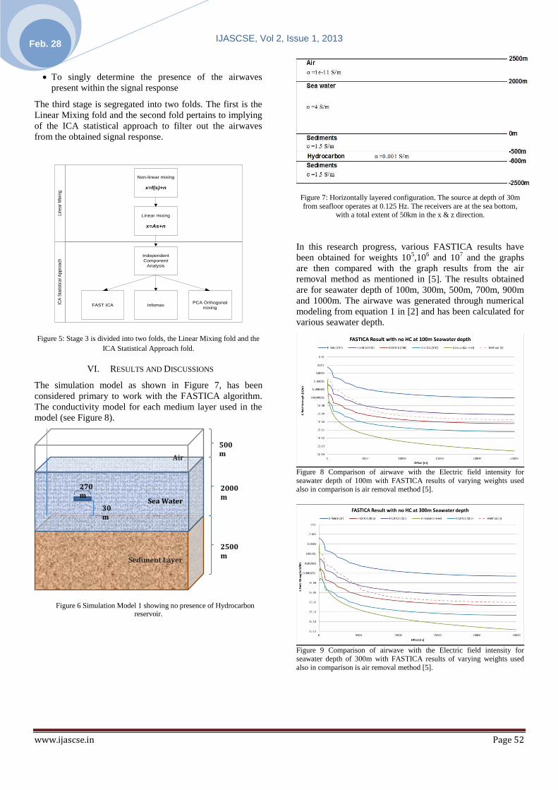
To singly determine the presence of the airwaves

present within the signal response

The third stage is segregated into two folds. The first is the

Linear Mixing fold and the second fold pertains to implying

of the ICA statistical approach to filter out the airwaves

from the obtained signal response.

Non-linear mixing

x=f(s)+n

Linear mixing

x=As+n

Independent

Component

Analysis

FAST ICA InfomaxPCA Orthogonal

mixing

Lin

ea

r M

ixin

gIC

A S

tatis

tica

l Ap

pro

ach

Figure 5: Stage 3 is divided into two folds, the Linear Mixing fold and the

ICA Statistical Approach fold.

VI. RESULTS AND DISCUSSIONS

The simulation model as shown in Figure 7, has been

considered primary to work with the FASTICA algorithm.

The conductivity model for each medium layer used in the

model (see Figure 8).

Figure 6 Simulation Model 1 showing no presence of Hydrocarbon reservoir.

Figure 7: Horizontally layered configuration. The source at depth of 30m

from seafloor operates at 0.125 Hz. The receivers are at the sea bottom, with a total extent of 50km in the x & z direction.

In this research progress, various FASTICA results have

been obtained for weights 105,10

6 and 10

7 and the graphs

are then compared with the graph results from the air

removal method as mentioned in [5]. The results obtained

are for seawater depth of 100m, 300m, 500m, 700m, 900m

and 1000m. The airwave was generated through numerical

modeling from equation 1 in [2] and has been calculated for

various seawater depth.

Figure 8 Comparison of airwave with the Electric field intensity for

seawater depth of 100m with FASTICA results of varying weights used

also in comparison is air removal method [5].

Figure 9 Comparison of airwave with the Electric field intensity for seawater depth of 300m with FASTICA results of varying weights used


500 m

2000 m

2500 m

Sediment Layer

Sea Water

270 m

30 m

Air



Feb. 28







The reason for selecting weights of range from 105 till 10

7 is

because the sample values of the E-field intensity is of very

minute values ranging from 106 till 10

15.

From Table I and from Figure 8 to 13, it is very evident that

the magnitude of the FASTICA result of weight 106 is very

close to the results from [5] for far offset from 15km till 25

km.

In shallow water setting, the EM waves reverberate more

often, resulting in higher electric field strength at the

receiver response.




Figure 13 Comparison of airwave with the Electric field intensity for seawater depth of 100m with FASTICA results of varying weights used


Table I. Comparison of magnitude of FASTICA results for varying seawater depth at Offset 25,000m of varying weights with Method of air

removal from [5].

Seawater Depth (m)

Results from FASTICA (105)



1000 643% -26% -91%

900 618% -28% -93%

700 482% -42% -94%

500 426% -47% -95%

300 353% -55% -95%

100 330% -66% -97%

This is the main reason as to why the airwaves mask the

important informative signals at far offsets. The FASTICA



Feb. 28

results for each seawater depth are at an intermittent level

between the CST simulation recordings with the calculated

airwave. The graphs of FASTICA results of varying weights

105, 10

6 and 10

7 are equidistant from each other, with the

105 weight having most E-field strength, whilst the weight

107, the E-field strength is significantly reduced, resulting in

a graph slightly closer to the actual airwave.

The airwave removal results from [5] are projected and

compared with the FASTICA results of varying weights so

as to ascertain the reliability in the results obtained from

FASTICA. Since the results from [5] coincide significantly

with the FASTICA result of weight 106 by a percentage

difference of minimum 26%, also we consider the offset

from 15km till 25km as airwaves are more imminent at a far

off distance. Hence from conclusion, we can say that the

FASTICA result of weight 106 gives better results of the

EM response without the airwaves.

VII. CONCLUSION

In conclusion, we have performed FASTICA algorithm over

the CST simulation results based over the no Hydrocarbon

simulation model by varying the weights used. The results

from the FASTICA of weights 105, 10

6 and 10

7 are

determined and compared with the air wave removal

method in [5] for validation of the results. The weight 106

coincides with the results from [5] at far offsets from 15km

till 25km. Hence weight 106 approximates the best results.

Since we have now obtained the result set from FASTICA

algorithm in deciphering out the airwaves, future work is to

commence with the other algorithms that is, PCA-

orthogonal mixing algorithm using ICA. Along with that,

we will use complex simulation modeling environments for

algorithm testing for evaluation and validation.

REFERENCES

[1] Andreis, D., L. MacGregor,” Controlled-Source Electromagnetic

Sounding in Shallow Water: Principles and applications”, Geophysics

Journal, vol. 73, pp 21-32, 2008. [2] Janniche Iren Nordskag, Lasse Amundsen,"Asymptotic airwave

modeling for marine controlled-source electromagnetic surveying",

Geophysics, Vol. 72, NO. 6, November-December 2007; P. F249–F255

[3] A. Shaw1, A.I. Al-Shamma’a, S.R. Wylie, D. Toal,"Experimental

Investigations of Electromagnetic Wave Propagation in Seawater", Proceedings of the 36th European Microwave Conference, September

2006, Manchester UK

[4] Tage Røsten, Lasse Amundsen,"Generalized electromagnetic seabed logging wavefield decomposition into U/D-going components", 2006

Society of Exploration Geophysicists, SEG Expanded Abstracts 23,

592 (2004). [5] Lars O. Løseth, Lasse Amundsen, and Arne J. K. Jenssen,“A solution

to the airwave-removal problem in shallow-water marine EM”, Geophysics,Vol. 75, No. 5 September-October 2010, P. A37–A42.

[6] H.M. Zaid, N.B. Yahya, M.N. Akhtar, M. Kashif, H. Daud, S.

Brahim, A. Shafie, N.H.H.M. Hanif, A.A.B. Zorkepli,"1D EM

Modeling for Onshore Hydrocarbon Detection using MATLAB", Journal of Applied Sciences 2011, 2011 Asian Network for Scientific

Information.

[7] Hanita Daud, Noorhana Yahya, Vijanth Asirvadam, Khairul Ihsan Talib,"Air Waves Effect on Sea Bed Logging for Shallow Water

Application", 2010 IEEE Symposium on Industrial Electronics and Applications (ISIEA 2010), October 3-5, 2010, Penang, Malaysia.

[8] Article "C.5.8 CMarine CSEM exploration", Geophysics 424 October

2008. [9] S. E. Johansen, H.E.F. Amundsen, T.Rosten, S. Ellingsrud,

T.Eidesmo, A.H. Bhuiyan, “Subsurface Hydrocarbon Detected by

Electromagnetic Sounding”, Technical Article, First Break Volume 23, March 2005.

[10] Peter Weidelt,” Guided Waves in Marine CSEM and the Adjustment

Distance in MT: A Synopsis”, Electromagnetic Colloquium, Czech Republic, Oct 1-5, 2007.

[11] Cox, C.S. Constable, S.C., Chave, A.D, Webb S.C., “Controlled

source Electromagnetic Sounding of the oceanic Lithosphere,” Nature Magazine, 1986, 320, pp 52-54.