Independent components in acoustic emission

energy signals from large diesel engines

Niels Henrik Pontoppidan1 and Sigurdur Sigurdsson2

Informatics and Mathematical ModelingRichard Petersens Plads

Technical University of Denmark Building 3212800 Lyngby Denmark

Submitted to International Journal of COMADEM

1corresponding author, nhp@imm.dtu.dk2siggi@imm.dtu.dk

Abstract

This paper analyses acoustic emission energy signals acquired under mixed load

conditions with one induced fault. With Mean field independent components

analysis is applied to an observation matrix build from successive acoustic emis-

sion energy revolution signals. The paper presents novel results that provide

remarkable automatic grouping of the observed signals equivalent to the group-

ing obtained by human experts. It is assumed that the observed signals are

a non-negative mixture of the hidden (non-observable) non-negative acoustic

energy source signals. The mean field independent component analysis incorpo-

rates those constraints and the estimates of the hidden signals are meaningful

compared to the known conditions and changes in the experiment. Most im-

portant is the estimate of the load independent wear profile due to the induced

fault. The strength of this signature increases as the load progress and disap-

pear as the induced fault is removed – this result has not been achieved with

classical independent components analysis or principal components analysis.

1 Introduction

In the last two decades blind source separation by independent components

analysis (ICA) have gained a lot of attention. ICA has been reported to sepa-

rate speakers in mixtures [1], spotting topics in chat rooms [6], finding activation

patterns in functional neuroimages [9] just to mention a few applications. Re-

cently ICA was reported to provide cognitive groupings from observed signals

without any prior knowledge of the true groupings. There Cognitive component

analysis (COCA) is defined as the process of unsupervised grouping of data such

that the ensuing group structure is well-aligned with that resulting from human

cognitive activity [4, 2]. In this paper I show how similar results can be obtained

from applying the mean field independent components analysis (MFICA) algo-

rithm, due to Højen-Sørensen et al. [5], to acoustic emission (AE) energy signals

obtained from a large diesel engine. The experiments show that the MFICA al-

gorithm is capable of extracting a signal profile describing an induced fault and

its development, which is not the case for the Information maximization ICA

[1] and Principal component analysis. In this paper no performance numbers

are given, instead the raw output of the ICA algorithms are provided as they

speak for themselves.

2 Experimental data

Acoustic emission signals were acquired from the two stroke MAN B&W test

bed engine in Copenhagen. The signals were sampled at 20 KHz after analogue

RMS filtering (τ = 120µs) had been applied. Also the Top Dead Center and

angle encoder signals were obtained, and the AE RMS signals were segmented

into single revolutions (at bottom dead center) before domain was changed to

crank angle. This results in signals with 2048 points pr. revolution as seen in

1

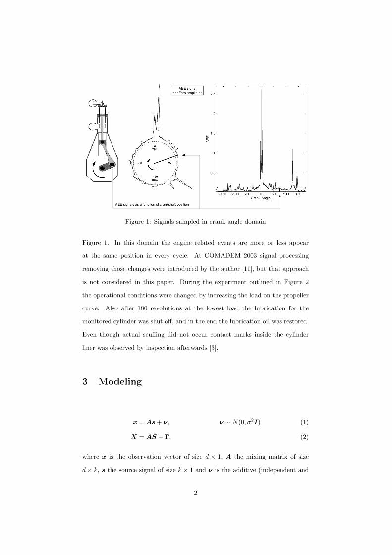
Figure 1: Signals sampled in crank angle domain

Figure 1. In this domain the engine related events are more or less appear

at the same position in every cycle. At COMADEM 2003 signal processing

removing those changes were introduced by the author [11], but that approach

is not considered in this paper. During the experiment outlined in Figure 2

the operational conditions were changed by increasing the load on the propeller

curve. Also after 180 revolutions at the lowest load the lubrication for the

monitored cylinder was shut off, and in the end the lubrication oil was restored.

Even though actual scuffing did not occur contact marks inside the cylinder

liner was observed by inspection afterwards [3].

3 Modeling

x = As + ν, ν ∼ N(0, σ2I) (1)

X = AS + Γ, (2)

where x is the observation vector of size d × 1, A the mixing matrix of size

d × k, s the source signal of size k × 1 and ν is the additive (independent and

2

Figure 2: Time line for destructive experiment carried out with MAN B&W’stest bed engine

identically distributed) i.i.d. Gaussian noise with variance σ2 also of size d× 1.

d is the number of features and k the number of components, and k � d. The

noise is assumed to be i.i.d. Gaussian even though the RMS conditioning turns

an uncorrelated zero mean additive noise component into a strictly non-negative

noise component. However such noise model is not currently available with the

MFICA algorithm. The MFICA algorithm differs from other ICA algorithms

by allowing a broad range of source priors and mixing matrix constraints. For

more information on the MFICA algorithm refer to [5] and [7].

The observation matrix X is generated by stacking several realizations of

the observation vectors. Here the different realizations come from different

engine revolutions acquired with the same sensor. Simultaneously should be

understood as at same angular position in this setup, and not as simultaneously

recorded as the case in the classical blind source separation problems [1, 8].

Similarly the source matrix S and the noise matrix Γ comes from stacking the

3

N source vectors and noise vectors.

X = {x1,x2, . . . ,xN} (3)

S = {s1, s2, . . . , sN} (4)

Γ = {ν1,ν2, . . . ,νN} (5)

Equation 1 describe how the k hidden signals in A are weighted by the co-

efficients in s to generate the observed signal x. In other words the A matrix

contain those signal parts that the observed signals can be made up from - it

acts like a basis for the normal condition. The idea is to learn this basis set from

a collection of normal condition data, making the model capable of generating

the different modes in the observed training data. By applying the component

analysis methods the orthogonal/independent directions in the observed data

should result in a basis, i.e., columns in the mixing matrix, that contains signa-

tures with the descriptive quality like source 3 (the third row of S) model the

amplitude of the injector event signal in column 3 of the mixing matrix.

In Figure 3 the modeling of a normal and a faulty example (both at 25%

load) is given. The source matrix reveals that the 2nd hidden signal models

the normal condition part, while the 1st hidden signal models the additional

part arising from the fault condition. However the two hidden signals are quite

similar. The mixing matrix with the independent directions was estimated

from 25% normal and faulty examples. We will later see much more difference

between the hidden signals when two additional loads

3.1 Principal Components Analysis

The Principal components are obtained from the Singular Value Decomposition

of the observation matrix X = UDV >. The 4 component mixing matrix is

4

Figure 3: Data matrix setup. The first example is normal and the second faulty.The mixing matrix was obtained from observations at 25% load only

estimated as the four first columns of the left hand side matrix U . The four

source components are estimated as four first columns of the left hand side

matrix V weighted by the four largest singular values (and transposed). The

method and matrix setup is further described in [10].

3.2 Information maximization ICA

The Information maximization ICA (IMICA) due to [1] require that the mixing

matrix is A square as the source estimates are obtained from S = A−1X. This

implies that the number of sources and observations should be equal, in this

case 2227 sources! Often PCA is used reduce the dimensionality, such that

S = A−1UX so actually the input to the IMICA is the 4 principal components

shown in Figure 7. The method and matrix setup is further described in [10].

5

Figure 4: The full data set. The amplitude is color coded, i.e., the stronger thesignal the darker the color.

Figure 5: The independent components. Source 1 models the increased weardue to the removed oil. Source 2, 3, and 4 model the 25%, 50% and 75%load respectively. Changes in the source signals comply with the occurrence ofoperational changes given in Figure 2

6

Figure 6: The hidden signals (columns of the mixing matrix A). The first onepicks up the increased friction profile while the remaining model the normalcondition at 25%, 50% and 75% load

4 Finding the increased wear signature

Now we consider the full data set shown in Figure 4 and apply the MFICA

algorithm to estimate the hidden signals and the independent activations of

those hidden signals. The only knowledge that the algorithm is given is that it is

non-negative mixing of four independent non-negative sources. No information

is given on the operational changes and the induced faulty - thus the separation

is unsupervised.

The results in Figure 5 are impressive: Source 1 model the wear due to

increased friction between piston and liner. It suddenly appears just after the

oil was shut down, increases throughout the experiment until the lube oil system

is restored. The remaining sources model the load changes, with only slight

problems of separating the 50% and 75% loads fully. It is fair to conclude that

the MFICA resulted in a highly informative clustering of the observed signals,

directly in line how we group the observations, and thus an example of the

7

powerful cognitive properties of the independent components as reported in [4].

Also the hidden signals shown in Figure 5 are remarkable. The first signal

clearly picks up the more or less constant noise from the increased friction; it is

lower in the beginning and in the end possibly due to the fact that the cylinder

sucked up oil from the outer cylinders from the bottom tub. The signal also

contains the quite severe component that is generated when the piston passes

the scavenge air holes in the downstroke. The remaining components model

the changes in the normal condition signals as a function of the load, e.g., the

movement of the peaks in the injection period right after TDC. The hidden

signals shown in Figure 3 were obtained from normal and faulty examples at

25% load. When comparing those to the ones obtained with the additional

examples from 50% and 75% load, the MFICA algorithm was able to provide a

much better estimate of the signal component modeling the increased friction

between piston and liner. With the multiple loads the independence of the

increased friction signal and the normal engine events become more apparent

for the algorithm.

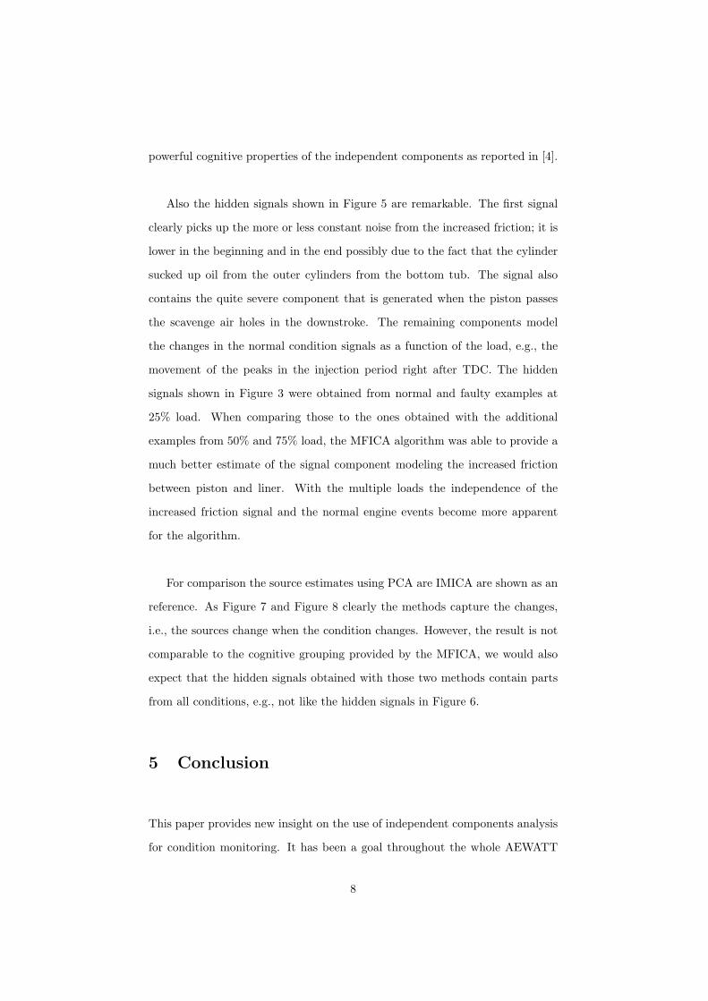
For comparison the source estimates using PCA are IMICA are shown as an

reference. As Figure 7 and Figure 8 clearly the methods capture the changes,

i.e., the sources change when the condition changes. However, the result is not

comparable to the cognitive grouping provided by the MFICA, we would also

expect that the hidden signals obtained with those two methods contain parts

from all conditions, e.g., not like the hidden signals in Figure 6.

5 Conclusion

This paper provides new insight on the use of independent components analysis

for condition monitoring. It has been a goal throughout the whole AEWATT

8

project to find a signal component that picks up the increased friction between

piston and liner regardless of the operational condition. The accurate grouping

of the examples obtained without telling the algorithm what to look for was

remarkable and fully aligned with the experimental setup. We believe that this

this provides new and promising opportunities in field of condition monitoring.

Acknowledgements

The European Commission is acknowledged for the funding of this work through

the 5th framework AEWATT project. Experimental data was generously pro-

vided by project partners at MAN B&W. The engine sketch in Figure 1 is due to

Ryan Douglas, Heriot-Watt University. The presentation and discussion on cog-

nitive components in our local journal club provided inspiration for this work.

Figure 7: Source estimates using principal components analysis of the wholedata set.

References

[1] A. Bell and T. Sejnowski. An information-maximisation approach to blind

separation and blind deconvolution. Neural Computation, 7(6):1129–1159,

9

Figure 8: Source estimates using Information maximization ICA on the wholedata set.

1995.

[2] L. Feng, L. K. Hansen, and J. Larsen. On low level cognitive components

of speech. In Honkela et al., editor, AKKR’05 International and Interdisci-

plinary Conference on Adaptive Knowledge Representation and Reasoning,

Helsinki, Finland, jun 2005. Pattern Recognition Society of Finland.

[3] Torben Fog. Scuffing Experiment, Experiment Log. 2000.

[4] L. K. Hansen, P. Ahrendt, and J. Larsen. Towards cognitive component

analysis. In Finnish Cognitive Linguistics Society Pattern Recognition So-

ciety of Finland, Finnish Artificial Intelligence Society, editor, AKRR’05

-International and Interdisciplinary Conference on Adaptive Knowledge

Representation and Reasoning. Pattern Recognition Society of Finland,

Finnish Artificial Intelligence Society, Finnish Cognitive Linguistics Soci-

ety, jun 2005.

[5] P. A. Højen-Sørensen, O. Winther, and L. K. Hansen. Mean field ap-

proaches to independent component analysis. Neural Computation, 14:889–

918, 2002.

[6] T. Kolenda, L. K. Hansen, and S. Sigurdsson. Indepedent components

in text. In Advances in Independent Component Analysis, pages 229–250.

Springer-Verlag, 2000.

10

[7] T. Kolenda, S. Sigurdsson, O. Winther, L. K. Hansen, and J. Larsen.

DTU:Toolbox. Internet, 2002. http://isp.imm.dtu.dk/toolbox/.

[8] L. Molgedey and H.G. Schuster. Separation of a mixture of independent

signals using time delayed correlations. Phys. Rev. Lett., 72(23):3634–3637,

1994.

[9] K. Petersen, L. K. Hansen, T. Kolenda, and E. Rostrup. On the indepen-

dent components of functional neuroimages. In Third International Con-

ference on Independent Component Analysis and Blind Source Separation,

pages 615–620, 2000.

[10] N. H. Pontoppidan, J. Larsen, and T. Fog. Independent component analy-

sis for detection of condition changes in large diesels. In Om P. Shrivastav,

Bassim Al-Najjar, and Raj B.K.N. Rao, editors, COMADEM 2003. CO-

MADEM International, 2003.

[11] Niels Henrik Pontoppidan and Ryan Douglas. Event alignment, warping

between running speeds. In Raj B.K.N. Rao, Barry E. Jones, and Roger I.

Grosvenor, editors, COMADEM 2004, pages 621–628, Birmingham, UK,

aug 2004. COMADEM International.

11