independent sets and graph coloring with applications to the frequency allocation problem in...
TRANSCRIPT
Independent Sets and Graph Coloring with Applications to the Frequency Allocation Problem in
Wireless Networks
Evi Papaioannou
PhD Thesis
Department of Computer Engineering and InformaticsUniversity of Patras

Subject
• Wireless networks
– Frequency allocation problem in cellular wireless netowrks
– Call control problem in wireless networks with cellular, planar, arbitrary topology
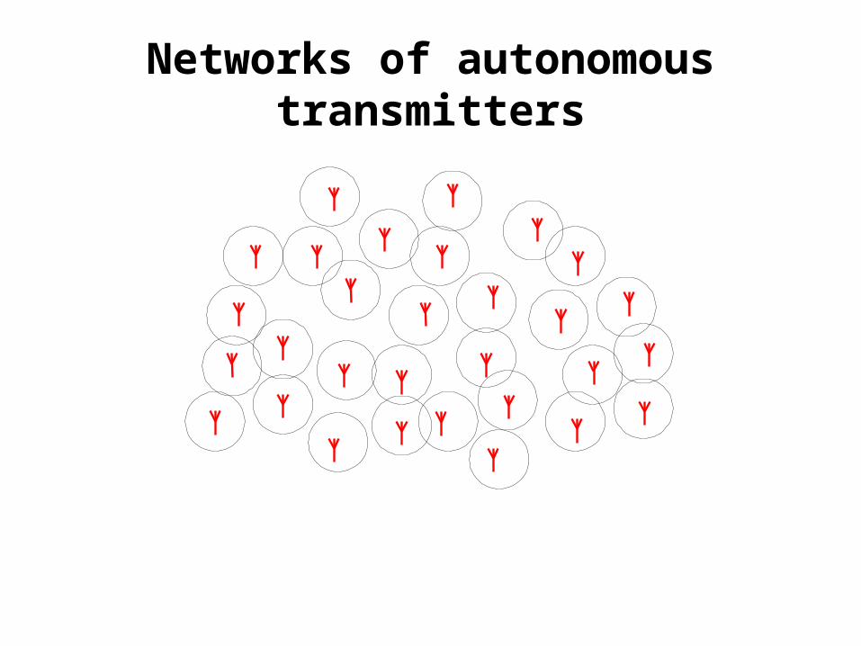
• Networks of autonomous transmitters
– Maximum independent set problem
– Minimum coloring problem

Methodology
• On-line problems– Users/transmitters appear gradually and the
sequence can stop arbitrarily
– On-line algorithms
– Algorithms cannot change their choices
• Performance evaluation – Competitive analysis
– Metric = value of competitive ratio

Cellular wireless networks
• The geographical area is divided in regions (cells)• Each cell is the calling area of a base station• Base stations are interconnected via a high speed
network

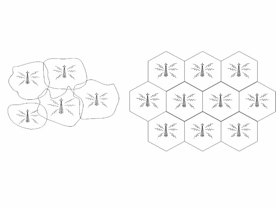

Communication
• Communication between user and base station is always required
• Frequency Division Multiplexing (FDM) Technology : many users within the same cell can simultaneously communicate with their base station using different frequencies [Hale 80]
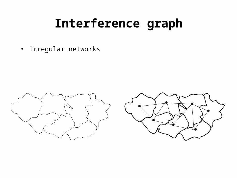
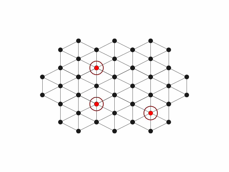
Interference graph
• Irregular networks

Interference graph
• Cellular networks– Reuse distance (k): the min distance between two cells
where the same frequency can be used

Frequency allocation
Input• A cellular network and users that wish to communicate
with their base station
Output• Frequency allocation to all users, so that:
– Users in the same or adjacent cells are assigned distinct frequencies
– The number of frequencies used in minimized

Graph coloring
Imagine:• Frequencies colors• Users that wish to communicate with their base station
nodes of the interference graph of the wireless network
Then:• Frequency allocation problem problem of
multicoloring the nodes of the interference graph• The interference graph is constructed gradually
– Nodes are added gradually as calls appear

Call control
Input• A cellular network supporting w frequencies and users
that wish to communicate with their base station
Output• Frequency allocation to some of the users, so that:
– Users in the same or adjacent cells are assigned distinct frequencies
– At most w frequencies are used– The number of the users served is maximized
Independent sets
Imagine:• Frequencies colors• Users that wish to communicate with their base station
nodes of the interference graph of the wireless network
Then:• Call control problem Maximum independent set
problem in the interference graph• The interference graph is constructed gradually
– Nodes are added gradually as calls appear

Competitive analysis
Frequency allocationCost:• Number of frequencies used
Competitive ratio:
Call ControlBenefit:• Number of users served
Competitive ratio:
) σ (C) σ (C
maxρOPT
A
σ
) σ (C)] σ (E[C
maxρOPT
A
σ
) σ (B) σ (B
maxρA
OPT
σ
)] σ (E[B) σ (B
maxρA
OPT
σ

Frequency allocation
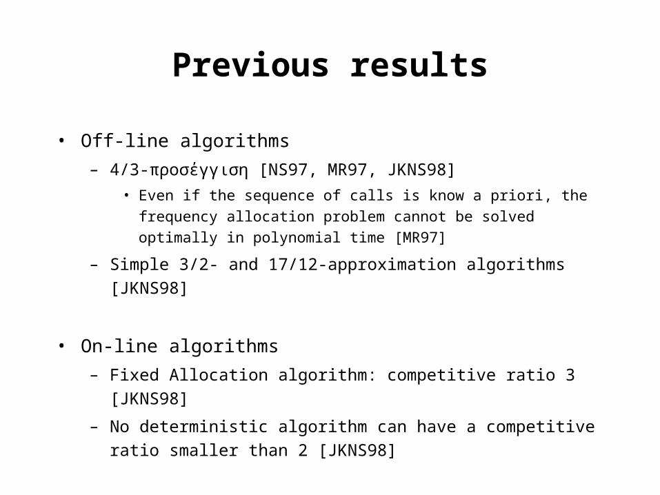
Previous results
• Off-line algorithms
– 4/3-προσέγγιση [NS97, MR97, JKNS98]
• Even if the sequence of calls is know a priori, the frequency allocation problem cannot be solved optimally in polynomial time [MR97]
– Simple 3/2- and 17/12-approximation algorithms [JKNS98]
• On-line algorithms
– Fixed Allocation algorithm: competitive ratio 3 [JKNS98]
– No deterministic algorithm can have a competitive ratio smaller than 2 [JKNS98]


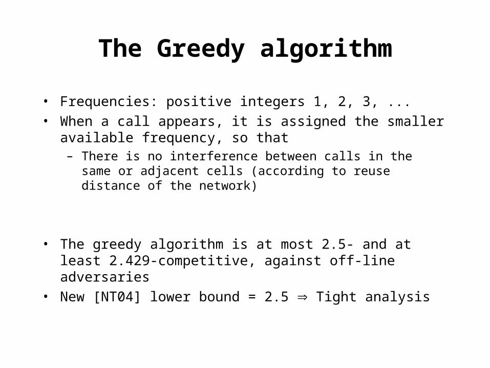
The Greedy algorithm
• Frequencies: positive integers 1, 2, 3, ...• When a call appears, it is assigned the smaller available
frequency, so that– There is no interference between calls in the same or
adjacent cells (according to reuse distance of the network)
• The greedy algorithm is at most 2.5- and at least 2.429-competitive, against off-line adversaries
• New [ΝΤ04] lower bound = 2.5 Tight analysis

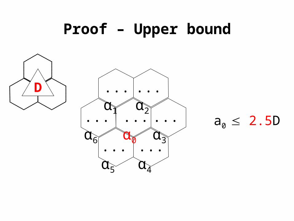
Proof – Upper bound

Proof – Upper bound
D

Proof – Upper bound
...α0
...α1
...α2
...α3...α
4
...α5
...α6
D
Proof – Upper bound
...α0
...α1
...α2
...α3...α
4
...α5
...α6
D
a0 2.5D

Proof – Lower bound

Call control

Previous results
• Greedy algorithm, networks of maximum degree Δ that support one frequency [PPS97]
Greedy algorithm
Benefit = 1
...
Optimal algorithm
......
Benefit = Δ

Previous results
• «Classify and Randomly Select» paradigm for networks with chromatic number χ that support one frequency [ΑΑFLR96, PPS97]

Previous results
• «Classify and Randomly Select» paradigm for networks with chromatic number χ that support one frequency [ΑΑFLR96, PPS97]
Chromatic number = 4
4 times worse
...
Networks of max degree ΔChromatic number Δ+1 Δ+1 times worse

Previous results
• Lower bounds for arbitrary networks [BFL96]• Simple way of transforming an algorithm designed for
networks that support one frequency to an algorithm for networks that support arbitrarily many frequencies [AAFLR01]
• Upper bounds for networks with planar and arbitrary interference graphs using the «Classify and Randomly Select» paradigm [PPS02]

The Greedy algorithm
• The greedy algorithm in networks that support one frequency achieves a competitive ratio equal to the size of the maximum independent set of every node of the interference graph
...

Deterministic algorithms
• The greedy algorithm in cellular networks that support one frequency
• Optimal in the class of deterministic on-line algorithms• Competitive ratio: 3
Benefit = 1 Benefit = 3

Randomized algorithms
• Based on the «Classify and Randomly Select» paradigm• Competitive ratio = number of colors used for the
coloring of the interference graph• Competitive ratio for cellular networks: 3

Idea
Accept the call with probability p

(1-p)t0: w.h.p. one of the calls is accepted
Marking TechniqueIdea
Accept the call with probability p

Marking TechniqueIdea
Accept the call with probability p
(1-p)t0: w.h.p. one of the calls is accepted

Algorithm p-Random
• Initially all cells are unmarked
• For each new call c in a cell v
– If v is marked, reject c
– If there is an accepted call in cell v or in its adjacent cells, reject c
– Otherwise:
• With probability p, accept c
• With probability 1-p, reject c and mark cell v

Upper bounds
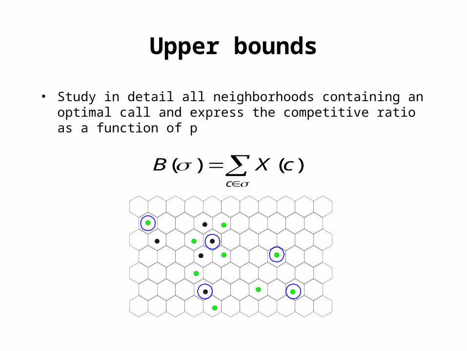
• Study in detail all neighborhoods containing an optimal call and express the competitive ratio as a function of p

Upper bounds
• Study in detail all neighborhoods containing an optimal call and express the competitive ratio as a function of p

Upper bounds
• Study in detail all neighborhoods containing an optimal call and express the competitive ratio as a function of p
Upper bounds
c
cXB )()(
• Study in detail all neighborhoods containing an optimal call and express the competitive ratio as a function of p

Upper bounds
)(')()(
))'(
)'()(()()(
ccAcAc cd
cXccbB
• Study in detail all neighborhoods containing an optimal call and express the competitive ratio as a function of p

Upper bounds
• Best upper bound: 2.651
• Study in detail all neighborhoods containing an optimal call and express the competitive ratio as a function of p

Upper bounds
• Algorithm p-Random achieves better competitive ratio than all deterministic algorithms in all networks that support one frequency– 27/28 Δ– Extend the analysis for sparse networks of degree 3 or 4
• Disadvantages– No improvement fro networks that support arbitrarily many
frequencies– Uses randomness proportional to the size of sequence of
calls

CRS-based algorithms
Objective • Randomized algorithms
• Arbitrarily many frequencies• Whatever reuse distance • Few randomness
• Weak random sources• Constant number of random bits
Given• «Classify and Randomly Select» paradigm
• Simple• Use randomness only once at the beginning• Behaves «well» independently of the number of supported
frequencies

Algorithm CRS-A
• Color the interference graph with 4 colors 0,1,2,3• Select one of the colors, ignore calls in cells colored with the
selected color and execute the greedy algorithm for all other calls
0 1 0 1 0 1 0 1 0 1
1 0 1 0 1 0 1 0 1 0
0 1 0 1 0 1 0 1 0 1
1 0 1 0 1 0 1 0 1 0
2 3 2 3 2 3 2 3 2
3 2 3 2 3 2 3 2 3
2 3 2 3 2 3 2 3 2

Algorithm CRS-A
0 1 0 1 0 1 0 1 0 1
1 0 1 0 1 0 1 0 1 0
0 1 0 1 0 1 0 1 0 1
1 0 1 0 1 0 1 0 1 0
2 3 2 3 2 3 2 3 2
3 2 3 2 3 2 3 2 3
2 3 2 3 2 3 2 3 2
3 3 3 3
3 3 3 3 3
3 3 3 3
• Color the interference graph with 4 colors 0,1,2,3• Select one of the colors, ignore calls in cells colored with the
selected color and execute the greedy algorithm for all other calls

Algorithm CRS-A: analysis
• The greedy algorithm will accept at least half of the optimal calls• Work on average on the 3/4 of the total calls• Competitive ratio = 8/3
1 0 1 1 0 1
2 2 2 22
1 0 1 1 0 1 1 0
0 0 0 1
0 0
1 0 1 1 0 1
2 2 2 22
1 0 1 1 0 1 1 0
0 0 0 1
0 0
2 2 22

CRS-based algorithms
• Network that supports w frequencies• CRS-based algorithms:
– Color the interference graph– Define v color classes from the colors used– Select equiprobably one out of v color classes– Execute the greedy algorithm only for cells colored with
colors from the selected color class
• If: – Each color belongs to at least λ different color classes, and– Each connected component of the subgraph of G
containing nodes colored with colors of the same color class is a clique
then, the CRS-based algorithm is v/λ-competitive against oblivious adversaries

Algorithm CRS-B
• Use 5 colors 0,1,2,3,4 for coloring the interference graph and define 5 color classes {0,1}, {1,2}, {2,3}, {3,4}, {4,0}
• The coloring and the color classes meet the conditions of the previous Lemma for v=5 and λ=2
• Competitive ratio = 5/2
0 1 2 43 4 0 1 2 3
0 1 2 3 4 0 1 2 3 4
0 1 2 3 4 0 1 2 3 4
0 1 2 3 4 0 1 2 3 4
3 4 0 10 1 2 3 4
3 4 0 10 1 2 3 4
3 4 0 10 1 2 3 4
Algorithm CRS-C
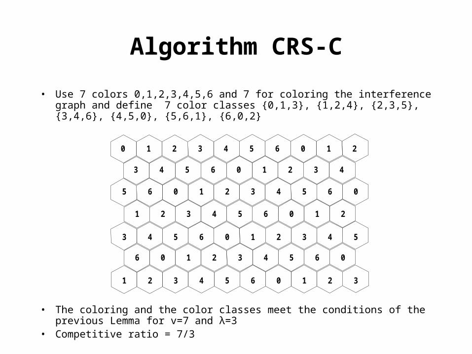
• Use 7 colors 0,1,2,3,4,5,6 and 7 for coloring the interference graph and define 7 color classes {0,1,3}, {1,2,4}, {2,3,5}, {3,4,6}, {4,5,0}, {5,6,1}, {6,0,2}
• The coloring and the color classes meet the conditions of the previous Lemma for v=7 and λ=3
• Competitive ratio = 7/3
0 1 2 13 4 5 26 0
5 6 0 61 2 3 04 5
3 4 5 46 0 1 52 3
1 2 3 24 5 6 30 1
6 0 13 4 5 2 3 4
2 3 46 0 1 5 6 0
4 5 61 2 3 0 1 2
Use of random bits
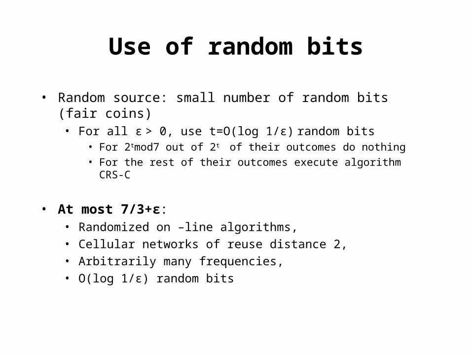
• Random source: small number of random bits (fair coins)• For all ε > 0, use t=O(log 1/ε) random bits
• For 2tmod7 out of 2t of their outcomes do nothing• For the rest of their outcomes execute algorithm CRS-C
• At most 7/3+ε: • Randomized on –line algorithms, • Cellular networks of reuse distance 2, • Arbitrarily many frequencies, • O(log 1/ε) random bits

Algorithm CRS-k
• Use λ=3k2-3k+1 colors 0,1,… 3k2-3k and 3k2-3k+1 for coloring the interference graph and define color classes appropriately so that each color belongs to– v=3k2/4 color classes, if k even– v=(3k2+1)/4 color classes, if k odd
if k even
if k odd
• Algorithms with slightly worse competitive ratios for arbitrarily many frequencies using O(log 1/ε+log k) random bits
23k13k
14CR
13k3k
14CR 2

12 16 17 1814 1513 0 1 2 3 4 5 7 8 9 106
16 17 1814 15130 1 2 3 4 5 7 8 9 10 11 126
16 17 1814 15135 7 8 9 10 11 126 0 1 2 34
16 17 18 14130 1 2 3 4 5 7 8 9 10 11 126
5 6 73 429 10 11 12 13 15 16 17 18 0 1148
1
13
6
18
11
4
16 17 1814 15132 3 4 5 7 8 9 10 11 126
14 1512 13110 1 2 3 5 6 7 8 9 104
7 16 1714 15138 9 10 11 12
5 14 1512 13116 7 8 9 10
1614 1512 13
1816 1714 15 0 1 2 3 4 5 6 7
17 18 0 1 2 3 4 5
1 2 3
5
9 10
16 17
12
18
6 7
16 17 18 0
8 9 10 11
0 1 2 3

0 1 2 3 4 5 7 8 16 17 189 10 11 126 14 1513
654321036353433323130292827
333231302928272625242322212019181716 34
23222120191817161514131211109876
7
3332 34 3635 10987654321 131211
22
12
21
2827
17
76
33 34 3635 10987654321 131211
232221201918171615141312111098 24
2322
12
141312111098765432
3332313029282726252423 34 3635 210
11 151413 2928272625242322212019181716
1514131211109876543 181716
3332313029 34 3635 87654321
33323130292827262524232221201918 34
1 1918171615
151413 28272625242322212019181716 29
33323130292827262524 34 3635 3210
0
0
0
Lower bounds
• Using Minimax Principle for randomized algorithms– k = 2, 3, 4: competitive ratio 1,857 planar network: competitive ratio 2,086– k 5: competitive ratio 25/12– k 12: competitive ratio 127/60

Networks of autonomous transmitters

Networks of autonomous transmitters
Networks of autonomous transmitters

Networks of autonomous transmitters

Networks of autonomous transmitters

Networks of autonomous transmitters

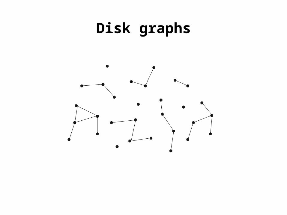
Disk graphs

Disk graphs

Disk graphs
Disk graphs

Disk graphs
Unit disk graphs

Disk graphs
σ-bounded disk graphsUnit disk graphs

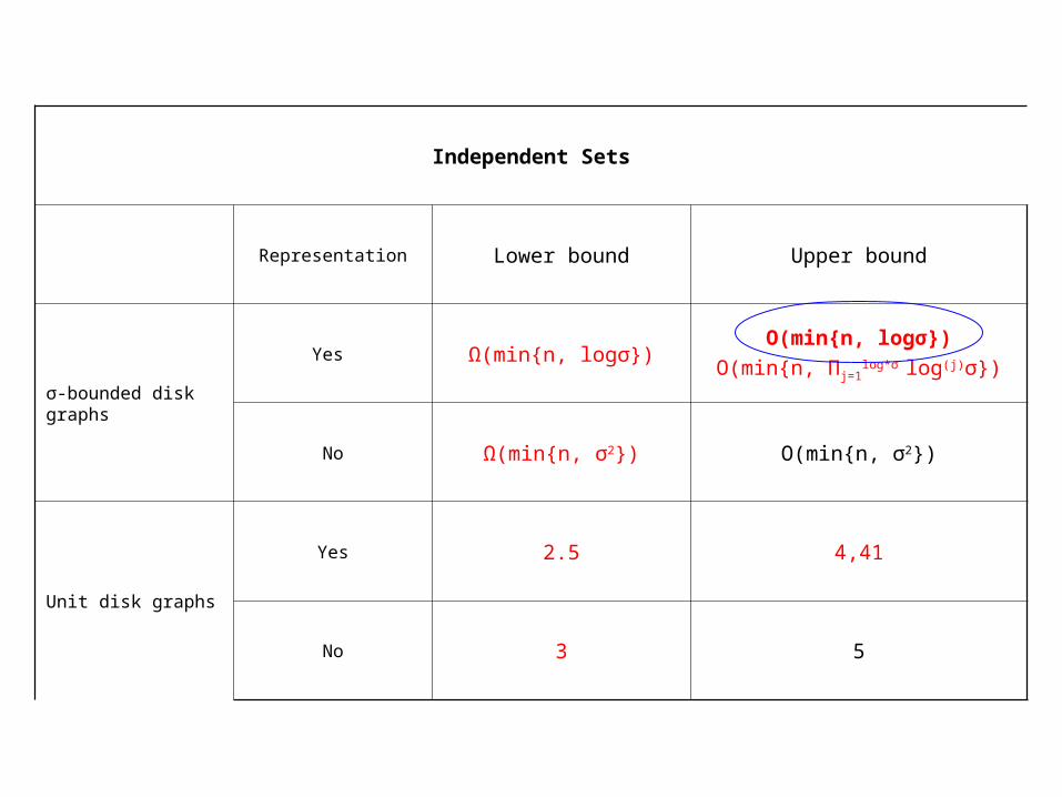
Independent Sets
Representation Lower bound Upper bound
σ-bounded disk graphs
Yes Ω(min{n, logσ})O(min{n, logσ})
O(min{n, Πj=1log*σ log(j)σ})
No Ω(min{n, σ2}) O(min{n, σ2})
Unit disk graphs
Yes 2.5 4,41
No 3 5
Independent Sets
Representation Lower bound Upper bound
σ-bounded disk graphs
Yes Ω(min{n, logσ})O(min{n, logσ})
O(min{n, Πj=1log*σ log(j)σ})
No Ω(min{n, σ2}) O(min{n, σ2})
Unit disk graphs
Yes 2.5 4,41
No 3 5
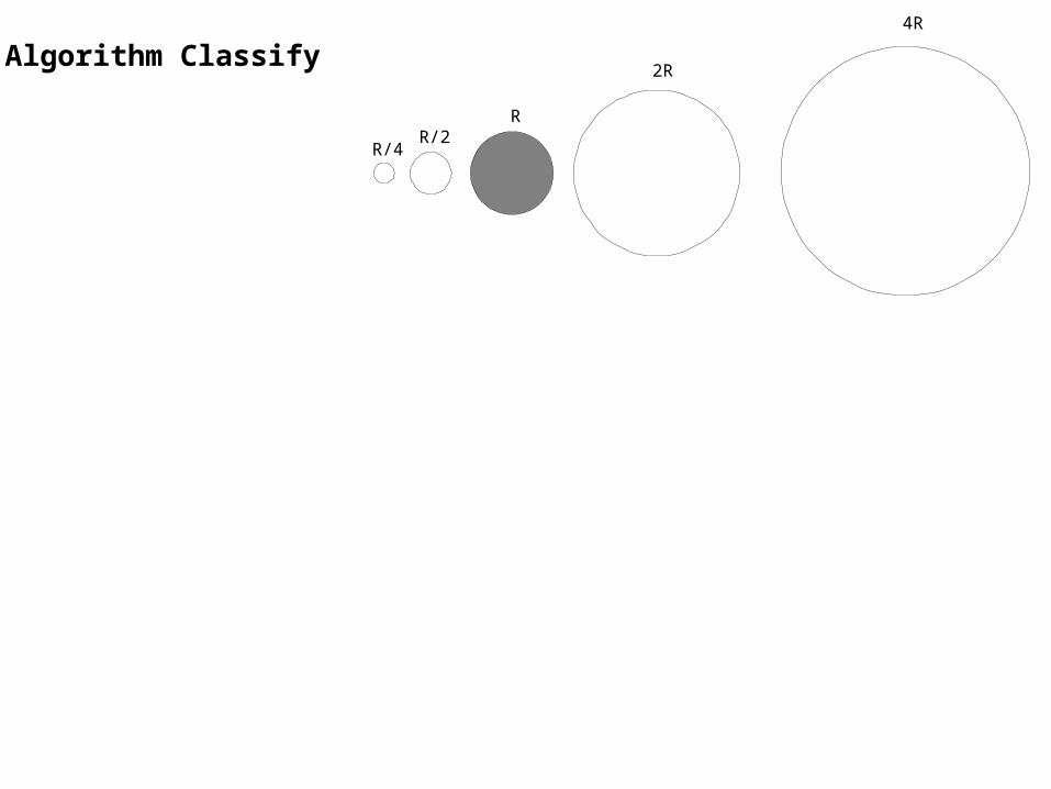
R/4R/2
R
2R
4R
Algorithm Classify

R/4R/2
R
2R
4R
Algorithm Classify

R/4R/2
R
2R
4R
Algorithm Classify
R/4R/2
R
2R
4R

R/4R/2
R
2R
4R
Algorithm Classify
R/4R/2
R
2R
4R

R/4R/2
R
2R
4R
Algorithm Classify
R/4R/2
R
2R
4R

2
1
σ = 2
24
2
3
1 7
9
8
6
1011
12
13
14
155
R/4R/2
R
2R
4R
Algorithm Classify
R/4R/2
R
2R
4R

Independent Sets
Representation Lower bound Upper bound
σ-bounded disk graphs
Yes Ω(min{n, logσ})O(min{n, logσ})
O(min{n, Πj=1log*σ log(j)σ})
No Ω(min{n, σ2}) O(min{n, σ2})
Unit disk graphs
Yes 2.5 4,41
No 3 5
R/4R/2
R
2R
4R
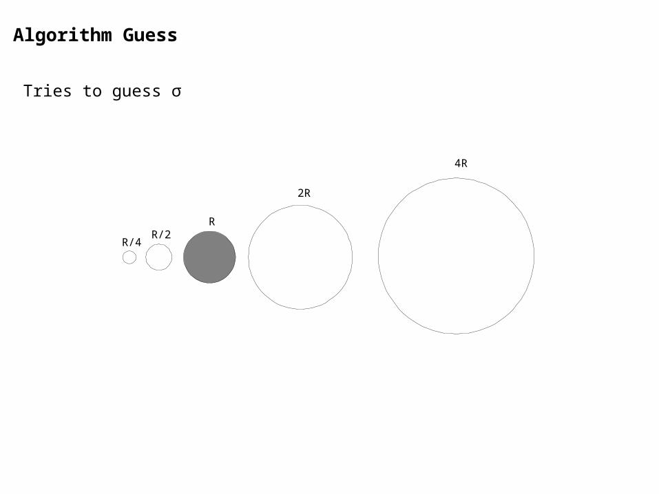
Algorithm Guess
Tries to guess σ

R/4R/2
R
2R
4R
Algorithm Guess
Tries to guess σ

R/4R/2
R
2R
4R
Algorithm Guess
Tries to guess σ

Independent Sets
Representation Lower bound Upper bound
σ-bounded disk graphs
Yes Ω(min{n, logσ})O(min{n, logσ})
O(min{n, Πj=1log*σ log(j)σ})
No Ω(min{n, σ2}) O(min{n, σ2})
Unit disk graphs
Yes 2.5 4,41
No 3 5

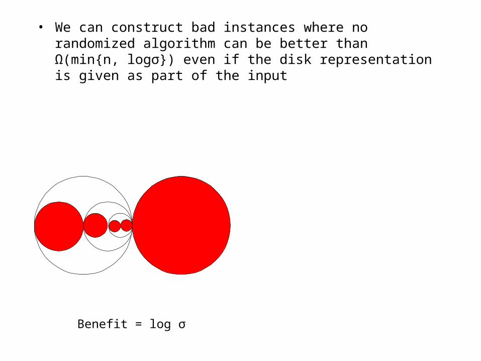
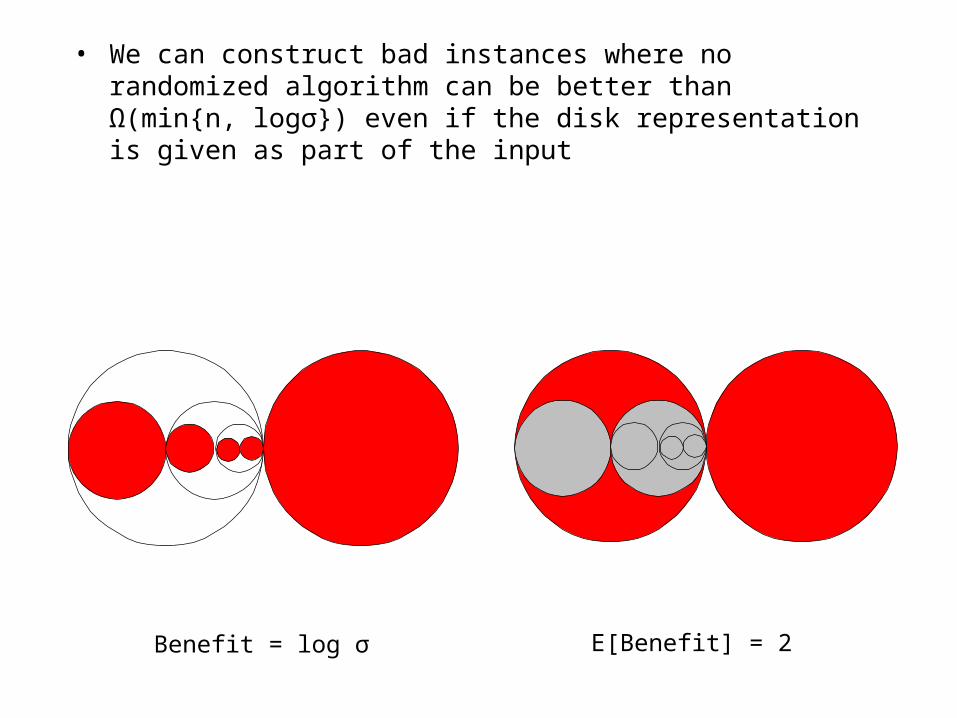
• We can construct bad instances where no randomized algorithm can be better than Ω(min{n, logσ}) even if the disk representation is given as part of the input

• We can construct bad instances where no randomized algorithm can be better than Ω(min{n, logσ}) even if the disk representation is given as part of the input

• We can construct bad instances where no randomized algorithm can be better than Ω(min{n, logσ}) even if the disk representation is given as part of the input

• We can construct bad instances where no randomized algorithm can be better than Ω(min{n, logσ}) even if the disk representation is given as part of the input

• We can construct bad instances where no randomized algorithm can be better than Ω(min{n, logσ}) even if the disk representation is given as part of the input
• We can construct bad instances where no randomized algorithm can be better than Ω(min{n, logσ}) even if the disk representation is given as part of the input
Benefit = log σ
• We can construct bad instances where no randomized algorithm can be better than Ω(min{n, logσ}) even if the disk representation is given as part of the input
Benefit = log σ Ε[Benefit] = 2

Independent Sets
Representation Lower bound Upper bound
σ-bounded disk graphs
Yes Ω(min{n, logσ})O(min{n, logσ})
O(min{n, Πj=1log*σ log(j)σ})
No Ω(min{n, σ2}) O(min{n, σ2})
Unit disk graphs
Yes 2.5 4,41
No 3 5
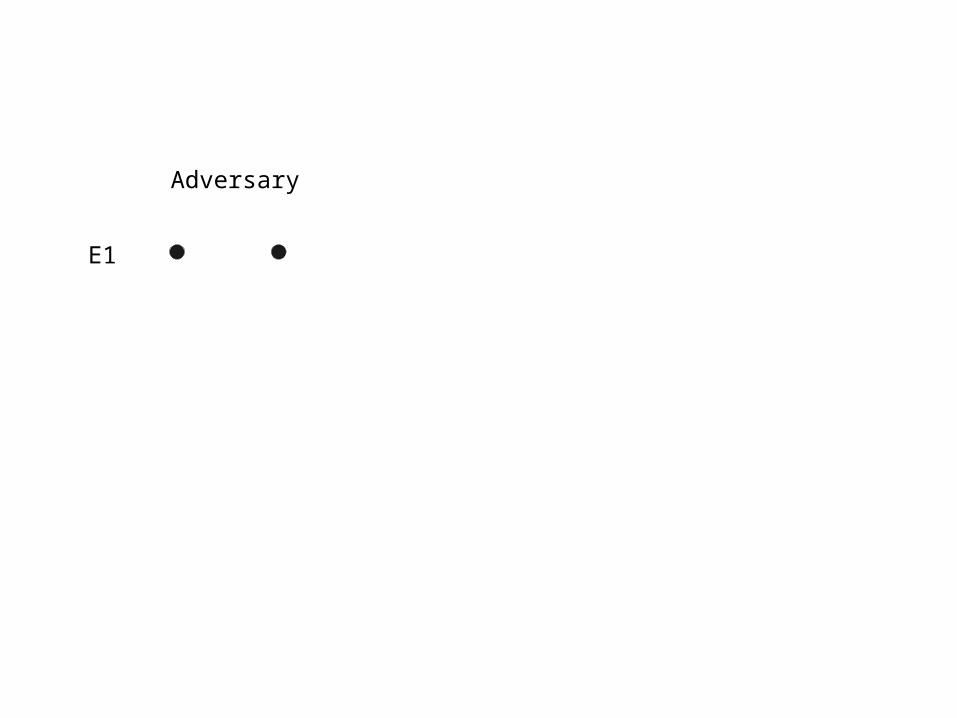
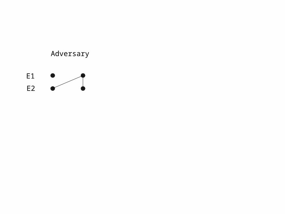
Adversary
Ε1
Adversary
Ε1
Ε2

Adversary
Ε1
Ε2
Ε3

Adversary
Ε1
Ε2
Ε3
Εκ-1
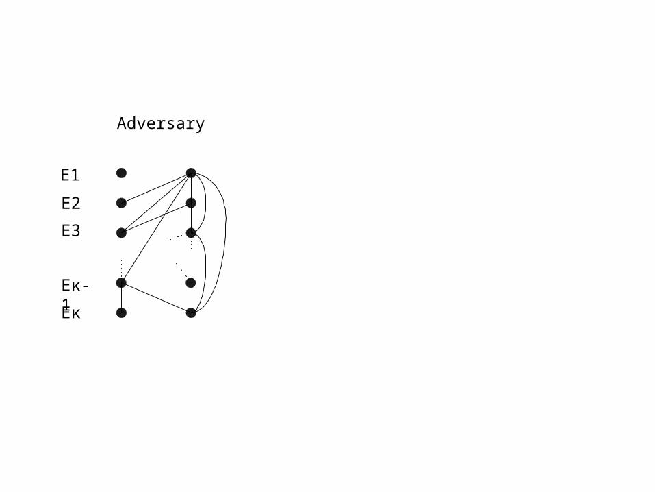
Adversary
Ε1
Ε2
Ε3
Εκ-1
Εκ
OptimalAlgorithm
Benefit = κ+1
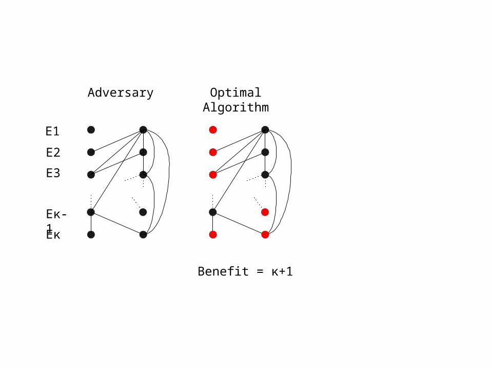
Adversary
Ε1
Ε2
Ε3
Εκ-1
Εκ

Optimal Algorithm
Benefit = κ+1
Adversary
Ε1
Ε2
Ε3
Εκ-1
Εκ
Randomized Algorithm
Ε[Benefit] 2


Disk graph for κ=Ω(min{n, σ2})

Independent Sets
Representation Lower bound Upper bound
σ-bounded disk graphs
Yes Ω(min{n, logσ})O(min{n, logσ})
O(min{n, Πj=1log*σ log(j)σ})
No Ω(min{n, σ2}) O(min{n, σ2})
Unit disk graphs
Yes 2.5 4,41
No 3 5

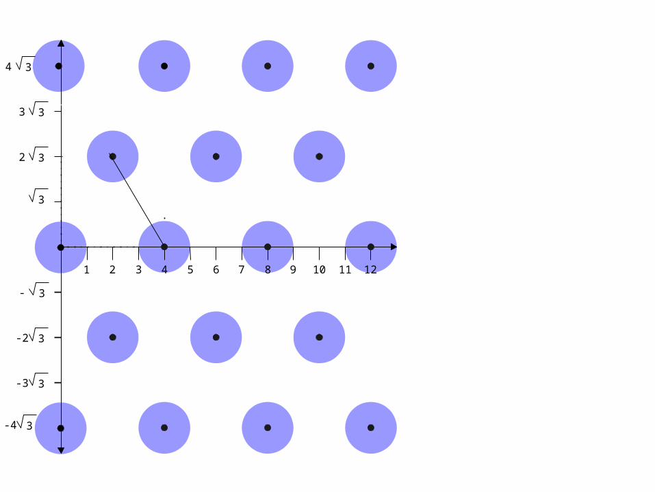
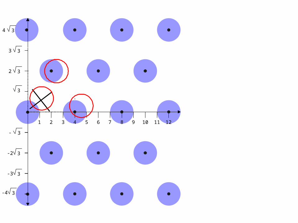
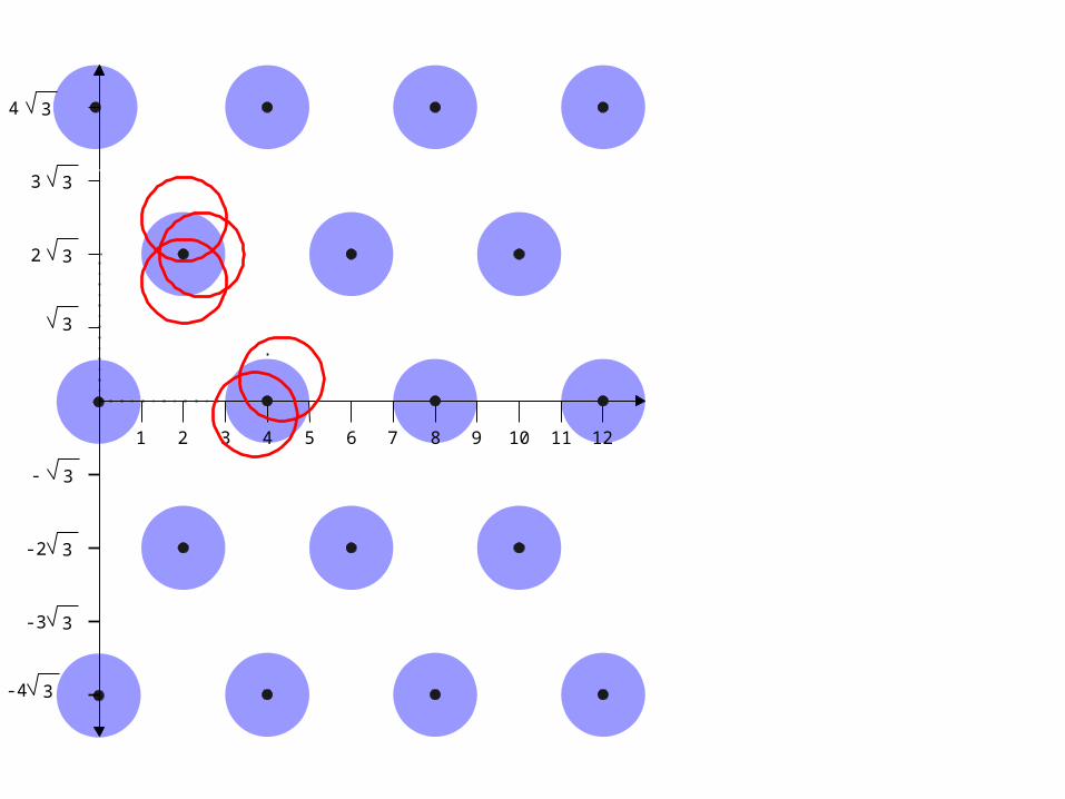
Algorithm Filter
• IDEA: – Use a 2-dimensional geometric construction, place it
uniformly at random on the plane and work only on disks from specific parts of it
(x,y)(x’,y’)
32
4

1 2 3 4 5 6 7 8 9 10 11 12
3
34
33
32
3-
3-2
3-3
3-4
1 2 3 4 5 6 7 8 9 10 11 12
3
34
33
32
3-
3-2
3-3
3-4

1 2 3 4 5 6 7 8 9 10 11 12
3
34
33
32
3-
3-2
3-3
3-4
Ο
C
A
B
1 2 3 4 5 6 7 8 9 10 11 12
3
34
33
32
3-
3-2
3-3
3-4
1 2 3 4 5 6 7 8 9 10 11 12
3
34
33
32
3-
3-2
3-3
3-4

1 2 3 4 5 6 7 8 9 10 11 12
3
34
33
32
3-
3-2
3-3
3-4

1 2 3 4 5 6 7 8 9 10 11 12
3
34
33
32
3-
3-2
3-3
3-4

1 2 3 4 5 6 7 8 9 10 11 12
3
34
33
32
3-
3-2
3-3
3-4

1 2 3 4 5 6 7 8 9 10 11 12
3
34
33
32
3-
3-2
3-3
3-4
π 12
4x23
4.41
1

Independent Sets
Representation Lower bound Upper bound
σ-bounded disk graphs
Yes Ω(min{n, logσ})O(min{n, logσ})
O(min{n, Πj=1log*σ log(j)σ})
No Ω(min{n, σ2}) O(min{n, σ2})
Unit disk graphs
Yes 2.5 4,41
No 3 5

1
2
3
4
5
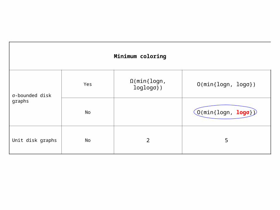
Minimum coloring
σ-bounded disk graphs
Yes Ω(min{logn, loglogσ}) O(min{logn, logσ})
No O(min{logn, logσ})
Unit disk graphs No 2 5

Algorithm Layered
At most logσ+1 layers
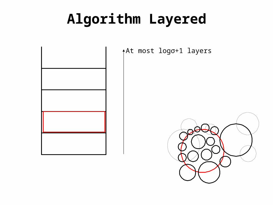
Algorithm Layered
At most logσ+1 layers

First Fit Layered
Combination of Layered and First Fit
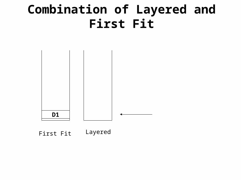
First Fit Layered
D1
Combination of Layered and First Fit

First Fit Layered
D1 d1
Combination of Layered and First Fit

First Fit Layered
D1 d1
Didi-1
Combination of Layered and First Fit

First Fit Layered
D1 d1
Didi-1
logn OPT logσ OPT
Combination of Layered and First Fit

Open problems
• Close the gap between upper and lower bounds– Call control in cellular networks– Maximum independent set problem on unit disk graphs– Maximum independent set problem in σ-bounded disk
graphs when the disk representation os given as part of the input but σ is not given
– Minimum coloring of σ-bounded disk graphs

Publications
• I. Caragiannis, C. Kaklamanis, E. PapaioannouOn-line Call Control in Cellular Networks. Foundations of Mobile Computing (satellite workshop of FST&TCS 99), 1999.
• I. Caragiannis, C. Kaklamanis, E. PapaioannouEfficient On-line Communication in Cellular Networks. In Proc. of the 12th Annual ACM Symposium on Parallel Algorithms and Architectures (SPAA 00), pp. 46-53, 2000.
• I. Caragiannis, C. Kaklamanis, E. PapaioannouCompetitive Analysis of On-line Randomized Call Control in Cellular Networks.In Proc. of the 15th International Parallel and Distributed Processing Symposium (IPDPS 01), IEEE Computer Society Press, 2001.
• I. Caragiannis, C. Kaklamanis, and E. Papaioannou Randomized Call Control in Sparse Wireless Cellular Networks.In Proc. of the 8th International Conference on Advances in Communications and Control (COMCON 01), pp. 73-82, 2001.

Publications
• I. Caragiannis, C. Kaklamanis, E. PapaioannouEfficient On-line Frequency Allocation and Call Control in Cellular Networks. Theory of Computing Systems, Vol. 35 (5), pp. 521-543, 2002.
• I. Caragiannis, C. Kaklamanis, and E. Papaioannou Simple on-line algorithms for call control in cellular networks.In Proc. of the 1st Workshop on Approximation and On-line Algorithms (WAOA 03), LNCS 2909, Springer, pp. 67-80, 2003.
• I. Caragiannis, A. Fishkin, C. Kaklamanis, E. Papaioannou On-line algorithms for disk graphs.In Proc. of the 29th International Symposium on Mathematical Foundations of Computer Science (MFCS 04), LNCS 3153, Springer, pp. 215-226, 2004.