Individual tree species identification using LIDAR- derived crown

structures and intensity data

Sooyoung Kim

A dissertation submitted in partial fulfillment of the requirements for the degree of

Doctor of Philosophy

University of Washington

2007

Program Authorized to Offer Degree: College of Forest Resources

University of Washington

Graduate School

This is to certify that I have examined this copy of a doctoral dissertation by

Sooyoung Kim

and have found that it is complete and satisfactory in all respects, and that any and all revisions required by the final

examining committee have been made.

Chair of Supervisory Committee:

_______________________________________

Gerard F. Schreuder

Reading Committee:

_________________________________________ Gerard F. Schreuder

_________________________________________ David Briggs

_________________________________________ Thomas Hinckley

Date:________________________

In presenting this dissertation in partial fulfillment of the requirement for the doctoral degree at the University of Washington, I agree that the Library shall make its copies freely available for inspection. I further agree that extensive copying of the dissertation is allowable only for scholarly purposes, consistent with “fair use” as prescribed in the U.S. Copyright Law. Requests for copying or reproduction of this dissertation may be referred to Proquest Information and Learning, 300 North Zeeb Road, Ann Arbor, MI 48106-1346, to whom the author has granted “the right to reproduce and sell (a) copies of the manuscript in microform and/or (b) printed copies of the manuscript made from microform.”

Signature: ________________________

Date: ________________________

University of Washington

Abstract

Individual tree species identification using LIDAR-derived crown structures

and intensity data

by Sooyoung Kim

Chair of the Supervisory Committee:

Professor Gerard F. Schreuder College of Forest Resources

Tree species identification is important for a variety of natural resource

management and monitoring activities including riparian buffer characterization,

wildfire risk assessment, biodiversity monitoring, and wildlife habitat

improvement. Coordinate data from airborne laser scanners can be used to detect

individual trees and characterize forest biophysical attributes. Metrics computed

from LIDAR point data describe tree size and crown shape characteristics. The

intensity data recorded for each laser point is related to the spectral reflectance of

the target material and thus may be useful for differentiating materials and

ultimately tree species. The aim of this study is to test if LIDAR intensity data and

crown structure metrics can be used to differentiate tree species. Leaf-on and leaf-

off LIDAR were obtained in the Washington Park Arboretum. Field work was

conducted to measure tree locations, heights, crown base heights, and crown

diameters for eight broadleaved species and seven conifers. LIDAR points from

individual trees were identified using the field-measured tree location. Points from

adjacent trees were excluded. We found that intensity values for different tree

species varied depending on foliage characteristics, the presence or absence of

foliage, and the position of the LIDAR return within the tree crown. In terms of the

intensity analysis, the classification accuracy for broadleaved and coniferous

species was better using leaf-off data than using leaf-on data while in terms of the

structure analysis, the accuracy was better using leaf-on data than using leaf-off

data. The stepwise cluster analysis was conducted to find similar groups of species

at consecutive steps using k-medoid algorithm. When using both LIDAR datasets

showed the most reasonable clustering result compared with the result using either

one of the datasets.

The research presented in this dissertation provides a significant contribution to

the understanding of how various tree species can be identified through the

structural and spectral characteristics derived from LIDAR data.

i

TABLE OF CONTENTS

List of Figures…………………………………………………………………………iii

List of Tables…………………………………………………………………………..v

Glossary……………………………………………………………………………...viii

Chapter 1: Introduction………………………………………………………………...1

Chapter 2: Background and data………………………………………………………6

2.1. Tree species characteristics…………………..……………………...…………6

2.2. LIDAR technology…………………….……………………………………...11

2.3. LIDAR data for this research…………………………………………………15

2.4. Field data collection for this research………………………………………...16

Chapter 3: Individual tree species identification using LIDAR intensity data……….23

3.1. Introduction………………………………………………………………….. 23

3.2. Methods……………………………………………………………………….27

3.3. Results………………………………………………………………………...36

3.4. Discussions……………………………………………………………………57

3.5. Conclusions…………………………………………………………………...64

Chapter 4: Individual tree species identification using LIDAR-derived structure measurements………………………………………………………………………... 65

4.1. Introduction…………………………………………………………………...65

ii

4.2. Methods……………………………………………………………………….67

4.3. Results…...………………………………………………………………..…..69

4.4. Discussions……………...………………………………………………….…79

4.5. Conclusions…………...………………………………………………………82

Chapter 5: LIDAR-based species classification using multivariate cluster analysis....83

5.1. Introduction…………………………………………………………………...83

5.2. Methods……………………………………………………………………….84

5.3. Results……………………………………………………………..………….92

5.4. Discussions.……………………………………………………………….…104

5.5. Conclusions………………………………………………………………….107

Chapter 6: Conclusions……………………………………………………………...108

Bibliography…………………………………………………………………………115

iii

LIST OF FIGURES

2.1: Spectral reflectance characteristics of healthy, green vegetation for wavelength interval 400 – 2600 nm (Jensen, 2000)..…………………………………………….....9

2.2: Schematic showing the components of airborne laser scanning systems...……...13

2.3: Approximate location of the Washington Park Arboretum, Seattle, WA……......17

3.1: The scatterplot matrix of intensity variables and proportion of first returns in leaf-on data with Pearson’s correlation coefficients.………………………………37

3.2: The scatterplot matrix of intensity variables and proportion of first returns in leaf-off data with Pearson’s correlation coefficients………………………………38

3.3: Mean intensity values for the three different crown portions in leaf-on data.…...42

3.4: Mean intensity values for the three different crown portions in leaf-on data .…..42

3.5: Mean intensity values for the whole crown using first returns and all returns in leaf-on data………………………..…….……………………………………….…45

3.6: Mean intensity values for the whole crown using first returns and all returns in leaf-off data……...………………..…….……………………………………….…45 3.7: The result for proportion of first returns and coefficient of variation of the intensity using all returns and first returns in leaf-on data……………………………51

3.8: The result for proportion of first returns and coefficient of variation of the intensity using all returns and first returns in leaf-off data …………………...……...51

iv

4.1: The scatterplot matrix of structure variables in leaf-on data with Pearson’s correlation coefficient………………………………………………………………...71

4.2: The scatterplot matrix of structure variables in leaf-off data with Pearson’s correlation coefficients……………………………………..…………………………72

4.3: Mean values of four height-related variables for each species in leaf-on data......74

4.4: Mean values of four height-related variables for each species in leaf-off data….74

4.5: The result for length to width ratio at the upper 10 %, 25 % and 33 % of a crown length in leaf-on data ………………….……………………………………………...77

4.6: The result for length to width ratio at the upper 10 %, 25 % and 33 % of a crown length in leaf-on data ……………………………………………….………………...77

5.1: The diagram of the stepwise cluster analysis using all datasets…………………98

5.2: The diagram of the stepwise cluster analysis using leaf-off data…...………….102

v

LIST OF TABLES

2.1: Laser scanner system specifications………………………………………..........18 2.2: Coniferous species used in this research…………………………………….…...21 2.3: Broadleaved species used in this research ……………………………...……….21 2.4. Summary of field measurements for each species…………………….……..…..22

3.1: The number of individual trees for each species after isolating LIDAR point clouds within individual tree crowns……………...….…………………………..…..31 3.2: The result of t-statistics between pairs of tree species for the mean intensity values for the whole crown using all returns in leaf-on data ………………………...43 3.3: The result of t-statistics between pairs of tree species for the mean intensity values for the whole crown using all returns in leaf-off data ………………...……...43 3.4: The number of significant t-tests concerning mean values for the whole crown using all returns in the leaf-on and leaf-off conditions ……………............................44 3.5: Mean intensity values for Magnolia and Prunus by separating trees with flowers from those without flowers in leaf-off data ……………………………….…46 3.6: The result of t-statistics between pairs of tree species for the coefficient of variation of intensity using all returns in leaf-on data …………...…………………..52 3.7: The result of t-statistics between pairs of tree species for the coefficient of variation of intensity using all returns in leaf-off data …..……..................................52 3.8: The result of t-statistics between pairs of tree species for the coefficient of variances of intensity using first returns in leaf-on data …………………………….53 3.9: The result of t-statistics between pairs of tree species for the coefficient of variances of intensity using first returns in leaf-off data …………………………….53 3.10: The result of t-statistics between pairs of tree species for the proportion of the first returns in leaf-on data ...……………………………………………………..54

vi

3.11: The result of t-statistics between pairs of tree species for the proportion of the first returns in leaf-off data …………………………………………………………..54

3.12: The number of significant t-tests for the coefficient of variation of intensity using all returns in the leaf-on and leaf-off conditions……………………………….55

3.13: The number of significant t-tests for the coefficient of variation of intensity using first returns in the leaf-on and leaf-off conditions…..………………………….55

3.14: The number of significant t-tests for proportion of first returns in the leaf-on and leaf-off conditions…...………………………………………..………………….55

3.15: Mean intensity values for broadleaved and coniferous species for each variable with a p-value from Student’s t-test in both leaf-on and leaf-off datasets.….56

3.16: Classification accuracy for broadleaved and coniferous species for each variable using LDA in leaf-on, leaf-off and combined datasets……………………...56

3.17: Classification accuracies concerning two species groups including all species and deleting four species ……………………………………………………………..57

4.1: The p- value for Student’s t-test and mean values for four height-related variables for broadleaved species and coniferous species in leaf-on data.……..….....75

4.2: The p- value for Student’s t-test and mean values for four height-related variables for broadleaved species and coniferous species in leaf-off data……..….....75

4.3: The p- value for Student’s t-test and mean values for length to width ratio within three different portions of an upper crown and the classification accuracy using linear discriminant analysis in leaf-on data…………………………………….78

vii

4.4: The p- value for Student’s t-test and mean values for length to width ratio within three different portions of an upper crown and the classification accuracy using linear discriminant analysis in leaf-off data…..……………………..…………78

4.5: Classification accuracies concerning two species groups for the structure variables in leaf-on, leaf-off, and combined datasets using LDA and QDA....…........79

5.1: Subjective interpretation of the Silhouette Coefficient (SC), defined as the maximal average silhouette width for the entire data set……………………………..91

5.2: The result of cluster analysis using all datasets indicated by the number of trees and the percentage assigned to each group………...…………………..…..……94

5.3: The result of redistributing individual trees within the same species into a single cluster after deleting the species which failed to the clustering criterion….…..94

5.4: The result of cluster analysis using Cluster 2 indicated by the number of individuals and the percentage assigned to each group..……………………………..96 5.5: The result of redistributing individuals within the same species into a single cluster (Cluster 2-1 or Cluster 2-2) without Douglas-fir..............................................96

5.6: The result of cluster analysis with Cluster 2-1 using three groups indicated by the number of individuals and the percentage assigned to each group..………….…..97 5.7: The result of cluster analysis with Cluster 2-2 using two groups indicated by the number of individuals and the percentage assigned to each group...………….….97

5.8: The result of cluster analysis using leaf-off data indicated by the number of trees and the percentage assigned to each group………..………………….………..101

5.9: The result of redistributing individuals within the same species into a single cluster after deleting species which failed the clustering criterion in leaf-off data....101 5.10: The result of LDA and QDA conducted for the two species groups using different combinations of variables..…………………………………..………….…103

viii

GLOSSARY

APAR: Absorbed Photosynthetically Active Radiation

CORS: Continuously Operating Reference Stations

CV: Coefficient of Variation

DBH: Diameter at Breast Height

DF: Douglas-fir

DTM: Digital Terrain Model

GPS: Global Positioning Systems

IDL: Interactive Data Language

IMU: Inertial Measurement Unit

LAI: Leaf Area Index

LIDAR: LIght Detection And Ranging

LDA: Linear Discriminant Analysis

LDV: LIDAR data viewer

NAD: North American Datum

PAM: Partitioning Around Medoids

PCA: Principal Component Analysis

PCs: Principal Components

ix

QDA: Quadratic Discriminant Analysis

RMSE: Root Mean Square Errors

SC: Silhouette Coefficient

UTM: Universal Transverse Mercator

WH: Western hemlock

x

ACKNOWLEDGMENTS

I would like to express sincere appreciation to the chair of my dissertation

committee, Professor Gerard Schreuder, for his time, effort on my behalf, and

contributions to the successful completion of this research. I would also like to thank

the members of my supervisory committee, Professor David Briggs, Professor Thomas

Hinckley, Dr. Hans-Erik Andersen, Robert McGaughey, and Professor Marina Alberti

for their time, support, and contributions.

I am grateful to Hans-Erik Andersen of the USDA Forest Service for his support and

guidance throughout my graduate program. I would also like to thank Robert

McGaughey of the USDA Forest Service for providing valuable insights into the

modeling and computational aspects of this dissertation. Stephen Reutebuch of the

USDA Forest Service, a former member of my supervisory committee, provided

valuable advice and support in the collection of LIDAR data and field data at the

Washington Park Arboretum. I would also like to thank Professor Monika Moskal for

her advice and guidance.

I would also like to thank Jacob Strunk and Tobey Clarkin for their efforts in

collecting field data at the Washington Park Arboretum.

I would also like to thank my friends and family for their steadfast support over the

years. My parents and sisters encouraged me to pursue my intellectual interests

wherever they led. And last, I would like to thank my husband, Will Eunku Chung, a

professor in dentistry, for his support and guidance through my graduate program and

my son, James Wooje Chung, for being a great boy.

1

Chapter 1

INTRODUCTION

Tree species identification is important for a variety of natural resource

management and monitoring activities including riparian buffer characterization,

wildfire risk assessment, biodiversity monitoring, and wildlife habitat

improvement. Conventionally an identification of tree species is conducted by a

labor-intensive inventory in the field or on an interpretation of large-scale aerial

photographs. However, these methods are costly, time-consuming and not

applicable to large or isolated areas. Since remotely sensed data emerged and

became applied in forestry, there have been efforts to classify forest types of large

areas (Nelson et al., 1984). However, the use of this type of data has limitations to

distinguish tree species due to the lack of high spectral resolution or large number

of spectral bands.

Hyperspectral data in hundreds of spectral bands enabled a finer discrimination

of spectral properties and have been applied to identifying tree species (Aardt and

Wynn, 2000; Gong et al., 1997). The spectral characteristics of tree species were

studied at various scales from leaf to stand scales (Roberts et al., 2004; Williams,

1991). Although coniferous and broadleaf species can be distinguished using

spectral properties, they have their own 3-dimensional crown structures which

cannot be detected via passively sensed imagery data.

Airborne laser scanning (LIght Detection And Ranging, or LIDAR), one of the

active optical remote sensing technologies, provides data that make it possible to

detect and isolate individual trees. (Hyyppä et al., 2001; Persson et al., 2002;

Samberg and Hyyppä, 1999). High resolution laser scanner data were frequently

used to automatically generate a digital canopy model. The ability to measure 3-

dimensional structures by penetrating beneath the top layer of the canopy makes

2 airborne laser systems useful for directly assessing vegetation characteristics.

Depending upon the purpose of a study, LIDAR data were acquired either in leaf-

on conditions or leaf-off conditions. While LIDAR intensity data appear to contain

valuable information related to forest type and condition, there were few studies

dealing with intensity data in forestry applications. This is probably because

intensity varies with a variety of factors including regional and seasonal

differences, laser scanner type, flying height and laser parameter settings.

Intensity information for each return is commonly provided by most LIDAR

vendors. Spectral reflectance seems to be related to intensity (Baltsavias, 1999b)

and recently, it was reported that intensity is directly related to target reflectance

(Ahokas et al., 2006). Brennan and Webster (2006) used LIDAR intensity data for

classifying various land cover types. Tree species were also differentiated using

LIDAR intensity data. For example, Brandtberg et al. (2003) and Brandtberg

(2007) classified three deciduous species, oaks, red maples and yellow poplars,

Holmgren and Persson (2004) classified two coniferous species, Norway spruce

and Scots pine, and Moffiet et al. (2005) classified white cypress pine (Callitrus

glaucophylla) and poplar box (Eucalyptus populnca). Overall, classification

efforts involving LIDAR have been limited to a few native species important to a

specific region. Although Song et al. (2002) reported that broadleaved species and

coniferous species could be distinguished using intensity data, they classified these

species groups as a part of land cover types and didn’t differentiate individual

species. Therefore, it is hard to say that two distinct groups of broadleaf species

and coniferous species have been studied for classification purposes using LIDAR

intensity data while it is known that they are distinguished using near-infrared

spectral reflectance data in many studies. Compared with the maturity of tree

species classification using spectral imagery, tree species classification using

LIDAR is relatively unexplored.

In this dissertation, various tree species with distinctive biophysical

characteristics were used to represent broadleaved and coniferous species.

Washington Park Arboretum was selected as the study site. Spectral properties of

3 deciduous trees are dramatically different depending on the time of a year (Gates,

1980). In previous studies, LIDAR data were acquired in either leaf-on or in leaf-

off conditions depending on the intended use of the data. For the classification of

either evergreen or deciduous species as in Brandtberg et al. (2003), Brandtberg

(2007), Holmgren and Persson (2004) and Moffiet et al. (2005), the utility of both

leaf-on and leaf-off data would not justify the additional expense of two datasets.

To fully explore the potential to classify various tree species including both

deciduous and evergreen species, LIDAR datasets representing both leaf-on and

leaf-off conditions were acquired.

This research is somewhat unique in that high-density laser scanning data have

been obtained for both leaf-on and leaf-off conditions. Field measurements were

collected one year after the acquisition of leaf-on data which would reduce bias

caused by tree growth between the acquisition of LIDAR data and field-

measurements. Leaf-off data were acquired the following spring before the next

growing season started. The objective of this research is to test the utility of

LIDAR intensity data as well as LIDAR structure metrics for tree species

differentiation. That is, (1) to test if LIDAR intensity data can be used to

differentiate different tree species at the individual tree level, (2) to test if LIDAR-

derived structure measurements can be used to differentiate tree species, (3) to

compare classification accuracies for broadleaved and coniferous species using

different sets of variables such as intensity and structure-related metrics in leaf-on

and leaf-off datasets and finally (4) to test if various tree species can be clustered

naturally using an unsupervised stepwise cluster analysis. The remainder of this

dissertation is organized as follows:

Chapter 2 provides the relevant background regarding tree species characteristics

including physical and spectral properties, LIDAR technology and tree species

identification in remotely sensed data. Also, it describes two different LIDAR

datasets, the selected tree species, the grouping of the individual species into two

species groups, broadleaved and coniferous species groups, and field

measurements with a summary of average statistics for each tree species.

4 Chapter 3 describes intensity analysis for different tree species. A method of

isolating individual trees using LIDAR point clouds was introduced. Various

variables describing intensity for each return were extracted for different return

types and for different crown portions using isolated individual trees for both leaf-

on and leaf-off LIDAR datasets and analyzed for tree species. The classification

accuracy for broadleaved and coniferous species was tested using a discriminant

analysis.

Chapter 4 describes LIDAR-based structure measurements using the isolated

individual trees. The variables used can be divided into two groups. The first group

includes variables that describe the vertical distributions of laser points and the

second group includes the variables that describe crown shapes. Various tree

species were compared using these derived variables and also the classification

accuracy for broadleaved and coniferous species was tested.

Chapter 5 presents a procedure of using a stepwise cluster analysis to test if

various tree species can be naturally clustered. Using two sets of variables, one for

intensity and the other for structure-related variables, a stepwise clustering analysis

was conducted to find similar groups of species at consecutive steps using k-

medoids algorithm. Not only all variables in both datasets were used for the cluster

analysis but also leaf-on and leaf-off data were separated and used for the cluster

analysis, respectively and the respective clustering result was compared. Apart

from cluster analysis, classification accuracies for broadleaf and coniferous species

were tested and compared with different sets of variables such as intensity and

structure-related variables in both leaf-on and leaf-off datasets. In the previous

studies, while the importance of classifying broadleaved and coniferous species

has been noted for a variety of natural resource applications, it has not been

studied actively using LIDAR data, especially using LIDAR intensity data until

this dissertation.

Chapter 5 summarizes the research and discusses the limitations and the validity

of the research using the experimental results and presents suggestions for further

research.

5 The research presented in this dissertation provides a significant contribution to

the understanding of how various tree species can be identified through the

structural and spectral characteristics derived from LIDAR data.

6

Chapter 2

BACKGROUND AND DATA

2.1 Tree species characteristics

The temperature and precipitation regime that affects the survival of each tree

species also governs the development of soils upon which they depend.

Topography can cause micro-climates, soils, and vegetation to vary widely

between locations at different altitudes. The number of tree species to be found in

a particular locality tends to be limited (Petrides and Petrides, 1992). There are a

large number of books available that help identify trees in the field. Tree species

can be divided into two groups, gymnosperms and angiosperms (Brockman, 2001).

Gymnosperms do not have flowers in the commonly accepted sense; they produce

naked seeds, usually on the scale of a cone. Angiosperms, true flowering plants,

bear seeds within a closed vessel, often fleshy. Another way of dividing tree

species is based on leaf types and arrangements (Petrides and Petrides, 1992) such

as trees with scale-like or needle-like leaves and trees with broad leaves. Tree

species can be also divided into two groups, deciduous and evergreen species.

Deciduous species lose all of their leaves for part of the year while evergreen

species have leaves all year round. The correct recognition of tree species is

important in natural resource management, environmental protection, biodiversity

and wildlife studies. Conventionally, the identification of tree species was mainly

done through a costly, time-consuming and labor-intensive field inventory which

was not always possible when the study area was large or isolated.

7 2.1.1. Species identification using aerial photography

Since civilian interest in photo interpretation increased after World War II,

civilian uses of airphoto interpretation have become widespread in a variety of

ecosystem fields (Lillesand and Kiefer, 1994). While the extent to which tree

species can be recognized on aerial photographs is largely determined by the scale

and emulsion of the photographs, the photographic characteristics of shape, size,

pattern, shadow, tone, and texture are used by interpreters in tree species

identification. Individual trees have their own characteristic crown shape and size,

for example, some species have rounded crowns, some have cone-shaped crowns,

and some have star-shaped crowns. In dense stands, the arrangement of tree

crowns produces a pattern that is distinct for many species. When trees are

isolated, shadows often provide a profile image of trees and toward the edges of

the photo, relief displacement also affords somewhat of a profile view of trees.

Tone in aerial photographs depends on many factors, and relative tones on a single

photograph, or a strip of photographs may be of great value in delineating adjacent

stands of different species. Variations in crown texture are important for example,

some species have a tufted appearance, others appear smooth, and still others look

billowy. The format most widely used for tree species identification has been black

and white paper prints at a scale of 1 : 15,840 to 1 : 24,000. While black and white

infrared paper prints are especially valuable in separating evergreen from

deciduous types, color and color infrared films are being used with increasing

frequency.

While it is difficult to develop airphoto interpretation keys for tree species

identification because individual stands vary considerably in appearance

depending on age, site conditions, geographic location, geomorphic setting and

other factors, a number of elimination keys have been developed that have proven

to be valuable interpretive tools when utilized by experienced photo interpreters.

Lillesand and Kiefer (1994) described examples of such keys for the identification

of hardwoods in summer.

8 2.1.2. Spectral properties of trees

Understanding the function of a leaf is important to understand many ecological

phenomena concerning plants. the mechanism by which a leaf carries out its vital

functions are recognized, one can put together a complete analysis or model

relating the properties of the environment to the vital functions of a leaf (Gates,

1980). Gates describes the importance of photosynthesis and energy exchange,

both of which are related to interaction of radiation, in plant physiology. Eariler,

the spectral characteristics of leaf reflection, transmission, and absorption were

reported by Gates et al. (1965). Gates (1980) discussed the spectral characteristics

of various types of plant leaves and reported that the shapes of the spectral

reflectance, transmittance, and absorption curves for all broad leaves are always

the same even though some leaves have different values of transmittance or

reflectance. He reported that conifers have the lowest reflectance and the highest

absorption throughout the ultraviolet, visible, and near infrared parts of the

spectrum of any plants. In infrared photographs, conifers generally appear as dark

areas in contrast to deciduous trees. He also reported seasonal reflectance changes

during the growing season using white oak (Quercus alba) from April, when the

leaf exhibited a lack of chlorophyll through summer, when the leaf had developed

most of its normal spectral characteristics, to November, when senescence was

complete. Reflectance in the near infrared (700 – 1200 nm) and visible ranges (400

– 700 nm) changes depending on the time of a year.

Near infrared spectral region has been demonstrated to be important in

vegetation study. In a typical healthy green leaf, the near-infrared reflectance

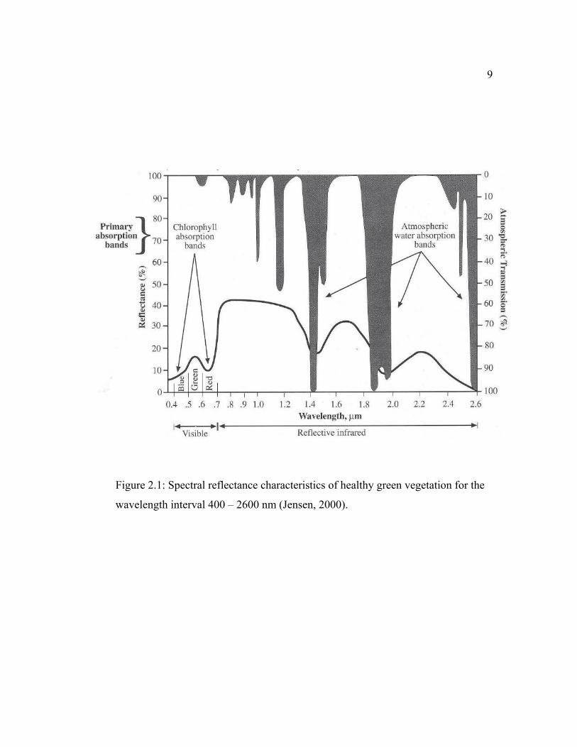
increases dramatically in the region from 700-1200 nm (see Figure 2.1). In the

near-infrared region, healthy green vegetation is generally characterized by high

reflectance (40 - 60 percent), high transmittance (40 - 60 percent) through the leaf

onto underlying leaves, and relatively low absorptance (40 - 60 percent) (Jensen,

2000). It was also pointed out that changes in the near-infrared spectral properties

of healthy green vegetation may provide information about plant senescence

9

Figure 2.1: Spectral reflectance characteristics of healthy green vegetation for the

wavelength interval 400 – 2600 nm (Jensen, 2000).

10 and/or stress. Near infrared region was emphasized for the vegetation study in that

the greatest percentage of incoming solar energy is accounted for in this

wavelength region, and canopy reflectance is typically an order of magnitude

greater in the near infrared region than in the visible region, thus changes in

reflectance are easier to measure and quantify (Williams, 1991).

Spectral properties of trees were studied either at the leaf (Daughtry et al., 1989)

or the canopy level (Gong et al., 1997; Aardt and Wynne, 2000) using a

spectrometer. Gong et al. (1997) reported experiments undertaken to classify six

conifers species (Douglas-fir, giant sequoia, incense cedar, ponderosa pine, sugar

pine and white fir) from hyperspectral measurements made at sunlit sides of tree

canopies in the field and tested the overall identification accuracy using artificial

neural network algorithm and linear discriminant analysis. Their experiments

indicated that the six conifer species could be identified with high accuracy while

the discriminating power of the visible region was stronger than the near-infrared

region. Aardt and Wynne (2000) tested the spectral differentiability among six

major forestry species (three pines; loblolly, Virginia and shortleaf pine and three

hardwoods; scarlet oak, white oak and yellow poplar) using canonical and normal

discriminant analysis. The cross-validation results within hardwood groups and

within pine groups indicated that they were separable, respectively as well as very

separable results between hardwood and pine groups.

Often, multi-scale studies integrating scale variations from leaf levels to canopy

or stand levels were carried out for the selected tree species using a spectrometer

for a small scale and for the larger scale study, either using remotely sensed data

such as Airborne Visible Infrared Imaging Spectrometer (AVIRIS) data (Asner,

1998; Roberts, 2004) or using helicopter-based remote sensing data (Williams,

1991). Jensen (2002) introduced fundamental concepts associated with vegetation

biophysical characteristics and how remotely sensed data can be processed to

provide unique information about these parameters. Since the 1960s, scientists

have extracted and modeled various vegetation biophysical variables using

remotely sensed data. Much of the effort has gone into the development of

11 vegetation indices – defined as dimensionless, radiometric measures that function

as indicators of relative abundance and activity of green vegetation, often

including leaf-area-index (LAI), percentage green cover, chlorophyll content,

green biomass, and absorbed photosynthetically active radiation (APAR) (Jensen,

2000). Among these, Normalized Difference Vegetation Index (NDVI), developed

by Rouse et al. (1974), was widely adopted and applied to the remotely sensed

data.

While the study of spectral reflectance using passively-sensed two-dimensional

images contributed to identification of tree species, due to the fact that they are

dependent upon reflected solar radiation which would cause the effects of

shadowing and bidirectional reflectance, they have limits in the capturing of three-

dimensional structure properties which might be one of the critical factors to

identify individual tree species.

2.2. LIDAR technology

LIDAR (Light Detection And Ranging) is one of the active optical remote sensing

technologies that can provide highly accurate measurements of both the forest

canopy and the ground surface. It provides data that make it possible to detect and

isolate individual trees and calculate attributes describing their size and form of

individual trees. Discrete-return, small-footprint LIDAR, one of the airborne

LIDAR systems, was used in this dissertation. Airborne laser scanning systems

have four major hardware components: (1) laser scanner, (2) differential global

positioning systems (GPS; aircraft and ground units), (3) a highly sensitive inertial

measurement unit (IMU) attached to the scanning unit, and (4) on-board computer

to control the system to store data from the first three components. The position

and attitude of the scanner at the time each pulse is emitted are determined from

data collected by the GPS and IMU units.

LIDAR systems used for topographic mapping applications usually operate in

the near infrared range of the spectrum (700-1200 nm). The most commonly used

12 lasers emit light at a wavelength of 1064 nm. Most systems have the capability of

acquiring multiple measurements (i.e., 2-5 per laser pulse). The scan angle is

typically limited to 15 - 20 degrees off-nadir allowing systems to acquire

measurements along a “swath” beneath the aircraft (see Figure 2.2). LIDAR

systems have a beam divergence of approximately 0.25- 4 mrad; therefore, the

“footprint” of the LIDAR pulse when it reaches the ground (or canopy surface) is

approximately 15 - 90 cm in diameter, depending upon flying height. For

topographic mapping applications, LIDAR data are acquired in leaf-off conditions

to maximize the percentage of pulses that reach the ground surface. For canopy

mapping or studying forest attributes, data are acquired in leaf-on conditions to

maximize laser returns from tree crowns and forest structures (McGaughey et al.,

2007).

2.2.1. LIDAR research for forestry applications

At the early stage of LIDAR research for forest applications, most of the emphasis

was on providing a characterization of ground topography, such as digital terrain

models using the unique ability of LIDAR to acquire direct vertical measurements

beneath the forest canopy among remotely sensed data. The vertical accuracy of

LIDAR terrain measurements was found to be in the range of 15-50 cm (RMSE)

depending on the conditions of topography (Kraus and Pfeifer, 1998; Pereira and

Janssen, 1999; Reutebuch et al., 2003).

Recently, research has focused on measurements of forest biophysical

characteristics mostly to estimate forest stand level parameters. The individual

tree-based approach was introduced by Samberg and Hyyppä (1999). Previously,

algorithms for delineation of individual tree crowns were developed uinsg high

resolution spectral images (Brandtberg, 1998; Gougeon, 1995; Pollock,

1996; Wulder et al., 2000). The accuracy of detecting individual trees has been

improved by combining laser scanning data with either digital aerial photography

13

Figure 2.2: Schematic showing the components of airborne laser scanning systems (LIDAR) (courtesy Robert J. McGaughey).

14 or spectral images. In most cases, individual tree-based research using laser data

focused on estimating forest parameters (Persson et al., 2002; Popescu et al., 2003).

Popescu et al. (2003) explored the feasibility of LIDAR data for estimating tree

crown diameters using variable window size techniques as well as other LIDAR-

measured parameters such as tree height and number of trees, to estimate forest

biomass and stand volume.

Tree species identification is important for a variety of natural resource

management and monitoring activities.,Some researchers became interested in the

study of classifying different tree species using LIDAR data (Brandtberg et al.,

2003; Brandtberg, 2007; Holmgren and Persson, 2004; McGaughey et al, 2005;

Moffiet et al., 2005; Song et al., 2002). In an earlier study, Song et al. (2002)

reported that conifers and broadleaf species can be distinguished by applying

filters to a grid of intensity data. Brandtberg et al. (2003) used leaf-off data to

describe the vertical structure of branches more clearly by assuming that the

absence of leaves in the canopy might facilitate the penetration of the laser beam

in a deciduous forest composed of oaks, red maple and yellow popular. They

indicated the potential for using leaf-off laser scanning data for species

classification of individual tree crowns. This study was later revised resulting in

better classification accuracy (Brandtberg, 2007). Holmgren and Persson (2004)

reported that Norway spruce and Scots pine could be identified with an overall

classification accuracy of 95% using two groups of variables such as features to

measure the shape of the trees and variables that do not measure the shape of the

tree such as intensity. McGaughey et al. (2005) used the same LIDAR data sets

used in this dissertation and reported that they could differentiate coniferous and

deciduous tree types using LIDAR intensity values from leaf-off data but not from

leaf-on data with a simple, intensity value threshold approach. Moffiet et al. (2005)

conducted exploratory data analysis to assess the potential of laser return type and

return intensity as variables for classifying white cypress pine(Callitrus

glaucophylla) and poplar box (Eucalyptus populnca). They found that

15 discrimination at the individual level was not always possible while the

discrimination was reliable at the stand level.

2.3. LIDAR data for this research

The study area for this research is located at the Washington Park Arboretum, an

urban green space on the shores of Lake Washington just east of downtown Seattle,

WA (see Figure 2.3). The area covers 230 acres and includes an impressive

collection of coniferous and deciduous trees and shrubs from around the world

including an assortment of tree species native to the Western United States.

This research utilized two LIDAR datasets collected over the Arboretum. The

first was acquired with an Optech ALTM 30/70 LIDAR system flown by

AeroMap in the summer of 2004 in leaf-on conditions. The second was acquired

with an Optech ALTM 3100 LIDAR system flown by Watershed Sciences, Inc.

(WS) in March of 2005 to obtain leaf-off conditions. The timing of the second

LIDAR flight was critical to ensure leaf-off conditions for the deciduous species.

Although originally intended, leaf-off conditions were not perfectly achieved with

the second dataset. Some trees had leaves, and/or flowers present. Digital photos

of individual trees were taken at the field site on the day of LIDAR acquisition and

aerial photographs were taken the day after the LIDAR acquisition to enable the

recognition of the leaf-off conditions. System specifications for both acquisitions

are shown in Table 2.1.

The laser scanning data were recorded in geographic (latitude, longitude)

coordinates. The LIDAR data have been re-projected to a UTM coordinate system.

The horizontal datum is NAD 83 UTM zone 10 meters, and the vertical datum is

orthometric heights based on a local CORS network. The data were provided in

ASCII text format, with the three-dimensional coordinates, intensity value, and

return number for each LIDAR return.

16 Aerial photographs Because some deciduous trees were starting to have foliage, aerial photographs

were taken from a fixed wing aircraft with a small-format digital camera, the day

after the leaf-off LIDAR acquisition, on March 18, 2005. These photographs

allowed me to detect deciduous trees that had obvious leaf growth or were in

bloom at the time of the LIDAR flight. An orthophotograph with a color image

acquired in leaf-on conditions in 2002, covering the arboretum was used in the

FUSION/LDV software (McGaughey and Carson, 2003; McGaughey et al., 2004)

to provide a frame-of reference for the LIDAR data.

2.3.1. LIDAR-based digital terrain model

Leaf-off LIDAR data were used to create a digital terrain model for the study area

because this laser system was flown with higher point density per square meter and

with more overlapped flight line than the system used for leaf-on conditions. The

Arboretum is relatively flat compared with conventional forest research sites. The

1 m x 1 m grid cell DTM was created using the FUSION/LDV software. The

method for creating DTM is well described in Andersen et al. (2006).

2.4. Field data collection for this research

2.4.1 Tree species selection for this research

To ensure analysis of various tree species with different biophysical characteristics

as well as representing deciduous and coniferous species groups, species were

selected based on macro characteristics such as crown shape and size and micro

characteristics such as leaf structure. Seven coniferous species were selected based

on leaf structure (Petrides and Petrides, 1992). The leaf-structure classifications of

the selected coniferous species are shown in Table 2.2. In addition to leaf

17

Some trees had leaves, and/or flowers present.

Figure 2.3: Approximate location of Washington Park Arboretum, Seattle, WA.

WASHINGTON

Washington Park Arboretum

18

Table 2.1: Laser scanner system specifications. Leaf-on data Leaf-off data

Acquisition date August 30, 04 March 17, 05

Laser wavelength 1,064 nm 1,064 nm

Laser scanner Optech ALTM 30/70 Optech ALTM 3100

Scan angle 22 o (11 o from Nadir) 20o (10o from Nadir)

Flying height above ground 1200 m 900 m

Scan pulse repetition frequency 71 kHz 100 kHz

Maximum number of returns

per pulse

3 4

Beam divergence 0.31 mrad 0.31 mrad

Scan width (approximate) 554 m 310 m

Flight line overlap 0 percent

(single flight line)

50 percent

Point density 2 to 5 points/m2 3 to 20 points/m2

19 structure, broadleaved species have various crown shapes and sizes which can be

easily distinguished even with aerial photographs (Lillesand and Kiefer, 1994).

The leaf-structure classifications of the eight selected broadleaf species are shown

in Table 2.3. For the selection of broadleaved species, crown shapes and sizes

were also considered as well as leaf structure. For example, bigleaf maple,

Quercus and elm have large crowns. The surface of Quercus crown is described as

billowy while elm has wide crowns with pitted tops. Sorbus has medium sized,

rounded crowns with undivided trunks (Lillesand and Kiefer, 1994). Betula has

various crown sizes depending upon species. Some of Prunus and Magnolia had

distinct white flowers over the crowns at the time of the leaf-off LIDAR data

acquisition. Both evergreen and deciduous species of Magnolia were sampled.

Plant names usually consist of two words, first the genus (such as Acer for

maples) and then the species epithet (such as macrophyllum for bigleaf maple).

That pair of words identifies uniquely a given plant species, which is a set of

natural populations of plants that can be distinguished clearly from all other

species (Omar, 1994). For the collection of non- Native species, “genus” might be

a correct terminology instead of “species” because there are a variety of species

within one genus. Therefore, the collected fifteen groups are composed of both

genera such as Prunus and species such as Douglas-fir (Pseudotsuga menziesii).

Because the goal of this research is to distinguish between genus not between a

variety of species within genus, to minimize complex usage of terminology,

“species” will be commonly used to represent each of the fifteen groups composed

of either “genus” or “species” in the later analyses.

2.4.2. Field measurements for this research

After the types of species were determined, individual trees were measured at the

Arboretum from April, 2005 through July, 2005. As part of the Arboretum’s

database, the locations of all living plants are recorded with their names and

conditions on the 100 x 100 feet grid cells over the Arboretum. The locations and

20 identification of non-native species were available from a trail map for visitors.

Plots for non-native species were chosen based on locations on the trail map while

plots of native species were chosen in areas where groups of individuals were

clustered. After plots were selected, a Trimble Pro XR/XRS GPS system was used

to record the geo-reference of the plot and the locations of individual trees. I

selected individual isolated trees to facilitate detecting and measuring individual

trees in the LIDAR point clouds. In total, twenty to twenty five individual trees

within each species were selected and measured. For each tree, stem diameter was

measured at 1.4 m above ground with a diameter tape and the species name was

recorded. Tree height, crown base height (CBH) and crown diameter (CD) were

also measured for each tree. Tree heights and CBH were measured using an

Impulse LR laser. CBH was measured as the distance along the stem from the

ground to the attachment of point of the first living branch. If the branch with live

foliage was widely separated from the above branch, the branch was not

considered within the crown (Holmgren and Persson, 2004). There are different

ways of measuring tree crown diameter depending on the purpose of research

(Schreuder et al., 1993). In this research, CD was measured to assist in detecting

individual tree locations in the LIDAR point clouds. Two perpendicular

measurements were obtained. One in the north-south direction through the center

of the stem was measured, and the other in the east-west direction crossing the

mid- point of the north-south length. Finally, field-measured CD was defined by

an average of the two perpendicular measurements. A summary of mean field

measurements for each species is shown in Table 2.4.

21

Table 2.2: Coniferous species used in this research.

Leaf structures Species

Clustered needles Evergreen Pinus

Deciduous Larch

Single needles On woody pegs Spruce

With flat needles Douglas-fir

Western hemlock

Redwood

Scale-like leaves Western red cedar

Table 2.3: Broadleaved species used in this research.

Leaf structures Species

Opposite simple leaves Bigleaf maple

Alternate compound leaves Sorbus

Alternate simple leaves Thorns Prunus

Malnus

Betula

Elm

Quercus

No thorns

Magnolia

22

Table 2.4: Summary of field measurements with the number of measured trees, mean stem diameters (DBH), mean heights, mean crown base heights (CBH) and mean crown diameters (CD) for each species.

Species

Number of trees

Mean DBH (cm)

Mean Height

(m)

Mean CBH (m)

Mean CD

(m)Broadleaved Betula 22 28.19 19.57 0.84 6.87

Bigleaf maple 20 64.12 21.67 5.47 13.17Elm 20 29.22 15.80 3.03 9.55Magnolia 25 37.10 20.71 1.34 12.21Malus 20 17.32 7.43 0.64 7.55Prunus 20 22.28 6.81 1.26 7.90Quercus 25 41.34 21.35 2.91 11.42Sorbus 20 13.10 7.51 1.57 4.75

Coniferous Western red cedar 23 84.72 24.95 1.21 10.07Douglas-fir 20 59.21 27.18 7.12 8.12Larch 25 62.35 24.81 2.23 12.27Pinus 25 51.69 23.04 3.66 7.94Redwood 20 71.27 21.76 0.34 8.63Spruce 22 33.82 16.97 0.15 6.58Western hemlock 20 13.86 33.53 2.59 10.85

23

Chapter 3

INDIVIDUAL TREE SPECIES IDENTIFICATION USING LIDAR

INTENSITY DATA

3.1. Introduction

While the greatest advantage of LIDAR over other remote sensing technologies is

its ability to capture 3-dimensional measurements over large areas, LIDAR

intensity data appears to contain valuable information relating to forest type and

condition. LIDAR intensity is a measure of the return signal strength. It measures

the peak amplitude of return pulses as they are reflected back from the target to the

detector of the LIDAR system. Intensity values vary depending on the flying

height, atmospheric conditions, directional reflectance properties, the reflectivity

of the target, and the laser settings.

For a diffuse target surface, completely illuminated by a given laser pulse, the

recorded intensity is related to the received power which can be given by the

following relationship (Baltsavias, 1999):

ttarr

r PR

DDMP 22

222

4 γρ=

where Pt and Pr are the transmitted and received power, Dr is the received aperture

size, Dtar is the target diameter, R is the range, γ is the beam divergence, M is the

atmospheric and bidirectional reflectance distribution function (πρ

) . The power

received by the sensor will be dependent on target characteristics, including the

physical properties of the target (diffuse vs. specular reflector) and absolute target

reflectivity. Range measurement is performed by multiplying the time interval (t)

between emission and reception of laser pulses by the speed of light (c):

24

2tcR =

With the aid of the flight path information (position and altitude of the LIDAR

system) each individual intensity measurement is time-synchronized with the

associated distance measurements. While LIDAR intensity data appears to contain

valuable information, its use is complicated by the fact that it is an uncalibrated

sensor. The fact that different LIDAR systems have different methods for

measuring intensity makes direct comparison of intensity data collected with

different scanners difficult.

While LIDAR intensity data have not been used as much as the three

dimensional structure data of laser returns, intensity data have been used in

conjunction with other variables in some studies. Brandtberg et al. (2003) used

indices derived from laser reflectance data as well as height of branches to classify

three deciduous species. Although they used a different terminology (laser

reflectance percentage instead of LIDAR intensity), they basically indicate the

same values. They concluded that most variables could be used for classification

purposes and discussed that different light and dark shapes of bark on the branches

were probably related to its capability to reflect the laser beam, which resulted in

differentiation of the deciduous species in leaf-off conditions. Holmgren and

Persson (2004) used two groups of variables, features that measure the shape of

the tree and other variables such as intensity for the purpose of identifying Norway

spruce and Scots pine. They discussed that the density of crowns and gaps within

the crowns affected different mean intensity values and standard deviations for the

two species. A new approach using a well-defined directed graph (digraph)

(Brandtberg, 2007) improved the classification accuracy markedly compared with

a previous study (Brandtberg et al., 2003) using both intensity data and more

reliable prediction based on shape characteristics of a marginal height distribution

of the whole first-return point cloud representing each tree.

Some researchers used intensity data as main basis for classification. Song et al.,

(2002) applied filters to a grided representation of intensity data and evaluated its

25 potential to classify different materials such as asphalt, grass, roof, and trees. They

concluded that LIDAR intensity can be used for land-cover classification and also

reported that the variance for trees is higher than other classes, possibly because

intensity varies with different species; the intensity of conifers was about 30%

while intensity of broadleaved trees was usually 60%. McGaughey et al. (2005)

used the same LIDAR datasets used in this research and found that they could

differentiate coniferous and deciduous tree types using the LIDAR intensity values

from the leaf-off data but not from the leaf-on data with a simple, intensity value

threshold approach. Moffiet et al. (2005) conducted exploratory data analysis to

assess the potential of laser return type and return intensity as variables for

classification of individual trees or forest stands according to species. They found

that discrimination at the individual tree level between white cypress pine

(Callitrus glaucophylla) and poplar box (Eucalyptus populnca) was not always

possible while the discrimination was reliable at the stand level. They also

indicated that return intensity statistics for the forest canopy, such as average and

standard deviation, were related not only to the reflective properties of the

vegetation, but also to the larger scale properties of the forest such as canopy

openness and the spacing and type of foliage components within individual tree

crowns. Hasegawa (2006) investigated the characteristics of LIDAR intensity data

for land cover classification and concluded that old asphalt and grass were

separable though zinc, brick, and trees were not easy to recognize. Soil, gravel,

and grass were distinguishable from one another in his research. Brennan and

Webster (2006) utilized lidar height and intensity data to classify various land

cover types using an object-oriented approach. They concluded that spectral and

spatial attributes of the lidar data were able to classify a variety of land cover types

using the derived surfaces, image object segmentation and rule-based classification

techniques. Recently, LIDAR intensity data was found to be directly related to

spectral reflectance of the target materials (Ahokas et al., 2006). They studied the

relationship between calibration of laser scanner intensity and known brightness

targets and concluded that intensity values were directly related to target

26 reflectance from all altitudes, 200 m, 1000 m, and 3000 m after correcting range,

incidence angle (both BRDF and range correction), atmospheric transmittance,

attenuation using dark object addition and transmitted power (difference in PRF

will lead to different transmitter power values).

Considering that tree species classification was studied by many researchers

using their distinct spectral reflectance, LIDAR intensity data has a potential for

the study of species classification especially when augmented with three

dimensional structure data. Because spectral reflectance changes depending upon

the time of a year for deciduous species (Gates, 1980), acquiring LIDAR datasets

in leaf-on and leaf-off conditions should be invaluable to study species

identification when dealing with various tree species. By analyzing intensity

values of various tree species with different characteristics such as a presence or

absence of foliage and spacing and type of foliage components within individual

tree crowns, the relative importance of the effect of different tree foliage on

intensity values can be evaluated.

The Washington Park Arboretum is a suitable field site to study forest

parameters at the individual tree levels due to the fact that individual trees can be

easily detected and measured and in many cases, tree crowns are not severely

overlapped. In terms of intensity analysis, extracting pure laser points belonging to

individual trees is important because previous researches have found that intensity

data is related to spectral reflectance which varies depending upon target materials.

Previously, researchers have developed methods of isolating individual trees

(Brandtberg et al., 2003; Persson et al., 2002; Popescu et al., 2002; Samberg and

Hyyppä, 1999). Their studies mainly focused on measuring forest parameters from

direct measurement such as tree height and crown diameter to stand level estimates

such as biomass and stand volumes, which are less sensitive to spectral signals of

laser returns originating from different materials. Because the intensity value

associated with each laser return varies depending on the target material, laser

returns belonging to neighborhood trees within individual tree crowns should be

excluded. This chapter describes an original method of isolating pure individual

27 trees and introduces variables related to LIDAR intensity values using isolated

individual trees. Mean intensity values of laser returns within individual tree

crowns were compared between species, crown portions, and return types in leaf-

on and leaf-off data, respectively. Pair-wise significance tests between tree species

were conducted using the Student’s two sample t-test. Due to the importance of

distinguishing broadleaf species and coniferous species for a variety of ecosystem

management activities, mean intensity values of these two species groups were

compared and classification accuracy was tested using linear and quadratic

discriminant analylsis.

3.2. Methods

3.2.1. Isolation of individual trees Because the variables used for analyses in this research describe individual tree

attributes, the following method for isolating individual trees within the LIDAR

point data was developed. First, individual trees were detected with the aid of

field-measured location data and isolated crudely in the laser point clouds. Next,

pure laser points belonging to each individual tree were extracted. All variables

were derived using laser returns that were located above the crown base height.

Crown base height was calculated using 0.5 m height layers (Holmgren and

Persson, 2004). To reduce the influence of laser points from low vegetation, a one-

dimensional median filter (size 9) was first applied on the array of height layers.

Each layer that contained less than 1% of the total number of non-ground laser

points within individual trees was set to zero and the others to one. The crown base

height was then set as the distance from the ground to the lowest laser data point

above the highest 0-layer found. The estimated crown base height was also used to

estimate crown length by deducting from the estimated tree height which was

calculated by the highest laser point within the isolated individual trees.

28 3.2.1.1. Crude isolation of individual trees As a first step to isolate returns from individual trees in laser point clouds, the

FUSION/LDV software (McGaughey and Carson, 2003; McGaughey et al., 2004)

was used to display the LIDAR point cloud near the approximate tree location. A

final location of each tree was assigned and the approximate crown diameter was

measured using the LIDAR data in FUSION/LDV with the aid of field-measured

tree height and crown diameters. McGaughey et al. (2004) discussed the

limitations of using this software when identifying and isolating individual trees in

areas where tree crowns overlapped. For the purpose to minimize such problems,

isolated trees were selected for measurement in the field however, some tree

crowns still overlapped. Laser returns less than 1 m above the ground surface were

omitted from the subsets to avoid the effects of laser points from the ground and

low vegetation. These laser points are called non-ground laser points. Next, the

laser points within the individual tree crowns were isolated within a cylinder

defined by field-measured location and crown diameters of each tree. Some field-

measured trees were excluded from further analysis if the tree could not be

identified in the laser point cloud or adjacent tree crowns overlapped the measured

tree. A final summary of the trees used for each species is shown in Table 3.1.

3.2.1.2. Extraction of pure laser points After LIDAR point clouds were isolated within the boundary of the approximate

crown diameters, pure laser points belonging to individual tree crowns were

extracted. If two tree crowns overlap, laser reflections from both trees are likely

mixed in the overlap area. Therefore, all laser points in the overlap area should be

excluded. Naturally, a crown surface tends to get lower from the top of the tree, or

from the crown center to the crown margin. Coniferous species usually have one

apex at or near the tree center, whereas broadleaved species often have a multiple

apices around the tree center. Therefore, the tree center was defined differently

depending on species: the treetop (highest point) was used for coniferous species

29 and the center of a tree crown using x and y coordinates of laser returns was used

for broadleaved species. The task of excluding laser points belonging to

neighborhood trees was conducted using the Interactive Data Language (IDL)

from Research Systems, Inc. The method of evaluating distributions of LIDAR

point clouds radially from the tree center to the crown margin consisted of three

stages:

(1) first, LIDAR point clouds within the boundary of crown diameters were

divided into eight, 45 degree sectors radially from the tree center to the

crown margin,

(2) for each sector, a new plot was created using the horizontal distance from

the tree center to the return and the return height, and

(3) mean heights for laser points were computed at every 0.5 m horizontal

distance interval starting from the tree center to the crown margin.

The length of the radial sample of laser points varies depending on the crown

radius, from the smallest one of 1.5 m (Sorbus) to the largest one of 11.5 m

(bigleaf maple). Using the trend of the computed mean heights for each 0.5 m

interval along the new x-axis, a transect, can be considered as three cases. For the

first case, mean point heights decrease from the tree center to the crown margin

consistently. In this case, the tree is assumed to be purely isolated and all laser

points were used for the later analysis. For the second case, mean point heights

start decreasing from the tree center but change into increasing in the middle of the

transect. In this case, there are two possibilities: one possibility is that some foliage

irregularly distributed within the crown, increasing the mean point heights in the

middle of the transect, and the other possibility is that two tree crowns overlap. For

cases when the foliage was irregularly distributed, the tree crown can be

considered as being isolated. For cases when tree crowns overlap, laser points

within the overlap area should be deleted. Therefore, criteria to separate these two

cases should be considered. If the trend of mean point heights increases in the

30 middle of the transect consecutively over a certain distance threshold, the tree

crown was assumed to overlap in that sector and the sector was excluded.

Otherwise, the tree was regarded as being isolated and all laser points were used

for later analysis. Three different scales were applied to the sectors for individual

trees depending on the crown size: 1) if average crown radius was less than 3

meters and the mean point heights increase more than two intervals (1 meter), the

sector was excluded, 2) if average crown radius was between 3 and 6 meters and

the mean point heights increase for more than three intervals (1.5 meters), the

sector was excluded, and 3) if average crown radius was over 6 meters and the

mean point heights increase more than four intervals (2 meters), the sector was

excluded. For the third case, mean point heights start increasing from the tree

center but change into increasing at the last a few intervals. In this case, two trees

are assumed to overlap around the edge of tree crowns and only the last intervals

where mean point heights increase were excluded. Again, three different scales

were applied to each sector of individual trees depending on the crown size: 1) if

average crown radius was less than 3 meters, the marginal intervals were deleted

up to two intervals (1 meter), 2) if average crown radius was between 3 and 6

meters, the marginal intervals were deleted up to three intervals (1.5 meters), and

3) if average crown radius was over 6 meters, the marginal intervals were deleted

up to four intervals (2 meters).

3.2.2. Computation of variables

Using the pure laser point clouds belonging to individual trees, variables were

computed to analyze intensity data and the proportion of first returns for tree

species. Mean intensity values for all laser returns were computed for the whole

crown, upper crown and crown surface within individual tree crowns in both leaf-

on and leaf-off data. The role of upper canopy to estimate forest stand level

parameters has been emphasized (Popescu et al., 2002). The laser points

positioned at the upper crown are less affected by overlapped areas than those at

31

Table 3.1: The number of individual trees for each species after isolating LIDAR point clouds within individual tree crowns.

Species

The number of Field-measured trees

The number of trees after isolation

Broadleaved Betula 22 20 Bigleaf maple 20 11 Elm 23 10 Magnolia 20 19 Malus 20 10 Prunus 25 11 Quercus 25 19 Sorbus 20 11

Coniferous Western red cedar 25 19 Douglas-fir 22 12 Larch 25 21 Pinus 20 21 Redwood 20 10 Spruce 20 15 Western hemlock 20 14

32 the whole crown and therefore they are likely to be laser points belonging to the

target tree. The uppermost 3m of the canopy observed in the field was open and

not overlapped in these data. Therefore, upper crown was defined as laser points

within 3 meters from the highest laser point. Some trees of Prunus, Malus and

Sorbus had crown lengths less than 3 meters. In these cases, laser points for the

whole crown were the same as those for the upper crown. Laser points

representing the crown surface were extracted after creating a canopy surface

model using FUSION/LDV software. All laser points were placed into 0.5 meter x

0.5 meter grid cell in x,y plane. Within each grid cell, the highest laser points were

selected and moved to the center of the grid cell. Connecting all center points with

corresponding elevation values within each cell, a canopy surface model was

created. This surface model drapes over the laser points. To analyze intensity

values for the crown surface, 1 meter and 0.5 meter buffers composed of laser

points directly below the corresponding elevation values were applied and

compared. One of the reasons to analyze intensity for the crown surface is that

laser points over the crown surface are likely to have more chances to hit leaves

than woody materials such as branches or stems in leaf-on conditions and therefore,

the intensity of the crown surface might better represent intensity of leaves.

Therefore, the two buffer sizes were used to obtain samples containing returns

representing foliage without eliminating too many laser points. Because there was

little difference between the 1-meter and 0.5-meter buffers when comparing mean

intensity values, the 1-m buffer was used for computing variables.

In most cases, first returns have the highest intensity values among other returns.

Intensity values for first returns are most easily interpreted since they represent a

direct, although uncalibrated, measurement of the reflectivity of the target material

(McGaughey et al., 2007). Mean first return intensity values were computed for

the whole crown, upper crown and crown surface. The proportion of first returns

was also calculated to help to explain the relationship between intensity values of

different return types.

33 To compare the variability of intensity among species, coefficient of variation of

intensity (CV) were calculated. CV, a standard deviation related to the mean, was

used instead of standard deviation because mean intensity values are assumed to

vary among species. Therefore, CV is expected to explain the variability between

trees composed of single materials and those of mixed materials such as leaves,

branches and stems.

Finally, the following nine variables representing intensity values as well as the

proportion of first returns were derived in leaf-on and leaf-off data for the

individual trees: (1) mean intensity values for the whole crown using all returns

(whole_all), (2) mean intensity values for the whole crown using first returns

(whole_1), (3) mean intensity values for the upper crown using all returns

(upper_all), (4) mean intensity values for the upper crown using first returns

(upper_1), (5) mean intensity values for the surface crown using all returns

(surface_all), (6) mean intensity values for the surface crown using first returns

(surface_1), (7) coefficient of variation of intensity values for the whole crown

using all returns (cv_all), (8) coefficient of variation of intensity values for the

whole crown using first returns (cv_1), and (9) the proportion of the first returns.

3.2.3. Statistical analysis

Species comparisons; Student’s t-test In addition to comparing mean intensity values for each tree species, Student’s t-

test was used to compare pairs of two species. The t-test is the most commonly

used method to evaluate the differences in means between two groups.

Theoretically, the t-test can be used even if the sample sizes are very small (e.g., as

small as 10; some researchers claim that even smaller n's are possible), as long as

the variables are normally distributed within each group and the variances of two

groups are equal.

34 Pearson's Correlation Pearson’s correlation was computed to find the relationship between variables

using all individual trees. The correlation between two variables reflects the degree

to which the variables are related. It is useful to compute correlations between

variables because if variables are closely related, all the variables don’t need to be

considered for the multivariate analyses and the additional variables sometimes

make further analyses more complicated. The most common measure of

correlation is the Pearson Product Moment Correlation (called Pearson’s

correlation for short). When computed from a sample, it is designated by the letter

“r” and is sometimes called “Pearson’s r”. Pearson’s correlation reflects the degree

of linear relationship between two variables. Pearson correlation coefficient is

written (Cohen, 1988):

where and are the sample means of X and Y , sx and sy are the sample

standard deviations of X and Y and the sum is from i = 1 to n. Pearson's r can

vary in magnitude from -1 to 1, with -1 indicating a perfect negative relationship, 1

indicating a perfect positive relationship, and 0 indicating no relationship between

two variables. In this research, Pearson’s correlation was computed using R

statistical package with all individual tree variables.

Discriminant analysis In forestry research, distinguishing individual broadleaved and coniferous species

is important. The validity of classifying these two groups can be tested using

discriminant analysis. Venables and Ripley (1994) described the functions first

explaining by sample covariance matrices:

W = gn

GMXGMX T

−−− )()( and B =

1)1()1(

−−−

gXGMXGM T

,

35 where W is the within-class covariance matrix, that is the covariance matrix of the

variables centered on the class means, and B is the between-classes covariance

matrix, that is of the predictions by the class means. M is g x p matrix of class

means, and G is the n x g matrix of class indicator variables (so gij = 1 if and only

if case i is assigned to class j). Consequently the predictions are the product of

matrices G and M. X is the vector of means of the variables over the whole sample.

Fisher (1936) introduced a linear discrimination analysis seeking a linear

combination, xa, of the variables which has a maximal ratio of the separation of

the class means to the within-class variance, that is maximizing the ratio aTBa /

aTWa.

In this research, discriminant analysis was conducted using discrim function in S

plus. All discriminant functions fit by discrim assume that the feature vectors are

normally distributed. A linear function is computed if the feature data covariances

are assumed to be equal among the groups, otherwise a quadratic function is

computed. Much of discrim and its methods are based on the lda and qda functions

and methods of the MASS library developed by Venables and Ripley (1994). In

this research, the two groups, broadleaf species and coniferous species, are tested

for the classification using lda and qda. The priori probability was set to 0.5,

which is suggested by Huberty and Olejnik (2006).

Principal components analysis Principal components analysis (PCA) is a technique used to reduce

multidimensional data sets to lower dimensions for analysis. Before doing

discriminant analysis, PCA was conducted to reduce correlated variables for

simplifying the later analysis. The basic idea of the method is to describe the

variation of a set of multivariate data in terms of a set of uncorrelated variables,

each of which is a particular linear combination of the original variables. The new

variables are derived in decreasing order of importance so that the first few

principal components (PCs) retain most of the variation present in all of the

36 original variables (Jolliffe, 2002). It is important to know how many PCs

adequately account for the given data set without serious information loss. Jolliffe

(2002) suggested several ways to decide on the number of components. In this

research, one way was chosen which compares unit variances of each principal

component (lk) and retain only those PCs whose variances lk exceed cut-off level.

Jolliffe (1972) suggested, based on simulation studies, that cut off l*= 0.7 is

roughly the correct level against the cut off l* = 1, originally suggested by Kaiser

(1960). After the number of components is determined, variables from the

unchosen set are added to the chosen set according to which has the greatest

absolute coefficient value on the component. In this research, principal component

analysis was conducted using R statistical package.

3.3. Results

3.3.1. Correlations between variables The results of Pearson’s correlation for the nine variables from 223 trees using two

matrices of scatterplots are shown in Figure 3.1 for leaf-on and in Figure 3.2 for

leaf-off data. The variable names are indicated on the diagonal. The data are

graphed on the lower left and their correlation coefficients (r) listed on the upper right.

Each square in the upper right corresponds to its mirror-image square in the lower left,

the "mirror" being the diagonal of the whole array. A set of mirror-image squares

indicates the correlation between two variables shown at the opposite directions of the

diagonal. The size of the font used for the numbers indicated in the upper right

squares was proportional to the resulting r values.

The six mean intensity variables were strongly positively correlated with each

other with r greater than 0.88 for leaf-on data (Figure 3.1). Leaf-off intensity

variables showed slightly stronger correlations, greater tan 0.95 (Figure 3.2).

Coefficient of variation of the first returns (cv_1) showed higher r values with

other variables than coefficient of variation for all returns (cv_all) in both leaf-on

37 and leaf-off data. CVs were negatively correlated with other mean intensity

variables and with the proportion of the first returns.

Figure 3.1: The scatterplot matrix of intensity-related variables and proportion of first returns in leaf-on data with Pearson’s correlation coefficients (whole_all —mean intensity for the whole crown using all returns; whole_1—mean intensity for the whole crown using first returns; upper_all—mean intensity for the whole crown using all returns; upper_1—mean intensity for the upper crown using first returns; surface_all-- mean intensity for the surface crown using all returns; surface_1—man intensity for the surface crown using first returns; cv_all—coefficient of variation using all returns; cv_1—coefficient of variation using first returns; prop_1—proportion of the first returns).

38

Figure 3.2: The scatterplot matrix of intensity-related variables and proportion of first returns in leaf-off data with Pearson’s correlation coefficients (whole_all — mean intensity for the whole crown using all returns; whole_1—mean intensity for the whole crown using first returns; upper_all—mean intensity for the whole crown using all returns; upper_1—mean intensity for the upper crown using first returns; surface_all-- mean intensity for the surface crown using all returns; surface_1—man intensity for the surface crown using first returns; cv_all—coefficient of variation using all returns; cv_1—coefficient of variation using first returns; prop_1—proportion of the first returns).

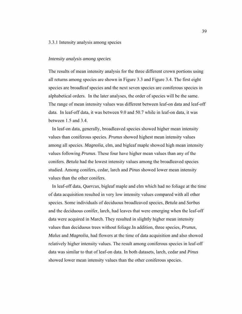
39 3.3.1 Intensity analysis among species

Intensity analysis among species The results of mean intensity analysis for the three different crown portions using

all returns among species are shown in Figure 3.3 and Figure 3.4. The first eight

species are broadleaf species and the next seven species are coniferous species in

alphabetical orders. In the later analyses, the order of species will be the same.

The range of mean intensity values was different between leaf-on data and leaf-off

data. In leaf-off data, it was between 9.0 and 50.7 while in leaf-on data, it was

between 1.5 and 3.4.

In leaf-on data, generally, broadleaved species showed higher mean intensity

values than coniferous species. Prunus showed highest mean intensity values

among all species. Magnolia, elm, and bigleaf maple showed high mean intensity

values following Prunus. These four have higher mean values than any of the

conifers. Betula had the lowest intensity values among the broadleaved species

studied. Among conifers, cedar, larch and Pinus showed lower mean intensity

values than the other conifers.

In leaf-off data, Quercus, bigleaf maple and elm which had no foliage at the time

of data acquisition resulted in very low intensity values compared with all other

species. Some individuals of deciduous broadleaved species, Betula and Sorbus

and the deciduous conifer, larch, had leaves that were emerging when the leaf-off

data were acquired in March. They resulted in slightly higher mean intensity

values than deciduous trees without foliage.In addition, three species, Prunus,

Malus and Magnolia, had flowers at the time of data acquisition and also showed

relatively higher intensity values. The result among coniferous species in leaf-off

data was similar to that of leaf-on data. In both datasets, larch, cedar and Pinus

showed lower mean intensity values than the other coniferous species.

40 Intensity analysis among different crown portions Generally, mean intensity values for the upper crown and crown surfacewere

higher than those for the whole crown in both leaf-on and leaf-off data. However,

mean intensity values for the crown surface for the three species, Malus, Prunus

and Sorbus were a little bit lower than those for the whole crown.

Significance tests for the mean intensity values between species To assess whether mean intensity values between tree species are significantly

different, a two-sample t-test was employed and compared. The results of

Student’s t-test for the mean intensity values for the whole crown are shown in

Table 3.2 and Table 3.3. The two tables display significant results by indicating

different significance levels with different colors based on p values: no-colored

cell indicates no significance (p>0.05), yellow-colored cell indicates medium

significance (** p<0.01, * p<0.05) and green-colored cell indicates high

significance (*** p<0.001). Eight broadleaved species were ordered alphabetically

from left to right sight (B1 to B8) and continuously seven coniferous species were

ordered alphabetically from left to right (C1 to C7). Table 3.4 shows the number of

significance t-tests within broadleaved, within coniferous and between

broadleaved and coniferous species in the leaf-on and leaf-off conditions.

Generally, pairs between broadleaved species and coniferous species showed

better separability than pairs within broadleaved species or within coniferous

species.. Most pairs in leaf-off conditions were significantly different. Except

several pairs within broadleaved species groups, each pair was very significant in

leaf-off data (p<0.001). In leaf-on data, even pairs between broadleaved species

and coniferous species were not always significantly different (p>0.05). Betula

(B1) which showed much lower mean intensity values than other broadleaved

species were significantly different from all other broadleaved species while they

were not significantly different from some coniferous species, cedar and larch

which showed lowest mean intensity values among conifers in leaf-on data. Except

41 pairs with Betula (B1), Quercus (B6) and a few pairs with Magnolia (B4), mean

intensity values of most pairs within broadleaved species were not significantly

different in leaf-on data. Quercus (B6) which showed second lowest mean

intensity values following Betula in leaf-on data showed high or medium

separability from other broadleaved species. Redwood (C6) which showed highest

mean intensity values among conifers showed poorer separability with

broadleaved species than with coniferous species in leaf-on data. Quercus (B6)

showed good separability from other broadleaved species, for example, p values of

all pairs were less than 0.01, while they didn’t show significant differences from a

few coniferous species such as Douglas-fir (C2), Pinus (C4), spruce (C6) and

western hemlock (C7) in leaf-on data. Larch (C3) showed good separability from

other species except from Betula (B1), Quercus (B6) and cedar (C1) in leaf-on

data.

Intensity analysis between return types The result of mean intensity values using all returns and using first returns for the

whole canopy are shown in Figure 3.5 and Figure 3.6. Predictably, for all species,

the mean intensity values using first returns were always higher than those using

all returns in both leaf-on and leaf-off datasets.

42

Figure 3.3: Mean intensity values for the three different crown portions in leaf-on data (whole_all—mean intensity values for the whole crown using all returns; upper_all—mean intensity values for the upper crown using all returns; surface_all—mean intensity values for the surface crown using all returns).

Figure 3.4: Mean intensity values for the three different crown portions in leaf-off data.

43 Table 3.2: The result of t-statistics between pairs of tree species for the mean intensity values for the whole crown using all returns in leaf-on data B1 B2 B3 B4 B5 B6 B7 B8 C1 C2 C3 C4 C5 C6 C7

B1

B2 ***

B3 ***

B4 ***

B5 ** ***

B6 ***

B7 *** ** ** *** * **

B8 *** *

C1 *** *** *** ** * *** **

C2 *** ** ** *** ** *

C3 *** ** *** *** *** ** ***

C4 ** *** ** *** * ** ** ** *

C5 *** ** *** * *** **

C6 *** ** ** *** ** * ** ** *

C7 *** ** ** *** * ** * ** **

*Note: no colored cell-no significance (p>0.05); yellow colored cell-medium significance (**p<0.01,*p<0.05); green colored cell-high significance (***p<0.001) Table 3.3: The result of t-statistics between pairs of tree species for the mean intensity values for the whole crown using all returns in leaf-off data

*Note: B1-Betula; B2-bigleaf maple; B3-elm; B4-Magnolia; B5-Malus; B6-Prunus; B7-Quercus; B8-Sorbus; C1-cedar; C2-Douglas-fir; C3-larch; C4-Pinus; C5-redwood; C6-spruce; C7-western hemlock

B1 B2 B3 B4 B5 B6 B7 B8 C1 C2 C3 C4 C5 C6 C7

B1

B2 **

B3

B4 *** *** ***

B5 *** *** *** ***

B6 *** *** *** ***

B7 *** *** *** ***

B8 ** ** *** ** ***

C1 *** *** *** *** *** *** *** ***

C2 *** *** *** *** *** *** *** *** ***

C3 ** *** *** *** *** *** *** *** *** ***

C4 *** *** *** *** *** *** *** *** ** *** ***

C5 *** *** *** *** *** *** *** *** *** *** *** ***

C6 *** *** *** *** *** *** *** *** *** *** *** ** ***

C7 *** *** *** *** *** *** *** *** *** *** *** *** *** **

44 Table 3.4: The number of significance t-tests within broadleaved, within coniferous and between broadleaved and coniferous species concerning mean intensity values for the whole crown in the leaf-on and leaf-off conditions.

# of non

significance

(leaf-on/-off)

# of

significance

at p<.05, .01

(leaf-on/-off)

# of

significance at

p< .001

(leaf-on/-off)

Total

(leaf-on/

-off)

Within broadleaved 14/7 6/4 8/17 28/28

Within coniferous 9/0 9/3 3/18 21/21

Between broadleaved

and coniferous

15/0

24/1

17/55

56/56

Intensity analysis between species with distinct flowers The conditions of individual trees in leaf-off data acquired on March 17th could be

roughly recognized via field survey conducted the same day and aerial

photographs taken the next day after LIDAR data acquisition. Two species, Prunus

and Magnolia, were easily recognized by their distinct white flowers covering the

crowns. However, some individuals within these species had not bloomed yet at

that time and therefore they had no-foliage. It is hypothesized that mean intensity

values for trees with and without flowers would be different. This hypothesis is

examined in this section.

Mean intensity values for trees with flowers and without flowers within these

two species are shown in Table 3.5 with the numbers of trees, standard deviation

of intensity values and p values as a result of two sample t-tests for the mean

intensity values. Mean intensity values were significantly different depending on

the presence or absence of flowers for both species that is, flowering trees showed

much higher mean intensity values than trees without flowers. Standard deviations

of intensity values were also significantly different with higher intensity values for

flowering trees than for non flowering trees.

45

Figure 3.5: Mean intensity values for the whole crown using first returns and all returns in leaf-on data (whole_all—mean intensity values for the whole crown using all returns; whole_1—mean intensity values for the whole crown using first returns).

Figure 3.6: Mean intensity values for the whole crown using first returns and all returns in leaf-off data.

46 Table 3.5: Mean intensity values for Magnolia and Prunus by separating trees with flowers from those without flowers in leaf-off data with the number of trees, the standard deviation of intensity values and the p-value from Student’s t-test.

Species Magnolia Prunus

Flowered No-flowered Flowered No-flowered

Number of trees 8 12 9 2

Mean intensity 48.15 11.29 38.36 11.99

Standard deviation 17.26 2.78 14.25 2.99

p-value <0.001 <0.001

Coefficient of variation of intensity values (CV) and the proportion of first returns The coefficient of variation of intensity values using first returns (cv_1) and all

returns (cv_all) and the proportion of first returns (prop_1) are variables which

don’t measure intensity of laser returns, directly. Instead, these variables are likely

to explain the relationship between returns. Therefore, CVs and the proportion

were compared among species. The results comparing these three variables among

tree species are shown in Figure 3.7 for leaf-on data and in Figure 3.8 for leaf-off

data.

Generally, there were no significant differences between cv_1 and cv_all for all

species in both datasets. Prominently, three short species, Prunus, Malus, and

Sorbus showed highest proportion of first returns in both datasets. Prunus and

Malus showed low variantions in both datasets. The three deciduous species,

bigleaf maple, elm and Quercus which had no foliage at the time of leaf-off data

acquired on March 17th, showed lowest proportion of first returns while they

showed highest CVs in leaf-off data. In leaf-on data, elm and bigleaf maple

showed relatively high proportion of first returns with higher values than conifers.

The results of coniferous species were more constant than those of broadleaved

species when comparing both datasets. Redwood showed lowest CVs among

conifers while Douglas-fir, larch and western hemlock showed high CVs in both

47 datasets. Douglas-fir showed relatively low proportion of first returns in leaf-on

data while they showed relatively high proportion in leaf-off data. The species

which showed high proportion of first returns seemed to show low CVs and vice

versa. Generally, there is a tendency that proportion of first returns was negatively

related to CVs among species.

Table 3.6 and Table 3.7 show the result of t-test for the CV using all returns in

leaf-on and leaf-off data. Table 3.12 shows the number of significance t-tests

within broadleaf species, within coniferous species and between coniferous and

broadleaved species. The result using leaf-off variables showed better separability

between species than using leaf-on variables. Betula (B1), bigleaf maple (B2) and

elm (B3) showed significant differences with all coniferous species (p<0.001).

Larch (C3) showed significant differences with all other coniferous species.

Prunus (B6) showed poor significant results with other species except with

Quercus (B7) where p value was less than 0.001. In the result using leaf-on

variables, pairs between coniferous species showed very poor significant results

except pairs between cedar (C1) and Douglas-fir (C2) where p value was less than

0.001. Betula were not significantly different from other species except with two

species, elm and Quercus where p value was less than 0.05.

Table 3.8 and Table 3.9 show the result of t-test for the CV using first returns in

leaf-on and leaf-off data. Table 3.13 shows the number of significance t-tests

within broadleaved species, within coniferous species and between coniferous and

broadleaved species. The leaf-off data showed better significant results than leaf-

on data, but not as good as the results for the CV using all returns.

Table 3.10 and Table 3.11 show the result of t-test for the proportion of first

returns in leaf-on and leaf-off data. Table 3.14 shows the number of significance t-

tests within broadleaved species, within coniferous species and between coniferous

and broadleaved species. It seems to be little difference between leaf-on and leaf-

off with leaf-off being somewhat weaker. In leaf-off data, Prunus (B6), Quercus

(B7), and Sorbus (B8) showed good separability from other species. In leaf-off

data, pairs between broadleaved species and coniferous species did not always

48 show better separability than pairs within broadleaved species. Generally, pairs

within coniferous species showed poor separability each other in both datasets.

Especially, redwood (C5) showed poor separability from other species in leaf-on

data.

3.3.2. Intensity analysis between broadleaved species and coniferous species

Mean intensity comparison among variables Mean values for the six intensity-related variables, coefficients of variation and

proportion of first returns for all broadleaved species combined and all conifers

combined were compared. Two-sample t-test was used to assess if these two

species groups were significantly different for each variable. The result is shown in

Table 3.15. With leaf-on data, the two species groups were significantly different

except for proportion of first returns which was not significant. For leaf-off data,

all variables were significantly different between the species groups. Broadleaved

species showed higher mean intensity values than coniferous species in leaf-on

data while they showed much lower values than coniferous species in leaf-off data

for all six intensity-related variables. Coefficient of variation of intensity (cv_1

and cv_all) showed lower values for broadleaved species than for coniferous

species in leaf-on conditions while they were higher for broadleaved species than

for coniferous species in leaf-off conditions. CV using all returns (cv_all) in leaf-

off data was less significantly different (p = 0.002) than most other variables.

Broadleaved species showed lower proportion (prop_1) than coniferous species in

leaf-off data (p = 0.002) but were not significantly different in leaf-on data.

To assess the separability of using each variable for the two species groups,

linear discriminant analysis was performed for each leaf-on, leaf-off, and

combined leaf-on and leaf-off datasets. The result is shown in Table 3.16.

Generally, variables based on leaf-off data showed better classification accuracy

than with leaf-on data. However, overall classification accuracy was improved by

49 combining leaf-on and leaf-off datasets. Among variables based on leaf-on data,

mean intensity for the whole crown with all returns (whole_all) showed best

accuracy (71.2 %) while among leaf-off variables, mean intensity for the upper

crown showed best accuracy (80.3 %). The result of combining variables based on

leaf-on and leaf-off datasets showed that classification accuracy was best for the

mean intensity for the whole crown using all returns (93.3%).

50 To simplify variables and compare classification accuracy between the leaf-on,

leaf-off and combined datasets, appropriate variables were derived using a

principal component analysis (PCA). With derived variables, linear discriminant

analysis (LDA) and quadratic discriminant analysis (QDA) were performed for

each dataset and the result is shown in Table 3.17. The accuracy was better in leaf-

off data than in leaf-on data in both LDA and QDA. Combining both datasets

improved the accuracy in both LDA and QDA.

In leaf-off data, broadleaved species contained species with flowers, Magnolia,

Malus, and Prunus at the time of data acquisition on March 17th. Also, larch is the

only deciduous species among coniferous species in the data of this dissertation.

Therefore, LDA and QDA were performed again for the sorted species groups

which are composed of deciduous broadleaved species and evergreen coniferous

species by excluding these four species. The result of classification accuracy with

these sorted species for each dataset is shown in Table 3.17. With leaf-off data, the

sorted species improved the classification accuracy up to 96.9 % for LDA and

94.8 % for QDA and for comibined datasets, they improved the accuracy up to

98.2 % for LDA and 95.5 % for QDA. However, the classification accuracy

decreased for leaf-on data using these sorted species. The improved accuracy

levels by combining both datasets compared with using leaf-off data were much

smaller than those by using leaf-off data compared with using leaf-on data, for

example, in case of using QDA for the sorted species, the improved accuracy was

0.7 % (95.5 % - 94.8 %) by using both datasets compared with using leaf-off data

while it was 35.0 % (94.8 % - 59.8 %) by using leaf-off data compared with using

leaf-on data.

51

Figure 3.7: The result for the proportion of first returns and coefficient of variation of the intensity using all returns and first returns for the whole crown concerning tree species in leaf-on data (prop_1—proportion of the first returns; cv_all—coefficient of variation of the intensity using all returns; cv_1—coefficient of variation of the intensity using all first returns).

Figure 3.8: The result for the proportion of first returns and coefficient of variation of the intensity using all returns and first returns for the whole crown in leaf-off data.

52 Table 3.6: The result of t-statistics between pairs of tree species for the coefficient of variation of intensity using all returns in leaf-on data. B1 B2 B3 B4 B5 B6 B7 B8 C1 C2 C3 C4 C5 C6 C7

B1

B2

B3 *

B4

B5 * *

B6 ** **

B7 ** *** ***

B8 *** **

C1 * ** ** ***

C2 ** *** *** *** * *** *** ***

C3 ** *** ** *** *** *** **

C4 ** ** *** *

C5 * ** ** *

C6 ** * ** *** ** *

C7 * * *

*Note: no colored cell-no significance (p>0.05); yellow colored cell-medium significance (**p<0.01,*p<0.05); green colored cell-high significance (***p<0.001) Table 3.7: The result of t-statistics between pairs of tree species for the coefficient of variation of intensity using all returns in leaf-off data. B1 B2 B3 B4 B5 B6 B7 B8 C1 C2 C3 C4 C5 C6 C7

B1

B2 *

B3 *

B4 * ** **

B5 *** *** ***

B6 *** ** ** ***

B7 ** ** ** ***

B8 * * *

C1 *** *** *** *** ***

C2 *** *** *** * ** *** *** ***

C3 *** *** *** *** *** *** ***

C4 *** *** *** * *** *** ***

C5 *** *** *** * ** *** * ***

C6 *** *** *** * *** ** *** *** *** **

C7 *** *** *** * *** *** *** *** *** **

B1-Betula; B2-bigleaf maple; B3-elm; B4-Magnolia; B5-Malus; B6- Prunus; B7- Quercus; B8- Sorbus;C1-cedar;C2-Douglas-fir;C3-larch;C4-Prnus;C5-redwood;C6-spruce;C7-western hemlock

53 Table 3.8: The result of t-statistics between pairs of tree species for the coefficient of variation of intensity using first returns in leaf-on data.

*Note: no colored cell-no significance (p>0.05); yellow colored cell-medium significance (**p<0.01,*p<0.05); green colored cell-high significance (***p<0.001) Table 3.9: The result of t-statistics between pairs of tree species for the coefficient of variation of intensity using first returns in leaf-off data.

B1 B2 B3 B4 B5 B6 B7 B8 C1 C2 C3 C4 C5 C6 C7

B1

B2 **

B3

B4 *

B5 *** *** *** **

B6 ** *** ** *

B7 *** *** ***

B8 *** **

C1 *** *** * * *** **

C2 ** *** *** * **

C3 ** *** *** ** ***

C4 *** *** *** ** *** *** ** *** ***

C5 *** *** *** *** *** *** ** *** ***

C6 *** *** *** * *** *** *** *** *

C7 ** *** ** ** *** ** *** *** *

B1-Betula; B2-bigleaf maple; B3-elm; B4-Magnolia; B5-Malus; B6- Prunus; B7- Quercus; B8- Sorbus;C1-cedar;C2-Douglas-fir;C3-larch;C4-Prnus;C5-redwood;C6-spruce;C7-western hemlock

B1 B2 B3 B4 B5 B6 B7 B8 C1 C2 C3 C4 C5 C6 C7

B1

B2

B3 **

B4

B5 *

B6 **

B7 * ** * **

B8 *

C1 * ** * ***

C2 *** *** ** ** ** *** ** **

C3 * *** *** *** *** *** *** ***

C4 * ** * *** *

C5 *

C6 ** *** * ** *** **

C7 ** *** * ** *** **

54 Table 3.10: The result of t-statistics between pairs of tree species for the proportion of the first returns in leaf-on data. B1 B2 B3 B4 B5 B6 B7 B8 C1 C2 C3 C4 C5 C6 C7

B1

B2

B3 *

B4 *

B5 *** *** ** **

B6 * ** *** ***

B7 *** *** * * ***

B8 *** *** ** ** ***

C1 *** *** *** * *** ***

C2 *** *** *** *** *** *** ***

C3 * ** *** *** *** ***

C4 * * *** ** *** *** *** *** **

C5 ** ** ** *

C6 * ** *** *** *** ** *

C7 *** *** *** *** *** *** ** * *

*Note: no colored cell-no significance (p>0.05); yellow colored cell-medium significance (**p<0.01,*p<0.05); green colored cell-high significance (***p<0.001) Table 3.11: The result of t-statistics between pairs of tree species for the proportion of first returns in leaf-off data.

B1 B2 B3 B4 B5 B6 B7 B8 C1 C2 C3 C4 C5 C6 C7

B1

B2 *

B3

B4 ** ***

B5 *** *** ***

B6 *** * *** ***

B7 *** *** *** *** ***

B8 *** *** *** *** ***

C1 * *** *** *** ***

C2 ** ** *** ** * **

C3 *** *** *** *** *

C4 * *** ** *** *** *** *** ***

C5 * *** ** * *** ** * ** **

C6 ** ** *** *** *** *** *** *

C7 *** *** *** *** * ** ** *

B1-Betula; B2-bigleaf maple; B3-elm; B4-Magnolia; B5-Malus; B6- Prunus; B7-Quercus;B8- Sorbus;C1-cedar; C2-Douglas-fir; C3-larch; C4-Pruns;C5-redwood;C6-spruce;C7-western hemlock

55

Table 3.12: The number of significant t-tests within broadleaved species, within coniferous and between broadleaved and coniferous species for the coefficient of variation of intensity using all returns in the leaf-on and leaf-off conditions.

# of non significance (leaf-on/off)

# of significance at p< .05, .01 (leaf-on/-off)

# of significance at

p< .001 (leaf-on/-off)

Total

(leaf-on/ -off)

Within broadleaved 18/9 7/13 3/6 28/28

Within coniferous 15/9 5/3 1/9 21/21

Between broadleaved and

coniferous

27/13

17/8

12/35

56/56

Table 3.13: The number of significant t-tests within broadleaved species, within coniferous and between broadleaved and coniferous species for the coefficient of variation of intensity using first returns in the leaf-on and leaf-off conditions.

# of non significance (leaf-on/-off)

# of significance at p< .05, .01 (leaf-on/-off)

# of significance at

p< .001 (leaf-on/-off)

Total

(leaf-on/ -off)

Within broadleaved 20/13 9/7 0/8 28/28

Within coniferous 18/6 3/6 0/9 21/21

Between broadleaved and

coniferous

21/19

18/12

17/25

56/56

Table 3.14: The number of significant t-tests within broadleaved species, within coniferous and between broadleaved and coniferous species for proportion of first returns in the leaf-on and leaf-off conditions.

# of non significance (leaf-on/-off)

# of significance at p< .05, .01 (leaf-on/-off)

# of significance at

p< .001 (leaf-on/-off)

Total

(leaf-on/ -off)

Within broadleaved 8/8 10/5 10/15 28/28

Within coniferous 11/10 9/9 2/2 21/21

Between broadleaved and

coniferous

18/18

10/14

28/24

56/56

56 Table 3.15: Mean intensity values for broadleaved and coniferous species for each variable with a p–value from Student’s t-test in leaf-on and leaf-off datasets. Variables Leaf-on data Leaf-off data

Broadleaved Conifer p Broadleaved Conifer p

whole_all 2.43 1.85 <0.001 18.91 33.11 <0.001

whole_1 2.52 1.97 <0.001 19.78 37.20 <0.001

upper_all 2.57 2.13 <0.001 20.56 41.35 <0.001

upper_1 2.54 2.12 <0.001 20.76 41.53 <0.001

surface_all 2.72 2.20 <0.001 19.65 36.42 <0.001

surface_1 2.74 2.20 <0.001 19.80 36.48 <0.001

cv_all 0.45 0.51 <0.001 0.60 0.53 0.002

cv_1 0.42 0.49 <0.001 0.56 0.43 <0.001

prop_1 0.82 0.79 0.12 0.73 0.81 0.002

Table 3.16: Classification accuracy for broadleaved and coniferous species for each variable using linear discriminant analysis with the leaf-on, leaf-off and combined datasets.

Classification accuracy (%) Variables Leaf-on Leaf-off All

whole_all 71.2 78.5 93.3

whole_1 69.9 79.4 91.0

upper_all 61.3 80.3 89.7

upper_1 60.9 80.3 90.1

surface_all 66.3 79.4 87.0

surface_1 68.1 79.8 87.0

cv_all 56.2 69.0 75.4

cv_1 69.9 71.7 82.0

prop_1 54.2 66.9 69.8

57 Table 3.17: Classification accuracies concerning two species groups with including all species and deleting four species using linear discriminant analysis (LDA) and quadratic discriminant analysis (QDA) for leaf-on, leaf-off and combined datasets.

All species Sorted species

Classification accuracy (%) Classification accuracy (%)

Variables

LDA QDA LDA QDA

Leaf-on 68.6 68.1 57.8 59.8

Leaf-off 82.5 83.9 96.9 94.8

All 88.8 90.6 98.2 95.5

3.4. Discussions

Correlations between variables The close correlation between mean values of the intensity variables implies that

these variables need to be reduced to simplify the further multivariate analyses.

Several authors have offered guidelines for the interpretation of a correlation

coefficient (r). Cohen (1988), for example, has suggested the rules of thumb: small

= 0.1 to 0.29, medium = 0.3 to 0.49 and large = 0.5 to 1.0 in psychological

research. As Cohen noted, however, all such criteria are in some ways arbitrary

and should not be observed too strictly. This is because the interpretation of a

correlation coefficient depends on the context and purposes. Therefore, instead of

evaluating absolute values indicated by r, comparing directions and relative

magnitudes between r values will be more appropriate.

Coefficient of variation (CV) was intended to be used for the purpose of

analyzing variability of intensity values among species instead of standard

deviations because standard deviations vary depending upon mean values.

However, the result of Pearson’s correlation implies that CV, a relative standard

deviation, also varies depending upon mean intensity values and therefore, it

58 doesn’t represent the variability of intensity values directly. Although the

proportion of first returns does not measure intensity values directly, it was

positively related to mean intensity values probably because intensity values of

first returns are usually higher than those of subsequent returns. This finding was

also reported by McGaughey et al. (2007).

Intensity analysis between broadleaved species and coniferous species Broadleaved species showed higher mean intensity values than coniferous species

in leaf-on data. Song et al. (2002) reported the same result using LIDAR intensity

data. Spectral reflectance of broadleaved species was found to be higher than that

of coniferous species by several studies in near-infrared wavelength regions.

Roberts et al. (2004) found that spectral reflectance of five broadleaved deciduous

species was higher than five conifers in near infrared wavelength regions at the

branch-scale. A recent finding that intensity data were directly related to spectral

reflectance of the target materials (Ahokas et al., 2006) implies that the result of

LIDAR intensity analysis in this research is consistent with the results of spectral

reflectance studies. Considering that spectral reflectance data are scale dependent,

a branch scale rather than leaf or landscape scale is probably applicable to LIDAR

study because the footprint of a LIDAR pulse is approximately 15-90 cm in

diameter depending upon flight height when it reaches the target materials.

Different intensity values between broadleaved species and coniferous species are

probably related not only to the reflective properties of the vegetation, but also to

the larger scale properties of the forest such as canopy openness and the spacing

and type of foliage components within individual tree crowns. For example, laser

pulses probably have a greater chance of passing through needles or scale-like

leaves than broad leaves. A pulse passing deeper into the crown would generate

multiple returns for each echo and consequently mean intensity values would be

lower within the crown and more likely associated with branches. If foliage is

distributed densely within the crown such as for Prunus, laser pulses would mostly

59 reflect from the crown surface which is mostly composed of leaves rather than

branches, which would result in higher percentage of first returns with higher

intensity values. In contrast, broadleaved species showed lower mean intensity

values than coniferous species in leaf-off data. This result is supported by Roberts

et al. (2004) who reported that bark has a lower spectral reflectance than leaves. In

leaf-off conditions, most laser pulses would reflect from woody materials such as

stems, branches and bark lowering reflectance of deciduous species relative to

non-deciduous species.

Intensity analysis among species In the leaf-on data analysis, Betula showed very low intensity values among

broadleaved species probably because Betula has a relatively sparse foliage

distribution increasing the chance that laser pulses reflect from branches. In

contrast, Prunus showed the highest mean intensity values probably because the

foliage distribution is very dense and so most of laser pulses would reflect from

leaves. Among coniferous species, Douglas-fir, western hemlock, redwood and

spruce showed higher intensity values than larch, cedar and Pinus in both leaf-on

and leaf-off datasets. This result seems to be related to their different leaf

structures. The former four species have single needles, whereas Pinus and larch

have clustered needles and cedar has small scale-like needles (Petrides and

Petrides, 1992). Species with single needles showed higher intensity than those

with clustered needles probably because clustered needles allow bare branches to

be exposed between them, which would raise the chance of laser pulses to reflect

from branches.

The result of separating individual trees with flowers from those without flowers

within Prunus and Magnolias in the leaf-off data acquired on March, 17th implies

that their flowers have distinctively higher mean intensity values than woody

materials such as stems and branches. Also the result of comparing standard

deviations of intensity for these separate groups implies that single materials such

60 as woody materials have much lower standard deviations than mixed materials

such as when flowers and branches or leaves and branches are both present. It

should be noted that standard deviations vary depending upon mean intensity

values and so the absolute values of standard deviations do not directly explain the

variability of intensity. Nevertheless, significantly different standard deviations for

different types of materials such as single versus mixed materials could explain the

variation in intensity within individual tree crowns. In this research, most of

Magnolia were deciduous but some were evergreen. Therefore, in leaf-off

conditions, Magnolia had either only white flowers or a mixture of white flowers

and leaves. Also the texture of leaves is different for evergreen Magnolia which is

leathery and deciduous Magnolia. However, no detailed analyses were conducted

on Magnolia in this research.

Overall, pairs of tree species showed very significant differences for the mean

intensity values for the whole crown in leaf-off data, even within broadleaved

species and within coniferous species. In leaf-on data, because overall mean

intensity values of broadleaf species were higher than those of conifers,

broadleaved species with low intensity values tend to show relatively poorer

separability from conifers. Similarly, conifers with high intensity values tend to

show relatively poorer separability from broadleaved species. Foliar conditions of

evergreen coniferous species are not very different between two datasets, although

in a dormant season, conifers shed older needles hence foliar density in March is

less than what would be present after the current year’s foliage has developed.

However, the pair-wise significance tests among coniferous species in leaf-on data

showed poor separability compared with leaf-off data. Two LIDAR datasets were

acquired from different laser scanner systems operated by different vendors. The

detailed descriptions of the two LIDAR datasets were presented in chapter 2.

Overall descriptions imply that the laser scanner system used to acquire leaf-off

data, Optech ALTM 3100, with a higher scan pulse repetition frequency, higher

point density per square meter and more overlap between flight lines could

describe each species better than that used to acquire leaf-on data, Optech ALTM

61 3070 in terms of intensity data. However, the relationship between each factor and

the resulting intensity data was not studied as part of this research.

Intensity analysis for different crown portions Mean intensity values for the upper portion and surface of the crown were higher

than those for the whole crown. This is probably because these portions of the

crown contain comparatively more leaves and younger leaves than the interior of

the crown with new buds blooming at the tip of branches. Rock et al. (1994)

supports this result by reporting that second year foliage showed lower reflectance

than first year foliage in near infrared wavelength regions. Mean intensity values

for the crown surface for three short species, Malus, Prunus, and Sorbus were

lower than those for the whole crown in leaf-off data. Considering the small size of

these species, a 1 meter buffer from the canopy surface model probably does not

represent the crown surface which is expected to contain more leaves and younger

leaves than the whole crown does. However, buffer thicknesses less than 1 meter

probably do not capture enough laser points. This result implies that analysis using

the upper portion of the crowns or crown surface crowns probably does not

provide useful information for these small-sized species.

Coefficient of variation of intensity and proportion of first returns Coefficient of variation of intensity (CV) and proportion of the first returns are not

direct measurements of intensity. However, the importance of these variables to

classify species types was discussed, previously. Moffiet et al. (2005) found that

proportion of singular returns was more useful than return intensity statistics such

as average and standard deviation to classify forest canopy for white cypress pine

(Callitrus glaucophylla) and poplar box (Eucalyptus populnca).

Three deciduous species, bigleaf maple, elm and Quercus, showed higher CVs

than other species in leaf-off data even though they contained only woody

materials without leaves. This is probably because their mean intensity values

62 were much lower (8.96, 11.92, and 10.92, respectively) than those of other species.

For example, mean intensity for evergreen conifers was 35.71 and the CVs were

relatively low. Therefore, it might not be easy to compare variability between

single and mixed materials using CV when mean intensity values are very

different. The proportion of first returns is probably related to crown length, too.

Short trees such as Malus, Prunus and Sorbus which have small crown lengths

probably have less chance to get subsequent returns, which results in a higher

proportion of first returns. Especially, Prunus have very dense foliage over the

crown so it is likely that laser pulses have little chance to pass through the crown

surface. This also caused lowest CV in leaf-on data analysis. Among broadleaved

species, Betula and Quercus which have relatively long crowns and sparse foliage

showed higher CVs. The ranks among coniferous species based on the results were

constant for leaf-on and leaf-off data. However, it is hard to explain which factors

influence the results.

Predictably, significance tests between pairs of species using the CVs showed

that more pairs had significant differences in leaf-off data than in leaf-on data.

This is probably because the variability of mean intensity values between species

is much higher in leaf-off data than in leaf-on data.

McGaughey et al. (2007) reported that first returns have the highest intensity

values and intensity values for subsequent returns are lower than the intensity of

the first return. This research is consistent with those results; mean intensity values

using only first returns were always higher than those that included all returns for

all species in both leaf-on and leaf-off data.However, the difference was small.

This is probably because not only multiple returns but also singular returns exist

within the crown. That is, if a singular return reflects from woody material, the

intensity is probably lower than second or third returns which would reflect from

leaves even though the singular return is the first return. This probably affects the

small difference between mean intensity using first returns and all returns. The

result of Pearson’s correlations between mean intensity variables for the upper

portion and surface of the crown showed that correlation coefficients between

63 mean intensity of all returns and first returns were high in both leaf-on and leaf-off

datasets. It is probably because these portions of the crown are mainly composed

of first returns, which results in small differences between two variables, mean

intensity values using all returns and first returns.

Discriminant analysis The result of discriminant analysis implies that combining leaf-on and leaf-off

datasets would be better to classify broadleaved species and coniferous species

than using data from one season. However, trade-offs should be considered

between the cost of acquiring additional LIDAR data and the improvement in the

classification accuracy. In fact, analysis that combined variables from leaf-on and

leaf-off data (see Table 3.17) showed that combining leaf-on with leaf-off

variables didn’t improve classification accuracy very much. Therefore, for the

purpose of classifying these two species groups, using LIDAR data in leaf-off

conditions is recommended because leaf-off variables resulted in better

classification accuracy. The problem is that it is not always easy to predict the

exact timing of leaf-off conditions for various deciduous tree species. It varies

depending on not only species but also the weather and locations. Scheduling

flights for very specific dates can be very hard.

Because leaf-off LIDAR data were acquired in mid March, it was not perfectly

leaf-off conditions for some species. Also, larch is the only deciduous coniferous

species in these data and so it is probably distinctive from the other six evergreen

coniferous species in the leaf-off data. Predictably, classification accuracy was

improved using the leaf-off dataset by deleting three broadleaved species,

Magnolia, Malus and Prunus and one coniferous species, larch. This result implies

that if LIDAR datasets can be acquired during the winter with complete leaf-off

conditions, broadleaved species can be well distinguished from coniferous species.

Predictably, the classification accuracy decreased using the same methodology

with the leaf-on data. This is probably because these species are not different from

64 the others in late summer and only reduced the overall sample size from 223 to

162. The presence or absence of foliage in deciduous species changes seasonally

and blooming timing varies depending upon species. Because results revealed that

the intensity values were different for trees with and without flowers (see Table

3.5), it would be helpful to know when each species blooms prior to selecting the

date for data acquisition.

3.5. Conclusions

The overall results showed that LIDAR intensity values could distinguish

various tree species and distinguish broadleaved species from conifers. Different

intensity values between species were related to not only reflective properties of

the vegetation, but also a presence or absence of foliage and the arrangement of

foliage and branches within individual tree crowns. Two different seasonal LIDAR

datasets resulted in different intensity values for the same species with better

separation results using the LIDAR data acquired in March than using that in

August.

65

Chapter 4

INDIVIDUAL TREE SPECIES IDENTIFICATION USING

LIDAR-DERIVED STRUCTURE MEASUREMENTS

4.1. Introduction

The previous chapter focused on analyzing LIDAR intensity data to differentiate

species. Historically, LIDAR technology has been used to capture and detect the 3-

dimensional structure of objects. Nelson (1997) reported the effect of different

canopy shapes on simulated laser measurements of height and estimates of basal

area, volume and biomass derived via simulation. Although his study focused on

modeling forest canopy heights, he assumed a particular tree’s canopy, in profile,

was one of four geometric shapes: cone, paraboloid, ellipsoid, or spheroid. He

recommended that tree canopy shapes should be noted when field data were

collected for purposes of height simulation but, he didn’t try to derive tree canopy

shapes directly from laser points. Popescu and Wynne (2004) assumed that

deciduous trees and pines had different relationships between tree height and

crown width for estimating plot-level tree height by measuring individual trees

identifiable on the three-dimensional lidar surface. They tried to find the best

fitting model for each group and found that the two groups had different models.

They found that filtering for local maximum with a circular window produced

better results for pines and filtering with a square window provided slightly better

results for deciduous trees. Their study implies that simple measurements such as

crown length to width ratio can be used to separate deciduous trees and pines.

Several authors report efforts to distinguish tree species using positions of laser

points within individual tree crowns as well as intensity data. Brandtberg et al.

(2003) used indices derived separately for the height and laser reflectance of

66 branches to classify three deciduous species, oaks, maples and yellow poplars.

They suggested that most variables could be used for classification purposes and

implied that when several single variables were combined, the classification

accuracy was improved. They used different height-related variables for the

returns, but they didn’t test the capability to distinguish crown shapes between the

species. Later, Brantberg (2007) replaced the previously unreliable height

estimates based on the maximum single laser point for each tree with a more

reliable prediction based on shape characteristics of the marginal height

distribution of the whole first-return point cloud for each tree. He reported that the

new method improved classification accuracy markedly. Holmgren and Persson

(2004) tried to detect crown shapes more directly using LIDAR data. They used

features that measure the shape of the tree such as relative crown base height,

relative height percentiles and parameters from the parabolic surface to identify

Norway spruce and Scots pine. They reported that spruce trees were usually more

conical and therefore have a lower 90th height percentile compared with pine trees.

They also noted that the parameters from the parabolic surface generally had a

higher negative value for spruce trees compared with pine trees. However, they

discussed that the shape of the crown could also be influenced by competition

from neighboring trees, making the shape of a pine tree more conical, similar to a

spruce tree and therefore, using only the shape gave low classification accuracy.

They found that higher classification accuracy was achieved when using both

variables related to intensity data and shape features. The studies didn’t test the

ability to differentiate between broadleaved species and coniferous species.

Brandtberg et al. (2003) used only three broadleaved species while Holmgren and

Persson (2004) used only two coniferous species. Therefore, the use of shape

variables to differentiate coniferous species from broadleaved species has not been

investigated.

In this chapter, variables derived from LIDAR to describe crown shapes are

presented mainly for the purpose of distinguishing broadleaved species from

coniferous species at the individual tree level. Also, variables using height

67 percentiles of laser returns were calculated. The isolation method described in the

section 3.2.1 is rather conservative and focused on measuring intensity values.

However, the method is still applicable when analyzing crown shapes if we use

upper portions of a crown where there is less overlap and the crown shape is less

affected by competition with other trees. Length to width ratio within upper

portions of a crown was derived and significance test was conducted for

broadleaved and coniferous species using Student’s two-sample t-test.The

classification accuracy was tested through discriminant analysis.

4.2. Methods

4.2.1. Crown structure measurements

The vertical distribution of laser points has been used in many forestry

applications. The goal of such research was to estimate plot-level tree height,

which was subsequently used to estimate basal area, biomass and volume. Vertical

distributions of laser points within individual tree crowns might not fully describe

crown shapes for a tree species. However, these variables are likely to be useful to

classify tree species with the accurate vertical measurements using LIDAR

technology. Relatively little lidar research dealing with crown diameters at the

individual tree level has been reported. Popescu et al. (2002; 2004) derived a

prediction for crown width using linear regression based on the field measured

height and crown diameters for pines and deciduous trees although he noted that

the relationship was not as strong as between DBH and height using only height as

the predictor variable.

4.2.1.1. Vertical distributions of laser returns

Different height percentiles were tested to differentiate tree species (Holmgren and

Perssons, 2004). They found that relative 90th height percentiles which was

68 defined as the 90th height percentile of laser returns divided by the maximum laser

return height within individual tree crowns were related to canopy shapes. For

example, more conical shapes have lower values for the relative 90th height

percentiles. In this research, different height percentiles were used and also

standard deviations of laser return heights were used. The standard deviation is an

additional characteristic of the vertical structure. Based on the height (distance

from the ground) of laser returns within the isolated individual trees derived in the

section 3.2.1, relative values were obtained by dividing by the estimated tree

height. Using IDL, relative 10th height percentile, relative 90th height percentile,

relative median height percentile, and relative standard deviation of height were

computed for each tree in both leaf-on and leaf-off datasets.

4.2.1.2. Upper crown shape

When trees overlapped at the edge of the crown, the laser returns positioned at the

edge were ignored according to the section 3.2.1. Therefore, structure-related

variables for the whole crown would be less reliable than those for the upper

crown. Trees with conical shapes are likely to have longer crown length compared

with crown width than trees with round shapes at the upper portion of the crown.

For each individual tree, average width was computed by averaging the maximum

distance which was computed as Euclidean distance using x and y coordinates of

laser returns from the tree center to the farthest laser returns at each 45 degree

radial sector. Three different portions of an upper crown were used: upper 10%,

upper quarter (25 %) and upper a third (33.3%) of the crown length. At each

portion of an upper crown, length to width ratio was computed.

4.2.2. Statistical analysis

Using Pearson’s correlation described in the section 3.2.3, correlations between

structure-related variables were computed using the R statistical package. One

69 variable, proportion of the first returns, which was derived in chapter 3 was used

again to find the relationships with other structure-related variables in this chapter.

Student’s t-test was used to evaluate significant differences between broadleaved

species and coniferous species for each variable. Linear discriminant analysis was

also used to test the classification accuracy for the two species groups. The eight

structure-related variables derived from leaf-on and leaf-off datasets were

compared separately and in combination to assess the classification accuracy using

linear and quadratic discriminant analysis (LDA and QDA), after reducing the

number of variables using principal component analysis (PCA). The details of

LDA, QDA and PCA methodology are described in the section 3.2.3.

4.3. Results

4.3.1. Correlations between structure variables

The results of Pearson’s correlations for the eight variables from 223 trees using

scatterplot matrices are shown in Figure 4.1 for leaf-on data and in Figure 4.2 for

leaf-off data. The variable names are indicated on the diagonal. The data were

graphed in the lower left and their correlation coefficients (r) listed in the upper

right. Each square in the upper right corresponds to its mirror-image square in the

lower left, the "mirror" being the diagonal of the whole array. A set of mirror-

image squares indicates the correlation between two variables shown at the

opposite directions of the diagonal. The size of the font used for the numbers

indicated in the upper right squares is proportional to the size of the resulting r

values.

Correlation coefficients (r) between height-related variables such as relative 10th

height percentile (rel10th), relative 90th height percentile (rel90th) and relative

median height percentile (relmed) showed high positive values while r between

crown shape-related variables, length to width ratio within an upper 10% (ratio10),

25% (ratio25) and 33% (ratio33) of a crown length, showed relatively low values

70 with the both leaf-on and leaf-off data. Relative standard deviations of heights

(relstdev) showed negative relations with three height percentiles. Four height-

related variables, rel90th, relmed, rel10th and relstdev, in leaf-off data showed

stronger correlations than those in leaf-on data. The proportion of first returns

(prop_1) showed relatively low correlations with most of other structure-related

variables. Expectedly, the same counter parts between variables for the two

datasets showed similar trends in terms of the direction and the degree of

correlations. For example, if two variables, relative 10th height percentile and

relative standard deviation of heights, were strongly negatively correlated in leaf-

on data, they also showed a similar relationship in leaf-off data.

71

Figure 4.1: The scatterplot matrix of structure variables in leaf-on data with Pearson’s correlation coefficients (rel10th, relmed and rel90th—relative 10th , 50th, and 90th height percentile; relstdev—relative standard deviations of heights; ratio10, ratio 25 and ratio 33—length to width ratio within an upper 10%, 25% and 33% of a crown length; prop_1—proportion of first returns).

72

Figure 4.2: The scatterplot matrix of structure variables in leaf-off data with Pearson’s correlation coefficients (rel10th, relmed and rel90th—relative 10th , 50th, and 90th height percentile; relstdev—relative standard deviations of heights; ratio10, ratio 25 and ratio 33—length to width ratio within an upper 10%, 25% and 33% of a crown length; prop_1—proportion of first returns).

73 4.3.2. Vertical distributions of laser returns

The results of three relative height percentiles and the relative standard deviations

of heights for each species in leaf-on and leaf-off data are shown in Figure 4.3 and

Figure 4.4, respectively. Species are ordered in eight broadleaved species followed

by seven coniferous species in an alphabetic order.

Generally, the higher the 10th height percentiles (rel10th), the lower the standard

deviations of heights (relstdev) in both datasets. There were few differences

between mean values of the 90th height percentiles among species. The results for

coniferous species were consistent between the two datasets while the results for

broadleaved species were somewhat different between them. Pinus showed the

highest values for the three relative height percentiles among coniferous species

while Douglas-fir and larch showed the lowest 10th height percentiles (rel10th) and

relative median heights (relmed) in both datasets. Elm showed high values for the

height percentiles in leaf-on data while they showed comparatively lower median

heights (relmed) and 10th height percentiles (rel10th) in leaf-off data. The height

percentiles for bigleaf maple were lowest among broadleaved species in leaf-off

data while they were relatively high in leaf-on data. Prunus showed the highest

10th percentiles (rel10th) in leaf-off data and had the lowest standard deviation of

heights (relstdev) in both datasets.

Significance tests between broadleaved species and coniferous species The results of the two-sample t-tests for broadleaved species and coniferous

species for each variable are shown in Table 4.1 for leaf-on data and in Table 4.2

for leaf-off data. The p-value was indicated with group means for each variable. In

leaf-off data, the two species groups didn’t show significant differences for any

variables (p<0.05) while in leaf-on data, they showed significant differences for

the three height percentiles (p<0.01) with higher mean values for broadleaved

species.

74

Figure 4.3: Mean values for four height-related variables for each species in leaf-on data (rel10th, relmed and rel90th—relative 10th, 50th, and 90th height percentile; relstdev—relative standard deviations of heights).

Figure 4.4: Mean values for four height-related variables for each species in leaf-off data.

75 Table 4.1: The p- value for Student’s t-test and mean values for four height-related variables for broadleaved species and coniferous species with the leaf-on data.

Group means

Variable Broadleaved Coniferous

p

Relative 10th height percentile 0.458 0.403 0.006

Relative median height percentile 0.720 0.670 0.001

Relative 90th height percentile 0.929 0.907 0.001

Relative standard deviations 0.182 0.187 0.483

Table 4.2: The p- value for Student’s t-test and mean values for four height-related variables for broadleaved species and coniferous species with the leaf-off data.

Group means

Variable Broadleaved Coniferous

p

Relative 10th height percentile 0.470 0.444 0.337

Relative median height percentile 0.698 0.682 0.159

Relative 90th height percentile 0.901 0.891 0.285

Relative standard deviations 0.163 0.169 0.373

4.3.3. Length to width ratio within upper portions of a crown

The result for length to width ratio within different portions of an upper crown is

shown in Figure 4.5 for leaf-on data and in Figure 4.6 for leaf-off data. Coniferous

species showed much higher ratio than broadleaved species in both datasets.

Generally, the ratios were higher in leaf-off data than in leaf-on data, especially for

broadleaved species. Betula and Magnolia showed a great increase from leaf-on to

leaf-off and became as high as some coniferous species. Among coniferous species,

Pinus showed very low ratio in both datasets. In leaf-on data, the ratio within an

upper 10% of a crown length was higher than those within an upper 33% of a

76 crown length for all species. However, in leaf-off data, the ratio varied depending

on species, that is, some species had higher ratio within an upper 33% of a crown

length than those within an upper 10% of a crown length.

The result of Student’s t-test for broadleaved species and coniferous species for

each variable is shown in Table 4.3 and Table 4.4 with mean and p-values. In

addition, classification accuracy using linear discriminant analysis was tested and

compared between variables. The result is shown at the last column for each

variable in Table 4.3 and Table 4.4. In both datasets, broadleaved species and

coniferous species showed significant differences using t-statistics (p <0.001) with

higher mean values for coniferous species. Overall, the accuracies were higher in

leaf-on data except for the ratio within an upper 10% of a crown length where leaf-

off data showed higher accuracy (58.2%) than leaf-on data (55.3%). In leaf-on data,

the ratio within an upper 33% of a crown length showed the highest classification

accuracy (61.3%) and the ratio within an upper 10% of a crown length showed the

lowest accuracy (55.3%) while in leaf-off data, the ratio within an upper 10% of a

crown length showed the highest classification accuracy (58.2%) and the ratio

within an upper 33% of a crown length showed the lowest accuracy (46.5%).

77

Figure 4.5: The result for length to width ratio at the upper 10 %, 25 % and 33 % of a crown length in leaf-on data (upper 10%, 25% and 33%—length to width ratio within an upper 10%, 25% and 33% of a crown length).

Figure 4.6: The result for length to width ratio within an upper 10 %, 25 % and 33 % of a crown length in leaf-off data.

78 Table 4.3: The p- value for Student’s t-test and mean values for length to width ratio within three different portions of an upper crown and the classification accuracy using linear discriminant analysis with the leaf-on data.

Group means Variables

Broadleaved Coniferous

p Classification

accuracy (%)

Ratio at upper 10 % 1.13 2.01 <0.001 55.3

Ratio at upper 25 % 1.02 1.92 <0.001 58.7

Ratio at upper 33 % 0.60 1.41 <0.001 61.3

Table 4.4: The p- value for Student’s t-test and mean values for length to width ratio within three different portions of an upper crown and the classification accuracy using linear discriminant analysis with leaf-off data.

Group means Variables

Broadleaved Coniferous

p Classification

accuracy (%)

Ratio at upper 10 % 1.35 2.18 <0.001 58.2

Ratio at upper 25 % 1.15 2.02 <0.001 54.4

Ratio at upper 33 % 0.76 1.70 <0.001 46.5

4.3.4. Discriminant analysis using all structure variables

The result of classification accuracy for broadleaved and coniferous species using

structure variables selected by principal component analysis for the variables

based on leaf-on, leaf-off and the combined datasets using linear discriminant

analysis (LDA) and quadratic discriminant analysis (QDA) are shown in Table 4.5.

The result of LDA and QDA were different depending on the variables used. The

overall result shows that the classification accuracy was better using leaf-on data

than using leaf-off data in both LDA and QDA. The classification accuracy for the

variables based on leaf-off data using LDA was much lower than the other cases.

When leaf-on and leaf-off data were combined, accuracy improved for QDA but

decreased slightly for LDA.

79 Table 4.5: Classification accuracies concerning the two species groups for the structure variables selected by principal component analysis for leaf-on, leaf-data, and combined datasets using linear discriminant analysis (LDA) and quadratic discriminant analysis (QDA).

Variables LDA (%) QDA (%)

Leaf-on 74.9 75.8

Leaf-off 50.2 72.2

All 74.0 78.5

4.4. Discussions

Correlations between variables Relative 10th height percentiles (rel10th) seem to be related to relative crown base

height, that is, trees with higher relative crown base height tend to have higher

relative 10th height percentile. If the relative crown base height is lower, then the

relative crown length is longer, which probably results in higher relative standard

deviations (relstdev). This is consistent with the result that rel10th and relstdev

were strongly negatively correlated in both datasets. The low correlations between

the variables based on length to width ratio within different portions of an upper

crown are probably because either the ratios within upper crowns vary depending

on the heights, or the method of computing the variables does not capture the

crown shapes. In fact, because we calculated each measurement based on the

distance between laser returns, the density of laser returns within the individual

tree crowns affects the accuracy of the data analysis, although both datasets,

especially leaf-off data, had high return densities. The proportion of first returns

does not have close correlations with either intensity variables or structure

variables based on the result in this chapter and chapter 3.

80 Vertical distributions of laser returns Although Holmgren and Persson (2004) reported that relative 90th height

percentiles (rel90th) was related to crown shapes, the difference between the

variables, rel90th, among species was small in this research. However, among

coniferous species, the rel90th was highest for Pinus which has relatively a round

crown shape among coniferous species in both leaf-on and leaf-off datasets.. A

few deciduous species showed different results between leaf-on and leaf-off

datasets probably due to the presence or absence of foliage. For example, bigleaf

maple and elm showed comparatively lower height percentiles in leaf-off than in

leaf-on data. This is probably because leaf-off conditions allow more laser returns

to pass through the canopy, lowering the position of laser returns. However,

relative height percentiles also might vary depending on the laser point density

from different laser scanning systems and so it is hard to compare the results from

the two different datasets directly.

Vertical distributions of laser returns didn’t distinguish broadleaved species and

coniferous species well. Leaf-on data showed better results than leaf-off data for

separating two species groups, probably because broadleaved species have higher

relative height percentiles than coniferous species in leaf-on conditions, however,

in leaf-off conditions in March for some deciduous species might have allowed

more laser returns to pass through the canopy, lowering the overall position of

laser returns. Therefore, the difference between two species groups for these

variables would be smaller in leaf-off data.

Length to width ratio within upper portions of a crown Expectedly, broadleaved and coniferous species showed significant differences for

length to width ratio within all three portions of an upper crown using t-statistics

(p<0.001) in both leaf-on and leaf-off datasets. Conical crown shapes are expected

to have higher ratios than round shapes for the upper crowns and this was

consistent with the result of this research. In this chapter, although simple ratios

81 were computed using length and average width within portions of the upper crown,

they can be regarded as describing the crown shapes between broadleaved and

coniferous species considering the significant t-test result. In terms of length to

width ratios between different portions of an upper crown for each species, leaf-on

data showed more consistent results than leaf-off data, for example, in leaf-on data,

all species showed higher ratios within an upper 10% than within an upper 33%

while in leaf-off data, it varied depending on species. Also, although foliage

conditions for evergreen coniferous species were not very different between leaf-

on and leaf-off datasets, they showed different results between the two datasets in

terms of length to width ratio within different portions of an upper crown for each

species. This is probably because the two laser scanner systems had different point

densities per square meters and this affected the process of isolating pure LIDAR

point clouds and resulted in different crown shapes. If the crown shapes could be

measured in the field, this might help explain the ratio at each portion of an upper

crown and provide insight into which LIDAR datasets capture the correct shape,

although this field work might not be trivial because of overlapped crowns.

The relative magnitudes of classification accuracies for the ratio within different

portions of an upper crown were somewhat different between leaf-on and leaf-off

datasets. For example, the two species groups showed the highest classification

accuracy within an upper 33% and lowest accuracy within an upper 10% in leaf-on

data while they showed the highest classification accuracy within an upper 10%

and the lowest accuracy within an upper 33% in leaf-off data. Therefore, it is hard

to recommend a specific relative height within an upper crown to separate the two

species groups.

The results of classification accuracies between datasets imply that leaf-on data

can distinguish broadleaf species from coniferous species better than leaf-off data.

In leaf-off data, the two species groups showed much higher classification

accuracy using QDA than using LDA, but the reasons are not analyzed in this

chapter.

82 4.5. Conclusions

In this chapter, variables to describe crown structures were derived and analyzed

using the previously isolated individual trees from chapter 3. Two groups of

variables, vertical distributions of laser returns and length to width ratio within an

upper crown, were used. The relative height percentiles could not separate

broadleaved and coniferous species although they could explain some structural

characteristics for specific species. The length to width ratio indicated significant

differences between broadleaved and coniferous species using Student’s two-

sample t-test. Overall, structure variables derived from leaf-on data provided better

classification accuracy than those derived from leaf-off data for the two species

groups.

83

Chapter 5

LIDAR-BASED SPECIES CLASSIFICATION USING MULTIVARIATE CLUSTER ANALYSIS

5.1. Introduction

In chapter 3 and 4, the spectral and structural characteristics of individual trees of

broadleaved and coniferous species were analyzed using LIDAR-derived variables.

In this chapter, these LIDAR-derived structure and intensity measurements are

compared for species identification using two classification methods, supervised

and unsupervised classification.

Understanding that various tree species have characteristics similar to each other,

it follows that some type of hierarchical classification scheme could be used to

identify species using LIDAR data. Cluster analysis, one of the unsupervised

classification methods, was conducted for all individual trees using the k-medoid

algorithm. Instead of using one-step cluster analysis, a stepwise cluster analysis

was developed based on the statistical criteria to test hierarchical relationships

between species. If the variables used for the cluster analysis represented the

characteristics of individual tree species well, the resulting clusters would be

reliable and therefore we can believe that closely related species will be assigned

to the same cluster while less closely related species will be assigned to different

clusters. However, because many variables including both structure and intensity

measurements were used in this research, it is hard to determine if all these

variables are desirable for use in the multivariate stepwise cluster analysis. I used

principal component analysis to reduce variables for the later multivariate analysis.

With the reduced variable set which is supposed to represent the characteristics of

individual tree species, the resulting clusters can better describe the relationships

84 between species. Three different datasets, leaf-on data, leaf-off data and the

combined datasets, were usedfor the stepwise cluster analysis.

Apart from the stepwise cluster analysis, discriminant analysis, one of the

supervised classification methods, was conducted to test the classification

accuracy for broadleaved and coniferous species using different sets of variables.

Largely, variables were divided into leaf-on and leaf-off variables, and also

divided into intensity and structure variables. These four groups of variables were

tested for the classification accuracy using both linear discriminant analysis (LDA)

and quadratic discriminant analysis (QDA). The combination of these variables

was also tested.

5.2. Methods

5.2.1. Supervised and unsupervised classification

There are two main divisions of classification: supervised classification (or

discrimination) and unsupervised classification (sometimes in the statistical

literature simply referred to as classification or clustering) (Webb, 1999). In

supervised learning, the objects (species) are known to be grouped in advance and

the objective is to infer how to classify future observations. Clustering is referred

to as an unsupervised learning method as it involves detecting previously unknown

groups of “similar” cases in the data or finding “patterns” in the data. Apart from

“discovering” groupings in the data, cluster analysis is also a useful tool for

verifying the separation between predefined classes in a dataset.

5.2.2. Unsupervised classification: Cluster analysis

In many clustering problems one is particularly interested in a characterization of

the clusters by means of typical or representative objects. These are objects that

represent the various structural aspects of the set of objects being investigated.

There can be many reasons for searching for representative objects. Not only can

85 these objects provide a characterization of the clusters, but they can often be used

for further research, especially when it is more economical or convenient to use a

small set of k objects instead of the large set one started off with. In the method

used in the program PAM (Partitioning Around Medoids) in R statistical package,

the representative object of a cluster is its medoid, which we define as that object

of the cluster for which the average dissimilarity (typically Manhattan distance

which is defined as the distance between two points measured along axes at right

angles) to all the objects of the cluster is minimal. As the objective is to find k such

objects, we call this the k-medoid method. After finding a set of k representative

objects, the k clusters are constructed by assigning each object of the data set to the

nearest representative object (Kaufman and Rousseeuw, 1990).

One of the simplest unsupervised learning algorithms that solve the well known

clustering problem is k-means (MacQueen, 1967) which defines k centroids, one

for each cluster by computing Euclidean distances. The advantage of k-medoid

method is that it minimizes a sum of dissimilarities instead of a sum of squared

Euclidean distances employed in k-mean method. Also it is more robust with

respect to outliers. By construction, the k-medoid method tries to find “spherical”

clusters, that is, clusters that are roughly ball-shaped. It is therefore not suited to

discover drawn-out clusters. The k representative objects should minimize the sum

of the dissimilarities (which measures how far away two objects are) of all objects

to their nearest medoid. Basically, dissimilarities are nonnegative numbers d (i , j)

that are small (close to zero) when i and j are “near” to each other and that become

large when i and j are very different. PAM operates using the dissimilarity matrix

of the given dataset. When it is presented with an n x p data matrix where n

indicates the number of samples and p indicates the number of variables, PAM

first computes a dissimilarity matrix. The algorithm computes k representative

objects, called medoids, which together determine a clustering. The number of

clusters, k, is an argument of the function. Each object is then assigned to the

86 cluster corresponding to the nearest medoid. That is object i, is put into cluster vi

when medoid m vi is nearer than any other medoid mw :

d( i, m vi) ≤ d(i , m w) for all w = 1,…, k

The k representative objects should minimize the sum of the dissimilarities of all

objects to their nearest medoid:

Objective function = ∑=

n

ivimid

1),(

The algorithm proceeds in two steps:

1. Build-step

This step sequentially select k centrally located objects to be used as initial

medoids.

2. Swap-step

If the objective function can be reduced by interchanging (swapping) a selected

object with an unselected object, then the swap is carried out. This is continued

until the objective function no longer decreases.

Validation of cluster analysis: Silhouettes

However, there are questions about the validity of cluster analysis. For example,

how many clusters best represent the given datasets and if the quality of clusters is

high, i.e. the ‘within’ dissimilarities are small when compared to the ‘between’

dissimilarities. To solve these problems, Rousseeuw (1987) proposed a new

graphical display for partitioning techniques. Each cluster is represented by a so-

called, silhouette, which is based on the comparison of its tightness and separation.

This silhouette shows which objects lie well within their cluster, and which ones

are merely somewhere in between clusters. The entire clustering is displayed by

combining the silhouettes into a single plot, allowing an appreciation of the

relative quality of the clusters and an overview of the data configuration. The

average silhouette width provides an evaluation of clustering validity and might be

87 used to select an ‘appropriate’ number of clusters. In order to construct silhouettes,

we need the partition we have obtained and the collection of all proximities

between objects. For each object, i, we will compute a certain value s (i), and then

these numbers are combined into a plot. First define the numbers s (i) in the case

of dissimilarities. Take any object i in the data set, and denote by A the cluster to

which it has been assigned. When cluster A contains other objects apart from i,

then we can compute

a (i) = average dissimilarity of i to all other objects of A.

This is the average length of all lines within A. Next, consider any cluster C which

is different from A, and compute

d (i, C) = average dissimilarity of i to all objects of C.

This is the average length of all lines going from i to C. After computing d (i, C)

for all clusters C ≠ A, select the smallest of those numbers and denote it by

b (i) = AC≠

minimumd (i, C)

The cluster B for which this minimum is attained (that is, d (i, B ) = b (i)) we call

the neighbor of object. Cluster B is the closest (on the average) to object i, when A

itself is discarded. The number s (i) is obtained by combining a (i) and b (i) as

follows:

-1 ≤ s (i) = )}(),(max{

)()(ibia

iaib − ≤ 1

When s (i) is at its largest (that is, s (i) close to 1) this implies that the ‘within’

dissimilarity, a (i), is much smaller than the smallest ‘between’ dissimilarity, b (i).

In this case, i is considered to be ‘well-clustered’. When s (i) is close to -1, then a

(i) is much larger than b (i), which implies that i lies on the average much closer to

88 B than to A. In this case, this object, i, is considered to have been misclassified.

The average silhouette width defined as the average of the s (i) for all objects, i,

belonging to that cluster can distinguish ‘good clusters’ with large silhouette width

from ‘weak clusters’ with small silhouette width. Rousseeuw (1987) pointed out

that the silhouettes should look best for a ‘natural’ value of k, the number of

clusters. He suggested that appropriate k can be determined by selecting that value

of k for which overall average silhouette width for the entire plot, s (k), with

k = 2, … , n where n denotes the number of objects. More details about silhouettes

are well described in Rousseeuw (1987). In this research, k = 2, … , m, where m

denotes the number of species, since the objective is to cluster species groups.

5.2.2.1. Stepwise cluster analysis

Some tree species are more closely related than other species in terms of genetics

or structural characteristics and so it is likely that there are natural groupings of

species. Also, it is possible that tree species have different relationships depending

on the criteria being evaluated. Generally, trees are divided into broadleaved and

coniferous species groups for many forestry applications because this division is

critical in a variety of ecosystem management plans. Division of evergreen and

deciduous species is an easily understood example of species classification. Also,

tree species can be divided based on leaf structures (Petrides and Petrides, 1992).

As one of the clustering methods, hierarchical clustering techniques proceed

using either a series of successive merges or a series of successive divisions.

Hierarchical methods result in a nested sequence of clusters which can be

graphically represented with a tree, called a dendrogram (Kaufman and

Rousseeuw, 1990). Agglomerative hierarchical clustering techniques produce

partitions by a series of successive fusions of the individual objects. With such

methods, fusions, once made, are irreversible, so that when an agglomerative

algorithm has placed two individuals in the same groups they cannot subsequently

appear in different groups. Since all agglomerative hierarchical techniques

89 ultimately reduce the data to a single cluster containing all the individuals, which

division to choose should be decided for the purpose of getting best fitting number

of clusters (Everitt and Dunn, 2001). They also pointed out that determining the

appropriate number of groups, that is, the appropriate partition, is not

straightforward. When hierarchical clustering techniques are used in practice, the

investigator is often interested in only one or two partitions rather than the

complete hierarchy. In this research, we are more interested in clustering species

groups than clustering individual trees. Therefore, for the purpose of seeking

hierarchy among tree species, instead of using hierarchical clustering techniques, a

modified appropriate approach was developed. As a first step to conduct stepwise

cluster analysis, variables need to be reduced to simplify later analysis while

retaining as much information as possible (Everitt and Dunn, 2001). For this

purpose, principal component analysis (PCA) was conducted using R package.

The detail of definitions and the criteria used in this research for PCA is same as

was described in chapter 3.

Process of stepwise cluster analysis

Starting with conducting principal component analysis using all datasets, stepwise

cluster analysis iterates the following three steps.

Step 1: Conduct principal component analysis. Determine the number of

components to be used and derive the corresponding variables.

Step 2: Conduct cluster analysis using PAM. Determine the most appropriate

number of clusters by means of maximal average silhouette width.

Step 3: Either redistribute individual trees within one species into one cluster or

delete the species.

After the number of clusters is decided at step 2, examine the species for all

individual trees assigned to each cluster. In this research, clustering species is

90 important subject than clustering individual trees. Ideally, individuals of the same

species (genus) will be grouped into a single cluster. However, it is possible that

individuals of the same species have different characteristics depending on age,

growth conditions, and competition with neighborhood trees. Conversely, trees

that are different species might have similar characteristics than trees of the same

species. With non-native species, because genus was collected instead of species,

the diversity within the genus would be bigger. Therefore, we need a rule to

determine if a certain species can be defined to be clustered. If more than a certain

percentage of individual trees within one species are grouped into one cluster, we

define that this species are clustered. Otherwise, the species is defined as not

clustered. As a result of testing different percentages to construct good clusters, a

range of 70 - 90 % was selected. After determining that a certain species is

clustered, all individual trees within the species are redistributed into the cluster

where the majority of the species were assigned. If a certain species fails the

clustering criterion, that is, fewer than 70 – 90 % of the individuals for that species

were assigned to a single cluster, the species was excluded in the next step.

The next step is to conduct cluster analysis again with the newly assigned

clusters by repeating three steps described above. The stepwise cluster analysis is

continued with the reconstructed clusters until the maximal overall average

silhouette width is under 0.5 which is the threshold for deciding reasonable

structures (Kaufman and Rousseeuw, 1990). They suggested subjective

interpretation of the Silhouette Coefficient (SC), defined as the maximal average

silhouette width for the entire data set. The suggested interpretation is shown in

Table 5.1.

91 Table 5.1: Subjective interpretation of the Silhouette Coefficient (SC), defined as the maximal average silhouette width for the entire data set.

SC Proposed Interpretation

0.71 – 1.00 A strong structure has been found

0.51 – 0.70 A reasonable structure has been found

0.26 – 0.50 The structure is weak and could be artificial; please try

additional methods on this data set

≤ 0.25 No substantial structure has been found

5.3. Supervised classification: Discriminant analysis

Discriminant analysis for broadleaved species and coniferous species was

conducted. These two species groups have distinct crown shapes and leaf

structures. For example, broadleaved species have rather round crown shapes with

broad shaped-leaves whereas coniferous species have rather conical shapes with

either needle leaves or scale-like leaves. These two species groups also have

different spectral reflectance in the near infrared wavelength region and LIDAR

intensity values as presented in chapter 3. In chapter 4, the different crown shapes

were derived from LIDAR. Linear discriminant analysis (LDA) and quadratic

discriminant analysis (QDA) were performed to test the classification accuracy

between these two species groups. By comparing the classification accuracy

between different combinations of variables, including both structure and intensity

variables in both leaf-on and leaf-off datasets, we can find which variables are the

most useful to distinguish them. Proportion of first returns was considered to be a

structure variable instead of an intensity variable because the proportion is not

related to intensity data. The details of discriminant analysis are described in

chapter 3.

92 5.3. Results

5.3.1. Stepwise cluster analysis

With all derived variables including seven structure-related variables which were

derived in chapter 4 and eight intensity-related variables and proportion of first

returns which were derived in chapter 3 based on both leaf-on and leaf-off datasets,

cluster analysis was conducted along with principal component analysis (PCA) at

each step. Then leaf-on and leaf-off variables were separated and used for another

stepwise cluster analysis using the same procedure.

5.3.1.1. Stepwise cluster analysis using all datasets

The analysis used 223 individual sample trees. As a result of PCA, eleven

variables were derived, including three intensity-related variables and eight

structure-related variables. The first two components account for 56.0 % variances

of the combined leaf-on and leaf-off datasets and two variables, coefficient of

variation using all returns (cv_all) and mean intensity values for an upper portion

of a crown using all returns (upper_all) in leaf-off data were selected based on the

greatest absolute coefficient value on each component. As a result of testing

different numbers of clusters, two clusters were suggested based on the maximal

average silhouette width. The average silhouette width using two clusters had the

highest value, 0.615, compared to other numbers of clusters. This is suggested a

reasonable structure (Kaufman and Rousseeuw, 1990). The result of cluster

analysis using two clusters indicated by the number of individual trees and the

percentage assigned to each group with the total number of individuals and the

percentage for each species is shown in Table 5.2. All individual trees within

bigleaf maple, elm and Quercus were assigned to Group 2 while all individual

trees within Douglas-fir, Pinus, spruce and western hemlock were assigned to

Group 1. Although all individual trees were not assigned to a single group, Betula

and Sorbus were redistributed to Group 1 while cedar and redwood were

93 redistributed to Group 2 according to the clustering criterion described in the

section, 5.2.2.1. Individuals within Magnolia, Malus, Prunus and larch were

assigned to both groups, and therefore, these species were defined to be not

clustered into any groups according to the clustering criterion and not used for the

next step.

The result of redistributing individual trees within the same species into a single

cluster by deleting species which failed to the clustering criterion is shown in

Table 5.3. Cluster 1 was composed of broadleaved species which had no foliage at

the time of leaf-off data acquisition in March. Cluster 2 was composed of

evergreen coniferous species.

For each Cluster 1 and Cluster 2, cluster analysis was conducted using the

derived variables from the first step of cluster analysis above.

Clustering result for Cluster 1 As a result of PCA, eight variables were selected, including two intensity-related

variables and six structure-related variables. The first four components accounted

for 53.2% variability of the given datasets and the variables selected from the

components were all leaf-off variables. The maximal average silhouette width was

0.45 indicating that the cluster analysis did not produce a good structure.

Table 5.2: The result of cluster analysis using all datasets indicated by the number of trees and the percentage assigned to each group with the total number of trees and the percentage for each species.

94

Group1 Group 2 Total

Species Number of trees

Percentage (%)

Number of trees

Percentage (%)

Number of trees (%)

Betula 18 90 2 10 20 (100) Bigleaf maple 11 100 0 0 11 (100)

Elm 10 100 0 0 10 (100) Magnolia 11 58 8 42 19 (100)

Malus 2 20 8 80 10 (100) Prunus 5 45 6 55 11(100) Quercus 19 100 0 0 19 (100) Sorbus 10 91 1 9 11 (100) Cedar 2 11 17 89 19 (100)

Douglas-fir 0 0 12 100 12 (100) Larch 10 48 11 52 21 (100) Pinus 0 0 21 100 21 (100)

Redwood 2 20 8 80 10 (100) Spruce 0 0 15 100 15 (100)

WH 0 0 14 100 14 (100)

Table 5.3: The result of redistributing individual trees within the same species into a single cluster (Cluster 1 or Cluster 2) after deleting the species which failed to the clustering criterion.

Cluster 1 Cluster 2 Species Betula Cedar Bigleaf maple Douglas-fir Elm Pinus Quercus Redwood Sorbus Spruce WH

Clustering result for Cluster 2 As a result of PCA, eight variables were selected, including three intensity-related

variables and five structure-related variables. The first four components account

95 for 53.0 % variability of the given datasets and they were composed of intensity

and structure-related variables in both leaf-on and leaf-off datasets: (1) relative

10th height percentile in leaf-off data, (2) length to width ratio within an upper

10 % of a crown in leaf-on data, (3) coefficient of variation of intensity using all

returns in leaf-off data and (4) leaf-on data. The average silhouette width was

largest, 0.56, with four clusters and the second largest was 0.55 with two clusters.

Since the difference between silhouette widths was not large enough, individual

objects assigned to clusters were examined. With two clusters, all individuals have

silhouette width, (s (i)), more than zero while three objects had s (i) less than zero

with four clusters. Therefore, two clusters are suggested to be the most natural

number of clusters. The result of clustering analysis using two clusters indicated

by the number of individual trees and the percentage assigned to each group and

the total number of individuals and the percentage for each species is shown in

Table 5.4. All individuals within western hemlock were assigned to Group 1. The

majority of cedar and Pinus were assigned to Group 2 while the majority of

redwood and spruce were assigned to Group 1. Douglas-fir was evenly assigned to

the both groups. The result of redistributing individual trees within the same

species into a single cluster without Douglas-fir is shown in Table 5.5.

For the cluster analysis with Cluster 2-1, six variables were selected, including

intensity and structure-related variables in both datasets. The first five PCs account

for 57.7% variability of the given datasets. Three clusters were suggested with the

maximal average silhouette width, 0.61. The result of cluster analysis using three

clusters indicated by the number of individual trees and the percentage assigned to

each group with the total number of individuals and the percentage for each

species is shown in Table 5.6. Most of the individuals within western hemlock

were assigned into Group 1. However, the majority of redwood and spruce were

also assigned to Group 1. Therefore, it is hard to say that these three species were

clustered into separate groups at this level.

For the cluster analysis using Cluster 2-2, six variables were derived, including

intensity and structure-related variables in both datasets. The first five PCs account

96 for 57.7% variability of the given datasets. Two clusters were suggested with the

maximal average silhouette width, 0.57. The result of cluster analysis using two

clusters indicated by the number of individual trees and the percentage assigned to

each group with the total number of individuals and the percentage for each

species is shown in Table 5.7. Individuals within cedar and Pinus were assigned to

the both groups and therefore, they were not clustered into any groups.

Table 5.4: The result of cluster analysis using Cluster 2 indicated by the number of individuals and the percentage assigned to each group with the total number of individuals and the percentage for each species.

Group 1 Group 2 Total Cluster 2

Number of trees

Percentage (%)

Number of trees

Percentage (%)

Number of trees (%)

Cedar 3 16 16 84 19 (100) Douglas-fir 6 50 6 50 12 (100)

Pinus 4 19 17 81 21 (100) Redwood 8 80 2 20 10 (100)

Spruce 12 80 3 20 15 (100) WH 14 100 0 0 14 (100)

Table 5.5: The result of redistributing individuals within the same species into a single cluster (Cluster 2-1 or Cluster 2-2) without Douglas-fir.

Cluster 2-1 Cluster 2-2 Species Redwood Cedar Spruce Pinus WH

Table 5.6: The result of cluster analysis with Cluster 2-1 using three groups indicated by the number of individuals and the percentage assigned to each group with the total number of individuals and the percentage for each species.

Group 1 Group 2 Group3 Total

97 Cluster

2-1 Number of trees

Percent(%)

Number of trees

Percent(%)

Number of trees

Percent (%)

Number of trees (%)

Redwood 5 50 3 30 2 20 10 (100) Spruce 8 53 6 40 1 7 15 (100)

WH 11 79 3 21 0 0 14 (100) Table 5.7: The result of cluster analysis with Cluster 2-2 using two clusters indicated by the number of individuals and the percentage assigned to each group with the total number of individuals and the percentage for each species.

Group 1 Group 2 Total Cluster 2-2 Number

of trees Percentage

(%) Number of trees

Percentage (%)

Number of trees (%)

Cedar 12 63 7 37 19 (100) Pinus 15 71 6 29 21 (100)

The diagram of stepwise cluster analysis The overall stepwise cluster analysis using both leaf-on and leaf-off datasets was

summarized with diagrams and is shown in Figure 5.1. At the first step of cluster

analysis, deciduous broadleaved species and evergreen coniferous species were

well divided into separate groups. The left side with a yellow colored bubble

diagram within Cluster 1 was composed of deciduous broadleaf species while the

right side with a red colored bubble diagram within Cluster 2 was composed of

evergreen coniferous species. Four species, Magnolia, Malus, Prunus and larch

were not clustered into any group. Evergreen coniferous species in Cluster 1 were

divided into two separate groups again at the next step of cluster analysis. Cedar

and Pinus were clustered into one group while redwood, spruce and western

hemlock were clustered into the other group. The overall silhouette widths were

bigger than 0.50 at every step which suggests that the separations between clusters

are acceptable with a statistical basis.

All datasets

98

5.3.1.2. Stepwise cluster analysis using leaf-on data

As a result of PCA, seven variables were selected, including two intensity-related

variables and five structure-related variables. As a result of PAM, the maximal

Cluster 1 Cluster 2

Figure 5.1: The diagram of the stepwise cluster analysis using all datasets

Cedar Douglas-fir Larch Pinus Spruce Redwood WH

Betula Bigleaf maple Elm Malus Magnolia Prunus Quercus Sorbus

Silhouette width : 0.55

Cedar Pinus

(Evergreen) Coniferous

species

(Deciduous) Broadleaf

species

Betula Bigleaf maple

Elm Quercus Sorbus

Cedar Douglas-fir

Pinus Redwood

Spruce WH

Magnolia Malus Prunus Larch

Silhouette width : 0.62

Cluster 2-1 Cluster 2-2

Redwood Spruce

WH

99 average silhouette width was less than 0.5. Therefore, natural clustering was not

found with only leaf-on variables.

5.3.1.3. Stepwise cluster analysis using leaf-off data

The variables based on leaf-off data acquired on March 17 were used and PCA

was conducted. As a result of PCA, six variables were selected, including one

intensity-related variable and five structure-related variables. Two clusters were

suggested as the most natural clustering with an average silhouette width, 0.62.

The result of cluster analysis using two clusters with the number of individual trees

is shown in Table 5.8. The clustering result looks similar to the result in Table 5.2

using both theh leaf-on and leaf-off datasets. Except Magnolia and Prunus, all

species were more clearly clustered into either Group 1 or Group 2 than the

clustering result using both datasets. All individuals within Betula and redwood

were assigned to Group 1 and Group 2, respectively while clustering result using

both datasets showed there were outliers within these species (see Table 5.2). All

individuals within Malus and the majority of Sorbus were assigned to Group 2,

which is different from the clustering result using both datasets where Sorbus was

clustered into Group 1 and Malus was not clustered into any groups (see Table 5.3).

The majority of individuals within larch were assigned to Group 1 which is also

different from the clustering result using all datasets where larches failed to the

clustering criterion (see Table 5.3).

The result of redistributing individual trees within the same species into a single

cluster after deleting species which failed to the clustering criterion is shown in

Table 5.8. Group 1-1 was composed of species which had no or little foliage at the

time of March data acquisition. Group 1-2 was composed of evergreen coniferous

species and one broadleaved species, Malus.

Clustering result for Cluster 1

100 As a result of PCA, four variables were selected, including only structure-related

variables. The maximal average silhouette width was 0.36 (< 0.5), so natural

clustering was not found at this level.

Clustering result for Cluster 2 As a result of PCA, four variables were selected, including only structure-related

variables. The maximal average silhouette width was 0.31 (< 0.5), so natural

clustering was not found at this level.

The diagram of the stepwise cluster analysis using leaf-off data

The overall stepwise cluster analysis using leaf-off data was summarized with

diagrams and is shown in Figure 5.2. The cluster analysis was performed using

only one step. Except Magnolia and Prunus, all species were well divided into two

groups. The left side of a yellow colored bubble diagram within Cluster 1 was

composed of deciduous species including one deciduous coniferous species, larch,

and deciduous broadleaved species while the right side of a red colored bubble

diagram within Cluster 2 was composed of evergreen coniferous species with one

broadleaved species, Malus which had foliage at the time of leaf-off data

acquisition on March 17th.

Table 5.8: The result of cluster analysis using leaf-off data indicated by the number of trees and the percentage assigned to each group with the total number of trees and the percentage for each species.

Group1 Group 2 Total

101

Species Number of trees

Percent (%)

Number of trees

Percent (%)

Number of trees (%)

Betula 20 100 0 0 20 (100) Bigleaf maple 11 100 0 0 11 (100)

Elm 10 100 0 0 10 (100) Magnolia 11 58 8 42 19 (100)

Malus 0 0 10 100 10 (100) Prunus 4 36 7 64 11(100) Quercus 19 100 0 0 19 (100) Sorbus 10 91 1 9 11 (100) Cedar 3 16 16 84 19 (100)

Douglas-fir 0 0 12 100 12 (100) Larch 18 86 3 14 21 (100) Pinus 0 58 21 42 21 (100)

Redwood 0 0 10 100 10 (100) Spruce 0 36 15 64 15 (100)

WH 0 0 14 100 14 (100) Table 5.9: The result of redistributing individuals within the same species into a single cluster (Cluster 1 or Cluster 2) after deleting species which failed the clustering criterion in leaf-off data.

Cluster 1 Cluster 2 Species Betula Malus Bigleaf maple Cedar Elm DF Quercus Pinus Sorbus Redwood Larch Spruce WH

Leaf-off data

102

5.3.2. Discriminant analysis The classification accuracy for broadleaved and coniferous species was tested

using linear discriminant analysis (LDA) and quadratic discriminant analysis

(QDA) for the different combinations of variables: one set of variables is

Cluster 2

Figure 5.2: The diagram of stepwise cluster analysis using leaf-off data

Cedar Douglas-fir Larch Pinus Spruce Redwood WH

Betula Bigleaf maple Elm Malus Magnolia Quercus Prunus Sorbus

Cluster 1

Silhouette width : 0.62

Betula

Bigleaf maple Elm

Quercus Larch

Malus Cedar

Douglas-fir Pinus Spruce

Redwood WH

Magnolia Prunus

103 associated with structure and intensity data and the other set of variables is

associated with leaf-on and leaf-off datasets. The result is shown in Table 5.10.

Overall, the classification accuracy was highest when using intensity variables

based on leaf-off data in both LDA and QDA. Among four separate groups of

variables, leaf-on intensity, leaf-on structure, leaf-off intensity and leaf-off

structure variables, leaf-off intensity variables showed the highest classification

accuracy in both LDA and QDA. Among these variables, leaf-off structure

variables showed the lowest classification accuracy in LDA while in QDA, leaf-on

intensity variables showed the lowest accuracy. In terms of structure variables,

leaf-on variables showed higher accuracy than leaf-off variables while in terms of

intensity variables, leaf-off variables showed higher accuracy than leaf-on

variables in both LDA and QDA. Depending on variables, QDA showed either

higher classification accuracy than LDA or lower accuracy than LDA.

Table 5.10: The result of linear discriminant analysis (LDA) and quadratic discriminant analysis (QDA) conducted for the different combinations of variables: one set of variables is associated with structure and intensity data and the other set of variables is associated with leaf-on and leaf-off datasets.

Variables Structure Intensity All

Leaf-on 74.9 (75.8) 68.6 (68.1) 75.3 (79.8)

Leaf-off 50.2 (72.2) 82.5 (83.9) 80.7 (84.3)

All 74.0 (78.5) 88.8 (90.6) 85.2 (86.1)

*Note: for each cell, QDA (%) is indicated within a parenthesis next to the LDA (%).

104 5.4. Discussions

Stepwise cluster analysis

The three stepwise cluster analyses conducted using different datasets showed

different results. This implies that species will be grouped differently depending

on the variables. The diagrams generated by a stepwise cluster analysis using all

variables based on both leaf-on and leaf-off datasets showed reasonable

relationships between species groups at each step, implying that the derived

variables described the characteristics of species appropriately. For example, at the

first step of stepwise cluster analysis, broadleaved species were mostly separated

from coniferous species. This result implies that two clusters are probably the most

natural number of clusters when dealing with both broadleaved species and

coniferous species. At the next step of the stepwise cluster analysis using

coniferous species, a leaf structure was probably the critical factor to divide these

species. For example, cedar and Pinus which have scale-like needles and clustered

needles, respectively, were separated from the species with single needles, spruce,

redwood and western hemlock. This finding was consistent with the result that

Pinus and cedar showed lower intensity values than the latter three species in

chapter 3. It should be noted that as the cluster analysis is continued for the

subsequent levels, more variables are needed to explain the same degree of

variability of the datasets based on the result of the principal component analysis.

For example, at the first level of the stepwise cluster analysis using all datasets,

two variables explained over 50 % of the variability of the datasets, while four

variables were needed to explain the same percentage of the variability at the

second level of the cluster analysis using Cluster 1 and Cluster 2 and five variables

were needed for the third level of the cluster analysis using Cluster 2-1 and Cluster

2-2. This result implies that the larger number of species groups can be explained

better for their variability than the smaller number of species groups using the

same number of variables.

105 Because the difference between mean intensity values between species was very

significant in leaf-off data acquired in March 17th compared with other variables as

presented in chapter 3, the clustering results were probably affected by these

intensity variables. This finding was also consistent with the result of the principal

component analysis. That is, these variables were always the selected variables for

the first few principal components which would be critical for the continued

cluster analysis. Therefore, the stepwise cluster analysis using only leaf-off

variables was similar to the result using all variables based on both leaf-on and

leaf-off datasets. However, looking at the species assigned to the two separate

groups, Malus was assigned to Cluster 2 which was composed of evergreen

coniferous species while larch was assigned to Cluster 1 which was composed of

deciduous broadleaved species. This implies that the clustering analysis using only

leaf-off data resulted in less natural clustering results than using both datasets

where these two species, Malus and larch, failed the clustering criterion. Also,

cluster analysis was conducted using more than one step using both datasets while

a single step cluster analysis was conducted using leaf-off data. Therefore, leaf-on

data seems to be also useful to do clustering analysis between species groups

although the clustering result using only leaf-on data implies that even two species

groups, broadleaved species and coniferous species, were not separated naturally.

The failure to do cluster analysis using only leaf-on data is due to not only a

seasonal issue but also other factors. Because both datasets were acquired from

different laser scanner systems with different vendors and leaf-on data showed

overall lower quality than leaf-off data, the characteristics of species are probably

better described using leaf-off data than using leaf-on data.

At each step of the cluster analysis, the clustering criterion using a certain

percentage of individual trees within species was applied because individuals

within the same species are not always in the same conditions. Age and

competition with neighboring trees probably affect the shape of a tree. In fact,

except native species groups, the collection of species originated from worldwide

places in the Arboretum settings. For example, Pinus included three individual

106 trees within one native species, western white pine, while the rest individuals were

not native species which have different needle and crown shapes. Quercus

included one native species, Oregon white oak, while the rest individuals were not

native species. If more individual trees were collected for each species, the

accuracy of clustering results could be improved. Especially, Magnolia and

Prunus were composed of a variety of species within genus from worldwide

collections and so, even presence or absence of foliage was not consistent in

March. This is probably one reason why they failed the clustering criterion in leaf-

off data acquired in March.

The result of cluster analysis using PAM varies depending on species and

variables used. Depending on the determined number of clusters, species would be

clustered differently, too. Therefore, the clustering results shown in this chapter

don’t suggest any absolute separation between species. Instead, the stepwise

cluster analysis introduced in this chapter suggests the possibility of natural

clustering for various tree species based on their structural and spectral

characteristics. If more individual trees were collected for each species, the

clustering result would be more reliable.

Discriminant analysis Depending on the variables used, the results of LDA and QDA were somewhat

different. As Holmgren and Persson (2004) suggested that the QDA will probably

give higher classification accuracy if more training data is available because the

high number of parameters (two covariance matrices) can then better be estimated.

Overall classification results imply that adding more variables does not necessarily

improve the classification result. Therefore, it is important to select the most

appropriate variables to classify species groups. In terms of intensity variables,

using leaf-off data showed better classification accuracy than using leaf-on data

and even better than combined datasets while in terms of structure variables, leaf-

on data showed better classification accuracy than leaf-off data. This result implies

107 that crown structures of broadleaved species could be better distinguished from

those of coniferous species using leaf-on conditions than using leaf-off conditions.

It should be noted that deciduous species are in different conditions regarding the

presence or absence of foliage depending on the time of a year, weather and

locations. In this dissertation, because non-native species were collected as well as

native species, there was variability within species as well as between species.

5.5. Conclusions

This chapter showed that a variety of tree species could be clustered naturally with

a hierarchy using LIDAR-derived structure and intensity measurements. The

stepwise cluster analysis showed that the species with similar characteristics could

be clustered into a single group while the species with different characteristics

could be clustered into different groups based on the reliable statistical criteria.

The clustering results using different seasonal datasets revealed that using both

seasonal datasets clustered species more reasonably than using either one of the

datasets. When using only leaf-on data, the structure of clusters was not reasonably

formed even at the first step of cluster analysis. It should be noted that the

clustering results would vary depending on not only the variables used but also the

selected species groups or the number of individual trees. For the purpose of

distinguishing broadleaved species from coniferous species, using intensity

variables based on leaf-off data acquired on March 17th showed the best

classification accuracy among other sets of variables.

108

Chapter 6

CONCLUSIONS

The research presented in this dissertation contributes significantly to the

understanding of how LIDAR data can be used to describe and identify individual

tree species using intensity data and structure metrics. The utility of data collected

in leaf-on conditions acquired on August 30th and leaf-off conditions acqushow

how the extracted variables vary with seasonal differences, laser system types, and

laser parameter settings. There are differences in intensity for different tree species,

especially in leaf-off conditions. For the purpose of testing the classification

accuracy for broadleaved species and coniferous species, a supervised

classification using a discriminant analysis was conducted. For the purpose of

classifying various tree species, an unsupervised classification using a stepwise

cluster analysis was conducted. The result of discriminant analysis showed that the

two species groups were best classified when using intensity variables based on

leaf-off data. The stepwise clustering analysis provides a novel approach to

evaluate how various tree species can be clustered naturally with a hierarchy using

their structural and spectral characteristics.

In chapter 3 of this dissertation, a method of isolating individual tree crowns was

introduced. LIDAR intensity data was analyzed to test if they could differentiate

various tree species at the individual tree levels. As a first step, laser point clouds

within individual tree crowns were roughly isolated using field-measured tree

locations, tree heights, and two perpendicular crown diameters in FUSION/LDA

software. Next, using eight 45-degree radial sectors from the tree center, a rather

conservative method of isolating pure laser point clouds belonging to individual

tree crowns was developed. That is, all laser returns within a sector were deleted if

a tree crown overlapped too much. If a tree crown overlapped slightly at the

109 margin of a crown, only laser returns within these margins were deleted. This

approach probably affects the overall crown shapes of individual trees. However,

for the purpose of keeping pure laser returns belonging to a single tree, this

approach would be useful by deleting laser returns belonging to neighboring trees.

This is because intensity data is related to spectral reflectance of target materials

and the spectral reflectance would be sensitive to material types. The accuracy of

this isolation method regarding the purity of laser points within a single tree was

not proved compared with field measurements in this dissertation. It is not trivial

to test the accuracy using field measurements because it is not possible to estimate

intensity values using field measurements. One of the possible ways is to use a

spectrometer with a wavelength including 1064 nm in the field. However, intensity

values are not only related to spectral characteristics of the target materials, but

also related to other factors including laser system types and the system parameter

settings. After pure laser point clouds belonging to a single tree was selected,

proportion of the first returns and intensity-related variables were computed. Mean

intensity values for laser returns within individual tree crowns were computed for

three crown portions, the whole crown, uppermost 3 meter of the crown and crown

surface. Because first return intensity values are most easily interpreted, mean first

return intensity values for the three crown portions were also computed. Overall,

variables based on leaf-off data acquired on March 17th showed better

classification results between species than variables based on leaf-on data.

Especially, deciduous species without foliage at the time of leaf-off data

acquisition showed significantly different intensity values compared with

coniferous species in leaf-off data. Since leaf-off data were acquired in mid March,

some deciduous trees had started to set leaves and some were in bloom. The

variability of the foliar conditions within tree species was significant for Magnolia

and Prunus. Some of them had in full blooms and others had no foliage. Therefore,

these two species were divided into two groups with flowers and without flowers

and their intensity values were compared. The result showed directly the

difference between flowering trees with high intensity values and no flowering

110 trees with low intensity values. Different intensity values between tree species can

be explained by leaf-structures and foliage distributions within individual tree

crowns. That is, the presence or absence of foliage can distinguish deciduous

species from coniferous species and the density of foliar distributions and leaf

characteristics such as shape and size can affect the rates of laser pulses to pass

through the crown resulting in different intensity values. In chapter 4 of this

dissertation, structure-related variables were computed and compared between tree

species and the classification accuracy for broadleaved and coniferous species was

tested. Since the method of isolating individual trees described in chapter 3 was

intended to analyze intensity data, the purely isolated laser returns within

individual tree crowns might not represent the overall crown shapes well.

Although all laser points within the 45-degree radial sector were deleted in case

tree crowns overlap too much, vertical distributions of laser points within the

remaining sectors can still represent the overall vertical distributions of laser points

within individual tree crowns. Three relative height percentiles, relative 90th, 50th

and 10th height percentiles, and the relative standard deviations of heights divided

by the estimated tree heights were computed using laser returns within each

isolated individual tree crowns. These variables explained crown structures at

some points, for example, relative 10th height percentiles are probably related to

relative crown base height and therefore, trees with higher crown base heights such

as pines resulted in higher relative 10th height percentiles, which also resulted in

higher relative standard deviations of heights. However, broadleaved species were

not distinguished from coniferous species with these height-related variables as a

result of t-statistics in both leaf-on and leaf-off datasets. Another set of variables

to describe crown shapes is utilizing length to width ratio at upper portions of a

crown. This idea was based on the assumption that conical shape has a relatively

longer crown length compared with a crown width than round shapes do at upper

crowns. Laser returns within upper 10 percent, quarter (25 %) and a third (33.3 %)

of a crown length were used. The results for all three portions of an upper crown

distinguished broadleaved species and coniferous species very well using t-

111 statistics (p<0.001) in both leaf-on and leaf-off datasets. The classification

accuracy for all structure variables using leaf-on data was much better than using

leaf-off data. This is a contrast to the classification result using intensity data in

chapter 3. This result implies that broadleaved and coniferous species can be better

differentiated using leaf-on conditions than using leaf-off conditions in terms of

the tree crown shapes.

In chapter 5 of this dissertation, a multivariate stepwise cluster analysis was

presented to evaluate how tree species could be naturally clustered each other and

the classification accuracies for broadleaved and coniferous species were

compared and evaluated using different sets of variables derived in chapter 3 and

chapter 4. Using two sets of variables, intensity-related and structure-related

variables, a stepwise cluster analysis was developed and conducted based on one

of the clustering methods, the k-medoid method (PAM: Partitioning Around

Medoids), after conducting principal component analysis (PCA). The advantage of

PAM over the well known clustering method, k-mean clustering method is

described in several literatures. Based on a reliable statistical basis in terms of

reducing multiple variables and deciding the best fitting number of clusters

(Jolliffe, 2002; Rousseeuw, 1987), a stepwise cluster analysis was performed with

different datasets. The clustering result using both leaf-on and leaf-off datasets

separated species groups reasonably. Tree species were separated into two groups

at the first step. Deciduous broadleaved species were assigned to one group and

evergreen coniferous species were assigned to the other group. Broadleaved

species with flowers at the time of leaf-off data acquisition on March 17th,

Magnolia, Malus and Prunus and only deciduous coniferous species, larch, were

not assigned to any groups. The species groups within the cluster composed of

evergreen coniferous species were further clustered into two groups at the next

step. At this step, leaf structures were probably critical factors to separate these

conifers into two groups. For example, Pinus and cedar were separated from

spruce, redwood and western hemlock and the latter three species have clustered

needles. The clustering result using only leaf-on data suggests that these variables

112 are not good enough to make a robust clustering structure. The clustering result

using only leaf-off data was similar to the result using both datasets, although the

cluster analysis was conducted with only one step and some species were not

clustered reasonably. For example, Malus was grouped with other evergreen

coniferous species while larch was grouped with other deciduous broadleaved

species. This result implies that leaf-off data is probably more useful than leaf-on

data when conducting clustering analysis with various tree species. It should be

noted that clustering result using PAM is sensitive to the variables and individual

samples used. Therefore, tree species can be clustered differently depending on the

derived variables and the kinds of species, or even the number of individual trees.

This approach suggests one way of clustering tree species naturally and showed

the potential for the stepwise cluster analysis using various tree species. The

stepwise cluster analysis introduced in this dissertation can be applied to other

species, too. Apart from analyzing variables for each tree species and evaluating

their relationships, two species groups such as broadleaved and coniferous species

were also evaluated for the classification accuracy with different sets of variables

using both linear discriminant anlaysis (LDA) and quadratic discriminant analysis

(QDA). Among four different combinations of variables, leaf-on intensity, leaf-off

intensity, leaf-on structure and leaf-off structure-related variables, leaf-off

intensity variables showed the best classification accuracy, 82.5 % in LDA and

83.9 % in QDA. Overall, the best classification accuracy was obtained when using

intensity variables combining leaf-on and leaf-off datasets. This result implies the

importance of selecting an appropriate set of variables for the purpose of

differentiating tree species.

In this dissertation, leaf-off data were acquired in early spring, on March 17th. If

leaf-off data were acquired in winter, most broadleaved species would be leaf-off

conditions and the differentiation between broadleaved species and coniferous

species could be improved especially for intensity variables.

A variety of tree species with different characteristics were used in this

dissertation, that is, totally 15 species including eight broadleaved species and

113 seven coniferous species, and so they made it possible to do an interesting

approach such as a stepwise clustering analysis, however, the number of the

individual trees within each species was limited. Future directions for this

dissertation include reducing the number of species groups by limiting to native

species with larger numbers of individual trees. By increasing sample size for each

species, the result for each statistical analysis can be more robust by, and the

classification accuracy can be also calculated for various tree species beyond the

two groups, broadleaved and coniferous species because discriminant analysis is

recommended optimally when sample size is five times more than the number of

variables (Huberty and Olejnik, 2006).

Basically, the overall direction of this dissertation is more focused on intensity

analysis than structure analysis. The methodology to isolate individual tree crowns

using laser point clouds was rather conservative by deleting all laser point clouds

within a 45 degree radial sector if tree crowns overlapped over a certain degree.

Depending on how many radial sectors were deleted within individual tree crowns,

the whole crown shapes might be transformed. To reduce the bias between real

crown shapes and the transformed shapes, a limited method was utilized to

compute structure-related variables by using height percentiles and length to width

ratio within upper portions of a crown. It is probably one of the reasons why

intensity variables resulted in better classification accuracy than structure variables.

Therefore, if another method is used to isolate individual tree crowns concerning

crown structures, the overall classification results, especially for the structure

variables can be improved.

Terrestrial (ground-based) LIDAR systems generate extremely high resolution

measurements of canopy structure (1-10 cm point spacing), and can provide more

accurate information regarding structural and spectral characteristics of tree

species. Recently, the newest ground based LIDAR equipment, the Leica Scan 2

was used for conducting ground based LIDAR acquisition in the Washington Park

Arboretum in support of the "LIDAR based Leaf Area Index" research. Future

directions for this dissertation also include acquiring laser scanning data from the

114 ground based LIDAR systems with a high-resolution, a full field-of-view, and dual

axis compensation for tree species in both leaf-on conditions and leaf-off

conditions. By comparing the results with this more accurate and advanced laser

scanning data, the validity of the results presented in this dissertation can be

evaluated.

The results presented in this dissertation can be expanded to the classification of

different forest types at the stand levels. The potential of intensity data for the

classification of different tree species can be applied to dense forests which are

composed of different forest types of some native tree species. As Moffiet et al.

(2005) reported, the classification results could be better at the stand levels than at

the individual tree levels. The approach to analyze intensity data for the upper

portions of a crown can be applied to densely overlapped forests, where the

isolating method might not be applicable. In many cases, upper canopies are more

open than lower canopies in dense forests and it is known that upper canopies

make an important role in biophysical functions of trees such as photosynthesis.

The utility of upper portions of a crown for the purpose of tree species

identification implies that it is possible to extract variables regarding intensity data

or simple crown shapes such as length to width ratio at upper portions of a crown

within individual tree crowns without using another segmentation process to

isolate individual trees.

115

BIBLIOGRAPHY

Aardt, Jan A. N. van and R. H. Wynne. 2000. Spectral differentiability among six southern forestry species. In Proceedings of the 2000 ASPRS Launching the geospatial information age, Washington, DC. May 2000. American Society of Photogrammetry and Remote Sensing.

Ahokas, E., S. Kaasalainen, J. Hyyppä, and J. Suomalainen. 2006. Calibration of the Optech ALTM 3100 laser scanner intensity data using brightness targets. ISPRS Commission I Symposium, July 3-6, 2006, Marne-la-Vallee, France, International Archives of Photogrammetry, Remote Sensing and Spatial Information Sciences, 36(A1), CD-ROM.

Andersen, H.-E., R.J. , S.E. Reutebuch, and R.J. McGaughey. 2006. A rigorous assessment of tree height measurements obtained using airborne lidar and conventional field methods. Canadian Journal of Remote Sensing, Vol. 32, No. 5, pp. 355-366. Andersen, H.-E., R.J. McGaughey, and S.E. Reutebuch. 2005. Forest measurement and monitoring using high-resolution airborne lidar. In: Harrington, C.A. and S.H. Schoenholtz, eds., Productivity of Western Forests: A Forest Products Focus. General Technical Report PNW-GTR-642. U.S. Department of Agriculture Forest Service, Pacific Northwest Research Station, Portland, OR.

Andersen, Hans-Erik, 2003. Estimation of critical forest structure metrics through the spatial analysis of airborne laser scanner data. Ph.D. dissertation, College of Forest Resources, University of Washington, Seattle, WA.

Asner, Gregory P. 1998. Biophysical and Biochemical Sources of Variability in Canopy Reflectance. Remote Sensing of Environment 64: 234-253. Baltsavias, E.P. 1999. Airborne laser scanning: basic relations and formulas. ISPRS Journal of Photogrammetry & Remote Sensing 54: 199-214.

Bohlman, Stephanie Ann. 2004. The relationship between canopy structure, light dynamics and deciduousness in a seasonal tropical forest in Panama : a multiple scale study using remote sensing and allometry. Ph.D. dissertation, College of Forest Resources, University of Washington, Seattle, WA.

116 Brandtberg, Tomas. 1998. Automated delineation of individual tree crowns in high spatial resolution aerial images by multiple-scale analysis. Machine Vision and Applications, 11(2): 64-73. Brantberg, Tomas. 2002. Individual tree-based species classification in high-resolution aerial images of forests using fuzzy sets. Fuzzy Sets and Systems, 132(3): 371-387. Brandtberg, Tomas, T. Warner, R.E. Landenberger, and J.B. McGraw. 2003. Detection and analysis of individual leaf-off tree crowns in small footprint, high sampling density lidar data from the eastern deciduous forest in North America. Remote Sensing of Environment 85(3): 290-303. Brantberg, Tomas. 2007. Classifying individual tree species under leaf-off and leaf-on conditions using airborne lidar. ISPRS Journal of Photogrammetry and Remote Sensing, 61(5): 325-340. Brenna, R. and T.L.Webster. 2006. Object-oriented land cover classification of lidar-derived surfaces. Canadian Journal of Remote Sensing, 32(2): 162-172.

Brockman, Frank. 2001. Trees of North America – A guide to field identification. St. Martin’s Press. New York. Cohen, J. 1988. Statistical power analysis for the behavioral sciences (2nd ed.). Hillsdale, NJ: Lawrence Erlbaum Associates. Daughtry, C. S. T., L. L. Biehl, and K. J. Ranson. 1989. A new technique to measure the spectral properties of conifer needles. Remote Sensing of Environment, 27(1): 81-91 Everitt, B.S. 1993. Cluster analysis. Arnold, London. Everitt, Brian S. and Graham Dunn. 2001. Applied multivariate data analysis: second edition. New York: Oxford University Press Inc. Fisher, R.A. 1936. The use of multiple measurements on taxonomic problems. Annals of Eugenics 7: 179-188. Gates, David M., H. j. Keegan, J. C. Schleter, and V. R. Weidner. 1965. Spectral properties of plants. Appl. Opt. 4:11-20. Gates, David M. 1980. Biophysical Ecology. Springer-Verlag. New York.

117 Gong, Peng., R. Pu, and B. Yu. 1997. Conifer species Recognition: An Exploratory Analysis of In Situ Hyperspectral Data. Remote Sensing of Environment 62(2): 189-200. Gougeon, F.A. 1995. A crown following approach to the automatic delineation of individual tree crowns in high spatial resolution aerial images. Canadian Journal of Remote Sensing, 21(3): 274-284. Hasegawa, H. 2006. Evaluations of LIDAR reflectance amplitude sensitivity towards land cover conditions. Bulletin of the Geographical Survey Institute, Vol. 53 March, 2006. Holmgren, Johan and Å. Persson. 2004. Identifying species of individual trees using airborne laser scanner. Remote Sensing of Environment, 90(4): 415-423. Huberty, Carl J. and S. Olejnik. 2006. Applied MANOVA and Discriminant Analysis. Second Edition. Wiley Series in Probability and Statistics. Hug, Ch. and A. Wehr. 1997. Detecting and Identifying Topographic Objects in Imaging Laser Altimeter Data. IAPRS, Vol. 32, Part 3-4W2, pp. 19-26. Hyyppä, J., O. Kelle, M. Lehikoinen, and M. Inkinen. 2001. A segmentation-based method to retrieve stem volume estimates from 3-D tree height models produced by laser scanners. IEEE Transactions on Geosceince and Remote Sensing, 39(5): 969-975. Jensen, John R. 2000. Remote Sensing of the Environment: An earth resource perspective.

Jolliffe, I.T. 1972. Discarding variables in a principal component analysis, I: Artificial data. Appl. Statist., 21, 160-173.

Jolliffe, I.T. 2002. Principal component analysis. Springer-Verlag, New York.

Kaufman, Leonard and P.J. Rousseeuw. 1990. Finding groups in data: an introduction to cluster analysis. Wiley, New York.

Kraus, K. and N. Pfeifer. 1998. Determination of terrain models in wooded areas with airborne laser scanner data. ISPRS Journal of Photogrammetry and Remote Sensing, 53: 193-203.

Lillesand, T.M. and R.W. Kiefer. 1994. Remote sensing and image interpretation. 3rd. edition. John Wiley & Sons, Inc., New York.

118 Lim, Kevin, P. Treitz, M. Wulder, M. Flood, and B. St-Onge. 2001. LIDAR remote sensing of forest structure.

Lumme, J. 2005. Forests Classification Using High Spectral and Spatial Resolution Data. The 4th Workshop on Imaging Spectroscopy. April 27-29, 2005. Warsaw, Poland.

MacQueen, J. B. 1967. Some Methods for classification and Analysis of Multivariate Observations, Proceedings of 5-th Berkeley Symposium on Mathematical Statistics and Probability, Berkeley, University of California Press, 1:281-297

Martin, M.E., S. D. Newman, J. D. Aber, and R. G. Congalton. 1998. Determining Forest Species Composition using High Spectral Resolution Remote Sensing Data. Remote Sensing of Environment 65: 249-254. McGaughey, Robert J. and W.W. Carson. 2003. Fusing LIDAR data, photographs, and other data using 2D and 3D visualization techniques. In: Proceedings of Terrain Data: Applications and Visualization –Making the Connection, October 28-30, 2003. Charleston, South Carolina: Bethesda, MD: American Society for Photogrammetry and Remote Sensing. pp: 16-24. McGaughey, Robert J., W.W. Carson, S. Reutebuch, and H-E Andersen. 2004. Direct measurement of individual tree characteristics from LIDAR data. In: Proceedings of the 2004 Annual ASPRS Conference, May 23-28 2004; Denver, Colorado: Bethesda, MD: American Society for Photogrammetry and Remote Sensing. McGaughey, Robert J., H-E, Andersen, and S.E. Reutebuch. 2005. Comparing estimates of canopy structure derived from leaf-on and leaf-off airborne laser scanner data. Draft manuscript. McGaughey, Robert J., S.E. Reutebuch, and H-E Andersen. 2007. Creation and use of LIDAR intensity images for natural resource applications. 21st Biennial Workshop on Aerial Photography, Videography, and High Resolution Digital Imagery for Resource Assessment. May 15-17, 2007. Terre Haute, Indiana. Moffiet, T., K.Mengersen, C.Witte, R.King, and R.Denham. 2005. Airborne laser scanning: exploratory data analysis indicates potential variables for classification of individual trees or forest stands according to species. ISPRS Journal of Photogrammetry and Remote Sensing, 59 (5), 289–309.

119 Næsset, Erik. 2004. Effects of different altitudes on biophysical stand properties estimated from canopy height and density measurement with a small-footprint airborne scanning laser. Remote Sensing of Environment 91: 243-255. Nelson, Ross F, R.S. Latty, and G. Mott. 1984. Classify Northern Forests using Thematic Mapper Simulator Data. Photogrammetric Engineering & Remote Sensing 50 (5): 607-617. Nelson, Ross. 1997. Modeling forest canopy heights: The effects of canopy shape. Remote Sensing of Environment, 60(3): 327-334. Omar, Tracy. 1994. The Woody Plant Collection in the Washington Park Arboretum. University of Washington. Seattle, WA. Pereira, L. and L.Janssen. 1999. Suitability of laser data for DTM generation: a case study in the context of road planning and design. ISPRS Journal of Photogrammetry and Remote Sensing, 54:244-253. Persson, Åsa, J. Holmgren, and U. Söderman. 2002. Detecting and measuring individual trees using an airborne laser scanner. Photogrammetry Engineering & Remote Sensing, 68(9): 925-932. Persson, Åsa, J. Holmgren, U. Söderman, and H. Olsson. 2004. Tree species classification of individual trees in sweden by combining high resolution laser data with high resolution near-infrared digital images. Petrides, George A. and O. Petrides. 1992. Western trees. Peterson field guides. Houghton Mifflin company.

Pollock, R. 1996. The automatic recognition of individual trees in aerial images of forests based on a synthetic tree crown image model. Ph.D. Dissertation, Dept of Computer Science, University of British Columbia, Vancouver, Canada.

Popescu, Sorin C., R.H. Wynne and R.F.Nelson. 2003. Measuring individual tree crown diameter with lidar and assessing its influence estimating forest volume and biomass. Canadian Journal of Remote Sensing, 29(5): 564-577.

Popescu, Sorin C., R.H. Wynne and R.F.Nelson. 2003. Estimating plot-level tree heights with lidar: local filtering with a canopy-height based variable window size. Computers and Electronics in Agriculture, 37: 71-95.

120 Popescu, Sorin C. and R.H. Wynne. 2004. Seeing the Trees in the Forest: Using Lidar and Multispectral Data Fusion with Local Filtering and Variable Window Size For Estimating Tree Height. Photogrammetric Engineering & Remote Sensing, 70(5): 589-604.

Renslow, Mike, P. Greenfiled and T. Guay. 2000. Evaluation of multi-return LIDAR for forestry applications. US Department of Agriculture Forest Services –Engineering, Remote Sensing Applications Center. RSAC-2060/4810-LSP-0001-RPT1.

Research Systems, 1999. IDL User Guides (IDL Version 5.3). Boulder, CO, USA.

Reutebuch, S.E., McGaughey, R.J., Andersen, H. -E., and Carson, W.W. 2003. Accuracy of a high-resolution lidar terrain model under a conifer forest canopy. Canadian Journal of Remote Sensing, 29(5): 527-535.

Ripley, B. D. 1996. Pattern Recognition and Neural Networks. Cambridge University Press.

Roberts, Dar A., S.L. Ustin, S. Ogunjemiyo, J. Greenberg, S.Z. Dobrowski, J. Chen, and T.M. Hinckley. 2004. Spectral and Structural Measures of Northwest Forest Vegetation at Leaf to Landscape Scales, Ecosystems, (2004) 7: 545-562.

Rock, D.N., D. L. Williams, D. M. Moss, G. N. Lauten, and M. Kim. 1994. High-spectral resolution field and laboratory optical reflectance measurements of red spruce and eastern hemlock needles and branches. Remote Sensing of Environment 47(2): 176-189.

Rouse, J.W., R.H. Haas, J.A. Schell, and D.W. Deering. 1974. Monitoring Vegetation Systems in the Great Plains with ERTS. In: Proceedings, Third Earth Resources Technology Satellite-1 Symposium, Greenbelt: NASA SP-351, 3010-317. Rousseeuw, Peter J. 1987. Silhouettes: a graphical aid to the interpretation and validation of cluster analysis. Journal of Computational and Applied Mathematics 20 (1987) 53-65. North-Holland. Samberg, A. and J. Hyyppä. 1999. Assessing tree attributes from the laser scanner data: The high-scan case. In: Proceedings of the Fourth International Airborne Remote Sensing Conference and Exhibition, 21-24 June, Ottawa, Ontario, Canada, 21:251-258. Schreuder, Hans T, T. Gregoire and G. Wood. 1993. Sampling methods for multiresource forest inventory. John wiley & sons, INC., New York.

121 Song, Jeong-Heon, S.H. Han, K. Yu, and Y.I. Kim. 2002. Assessing the possibility of land-cover classification using LIDAR intensity data. ISPRS Commission III, Vol. 34, Part 3B, “Photogrammetric Computer Vision”, Garz.

Venables, W. N. and B.D. Ripley. 1994. Modern Applied Statistics with S-PLUS. Springer-Verlag, New York.

Williams, Darrel L. 1991. A Comparison of Spectral Reflectance Properties at the Needle, Branch, and Canopy Level for Selected Conifer Species. Remote Sensing of Environment 35(2-3): 79-93. Wulder, M., K.O. Niemann, and D.G. Goodenough. 2000. Local maximum filtering for the extraction of tree locations and basal area from high resolution imagery. Remote Sensing of Environment, 73(1): 103-114.

122

CURRICULUM VITAE Education Doctor of Philosophy (2008), Quantitative Resource Management (Remote Sensing), University of Washington, Seattle, WA Master of Science (2003), Social Science, College of Forest Resources, University of Washington, Seattle, WA Master of Landscape Architecture (2000), Environmental Landscape Architecture, Graduate School of Environmental Studies, Seoul National University, Seoul, Korea Bachelor of Science (1998), Horticultural Science, College of Agriculture and Life Sciences, Seoul National University, Seoul, Korea Research Experience Research Assistant (2004-2007), Precision Forestry Cooperative, University of Washington, College of Forest Resources, Seattle, WA Researcher (2000-2001), Environmental Planning Institute, Seoul National University, Seoul, Korea Research Assistant (1999), Environmental Planning Institute, Seoul National University, Seoul, Korea Teaching Experience Teaching Assistant (2003-2004), ESRM 304: Environmental and Resource Assessment Teaching Assistant (2003), ESRM 100: Introduction to Environmental Sciences Teaching Assistant (1999), Graduate School of Environmental Studies, Seoul National University, Seoul, Korea