Inequality and Poverty in Africa: Regional Updates and Estimation of a Panel of Income

Distributions

Duangkamon Chotikapanich (Monash University, Australia)

Gholamreza Hajargasht (University of Melbourne, Australia)

William E. Griffiths (University of Melbourne, Australia)

Charley Xia (University of Melbourne, Australia)

Paper Prepared for the IARIW 33rd

General Conference

Rotterdam, the Netherlands, August 24-30, 2014

Session 8C

Time: Friday, August 29, Afternoon

1

INEQUALITY AND POVERTY IN AFRICA: REGIONAL UPDATES AND ESTIMATION OF A PANEL OF INCOME DISTRIBUTIONS

Duangkamon Chotikapanich(*) Monash University

William E. Griffiths

University of Melbourne

Gholamreza Hajargasht University of Melbourne

Charley Xia

University of Melbourne

August 8, 2014

Authors Chotikapanich and Griffiths gratefully acknowledge research funding support from the Australian Research Council through Discovery Project DP1094632.

(*) Corresponding author

2

Abstract

The African region is of critical importance in the context of global poverty and inequality. Over the last two decades, there has been uneven growth performance among countries from the region. Africa is the only region where the number of absolutely poor, as measured by the World Bank’s international poverty lines of $1/day and $2/day, has been increasing over the last two decades. A key determining factor is the extent of inequality and the nature of income distributions among African nations. With the availability of 2005 and 2011 purchasing power parity and per capita real income data from the International Comparison Program (ICP) and increased coverage and availability of country-specific income distribution data over recent years, it is now possible to update previous work investigating changes in inequality and poverty in Africa. Chotikapanich et al (2012) estimated global and regional inequalities for 1993 and 2000. Warner et al (2013) extend the results to include those for 2005 by making use of purchasing power parity data from the 2005 ICP round. The present paper has two objectives. First objective is to update previous estimates for inequality and poverty in Africa for 1993, 2000 and 2005 and to extend the estimates to include results for 2010. Second objective, given the importance of the effect of the global financial crisis on Africa (Milanovic 2009), is to compile a panel of income distributions for a large number of countries in Africa for the years between 1997 and 2010. Where annual country-specific income distribution data are available, we fit mixtures of lognormal distributions to that data. To overcome data unavailability for some country-year combinations, we develop a technique to interpolate and extrapolate income distributions for years and countries for which no data are available. Extensive and comprehensive analysis is done on the change in income distributions, inequality and poverty for the region as a whole and for relative movements between countries in the region.

JEL classification numbers: C13, C16, D31

Key words: Income distributions; inequality; mixtures; lognormal distribution; Kullback-Liebler distance; extrapolation

3

1. Introduction

A closer economic integration and increased globalization of the regions of the world has resulted in

impressive growth performance of countries in the Asian and African region. Africa 1 is now

considered as the fastest growing region. The Sub-Saharan Africa posted a 4.9 percent growth in GDP

in 2013 and projected to grow at 5.3 per cent in 2014. There are six African economies, Angola,

Nigeria, Ethiopia, Chad, Mozambique and Rawanda, among the top ten fastest growing economies in

the world during the period 2000 to 2010. There are seven African countries in the top ten fastest

growing economies over the period 2011 to 2015 with Ethiopia as the top performing nation in the

world behind China and India. However, during the same period inequality in the distribution of

income has been on the increase. Gini coefficient for the African region increased from 0.42 to o.46

over the period 2000 to 2010 (African Development Bank, 20122). Despite this impressive growth

performance, poverty in Africa is at a high level. Chen and Ravallion (2010) report that 50.9 percent

of population in Sub-Saharan Africa are under absolute poverty with 390.6 million living under $1.25

per day in 2005. Nearly 80.5 percent of population in Africa living under $2.50 per day. While global

poverty has reduced from 1.896 billion under $1.25 per day in 1981 to 1.376 billion in 2005, during

the same period, number of poor in Sub-Saharan Africa has increased from 213.7 million to 390.6

million in 2005. A key determining factor is the extent of inequality and the nature of income

distributions among African nations.

At a global level, associated with the aspects of growth and globalization have been concerns about

whether inequality and welfare have been increasing or decreasing, whether there has been a

reduction in poverty and whether growth has favoured the poor relative to the rich (Bhalla (2002,

2004), Chotikapanich et al (2012), Milanovic, (2002, 2005), Sala-i-Martin (2006), Dowrick and

Akmal (2005)). Further, there is a concern that increasing globalization and accompanying economic

growth may increase inequality, and may fail to achieve desired levels of poverty reduction. It is

therefore important to monitor growth performance as well as changes in income distributions at a

country, regional and global level. In Africa, significant growth has been achieved over the last

decade. However, inequality over the period has been increasing (Warner et al., 2013). Chen and

Ravallion (2010) report an increase in the number of absolute poor in the region over the last two

decades. Tracking changes in inequality, welfare, poverty and pro-poor growth on national, regional,

and global levels requires data on internationally comparable real income data as well as income

distribution data for as many countries as possible, and as frequently as possible.

Economic performance of nations and welfare enjoyed by individuals in different countries are

assessed using levels and trends in real per capita income. The size of the economies is measured

1 For the purpose of this paper, Africa refers to Sub-Saharan Africa. 2 http://www.afdb.org/fileadmin/uploads/afdb/Documents/Policy-Documents/FINAL%20Briefing%20Note%205%20Income%20Inequality%20in%20Africa.pdf

4

using real gross domestic product (GDP) expressed in PPP (purchasing power parity) terms. Data on

real per capita income in PPP dollars are available from the International Comparison Program (ICP)

which is conducted world-wide roughly once in five years. The non-availability of real per capita

income data is addressed through the extrapolations of real per capita income in PPP terms provided

by the Penn World Table (PWT) (Summers and Heston, 1991; Summers, Heston and Aten, 2003; and

Feenstra et al., 2013), World Development Indicators (World Bank, various years) and more recently

by UQICD (Rao et al, 2010, 2013). It has long been recognised that size of the economy and real per

capita income are not sufficient to assess welfare of the people in different countries. Since Sen

(1976), it is widely accepted that the distribution of income in the country along with the size of the

economy as measured by real GDP must be jointly considered. Sen recommended the use of

movements in real per capita income adjusted for changes in the distribution of income in the country

as a measure of social welfare. While annual data on real per capita GDP in PPP terms are available

for more than 150 countries and over the period 1970 to 2010, income distribution data are limited in

their availability which is evident from the WIDER and World Bank data sources. This paper seeks to

fill this gap.

The two main sources of income distribution data are the World Income Inequality Database

compiled by the World Institute for Development Economic Research (UNU-WIDER, 2008)), and the

data compiled by the World Bank for its PovcalNet website (World Bank, 2012), with the latter

focusing on developing countries. Researchers around the world rely on these two sources for

quantitative and qualitative assessment of the effects of inequality on macroeconomic performance

and their microeconomic impact for the households. Brandolini and Atkinson (2003) provide an

assessment on the volume and quality of income distribution data available for researchers. A major

constraint experienced by researchers is the limitations in coverage and in the detail of information

provided. The WIDER data are available in the form of income shares of quintile or decile groups of

population for different countries, and in some cases only estimates of the Gini coefficient are

available. The World Bank data is generally available as 20 income share groups but the country

coverage is much more limited. The years for which the WIDER and World Bank data are available

coincide with the years when household expenditure surveys are conducted, typically once every five

years, but less frequently in many cases, and with no international synchronization, making it difficult

to assess regional or global measurement for a particular year. For both sources, the region where the

data have less coverage and are less available is Africa. In this paper, we concentrate on this region.

The aim of this paper is to develop methodology for using available data to estimate annual income

distributions, and to use these distributions to track inequality, welfare, poverty and pro-poor growth

on an annual basis. We then apply the methodology to correct the data deficiency for Africa by

compiling a panel of income distributions covering a large number of countries and the 14-year period

from 1997 to 2010. The panel of data is obtained by fitting income distributions to the available data

5

and then, using econometric methods for interpolation and extrapolation that we develop, we estimate

income distributions for countries and years for which there is no currently available data. These

distributions are then used to develop comprehensive measures of inequality, welfare, poverty, and

pro-poor growth, nationally and regionally, from 1997 to 2010.

Monitoring progress towards the first Millennium Development Goal of halving the number of people

under the $1/day poverty line, the World Bank uses their data to provide estimates of global, regional

and country-specific poverty under $1/day (Chen and Ravallion, 2010). They estimate parametric

Lorenz curves and use the relationship between Lorenz curves and income distributions to estimate a

number of poverty measures. We improve on their work by directly estimating income distributions

and by providing estimates for more years and more countries in Africa. The range of incomes for

which a Lorenz curve has a valid income distribution is limited. Direct estimation of income

distributions overcomes this problem (Chotikapanich et al, 2013).

Previous work on estimating national, regional and global income distributions from the World Bank

or WIDER data includes Milanovic (2002), Sala-i-Martin (2006), Pinkovsky and Sala-i-Martin (2009)

and Chotikapanich et al (2012). Milanovic compares the world income distributions in 1988 and

1993, obtained by aggregating country-level income shares in those or nearby years. In his early

papers, Sala-i-Martin made use of kernel smoothing and linear interpolation of income shares to

extrapolate available income distribution to a large number of countries and the period 1970 to 2000.

Given the questionable validity of using kernel density estimation on only five points, namely the

income shares for quintile groups, Pinkovsky and Sala-i-Martin (2009) fit lognormal distributions to

the available data. They also abandon the linear interpolation of income shares and make use of

extrapolation based on Gini coefficient data. However, their estimation techniques are not optimal, the

lognormal distribution has been shown to be inferior relative to more general distributions, and their

extrapolation techniques and assumptions for countries with missing data are somewhat ad hoc. Other

work is that of Chotikapanich et al (2012) who estimate beta-2 income distributions for 91 countries

for years at or close to 1993 and 2000 and use these distributions to form regional and global income

distributions. We improve on these past studies by: (i) using optimal generalized method of moments

(GMM) estimation of mixture distributions for years where data are available; and (ii) proposing more

rigorous methods for extrapolation and interpolation.

The remainder of the paper is organized as follows. Section 2 briefly describes our methodology,

including specification and estimation of the lognormal mixture distributions for the countries and

years where there are data available. This section also includes the description of how to model

regional income distribution, and computation of inequality measures, their decompositions and

poverty measures based on the mixture of lognormal income distribution. Details of how the

interpolation and extrapolation are done are given in Section 3. Details of the data used and the

6

coverage are given in Section 4. The empirical results are presented in Section 5. Section 6 contains a

summary of the contribution of the paper.

2. Estimation of income distributions for countries/years where data are available

Typically historical data on income distributions are available from published sources and are usually

in an aggregated form. In most cases income shares of decile groups of population are provided along

with estimates of average income for the whole population. Hajargasht et al (2012) developed a

methodology for estimating income distributions from data in grouped form. They derive the

components necessary for GMM estimation of income distributions (see Hajargasht et al., 2012) from

grouped data in the form of population and income shares. General expressions for the moments and

weight matrix required for any assumed distribution are also derived, and then specified for special

cases such as the generalized beta distribution and its special case distributions (beta, Singh-Maddala,

Dagum), the generalized gamma distribution, and the lognormal distribution. With a view to finding a

more flexible distribution, in a subsequent paper, Griffiths and Hajargasht (2012) specified the

required conditions for a mixture of lognormal distributions and showed the superiority of the mixture

over the earlier choices. This methodology is used in the current paper to obtain GMM estimates of

lognormal mixture distributions for all countries/years for which data are available.

To briefly summarize the estimation technique, we begin with a sample of N observations

( )1 2, , , Ny y y , assumed to be randomly drawn from a parametric income distribution ( );f y φ where

φ is a vector of unknown parameters. These observations have been grouped into I income classes

0 1 1 2( , ),( , ),z z z z 1, ( , )I Iz z− , with 0 0z = and Iz = ∞ . The available data are the class mean incomes

1 2, , , Iy y y , the proportions of observations in each class 1 2, , , Ic c c , and the income shares for each

income class 1 2, , , Is s s . The estimation problem is to estimate φ , along with the unknown class

limits ( )1 2 1' , , , −=z Iz z z which are typically unknown.

To facilitate the estimation we define the indicator functions

( ) 11 if 0 otherwise

i ii

z y zg y − < <

=

for 1,2, ,i I= (1)

The proportion of population ic and the class mean income iy can be written as

( )1

1 Ni

i i nn

Nc g yN N =

= = ∑ (2)

( )1

1 Ni

i n i nni i

s yy y g yc N =

= = ∑ (3)

In terms of estimation, it is more convenient to use iy where

7

( )1

1 N

i i n i nin

y c y y g yN =

= = ∑ (4)

The GMM estimator is given by

( ) ( )ˆ arg min '= θθ H θ H θΩ (5)

where ( , )′ ′ ′= zθ φ contains the unknown parameters of the income distribution including the

unknown class limits. ( )Hθ is a set of moments constructed for ic and iy such that the moment

conditions ( )E = Hθ 0 are suitable for estimating θ , and Ω is the weight matrix.

Equations (2) and (4) define sample moments for the sample proportion within each income class, and

the income class “means”. The corresponding population moments for ic and iy can be defined

respectively as:

( ) ( ) ( ) ( )0

;i i ik g y f y dy E g y∞

= = ∫θ φ (6)

( ) ( ) ( ) ( )0

;i i im yg y f y dy E yg y∞

= = ∫θ φ (7)

The moment conditions are ( ) 0i iE c k− = and ( ) 0iiE y m− = . The matrix ( )Hθ in equation (5) is

defined by these moments. See Hajargasht et al (2012) for details of specification of ( )Hθ and the

weight matrix Ω . After setting up the GMM objective function using the optimal weight matrix,

Hajargasht et al (2012) show that it can be written as:

2 21 2 3

1 1 1( ) ( ) 2 ( )( )

N N N

i i i i i i i i i i ii i i

c k y m c k y m= = =

′ = ω − + ω − − ω − −∑ ∑ ∑H H Ω (11)

where (2)1i i im vω = , 2i i ik vω = , 3i i im vω = , (2) 2

i i i iv k m m= − , and

( ) ( ) ( ) ( )1

(2) 2 2 2

0

( ; ) ;i

i

z

i i iz

m y f y dy y g y f y dy E y g y−

∞

= = = ∫ ∫θ φ φ

To estimate θ using ′H HΩ we need to specify ,i ik m and (2)im in terms of the parameters φ and the

unknown class limits iz . They are:

( ) 1( ; ) ( ; )i i ik F z F z −= −θ φ φ (12)

( ) ( )(1) (1)1( ; ) ( ; )i i im F z F z −= µ −θ φ φ (13)

( )(2) (2) (2) (2)1( ; ( ;i i im F z F z − = µ θ φ) − φ) (14)

8

where ( );F y φ is the distribution function for y . ( )(1) ;F y φ is the first moment distribution function

and it is defined as

(1)

0

1( ; ) ( ; )y

F y t f t dt=µ ∫φ φ (15)

( )(2) ;F y φ is the second moment distribution function and it is defined as

(2) 2(2)

0

1( ; ) ( ; )y

F y t f t dt=µ ∫φ φ (16)

where ( )E yµ = and ( )(2) 2E yµ = .

In the study that follows, we assume that income distribution for each country and for a particular

year follows a mixture of lognormal distributions. The general form for a mixture density and

distribution with J components can be written as

( ) ( )1

; ;J

j jj

f y w f y=

=∑φ φ and ( ) ( )1

; ;J

j jj

F y w F y=

=∑φ φ

where jw is the unknown weight for the component j that needs to be estimated along with the

parameters of the distribution. That is ( )1 2 1 2 1, , , , , , ,J Jw w w −′ ′ ′ ′= φ φ φ φ . When using mixture density,

( )ik θ and ( )( )im θ are defined as

( ) ( )11

( ; ) ( ; )J

i j j i j j i jj

k w F z F z −=

= −∑θ φ φ

( )( ) ( ) ( ) ( )1

1( ) ( ; ) ( ; ) 1,2

J

i j j j i j j i jj

m w F z F z −=

= µ − =∑

θ φ φ

For the lognormal components, the forms for ( );jf y φ , ( );jF y φ , ( )jµ , and ( ) ( );jF y φ are:

( )2

2

(ln )1; exp22

jj j

jj

yf y

y

−β= − σπσ

φ (17)

( ) ln( ); j

j jj

yF y

−β= Φ σ

φ (18)

2 2

( ) exp2

jj j

σµ = β +

(19)

9

and ( )2

( ) ln( ); j j

j jj

yF y

−β − σ= Φ σ

φ (20)

where jβ and 2jσ are parameters of the j th component of the mixture of lognormal distribution.

Two- and three- component lognormal mixtures are estimated for all the income distributions of the

countries and years where we have the data. We have found that the parameters of mixtures with more

than 3 components were not estimated accurately and convergence can be difficult. The choice

between 2 and 3 components was based on reliability of estimates as judged by their standard errors

and the values of J statistics used to test the validity of the moment conditions.

3. Interpolation and Extrapolation

We use interpolation when data are not available in the intervening years between surveys; for years

before the earliest year and after the latest year for which survey data are available, we use an

extrapolation method. To introduce these methods we need an extra subscript t to specify the time

period. For example, for a given country of interest,

,t ic = population share for the i-th group in the t-th year,

,t is = income share for the i-th group in the t-th year,

Suppose data on ,t ic and ,t is are available for years 0t = and t m= , but are not available for the

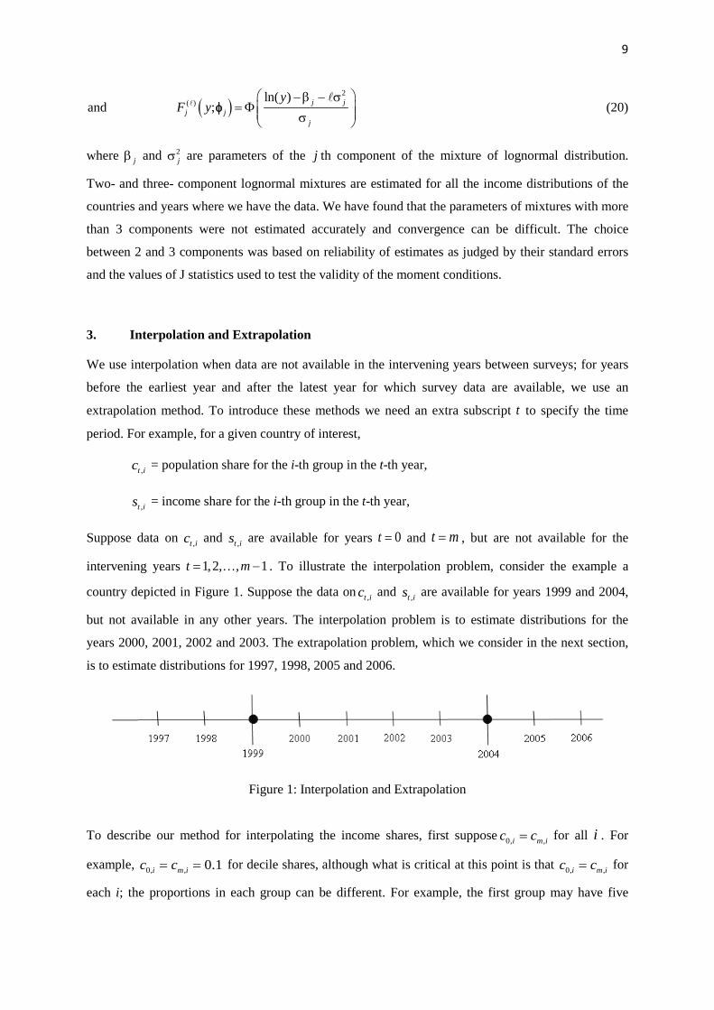
intervening years 1,2, , 1t m= − . To illustrate the interpolation problem, consider the example a

country depicted in Figure 1. Suppose the data on ,t ic and ,t is are available for years 1999 and 2004,

but not available in any other years. The interpolation problem is to estimate distributions for the

years 2000, 2001, 2002 and 2003. The extrapolation problem, which we consider in the next section,

is to estimate distributions for 1997, 1998, 2005 and 2006.

Figure 1: Interpolation and Extrapolation

To describe our method for interpolating the income shares, first suppose 0, ,i m ic c= for all i . For

example, 0, , 0.1i m ic c= = for decile shares, although what is critical at this point is that 0, ,i m ic c= for

each i; the proportions in each group can be different. For example, the first group may have five

10

percent of the population whereas the second group may have 10 percent of the population and so on.

We assume that the change in the income shares for each income class for the intervention years is

proportional to the total change in the income shares for the same income class between years 0t =

and t m= . Interpolation is carried out by interpolating the income shares as follows:

( ), 0, , 0,00t i i m i i

ts s s sm− = + − −

(21)

It can be see that the right hand side is a weighted average of the observed shares in period 0 and m.

Further, to be able to proceed with GMM estimation of the mixture of lognormal distributions

suggested by Griffiths and Hajargasht (2012), we set up the data on class means ,t iy and the quantity

,t iy where ,,

,

t i tt i

t i

s yy

c= and , ,i t i t iy c y= , where ty is the country total mean income for the year t. Then

these ,t iy are used along with proportions ,t ic to find GMM-estimated lognormal mixture

distributions for the years 1,2, , 1t m= − .

The above method for calculating the ,t is assumes 0, ,i m ic c= . If this equality does not hold we must

find a new set of population proportions ,m ic∗ such that , ,m i o ic c∗ = , and then find income shares ,m is∗ that

correspond to the population proportions ,m ic∗ . To do this we would need to invert the estimated

distribution function at year m to find corresponding quantiles, and then find income shares for these

quantiles using the first moment distribution function specified in equation (15). The values of *,m is

are used to replace ,m is in equation (21).

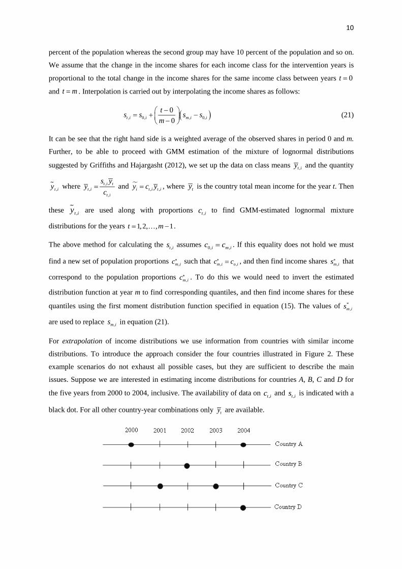
For extrapolation of income distributions we use information from countries with similar income

distributions. To introduce the approach consider the four countries illustrated in Figure 2. These

example scenarios do not exhaust all possible cases, but they are sufficient to describe the main

issues. Suppose we are interested in estimating income distributions for countries A, B, C and D for

the five years from 2000 to 2004, inclusive. The availability of data on ,t ic and ,t is is indicated with a

black dot. For all other country-year combinations only ty are available.

11

Figure 2: Examples of where extrapolation is required

A general description of how we can proceed follows.

1. Current-price income distributions are estimated for all countries-year combinations

where there are black dots.

2. The interpolation method is used to estimate distributions for

country A: 2001, 2002, 2003

country C: 2002

3. We compute weights that reflect the “distance” or “similarity” between the income

distributions (A, 2002) and (B, 2002) and between distributions (C, 2002) and (B, 2002).

Possible distance/similarity measures are described below.

4. For estimating distributions for (B, 2001) and (B, 2003), we assume that changes in the

income shares for these country-year combinations are proportional to a weighted average

of the proportional changes observed for countries A and C. The change is measured

relative to 2002 where estimated distributions are available for all three countries A, B, C.

The weights are obtained from step 3. The extrapolated income shares are given by:

( )0

1, , , 1, ,1

M

j t i j t i j k k t i k t ik

s s w s s+ +=

= + −∑ (22)

where subscript j refers to the country of interest. Countries 01,2, ,k M= are those

whose income shares are known, either because the original data are available or because

they have been interpolated. Further, the corresponding class mean income is obtained

from

1,1, 1

,

j t ij t i j t

t i

sy y

c+

+ += (23)

5. To obtain distributions for (C, 2000) and (C, 2004) we follow the same procedure as that

in step 4, but we use only the proportional changes in A from 2003 to 2004 and from 2001

to 2000. No information is available from other countries.

6. Repeat step 4 to obtain distributions for (B, 2000) and (B, 2004). Note that information

from (C, 2000) and (C, 2004), obtained in step 5, can be used in this process.

7. Obtain distributions for (D, 2000), (D, 2001), (D, 2002), and (D, 2003) using income

shares obtained as weighted averages of proportional changes for countries A, B and C.

12

8. The results from the above procedure will not be invariant with respect to the order in

which the countries are considered. For example, instead of finding (C, 2000) and (C,

2004) before (B, 2000) and (B, 2004), we could have reversed this order, using

information from only A to find (B, 2000) and (B, 2004) and then using information from

A and B to find (C, 2000) and (C, 2004). To overcome this problem we can use an

iterative scheme where information from all available sources is used. Iterating until

convergence is likely to be too demanding, but one or two iterations is likely to improve

the consistency of the results. A matrix equation involving all countries where

extrapolation is required can be set up to compute these iterations.

The missing piece from the above steps is how to measure the distance or similarity between two

distributions. To do so, we use a normalized version of Kullback-Leibler (KL) distance (Kullback and

Leibler, 1951). Let ( )A Af y µ and ( )B Bf y µ be normalized income distributions for countries A and

B, respectively in a given year. Then, the KL divergence of Bf from Af is

( ) ( )( ) ( ) ( )

0

ln A AA A A

B B

f yKL A B f y d y

f y

∞

µ= µ µ µ

⌠⌡

As a symmetric measure of distance from A to B we use

( ) ( )( ),12A BD KL A B KL B A= +

when ( ) ( )A A B Bf y f yµ = µ , , 0A BD = . Suppose, we consider the distances of country A from a

number of other countries 1,2, ,j J= . Then, for weights which reflect the closeness of A to each

of these countries, we use 1 1, , ,

1

J

A j A j A ll

w D D− −

=

= ∑ . To compute 1,A jD− we need to take expectations of

the log of mixtures of lognormal distributions, which we do numerically.

4. Combining Country level Distributions

Once distributions have been estimated for every country/year combination, we can find the regional

distribution for Africa as a population-weighted mixture of the country-level distributions as

described by Chotikapanich et al (2007). Since the country-level distributions are estimated as

lognormal mixtures, the regional distributions are essentially mixtures of mixtures.

The density function for the income distribution of a region is given by the mixture

1( ) ( )Kk kkf y f y== λ∑ where 1 2, , Kλ λ λ are the population proportions for each country.

13

The regional cdf is given by1

( ) ( )K

k kk

F y F y=

= λ∑ and the regional mean income is given by

1

K

k kk=

µ = λ µ∑ .

5. Measures of Inequality and Poverty for Mixtures of Lognormal distributions

The main purpose of compiling a panel of income distributions is to assess welfare changes over time

using various definitions of welfare that take into account inequality, poverty, mean income, and

whether growth has favoured the poor. Various measures for these concepts have appeared in the

literature, and typically depend on characteristics of the income distribution. To compute values of

these measures we express them in terms of the parameters of a mixture of lognormal distributions.

Inequality measures that will be considered include the Gini coefficient (G), and Theil’s measure (T)3.

The expressions for these measures in terms of the parameters of the mixture of lognormal

distributions are:

( )

( )

22

2 21 1

2

1

2 exp 0.5

1exp 0.5

n ni i j

i j i ii j i j

n

j j jj

w w

Gw

= =

=

σ +β −β β + σ Φ σ + σ = −β + σ

∑∑

∑ (24)

and,

( )2

1 1ln exp 0.5

n n

j j j j jj j

T w w= =

= β + σ − β

∑ ∑ (25)

where ( ) 2, , 1,2, ,j j j nβ σ = are the parameters of the lognormal mixture.

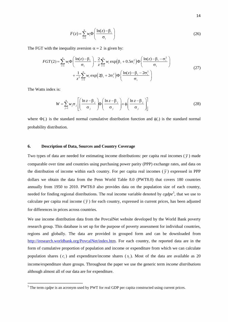
Poverty measures include the head-count ratio, the poverty gap ratio, the Foster-Greer-Thorbecke

index (FGT) and the Watts index4. The expressions for these measures in terms of the parameters of

the lognormal mixture are given below.

The headcount ratio which gives the proportion of population whose income is below the poverty line,

z is given by

3 Details of these inequality measures and expressions for them in terms of parameters of different distributions that are not mixtures can be found in, for example, Kleiber and Kotz (2003), Jenkins (2009) and McDonald and Ransom (2008). 4 See Kakwani (1999) for review of various poverty measures and Chotikapanich et al (2013) for their expressions in terms of parameters of a generalized beta distribution.

14

1

ln( )( )n

ii

i i

zF z w=

−β= Φ σ ∑ (26)

The FGT with the inequality aversion 2α = is given by:

( )

( )

22

1 1

22

21

ln( ) ln( )2(2 exp 0.5

ln( ) 21 exp 2 2

n ni i i

i i i ii ii i

ni i

i i ii i

z zFGT w wz

zwz

= =

=

−β −β − σ) = Φ − β + σ Φ σ σ

−β − σ+ β + σ Φ σ

∑ ∑

∑ (27)

The Watts index is:

1

ln ln lnnj j j

j jj j j j

z z zW w

=

−β −β −β= σ Φ + φ σ σ σ ∑ (28)

where (.)Φ is the standard normal cumulative distribution function and (.)φ is the standard normal

probability distribution.

6. Description of Data, Sources and Country Coverage

Two types of data are needed for estimating income distributions: per capita real incomes ( y ) made

comparable over time and countries using purchasing power parity (PPP) exchange rates, and data on

the distribution of income within each country. For per capita real incomes ( y ) expressed in PPP

dollars we obtain the data from the Penn World Table 8.0 (PWT8.0) that covers 180 countries

annually from 1950 to 2010. PWT8.0 also provides data on the population size of each country,

needed for finding regional distributions. The real income variable denoted by cgdpe5, that we use to

calculate per capita real income ( y ) for each country, expressed in current prices, has been adjusted

for differences in prices across countries.

We use income distribution data from the PovcalNet website developed by the World Bank poverty

research group. This database is set up for the purpose of poverty assessment for individual countries,

regions and globally. The data are provided in grouped form and can be downloaded from

http://iresearch.worldbank.org/PovcalNet/index.htm. For each country, the reported data are in the

form of cumulative proportion of population and income or expenditure from which we can calculate

population shares ( ic ) and expenditure/income shares ( is ). Most of the data are available as 20

income/expenditure share groups. Throughout the paper we use the generic term income distributions

although almost all of our data are for expenditure.

5 The term cgdpe is an acronym used by PWT for real GDP per capita constructed using current prices.

15

Regarding the data coverage, we began with as many countries in Africa as possible where we have

the data on both per capita real incomes and the corresponding income distributions. Our data set

include 40 countries with the data scatter between 1993 and 2011. These countries are mostly in Sub-

Saharan Africa and they cover most of the countries in the Sub-Saharan Africa. For each country, the

number of years where the data are available range between 1 and 5 years. These countries and the

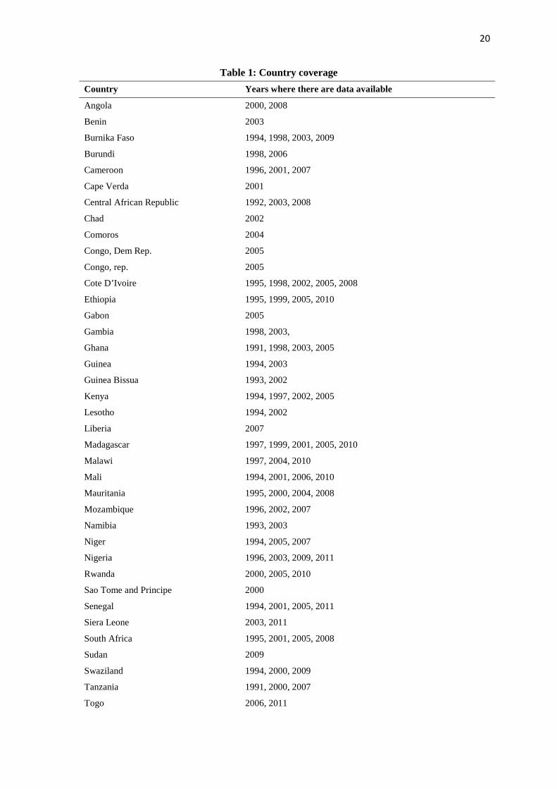
years where the data are available are listed in Table 1.

(Table 1 here)

7. Empirical Results

The main objective of the paper is to compile a panel of income distributions for 40 Sub-Saharan

African countries and for the period 1993 to 2011. As a first step in this process, we first fit mixture of

lognormal distributions using GMM discussed in Section 2. Considering the limitations of space, we

focus our presentation to a subset of ten countries. These are: Central African Republic; Ethiopia;

Ghana; Kenya; Mozambique; Nigeria; Senegal; Sierra Leone; South Africa and Tanzania.

Table 2 presents the estimated parameters of the mixtures of lognormal distributions for the 10

countries. For example, consider the fitted distribution for Ethiopia in 1997 from Table 2. Column 2

indicates whether the estimates were obtained from observed data (O), interpolated data (I) or

extrapolated data (E).; Column 3 indicates the form of the best fitting distribution and the remaining

columns show the estimated parameters. In the case of Ethiopia, the best fitting distribution is a

mixture of two lognormal distributions with both variances estimates which is indicated by (2,2).6 In

the case of Ethiopia, noting that for a random variable 2 2( , ) ln ( , )X LN X Nµ σ ⇔ µ σ where

LN and N denote lognormal and normal distributions, the parameters estimated for Ethiopia are:

1µ =5.759; σ1 = 0.0468; weight1 = 0.904 and µ2 =6.575; σ2 = 0.871; weight2 = 0.096

This means that the first distribution has 90% weight compared to 10% for the second distribution and

hence the first distribution is the main driver of the distribution.

(Table 2: Fitted Distributions for 10 African countries and for Selected Years)

A feature worth noting in Table is the stability of the fitted distributions over time. There are no major

shifts in the number of distributions involved in the mixture nor are there major changes in the

weights accorded to the distributions in the mixture. This stability is an encouraging feature which

provides a basis for interpolation and extrapolation of distributions based on the observed

distributions.

6 If the column shows (3,2) then it means that the fitted distribution is a mixture of three lognormal distributions but only two variances are estimated. This means that the last two components of the mixture have the same variance parameter.

16

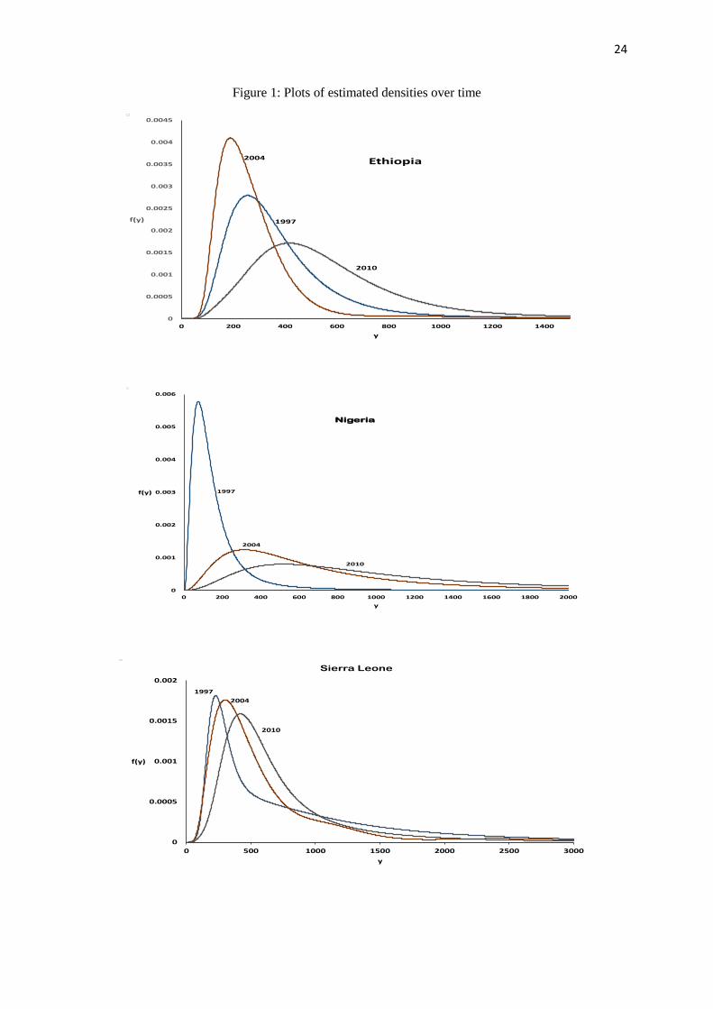
The following figures show the estimated densities for the years 1997, 2004 and 2010 for Ethiopia,

Nigeria and Sierra Leone.

(insert Figure 1 here)

Fitted distributions for Nigeria and Sierra Leone are consistent with expectations showing a rightward

shift in the distributions. In the case of Nigeria, the profile of distributions suggests a strong growth in

real per capita income and also a significant reduction in inequality. The case of Ethiopia is somewhat

puzzling as the distribution in 2004 shifted to the left of the distribution in 1997 indicating a

significant drop in real per capita income and then an expected rightward shift in the distribution for

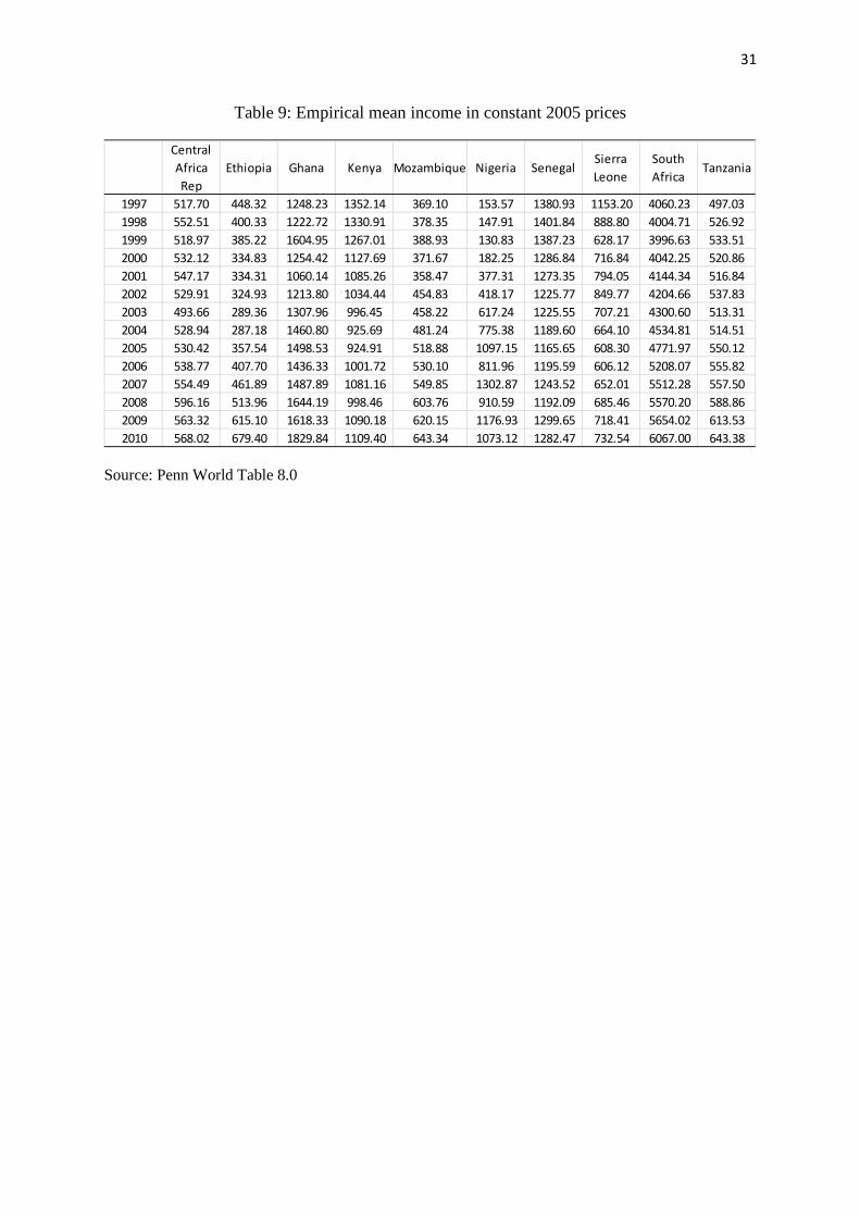
2010. This could be partly driven by the data on real per capita income from the Penn World Tables

(PWT 8.0). From Table 9, it can be seen that real per capita income in constant 2005 prices has

dropped from $448.32 in 1997 to $287.18 in 2004. This drop in mean income implies a shift of the

distribution in 2004 to the left of the distribution in 1997.

Interpolation and extrapolation of income distribution data

Table 3 shows the current availability of data for the ten countries under consideration. All the entries

coloured in yellow shows the current availability of income distribution data. Income distribution data

are indeed sparse with only 21 entries out of possible 240 (10 countries by 14 years) in yellow

showing availability. This means that we need to interpolate or extrapolate using data available. As

discussed in Section 3, income distributions are interpolated for all the years in between the years

when data are available, i.e., for all the years between yellow coloured squares (these are the squares

in green). We need to extrapolate the distributions for all the light organge coloured squares. There

are 21 entries (countries and years) for which extrapolations are made. Our methodology for

interpolation is quite simple as it interpolates the income shares for the decile or quintile groups but

extrapolation requires the computation of Kullback-Leibler measures of distance7 between pairs of

income distributions. The weights implied are presented in Table 4.

(Table 4 here)

The table shows the years for which extrapolations are made and the weights attached to the

distributions from different countries. For example, consider the first row of the table. This

corresponds to the extrapolation of income distribution for Central African Republic in 2009. This

distribution is derived as a weighted average of the distributions from Ethiopia, Ghana, Kenya,

Mozambique, Nigeria, Senegal, Sierra Leone, South Africa and Tanzania. Of these countries, the

biggest weight of 0.22 is for the distribution of Sierra Leone followed by Ghana with a weight of

0.166 and Kenya with a weight of 0.147. The lowest weight is given to the distribution from Ethiopia.

7 The matrix of Kullback-Leibler distances is computed for all the 40 countries in the study but only relevant parts of the distance matrix are used in this paper.

17

These weights suggest that the usual naïve approach of using the distribution of the geographically

closest neighbour may not be the best approach to be used.

Using the procedures described in Section 3, we compile the full set of 240 income distribution based

on the observed, interpolated or extrapolated income distributions. These distributions are used in

assessing the inequality and poverty situation in the selected 10 African countries over the period

1997 to 2010.

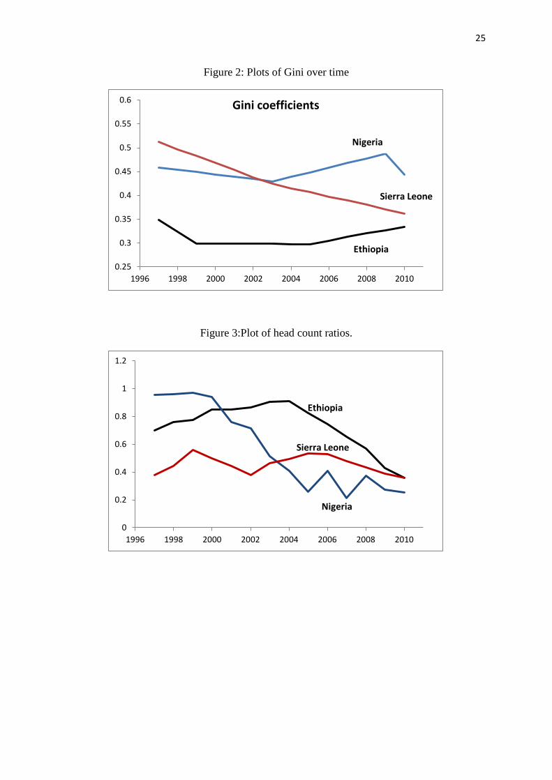
Inequality and poverty

In tables 5 and 6 we present the estimated Gini and Theil’s measures of inequalities for the 10

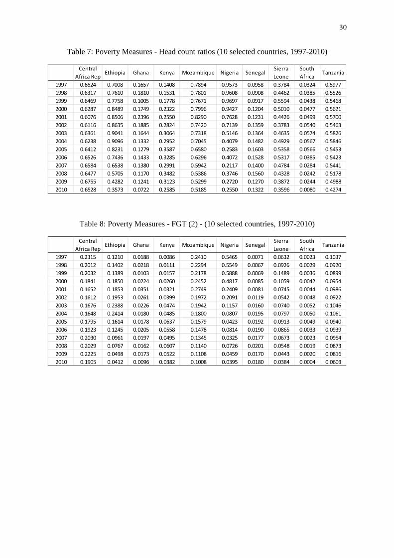
selected countries. Tables 7 and 8 present the head count ratio and Foster-Greer-Thorbecke index with

parameter value of 2 (FGT(2)).

We observe increase in inequality over the period 1997 to 2010 in Central African Republic, Ghana,

Kenya, South Africa and Tanzania whereas marginal decrease in inequality is observed in other

countries of the region. Of particular relevance is the increase in inequality in South Africa, Ghana

and Kenya. The time profiles of inequality measures are shown in Figure 2 for Nigeria, Ethiopia and

Sierra Leone.

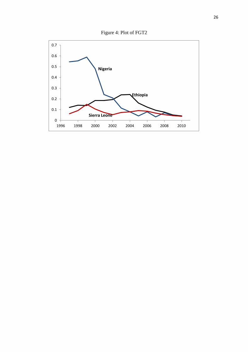
However, no such simple profile can be observed for poverty measures. As poverty measures are

determined by real per capita income as well as inequality in the distribution of income, we observe

significant fluctuations in head count ratio as well as FGT (2) for Nigeria, Ethiopia and Sierra Leone.

These fluctuations can be largely attributable to fluctuations in real per capita income shown in Table

9.

8. Conclusions

We have shown how estimation, interpolation and extrapolation can be used to construct a panel of

income distributions for a subset of African countries. This panel can be used to analyse changes in

poverty, inequality and other measures of interest. The paper is part of a larger study which will

eventually include many more countries.

18

References

African Development Bank (2012), Briefing Notes for AfDB’s Long Term Strategy, Briefing Note 5: Income Inequality in Africa.

Anderson G., O. Linton and Y.-J. Whang (2012), “Nonparametric estimation and Inference about the overlap of two distributions,” Journal of Econometrics, 171, 1-23.

Atkinson, A. B., & Brandolini, A. (2001). Promise and Pitfalls in the Use of "Secondary" Data-Sets: Income Inequality in OECD Countries as a Case Study. Journal of Economic Literature, 39(3), 771-799.

Bhalla, S. S. (2002). Imagine There's No Country: Poverty, Inequality, and Growth in the Era of Globalization. Washington, D.C: Institute for International Economics.

Bhalla, S. S. (2004), “Poor Results and Poor Policy: A Comparative Analysis of Estimates of Global Inequality and Poverty,” CESifo Economic Studies 50:1, 85-132.

Chen, S. and M. Ravallion (2010), “The Developing World is Poorer than We Thought, But No Less Successful in the Flight Against Poverty,” The Quarterly Journal of Economics, 125, 1577-1625.

Chotikapanich, D., W.E. Griffiths, and D.S.P. Rao (2007), “Estimating and Combining National Income Distributions using Limited Data”, Journal of Business and Economic Statistics, 25, 97-109.

Chotikapanich, D., W.E. Griffiths, D. S. Prasada Rao, and V. Valencia (2012) “Global Income Distributions and Inequality, 1993 and 2000: Incorporating Country-Level Inequality Modelled with Beta Distributions,” Review of Economics and Statistics, 94, 52-73.

Chotikapanich, D., W.E. Griffiths, W. Karunarathne and D.S.P. Rao (2013), “Calculating Poverty Measures from the Generalized Beta Income Distribution,” Economic Record, 89, S1, 48-66.

Deininger, K., & Squire, L. (1996). A new data set measuring income inequality. World Bank Economic Review, 10(3), 565-591.

Dowrick, Steve and Muhammad Akmal (2005), “Contradictory Trends in Global Income Inequality: A Tale of Two Biases,” Review of Income and Wealth 51:2, 201-229.

Feenstra, R.C., R. Inklaar, and M. Timmer (2013), “The Next Generation of the Penn World Table,” NBER Working Papers 17916, National Bureau of Economic Research, Inc.

Griffiths, W.E. and R. Hajargasht (2012), “GMM Estimation of Mixtures from Grouped Data: An application to Income Distributions,” Department of Economics Working Papers 1148, Melbourne University

Grimm, M. (2007), “Removing the Anonymity in Assessing Pro-poor Growth,” Journal of Economic Inequality, 5, 179-197.

Hajargasht, G., W.E. Griffiths, J. Brice, D.S.P. Rao and D. Chotikapanich (2012), “Inference for Income Distributions using Grouped Data,” Journal of Business and Economic Statistics, 30, 563-575.

Heston, A., Summers, R., & Aten, B. (2009). Penn World Table Version 6.3. Center for International Comparisons of Production, Income and Prices. University of Pennsylvania: August 2009.

Kleiber, Christian and Samuel Kotz, Statistical Size Distributions in Economics and Actuarial Sciences, (New York: John Wiley and Sons, 2003).

Kullback, S., and R.A. Liebler (1951), “On Information and Sufficiency,” Annals of Mathematical Statistics, 22, 79-86.

Lambert, P.J. (2010), “Pro-poor Growth and the lognormal Income Distribution,” Journal of Income Distribution, 19, 88-99.

19

McDonald, James. B. and Michael R. Ransom (2008), “The Generalized Beta Distribution as a Model for the Distribution of Income: Estimation of Related Measures of Inequality,” (pp. 147-166), in Duangkamon Chotikapanich (Ed.), Modeling Income Distributions and Lorenz Curves (New York: Springer, 2008).

Milanovic, Branko (2002), “True World Income Distribution, 1988 and 1993: First Calculations based on Household Surveys Alone," The Economic Journal, 112, 51-92.

Milanovic, Branko (2005), Worlds Apart: measuring International and Global Inequality, New Jersey: Princeton University Press.

Milanovic, B. (2009). Global Inequality Recalculated: The Effect of new 2005 PPP estimates on Global Inequality. MPRA Working Paper No. 16535, University of Munich.

Pinkovskiy, M. and Xavier Sala-i-Martin (2009), “Parametric Estimations of the World Distribution of Income,” NBER Working Papers 15433, National Bureau of Economic Research, Inc.

Rao D.S.P., A. Rambaldi and H. Doran (2010), “Extrapolation of Purchasing Power Parities using Multiple Benchmarks and Auxiliary Information: A New Approach”, Review of Income and Wealth, Special Issue. Series 56, Special Issue 1, June, 2010, pp. S59-S98.

Ravallion, M. and S. Chen, (2003), "Measuring Pro-poor Growth," Economics Letters, 78(1), 93-99.

Sala-i-Martin, Xavier (2006), “The World Distribution of Income: Falling Poverty and ….Convergence, Period”, The Quarterly Journal of Economics 121:2 , 351-397.

Sen, Amartya K (1976), “Real National Income,” Review of Economic Study, 43, 19-39

Summers, R, and A. Heston (1991), “The Penn World Table (Mark 5): An Expanded Set of International Comparisons, 1950-1988,” The Quarterly Journal of Economics, 106, 327-368.

Theil, H. (1979). World income inequality and its components. Economics Letters, 2(1), 99-102.

Warner, D., D.S.P. Rao, W.E. Griffiths, Duangkamon Chotikapanich (2014), “Global Inequality: Levels and Trends, 1993-2005 How sensitive are these to the choice of PPPs and Real Income measures,” Accepted for publication in the Review of Income and Wealth, July, 2014.

UNU-WIDER (2008). World Income Inequality Database, Version 2.0c. Retrieved February 18, 2009, from http://www.wider.unu.edu/research/Database/en_GB/wiid/.

20

Table 1: Country coverage Country Years where there are data available

Angola 2000, 2008

Benin 2003

Burnika Faso 1994, 1998, 2003, 2009

Burundi 1998, 2006

Cameroon 1996, 2001, 2007

Cape Verda 2001

Central African Republic 1992, 2003, 2008

Chad 2002

Comoros 2004

Congo, Dem Rep. 2005

Congo, rep. 2005

Cote D’Ivoire 1995, 1998, 2002, 2005, 2008

Ethiopia 1995, 1999, 2005, 2010

Gabon 2005

Gambia 1998, 2003,

Ghana 1991, 1998, 2003, 2005

Guinea 1994, 2003

Guinea Bissua 1993, 2002

Kenya 1994, 1997, 2002, 2005

Lesotho 1994, 2002

Liberia 2007

Madagascar 1997, 1999, 2001, 2005, 2010

Malawi 1997, 2004, 2010

Mali 1994, 2001, 2006, 2010

Mauritania 1995, 2000, 2004, 2008

Mozambique 1996, 2002, 2007

Namibia 1993, 2003

Niger 1994, 2005, 2007

Nigeria 1996, 2003, 2009, 2011

Rwanda 2000, 2005, 2010

Sao Tome and Principe 2000

Senegal 1994, 2001, 2005, 2011

Siera Leone 2003, 2011

South Africa 1995, 2001, 2005, 2008

Sudan 2009

Swaziland 1994, 2000, 2009

Tanzania 1991, 2000, 2007

Togo 2006, 2011

21

Uganda 1996, 1999, 2002, 2005, 2009

Zambia 1996, 1998, 2002, 2004, 2006, 2010

Source: PovalNet as of June, 2014 at http://iresearch.worldbank.org/PovcalNet/index.htm

22

Table 2: Fitted Distributions for 10 Selected African Countries, 1997, 2004, 2010

Country Year Data Model mu1 sig1 w1 mu2 sig2 w2 mu3 sig3 w3Central African Republic 1997 I 3,2 5.4572 0.8121 0.8290 6.5477 0.3101 0.1011 7.7046 0.3101 0.0699Central African Republic 1998 I 3,2 5.5480 0.7780 0.8258 6.5776 0.2964 0.1005 7.6999 0.2964 0.0737Central African Republic 1999 I 3,2 5.5305 0.7498 0.8260 6.4983 0.2790 0.0974 7.5890 0.2790 0.0766Central African Republic 2000 I 3,2 5.6105 0.7269 0.8307 6.5136 0.2540 0.0906 7.5760 0.2540 0.0787Central African Republic 2001 I 3,2 5.6868 0.7061 0.8337 6.5333 0.2424 0.0874 7.5676 0.2424 0.0789Central African Republic 2002 I 3,2 5.7122 0.6941 0.8523 6.4851 0.1907 0.0702 7.4995 0.1907 0.0776Central African Republic 2003 O 3,2 5.3011 0.5584 0.4364 6.1556 0.5423 0.4914 7.2166 0.5423 0.0722Central African Republic 2004 I 3,2 4.8313 0.2249 0.0254 5.8409 0.7412 0.9264 7.3281 0.7412 0.0482Central African Republic 2005 I 3,2 4.7579 0.2135 0.0217 5.8205 0.7705 0.9420 7.6301 0.7705 0.0362Central African Republic 2006 I 3,2 4.6659 0.2088 0.0181 5.7768 0.8007 0.9507 7.8383 0.8007 0.0313Central African Republic 2007 I 3,2 4.5821 0.2047 0.0139 5.7420 0.8351 0.9582 8.0265 0.8351 0.0278Central African Republic 2008 O 3,2 4.3996 0.5002 0.0580 5.7872 0.8000 0.9010 8.0063 0.8000 0.0410Central African Republic 2009 E 2,2 5.6502 0.8692 0.9295 6.9368 1.3174 0.0705Central African Republic 2010 E 2,2 5.7373 0.7706 0.8597 6.2770 1.3980 0.1403Ethiopia 1997 I 2,2 5.7595 0.4680 0.9036 6.5754 0.8708 0.0964Ethiopia 1998 I 2,2 5.6459 0.4400 0.8778 6.2434 0.8376 0.1222Ethiopia 1999 O 2,2 5.6596 0.4117 0.8407 6.0778 0.7728 0.1593Ethiopia 2000 I 2,2 5.5603 0.4153 0.8631 6.0505 0.7690 0.1369Ethiopia 2001 I 2,2 5.5723 0.4185 0.8846 6.1551 0.7587 0.1154Ethiopia 2002 I 2,2 5.5581 0.4235 0.9210 6.3943 0.6937 0.0790Ethiopia 2003 I 3,2 5.0846 0.1190 0.0309 5.4842 0.4322 0.9345 6.8920 0.4322 0.0346Ethiopia 2004 I 3,2 5.2714 0.3517 0.5861 5.7737 0.3142 0.3713 6.8888 0.3142 0.0426Ethiopia 2005 O 3,2 5.4353 0.3314 0.5225 5.9552 0.3093 0.4333 7.0886 0.3093 0.0442Ethiopia 2006 I 2,2 5.7730 0.4339 0.9386 6.8150 0.6409 0.0614Ethiopia 2007 I 2,2 5.8726 0.4427 0.8901 6.4960 0.7873 0.1099Ethiopia 2008 I 3,1 5.4673 0.4410 0.0801 6.0242 0.4410 0.8739 7.3512 0.4410 0.0460Ethiopia 2009 I 3,1 5.4834 0.4378 0.0870 6.1690 0.4378 0.8610 7.4610 0.4378 0.0519Ethiopia 2010 O 3,1 5.4142 0.4424 0.0749 6.2554 0.4424 0.8689 7.5364 0.4424 0.0561Ghana 1997 I 3,2 6.6785 0.6732 0.8893 7.5116 0.2780 0.0779 8.3808 0.2780 0.0329Ghana 1998 O 3,2 6.6619 0.6855 0.8812 7.5172 0.2746 0.0858 8.3663 0.2746 0.0329Ghana 1999 I 3,2 6.8889 0.7077 0.9156 7.7049 0.2629 0.0588 8.6221 0.2629 0.0256Ghana 2000 I 3,2 6.7463 0.7450 0.9782 7.3743 0.1106 0.0134 8.6570 0.1106 0.0084Ghana 2001 I 3,1 6.1337 0.6863 0.1954 6.7733 0.6863 0.7740 7.9283 0.6863 0.0306Ghana 2002 I 3,1 6.0752 0.6595 0.1436 6.8882 0.6595 0.8072 8.0389 0.6595 0.0492Ghana 2003 I 3,1 5.9909 0.6434 0.1258 6.9115 0.6434 0.8177 8.1069 0.6434 0.0564Ghana 2004 I 3,1 5.9677 0.6307 0.1162 6.9719 0.6307 0.8230 8.2119 0.6307 0.0607Ghana 2005 O 3,1 5.9422 0.6305 0.1021 7.0294 0.6305 0.8402 8.3355 0.6305 0.0577Ghana 2006 E 3,1 5.9031 0.6360 0.0991 6.9934 0.6360 0.8427 8.3455 0.6360 0.0582Ghana 2007 E 3,1 5.8704 0.6495 0.0880 6.9839 0.6495 0.8567 8.3977 0.6495 0.0553Ghana 2008 E 3,1 5.9233 0.6621 0.0770 7.0593 0.6621 0.8691 8.5379 0.6621 0.0538Ghana 2009 E 3,1 5.8864 0.6731 0.0653 7.0511 0.6731 0.8809 8.5730 0.6731 0.0538Ghana 2010 E 3,1 5.7376 0.6536 0.0316 7.2055 0.6536 0.9229 8.6211 0.6536 0.0455Kenya 1997 O 3,2 6.0093 0.2837 0.1522 6.8883 0.5477 0.7840 8.3353 0.5477 0.0638Kenya 1998 I 3,2 5.9632 0.3137 0.1431 6.8385 0.5682 0.7955 8.3190 0.5682 0.0615Kenya 1999 I 3,2 5.9298 0.3570 0.1398 6.7866 0.5899 0.8020 8.3019 0.5899 0.0583Kenya 2000 I 3,2 5.8803 0.4213 0.1489 6.6927 0.6120 0.7968 8.2420 0.6120 0.0543Kenya 2001 I 3,1 6.1708 0.5657 0.5108 6.9131 0.5657 0.4442 8.3446 0.5657 0.0450Kenya 2002 I 2,2 6.4179 0.6695 0.8326 7.1894 0.9728 0.1674Kenya 2003 I 2,2 6.3957 0.6488 0.7293 6.8349 1.0468 0.2707Kenya 2004 I 2,2 6.4672 0.5764 0.7302 6.5572 1.1704 0.2698Kenya 2005 O 3,2 6.2817 1.5518 0.0853 6.2846 0.6351 0.7809 7.3702 0.6351 0.1339Kenya 2006 E 3,2 6.1212 0.4786 0.4097 6.5768 1.1320 0.3723 6.9148 0.4786 0.2180Kenya 2007 E 3,2 6.1611 0.4849 0.4250 6.6271 1.1573 0.3575 6.9735 0.4849 0.2175Kenya 2008 E 3,2 6.1070 0.4935 0.4455 6.5859 1.1850 0.3406 6.9404 0.4935 0.2139Kenya 2009 E 3,2 6.1428 0.4969 0.4581 6.6384 1.2025 0.3319 6.9946 0.4969 0.2100Kenya 2010 E 3,2 6.2039 0.4145 0.3932 6.7030 1.1192 0.3652 7.0000 0.4145 0.2416Mozambique 1997 I 3,2 5.2966 0.2025 0.0513 5.5049 0.6765 0.9073 7.3160 0.6765 0.0413Mozambique 1998 I 3,2 5.4024 0.3495 0.1298 5.5350 0.7030 0.8326 7.3860 0.7030 0.0376Mozambique 1999 I 2,2 5.4869 0.5813 0.7609 5.9960 1.0756 0.2391Mozambique 2000 I 3,2 5.3818 0.3666 0.1625 5.5040 0.7119 0.8003 7.4269 0.7119 0.0372Mozambique 2001 I 3,2 5.3401 0.3667 0.1715 5.4600 0.7143 0.7912 7.4175 0.7143 0.0373Mozambique 2002 O 3,2 5.5728 0.3821 0.1919 5.6910 0.7172 0.7702 7.6745 0.7172 0.0379Mozambique 2003 I 2,2 5.6446 0.5831 0.7681 6.1169 1.1373 0.2319Mozambique 2004 I 2,2 5.7132 0.5920 0.7706 6.1143 1.1593 0.2294Mozambique 2005 I 2,2 5.8086 0.6023 0.7785 6.1403 1.1868 0.2215Mozambique 2006 I 3,1 0.3571 0.6663 0.0062 5.8551 0.6663 0.9579 7.8299 0.6663 0.0359Mozambique 2007 O 3,1 0.0736 0.6741 0.0072 5.9045 0.6741 0.9610 7.8972 0.6741 0.0319Mozambique 2008 E 3,2 5.6443 0.4820 0.3980 6.1683 1.2252 0.2462 6.3485 0.4820 0.3558Mozambique 2009 E 3,2 5.6721 0.4864 0.4187 6.1993 1.2411 0.2422 6.3818 0.4864 0.3391Mozambique 2010 E 3,2 5.7268 0.4043 0.3633 6.2461 1.1552 0.2706 6.4454 0.4043 0.3662

23

Table 2: Fitted Distributions for 10 Selected African Countries, 1997, 2004, 2010 (cont)

Country Year Data Model mu1 sig1 w1 mu2 sig2 w2 mu3 sig3 w3Nigeria 1997 I 3,1 3.7720 0.6560 0.0674 4.8095 0.6560 0.8796 6.4628 0.6560 0.0530Nigeria 1998 I 3,1 3.9084 0.6575 0.0767 4.9238 0.6575 0.8709 6.5177 0.6575 0.0524Nigeria 1999 I 3,1 3.6689 0.6591 0.0858 4.6680 0.6591 0.8622 6.1973 0.6591 0.0520Nigeria 2000 I 3,1 3.8254 0.6606 0.0947 4.8127 0.6606 0.8533 6.2699 0.6606 0.0520Nigeria 2001 I 3,1 4.6363 0.6620 0.1032 5.6157 0.6620 0.8442 6.9904 0.6620 0.0527Nigeria 2002 I 3,1 4.7746 0.6628 0.1111 5.7494 0.6628 0.8338 7.0256 0.6628 0.0551Nigeria 2003 O 3,2 4.5683 0.4256 0.0267 6.1127 0.7103 0.9253 7.3119 0.7103 0.0480Nigeria 2004 I 2,2 6.2905 0.6728 0.5676 6.3610 0.9532 0.4324Nigeria 2005 I 2,2 6.6005 0.6996 0.6529 6.7391 0.9997 0.3471Nigeria 2006 I 2,2 6.2686 0.7110 0.6749 6.4729 1.0237 0.3251Nigeria 2007 I 2,2 6.7491 0.7182 0.6797 7.0162 1.0388 0.3203Nigeria 2008 I 2,2 6.4667 0.7235 0.6778 6.7942 1.0494 0.3222Nigeria 2009 O 2,2 6.7175 0.7216 0.6552 7.0985 1.0521 0.3448Nigeria 2010 I 2,2 6.7162 0.6415 0.5948 6.9099 0.9718 0.4052Senegal 1997 I 3,2 6.4090 0.0188 0.0213 6.7861 0.5708 0.8967 8.2230 0.5708 0.0820Senegal 1998 I 3,2 6.4142 0.0718 0.0245 6.8042 0.5722 0.8951 8.2424 0.5722 0.0804Senegal 1999 I 3,2 6.3762 0.1363 0.0382 6.7962 0.5795 0.8884 8.2503 0.5795 0.0734Senegal 2000 I 3,2 6.6186 0.5160 0.8231 7.3785 0.2527 0.0974 8.3636 0.2527 0.0795Senegal 2001 O 3,2 6.5445 0.4766 0.7413 7.2879 0.2689 0.1674 8.3006 0.2689 0.0914Senegal 2002 I 3,2 6.3136 0.2114 0.0704 6.7765 0.6322 0.8989 8.4580 0.6322 0.0307Senegal 2003 I 3,2 0.2262 4.2529 0.0085 6.4947 0.4693 0.6402 7.3727 0.4693 0.3512Senegal 2004 I 3,2 0.2601 4.1408 0.0114 6.4770 0.4696 0.6105 7.3457 0.4696 0.3781Senegal 2005 O 3,2 6.5876 1.3423 0.0612 6.5916 0.5456 0.6764 7.3720 0.5456 0.2624Senegal 2006 I 3,1 0.2628 0.6220 0.0048 6.7413 0.6220 0.9123 7.8332 0.6220 0.0829Senegal 2007 I 3,1 0.2328 0.6117 0.0054 6.7473 0.6117 0.8905 7.8086 0.6117 0.1041Senegal 2008 I 3,1 0.2016 0.6028 0.0061 6.7387 0.6028 0.8731 7.7914 0.6028 0.1208Senegal 2009 I 3,1 0.1770 0.5950 0.0067 6.7653 0.5950 0.8596 7.8206 0.5950 0.1337Senegal 2010 I 3,1 0.1478 0.5883 0.0073 6.7339 0.5883 0.8492 7.7977 0.5883 0.1435Sierra Leone 1997 I 2,2 5.5134 0.3470 0.2940 6.8162 0.8335 0.7060Sierra Leone 1998 I 3,2 5.4885 0.4232 0.4636 6.6677 0.4468 0.4130 7.7454 0.4468 0.1234Sierra Leone 1999 I 3,2 5.3507 0.1639 0.1424 5.3568 0.8602 0.0745 6.2362 0.8602 0.7831Sierra Leone 2000 I 3,2 5.4274 0.1660 0.1085 5.8855 0.7451 0.6355 6.7914 0.7451 0.2560Sierra Leone 2001 I 3,2 5.6012 0.1700 0.0730 5.9687 0.6614 0.7064 7.0651 0.6614 0.2206Sierra Leone 2002 I 2,2 5.9953 0.5631 0.7586 7.1649 0.6059 0.2414Sierra Leone 2003 O 2,2 6.0452 0.5721 0.8490 7.3457 0.5311 0.1510Sierra Leone 2004 I 3,2 6.0226 0.5652 0.8777 7.0846 0.2021 0.0669 7.8420 0.2021 0.0554Sierra Leone 2005 I 2,2 5.9566 0.5475 0.8516 7.1875 0.5322 0.1484Sierra Leone 2006 I 3,2 5.9807 0.5406 0.8810 6.9714 0.1936 0.0638 7.7327 0.1936 0.0552Sierra Leone 2007 I 2,2 5.9562 0.4116 0.4434 6.4199 0.7557 0.5566Sierra Leone 2008 I 3,2 6.0499 0.4113 0.4794 6.0513 0.7190 0.0905 6.6042 0.7190 0.4301Sierra Leone 2009 I 2,2 6.1250 0.4004 0.4686 6.5456 0.7339 0.5314Sierra Leone 2010 I 2,2 6.1913 0.3981 0.4892 6.5907 0.7256 0.5108South Africa 1997 I 3,2 7.0217 0.6046 0.4584 7.8660 0.6645 0.3658 9.2132 0.6645 0.1759South Africa 1998 I 3,2 7.0337 0.6287 0.5186 7.9510 0.6428 0.3097 9.2342 0.6428 0.1717South Africa 1999 I 3,2 7.0628 0.6548 0.5663 8.0367 0.6237 0.2644 9.2660 0.6237 0.1692South Africa 2000 I 3,2 7.1149 0.6859 0.6168 8.1510 0.6020 0.2184 9.3189 0.6020 0.1648South Africa 2001 O 3,2 7.0550 0.6729 0.5708 8.0279 0.6696 0.2641 9.3302 0.6696 0.1651South Africa 2002 I 3,2 7.0052 0.6689 0.5460 7.9104 0.7299 0.2899 9.3281 0.7299 0.1642South Africa 2003 I 3,2 7.0332 0.6763 0.6167 8.0681 0.7591 0.2395 9.4352 0.7591 0.1438South Africa 2004 I 3,2 7.0466 0.6746 0.6521 8.1930 0.7888 0.2188 9.5509 0.7888 0.1290South Africa 2005 O 3,2 7.0881 0.6763 0.7199 8.5811 0.7230 0.1916 9.9311 0.7230 0.0885South Africa 2006 I 3,2 6.9892 0.5448 0.2721 7.5434 0.8351 0.5543 9.4979 0.8351 0.1736South Africa 2007 I 3,2 6.9638 0.4766 0.1746 7.5513 0.8027 0.6400 9.5048 0.8027 0.1854South Africa 2008 O 3,2 6.9458 0.4243 0.1276 7.5647 0.7822 0.6720 9.4757 0.7822 0.2003South Africa 2009 E 3,2 6.8842 0.3939 0.1241 7.5393 0.7843 0.6766 9.4797 0.7843 0.1994South Africa 2010 E 3,2 7.4670 0.6162 0.6904 8.7734 0.5900 0.2053 9.9679 0.5900 0.1043Tanzania 1997 I 3,2 5.9050 0.1986 0.0813 5.9856 0.6175 0.8935 6.9742 0.6175 0.0251Tanzania 1998 I 3,2 4.9866 0.3026 0.0526 6.0012 0.4795 0.8241 6.9236 0.4795 0.1234Tanzania 1999 I 3,2 5.8367 0.0391 0.0248 6.0313 0.5912 0.9349 7.0212 0.5912 0.0403Tanzania 2000 O 3,2 5.1060 0.4035 0.0645 5.9921 0.4902 0.8218 6.9220 0.4902 0.1137Tanzania 2001 I 3,2 5.7791 0.0411 0.0230 5.9885 0.5927 0.9351 7.0339 0.5927 0.0419Tanzania 2002 I 3,2 4.9229 0.3040 0.0351 5.9826 0.5186 0.8691 6.9886 0.5186 0.0957Tanzania 2003 I 2,2 5.9101 0.5130 0.5817 6.1498 0.7535 0.4183Tanzania 2004 I 2,2 5.9289 0.5195 0.6098 6.1757 0.7737 0.3902Tanzania 2005 I 2,2 5.9919 0.5254 0.6332 6.2452 0.7938 0.3668Tanzania 2006 I 2,2 5.9966 0.5308 0.6522 6.2556 0.8134 0.3478Tanzania 2007 O 2,2 6.0055 0.5345 0.6624 6.2629 0.8329 0.3376Tanzania 2008 E 2,2 6.0304 0.5395 0.6931 6.3420 0.8574 0.3069Tanzania 2009 E 2,2 6.0469 0.5392 0.6999 6.3968 0.8693 0.3001Tanzania 2010 E 2,2 6.1809 0.5006 0.6438 6.3581 0.8028 0.3562

24

Figure 1: Plots of estimated densities over time

0

0.0005

0.001

0.0015

0.002

0.0025

0.003

0.0035

0.004

0.0045

0 200 400 600 800 1000 1200 1400

f(y)

y

Ethiopia2004

1997

2010

0

0.001

0.002

0.003

0.004

0.005

0.006

0 200 400 600 800 1000 1200 1400 1600 1800 2000

f(y)

y

Nigeria

2004

2010

1997

0

0.0005

0.001

0.0015

0.002

0 500 1000 1500 2000 2500 3000

f(y)

y

Sierra Leone

2010

19972004

25

Figure 2: Plots of Gini over time

Figure 3:Plot of head count ratios.

0.25

0.3

0.35

0.4

0.45

0.5

0.55

0.6

1996 1998 2000 2002 2004 2006 2008 2010

Gini coefficients

Nigeria

Sierra Leone

Ethiopia

0

0.2

0.4

0.6

0.8

1

1.2

1996 1998 2000 2002 2004 2006 2008 2010

Sierra Leone

Nigeria

Ethiopia

26

Figure 4: Plot of FGT2

0

0.1

0.2

0.3

0.4

0.5

0.6

0.7

1996 1998 2000 2002 2004 2006 2008 2010

Nigeria

Ethiopia

Sierra Leone

27

Table 3: Years where interpolation are done and years where extrapolation are done – Selected countries, 1997-2010

1997 1998 1999 2000 2001 2002 2003 2004 2005 2006 2007 2008 2009 2010

Centra l African Republ ic

Ethiopia

Ghana

Kenya

Mozambique

Nigeria

Senegal

Siera Leone

South Africa

Tanzania

Note: Meanings of colours .

The years where there are data

The years where interpolation i s done

The years where extrapolation i s done

Table 4: Weights used for extrapolation.

Extrapolated years

Central Africa Rep

Ethiopia Ghana Kenya Mozambique Nigeria SenegalSierra Leone

South Africa

Tanzania

Central Africa 2009 0.0168 0.1658 0.1469 0.0982 0.1912 0.0746 0.2201 0.0417 0.04482010 0.0334 0.3804 0.1485 0.4378

Ghana 2006 0.06110 0.0105 0.0896 0.6270 0.0329 0.1224 0.0103 0.04632007 0.06110 0.0105 0.0896 0.6270 0.0329 0.1224 0.0103 0.04632008 0.07071 0.0121 0.7256 0.0380 0.1416 0.01192009 0.0132 0.7910 0.0414 0.15442010 0.07156 0.0123 0.7344 0.0385 0.1433

Kenya 2006 0.05226 0.0093 0.1805 0.3011 0.2122 0.0344 0.1666 0.0100 0.03372007 0.05226 0.0093 0.1805 0.3011 0.2122 0.0344 0.1666 0.0100 0.03372008 0.07856 0.0140 0.2714 0.3190 0.0517 0.2504 0.01502009 0.0154 0.2994 0.3519 0.0570 0.27632010 0.07975 0.0142 0.2755 0.3238 0.0524 0.2543

Mozambique 2008 0.05177 0.0140 0.1282 0.4464 0.1821 0.0387 0.1240 0.01472009 0.0150 0.1373 0.4782 0.1951 0.0415 0.13282010 0.05255 0.0143 0.1301 0.4531 0.1849 0.0393 0.1259

South Africa 2009 0.0378 0.1628 0.1634 0.1631 0.2021 0.0754 0.19542010 0.19561 0.0304 0.1310 0.1315 0.1312 0.1626 0.0606 0.1572

Tanzania 2008 0.06185 0.1307 0.1737 0.1309 0.1128 0.1198 0.1623 0.0912 0.01672009 0.1393 0.1852 0.1396 0.1202 0.1277 0.1730 0.0972 0.01782010 0.06185 0.1307 0.1737 0.1309 0.1128 0.1198 0.1623 0.0912 0.0167

29

Table 5: Gini coefficients for the 10 selected countries, 1997-2010

Table 6: Theil indices for 10 selected countries, 1997 - 2010

Central Africa Rep

Ethiopia Ghana Kenya Mozambique Nigeria SenegalSierra Leone

South Africa

Tanzania

1997 0.5298 0.3482 0.4039 0.4234 0.4495 0.4588 0.4115 0.5126 0.5696 0.34331998 0.5134 0.3239 0.4078 0.4301 0.4530 0.4539 0.4112 0.4959 0.5721 0.34381999 0.4971 0.2996 0.4105 0.4368 0.4564 0.4490 0.4113 0.4827 0.5745 0.34592000 0.4808 0.2992 0.4126 0.4435 0.4614 0.4441 0.4085 0.4682 0.5770 0.34602001 0.4648 0.2990 0.4164 0.4500 0.4657 0.4392 0.4078 0.4533 0.5955 0.35092002 0.4483 0.2987 0.4191 0.4566 0.4700 0.4343 0.4074 0.4376 0.6140 0.35412003 0.4359 0.2988 0.4219 0.4628 0.4664 0.4295 0.4058 0.4242 0.6325 0.35872004 0.4611 0.2979 0.4246 0.4435 0.4640 0.4388 0.3996 0.4149 0.6510 0.36292005 0.4863 0.2978 0.4275 0.4761 0.4618 0.4487 0.3926 0.4065 0.6696 0.36712006 0.5117 0.3053 0.4338 0.4823 0.4586 0.4585 0.3935 0.3973 0.6563 0.37132007 0.5373 0.3134 0.4403 0.4892 0.4558 0.4682 0.3955 0.3893 0.6428 0.37562008 0.5607 0.3201 0.4478 0.4972 0.4655 0.4778 0.3974 0.3801 0.6301 0.38302009 0.5691 0.3272 0.4537 0.5035 0.4717 0.4875 0.3994 0.3713 0.6355 0.38882010 0.5355 0.3344 0.4205 0.4710 0.4390 0.4432 0.4014 0.3624 0.6016 0.3556

Central Africa Rep

Ethiopia Ghana Kenya Mozambique Nigeria SenegalSierra Leone

South Africa

Tanzania

1997 0.5057 0.2616 0.2792 0.3409 0.4173 0.4160 0.3248 0.4671 0.6103 0.20581998 0.4704 0.2167 0.2831 0.3541 0.4321 0.4017 0.3245 0.4284 0.6117 0.20401999 0.4366 0.1757 0.2892 0.3680 0.4466 0.3875 0.3262 0.4177 0.6134 0.20842000 0.4041 0.1764 0.2961 0.3825 0.4594 0.3734 0.3004 0.3936 0.6151 0.20732001 0.3746 0.1775 0.3091 0.3944 0.4732 0.3595 0.2979 0.3681 0.6748 0.21632002 0.3443 0.1778 0.3153 0.4186 0.4873 0.3457 0.3279 0.3415 0.7387 0.22012003 0.3394 0.1745 0.3218 0.4320 0.4820 0.3336 0.9823 0.3228 0.8058 0.22932004 0.4047 0.1689 0.3284 0.4183 0.4761 0.3529 0.8218 0.3038 0.8770 0.23662005 0.4753 0.1688 0.3362 0.4934 0.4717 0.3758 0.2929 0.2971 0.9476 0.24412006 0.5531 0.1863 0.3493 0.4780 0.4456 0.3982 0.2782 0.2786 0.8943 0.25182007 0.6390 0.1960 0.3638 0.4980 0.4391 0.4205 0.2800 0.2764 0.8375 0.25972008 0.6978 0.1953 0.3811 0.5220 0.4792 0.4430 0.2823 0.2630 0.7880 0.27472009 0.7822 0.2019 0.3948 0.5409 0.4974 0.4652 0.2848 0.2512 0.8041 0.28642010 0.6846 0.2095 0.3302 0.4613 0.4179 0.3704 0.2876 0.2396 0.7044 0.2300

30

Table 7: Poverty Measures - Head count ratios (10 selected countries, 1997-2010)

Table 8: Poverty Measures - FGT (2) - (10 selected countries, 1997-2010)

Central Africa Rep

Ethiopia Ghana Kenya Mozambique Nigeria SenegalSierra Leone

South Africa

Tanzania

1997 0.6624 0.7008 0.1657 0.1408 0.7894 0.9573 0.0958 0.3784 0.0324 0.59771998 0.6317 0.7610 0.1810 0.1531 0.7801 0.9608 0.0908 0.4462 0.0385 0.55261999 0.6469 0.7758 0.1005 0.1778 0.7671 0.9697 0.0917 0.5594 0.0438 0.54682000 0.6287 0.8489 0.1749 0.2322 0.7996 0.9427 0.1204 0.5010 0.0477 0.56212001 0.6076 0.8506 0.2396 0.2550 0.8290 0.7628 0.1231 0.4426 0.0499 0.57002002 0.6116 0.8635 0.1885 0.2824 0.7420 0.7139 0.1359 0.3783 0.0540 0.54632003 0.6361 0.9041 0.1644 0.3064 0.7318 0.5146 0.1364 0.4635 0.0574 0.58262004 0.6238 0.9096 0.1332 0.2952 0.7045 0.4079 0.1482 0.4929 0.0567 0.58462005 0.6412 0.8231 0.1279 0.3587 0.6580 0.2583 0.1603 0.5358 0.0566 0.54532006 0.6526 0.7436 0.1433 0.3285 0.6296 0.4072 0.1528 0.5317 0.0385 0.54232007 0.6584 0.6538 0.1380 0.2991 0.5942 0.2117 0.1400 0.4784 0.0284 0.54412008 0.6477 0.5705 0.1170 0.3482 0.5386 0.3746 0.1560 0.4328 0.0242 0.51782009 0.6755 0.4282 0.1241 0.3123 0.5299 0.2720 0.1270 0.3872 0.0244 0.49882010 0.6528 0.3573 0.0722 0.2585 0.5185 0.2550 0.1322 0.3596 0.0080 0.4274

Central Africa Rep

Ethiopia Ghana Kenya Mozambique Nigeria SenegalSierra Leone

South Africa

Tanzania

1997 0.2315 0.1210 0.0188 0.0086 0.2410 0.5465 0.0071 0.0632 0.0023 0.10371998 0.2012 0.1402 0.0218 0.0111 0.2294 0.5549 0.0067 0.0926 0.0029 0.09201999 0.2032 0.1389 0.0103 0.0157 0.2178 0.5888 0.0069 0.1489 0.0036 0.08992000 0.1841 0.1850 0.0224 0.0260 0.2452 0.4817 0.0085 0.1059 0.0042 0.09542001 0.1652 0.1853 0.0351 0.0321 0.2749 0.2409 0.0081 0.0745 0.0044 0.09862002 0.1612 0.1953 0.0261 0.0399 0.1972 0.2091 0.0119 0.0542 0.0048 0.09222003 0.1676 0.2388 0.0226 0.0474 0.1942 0.1157 0.0160 0.0740 0.0052 0.10462004 0.1648 0.2414 0.0180 0.0485 0.1800 0.0807 0.0195 0.0797 0.0050 0.10612005 0.1795 0.1614 0.0178 0.0637 0.1579 0.0423 0.0192 0.0913 0.0049 0.09402006 0.1923 0.1245 0.0205 0.0558 0.1478 0.0814 0.0190 0.0865 0.0033 0.09392007 0.2030 0.0961 0.0197 0.0495 0.1345 0.0325 0.0177 0.0673 0.0023 0.09542008 0.2029 0.0767 0.0162 0.0607 0.1140 0.0726 0.0201 0.0548 0.0019 0.08732009 0.2225 0.0498 0.0173 0.0522 0.1108 0.0459 0.0170 0.0443 0.0020 0.08162010 0.1905 0.0412 0.0096 0.0382 0.1008 0.0395 0.0180 0.0384 0.0004 0.0603

31

Table 9: Empirical mean income in constant 2005 prices

Source: Penn World Table 8.0

Central Africa Rep

Ethiopia Ghana Kenya Mozambique Nigeria SenegalSierra Leone

South Africa

Tanzania

1997 517.70 448.32 1248.23 1352.14 369.10 153.57 1380.93 1153.20 4060.23 497.031998 552.51 400.33 1222.72 1330.91 378.35 147.91 1401.84 888.80 4004.71 526.921999 518.97 385.22 1604.95 1267.01 388.93 130.83 1387.23 628.17 3996.63 533.512000 532.12 334.83 1254.42 1127.69 371.67 182.25 1286.84 716.84 4042.25 520.862001 547.17 334.31 1060.14 1085.26 358.47 377.31 1273.35 794.05 4144.34 516.842002 529.91 324.93 1213.80 1034.44 454.83 418.17 1225.77 849.77 4204.66 537.832003 493.66 289.36 1307.96 996.45 458.22 617.24 1225.55 707.21 4300.60 513.312004 528.94 287.18 1460.80 925.69 481.24 775.38 1189.60 664.10 4534.81 514.512005 530.42 357.54 1498.53 924.91 518.88 1097.15 1165.65 608.30 4771.97 550.122006 538.77 407.70 1436.33 1001.72 530.10 811.96 1195.59 606.12 5208.07 555.822007 554.49 461.89 1487.89 1081.16 549.85 1302.87 1243.52 652.01 5512.28 557.502008 596.16 513.96 1644.19 998.46 603.76 910.59 1192.09 685.46 5570.20 588.862009 563.32 615.10 1618.33 1090.18 620.15 1176.93 1299.65 718.41 5654.02 613.532010 568.02 679.40 1829.84 1109.40 643.34 1073.12 1282.47 732.54 6067.00 643.38