poverty, inequality and human development in a … · poverty, inequality and human development in...
TRANSCRIPT

Poverty, inequality
and human
development in a post
apartheid South Africa
Vusi Gumede
University of Johannesburg
Conference paper presented at ‘Overcoming
inequality and structural poverty in South Africa:
Towards inclusive growth and development
Johannesburg, 20–22 September 2010
Poverty, inequality
development in a post-
apartheid South Africa
University of Johannesburg
Conference paper presented at ‘Overcoming
inequality and structural poverty in South Africa:
owards inclusive growth and development’,
22 September 2010

1
Poverty, inequality and human development in a post-apartheid South Africa*
Vusi Gumede, PhD Associate Professor: Development Studies, University of Johannesburg
Abstract Although income poverty appears to have declined in the recent past, it remains high (Gumede 2008). Calculations based on the National Income Dynamics Study (NIDS) dataset suggest that 47% of South Africans live below the poverty line: 56% of blacks live in poverty compared to 2% of whites, using an arbitrary income poverty line of R502 per capita. This is taking place in a context of very high economic inequality in South Africa; the Gini Coefficient is estimated to be 0.69 (Bhorat and Van der Westhuisen 2010) – the economic inequality in SA differs from that of many African countries, because the South African one is largely along racial fault-lines. Pleasantly surprising though, is that the trend of the Human Development Index (HDI) for South Africa (SA) has generally been rising; in 1980 it was at 0.65 and it rose to 0.68 in 2007, as per the 2009 Human Development Report. Estimations based on NIDS depict a small further improvement of the HDI at 0.69 in 2008. Not surprising, the black population group has the lowest HDI at 0.63, compared to that of whites of 0.91. Similarly, the Human Poverty Index (HPI-1) for the black population group is too high (31.2) – the HPI-1combines measures of life expectancy, child nutrition status, access to improved water sources, and income. Findings imply that inter-racial differences in human development are larger than differences across the richest and the poorest 20%. The other important issue is that human development and human poverty differs significantly by location: predominantly rural provinces have lower human development indices and higher human poverty indices. Given this and dynamics around poverty and inequality in the post-apartheid SA, there is a sense that the possible answer to these challenges is in the further restructuring of the economy – probably the most complex task.
Key Words: Human development, South Africa, poverty, inequality, life expectancy, education, health, economy
* First draft – not to be quoted without the author’s permission: [email protected] & [email protected]
2
1. INTRODUCTION
This paper presents and analyses the estimated indices of human development and poverty
in a democratic South Africa (SA). Given the history and the socio-economic realities, as part of
the legacy of the political history of SA, it is necessary to examine the HDI and the Human
Poverty Index (HPI-1) by population groups and provinces for SA. This paper starts by
describing the data used to estimate the indices. It then explains the methodology applied to
estimate the various standard human development indices, which is then followed by a detailed
review of all the estimates used to calculate the indices for South Africa in particular. Then the
composite estimates of the indices and the findings are discussed. Prior to concluding remarks,
tentative views on policy responses are presented.
In the 2009 issue of the Human Development Report, South Africa’s HDI is quantified by
the United Nation Development Programme (UNDP), to have risen from 0.658 to 0.683, between
1980 and 2007 respectively. This places South Africa at the medium human development
category with a ranking of 128 out of 182 countries. Moreover, estimates presented in this paper
confirm this upward trend by further suggesting a marginal improvement of 0.01 of the 2007
HDI to 0.069 in 2008. Of note is that the black population group comes out with the lowest HDI
at 0.63, compared to that of whites of 0.91. A Provincial analysis shows that Gauteng has the
highest average HDI (0.81) whilst KwaZulu-Natal has the lowest HDI (0.60). Inter-racial
differences in human development are larger than differences across the richest 20% and the
poorest 20%.
The various indicators and indices presented confirm that race, gender and spatiality have
not been sufficiently redressed. Indeed, as argued by some, little progress has been made in
South Africa in so far as eradicating household poverty is concerned (see for instance, Gumede
2009). For example, the black population are still worse in all the measures of human
development, and in relation to the human poverty index. Further, women come out worse than
men. Rural areas continue to have lower human development and higher human poverty indices,
which is reminiscent of apartheid South Africa. This suggests that the political history of South
Africa, with its formal systemic discrimination of the majority black population group by the
white minority, must have been deeply entrenched such that its legacy is still very much alive,
sixteen years since attainment of democracy. Also, the findings imply that government has not
succeeded in ensuring a more egalitarian society – the South African economic inequality, as
measured by the Gini Coefficient, is said to be the highest in the world. Whilst it may seem that
growing economic inequalities are a global phenomenon, the challenge with the South African
3
economic inequality situation is scale and racially related: it is too high and is mainly
concentrated between the majority blacks and minority whites1.
2. DATA AND METHODOLOGY
Data
The National Incomes Dynamics Study (NIDS) dataset is the primary data used to estimate the
gender-, race- and province-specific human development indices for South Africa. The NIDS is
an integrated dataset which permits estimating comparative HDIs across subgroups, and
calculation of relative human development at different points in the income distribution –
something that has not been done, at least for South Africa, before.
The NIDS is a nationally representative household survey collected in 2008 by Southern
Africa Labour and Development Research Unit (SALDRU) at the University of Cape Town’s
School of Economics. It was commissioned by the South African government through The
Presidency’s Policy Coordination and Advisory Service, working with all the relevant
government departments including Statistics South Africa (the official statistical agency of the
government). The NIDS is intended to become a longitudinal dataset with revisits to the sampled
households every 2 years – the households visited in 2008 are being visited again this year (i.e.
2010) and will be visited in 2012 and so on and so forth. The NIDS allows various other
important estimates that other datasets do not readily allow. For instance, for the first time ever,
South Africa would have human development indices by income quintiles2.
However, the benefit of having a single and coherent dataset that contains information on
myriad socio-economic household issues can come at the expense of a smaller and less
representative dataset. In particular, the Indian subsample is relatively small and likely to be
imprecise for any inference specifically focused on this population group, hence the focus of this
analysis is largely on the black and white population groups.
The Income and Expenditure Survey (IES) 2005/06 dataset, of Statistics South Africa, is
used because the comparison of its results with the preliminary results from NIDS suggests that
1 This point is shared by a number of South African scholars, including Servaas van der Berg and
Haroon Bhorat. 2 The NIDS dataset contains information on more than 28 000 individuals in 7 305 households across South Africa, and has detailed information on expenditure, income, employment, schooling, health, social cohesion, etc (http://www.nids.uct.ac.za/home).
4
income data across provinces and population groups are consistent across these datasets (Argent,
2009). However, also important to highlight at this very outset is that the NIDS dataset has been
reported to underreport male mortality by approximately 10 percent while exaggerating female
deaths by about 10 percent, with an excess in the 15-59 age range and a shortfall in numbers
above that range (Moultrie, 2009). However, as Moultrie (2009) evince the age specific mortality
rates in the NIDS dataset are consistent with the SA’s Actuarial Society’s 2003 AIDS and
Demographic Model, thus giving some confidence in the aggregate life expectancy calculations
in the NIDS. In the main, it is the Indian sub-sample that is insufficient to enable reliable
estimates of child mortality rates (which in turn affects estimates of life expectancies for the
Indian population group). In fact, not a single Indian mother reported a death of a child in the
past 24 months.
For education, as hinted above, the 2005/6 Income and Expenditure Survey (IES) of
Statistics South Africa is used to estimate the correlation coefficient between educational
attainment and an indicator variable on whether a person can read. The NIDS survey did not
collect data on whether children within the household can read. Instead, it asked parents what the
educational attainment of a child was. Given that reading and writing skills are the predominant
indicators that help determine a child’s progress through the early school years there is a fairly
direct correlation between educational attainment (in grade 0, 1 and 2) and the ability to read
with some variation across gender, race and localities. It is expected that this relationship remains
fairly stable within a time frame of a few years and therefore use the 2005/06 IES survey data to
estimate a proxy for reading ability (on a nominal scale of 0 for cannot read, 1 for able read) that
adjusts for gender, race and locality. The findings of Argent et al (2009) that income data across
provinces and population groups are consistent across both the NIDS and IES datasets should
also give comfort to the estimations used regarding education.
Methodology
Human development is the process of enlarging people’s choices as well as raising their
levels of wellbeing. The human development process in South Africa, therefore, is about an overall
improvement in the quality of life of the people. Conventional poverty indicators focus narrowly
on household income or consumption data. There are three most common (money-metric)
measures of poverty: headcount (��), poverty gap (�1) and squared poverty gap (��). On the same
token, however, there are many convincing reasons, both conceptual and practical, for examining
poverty through these measures. One reason is that such measures, taken together, are
comprehensive enough, as each one of them makes it possible to be more specific on the nature,
scope and magnitude of poverty being dealt with and thus allowing targeted policy and
programmatic responses.
5
The headcount index (hereinafter termed ��, generally simply denoted by HC) measures
the proportion of the population whose consumption (or other measures of standard of living) is
less than the poverty line. Formally, that can be expressed as:
�� = �
� ∑ 1 =
��
�
��� ……………………………………………………… 1
where N = total population and Nq = number of the poor in the population.
It is clear from reading equation 1 above that the headcount index is relatively easy to
construct and to understand. However, it has the problem of assuming homogeneity in situations
amongst those people under the poverty line. For example, an inherent ignorance towards the
differences in wellbeing between different poor households is also visible. That is, it assumes all
poor people are in the same situation. In other words, it does not cover the depth of poverty of the
poor. By implication, �� does not account for changes that occur below the poverty line. For
example, �� does not change regardless of whether the poor became poorer or ‘richer’, as long as
they remain below the line.
The poverty gap index (��, denoted as PGI) is the average, over all people, of the gaps
between poor peoples’ living standards and the poverty line. It indicates the average extent to
which individuals fall below the poverty line (if they do). In simple mathematical terms, ��
measures the poverty gap as a percentage of the poverty line, as shown in equation 2 below.
∑=
−=
q
i
i
z
yz
NPGI
1
1……………………………………………………… 2
where � = poverty line; �� = consumption or expenditure of household 1 and ��, …, � < � <
� ��… ��. �� can be interpreted as a measure of how much (income) would have to be
transferred to the poor to bring their expenditure up to the poverty line. Unlike ��, �� does not
imply that there is a discontinuity at the poverty line. However, both �� and �� cannot capture
differences in the severity of poverty amongst the poor. �� and �� do not consider possible
inequalities among the poor.
The third and the last common poverty measure is the squared poverty gap index (��,
simply denoted as SPGI). It is a weighted sum of poverty gaps (as a proportion of the poverty
line), where the weights are the proportionate poverty gaps themselves, as indicated in equation
3.
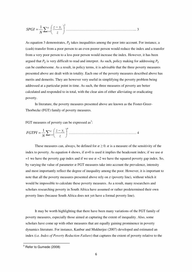
6
2
1
1∑
=
−=
q
i
i
z
yz
NSPGI …………………………………………………... 3
As equation 3 demonstrates, �� takes inequalities among the poor into account. For instance, a
(cash) transfer from a poor person to an even poorer person would reduce the index and a transfer
from a very poor person to a less poor person would increase the index. However, it has been
argued that �� is very difficult to read and interpret. As such, policy making for addressing ��
can be cumbersome. As a result, in policy terms, it is advisable that the three poverty measures
presented above are dealt with in totality. Each one of the poverty measures described above has
merits and demerits. They are however very useful in simplifying the poverty problem being
addressed at a particular point in time. As such, the three measures of poverty are better
calculated and responded to in total, with the clear aim of either alleviating or eradicating
poverty.
In literature, the poverty measures presented above are known as the Foster-Greer-
Thorbecke (FGT) family of poverty measures.
FGT measures of poverty can be expressed as3:
α
∑=
−=
q
i
i
z
yz
NFGTPI
1
1………………………………………………… 4
These measures can, always, be defined for � ≥ 0. � is a measure of the sensitivity of the
index to poverty. As equation 4 shows, if �=0 is used it implies the headcount index; if we use �
=1 we have the poverty gap index and if we use � =2 we have the squared poverty gap index. So,
by varying the value of parameter � FGT measures take into account the prevalence, intensity
and most importantly reflect the degree of inequality among the poor. However, it is important to
note that all the poverty measures presented above rely on � (poverty line), without which it
would be impossible to calculate these poverty measures. As a result, many researchers and
scholars researching poverty in South Africa have assumed or rather predetermined their own
poverty lines (because South Africa does not yet have a formal poverty line).
It may be worth highlighting that there have been many variations of the FGT family of
poverty measures, especially those aimed at capturing the extent of inequality. Also, some
scholars have come up with other measures that are equally gaining prominence in poverty
dynamics literature. For instance, Kanbur and Mukherjee (2007) developed and estimated an
index (i.e. Index of Poverty Reduction Failure) that captures the extent of poverty relative to the
3 Refer to Gumede (2008)
7
resources available in a particular society to eradicate poverty. Also, there is (Amartya) Sen
Poverty Index which captures dynamics in wellbeing of those below the poverty line.
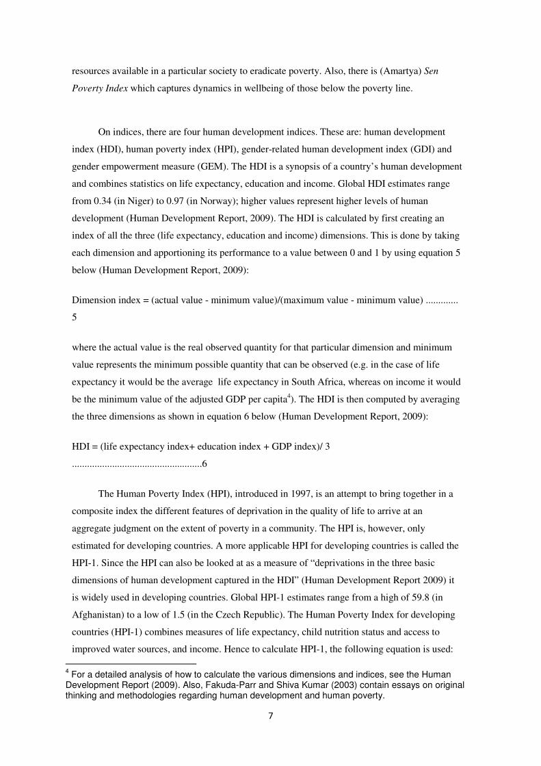
On indices, there are four human development indices. These are: human development
index (HDI), human poverty index (HPI), gender-related human development index (GDI) and
gender empowerment measure (GEM). The HDI is a synopsis of a country’s human development
and combines statistics on life expectancy, education and income. Global HDI estimates range
from 0.34 (in Niger) to 0.97 (in Norway); higher values represent higher levels of human
development (Human Development Report, 2009). The HDI is calculated by first creating an
index of all the three (life expectancy, education and income) dimensions. This is done by taking
each dimension and apportioning its performance to a value between 0 and 1 by using equation 5
below (Human Development Report, 2009):
Dimension index = (actual value - minimum value)/(maximum value - minimum value) .............
5
where the actual value is the real observed quantity for that particular dimension and minimum
value represents the minimum possible quantity that can be observed (e.g. in the case of life
expectancy it would be the average life expectancy in South Africa, whereas on income it would
be the minimum value of the adjusted GDP per capita4). The HDI is then computed by averaging
the three dimensions as shown in equation 6 below (Human Development Report, 2009):
HDI = (life expectancy index+ education index + GDP index)/ 3
....................................................6
The Human Poverty Index (HPI), introduced in 1997, is an attempt to bring together in a
composite index the different features of deprivation in the quality of life to arrive at an
aggregate judgment on the extent of poverty in a community. The HPI is, however, only
estimated for developing countries. A more applicable HPI for developing countries is called the
HPI-1. Since the HPI can also be looked at as a measure of “deprivations in the three basic
dimensions of human development captured in the HDI” (Human Development Report 2009) it
is widely used in developing countries. Global HPI-1 estimates range from a high of 59.8 (in
Afghanistan) to a low of 1.5 (in the Czech Republic). The Human Poverty Index for developing
countries (HPI-1) combines measures of life expectancy, child nutrition status and access to
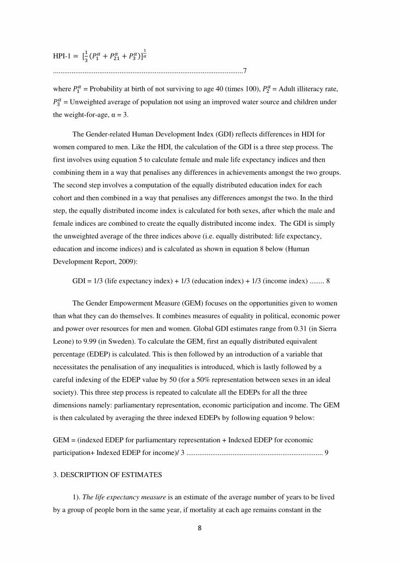
improved water sources, and income. Hence to calculate HPI-1, the following equation is used:
4 For a detailed analysis of how to calculate the various dimensions and indices, see the Human
Development Report (2009). Also, Fakuda-Parr and Shiva Kumar (2003) contain essays on original thinking and methodologies regarding human development and human poverty.
8
HPI-1 = [�
����
� + ���� + ��
��]�
�
.......................................................................................................7
where ��� = Probability at birth of not surviving to age 40 (times 100), ��
� = Adult illiteracy rate,
��� = Unweighted average of population not using an improved water source and children under
the weight-for-age, α = 3.
The Gender-related Human Development Index (GDI) reflects differences in HDI for
women compared to men. Like the HDI, the calculation of the GDI is a three step process. The
first involves using equation 5 to calculate female and male life expectancy indices and then
combining them in a way that penalises any differences in achievements amongst the two groups.
The second step involves a computation of the equally distributed education index for each
cohort and then combined in a way that penalises any differences amongst the two. In the third
step, the equally distributed income index is calculated for both sexes, after which the male and
female indices are combined to create the equally distributed income index. The GDI is simply
the unweighted average of the three indices above (i.e. equally distributed: life expectancy,
education and income indices) and is calculated as shown in equation 8 below (Human
Development Report, 2009):
GDI = 1/3 (life expectancy index) + 1/3 (education index) + 1/3 (income index) ........ 8
The Gender Empowerment Measure (GEM) focuses on the opportunities given to women
than what they can do themselves. It combines measures of equality in political, economic power
and power over resources for men and women. Global GDI estimates range from 0.31 (in Sierra
Leone) to 9.99 (in Sweden). To calculate the GEM, first an equally distributed equivalent
percentage (EDEP) is calculated. This is then followed by an introduction of a variable that
necessitates the penalisation of any inequalities is introduced, which is lastly followed by a
careful indexing of the EDEP value by 50 (for a 50% representation between sexes in an ideal
society). This three step process is repeated to calculate all the EDEPs for all the three
dimensions namely: parliamentary representation, economic participation and income. The GEM
is then calculated by averaging the three indexed EDEPs by following equation 9 below:
GEM = (indexed EDEP for parliamentary representation + Indexed EDEP for economic
participation+ Indexed EDEP for income)/ 3 .......................................................................... 9
3. DESCRIPTION OF ESTIMATES
1). The life expectancy measure is an estimate of the average number of years to be lived
by a group of people born in the same year, if mortality at each age remains constant in the

9
future. As a (crude) example, if 10% of a cohort dies before age 1 year, 40% dies between age 50
and 51 years, and 50% of the population dies between age 75 and 76 years, the life expectancy
for that cohort would be a simple weighted average of 57.6 years (or 10%*1+40%*50+50%*75).
Globally, life expectancy estimates in 2008 range from 32 years in Swaziland to 84 years in
Macau.
In this paper, life expectancy is reached by calculating the average change of dying at each
age, based on age specific mortality rates, and then aggregate these age specific mortality rates to
expected years of living. As an example, if 10% of all one year olds were reported to have died in
a particular year, the age specific mortality rate is 10%. If, in addition to that, 5% of all 2 year
olds and 5% of all 3 year olds died, there is 18.8% chance of dying by the age of 3 years. Based
on similar calculations for all age groups, average life expectancies are estimated.
NIDS collected information on the number of deaths in the household over the past 2 years
and the gender and age distribution of the deceased. The calculations here only include deaths
that occurred within one year of the survey time. There were a total of 913 deaths reported in the
NIDS data. In 136 of these cases, households reported that they did not know when the death had
taken place. In these cases, a 50% chance that the death had actually occurred within the last year
was ascribed. This, however risks the possibility of overestimating the mortality rates as
households are more likely to forget a date of a death that occurred 2 years earlier than one that
happened within the last year. Hence, it is plausible to assume that less than 50% of the death had
in actual fact occurred within the last year regardless of the fact that some might even have
occurred more than 2 years earlier, which would bring back issues of reliability of the mortality
rates. There is, however, no other better method available.
The estimated life expectancy rates and probabilities of living to age 3 years, 40 years and
60 years are reported in Table 1 below. The estimates suggest that South Africans live an average
life of 50 years. Women live, on average, 3 years longer than men and have average life
expectancies of 51 years compared to 48 years for men. This can be ascribed to the fact that
women live much healthier lifestyles than men. For example, women are less likely to engage in
life threatening habits (smoking, crime etc) than do men. Further, other causes of this might lie in
the role of the women in the average South African family. Women continue to be, by and large,
the bread winners in most families in South Africa. The data further suggests that males are also
almost twice as likely to die within the first year of their lives, than their female counterparts.
Blacks have the lowest life expectancy rate of all population groups. On average, Blacks
live for 45 years, while Coloureds live for 62 and 74 years, respectively. The estimate for Indians
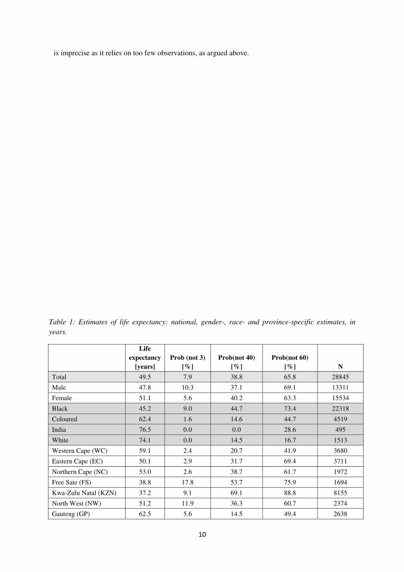
10
is imprecise as it relies on too few observations, as argued above.
Table 1: Estimates of life expectancy: national, gender-, race- and province-specific estimates, in
years.
Life
expectancy
[years]
Prob (not 3)
[%]
Prob(not 40)
[%]
Prob(not 60)
[%] N
Total 49.5 7.9 38.8 65.8 28845
Male 47.8 10.3 37.1 69.1 13311
Female 51.1 5.6 40.2 63.3 15534
Black 45.2 9.0 44.7 73.4 22318
Coloured 62.4 1.6 14.6 44.7 4519
India 76.5 0.0 0.0 28.6 495
White 74.1 0.0 14.5 16.7 1513
Western Cape (WC) 59.1 2.4 20.7 41.9 3680
Eastern Cape (EC) 50.1 2.9 31.7 69.4 3711
Northern Cape (NC) 53.0 2.6 38.7 61.7 1972
Free Sate (FS) 38.8 17.8 53.7 75.9 1694
Kwa-Zulu Natal (KZN) 37.2 9.1 69.1 88.8 8155
North West (NW) 51.2 11.9 36.3 60.7 2374
Gauteng (GP) 62.5 5.6 14.5 49.4 2638
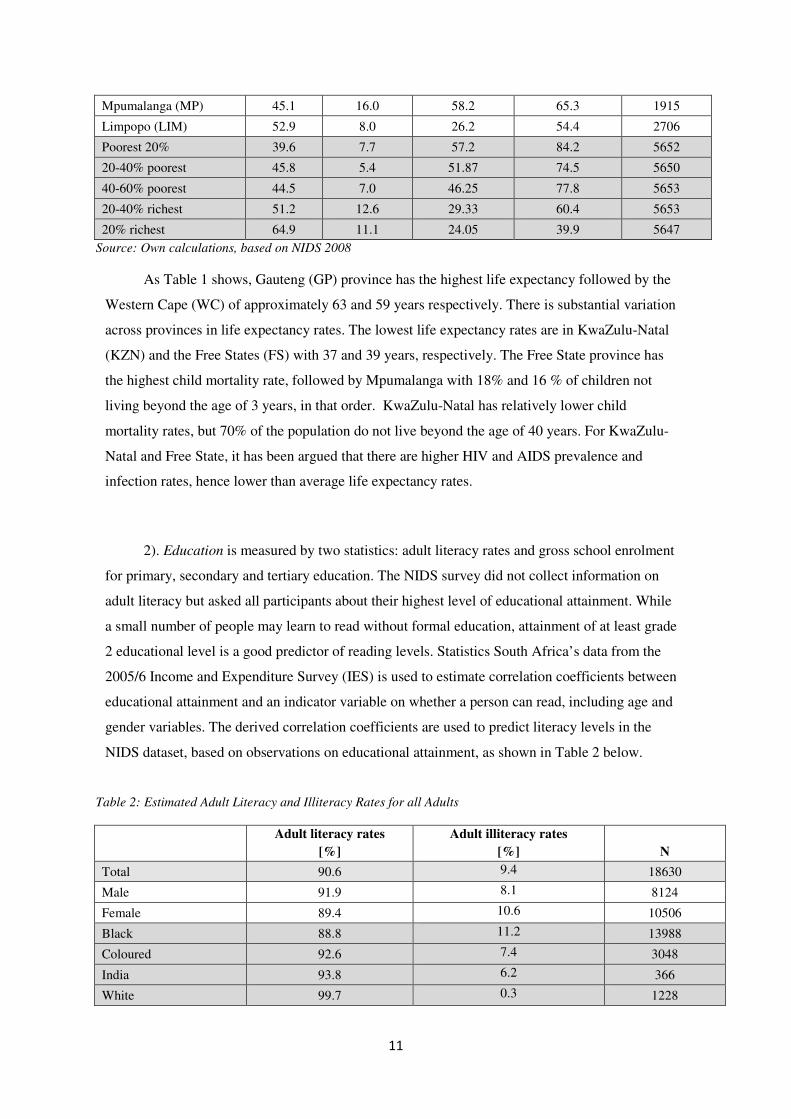
11
Mpumalanga (MP) 45.1 16.0 58.2 65.3 1915
Limpopo (LIM) 52.9 8.0 26.2 54.4 2706
Poorest 20% 39.6 7.7 57.2 84.2 5652
20-40% poorest 45.8 5.4 51.87 74.5 5650
40-60% poorest 44.5 7.0 46.25 77.8 5653
20-40% richest 51.2 12.6 29.33 60.4 5653
20% richest 64.9 11.1 24.05 39.9 5647
Source: Own calculations, based on NIDS 2008
As Table 1 shows, Gauteng (GP) province has the highest life expectancy followed by the
Western Cape (WC) of approximately 63 and 59 years respectively. There is substantial variation
across provinces in life expectancy rates. The lowest life expectancy rates are in KwaZulu-Natal
(KZN) and the Free States (FS) with 37 and 39 years, respectively. The Free State province has
the highest child mortality rate, followed by Mpumalanga with 18% and 16 % of children not
living beyond the age of 3 years, in that order. KwaZulu-Natal has relatively lower child
mortality rates, but 70% of the population do not live beyond the age of 40 years. For KwaZulu-
Natal and Free State, it has been argued that there are higher HIV and AIDS prevalence and
infection rates, hence lower than average life expectancy rates.
2). Education is measured by two statistics: adult literacy rates and gross school enrolment
for primary, secondary and tertiary education. The NIDS survey did not collect information on
adult literacy but asked all participants about their highest level of educational attainment. While
a small number of people may learn to read without formal education, attainment of at least grade
2 educational level is a good predictor of reading levels. Statistics South Africa’s data from the
2005/6 Income and Expenditure Survey (IES) is used to estimate correlation coefficients between
educational attainment and an indicator variable on whether a person can read, including age and
gender variables. The derived correlation coefficients are used to predict literacy levels in the
NIDS dataset, based on observations on educational attainment, as shown in Table 2 below.
Table 2: Estimated Adult Literacy and Illiteracy Rates for all Adults
Adult literacy rates
[%]
Adult illiteracy rates
[%] N
Total 90.6 9.4 18630
Male 91.9 8.1 8124
Female 89.4 10.6 10506
Black 88.8 11.2 13988
Coloured 92.6 7.4 3048
India 93.8 6.2 366
White 99.7 0.3 1228
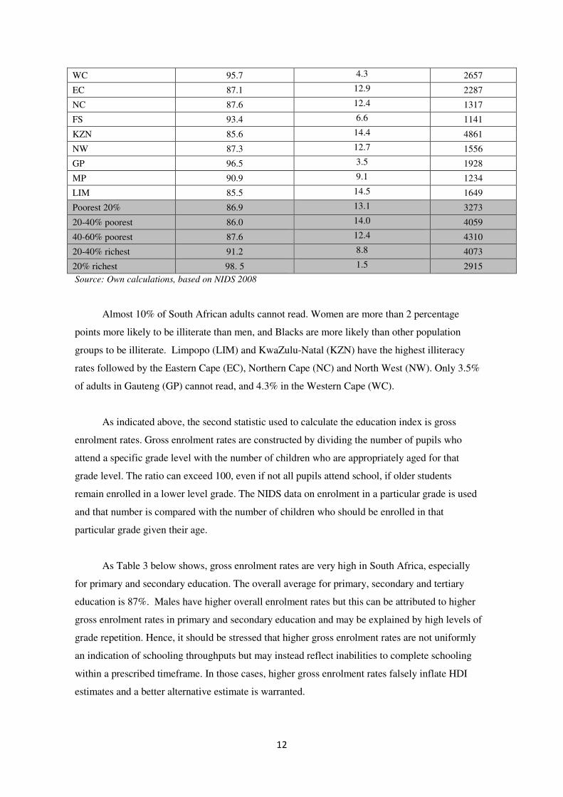
12
WC 95.7 4.3 2657
EC 87.1 12.9 2287
NC 87.6 12.4 1317
FS 93.4 6.6 1141
KZN 85.6 14.4 4861
NW 87.3 12.7 1556
GP 96.5 3.5 1928
MP 90.9 9.1 1234
LIM 85.5 14.5 1649
Poorest 20% 86.9 13.1 3273
20-40% poorest 86.0 14.0 4059
40-60% poorest 87.6 12.4 4310
20-40% richest 91.2 8.8 4073
20% richest 98. 5 1.5 2915
Source: Own calculations, based on NIDS 2008
Almost 10% of South African adults cannot read. Women are more than 2 percentage
points more likely to be illiterate than men, and Blacks are more likely than other population
groups to be illiterate. Limpopo (LIM) and KwaZulu-Natal (KZN) have the highest illiteracy
rates followed by the Eastern Cape (EC), Northern Cape (NC) and North West (NW). Only 3.5%
of adults in Gauteng (GP) cannot read, and 4.3% in the Western Cape (WC).
As indicated above, the second statistic used to calculate the education index is gross
enrolment rates. Gross enrolment rates are constructed by dividing the number of pupils who
attend a specific grade level with the number of children who are appropriately aged for that
grade level. The ratio can exceed 100, even if not all pupils attend school, if older students
remain enrolled in a lower level grade. The NIDS data on enrolment in a particular grade is used
and that number is compared with the number of children who should be enrolled in that
particular grade given their age.
As Table 3 below shows, gross enrolment rates are very high in South Africa, especially
for primary and secondary education. The overall average for primary, secondary and tertiary
education is 87%. Males have higher overall enrolment rates but this can be attributed to higher
gross enrolment rates in primary and secondary education and may be explained by high levels of
grade repetition. Hence, it should be stressed that higher gross enrolment rates are not uniformly
an indication of schooling throughputs but may instead reflect inabilities to complete schooling
within a prescribed timeframe. In those cases, higher gross enrolment rates falsely inflate HDI
estimates and a better alternative estimate is warranted.

13
Only 10% of females and 7% of males are enrolled in tertiary education. Coloureds have
higher gross enrolment rates in primary school and lower enrolment rates than other population
groups in secondary and tertiary levels. Geographically, the lowest gross enrolment rates are in
the Western Cape (WC) and the North West (NW). Again, this may be for two different reasons:
improved access to schooling in the WC and higher repetition rates in the NW. The North West
in the only province with less than 100% gross enrolment in primary education.
Table 3: Enrolment rates for different levels of education
Primary
education
enrolment rate
Secondary
education
enrolment rate
Tertiary education
enrolment rate
Total enrolment
rates
Total 125 113 9 87
Male 138 113 7 91
Female 113 115 10 83
Black 123 118 8 88
Coloured 132 79 5 79
India 115 106 19 82
White 100 101 18 72
WC 126 82 7 76
EC 126 98 5 85
NC 119 106 7 86
FS 115 109 12 84
KZN 127 109 6 88
NW 93 126 12 79
GP 143 127 15 91
MP 111 128 10 87
LIM 118 134 12 94
Poorest 20% 128 104 2 86
20-40% poorest 120 102 6 85
40-60% poorest 113 110 8 81
20-40% richest 111 123 11 80
20% richest 119 125 25 88

14
Source: Own calculations, based on NIDS 2008
3). Living standards are captured through the income measure using GDP per capita.
Based on Statistics South Africa national income and mid-year population estimates and World
Bank Purchasing Power Parity (PPP) conversion rates GDP per capita in 2008 was $10,109. This
level of income is adjusted to variations across gender, race and provinces using household
income averages. The results are presented in Table 4 below.
Table 4: Average household income per capita, GDP per capita in PPP US$, and share living in poverty
Income per capita
[Rand]
Converted to GDP per
capita
Share living below poverty
line [%]
Total 1722 10109 47
Male 1856 10897 46
Female 1597 9372 51
Black 935 5489 56
Coloured 1536 9016 27
India 3776 22164 9
White 7607 44657 2
WC 2325 13648 23
EC 869 5102 64
NC 1501 8811 33
FS 1599 9387 46
KZN 1360 7982 63
NW 1501 8808 43
GP 2688 15782 30
MP 2029 11908 44
LIM 1012 5942 64
Poorest 20% 143 842 100
20-40% poorest 313 1839 100
40-60% poorest 554 3255 38.9
20-40% richest 1209 7095 0
20% richest 6395 37538 0
Source: Own calculations, based on NIDS 2008
15
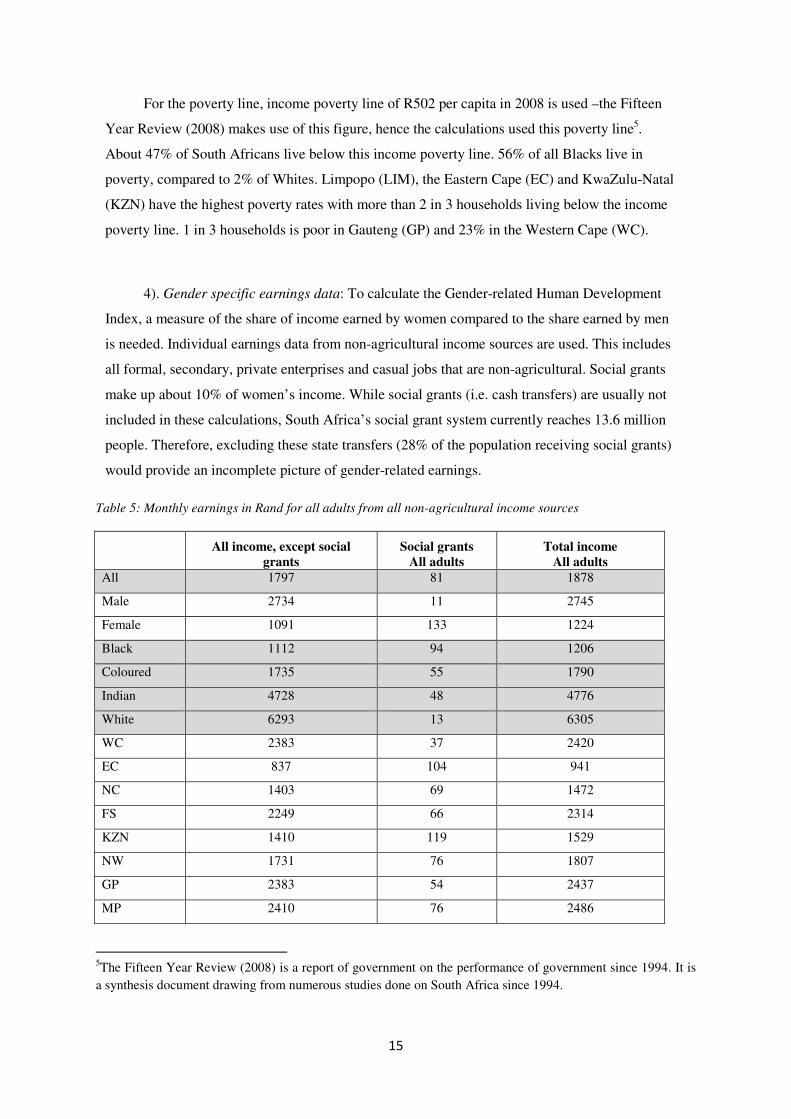
For the poverty line, income poverty line of R502 per capita in 2008 is used –the Fifteen
Year Review (2008) makes use of this figure, hence the calculations used this poverty line5.
About 47% of South Africans live below this income poverty line. 56% of all Blacks live in
poverty, compared to 2% of Whites. Limpopo (LIM), the Eastern Cape (EC) and KwaZulu-Natal
(KZN) have the highest poverty rates with more than 2 in 3 households living below the income
poverty line. 1 in 3 households is poor in Gauteng (GP) and 23% in the Western Cape (WC).
4). Gender specific earnings data: To calculate the Gender-related Human Development
Index, a measure of the share of income earned by women compared to the share earned by men
is needed. Individual earnings data from non-agricultural income sources are used. This includes
all formal, secondary, private enterprises and casual jobs that are non-agricultural. Social grants
make up about 10% of women’s income. While social grants (i.e. cash transfers) are usually not
included in these calculations, South Africa’s social grant system currently reaches 13.6 million
people. Therefore, excluding these state transfers (28% of the population receiving social grants)
would provide an incomplete picture of gender-related earnings.
Table 5: Monthly earnings in Rand for all adults from all non-agricultural income sources
All income, except social
grants
Social grants
All adults
Total income
All adults
All 1797 81 1878
Male 2734 11 2745
Female 1091 133 1224
Black 1112 94 1206
Coloured 1735 55 1790
Indian 4728 48 4776
White 6293 13 6305
WC 2383 37 2420
EC 837 104 941
NC 1403 69 1472
FS 2249 66 2314
KZN 1410 119 1529
NW 1731 76 1807
GP 2383 54 2437
MP 2410 76 2486
5The Fifteen Year Review (2008) is a report of government on the performance of government since 1994. It is
a synthesis document drawing from numerous studies done on South Africa since 1994.

16
LIM 1001 115 1116
Source: Own calculations, based on NIDS 2008
Men earn, on average, R2,745 per month or more than twice the average female non-
agricultural earnings. The black population earn R1,200 or less than a sixth of the average
monthly non-agricultural earnings of the white population group. The Eastern Cape (EC) and
Limpopo (LIM) have the lowest average non-agricultural earnings per month, while the Western
Cape (WC), Gauteng (GP) and Mpumalanga (MP) have the highest average monthly earnings.
These findings are consistent with those found by other researchers regarding labour market
participation and remuneration. On average, women are less likely to participate in the formal
labour market, fewer women than men are self-employed and women work fewer hours on
average than men and are more likely to be in casual and less well paid jobs.
5). Safe, clean water: Data on lack of access to improved sources of water is collected
directly in the NIDS. Missing values are imputed based on geographical areas, household income
and type of dwelling. As Table 6 below indicates, about 7% of all South Africans rely on springs,
streams, pools or dams for household water. Blacks are the only population group to lack access
to improved water sources. The backlog is severe in the Eastern Cape (EC) where 23% of South
Africans live without improved water and KwaZulu-Natal (14%).
5). Underweight children below age 5 years: NIDS fieldworkers measured weight and
heights for all children under the age of 15 years. That information is used to construct a Body
Mass Index (BMI) measure and categorize children who are underweight using international age
specific standards. As Table 6 below shows, underweight in children below the age of 5 years is
a particular problem for Coloureds (14%). Black and White children are less at risk with 8% and
7% measured to be underweight. Girls are more than twice as likely to be underweight than boys.
Northern Cape (NC) and Mpumalanga (MP) have the highest rate of underweight children, while
KwaZulu-Natal (KZN) has the lowest rate, at just 5%.

17
Table 6: Access to safe improved water and child nutritional status
Share of population who lack
access to clean drinking water
[%]
Share of under-5 who are
underweight [%]
Total 6.7 8.2
Male 6.3 4.7
Female 7.1 11.5
Black 8.4 7.7
Coloured 0.7 13.5
India 0.0 10.0
White 0.0 6.7
WC 0.2 8.8
EC 23.1 9.4
NC 0.2 12.6
FS 0.0 6.8
KZN 13.7 4.9
NW 0.3 9.4
GP 0.0 9.0
MP 0.4 12.5
LIM 6.0 8.5
Poorest 20% 14.0 9.3
20-40% poorest 11.9 9.1
40-60% poorest 4.4 7.1
20-40% richest 2.3 8.3
20% richest 0.9 5.2
4. INDICES: HUMAN DEVELOPMENT AND HUMAN POVERTY
The aggregate national HDI for 2008 is 0.69 – incidentally the same figure for the Gini
Coefficient. There is no substantial difference in the HDI for women and men separately. Blacks
have the lowest HDI at 0.63, compared to that of Whites at 0.91. As such, the black population
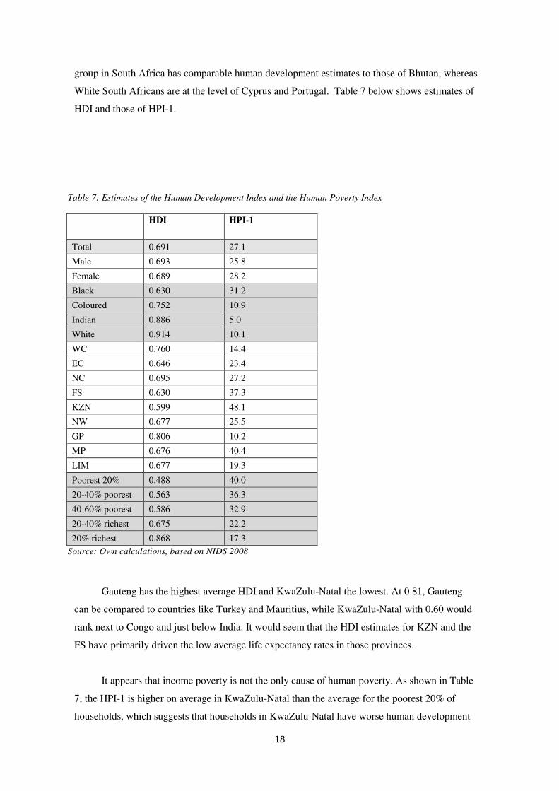
18
group in South Africa has comparable human development estimates to those of Bhutan, whereas
White South Africans are at the level of Cyprus and Portugal. Table 7 below shows estimates of
HDI and those of HPI-1.
Table 7: Estimates of the Human Development Index and the Human Poverty Index
HDI
HPI-1
Total 0.691 27.1
Male 0.693 25.8
Female 0.689 28.2
Black 0.630 31.2
Coloured 0.752 10.9
Indian 0.886 5.0
White 0.914 10.1
WC 0.760 14.4
EC 0.646 23.4
NC 0.695 27.2
FS 0.630 37.3
KZN 0.599 48.1
NW 0.677 25.5
GP 0.806 10.2
MP 0.676 40.4
LIM 0.677 19.3
Poorest 20% 0.488 40.0
20-40% poorest 0.563 36.3
40-60% poorest 0.586 32.9
20-40% richest 0.675 22.2
20% richest 0.868 17.3
Source: Own calculations, based on NIDS 2008
Gauteng has the highest average HDI and KwaZulu-Natal the lowest. At 0.81, Gauteng
can be compared to countries like Turkey and Mauritius, while KwaZulu-Natal with 0.60 would
rank next to Congo and just below India. It would seem that the HDI estimates for KZN and the
FS have primarily driven the low average life expectancy rates in those provinces.
It appears that income poverty is not the only cause of human poverty. As shown in Table
7, the HPI-1 is higher on average in KwaZulu-Natal than the average for the poorest 20% of
households, which suggests that households in KwaZulu-Natal have worse human development

19
on average than can be attributed to their income status. Whites and Indians also have better
human development indices than the average for the richest 20% of all South Africans, which
suggests that there are additional factors than household income that determine inter-racial
differences in human development and is captured in much lower life expectancy rates for non-
white population groups. It is in this context that an argument is made that the legacy of
apartheid remains profound and/or that government has not succeeded in racial redress.
The other index calculated is the Gender-related Human Development Index. It is a
measure of the human development of women in relation to that of men. It is at 99.84, one of the
highest in the world and suggests that South Africa has fairly equal levels of human development
for women and men. This however ignores stark differences in some sub-components such as
income (where men fare much better) and life expectancy (where women do better).
5. WHAT IS TO BE DONE?
As agued by some, the catalyst to (structural) poverty and inequality is employment along
with the further improvement of human capital. In this context, it is perhaps understandable that
poverty and inequality remains this high in South Africa. Many proposals have been made on
how to create more jobs in SA (see Natrass and Seekings 2006, as an example). The recent
proposals include a wage subsidy, along other active labour market interventions. The wage
subsidy, if conceptualized and implemented in a sound manner, is one of the possible solutions.
There is a set of ‘general’ interventions that any country that is serious about expanding
human capabilities should pursue: the set includes broadening economic participation, growing
the economy and ensuring that benefits of economic growth are shared equitably, ensuring access
to basic services, protecting the most vulnerable, and so on and so forth. Examining SA’s state of
human development and socio-economic transformation, a question remains as to whether the
country is making sufficient inroads to the successful implementation of the set of ‘general’
interventions. Given this, an argument can be made that SA should be better applying the
‘general’ interventions such as those highlighted here.
Besides issues related to the labour market and the set of ‘general’ interventions, it is hard
to think of other interventions that SA should pursue to further address poverty and inequality. In
particular, SA’s social protection mechanisms appear to be at the scale and level of other
comparable countries – such as Brazil, India, Mexico and possibly China – which appear to have
reduced poverty and inequality better than SA.
20
It could be that the fundamental challenge with SA is the economy – and this is the
complex challenge to address. It implies that there should be careful rethinking around
redistributive policies. The further restructuring of the economy in order that it benefits every
South African could be the answer. The compounding challenge is that there are trade-offs that
have to be made. In addition, as argued by some, there may be different sets of policy
interventions for poverty on one hand and for inequality on the other hand. Lastly, historically or
at least in economic theory, speedier economic growth may in the short to medium term worsen
inequality.
6. CONCLUDING REMARKS
In summary, the South African HDI for 2008 equates Botswana’s 2007 HDI and would
have ranked South Africa in place 125 rather than South Africa’s 2007 ranking of 129. At 0.63,
the black population group in South Africa has comparable human development estimates to
those of Bhutan, while those of white South Africans are at the level of Cyprus and Portugal.
Gauteng has the highest average HDI and KwaZulu-Natal the lowest. On average, the poorest
20% of South African households have similar human development as in Zambia and Malawi,
while the richest 20% of households on average are at the same level of human development as
Argentina and Latvia. Inequalities in human development across population groups in South
Africa are larger than between the rich and the poor – this mirrors a very high Gini Coefficient.
The rich non-white population groups have benefitted from improved income but that has not
translated into higher life expectancy and longevity, as an example. Regarding (human) poverty
and economic inequality, the numbers are still very high.
In terms of policy matters, Habib and Bentley (2008) provide pointers on the main
challenge confronting SA: that racial redress has not gone far enough. The same can be said
regarding gender redress and spatial redress, hence the skewed income distribution and relatively
high human poverty. It would seem that the issue is fundamentally with the economy. The other
policy issues requiring attention pertain to redistributive policies – the policies themselves and
their implementation. In the short-term to medium term, something could be done about the
labour market in order that it can absorb more entrants along further improvements in human
capital.
21
SELECTED REFERENCES
Argent, J (2009). Household Income: Report on NIDS Wave 1 – Technical Report No. 3, SALDRU,
Cape Town
Bhorat, H & Van der Westhuizen, C (2010). Poverty, Inequality and the Nature of Economic Growth
in South Africa. In: Misra-Dexter, N & February, J. Testing Democracy: Which way is South Africa
going? IDASA: Cape Town
Fakuda-Parr, S and Shiva Kumar, AK (eds) (2003). Readings in Human Development, Oxford:
Oxford University Press
Gumede, V (2008). Poverty and Second Economy Dynamics in South Africa: An attempt to measure
the extent of the problem and clarify concepts. Development Policy Research Unit Working Paper
08/133. University of Cape Town, Cape Town
Gumede, V (2009). Attempts to include the excluded: Anti-poverty Strategy for South Africa, In:
2009 Transformation Audit, Institute of Justice and Reconciliation, IJR: Cape Town
Habib, A and Bentley, K (2008). Racial Redress and Citizenship in South Africa. Cape Town: HSRC
Press
Kanbur, R and Mukherjee, D (2007). Poverty, Relative to the Ability to Eradicate it: An Index
of Poverty Reduction Failure. Department of Applied Economics and Management, Cornell
University, Working Paper 02
Moultrie, T (2009). Questions on Demography for the NIDS, Background Paper, SALDRU,
University of Cape Town, Cape Town
Nattrass, N and Seekings, J (2006). Class, Race, and Inequality in South Africa. Durban: UKZN Press
Policy Coordination and Advisory Services (2008). Towards Fifteen Year Review. The Presidency:
Pretoria
United Nations Development Programme (2009). Human Development Report 2009. Palgrave
Macmillan, New York.