inequality, costly redistribution and welfare in an...
TRANSCRIPT

A Motivating ExampleEconomic Model
Calibration and Counterfactuals
Inequality, Costly Redistribution and Welfare inan Open Economy
Pol AntrasHarvard University
Alonso de GortariHarvard University
Oleg ItskhokiPrinceton University
ITSG - December 10, 2015
Antras, de Gortari and Itskhoki Inequality, Costly Redistribution and Welfare in an Open Economy 1 / 39

A Motivating ExampleEconomic Model
Calibration and Counterfactuals
Introduction
I Trade integration raises real income but often increases inequalityand might make some worse off
I Standard approach to demonstrating and quantifying the gains fromtrade largely ignores trade-induced inequality
I Kaldor-Hicks compensation principle
I Two basic shortcomings with this approach:
I How much compensation/redistribution actually takes place?
I Is this redistribution costless, as the Kaldor-Hicks approach assumes?
I These issues are relevant not just for trade, but also for any policywith redistributive effects
Antras, de Gortari and Itskhoki Inequality, Costly Redistribution and Welfare in an Open Economy 2 / 39
A Motivating ExampleEconomic Model
Calibration and Counterfactuals
A Motivating Quote
“If, as will often happen, the best methods of compensation feasibleinvolve some loss in productive efficiency, this loss will have to be takeninto account.”
Hicks (1939, p. 712)
Antras, de Gortari and Itskhoki Inequality, Costly Redistribution and Welfare in an Open Economy 3 / 39

A Motivating ExampleEconomic Model
Calibration and Counterfactuals
This Paper
I We study welfare implications of trade liberalization in a model inwhich trade affects income distribution...
I ... and in which redistribution policies are constrained by informationfrictions (Mirrlees, 1971)
I Despite the fact that the tax system is progressive, trade increasesinequality in the after-tax distribution of income
I We propose two types of adjustments to standard welfare measures:
1. A ‘welfarist’ correction reflecting the preferences of aninequality-averse social planner
2. A ‘costly-redistribution’ correction capturing behavioral responses totrade-induced shifts across marginal tax rates
Antras, de Gortari and Itskhoki Inequality, Costly Redistribution and Welfare in an Open Economy 4 / 39

A Motivating ExampleEconomic Model
Calibration and Counterfactuals
Building Blocks
I Skeleton of Trade Model: Itskhoki (2008)
I Melitz (2003) with heterogeneous workers/entrepeneurs and a laborsupply decision
I Costly Redistribution: Nonlinear progressive tax system
I After-tax income is log-linear function of pre-tax income (great fit)
I Welfarist correction: constant degree of inequality- (or risk-) aversion
I widely used in Public Finance (veil of ignorance rationale)
I Model calibrated to fit 2007 U.S. data:
I distribution of skills calibrated to match U.S. distribution of(adjusted gross) income from IRS public records
I trade costs calibrated to match U.S. trade share
Antras, de Gortari and Itskhoki Inequality, Costly Redistribution and Welfare in an Open Economy 5 / 39

A Motivating ExampleEconomic Model
Calibration and Counterfactuals
0.46
0.48
0.50
0.52
0.54
0.56
0.58
0.60
7%
8%
9%
10%
11%
12%
13%
14%
1979 1981 1983 1985 1987 1989 1991 1993 1995 1997 1999 2001 2003 2005 2007
Openness and Inequality in the United States (1979‐2007)
Trade Share Gini of Market Income
Antras, de Gortari and Itskhoki Inequality, Costly Redistribution and Welfare in an Open Economy 6 / 39

A Motivating ExampleEconomic Model
Calibration and Counterfactuals
Related Literature
I Trade models with heterogeneous workers: Itskhoki (2008) but also
I matching/sorting models (see Grossman, and Costinot and Vogel forsurveys)
I models with imperfect labor markets (Helpman, Itskhoki, Redding...,and earlier Davidson and Matusz)
I Gains from trade and costly redistribution: Dixit and Norman(1986), Rodrik (1992), Spector (2001), Naito (2006)
I Old literature on Kaldor-Hicks: Kaldor (1939), Hicks (1939),Scitovszky (1941)
I Welfarist approach: Bergson (1938), Samuelson (1947), Diamond &Mirlees (1971), Saez more recently
I Costly-redistribution: Kaplow (2008), Hendren (2014)
Antras, de Gortari and Itskhoki Inequality, Costly Redistribution and Welfare in an Open Economy 7 / 39

A Motivating ExampleEconomic Model
Calibration and Counterfactuals
Road Map
1. A Motivating Example
2. Economic Model
3. Calibration
4. Counterfactuals: Inequality and the Gains from Trade
Antras, de Gortari and Itskhoki Inequality, Costly Redistribution and Welfare in an Open Economy 8 / 39

A Motivating ExampleEconomic Model
Calibration and Counterfactuals
Kaldor-Hicks PrincipleWelfarist CorrectionCostly Redistribution Correction
A Motivating Example
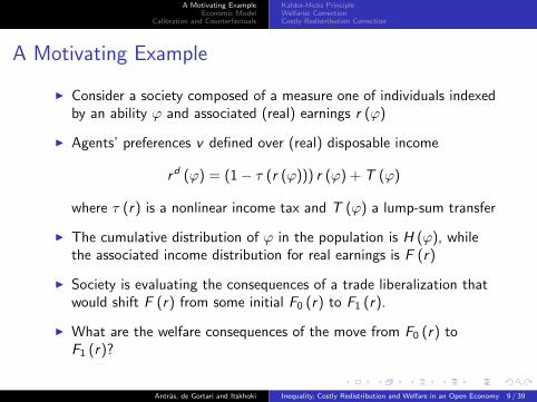
I Consider a society composed of a measure one of individuals indexedby an ability ϕ and associated (real) earnings r (ϕ)
I Agents’ preferences v defined over (real) disposable income
rd (ϕ) = (1− τ (r (ϕ))) r (ϕ) + T (ϕ)
where τ (r) is a nonlinear income tax and T (ϕ) a lump-sum transfer
I The cumulative distribution of ϕ in the population is H (ϕ), whilethe associated income distribution for real earnings is F (r)
I Society is evaluating the consequences of a trade liberalization thatwould shift F (r) from some initial F0 (r) to F1 (r).
I What are the welfare consequences of the move from F0 (r) toF1 (r)?
Antras, de Gortari and Itskhoki Inequality, Costly Redistribution and Welfare in an Open Economy 9 / 39

A Motivating ExampleEconomic Model
Calibration and Counterfactuals
Kaldor-Hicks PrincipleWelfarist CorrectionCostly Redistribution Correction
A Motivating Example
I Consider a society composed of a measure one of individuals indexedby an ability ϕ and associated (real) earnings r (ϕ)
I Agents’ preferences v defined over (real) disposable income
rd (ϕ) = (1− τ (r (ϕ))) r (ϕ) + T (ϕ)
where τ (r) is a nonlinear income tax and T (ϕ) a lump-sum transfer
I The cumulative distribution of ϕ in the population is H (ϕ), whilethe associated income distribution for real earnings is F (r)
I Society is evaluating the consequences of a trade liberalization thatwould shift F (r) from some initial F0 (r) to F1 (r).
I What are the welfare consequences of the move from F0 (r) toF1 (r)?
Antras, de Gortari and Itskhoki Inequality, Costly Redistribution and Welfare in an Open Economy 9 / 39

A Motivating ExampleEconomic Model
Calibration and Counterfactuals
Kaldor-Hicks PrincipleWelfarist CorrectionCostly Redistribution Correction
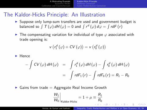
The Kaldor-Hicks Principle: An IllustrationI Suppose only lump-sum transfers are used and government budget is
balanced so∫T (ϕ) dH (ϕ) = 0 and
∫rd (ϕ) dϕ =
∫rdF (r)
I The compensating variation for individual of type ϕ associated withtrade opening is:
v(rd1 (ϕ) + CV (ϕ)
)= v
(rd0 (ϕ)
)
I Hence
−∫
CV (ϕ) dH (ϕ) =
∫rd1 (ϕ) dH (ϕ)−
∫rd0 (ϕ) dH (ϕ)
=
∫rdF1 (r)−
∫rdF0 (r) = R1 − R0
I Gains from trade = Aggregate Real Income Growth
W1
W0
∣∣∣∣Kaldor-Hicks
= 1 + µ ≡ R1
R0
Antras, de Gortari and Itskhoki Inequality, Costly Redistribution and Welfare in an Open Economy 10 / 39

A Motivating ExampleEconomic Model
Calibration and Counterfactuals
Kaldor-Hicks PrincipleWelfarist CorrectionCostly Redistribution Correction
The Kaldor-Hicks Principle: An IllustrationI Suppose only lump-sum transfers are used and government budget is
balanced so∫T (ϕ) dH (ϕ) = 0 and
∫rd (ϕ) dϕ =
∫rdF (r)
I The compensating variation for individual of type ϕ associated withtrade opening is:
v(rd1 (ϕ) + CV (ϕ)
)= v
(rd0 (ϕ)
)I Hence
−∫
CV (ϕ) dH (ϕ) =
∫rd1 (ϕ) dH (ϕ)−
∫rd0 (ϕ) dH (ϕ)
=
∫rdF1 (r)−
∫rdF0 (r) = R1 − R0
I Gains from trade = Aggregate Real Income Growth
W1
W0
∣∣∣∣Kaldor-Hicks
= 1 + µ ≡ R1
R0
Antras, de Gortari and Itskhoki Inequality, Costly Redistribution and Welfare in an Open Economy 10 / 39
A Motivating ExampleEconomic Model
Calibration and Counterfactuals
Kaldor-Hicks PrincipleWelfarist CorrectionCostly Redistribution Correction
Pros and Cons of the Kaldor-Hicks Principle
I Principle does not rely on interpersonal comparisons of utility
I indirect utility can be heterogeneous across agentsI result relies on ordinal rather than cardinal preferencesI notion of efficiency argued to be free of value judgments
I What if redistribution does not take place and the losers are notcompensated?
I under the veil of ignorance, agents see a probability distribution overpotential outcomes (need cardinal preferences)
I risk aversion ≈ inequality aversion
I Even if some redistribution takes place, whenever it is costly,shouldn’t W1/W0 reflect those costs?
I Dixit and Norman (1986) showed that W1/W0 > 1 using a coarse setof tax policies - but how large is W1/W0?
Antras, de Gortari and Itskhoki Inequality, Costly Redistribution and Welfare in an Open Economy 11 / 39

A Motivating ExampleEconomic Model
Calibration and Counterfactuals
Kaldor-Hicks PrincipleWelfarist CorrectionCostly Redistribution Correction
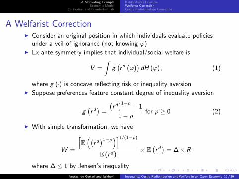
A Welfarist CorrectionI Consider an original position in which individuals evaluate policies
under a veil of ignorance (not knowing ϕ)I Ex-ante symmetry implies that individual/social welfare is
V =
∫g(rd (ϕ)
)dH (ϕ) , (1)
where g (·) is concave reflecting risk or inequality aversion
I Suppose preferences feature constant degree of inequality aversion
g(rd)
=
(rd)1−ρ − 1
1− ρfor ρ ≥ 0 (2)
I With simple transformation, we have
W =
[E((
rd)1−ρ
)]1/(1−ρ)
E (rd)× E
(rd)
= ∆× R
where ∆ ≤ 1 by Jensen’s inequality
Antras, de Gortari and Itskhoki Inequality, Costly Redistribution and Welfare in an Open Economy 12 / 39

A Motivating ExampleEconomic Model
Calibration and Counterfactuals
Kaldor-Hicks PrincipleWelfarist CorrectionCostly Redistribution Correction
A Welfarist CorrectionI Consider an original position in which individuals evaluate policies
under a veil of ignorance (not knowing ϕ)I Ex-ante symmetry implies that individual/social welfare is
V =
∫g(rd (ϕ)
)dH (ϕ) , (1)
where g (·) is concave reflecting risk or inequality aversionI Suppose preferences feature constant degree of inequality aversion
g(rd)
=
(rd)1−ρ − 1
1− ρfor ρ ≥ 0 (2)
I With simple transformation, we have
W =
[E((
rd)1−ρ
)]1/(1−ρ)
E (rd)× E
(rd)
= ∆× R
where ∆ ≤ 1 by Jensen’s inequality
Antras, de Gortari and Itskhoki Inequality, Costly Redistribution and Welfare in an Open Economy 12 / 39

A Motivating ExampleEconomic Model
Calibration and Counterfactuals
Kaldor-Hicks PrincipleWelfarist CorrectionCostly Redistribution Correction
Welfarist Correction: Two Special Cases
I Suppose H (ϕ) is such that the distribution of disposable income is
Pareto: ∆ =(
1+G1−G(1−2ρ)
)1/(1−ρ)1−G1+G
Lognormal: ∆ = exp{−ρ[Φ−1
(1+G
2
)]2}where G is the Gini coefficient of the distribution of rd
I W increases in mean income R but decreases in inequality G
I Notice that in both cases
W1
W0
∣∣∣∣Welfarist
=∆ (G1; ρ)
∆ (G0; ρ)× (1 + µ) , (3)
Antras, de Gortari and Itskhoki Inequality, Costly Redistribution and Welfare in an Open Economy 13 / 39

A Motivating ExampleEconomic Model
Calibration and Counterfactuals
Kaldor-Hicks PrincipleWelfarist CorrectionCostly Redistribution Correction
A Costly Redistribution CorrectionI Suppose now that lump-sum transfers are not feasible and
redistribution has to have through the income tax-transfer system
I Focus on the particular case (as in Heathcoate et al., 2014) in which
1− τ (r) = k (r)−φ , (4)
for some constant k which can be set to ensure that the governmentbudget is balanced
I Average net-of-tax rates decrease in reported income at a constantrate φ, which captures the degree of progressivity of the tax system
I Behavioral response to taxation: positive, constant elasticity ofreported income to the net-of-marginal-tax rate:
ε ≡ ∂r
∂ (1− τm (r))
1− τm (r)
r> 0 (5)
Antras, de Gortari and Itskhoki Inequality, Costly Redistribution and Welfare in an Open Economy 14 / 39

A Motivating ExampleEconomic Model
Calibration and Counterfactuals
Kaldor-Hicks PrincipleWelfarist CorrectionCostly Redistribution Correction
A Costly Redistribution CorrectionI In such a case, we find that aggregate income can be written as
R = (1− φ)ε(Er)1+ε
(Er1−φ)ε · E (r1+εφ)
× E (r) = Θ× R
where R is potential revenue (in the absence of distortionary taxes)
I By Holder’s inequality, Θ ≤ 1
I Θ is reduced by mean preserving multiplicative spreads of the incomedistribution (increased inequality)
I Two parametric examples
Pareto: Θ = (1− φ)ε (1−φ)(1+G)−(1+εφ)2G(1−φ)(1+G)−2G
((1−φ)(1−G)
(1−φ)(1+G)−2G
)εLognormal: Θ = (1− φ)ε exp
{−φ
2ε(ε+1)
(1−φ)2
[Φ−1
(1+G
2
)]2}where G is the Gini of the distribution of disposable income
Antras, de Gortari and Itskhoki Inequality, Costly Redistribution and Welfare in an Open Economy 15 / 39

A Motivating ExampleEconomic Model
Calibration and Counterfactuals
Closed EconomyOpen EconomyTrade and Inequality
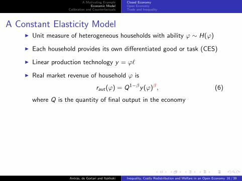
A Constant Elasticity ModelI Unit measure of heterogeneous households with ability ϕ ∼ H(ϕ)
I Each household provides its own differentiated good or task (CES)
I Linear production technology y = ϕ`
I Real market revenue of household ϕ is
raut(ϕ) = Q1−βy(ϕ)β , (6)
where Q is the quantity of final output in the economy
I Households have utility over consumption and labor:
u(ϕ) = c(ϕ)− 1
γ`(ϕ)γ , γ > 1 (7)
I Consumption equals after-tax income:
r(ϕ)− T(r(ϕ)
)= kr(ϕ)1−φ, (8)
and government runs balanced budget
Antras, de Gortari and Itskhoki Inequality, Costly Redistribution and Welfare in an Open Economy 16 / 39
A Motivating ExampleEconomic Model
Calibration and Counterfactuals
Closed EconomyOpen EconomyTrade and Inequality
A Constant Elasticity ModelI Unit measure of heterogeneous households with ability ϕ ∼ H(ϕ)
I Each household provides its own differentiated good or task (CES)
I Linear production technology y = ϕ`
I Real market revenue of household ϕ is
raut(ϕ) = Q1−βy(ϕ)β , (6)
where Q is the quantity of final output in the economy
I Households have utility over consumption and labor:
u(ϕ) = c(ϕ)− 1
γ`(ϕ)γ , γ > 1 (7)
I Consumption equals after-tax income:
r(ϕ)− T(r(ϕ)
)= kr(ϕ)1−φ, (8)
and government runs balanced budget
Antras, de Gortari and Itskhoki Inequality, Costly Redistribution and Welfare in an Open Economy 16 / 39
A Motivating ExampleEconomic Model
Calibration and Counterfactuals
Closed EconomyOpen EconomyTrade and Inequality
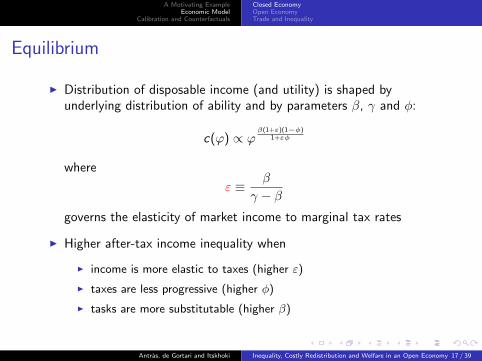
Equilibrium
I Distribution of disposable income (and utility) is shaped byunderlying distribution of ability and by parameters β, γ and φ:
c(ϕ) ∝ ϕβ(1+ε)(1−φ)
1+εφ
where
ε ≡ β
γ − βgoverns the elasticity of market income to marginal tax rates
I Higher after-tax income inequality when
I income is more elastic to taxes (higher ε)
I taxes are less progressive (higher φ)
I tasks are more substitutable (higher β)
Antras, de Gortari and Itskhoki Inequality, Costly Redistribution and Welfare in an Open Economy 17 / 39

A Motivating ExampleEconomic Model
Calibration and Counterfactuals
Closed EconomyOpen EconomyTrade and Inequality
Social Welfare
I With a constant degree of inequality aversion ρ, we can write
W = ∆× Θ× W
where
∆ =
[E((
rd)1−ρ
)]1/(1−ρ)
E (rd)
Θ = (1 + εφ) (1− φ)εκ[
(Er)1+ε
(Er1−φ)ε · E (r1+εφ)
]κand κ = 1/ (1− (1− β)(1 + ε)) > 1.
I ∆ is the same welfarist correction as in our example
I Θ is a slightly modified costly-redistribution correction
I W is welfare in a hypothetical ‘Kaldor-Hicks’ economy
Antras, de Gortari and Itskhoki Inequality, Costly Redistribution and Welfare in an Open Economy 18 / 39

A Motivating ExampleEconomic Model
Calibration and Counterfactuals
Closed EconomyOpen EconomyTrade and Inequality
A First Look at the Data
1980 1985 1990 1995 2000 20050.8
0.9
1
1.1
1.2
1.3
1.4
1.5Real Adjusted Gross Income in the United States (1979-2007)
Mean IncomeMedian Income10th Percentile
Antras, de Gortari and Itskhoki Inequality, Costly Redistribution and Welfare in an Open Economy 19 / 39

A Motivating ExampleEconomic Model
Calibration and Counterfactuals
Closed EconomyOpen EconomyTrade and Inequality
Calibration: U.S. Income Growth (1979-2007)
I Use U.S. Individual Income Tax Public Use Sample to calibratedistribution of market income
I approximately 3.5 million anonymized tax returns
I use NBER weights to ensure this is a representative sample
I we map market income to adjusted gross income in line 37 of IRSForm 1040
I Use CBO data on before-tax and after-tax/transfer income tocalibrate the degree of tax progressivity φ
I Elasticity of substitution = 4 (β = 3/4)
I BEJK (2003), Broda and Weinstein (2006)
I Experiment with various values of ε and ρ
I Benchmark ε = 0.5 and ρ = 1
Antras, de Gortari and Itskhoki Inequality, Costly Redistribution and Welfare in an Open Economy 20 / 39

A Motivating ExampleEconomic Model
Calibration and Counterfactuals
Closed EconomyOpen EconomyTrade and Inequality
Calibrating the Income DistributionI Lognormal provides a reasonably good approximation, but it does a
poor fit for the right-tail of the distribution, which looks Pareto
r6 8 10 12
0
0.1
0.2
0.3
0.4
0.5
0.6
0.7
0.8
0.9
1Income Distribution CDF
Data (Non-Parametric Fit)Lognormal Fit
r #1050 1 2 3 4 5
1
1.5
2
2.5Empirical Pareto Coefficient
Antras, de Gortari and Itskhoki Inequality, Costly Redistribution and Welfare in an Open Economy 21 / 39

A Motivating ExampleEconomic Model
Calibration and Counterfactuals
Closed EconomyOpen EconomyTrade and Inequality
Calibrating Tax ProgressivityI Equation (4) may seem ad hoc, but it fits U.S. data remarkably well
(similar fit with PSID data)
y = 0.818x + 2.002 R² = 0.988
9
10
11
12
13
14
9 10 11 12 13 14
Log
Inco
me
Afte
r Tax
es a
nd T
rans
fers
Log Market Income
Antras, de Gortari and Itskhoki Inequality, Costly Redistribution and Welfare in an Open Economy 22 / 39

A Motivating ExampleEconomic Model
Calibration and Counterfactuals
Closed EconomyOpen EconomyTrade and Inequality
U.S. Progressivity Over Time
0.1
.2.3
.4
1979 1983 1987 1991 1995 1999 2003 2007Year
Degree of Progressivity
Antras, de Gortari and Itskhoki Inequality, Costly Redistribution and Welfare in an Open Economy 23 / 39

A Motivating ExampleEconomic Model
Calibration and Counterfactuals
Closed EconomyOpen EconomyTrade and Inequality
Evolution of ∆ and Θ Over Time
": Inequality Aversion0.55 0.6 0.65 0.7 0.75 0.8
(1+0?
)#5: C
ostly
Red
istri
butio
n
0.85
0.86
0.87
0.88
0.89
0.9
0.91
0.92
0.93(",(1+0? )# 5 ) Phase Diagram, ;=1, 0=0.5
Antras, de Gortari and Itskhoki Inequality, Costly Redistribution and Welfare in an Open Economy 24 / 39

A Motivating ExampleEconomic Model
Calibration and Counterfactuals
Closed EconomyOpen EconomyTrade and Inequality
Social Welfare and Counterfactuals
I Mean real income grew 44.2% over 1979-2007, or 1.32% per year.
I For the logarithmic case (ρ = 1), the implied annual growth rate insocial welfare is down to 0.34%.
I partly due to observed decline in progressivity
I By how much would real income and social welfare have increased ifφ had been held constant at its 1979 level? For ρ = 1 and ε = 0.5 :
I real disposable income would have instead grown by 0.89% per yearI social welfare by 0.49% per year
I By how much would real income and social welfare have increased ifφ had kept ∆ at its 1979 level? For ρ = 1 and ε = 0.5 :
I real disposable income would have instead grown by 0.35% per yearI social welfare by 0.48% per year
Antras, de Gortari and Itskhoki Inequality, Costly Redistribution and Welfare in an Open Economy 25 / 39

A Motivating ExampleEconomic Model
Calibration and Counterfactuals
Closed EconomyOpen EconomyTrade and Inequality
Open Economy: EnvironmentI Consider a world economy with N + 1 symmetric countries
I Agents can market their output locally or in any of the other Ncountries
I Trade/Offshoring involves two types of additional costs
1. Symmetric iceberg cost τ (reduces revenue per unit shipped)
2. Fixed cost of exporting f (n) increasing in the number n of foreignmarkets served f (n) = fxn
α (in terms of final output)
I helps smooth effect of trade integration on the income distribution
I Sale revenue is now
r(ϕ) = Υ1−βn(ϕ)Q
1−βy(ϕ)β , (9)
whereΥn(ϕ) = 1 + n (ϕ) τ−
β1−β
and y(ϕ) = ϕl (ϕ) is total output
Antras, de Gortari and Itskhoki Inequality, Costly Redistribution and Welfare in an Open Economy 26 / 39

A Motivating ExampleEconomic Model
Calibration and Counterfactuals
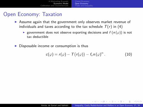
Closed EconomyOpen EconomyTrade and Inequality
Open Economy: TaxationI Assume again that the government only observes market revenue of
individuals and taxes according to the tax schedule T (r) in (4)
I government does not observe exporting decisions and f (n (ϕ)) is nottax deductible
I Disposable income or consumption is thus
c(ϕ) = r(ϕ)− T(r(ϕ)
)− fxn (ϕ)α . (10)
I Agents now choose labor input `(ϕ) and market access investmentn(ϕ) to maximize utility (7) given the revenue function (6) andbudget constraint (10)
I Given symmetry, goods market clearing imposes
Q =
(∫ 1
0
Υ1−βn(ϕ)y(ϕ)β
)1/β
(11)
Antras, de Gortari and Itskhoki Inequality, Costly Redistribution and Welfare in an Open Economy 27 / 39
A Motivating ExampleEconomic Model
Calibration and Counterfactuals
Closed EconomyOpen EconomyTrade and Inequality
Open Economy: TaxationI Assume again that the government only observes market revenue of
individuals and taxes according to the tax schedule T (r) in (4)
I government does not observe exporting decisions and f (n (ϕ)) is nottax deductible
I Disposable income or consumption is thus
c(ϕ) = r(ϕ)− T(r(ϕ)
)− fxn (ϕ)α . (10)
I Agents now choose labor input `(ϕ) and market access investmentn(ϕ) to maximize utility (7) given the revenue function (6) andbudget constraint (10)
I Given symmetry, goods market clearing imposes
Q =
(∫ 1
0
Υ1−βn(ϕ)y(ϕ)β
)1/β
(11)
Antras, de Gortari and Itskhoki Inequality, Costly Redistribution and Welfare in an Open Economy 27 / 39

A Motivating ExampleEconomic Model
Calibration and Counterfactuals
Closed EconomyOpen EconomyTrade and Inequality
Trade and InequalityI Result: Trade increases inequality of revenues and utilities
c (ϕ)
Q∝
ϕβ(1+ε)(1−φ)
1+εφ , ϕ < ϕx1 ,
Υ(1−β)(1+ε)(1−φ)
1+εφ
1 ϕβ(1+ε)(1−φ)
1+εφ , ϕ < ϕx2,
......
Υ(1−β)(1+ε)(1−φ)
1+εφ
N ϕβ(1+ε)(1−φ)
1+εφ ϕ ≥ ϕxN
Υn = 1+nτ−β
1−β
I Two limiting cases:
I no agent exports (ϕx1 →∞)I all agents export (ϕxN → ϕmin)
c (ϕ)
Q=
caut (ϕ)
Qaut∝ ϕ
β(1+ε)(1−φ)1+εφ
Antras, de Gortari and Itskhoki Inequality, Costly Redistribution and Welfare in an Open Economy 28 / 39

A Motivating ExampleEconomic Model
Calibration and Counterfactuals
Closed EconomyOpen EconomyTrade and Inequality
Trade and Inequality (cont.)I Trade increases relative sale revenue of high-ability households but
reduces that of low-ability households
Productivity0 100 200 300 400 500 600 700 800 900 1000
Rel
ativ
e R
even
ues,
r/R
0
1
2
3
4
5
6
AutarkyOpen Economy
Antras, de Gortari and Itskhoki Inequality, Costly Redistribution and Welfare in an Open Economy 29 / 39

A Motivating ExampleEconomic Model
Calibration and Counterfactuals
Closed EconomyOpen EconomyTrade and Inequality
Trade and Inequality (cont.)
Variable Trade Cost =1 1.5 2 2.5
1
1.02
1.04
1.06
1.08
1.1
1.12Gini Ratio, N=10
Variable Trade Cost =1 1.5 2 2.5
1.2
1.3
1.4
1.5
1.6
1.7
1.8
1.9Variance(R/mean(R)) Ratio, N=10
Variable Trade Cost =1 1.5 2 2.5
1
1.005
1.01
1.015
1.02
1.025
1.03
1.035Gini Ratio, N=1
Pre-TaxPost-Tax
Variable Trade Cost =1 1.5 2 2.5
1.01
1.02
1.03
1.04
1.05
1.06
1.07Variance(R/mean(R)) Ratio, N=1
Antras, de Gortari and Itskhoki Inequality, Costly Redistribution and Welfare in an Open Economy 30 / 39

A Motivating ExampleEconomic Model
Calibration and Counterfactuals
CalibrationCalibrated Welfarist CorrectionCalibrated Costly Redistribution Correction
Calibration and Counterfactuals: Road Map
I We first calibrate the model to 2007 U.S. data (trade share, incomedistribution, tax progressivity)
I We then explore the implication of a move to autarky on
1. Aggregate Income
2. Income Inequality
I We use the model to gauge the quantitative importance of the twocorrections developed above
1. How large are the gains from trade for different degrees of inequalityaversion?
2. How large would the gains from trade be in the absence of costlyredistribution (i.e., φ = 0)?
Antras, de Gortari and Itskhoki Inequality, Costly Redistribution and Welfare in an Open Economy 31 / 39

A Motivating ExampleEconomic Model
Calibration and Counterfactuals
CalibrationCalibrated Welfarist CorrectionCalibrated Costly Redistribution Correction
Calibration
I Hold the following parameters fixed
1. Elasticity of substitution = 4 (β = 3/4) as before
2. Iceberg trade costs (τ = 1.83)
I Melitz and Redding (2014), Anderson and Van Wincoop (2004)
3. Number of countries (N = 10)
I U.S. roughly 10-15% of world GDP; results not too sensitive to Nabove 5
I Set baseline fixed cost fx to match a U.S. trade share of 0.14
I Set convexity of fixed costs to either α = 1 or α = 3 (consistentwith preliminary estimates exploiting cross-section of U.S. exports)
Antras, de Gortari and Itskhoki Inequality, Costly Redistribution and Welfare in an Open Economy 32 / 39
A Motivating ExampleEconomic Model
Calibration and Counterfactuals
CalibrationCalibrated Welfarist CorrectionCalibrated Costly Redistribution Correction
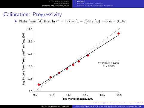
Calibration: ProgressivityI Note from (4) that ln rd = ln k + (1− φ) ln r (ϕ) =⇒ φ = 0.147
y = 0.853x + 1.661R² = 0.995
9.5
10.5
11.5
12.5
13.5
14.5
9.5 10.5 11.5 12.5 13.5 14.5
Log Income After Taxes and Transfers, 2007
Log Market Income, 2007
Antras, de Gortari and Itskhoki Inequality, Costly Redistribution and Welfare in an Open Economy 33 / 39

A Motivating ExampleEconomic Model
Calibration and Counterfactuals
CalibrationCalibrated Welfarist CorrectionCalibrated Costly Redistribution Correction
Calibrated Welfare Gains from Trade and Inequality
I Calibrated welfare gains from trade are higher, the higher is thelabor supply elasticity ε (Arkolakis and Esposito, 2014)
I But relative to autarky trade induces more inequality when ε is high
Gains from Trade Increase in Gini Coefficient
Labor supply elasticity α = 1 α = 3 α = 1 α = 3
ε = 0 4.86% 4.02% 2.31% 1.70%
ε = 0.1 5.52% 4.54% 2.44% 1.81%
ε = 0.25 6.54% 5.36% 2.64% 1.95%
ε = 0.5 8.31% 6.77% 2.92% 2.17%
ε = 0.75 10.40% 8.32% 3.16% 2.35%
ε = 1 12.41% 9.89% 3.36% 2.51%
ε = 1.5 16.72% 13.21% 3.72% 2.78%
Antras, de Gortari and Itskhoki Inequality, Costly Redistribution and Welfare in an Open Economy 34 / 39

A Motivating ExampleEconomic Model
Calibration and Counterfactuals
CalibrationCalibrated Welfarist CorrectionCalibrated Costly Redistribution Correction
Welfarist CorrectionI Welfarist correction is higher, the higher is risk/inequality aversion ρ
and the lower is the labor supply elasticity ε
I With log utility (ρ = 1) and a labor supply elasticity of ε = 0.5,welfare gains are 21% lower for both α = 1 and α = 3
0.60
0.65
0.70
0.75
0.80
0.85
0.90
0.95
1.00
0 0.1 0.25 0.5 0.75 1 2
Degree of Risk/Inequality Aversion ()
Welfarist Adjustment ()
0.60
0.65
0.70
0.75
0.80
0.85
0.90
0.95
1.00
0 0.1 0.25 0.5 0.75 1 2
Degree of Risk/Inequality Aversion ()
Welfarist Adjustment (=3)
Antras, de Gortari and Itskhoki Inequality, Costly Redistribution and Welfare in an Open Economy 35 / 39

A Motivating ExampleEconomic Model
Calibration and Counterfactuals
CalibrationCalibrated Welfarist CorrectionCalibrated Costly Redistribution Correction
Costly Redistribution CorrectionI Costly redistribution correction is higher, the higher is the labor
supply elasticity ε
I When ε = 0.5, welfare gains are 21% lower for α = 1 and 16% lowerfor α = 3
0.60
0.65
0.70
0.75
0.80
0.85
0.90
0.95
1.00
Elasticity of Labor Supply
Costly Redistribution Correction ( =0)
Antras, de Gortari and Itskhoki Inequality, Costly Redistribution and Welfare in an Open Economy 36 / 39

A Motivating ExampleEconomic Model
Calibration and Counterfactuals
CalibrationCalibrated Welfarist CorrectionCalibrated Costly Redistribution Correction
Nonparametric versus Lognormal CaseI Lognormal underpredicts costly redistribution correction, especially
for high ε (underpredicts the behavior of the right tail)
0.65
0.7
0.75
0.8
0.85
0.9
0.95
1
0.65 0.7 0.75 0.8 0.85 0.9 0.95 1
Nonparam
etric Distribution
Lognormal Distribution
Nonparametric vs. Lognormal Costly Redistribution Correction ( =0)
Antras, de Gortari and Itskhoki Inequality, Costly Redistribution and Welfare in an Open Economy 37 / 39
A Motivating ExampleEconomic Model
Calibration and Counterfactuals
CalibrationCalibrated Welfarist CorrectionCalibrated Costly Redistribution Correction
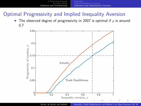
Optimal Progressivity and Implied Inequality AversionI The observed degree of progressivity in 2007 is optimal if ρ is around
0.7
Inequality aversion, ρ0 0.2 0.4 0.6 0.8 1
Progressivityoftaxation,φ
0
0.05
0.1
0.15
0.2
0.25
Trade Equilibrium
Autarky
Antras, de Gortari and Itskhoki Inequality, Costly Redistribution and Welfare in an Open Economy 38 / 39

A Motivating ExampleEconomic Model
Calibration and Counterfactuals
CalibrationCalibrated Welfarist CorrectionCalibrated Costly Redistribution Correction
ConclusionsI Trade-induced inequality is partly mitigated via a progressive income
tax system
I Still, compensation is not full so trade induces an increase in thedistribution of disposable income
I Is it so clear that the Kaldor-Hicks principle is free of valuejudgements in that case?
I Income taxation induces behavioral responses that affect theaggregate income response to trade integration
I Shouldn’t the Kaldor-Hicks principle adjust for this “leaky bucket”effect?
I In this paper, we have developed welfarist and costly redistributioncorrections to standard measures of the gains from trade integration
I Under plausible parameter values, these corrections are nonneglibleand eliminate about one-fifth of the (static) gains from trade
Antras, de Gortari and Itskhoki Inequality, Costly Redistribution and Welfare in an Open Economy 39 / 39