trade, inequality and costly redistribution · trade, inequality and costly redistribution pol antr...

Trade, Inequality andCostly Redistribution

Pol Antras Alonso de Gortari Oleg ItskhokiHarvard Harvard Princeton

ILO SymposiumSeptember 2015

1 / 30

Introduction

• International trade raises real income but also increasesinequality and makes some worse off

• Standard approach to demonstrating and quantifying thegains from trade largely ignore trade-induced inequality

— Kaldor-Hicks compensation principle

• Two issues with this approach:

1 How much compensation/redistribution actually takes place?

2 Is this redistribution costless, as the Kaldor-Hicks approachassumes?

• These issue are relevant not just for trade, but also fortechnology adoption etc.

2 / 30

This Paper

• We study quantitatively welfare implications of trade in amodel where:

1 trade leads to an increase in inequality

2 redistribution requires distortionary taxation(e.g., due to informational constraints, as in Mirrlees)

3 despite progressive tax system, trade still increases inequalityin after-tax incomes

• We propose two types of adjustment to standard welfaremeasures:

1 Welfarist correction: taking into account inequality-aversionof society (or risk-adjustment under the veil of ignorance)

2 Costly-redistribution correction: capturing behavioralresponses to trade-induced shifts across marginal tax rates

3 / 30

Motivating Figure

1975 1980 1985 1990 1995 2000 2005 20100.9

1

1.1

1.2

1.3

1.4

1.5

1.6

1.7Real Income in the United States (1979-2007)

Mean IncomeMedian Income

1.74% versus 0.47% annualized annual growth

4 / 30

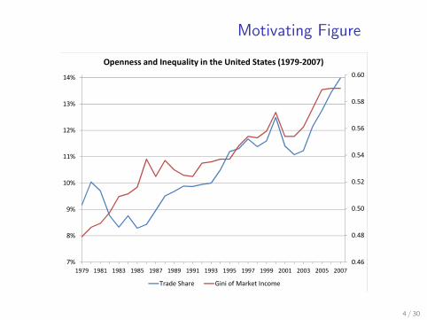
Motivating Figure

0.46

0.48

0.50

0.52

0.54

0.56

0.58

0.60

7%

8%

9%

10%

11%

12%

13%

14%

1979 1981 1983 1985 1987 1989 1991 1993 1995 1997 1999 2001 2003 2005 2007

Openness and Inequality in the United States (1979‐2007)

Trade Share Gini of Market Income

4 / 30

Building Blocks and Related Literature• Trade models with heterogeneous workers

— Itskhoki (2008)— matching/sorting models (see Grossman, and Costinot and

Vogel for surveys)— models with imperfect labor markets (Helpman, Itskhoki,

Redding, and others)

• Gains from trade and costly redistribution: Dixit and Norman(1986), Rodrik (1992), Spector (2001), Naito (2006)

• Welfarist approach: Bergson (1938), Samuelson (1947),Diamond & Mirlees (1971), Saez more recently

• Costly-redistribution:— Kaplow (2008), Hendren (2014)— Nonlinear tax system as in Heathcote, Storesletten and

Violante (2014)— Model calibrated to fit 2007 U.S. data on income distribution

from IRS public records

5 / 30

Road Map

1 A Motivating Example

2 Open Economy Model

3 Calibration

4 Counterfactuals: Inequality and the Gains from Trade

6 / 30

MOTIVATING EXAMPLE

7 / 30

The Kaldor-Hicks Principle• Consider an economy with a unit measure of individuals with

ability ϕ ∼ Hϕ earning market income rϕ ∼ Fr

• We want to evaluate a shift of income distribution Fr → F ′r

• The compensating variation vϕ for each individual:

u(rϕ) = u(r ′ϕ + vϕ) ⇒ vϕ = rϕ − r ′ϕ

• Hence:

−∫

vϕdHϕ =

∫r ′ϕdHϕ −

∫rϕdHϕ

=

∫rdF ′r −

∫rdFr = R ′ − R

• Kaldor-Hicks Gains = Aggregate Real Income Growth

GKH =R ′ − R

R≡ µ

7 / 30

The Kaldor-Hicks PrinciplePros and Cons

• Principle does not rely on interpersonal comparisons of utility:

— indirect utility can be heterogeneous across agents

— result relies on ordinal rather than cardinal preferences

— notion of efficiency argued to be free of value judgements

• What if redistribution does not take place?

— under the veil of ignorance, agents see a probability distributionover potential outcomes (need cardinal preferences)

— risk aversion ≈ inequality aversion

• Even if some redistribution takes place, whenever it is costly,shouldn’t ∆W /W reflect those costs?

— Dixit and Norman (1986) showed that ∆W /W > 0 using acourse set of taxes, but by how much is ∆W /W diminished?

8 / 30

A Constant-Elasticity ModelClosed Economy

• A unit measure of individuals with CRRA-GHH utility:

U(c , `) =1

1 + ρ

(c − 1

γ`γ)

• Each individual produces a task according to y = ϕ`, ϕ ∼ Hϕ

• This translates into market income r = Q1−βyβ, Q =∫rϕdHϕ

• Consumption equals after-tax income: show data

c = r − T (r) = kr1−φ

• Government runs balanced budget g =G

Q= 1− k

∫r1−φϕ dHϕ∫rϕdHϕ

• In constant-elasticity model, rϕ ∝ ϕβ(1+ε)1+εφ , where ε ≡ β

γ − β

9 / 30

A Constant-Elasticity ModelClosed Economy

• A unit measure of individuals with CRRA-GHH utility:

U(c , `) =1

1 + ρ

(c − 1

γ`γ)

• Each individual produces a task according to y = ϕ`, ϕ ∼ Hϕ

• This translates into market income r = Q1−βyβ, Q =∫rϕdHϕ

• Consumption equals after-tax income: show data

c = r − T (r) = kr1−φ

• Government runs balanced budget g =G

Q= 1− k

∫r1−φϕ dHϕ∫rϕdHϕ

• In constant-elasticity model, rϕ ∝ ϕβ(1+ε)1+εφ , where ε ≡ β

γ − β9 / 30

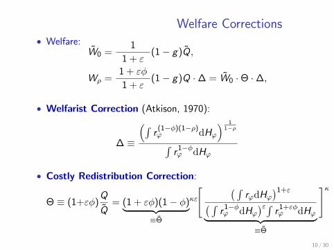
Welfare Corrections• Welfare:

W0 =1

1 + ε(1− g)Q,

Wρ =1 + εφ

1 + ε(1− g)Q ·∆ = W0 ·Θ ·∆,

• Welfarist Correction (Atkison, 1970):

∆ ≡

(∫r

(1−φ)(1−ρ)ϕ dHϕ

) 11−ρ∫

r1−φϕ dHϕ

• Costly Redistribution Correction:

Θ ≡ (1+εφ)Q

Q= (1 + εφ)(1− φ)︸︷︷︸

≡Θ

κε

[ ( ∫rϕdHϕ

)1+ε( ∫r1−φϕ dHϕ

)ε∫r1+εφϕ dHϕ︸︷︷︸

≡Θ

]κ

10 / 30

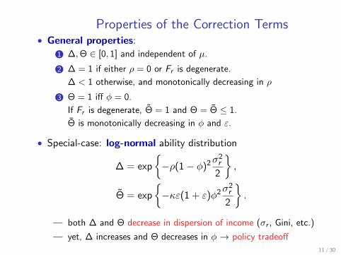
Properties of the Correction Terms• General properties:

1 ∆,Θ ∈ [0, 1] and independent of µ.

2 ∆ = 1 if either ρ = 0 or Fr is degenerate.

∆ < 1 otherwise, and monotonically decreasing in ρ

3 Θ = 1 iff φ = 0.

If Fr is degenerate, Θ = 1 and Θ = Θ ≤ 1.

Θ is monotonically decreasing in φ and ε.

• Special-case: log-normal ability distribution

∆ = exp

{−ρ(1− φ)2σ

2r

2

},

Θ = exp

{−κε(1 + ε)φ2σ

2r

2

}.

— both ∆ and Θ decrease in dispersion of income (σr , Gini, etc.)

— yet, ∆ increases and Θ decreases in φ → policy tradeoff

11 / 30

Corrections for Welfare Gains

• GDP growth rates:

µ =Q ′ − Q

Q,

µ =Q ′ − Q

Q= G

• Welfarist correction:

GW ≡ ∆Wρ

Wρ= (1 + µ)

∆′

∆− 1

• Costly redistribution correction:

µ = (1 + µ)Θ′

Θ− 1

12 / 30

Look at the dataGrowth corrections for US, 1979–2007

Welfare correction: GW /µ ∼ ∆′/∆ρ = 0.5 1 2

Non-parametric 0.89 0.80 −0.08Log-normal 0.90 0.80 0.60

CR correction: µ/µ ∼ Θ′/Θε = 0.5 1 2

Non-parametric 1.04 1.14 1.98Log-normal 1.06 1.27 (µ < 0)

— Recall that annualized µ = 1.74% over 1979–2007,

— inequality increased

— but progressively (φ) decreased

13 / 30

Policy Tradeoff for US, 1979–2007

• In logs: logWρ = log W0 +

≡−θ︷︸︸︷log Θ +

≡−δ︷︸︸︷log ∆

/ Contribution (Inequality)0.1 0.15 0.2 0.25 0.3 0.35 0.4 0.45 0.5 0.55 0.6

3 C

ontr

ibut

ion

(Tax

atio

n)

0.06

0.07

0.08

0.09

0.1

0.11

0.12(/ ,3) Phase Diagram, rho=0.5, eps=0.5


3 C

ontr

ibut

ion

(Tax

atio

n)

0.06

0.07

0.08

0.09

0.1

0.11



3 C

ontr

ibut

ion

(Tax

atio

n)

0.06

0.07

0.08

0.09

0.1

0.11


14 / 30

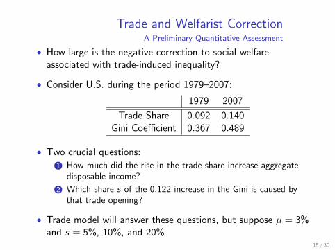
Trade and Welfarist CorrectionA Preliminary Quantitative Assessment

• How large is the negative correction to social welfareassociated with trade-induced inequality?

• Consider U.S. during the period 1979–2007:

1979 2007

Trade Share 0.092 0.140Gini Coefficient 0.367 0.489

• Two crucial questions:

1 How much did the rise in the trade share increase aggregatedisposable income?

2 Which share s of the 0.122 increase in the Gini is caused bythat trade opening?

• Trade model will answer these questions, but suppose µ = 3%and s = 5%, 10%, and 20%

15 / 30

Welfarist CorrectionA Preliminary Quantitative Assessment

• It does not take an awful lot of inequality aversion to generatesignificant downward corrections to gains from trade

Table 1. Social Welfarist Inequality Correction to Welfare Effects of Trade Integration

Pareto Correction Lognormal CorrectionContribution of Trade to Inequality Contribution of Trade to Inequality

s = 5% s = 10% s = 20% s = 5% s = 10% s = 20%Inequality Aversion (1) (2) (3) (4) (5) (6)

ρ = 0 3.00% 3.00% 3.00% 3.00% 3.00% 3.00%ρ = 0.1 2.85% 2.69% 2.36% 2.91% 2.83% 2.65%ρ = 0.25 2.67% 2.33% 1.64% 2.79% 2.57% 2.12%ρ = 0.5 2.46% 1.92% 0.80% 2.57% 2.14% 1.25%ρ = 0.75 2.32% 1.63% 0.23% 2.36% 1.72% 0.39%ρ = 1 2.22% 1.43% -0.18% 2.15% 1.29% -0.46%ρ = 2 1.98% 0.96% -1.08% 1.31% -0.39% -3.81%

1

16 / 30

ECONOMIC MODEL

17 / 30

Open EconomyEnvironment

• Consider a world economy with N + 1 symmetric regions

• Households can market their output locally or in any of theother N regions

• Trade/Offshoring involves two types of additional costs

1 Variable iceberg trade cost τ

2 Fixed cost of market access f (n) increasing in the number n offoreign markets served. We adopt f (n) = fnα

• Household income

rϕ = Υ1−βnϕ Q1−βyβϕ , where Υnϕ = 1 + nϕτ

− β1−β

• Taxation: the government does not observe export decisionsand f (n) is not tax deductible: cϕ = kr1−φ

ϕ − fnαϕ

17 / 30

Trade and Inequality• Trade increases relative revenues of high-ability households

(due to market access), but reduces that of low-abilityhouseholds (due to foreign competition)

Productivity0 100 200 300 400 500 600 700 800 900 1000

Rel

ativ

e R

even

ues,

r/R

0

1

2

3

4

5

6

AutarkyOpen Economy

18 / 30

Trade and Inequality

Variable Trade Cost =1 1.5 2 2.5

1

1.02

1.04

1.06

1.08

1.1

1.12Gini Ratio, N=10


1.2

1.3

1.4

1.5

1.6

1.7

1.8

1.9Variance(R/mean(R)) Ratio, N=10


1

1.005

1.01

1.015

1.02

1.025

1.03

1.035Gini Ratio, N=1

Pre-TaxPost-Tax


1.01

1.02

1.03

1.04

1.05

1.06

1.07Variance(R/mean(R)) Ratio, N=1

19 / 30

CALIBRATION ANDCOUNTERFACTUALS

20 / 30

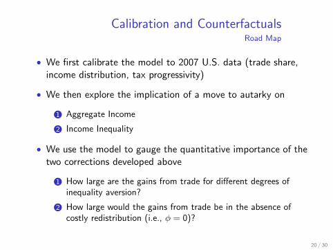
Calibration and CounterfactualsRoad Map

• We first calibrate the model to 2007 U.S. data (trade share,income distribution, tax progressivity)

• We then explore the implication of a move to autarky on

1 Aggregate Income

2 Income Inequality

• We use the model to gauge the quantitative importance of thetwo corrections developed above

1 How large are the gains from trade for different degrees ofinequality aversion?

2 How large would the gains from trade be in the absence ofcostly redistribution (i.e., φ = 0)?

20 / 30

Calibration

• Hold the following parameters fixed

1 Elasticity of substitution = 4 (β = 3/4)

• BEJK (2003), Broda and Weinstein (2006), Antras, Fort and Tintelnot (2014)

2 Iceberg trade costs (τ = 1.83)

• Anderson and Van Wincoop (2004), Melitz and Redding (2014)

3 Number of countries (N = 10)

• U.S. roughly 10-15% of world manufacturing; results not toosensitive to N above 5

• Set baseline fixed cost f to match a U.S. trade share of 0.14

• Set convexity of fixed costs to either α = 1 or α = 3(consistent with preliminary estimates using U.S. exports)

• Labor supply elasticity: experiment with various values for γbetween γ = 10000 (or ε ' 0) and γ = 5/3 (or ε = 1.5)

21 / 30

Calibration: Progressivity

• We set φ = 0.147, consistent with 2007 income data:

y = 0.853x + 1.661R² = 0.995

9.5

10.5

11.5

12.5

13.5

14.5

9.5 10.5 11.5 12.5 13.5 14.5

Log Income After Taxes and

Transfers, 200

7

Log Market Income, 2007

22 / 30

Calibration: Distribution of Ability

• Use 2007 U.S. Individual Income Tax Public Use Sample

• approximately 2.5 million anonymized tax returns

• use NBER weights to ensure this is a representative sample

• we map market income to adjusted gross income in line 37 ofIRS Form 1040

• We follow two types of approaches:

1 Nonparametric approach: given other parameter values, onecan recover the ϕ’s from the observed distribution of adjustedgross income

2 Parametric approach: assume that ϕ ∼ LogNormal(µ, σ) andcalibrate µ and σ to match the mean and the Gini coefficientof adjusted gross income

23 / 30

Parametric vs. Non-Parametric Approach

• Lognormal provides a reasonably good approximation, but itdoes a poor fit for the right-tail of the distribution, whichlooks Pareto

log(R)6 8 10 12

0

0.1

0.2

0.3

0.4

0.5

0.6

0.7

0.8

0.9

1Income Distribution

NonparametricLognormalData

R #1050 2 4 6 8 10

1

1.2

1.4

1.6

1.8

2

2.2

2.4

2.6Empirical Pareto Coefficient

24 / 30

Gains from Trade and Inequality

• Calibrated welfare gains from trade are higher, the higher isthe labor supply elasticity ε

• But relative to autarky trade induces more inequality when εis high

Gains from Trade Increase in Gini Coefficient

Labor supply elasticity α = 1 α = 3 α = 1 α = 3

ε = 0 4.86% 4.02% 2.31% 1.70%ε = 0.1 5.52% 4.54% 2.44% 1.81%ε = 0.25 6.54% 5.36% 2.64% 1.95%ε = 0.5 8.31% 6.77% 2.92% 2.17%ε = 0.75 10.40% 8.32% 3.16% 2.35%ε = 1 12.41% 9.89% 3.36% 2.51%ε = 1.5 16.72% 13.21% 3.72% 2.78%

25 / 30

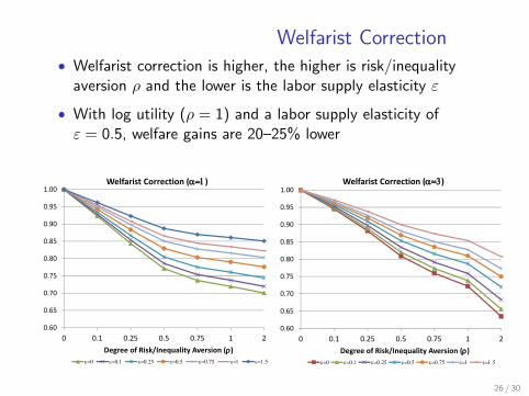
Welfarist Correction• Welfarist correction is higher, the higher is risk/inequality

aversion ρ and the lower is the labor supply elasticity ε

• With log utility (ρ = 1) and a labor supply elasticity ofε = 0.5, welfare gains are 20–25% lower

0.60

0.65

0.70

0.75

0.80

0.85

0.90

0.95

1.00

0 0.1 0.25 0.5 0.75 1 2Degree of Risk/Inequality Aversion ()

Welfarist Correction ()

0.60

0.65

0.70

0.75

0.80

0.85

0.90

0.95

1.00

0 0.1 0.25 0.5 0.75 1 2Degree of Risk/Inequality Aversion ()

Welfarist Correction ()

26 / 30

Costly Redistribution Correction

• Costly redistribution correction is higher, the higher is thelabor supply elasticity ε

• When ε = 0.5, welfare gains are 15–20% lower

0.60

0.65

0.70

0.75

0.80

0.85

0.90

0.95

1.00

Elasticity of Labor Supply

Costly Redistribution Correction ( =0)

27 / 30

Welfare gains from trade

Export share of revenues0 0.05 0.1 0.15 0.2 0.25

Incomegrowth

1

1.05

1.1

1.15

1.2

1.25

Median

Mean

Welfare

Undistorted Mean

28 / 30

OPTIMAL PROGRESSIVITY

29 / 30

Progressivity and Inequality Aversion• Optimal progressively is lower in open economy ⇒ greater

inequality increase if φ is adjusted

Progressivity of taxation, φ0 0.05 0.1 0.15 0.2 0.25 0.3 0.35 0.4

Socialwelfare,W

1

1.05

1.1

1.15

1.2

1.25

Autarky

Trade Equilibrium

φ∗

Tφ∗

A

29 / 30

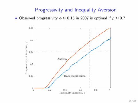
Progressivity and Inequality Aversion

• Observed progressivity φ ≈ 0.15 in 2007 is optimal if ρ ≈ 0.7

Inequality aversion, ρ0 0.2 0.4 0.6 0.8 1

Progressivityoftaxation,φ

0

0.05

0.1

0.15

0.2

0.25

Trade Equilibrium

Autarky

29 / 30

Progressivity and Inequality Aversion

• Optimal progressively is lower in open economy ⇒ greaterinequality increase if φ is adjusted


Giniofrevenues

0.52

0.54

0.56

0.58

0.6

0.62

0.64

0.66

Autarky

Trade Equilibrium

φ∗

Tφ∗

A


Meanrevenues

0.5

0.6

0.7

0.8

0.9

1

1.1

1.2

Autarky

Trade Equilibrium

φ∗

Tφ∗

A

29 / 30

Conclusions

• Trade-induced inequality is partly mitigated via a progressiveincome tax system

• Still, compensation is not full so trade induces an increase inthe inequality of disposable income

−→ should we measure gains using average income or adjust forinequality?

• Income taxation induces behavioral responses that affect theaggregate income response to trade integration

−→ should we adjust for this “leaky bucket” effect?

• We developed welfarist and costly redistribution corrections tostandard measures of the gains from trade

• Under plausible parameter values, these corrections arenonneglible and eliminate about one-fifth of the gains

30 / 30

APPENDIX

31 / 30

On the Shape of the Tax Schedule• The tax schedule might seem ad hoc, but it fits U.S. data

remarkably well: log rdϕ = log k + (1− φ) log rϕ

y = 0.818x + 2.002 R² = 0.988

9

10

11

12

13

14

9 10 11 12 13 14

Log

Inco

me

Afte

r Tax

es a

nd T

rans

fers

Log Market Income

CBO data, percentiles of income distribution 1979–2010 (similar fit with PSID)

back to slides

32 / 30

On the Shape of the Tax ScheduleOver Time

0.1

.2.3

.4.5

φ

1980 1990 2000 2010Year

Degree of Progressivity φ

back to slides33 / 30

trade, inequality and costly redistribution · trade, inequality and costly redistribution pol antr...

Documents