Inf2b Learning and DataLecture 3: Clustering and data visualisation

Hiroshi Shimodaira(Credit: Iain Murray and Steve Renals)

Centre for Speech Technology Research (CSTR)School of Informatics

University of Edinburghhttp://www.inf.ed.ac.uk/teaching/courses/inf2b/

https://piazza.com/ed.ac.uk/spring2018/infr08009learning

Office hours: Wednesdays at 14:00-15:00 in IF-3.04

Jan-Mar 2018

Inf2b Learning and Data: Lecture 3 Clustering and data visualisation 1

Today’s Schedule

1 What is clustering

2 K -means clustering

3 Hierarchical clustering

4 Example – unmanned ground vehicle navigation

5 Dimensionality reduction with PCA and data visualisation

6 Summary

Inf2b Learning and Data: Lecture 3 Clustering and data visualisation 2

Clustering

Clustering: partition a data set into meaningful or usefulgroups, based on distances between data points

Clustering is an unsupervised process — the data itemsdo not have class labels

Why cluster?

Interpreting data Analyse and describe a situation byautomatically dividing a data set intogroupings

Compressing data Represent data vectors by their clusterindex — vector quantisation

Inf2b Learning and Data: Lecture 3 Clustering and data visualisation 3

Clustering

“Human brains are good at finding regularities in data.One way of expressing regularity is to put a set of objectsinto groups that are similar to each other. For exam-ple, biologists have found that most objects in the nat-ural world fall into one of two categories: things thatare brown and run away, and things that are green anddon’t run away. The first group they call animals, andthe second, plants.”

Recommended reading: David MacKay textbook, p284–

http://www.inference.phy.cam.ac.uk/mackay/itila/

Inf2b Learning and Data: Lecture 3 Clustering and data visualisation 4

Visualisation of film review users

MovieLens data set(http://grouplens.org/datasets/movielens/)C ≈ 1000 users, M ≈ 1700 movies

-60

-40

-20

0

20

40

60

-60 -40 -20 0 20 40 60

2D plot of users based on rating similarity

Inf2b Learning and Data: Lecture 3 Clustering and data visualisation 5

Application of clustering

Face clusteringdoi: 10.1109/CVPR.2013.450LHI-Animal-Face dataset

Image segmentationhttp:

//dx.doi.org/10.1093/bioinformatics/btr246

Document clusteringThesaurus generation

Temporal Clustering of Human Behaviourhttp://www.f-zhou.com/tc.html

Inf2b Learning and Data: Lecture 3 Clustering and data visualisation 7

A two-dimensional space

http://homepages.inf.ed.ac.uk/imurray2/teaching/oranges_and_lemons/

Inf2b Learning and Data: Lecture 3 Clustering and data visualisation 11

The Unsupervised data

4

6

8

10

6 8 10

height/cm

width/cmInf2b Learning and Data: Lecture 3 Clustering and data visualisation 12

Manderins

4

6

8

10

6 8 10

height/cm

width/cmInf2b Learning and Data: Lecture 3 Clustering and data visualisation 13

Navel oranges

4

6

8

10

6 8 10

height/cm

width/cmInf2b Learning and Data: Lecture 3 Clustering and data visualisation 14

Spanish jumbo oranges

4

6

8

10

6 8 10

height/cm

width/cmInf2b Learning and Data: Lecture 3 Clustering and data visualisation 15

Belsan lemons

4

6

8

10

6 8 10

height/cm

width/cmInf2b Learning and Data: Lecture 3 Clustering and data visualisation 16

Some other lemons

4

6

8

10

6 8 10

height/cm

width/cmInf2b Learning and Data: Lecture 3 Clustering and data visualisation 17

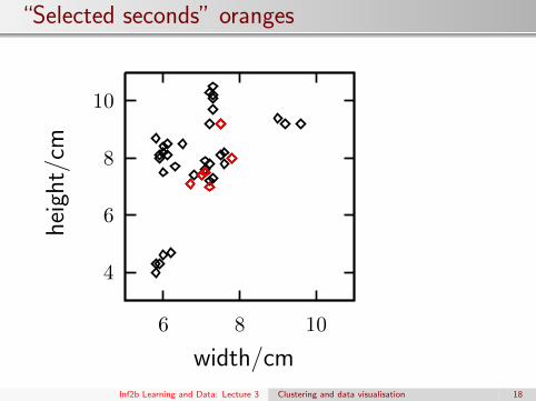
“Selected seconds” oranges

4

6

8

10

6 8 10

height/cm

width/cmInf2b Learning and Data: Lecture 3 Clustering and data visualisation 18

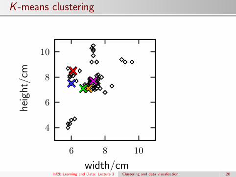
K -means clustering

A simple algorithm to find clusters:

1 Pick K random points as cluster centre positions

2 Assign each point to its nearest centre∗

3 Move each centre to mean of its assigned points

4 If centres moved, goto 2.

∗ In the unlikely event of a tie, break tie in some way.For example, assign to the centre with smallest index in

memory.

Inf2b Learning and Data: Lecture 3 Clustering and data visualisation 19

K -means clustering

10

8

6

4

1086

height/cm

width/cmInf2b Learning and Data: Lecture 3 Clustering and data visualisation 20

Evaluation of clustering

One way to measure the quality of a k-means clusteringsolution is by a sum-squared error function, i.e. the sumof squared distances of each point from its cluster centre.

Let zkn = 1 if the point xn belongs to cluster k andzkn = 0 otherwise. Then:

E =K∑

k=1

N∑n=1

zkn‖xn −mk‖2xn = (xn1, . . . , xnD)T

mk = (mk1, . . . ,mkD)T

‖·‖ : Euclidean (L2) norm

where mk is the centre of cluster k .

Sum-squared error is related to the variance — thusperforming k-means clustering to minimise E issometimes called minimum variance clustering.

This is a within-cluster error function — it does notinclude a between clusters term

Inf2b Learning and Data: Lecture 3 Clustering and data visualisation 21

Theory of K -means clustering

If assignments don’t change, algorithm terminates.

Can assignments cycle, never terminating?

Convergence proof technique: find a Lyapunovfunction L, that is bounded below and cannot increase.L = sum of square distances between points and centres

NB: E (t+1) ≤ E (t)

K -means is an optimisation algorithm for L.Local optima are found, i.e. there is no guarantee offinding global optimum. Running multiple times andusing the solution with best L is common.

Inf2b Learning and Data: Lecture 3 Clustering and data visualisation 22

How to decide K?

The sum-squared error decreases as K increases( E → 0 as K → N)

We need another measure?!

0 2 4 6 8 100

0.5

1

1.5

2

2.5

3

3.5

K

Sum

square

d e

rror

6 8 103

4

5

6

7

8

9

10

11

width [cm]

heig

ht [m

]

Inf2b Learning and Data: Lecture 3 Clustering and data visualisation 23

Failures of K -means (e.g. 1)

3

5

7

3 5 7

Large clouds pull small clusters off-centre

Inf2b Learning and Data: Lecture 3 Clustering and data visualisation 24

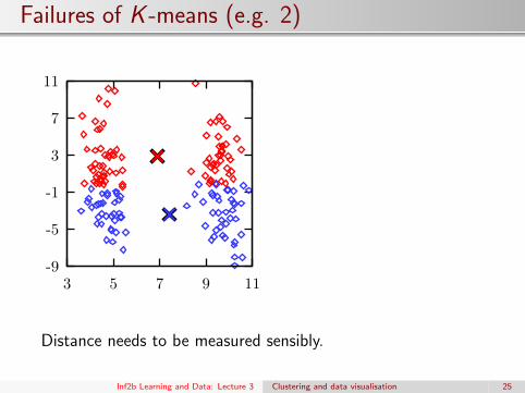
Failures of K -means (e.g. 2)

-9

-5

-1

3

7

11

3 5 7 9 11

Distance needs to be measured sensibly.

Inf2b Learning and Data: Lecture 3 Clustering and data visualisation 25

Clustering clustering methods (NE)

K -means clustering is not the only method for clusteringdata

See:http://en.wikipedia.org/wiki/Cluster_analysis

Inf2b Learning and Data: Lecture 3 Clustering and data visualisation 26

Hierarchical clustering (NE)

Form a ‘dendrogram’ / binary tree with data at leaves

Bottom-up / Agglomerative:

Repeatedly merge closest groups of points

Often works well. Expensive: O(N3)

Top-down / Divisive:

Recursively split groups into two (e.g. with k-means)

Early choices might be bad.

Much cheaper! ∼ O(N2) or O(N2 logN)

More detail:Pattern Classification (2nd ed.), Duda, Hart, Stork. §10.9

Inf2b Learning and Data: Lecture 3 Clustering and data visualisation 27

Bottom-up clustering of the lemon/orange data

0 0.5 1 1.5 2 2.5 3 3.5 4Orange 12Orange 22Orange 18Orange 11Orange 21Orange 14Orange 19Orange 24Orange 10Orange 13Orange 16Orange 15Orange 23Orange 17Orange 20Lemon 31Lemon 35Lemon 36Lemon 32Lemon 40Lemon 34Lemon 38Lemon 39Lemon 33Lemon 37Orange 6Orange 7Orange 8Orange 9

Lemon 27Lemon 29Lemon 25Lemon 28Lemon 30Lemon 26Orange 1Orange 2Orange 3Orange 4Orange 5

inter cluster distance

Hierarchical clustering (centroid−distance)

Inf2b Learning and Data: Lecture 3 Clustering and data visualisation 28

Stanley

Stanford Racing Team; DARPA 2005 challenge

http://robots.stanford.edu/talks/stanley/

Inf2b Learning and Data: Lecture 3 Clustering and data visualisation 30

Inside Stanley

Stanley figures from Thrun et al., J. Field Robotics 23(9):661, 2006.

Inf2b Learning and Data: Lecture 3 Clustering and data visualisation 31

Perception and intelligence

It would look pretty stupid to run off the road,just because the trip planner said so.

Inf2b Learning and Data: Lecture 3 Clustering and data visualisation 32

How to stay on the road?

Classifying road seems hard. Colours and textures change:road appearance in one place may match ditches elsewhere.

Inf2b Learning and Data: Lecture 3 Clustering and data visualisation 33

Clustering to stay on the road

Stanley used a Gaussian mixture model. “Souped up k-means.”

The cluster just in front is road (unless we already failed).

Inf2b Learning and Data: Lecture 3 Clustering and data visualisation 34

Dimensionality reduction and data visualisation

High-dimensional data are difficult to understand andvisualise.Consider dimensionality reduction of data for visualisation

2

1

X

X

X

3

1

2

u

u

Project each sample in 3D onto a 2D plane

2

1

2

1u

u

Y

Y

Inf2b Learning and Data: Lecture 3 Clustering and data visualisation 36

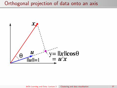
Orthogonal projection of data onto an axis

cosT

||x||y=u x1||u||= =

θθu

x

Inf2b Learning and Data: Lecture 3 Clustering and data visualisation 37

Optimal projection of 2D data onto 1D

X 2

X 1

Y

X 2

X 1

Y

Mapping 2D to 1D: yn = uTxn = u1xn1 + u2xn2

Optimal mapping: maxu

Var (y)

Var (y) = 1N−1

∑Nn=1 (yn − y)2

cf. least squares fitting (linear regression)

Inf2b Learning and Data: Lecture 3 Clustering and data visualisation 38

Principal Component Analysis (PCA)

Mapping D-dimensional data to a principal componentaxis u = (u1, . . . , uD)T that maximises Var (y):

yn = uTxn = u1xn1 + · · ·+ uDxnD NB: ‖u‖ = 1

u is given as the eigen vector with the largest eigen valueof the covariance matrix, S :

S =1

N−1

N∑n=1

(xn−x)(xn−x)T , x =1

N

N∑n=1

xn

Eigen values λi and eigen vectors pi of S :

S pi = λi pi , i = 1, . . . ,D

If λ1 ≥ λ2 ≥ . . . ≥ λD , then u = p1, and Var (y) = λ1

NB: pTi pj = 0, i.e. pi ⊥ pj for i 6= j

pi is normally normalised so that ‖pi‖ = 1.

Inf2b Learning and Data: Lecture 3 Clustering and data visualisation 39

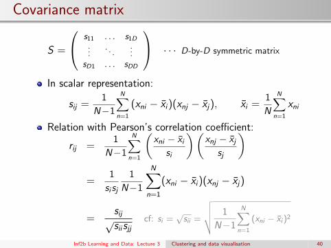
Covariance matrix

S =

s11 . . . s1D

.... . .

...sD1 . . . sDD

· · · D-by-D symmetric matrix

In scalar representation:

sij =1

N−1

N∑n=1

(xni − xi)(xnj − xj), xi =1

N

N∑n=1

xni

Relation with Pearson’s correlation coefficient:

rij =1

N−1

N∑n=1

(xni − xi

si

)(xnj − xj

sj

)=

1

si sj

1

N−1

N∑n=1

(xni − xi)(xnj − xj)

=sij√siisjj

cf: si =√sii =

√√√√ 1

N−1

N∑n=1

(xni − xi )2

Inf2b Learning and Data: Lecture 3 Clustering and data visualisation 40

Principal Component Analysis (PCA) (cont.)

Let v = p2, i.e. the eigen vector for the second largesteiven values, λ2

Map xn on to the axis by v :

zn = vTxn = v1xn1 + · · ·+ vDxnD

Point (yn, zn)T in R2 is the projection of xn ∈ RD on the2D plane spanned by u and v.

Var (y) = λ1, Var (z) = λ2

Can be generalised to a mapping from RD to R` using{p1, . . . ,p`}, where ` < D.

NB: Dimensionality reduction may involve loss ofinformation. Some informaation will be lost if∑`

i=1λi∑Di=1λi

< 1

Inf2b Learning and Data: Lecture 3 Clustering and data visualisation 41

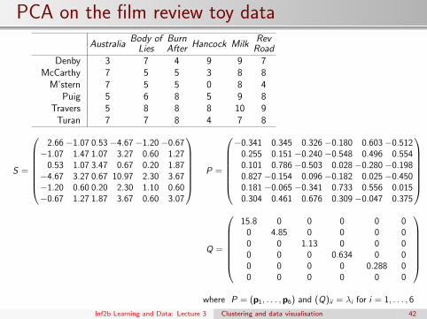
PCA on the film review toy dataBody of Burn Rev

Australia Lies After Hancock Milk RoadDenby 3 7 4 9 9 7

McCarthy 7 5 5 3 8 8M’stern 7 5 5 0 8 4

Puig 5 6 8 5 9 8Travers 5 8 8 8 10 9

Turan 7 7 8 4 7 8

S =

2.66 −1.07 0.53 −4.67 −1.20 −0.67−1.07 1.47 1.07 3.27 0.60 1.27

0.53 1.07 3.47 0.67 0.20 1.87−4.67 3.27 0.67 10.97 2.30 3.67−1.20 0.60 0.20 2.30 1.10 0.60−0.67 1.27 1.87 3.67 0.60 3.07

P =

−0.341 0.345 0.326 −0.180 0.603 −0.512

0.255 0.151 −0.240 −0.548 0.496 0.5540.101 0.786 −0.503 0.028 −0.280 −0.1980.827 −0.154 0.096 −0.182 0.025 −0.4500.181 −0.065 −0.341 0.733 0.556 0.0150.304 0.461 0.676 0.309 −0.047 0.375

Q =

15.8 0 0 0 0 0

0 4.85 0 0 0 00 0 1.13 0 0 00 0 0 0.634 0 00 0 0 0 0.288 00 0 0 0 0 0

where P = (p1, . . . ,p6) and (Q)ii = λi for i = 1, . . . , 6

Inf2b Learning and Data: Lecture 3 Clustering and data visualisation 42

PCA on the film review toy data (cont.)

6

7

8

9

10

11

12

13

2 4 6 8 10 12 14

2nd principal component

1st principal component

Denby

McCarthy

Morgenstern

PuigTravers

Turan

Inf2b Learning and Data: Lecture 3 Clustering and data visualisation 43

Dimensionality reduction D → ` by PCA

y1

y2...y`

=

pT

1 xpT

2 x...

pT` x

=

pT

1

pT2...

pT`

x

where {pi}`i=1 are the eigen vectors for the ` largest eigenvalues of S . The above can be rewritten as

y = ATx · · · linear transformation from RD to R`

y = (y1, . . . , y`)T : `-dimensional vector

A = (p1, . . . ,p`) : D × ` matrix

In many applications, we normalise data before PCA, e.g. y = AT (x− x).Inf2b Learning and Data: Lecture 3 Clustering and data visualisation 44

Summary

ClusteringK -means for minimising ‘cluster variance’Review notes, not just slides[other methods exist: hierarchical, top-down and bottom-up]

Unsupervised learningSpot structure in unlabelled dataCombine with knowledge of task

Principal Component Analysis (PCA)Find principal component axes for dimensionalityreduction and visualisation

Try implementing the algorithm! (Lab 3 this week)

Inf2b Learning and Data: Lecture 3 Clustering and data visualisation 45

Quizes

Q1: Find computational complexity of k-means algorithm

Q2: For k-means clustering, discuss possible methods formitigating the local minimum problem.

Q3: Discuss possible problems with k-means clustering andsolutions when the variances of data (i.e. si , i =1, . . . ,D)are much different from each other.

Q4: For k-means clustering, show E (t+1) ≤ E (t). (NE)

Q5: At page 37, show y = uTx.

Q6: At page 39, show Var (y) = λ1, where λ1 is the largesteigen value of S . (NE)

Q7: The first principal component axis is sometimes confusedwith the line of least squares fitting (or regression line).Explain the difference.

Inf2b Learning and Data: Lecture 3 Clustering and data visualisation 46