inf2b learning and data - lecture 5: introduction to statistical pattern
TRANSCRIPT

Inf2b Learning and DataLecture 5: Introduction to statistical pattern recognition
Hiroshi Shimodaira(Credit: Iain Murray and Steve Renals)
Centre for Speech Technology Research (CSTR)School of Informatics
University of Edinburgh
Jan-Mar 2014
Inf2b Learning and Data: Lecture 5 Introduction to statistical pattern recognition 1

Today’s Schedule
1 Probability (review)
2 What is Bayes’ theorem for?
3 Statistical classification
Inf2b Learning and Data: Lecture 5 Introduction to statistical pattern recognition 2

Motivation for probability
In some applications we need to:
Communicate uncertainty
Use prior knowledge
Deal with missing data
(we cannot easily measure similarity)
Inf2b Learning and Data: Lecture 5 Introduction to statistical pattern recognition 3
1 Probability (review)
2 What is Bayes’ theorem for?
3 Statistical classification
Inf2b Learning and Data: Lecture 5 Introduction to statistical pattern recognition 4
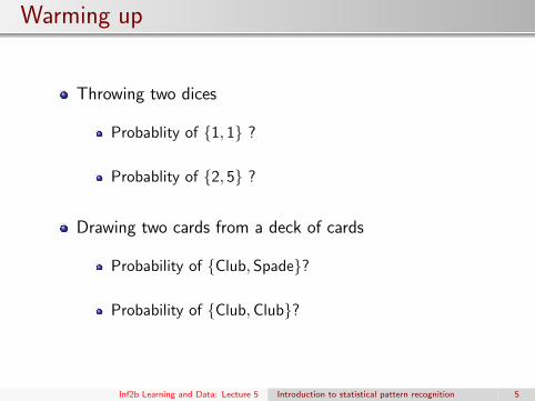
Warming up
Throwing two dices
Probablity of {1, 1} ?
1
6× 6=
1
36
Probablity of {2, 5} ?
2
6× 6=
1
18
Drawing two cards from a deck of cards
Probability of {Club,Spade}?
13× 13× 2
52× 51=
13
102
Probability of {Club,Club}?
13× 12
52× 51=
1
17
Inf2b Learning and Data: Lecture 5 Introduction to statistical pattern recognition 5
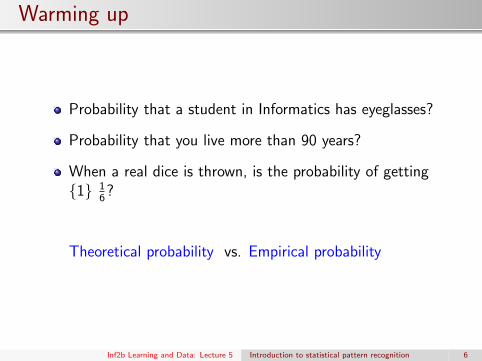
Warming up
Probability that a student in Informatics has eyeglasses?
Probability that you live more than 90 years?
When a real dice is thrown, is the probability of getting{1} 1
6?
Theoretical probability vs. Empirical probability
Inf2b Learning and Data: Lecture 5 Introduction to statistical pattern recognition 6

Rules of Probability
Sum Rule:
P(X =xi) =L∑
j=1
P(X =xi ,Y =yj)
Product Rule:
P(Y =yj ,X =xi) = P(Y =yj |X =xi)P(X =xi)
= P(X =xi |Y =yj)P(Y =yj)
Random variables Events/values
X {x1, x2, . . . , xL}Y {y1, y2, . . . , yL}
Inf2b Learning and Data: Lecture 5 Introduction to statistical pattern recognition 7
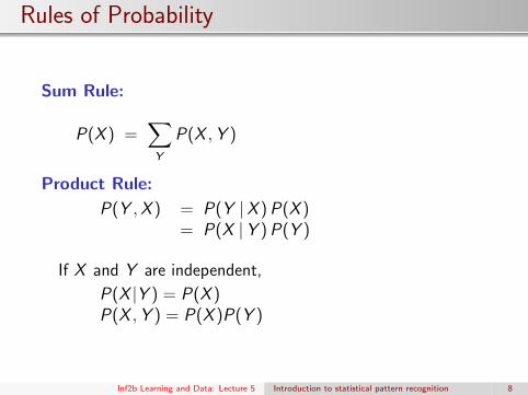
Rules of Probability
Sum Rule:
P(X ) =∑Y
P(X ,Y )
Product Rule:
P(Y ,X ) = P(Y |X )P(X )= P(X |Y )P(Y )
If X and Y are independent,
P(X |Y ) = P(X )P(X ,Y ) = P(X )P(Y )
Inf2b Learning and Data: Lecture 5 Introduction to statistical pattern recognition 8
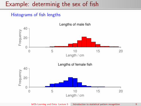
Example: determinig the sex of fish
Histograms of fish lengths
0 5 10 15 200
20
40
Fre
qu
en
cy
Length / cm
Lengths of male fish
0 5 10 15 200
20
40
Fre
qu
en
cy
Length / cm
Lengths of female fish
Inf2b Learning and Data: Lecture 5 Introduction to statistical pattern recognition 9

Example: determinig the sex of fish
Relative frequencies of fish length
0 5 10 15 200
0.2
0.4
Re
l. F
req
.
Length / cm
Lengths of male fish
0 5 10 15 200
0.2
0.4
Re
l. F
req
.
Length / cm
Lengths of female fish
Inf2b Learning and Data: Lecture 5 Introduction to statistical pattern recognition 10

Example: determinig the sex of fish
Possible decision boundary
0 5 10 15 200
0.2
0.4
Rel
.Fre
q.
Length / cm
Lengths of male fish
0 5 10 15 200
0.2
0.4
Rel
.Fre
q.
Length / cm
Lengths of female fish
Inf2b Learning and Data: Lecture 5 Introduction to statistical pattern recognition 11

Fish questions
How to classify 4 cm, or 19 cm fish?
How to classify 22 cm fish?
How to classify 10 cm fish?
What if there are 10× more male fish than female?
What if you’re forbidden from catching female fish?
0 5 10 15 200
0.2
0.4
Rel
.Fre
q.
Length / cm
Lengths of male fish
0 5 10 15 200
0.2
0.4
Rel
.Fre
q.
Length / cm
Lengths of female fish
Inf2b Learning and Data: Lecture 5 Introduction to statistical pattern recognition 12

Fish questions
Relative frequeny of male fish length: P(X = x |C = M)Relative frequeny of female fish length: P(X = x |C = F)
Given a fish length, x, is it sensible to decide as follows?
male fish if P(x |M) > P(x |F)female fish if P(x |M) < P(x |F)
0 5 10 15 200
0.2
0.4
Rel
.Fre
q.
Length / cm
Lengths of male fish
0 5 10 15 200
0.2
0.4
Rel
.Fre
q.
Length / cm
Lengths of female fish
Inf2b Learning and Data: Lecture 5 Introduction to statistical pattern recognition 13

Bayes’ Theorem
P(Y |X ) =P(X |Y )P(Y )
P(X )
Tohmas Bayes (?) (1701? – 1761)
http://www.york.ac.uk/depts/maths/histstat/bayespic.htm
Inf2b Learning and Data: Lecture 5 Introduction to statistical pattern recognition 14
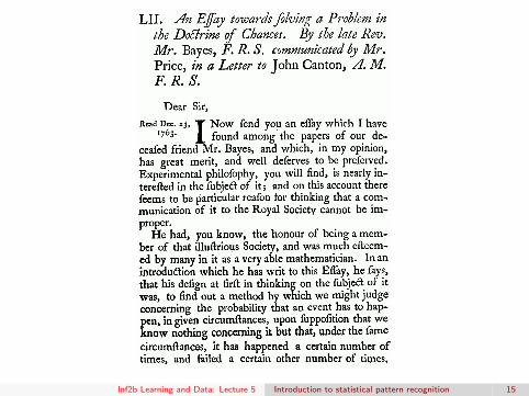
Inf2b Learning and Data: Lecture 5 Introduction to statistical pattern recognition 15
‘Bayesian’ philosophy refs
Non-examinable!
Bayes’ paper:http://www.jstor.org/stable/105741
http://dx.doi.org/10.1093/biomet/45.3-4.296 (re-typeset)
Cox’s paper:http://dx.doi.org/10.1119/1.1990764
http://dx.doi.org/10.1016/S0888-613X(03)00051-3 modern
commentary
MacKay textbook, amongst many others
Inf2b Learning and Data: Lecture 5 Introduction to statistical pattern recognition 16
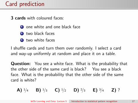
Card prediction
3 cards with coloured faces:
1 one white and one black face
2 two black faces
3 two white faces
I shuffle cards and turn them over randomly. I select a cardand way-up uniformly at random and place it on a table.
Question: You see a white face. What is the probability thatthe other side of the same card is black? You see a blackface. What is the probability that the other side of the samecard is white?
A) 1/4 B) 1/3 C) 1/2 D) 2/3 E) 3/4 Z) ?
Inf2b Learning and Data: Lecture 5 Introduction to statistical pattern recognition 17

Notes on the card prediction problem:
This card problem is Ex. 8.10a), MacKay, p142.It is not the same as the famous ‘Monty Hall’ puzzle: Ex. 3.8–9 andhttp://en.wikipedia.org/wiki/Monty_Hall_problem
The Monty Hall problem is also worth understanding. Although the cardproblem is (hopefully) less controversial and more straightforward. Theprocess by which a card is selected should be clear: P(c) = 1/3 forc = 1, 2, 3, and the face you see first is chosen at random: e.g.,P(x1 =B | c =1) = 0.5.Many people get this puzzle wrong on first viewing (it’s easy to messup). If you do get the answer right immediately (are you sure?), this iswill be a simple example on which to demonstrate some formalism.
Inf2b Learning and Data: Lecture 5 Introduction to statistical pattern recognition 18

How do we solve it formally?
Use Bayes theorem?
P(x2 =W | x1 =B) =P(x1 =B | x2 =W) P(x2 =W)
P(x1 =B)
The boxed term is no more obvious than the answer!
Bayes theorem is used to ‘invert’ forward generative processesthat we understand.The first step to solve inference problems is to write down amodel of your data.
Inf2b Learning and Data: Lecture 5 Introduction to statistical pattern recognition 19

The card game model
Cards: 1) B|W, 2) B|B, 3) W|W
P(c) =
{1/3 c = 1, 2, 3
0 otherwise.
P(x1 =B | c) =
1/2 c = 1
1 c = 2
0 c = 3
Bayes theorem can ‘invert’ this to tell us P(c | x1 =B);infer the generative process for the data we have.
Inf2b Learning and Data: Lecture 5 Introduction to statistical pattern recognition 20
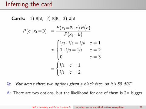
Inferring the card
Cards: 1) B|W, 2) B|B, 3) W|W
P(c | x1 =B) =P(x1 =B | c)P(c)
P(x1 =B)
∝
1/2 · 1/3 = 1/6 c = 1
1 · 1/3 = 1/3 c = 2
0 c = 3
=
{1/3 c = 12/3 c = 2
Q: “But aren’t there two options given a black face, so it’s 50–50?”
A: There are two options, but the likelihood for one of them is 2× bigger
Inf2b Learning and Data: Lecture 5 Introduction to statistical pattern recognition 21
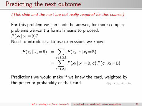
Predicting the next outcome
(This slide and the next are not really required for this course.)
For this problem we can spot the answer, for more complexproblems we want a formal means to proceed.P(x2 | x1 =B)?Need to introduce c to use expressions we know:
P(x2 | x1 =B) =∑
c∈1,2,3
P(x2, c | x1 =B)
=∑
c∈1,2,3
P(x2 | x1 =B, c)P(c | x1 =B)
Predictions we would make if we knew the card, weighted bythe posterior probability of that card. P(x2=W | x1=B) = 1/3
Inf2b Learning and Data: Lecture 5 Introduction to statistical pattern recognition 22

Strategy for solving any inference and prediction problem:
When interested in something y , we often find we can’timmediately write down mathematical expressions for P(y | data).So we introduce stuff, z , that helps us define the problem:
P(y | data) =∑z
P(y , z | data)
by using the sum rule. And then split it up:
P(y | data) =∑z
P(y | z , data)P(z | data)
using the product rule. If knowing extra stuff z we can predict y ,we are set: weight all such predictions by the posterior probabilityof the stuff (P(z | data), found with Bayes theorem).Sometimes the extra stuff summarizes everything we need to knowto make a prediction:
P(y | z , data) = P(y | z)
although not in the formulation of the card game above.Inf2b Learning and Data: Lecture 5 Introduction to statistical pattern recognition 23

Not convinced?
Not everyone believes the answer to the card game question.Sometimes probabilities are counter-intuitive. I’d encourage you to writesimulations of these games if you are at all uncertain. Here is anOctave/Matlab simulator I wrote for the card game question:cards = [1 1;
0 0;
1 0];
num cards = size(cards, 1);
N = 0; % Number of times first face is black
kk = 0; % Out of those, how many times the other side is white
for trial = 1:1e6
card = ceil(num cards * rand());
face = 1 + (rand < 0.5);
other face = (face==1) + 1;
x1 = cards(card, face);
x2 = cards(card, other face);
if x1 == 0
N = N + 1;
kk = kk + (x2 == 1);
end
end
approx probability = kk / N
Inf2b Learning and Data: Lecture 5 Introduction to statistical pattern recognition 24

1 Probability (review)
2 What is Bayes’ theorem for?
3 Statistical classification
Inf2b Learning and Data: Lecture 5 Introduction to statistical pattern recognition 25
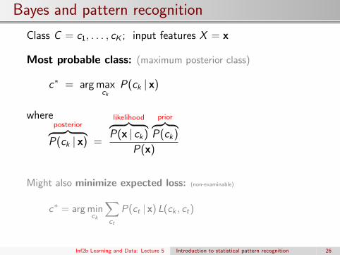
Bayes and pattern recognition
Class C = c1, . . . , cK ; input features X = x
Most probable class: (maximum posterior class)
c∗ = arg maxck
P(ck | x)
whereposterior︷ ︸︸ ︷P(ck | x) =
likelihood︷ ︸︸ ︷P(x | ck)
prior︷ ︸︸ ︷P(ck)
P(x)
Might also minimize expected loss: (non-examinable)
c∗ = arg minck
∑ct
P(ct | x) L(ck , ct)
Inf2b Learning and Data: Lecture 5 Introduction to statistical pattern recognition 26

Posterior probability
Can compute denominator with sum rule:
P(x) =∑`
P(x | c`)P(c`)
However P(x) is the same for all classes:
P(ck | x) ∝ P(x | ck)P(ck)
Choosing between two classes, only requires the odds,the ratio of the posterior probabilities.
Inf2b Learning and Data: Lecture 5 Introduction to statistical pattern recognition 27
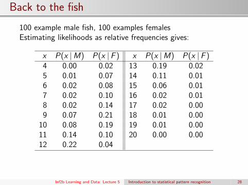
Back to the fish
100 example male fish, 100 examples femalesEstimating likelihoods as relative frequencies gives:
x P(x |M) P(x |F ) x P(x |M) P(x |F )4 0.00 0.02 13 0.19 0.025 0.01 0.07 14 0.11 0.016 0.02 0.08 15 0.06 0.017 0.02 0.10 16 0.02 0.018 0.02 0.14 17 0.02 0.009 0.07 0.21 18 0.01 0.00
10 0.08 0.19 19 0.01 0.0011 0.14 0.10 20 0.00 0.0012 0.22 0.04
Inf2b Learning and Data: Lecture 5 Introduction to statistical pattern recognition 28
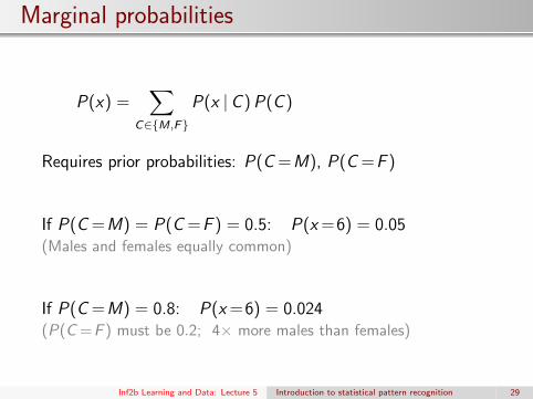
Marginal probabilities
P(x) =∑
C∈{M,F}
P(x |C )P(C )
Requires prior probabilities: P(C =M), P(C =F )
If P(C =M) = P(C =F ) = 0.5: P(x =6) = 0.05(Males and females equally common)
If P(C =M) = 0.8: P(x =6) = 0.024(P(C =F ) must be 0.2; 4× more males than females)
Inf2b Learning and Data: Lecture 5 Introduction to statistical pattern recognition 29

Inferring labels for x =11
Equal prior probabilities: classify it as male:
P(M | x)
P(F | x)=
P(x |M)P(M)
P(x |F )P(F )=
0.14 · 0.50.10 · 0.5
= 1.4
Twice as many females as males: (i.e., P(M) = 1/3, P(F ) = 2/3)
P(M | x)
P(F | x)=
P(x |M)P(M)
P(x |F )P(F )=
0.14 · 1/3
0.10 · 2/3= 0.7
Classify it as femaleM:F is 0.7:1, that is, P(M | x) = 0.7/(0.7 + 1) ≈ 0.41
Inf2b Learning and Data: Lecture 5 Introduction to statistical pattern recognition 30
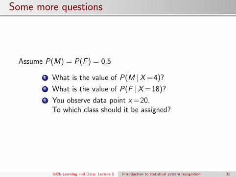
Some more questions
Assume P(M) = P(F ) = 0.5
1 What is the value of P(M |X =4)?
2 What is the value of P(F |X =18)?
3 You observe data point x =20.To which class should it be assigned?
Inf2b Learning and Data: Lecture 5 Introduction to statistical pattern recognition 31

Work through the notes!
Remember to review the notes. . .. . . work through the fruit box example
Similar material in this online text:http://www.greenteapress.com/thinkbayes/html/thinkbayes002.html
Inf2b Learning and Data: Lecture 5 Introduction to statistical pattern recognition 32