inference for multi- n i l dimensional r high-frequency
TRANSCRIPT
SFB 649 Discussion Paper 2013-006
Inference for Multi-Dimensional
High-Frequency Data: Equivalence of
Methods, Central Limit Theorems, and an
Application to Conditional
Independence Testing
Markus Bibinger* Per A. Mykland**
* Humboldt-Universität zu Berlin, Germany
** University of Chicago, U.S.A.
This research was supported by the Deutsche Forschungsgemeinschaft through the SFB 649 "Economic Risk".
http://sfb649.wiwi.hu-berlin.de
ISSN 1860-5664
SFB 649, Humboldt-Universität zu Berlin Spandauer Straße 1, D-10178 Berlin
SFB
6
4 9
E
C O
N O
M I
C
R
I S
K
B
E R
L I
N
Inference for Multi-DimensionalHigh-Frequency Data: Equivalence of Methods,Central Limit Theorems, and an Application to
Conditional Independence TestingMarkus Bibinger & Per A. Mykland
Humboldt-Universitat zu Berlin and Department of Statistics, University of Chicago
ABSTRACT. We find the asymptotic distribution of the multi-dimensional multi-scale and kernelestimators for high-frequency financial data with microstructure. Sampling times are allowed tobe asynchronous. The central limit theorem is shown to have a feasible version. In the process,we show that the classes of multi-scale and kernel estimators for smoothing noise perturbation areasymptotically equivalent in the sense of having the same asymptotic distribution for correspondingkernel and weight functions. We also include the analysis for the Hayashi-Yoshida estimator inabsence of microstructure.The theory leads to multi-dimensional stable central limit theorems for respective estimators andhence allows to draw statistical inference for a broad class of multivariate models and linear functionsof the recorded components. This paves the way to tests and confidence intervals in risk measurementfor arbitrary portfolios composed of high-frequently observed assets. As an application, we enhancethe approach to cover more complex functions and in order to construct a test for investigatinghypotheses that correlated assets are independent conditional on a common factor.
Key words: asymptotic distribution theory, asynchronous observations, conditional independence, high-frequency data,microstructure noise, multivariate limit theorems
JEL Classification: C14, C32, C58, G10
1 IntroductionThe estimation of daily integrated variance and covariance1 has become a central building block in modelcalibration for financial risk analysis. Recent years have seen a tremendous increase in trading activitiesalong with ongoing buildup of computer-based trading. The availability of recorded asset prices at suchhigh frequencies magnifies the appeal of asset price models grounded on continuous-time stochastic pro-cesses which are a cornerstone of financial modeling since the seminal works by Black & Scholes (1973)and Heston (1993). Increasing observation frequencies makes it possible to consider efficient estimationfrom underlying statistical experiments. Rising demand for an advanced theoretical foundation thus gavebirth to the field of statistics for high-frequency data, going back to the path-breaking work of Andersen &Bollerslev (1998), Andersen et al. (2001, 2003), and Barndorff-Nielsen & Shephard (2001, 2002).This article contributes to this strand of literature by considering a continuous-time stochastic process,i. e. a continuous semimartingale X comprising current stochastic volatility models, observed on a fixedtime span [0, T ] at (n + 1) points of a discrete grid and by investigating asymptotics when the mesh sizeof the grid tends to zero. A natural estimator for the integrated variance of a process is the discrete versioncalled realized variance or realized volatility. For a continuous semimartingale, this estimator is consis-tent, and it weakly converges with usual
√n-rate to a mixed normal distribution where twice the integrated
quarticity occurs as random asymptotic variance (Barndorff-Nielsen & Shephard (2002), Jacod & Prot-ter (1998), Zhang (2001)). Therefore, the concept of stable weak convergence by Renyi (1963) has beencalled into play to pave the way for statistical inference and confidence intervals. In our setting, stable
1More accurately known as integrated volatilities and covolatilities, but we here stick to the more heavily used terminology.
1
convergence is equivalent to joint weak convergence with every measurable bounded random variable2
and thus, accompanied by a consistent estimator of the asymptotic variance, allows to conclude a feasiblecentral limit theorem. This reasoning makes stable convergence a key element in high-frequency asymp-totic statistics, and it completes the asymptotic distribution theory for a univariate setup.3 Yet, an apparentproblem pertinent to applications is to quantify the risk of a collection of high-frequently observed assets.Suppose we wish to estimate the quadratic variation of a sum X1 + X2, both processes X1 and X2 docu-mented as high-frequency data and modeled by continuous semimartingales. The quadratic variation of thesum is the sum of integrated variances and twice the integrated covariance. For the latter, the derivation of afeasible central limit theorem is evident as for its one-dimensional counterpart. However, when estimating[X1 + X2] with the sum of these estimates, we do not obtain a feasible asymptotic distribution theory forthis combined estimator for free. This is due to the fact, that the single estimates are correlated. To deducethe asymptotic variance of the compound estimator, we are in need of a multivariate limit theorem involv-ing the asymptotic covariance matrix of the estimators. The first part of this article is devoted to that taskand provides asymptotic covariances of covariance matrix estimators within prominent specific models forhigh-frequency data.The aspiration to progress to more complex statistical models in this research area, has again been mainlymotivated by economic issues. First of all, in a multi-dimensional framework, different assets are usuallynot traded and recorded at synchronous sampling times, but geared to individual observation schemes.Employing simple interpolation approaches has led to the so-called Epps effect (cf. Epps (1979)) that co-variance estimates get heavily biased downwards at high frequencies by the distortion from an inadequatetreatment of non-synchronicity. In the absence of microstructure, the estimator by Hayashi & Yoshida(2005) remedies this flaw of naively interpolated realized covariances and a feasible central limit theoremhas been attained in Hayashi & Yoshida (2011).For one-dimensional high-frequency data, increasing sample sizes are expected to render the estimationerror by discretization smaller and smaller – which is clearly the case if we assume an underlain contin-uous semimartingale. Contrary to the feature of the statistical model, in many situations high-frequencyfinancial data exhibit an exploding realized variance when the sampling frequency is too high.4 This ef-fect is ascribed to market microstructure frictions as bid-ask spreads and trading costs. A favored wayto capture this influence is to extend the classical semimartingale model, where the semimartingale actsto describe dynamics of the evolution of a latent efficient log-price which is corrupted by an independentadditive noise. Following this philosophy from Zhang et al. (2005), several integrated variance estima-tors have been designed which smooth out noise contamination first. The optimal minimax convergencerate for this model declines to n1/4, what is known from the mathematical groundwork provided by Gloter& Jacod (2001). This rate can be attained using the multi-scale realized variance by Zhang (2006), pre-averaging as described in Jacod et al. (2009), the kernel estimator by Barndorff-Nielsen et al. (2008) or aQuasi-Maximum-Likelihood approach by Xiu (2010). Though the estimators have been found in indepen-dent works and rely on various principles, it turned out that they are actually quite similar and in a certainasymptotic sense equivalent which is clarified in Section 3 below.The approaches to cope with microstructure noise analogously carry over to the synchronous multi-dimen-sional setting. Recently, methods to deal with noise and non-synchronicity in one go have been estab-lished in the literature. In fact, to each of the abovementioned smoothing techniques one extension to non-synchronous observation schemes has been proposed. First, the multivariate realised kernels by Barndorff-Nielsen et al. (2011) using refresh time sampling are eligible to estimate integrated covariance matrices andguarantee for positive semi-definite estimates at the cost of a sub-optimal convergence rate. Aıt-Sahaliaet al. (2010) suggested to combine a generalized synchronization algorithm with the Quasi-Maximum-Likelihood approach. Eventually, a feasible asymptotic distribution theory for the general non-synchronousand noisy setup has been provided by Bibinger (2012) and Christensen et al. (2011) for hybrid approachesbuilt on the Hayashi–Yoshida estimator and the multi-scale and pre-average smoothing, respectively. Al-though these estimators combine similar ingredients they behave quite differently, since for the approachin Bibinger (2012) interpolation takes place on the high-frequency scale after smoothing is adjusted with
2For a discussion of the general case, see p. 270 of Jacod & Protter (1998).3See Section 2 for definition and further discussion.4This is usually seen with the help of a so-called signature plot, see Andersen et al. (2000) and also the discussion in Chapter 2.5.2
of Mykland & Zhang (2012).
2
respect to a synchronous approximation whereas Christensen et al. (2011) suggest to denoise each processfirst and take the Hayashi-Yoshida estimator from pre-averaged blocks which results in interpolation withrespect to a lower-frequency scale. Park & Linton (2012) use Fourier methods on the same problem.
Remarkably, when interpolations in the fashion of the Hayashi-Yoshida estimator are performed onthe high-frequency scale their impact on the asymptotic discretization variance of the hybrid generalizedmulti-scale estimator vanishes asymptotically at the slower convergence rate in the presence of noise.5 Thisreveals that non-synchronicity becomes less important in the latent observation model with noise dilution.In all four models, discretely observed continuous semimartingales with or without noise, synchronously ornon-synchronously, we develop the asymptotic covariance structure of the respective estimation methods.We choose the realized covariance matrix, the multi-scale, the Hayashi-Yoshida and the generalized multi-scale estimator to establish the multivariate limit theorems. While the asymptotic covariances for the syn-chronous settings are found following a similar strategy as for the asymptotic variances, the most intricatechallenge arises for non-synchronous sampling schemes. The asymptotic variance of the Hayashi-Yoshidaestimator can be illuminated as in Bibinger (2011a) by a synchronous approximation and interpolationsand hinges on an interplay of the two different sampling grids. For covariances, we consider two Hayashi-Yoshida estimates with generally four different sampling schemes. Nevertheless, utilizing an illustrationwith refresh times of pairs and quadruplets will reveal the nature of the asymptotic covariance. For thegeneralized multi-scale estimator in the most general setup we benefit again from the fact that interpolationeffects fall out asymptotically. Yet, the effects by superposition with noise require a tedious notation tocover all possible sampling designs. In typical situations, as a completely asynchronous sampling design,only the signal parts will contribute to asymptotic covariances, and the multivariate distribution simplifiesleading to a tractable general approach.Relying on the asymptotic distribution of the considered integrated covariance matrix estimators, we striveto design a statistical test for investigating hypotheses, if two processes have zero covariation conditionedon a third one. We end up with a feasible stable central limit theorem for the test statistic involving productsof estimators and thus obtain an asymptotic distribution free test. This test which we call conveniently con-ditional independence test renders information about the dependence structure in multivariate portfoliosand can be applied to test for zero covariation of idiosyncratic factors in typical portfolio dependence struc-ture models, as the one by Eberlein et al. (2008). In particular, we may identify dependencies betweensingle assets not carried in common macroeconomic factors that influence the whole portfolio and disen-tangle those from correlations induced by market influences.The outline of the article is as follows. We start in Section 2 by discussing asymptotic covariance matricesfor the realized covariances in a simple equidistant discretely observed Ito process setup. We proceed tostatistical experiments with noise in Section 3, non-synchronous sampling in Section 4 and both at thesame time in Section 5. In Section 6, the results are gathered to conclude feasible multivariate central limittheorems. The conditional independence test is introduced in Section 7 and after an empirical study ofasymptotic covariances applied in Section 8 to high-frequency financial data. The proofs can be found inAppendix A.
2 The simple case: Asymptotic covariance matrix of realized covari-ances
Assumption 1. Consider a continuous p-dimensional Ito semimartingale (Ito process)
Xt = X0 +
∫ t
0
µs ds+
∫ t
0
σs dWs , t ∈ R+ , (1)
adapted with respect to a right-continuous and complete filtration (Ft) on a filtered probability space(Ω,F , (Ft),P) with adapted locally bounded drift process µ, a p-dimensional Brownian motion W andadapted p × p′ cadlag volatility process σ. Suppose that σ itself is an Ito process again, given by anequation similar to (1). The processes σ and W can be dependent, allowing for leverage effect.
5 Similar findings were made for the two-scales estimator in Zhang (2011), and for local likelihood in Bibinger et al. (2012).
3
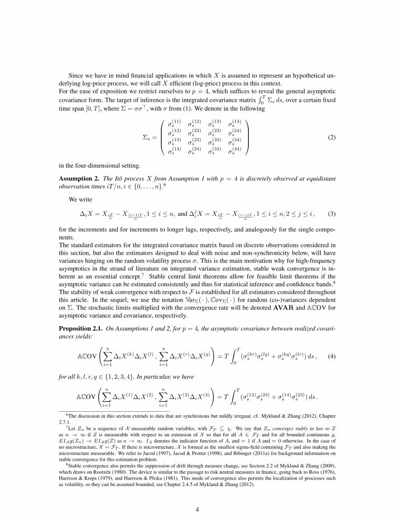
Since we have in mind financial applications in which X is assumed to represent an hypothetical un-derlying log-price process, we will call X efficient (log-price) process in this context.For the ease of exposition we restrict ourselves to p = 4, which suffices to reveal the general asymptoticcovariance form. The target of inference is the integrated covariance matrix
∫ T0
Σs ds, over a certain fixedtime span [0, T ], where Σ = σσ>, with σ from (1). We denote in the following
Σs =
σ
(11)s σ
(12)s σ
(13)s σ
(14)s
σ(12)s σ
(22)s σ
(23)s σ
(24)s
σ(13)s σ
(23)s σ
(33)s σ
(34)s
σ(14)s σ
(24)s σ
(34)s σ
(44)s
(2)
in the four-dimensional setting.
Assumption 2. The Ito process X from Assumption 1 with p = 4 is discretely observed at equidistantobservation times iT/n, i ∈ 0, . . . , n.6
We write
∆iX = X iTn−X (i−1)T
n, 1 ≤ i ≤ n, and ∆j
iX = X iTn−X (i−j)T
n, 1 ≤ i ≤ n, 2 ≤ j ≤ i , (3)
for the increments and for increments to longer lags, respectively, and analogously for the single compo-nents.The standard estimators for the integrated covariance matrix based on discrete observations considered inthis section, but also the estimators designed to deal with noise and non-synchronicity below, will havevariances hinging on the random volatility process σ. This is the main motivation why for high-frequencyasymptotics in the strand of literature on integrated variance estimation, stable weak convergence is in-herent as an essential concept.7 Stable central limit theorems allow for feasible limit theorems if theasymptotic variance can be estimated consistently and thus for statistical inference and confidence bands.8
The stability of weak convergence with respect to F is established for all estimators considered throughoutthis article. In the sequel, we use the notation VarΣ( · ),CovΣ( · ) for random (co-)variances dependenton Σ. The stochastic limits multiplied with the convergence rate will be denoted AVAR and ACOV forasymptotic variance and covariance, respectively.
Proposition 2.1. On Assumptions 1 and 2, for p = 4, the asymptotic covariance between realized covari-ances yields:
ACOV
(n∑i=1
∆iX(k)∆iX
(l) ,n∑i=1
∆iX(r)∆iX
(q)
)= T
∫ T
0
(σ(kr)s σ(lq)
s + σ(kq)s σ(lr)
s ) ds , (4)
for all k, l, r, q ∈ 1, 2, 3, 4. In particular, we have
ACOV
(n∑i=1
∆iX(1)∆iX
(2) ,
n∑i=1
∆iX(3)∆iX
(4)
)= T
∫ T
0
(σ(13)s σ(24)
s + σ(14)s σ(23)
s ) ds .
6The discussion in this section extends to data that are synchronous but mildly irreguar, cf. Mykland & Zhang (2012), Chapter2.7.1.
7Let Zn be a sequence of X -measurable random variables, with FT ⊆ χ. We say that Zn converges stably in law to Zas n → ∞ if Z is measurable with respect to an extension of X so that for all A ∈ FT and for all bounded continuous g,EIAg(Zn) → EIAg(Z) as n → ∞. IA denotes the indicator function of A, and = 1 if A and = 0 otherwise. In the case ofno microstructure, X = FT . If there is microstructure, X is formed as the smallest sigma-field containing FT and also making themicrostructure measurable. We refer to Jacod (1997), Jacod & Protter (1998), and Bibinger (2011a) for background information onstable convergence for this estimation problem.
8Stable convergence also permits the suppression of drift through measure change, see Section 2.2 of Mykland & Zhang (2009),which draws on Rootzen (1980). The device is similar to the passage to risk neutral measures in finance, going back to Ross (1976),Harrison & Kreps (1979), and Harrison & Pliska (1981). This mode of convergence also permits the localization of processes suchas volatility, so they can be assumed bounded, see Chapter 2.4.5 of Mykland & Zhang (2012).
4
A generalization for non-equidistant sampling is covered by Proposition 4.1 in Section 4. From nowon we express the general asymptotic covariances using indices 1, 2, 3, 4 as in the second formula above,and obtain special cases by inserting ‘(1) = (2)’ etc. Proposition 2.1 includes the well-known results that
nVarΣ
(n∑i=1
(∆iX)2
)p−→ 2T
∫ T
0
σ4s ds
for the realized variance in a one-dimensional setup, where the asymptotic variance hinges on the so-calledintegrated quarticity, and
nVarΣ
(n∑i=1
∆iX(1)∆iX
(2)
)p−→ T
∫ T
0
(1 + ρ2s)(σ
(1)s σ(2)
s )2 ds
in a bivariate model with spot correlation process ρs. Already in the two-dimensional model we addition-ally obtain asymptotic covariances between realized variances and the realized covariance
nCovΣ
(n∑i=1
∆iX(1)∆iX
(2) ,
n∑i=1
(∆iX(1))2
)p−→ 2T
∫ T
0
ρs(σ(1)s )3σ(2)
s ds .
The key steps for proving (4) are the approximation
∆iX ≈ σ (i−1)Tn
(W iT
n−W (i−1)T
n
), (5)
more precisely given in the Appendix A, and the formula
Cov(Z(i)Z(l), Z(m)Z(u)
)= ΣimΣlu + ΣiuΣlm . (6)
for a multivariate normal Z ∼ N(0,Σ) with covariance matrix (Σij). The right-hand side of (5) is condi-tionally on F(i−1)T/n centered Gaussian and this finding will be helpful, since by the martingale structureof realized (co-)variances and estimation errors in the upcoming sections below, the asymptotic covariancesare given as limit of the sequence of conditional covariances. Hence it will be possible to apply (6) whichis a special case of the general formula for moments from a multivariate normal by Isserlis (1918).
3 Inference for observations with microstructure noiseAssumption* 2. The process X is observed synchronously on [0, T ] with additive microstructure noise:
Yi = Xti + εi , i = 0, . . . , n .
The ti, 0 ≤ i ≤ n, are the observation times and we assume that there is a constant 0 < α ≤ 1/9, suchthat
δn = supi
((ti − ti−1) , t0, T − tn) = O(n−
8/9−α), (7)
stating that we allow for a maximum time instant tending to zero slower than with n−1, but not too slow.The microstructure noise is given as a discrete-time process for which the observation errors are assumedto be i. i. d. and independent of the efficient process. Furthermore, the errors have mean zero, and fourthmoments exist.
Exact orders in (7) and below in (18) and (25) arise from upper bounds of remainder terms after apply-ing Holder inequality. We keep to the notation
∆iX = Xti −Xti−1 and ∆jiX = Xti −Xti−j , 1 ≤ i ≤ n, 2 ≤ j ≤ i .
Since notation varies between papers, note the correspondence to the other main form:
∆iX is the same as ∆Xti .
5
The covariance matrix of the vectors εj , 0 ≤ j ≤ n, is denoted H and for p = 4 we set
H =
η1
2 η12 η13 η14
η12 η22 η23 η24
η13 η23 η32 η34
η14 η24 η34 η42
. (8)
Note that an i. i. d. assumption on the noise is standard in related literature, an extension to m-dependenceand mixing errors can be attained as in Aıt-Sahalia et al. (2011). For notational convenience of asymptoticvariances, we restrict ourselves to i. i. d. noise in this section – in the general asynchronous frameworkbelow asymptotic covariances of generalized multi-scale estimates are not affected by the noise.Increments in such a microstructure noise model
∆jY =
∫ tj
tj−1
µs ds+
∫ tj
tj−1
σs dWs + εj − εj−1
are substantially governed by the noise, since the second addend is Op(δ1/2n ) and the drift acts only as
nuisance term of order in probabilityOp(δn). For an accurate estimation of the integrated covariance matrixin the presence of noise smoothing methods are applied. We now discuss several main approaches andintegrate them in a unifying theory. To this end, we show that two prominent methods are asymptoticallyequivalent.
3.1 Asymptotic Equivalence of the Multi-Scale and Kernel EstimatorsFor the estimation of integrated variance the following rate-optimal estimators with similar asymptoticbehavior have been proposed in the literature: a multi-scale approach by Zhang (2006), pre-averaging noisyreturns first as in Jacod et al. (2009), the kernel approach by Barndorff-Nielsen et al. (2008) and a Quasi-Maximum-Likelihood-Estimator by Xiu (2010). We investigate the covariance structure of the multi-scaleestimator explicitly, but since all these estimators have a similar structure as quadratic form of the discreteobservations, analogous reasoning will apply to the other methods. In particular, we shed light on theconnection to the kernel approach to profit at the same time from the considerations by Barndorff-Nielsenet al. (2008) pertaining parametric efficiency and the asymptotic features of different kernel functions. Themulti-scale estimator
[X(1), X(2)
](multi)T
=
M(12)n∑i=1
αii
n∑j=i
∆ijY
(1)∆ijY
(2) , (9)
and analogous for other components, arises as linear combination of subsampling estimators that are aver-aged lower-frequent realized covariances using frequencies i = 1, . . . ,M
(12)n .
For discrete weights αi, 1 ≤ i ≤Mn, with∑Mn
i=1 αi = 1 and∑Mn
i=1(αi/i) = 0, the expression
αi =i
M2n
h
(i
Mn
)− i
2M3n
h′(
i
Mn
)+
i
6M4n
(h′(1)− h′(0))− i
24M5n
(h′′(1)− h′′(0)) , (10)
adopted from Zhang (2006), with twice continuously differentiable functions h satisfying∫ 1
0xh(x) dx = 1
and∫ 1
0h(x) dx = 0, gives access to a tractable class of estimators. The multi-scale frequencies are chosen
M(kl)n = ckl
√n with constants ckl, (k, l) ∈ 1, 2, 3, 42, minimizing the overall mean square error to order
n−1/4. The estimator is thus rate-optimal according to the lower bounds for convergence rates by Gloter &Jacod (2001) and Bibinger (2011b).At the present day, it is commonly known that the nonparametric smoothing approaches to cope with noisecontamination have a connatural structure and related asymptotic distribution. A prominent intensively
6
studied alternative to the multi-scale approach is the kernel estimator by Barndorff-Nielsen et al. (2008)
[X(1), X(2)
](kernel)T
=
n∑j=1
∆jY(1)∆jY
(2)
+
Hn∑h=1
K
(h
Hn
)( n∑j=h+1
∆jY(1)∆j−hY
(2) + ∆j−hY(1)∆jY
(2)), (11)
with a four times continuously differentiable kernel K on [0, 1], which satisfies the following conditions:
max
∫ 1
0
K2(x) dx,
∫ 1
0
(K′(x))2 dx,
∫ 1
0
(K′′(x))2 dx
<∞,K(0) = 1,K(1) = K′(0) = K′(1) = 0.
In the one-dimensional setup (11) has the shape of a linear combination of realized autocovariances ofthe discretely observed process. The subsequent explicit relation between kernel and multi-scale estimatorenables us to embed the findings about several kernels and the construction of an asymptotically efficientone for the scalar model provided by Barndorff-Nielsen et al. (2008). Since the multi-scale approachexhibits good finite-sample properties in the treatment of end-effects, it can be worth to road-test resultingtransferred multi-scale estimators in practice.
Theorem 3.1. For each kernel function K matching the assertions above, for the estimator defined in (11)and the multi-scale estimator (9) with weights determined by (10) and h = K′′, we have
n1/4
([
X(1), X(2)](multi)T
− [X(1), X(2)
](kernel)T
+ 4η12
)p−→ 0 , (12)
as n → ∞, Mn = Hn → ∞. The term 4η12 is due to the different impact of end-effects in (11) and (9)and, since the variance-covariance structure carries over to adjusted unbiased versions of the estimators,is not crucial for the relation of the asymptotic (co)variances.
3.2 Asymptotic Equivalence of Adjusted EstimatorsThe multi-scale and kernel estimators defined in (9) and (11) are sensitive to end-effects which is causedby the dominating noise component (which does not depend on n). Due to end-effects, on Assumption *2,the estimators (9) and (11) with weights determined by (10) and corresponding kernels have a bias −2η12
and 2η12, respectively. We here investigate a correction to each of the two types of estimator:Correction to Multi-scale: Follow Zhang (2006) by modifying the first two weights
α1 7→ α1 + 2/n, α2 7→ α2 − 2/n, (αi)3≤i≤Mn7→ (αi)3≤i≤Mn
. (13)
Correction to the Kernel estimator:
multiplying the realized covariance in the first addend withn− 1
n. (14)
This correction is different from the ‘jittering’ approach provided in Barndorff-Nielsen et al. (2008).9
We call the adjusted estimators, respectively,
[X(1), X(2)
](multi,adj)T
and [X(1), X(2)
](kernel,adj)T
.
With these adjustments, we obtain the following direct equivalence of the two estimators.
Theorem 3.2. Under the assumptions of Theorem 3.1, for each kernel function K, we have
n1/4
([
X(1), X(2)](multi,adj)T
− [X(1), X(2)
](kernel,adj)T
)p−→ 0 , (15)
as n→∞, Mn = cmulti√n and Hn = ckern
√n.
9Section 2.6 p. 1487-88 of Barndorff-Nielsen et al. (2008).
7
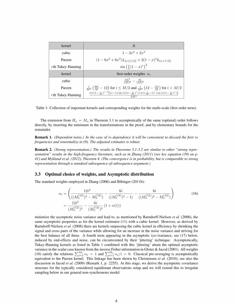
kernel K
cubic 1− 3x2 + 2x3
Parzen (1− 6x2 + 6x3)1x≤1/2 + 2(1− x)31x>1/2
rth Tukey-Hanning sin(π2 (1− x)r
)2kernel first-order weights αi
cubic 12i2
(M)3 −6i
(M)2
Parzen iM2
(36iM − 12
)for i ≤M/2 and i
M2
(12− 12i
M
)for i > M/2
rth Tukey-Hanningπir(1− i
M )r−2((r−1) sin (π(1− iM )r)+πr( i
M−1)r cos (π(1− iM )r))
2M2
Table 1: Collection of important kernels and corresponding weights for the multi-scale (first order term).
The extension from Hn = Mn in Theorem 3.1 to asymptotically of the same (optimal) order followsdirectly, by inserting the minimum in the transformations in the proof, and by elementary bounds for theremainder.
Remark 1. (Dependent noise.) In the case of m-dependence it will be convenient to discard the first mfrequencies and renormalize in (9). The adjusted estimator is robust.
Remark 2. (Strong representation.) The results in Theorems 3.1-3.2 are similar to other “strong repre-sentation” results in the high-frequency literature, such as in Zhang (2011) (see key equation (39) on p.41) and Mykland et al. (2012), Theorem 4. (The convergence is in probability, but is comparable to strongrepresentation through a standard subsequence-of-subsequence argument.)
3.3 Optimal choice of weights, and Asymptotic distributionThe standard weights employed in Zhang (2006) and Bibinger (2011b):
αi =
(12i2
((M(12)n )3 −M (12)
n )− 6i
((M(12)n )2 − 1)
− 6i
((M(12)n )3 −M (12)
n )
)(16)
=12i2
(M(12)n )3
− 6i
(M(12)n )2
(1 + O(1))
minimize the asymptotic noise variance and lead to, as mentioned by Barndorff-Nielsen et al. (2008), thesame asymptotic properties as for the kernel estimator (11) with a cubic kernel. However, as derived byBarndorff-Nielsen et al. (2008) there are kernels surpassing the cubic kernel in efficiency by shrinking thesignal and cross parts of the variance while allowing for an increase in the noise variance and striving forthe best balance of all three. A fourth term appearing in the asymptotic (co-)variance, see (17) below,induced by end-effects and noise, can be circumvented by their ‘jittering’ technique. Asymptotically,Tukey-Hanning kernels as listed in Table 1 combined with this ‘jittering’ attain the optimal asymptoticvariance in the scalar case known from the inverse Fisher information in Gloter & Jacod (2001). All weights(10) satisfy the relations
∑Mn
i=1 αi = 1 and∑Mn
i=1 αi/i = 0. Classical pre-averaging is asymptoticallyequivalent to the Parzen kernel. This linkage has been shown by Christensen et al. (2010); see also thediscussion in Jacod et al. (2009) (Remark 1, p. 2255). At this stage, we derive the asymptotic covariancestructure for the typically considered equidistant observations setup and we will extend this to irregularsampling below in our general non-synchronous model.
8
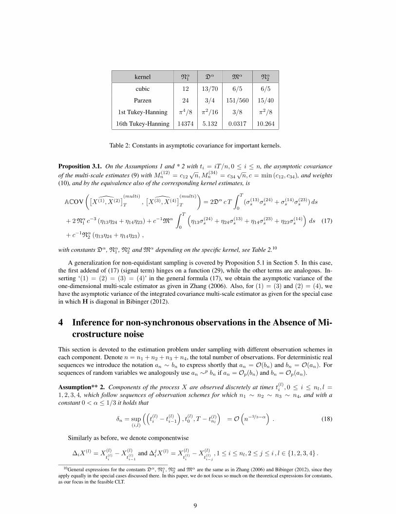
kernel Nα1 Dα Mα Nα
2
cubic 12 13/70 6/5 6/5
Parzen 24 3/4 151/560 15/40
1st Tukey-Hanning π4/8 π2/16 3/8 π2/8
16th Tukey-Hanning 14374 5.132 0.0317 10.264
Table 2: Constants in asymptotic covariance for important kernels.
Proposition 3.1. On the Assumptions 1 and * 2 with ti = iT/n, 0 ≤ i ≤ n, the asymptotic covarianceof the multi-scale estimates (9) with M (12)
n = c12√n,M
(34)n = c34
√n, c = min (c12, c34), and weights
(10), and by the equivalence also of the corresponding kernel estimates, is
ACOV(
[X(1), X(2)
](multi)T
, [X(3), X(4)
](multi)T
)= 2Dα c T
∫ T
0
(σ(13)s σ(24)
s + σ(14)s σ(23)
s ) ds
+ 2Nα1 c−3 (η13η24 + η14η23) + c−1Mα
∫ T
0
(η13σ
(24)s + η24σ
(13)s + η14σ
(23)s + η23σ
(14)s
)ds (17)
+ c−1Nα2 (η13η24 + η14η23) ,
with constants Dα, Nα1 , Nα
2 and Mα depending on the specific kernel, see Table 2.10
A generalization for non-equidistant sampling is covered by Proposition 5.1 in Section 5. In this case,the first addend of (17) (signal term) hinges on a function (29), while the other terms are analogous. In-serting ‘(1) = (2) = (3) = (4)’ in the general formula (17), we obtain the asymptotic variance of theone-dimensional multi-scale estimator as given in Zhang (2006). Also, for (1) = (3) and (2) = (4), wehave the asymptotic variance of the integrated covariance multi-scale estimator as given for the special casein which H is diagonal in Bibinger (2012).
4 Inference for non-synchronous observations in the Absence of Mi-crostructure noise
This section is devoted to the estimation problem under sampling with different observation schemes ineach component. Denote n = n1 + n2 + n3 + n4, the total number of observations. For deterministic realsequences we introduce the notation an ∼ bn to express shortly that an = O(bn) and bn = O(an). Forsequences of random variables we analogously use an ∼p bn if an = Op(bn) and bn = Op(an).
Assumption** 2. Components of the process X are observed discretely at times t(l)i , 0 ≤ i ≤ nl, l =1, 2, 3, 4, which follow sequences of observation schemes for which n1 ∼ n2 ∼ n3 ∼ n4, and with aconstant 0 < α ≤ 1/3 it holds that
δn = sup(i,l)
((t(l)i − t
(l)i−1
), t
(l)0 , T − t(l)nl
)= O
(n−
2/3−α). (18)
Similarly as before, we denote componentwise
∆iX(l) = X
(l)
t(l)i
−X(l)
t(l)i−1
and ∆jiX
(l) = X(l)
t(l)i
−X(l)
t(l)i−j
, 1 ≤ i ≤ nl, 2 ≤ j ≤ i , l ∈ 1, 2, 3, 4 .
10General expressions for the constants Dα, Nα1 , Nα2 and Mα are the same as in Zhang (2006) and Bibinger (2012), since theyapply equally in the special cases discussed there. In this paper, we do not focus so much on the theoretical expressions for constants,as our focus in the feasible CLT.
9
Under non-synchronous sampling the equitable estimator for the integrated covariance is the followinggeneralized realized covariance by Hayashi & Yoshida (2005):
[X(1), X(2)
](HY )
T=
n1∑i=1
n2∑j=1
∆iX(1)∆jX
(2)1
[min (t(1)i ,t
(2)j )>max (t
(1)i−1,t
(2)j−1)]
, (19)
where the sum comprises all products of increments with overlapping observation time instants. Thisestimator is asymptotically unbiased, i. e. unbiased and UMVU in the absence of a drift term, and canbe deduced as Maximum-Likelihood estimator in a model with deterministic function Σt as illustrated inMykland (2012). If supposed that we have sequences of sampling schemes for which some characteristicfeatures, specified in detail below, have a limit describing an asymptotic behavior of asynchronicity, a stablecentral limit theorem with optimal convergence rate
√n has been established and there are also feasible
versions (cf. Hayashi & Yoshida (2011) and Bibinger (2011a)). The asymptotic variance is in general largerthan for (4) in the synchronous case and hinges on functions capturing the superposition of the two samplingtimes designs. For this reason, the analysis of the covariance structure in a multi-dimensional setup getsmore involved, since for a covariance we confront a superposition of four different sampling schemesinstead of two. For a more illustrative description, we use the illuminative rewriting of the Hayashi-Yoshidaestimator from Bibinger (2011a) with a synchronous approximation and an uncorrelated addend due to thelack of synchronicity.For this purpose we introduce the notion of next- and previous-tick interpolations:
t+l (s) = mini∈0,...,nl
(t(l)i |t
(l)i ≥ s
)and t−l (s) = max
i∈0,...,nl
(t(l)i |t
(l)i ≤ s
)for l ∈ 1, 2, 3, 4 and s ∈ [0, T ]. One way to rewrite (19) using telescoping sums is:
[X(1), X(2)
](HY )
T=
n1∑i=1
∆iX(1)
(X
(2)
t+2 (t(1)i )−X(2)
t−2 (t(1)i−1)
)
=
n2∑j=1
∆jX(2)
(X
(1)
t+1 (t(2)j )−X(1)
t−1 (t(2)j−1)
).
For the generalization of the idea of closest synchronous approximations define
T 120 = max
(t+1 (0), t+2 (0)
), T 12
i = T 12i−1 + max
(t+1 (T 12
i−1), t+2 (T 12i−1)
), i = 1, . . . , N12 ,
T 340 = max
(t+3 (0), t+4 (0)
), T 34
i = T 34i−1 + max
(t+3 (T 34
i−1), t+4 (T 34i−1)
), i = 1, . . . , N34 .
The times T 12i , T 34
i , are the refresh times from Barndorff-Nielsen et al. (2011) built for each pair of pro-cesses and thus we will refer to these times, which coincide with the ones defined in a slightly differentmanner in Bibinger (2011a), as refresh times in the following. The notion of next- and previous-ticks willbe applied analogously as above to refresh times:
T+12(s) = min
i∈0,...,N12
(T 12i |T 12
i ≥ s)
and T+34(s) = min
i∈0,...,N34
(T 34i |T 34
i ≥ s),
and T−12(s), T−34(s) in the same fashion for s ∈ [0, T ]. Writing X(l),+T 12 for X(l)
t+l (T 12), l = 1, 2, and X(l),−
T 12
for X(l)
t−l (T 12), l = 1, 2, the Hayashi-Yoshida estimator (19) can be illustrated
[X(1), X(2)
](HY )
T=
N12∑i=1
(X
(1),+
T 12i−X(1),−
T 12i−1
)(X
(2),+
T 12i−X(2),−
T 12i−1
), (20)
where N12 ≤ min (n1, n2) is the number of refresh times T 12i . This illustration is particularly useful
10
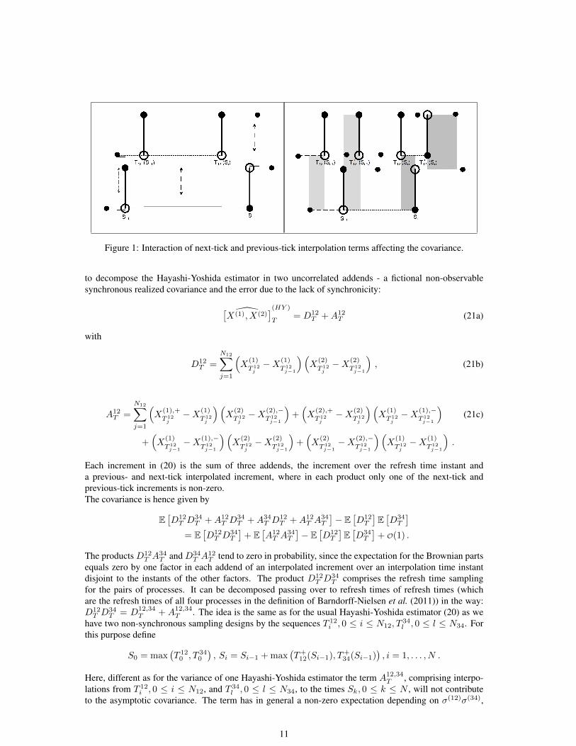
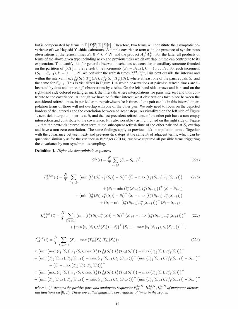
Figure 1: Interaction of next-tick and previous-tick interpolation terms affecting the covariance.
to decompose the Hayashi-Yoshida estimator in two uncorrelated addends - a fictional non-observablesynchronous realized covariance and the error due to the lack of synchronicity:
[X(1), X(2)
](HY )
T= D12
T +A12T (21a)
with
D12T =
N12∑j=1
(X
(1)
T 12j−X(1)
T 12j−1
)(X
(2)
T 12j−X(2)
T 12j−1
), (21b)
A12T =
N12∑j=1
(X
(1),+
T 12j−X(1)
T 12j
)(X
(2)
T 12j−X(2),−
T 12j−1
)+(X
(2),+
T 12j−X(2)
T 12j
)(X
(1)
T 12j−X(1),−
T 12j−1
)(21c)
+(X
(1)
T 12j−1−X(1),−
T 12j−1
)(X
(2)
T 12j−X(2)
T 12j−1
)+(X
(2)
T 12j−1−X(2),−
T 12j−1
)(X
(1)
T 12j−X(1)
T 12j−1
).
Each increment in (20) is the sum of three addends, the increment over the refresh time instant anda previous- and next-tick interpolated increment, where in each product only one of the next-tick andprevious-tick increments is non-zero.The covariance is hence given by
E[D12T D
34T +A12
T D34T +A34
T D12T +A12
T A34T
]− E
[D12T
]E[D34T
]= E
[D12T D
34T
]+ E
[A12T A
34T
]− E
[D12T
]E[D34T
]+ O(1) .
The products D12T A
34T and D34
T A12T tend to zero in probability, since the expectation for the Brownian parts
equals zero by one factor in each addend of an interpolated increment over an interpolation time instantdisjoint to the instants of the other factors. The product D12
T D34T comprises the refresh time sampling
for the pairs of processes. It can be decomposed passing over to refresh times of refresh times (whichare the refresh times of all four processes in the definition of Barndorff-Nielsen et al. (2011)) in the way:D12T D
34T = D12,34
T + A12,34T . The idea is the same as for the usual Hayashi-Yoshida estimator (20) as we
have two non-synchronous sampling designs by the sequences T 12i , 0 ≤ i ≤ N12, T
34l , 0 ≤ l ≤ N34. For
this purpose define
S0 = max(T 12
0 , T 340
), Si = Si−1 + max
(T+
12(Si−1), T+34(Si−1)
), i = 1, . . . , N .
Here, different as for the variance of one Hayashi-Yoshida estimator the term A12,34T , comprising interpo-
lations from T 12i , 0 ≤ i ≤ N12, and T 34
l , 0 ≤ l ≤ N34, to the times Sk, 0 ≤ k ≤ N , will not contributeto the asymptotic covariance. The term has in general a non-zero expectation depending on σ(12)σ(34),
11
but is compensated by terms in E[D12T
]E[D34T
]. Therefore, two terms will constitute the asymptotic co-
variance of two Hayashi-Yoshida estimators. A simple covariance term as in the presence of synchronousobservations at the refresh times Sk, 0 ≤ k ≤ N , and the product A12
T A34T . For the latter all products of
terms of the above given type including next- and previous ticks which overlap in time can contribute to itsexpectation. To quantify this for general observation schemes we consider an auxiliary structure foundedon the partition of [0, T ] in the refresh time increments (Sk − Sk−1), k = 1, . . . , N . For each increment(Sk − Sk−1), k = 1, . . . , N , we consider the refresh times T 12
i , T 34j , lain next outside the interval and
within the interval, i. e.T+12(Sk), T−12(Sk), T+
34(Sk), T−34(Sk), where at least one of the pairs equals Sk andthe same for Sk−1. This is visualized in Figure 1 in which observations at pairwise refresh times are il-lustrated by dots and “missing” observations by circles. On the left-hand side arrows and bars and on theright-hand side colored rectangles mark the intervals where interpolations for pairs intersect and thus con-tribute to the covariance. Although we have no further interest what observations take place between theconsidered refresh times, in particular more pairwise refresh times of one pair can lie in this interval, inter-polation terms of those will not overlap with one of the other pair. We only need to focus on the depictedborders of the intervals and the correlation between adjacent steps. As visualized on the left side of Figure1, next-tick interpolation terms at Si and the last precedent refresh time of the other pair have a non-emptyintersection and contribute to the covariance. It is also possible - as highlighted on the right side of Figure1 - that the next-tick interpolation term at the subsequent refresh time of the other pair and at Si overlapand have a non-zero correlation. The same findings apply to previous-tick interpolation terms. Togetherwith the covariance between next- and previous-tick steps at the same Si of adjacent terms, which can bequantified similarly as for the variance in Bibinger (2011a), we have captured all possible terms triggeringthe covariance by non-synchronous sampling.
Definition 1. Define the deterministic sequences
GN (t) =N
T
∑Si≤t
(Si − Si−1)2, (22a)
F 13,N24 (t) =
N
T
∑Si+1≤t
(min
(t+1 (Si), t
+3 (Si)
)− Si
)+ (Si −max
(t−2 (Si−1), t−4 (Si−1)
))(22b)
+(Si −min
(t−1 (Si−1), t−3 (Si−1)
))+(Si − Si−1)
+(min
(t+2 (Si), t
+4 (Si)
)− Si
)+ (Si −max
(t−1 (Si−1), t−3 (Si−1)
))+(Si −min
(t−2 (Si−1), t−4 (Si−1)
))+(Si − Si−1) ,
H13,N24 (t) =
N
T
∑Si+1≤t
(min
(t+1 (Si), t
+3 (Si)
)− Si
)+ (Si+1 −max
(t−2 (Si+1), t−4 (Si+1)
))+(22c)
+(min
(t+2 (Si), t
+4 (Si)
)− Si
)+ (Si+1 −max
(t−1 (Si+1), t−3 (Si+1)
))+,
I13,N24 (t) =
N
T
∑Si+1≤t
(Si −max
(T−12(Si), T
−34(Si)
))+(22d)
×(min
(max (t+1 (Si)), t
+3 (Si),max (t+1 (T+
12(Si)), t+3 (T34(Si)))
)−max
(T+
12(Si), T+34(Si)
))++(min
(T−12(Si−1), T−34(Si−1)
)−max
(t−1 (Si−1), t−3 (Si−1)
))+ (min
(T+
12(Si−1), T+34(Si−1)
)− Si−1
)++(Si −max
(T−12(Si), T
−34(Si)
))+×(min
(max (t+2 (Si)), t
+4 (Si),max (t+2 (T+
12(Si)), t+4 (T34(Si)))
)−max
(T+
12(Si), T+34(Si)
))++(min
(T−12(Si−1), T−34(Si−1)
)−max
(t−2 (Si−1), t−4 (Si−1)
))+ (min
(T+
12(Si−1), T+34(Si−1)
)− Si−1
)+where ( · )+ denotes the positive part, and analogous sequences F 14,N
23 , H14,N23 , I14,N
23 of monotone increas-ing functions on [0, T ]. These are called quadratic covariations of times in the sequel.
12
Assumption 3. Assume that for the sequences (22a), (22b), (22c) and (22d) from Definition 1 the followingconvergence assertions hold:
(i) GN (t) → G(t), F 13,N24 (t) → F 13
24 , F14,N23 (t) → F 14
23 , H13,N24 (t) → H13
24 (t), H14,N23 (t) → H14
23 (t),I13,N24 (t) → I13
24 (t), I14,N23 (t) → I14
23 (t) as N → ∞, where the limits are continuously differentiablefunctions on [0, T ].
(ii) For any null sequence (hN ), hN = O(N−1
)GN (t+ hN )−GN (t)
hN→ G′(t) , (23a)
F 13,N24 (t+ hN )− F 13,N
24 (t)
hN→ F 13
24′(t) , (23b)
H13,N24 (t+ hN )−H13,N
24 (t)
hN→ H13
24′(t) , (23c)
I13,N24 (t+ hN )− I13,N
24 (t)
hN→ I13
24′(t) , (23d)
uniformly on [0,T] asN →∞ and analogously forH14,N23 , F 14,N
23 , I14,N23 . The limiting functions are
called asymptotic quadratic covariations of times in the sequel.
Assumption 3, which generalizes the notion of a quadratic variation of time for the one-dimensionalcase by Zhang et al. (2005), directly postulates that sequences of time instants appearing in the sequencesof conditional covariances after applying Ito isometry and (5) converge to some limit. This is a rather weakcondition and necessary for the existence of asymptotic covariances.
Proposition 4.1. On the Assumptions 1, **2 and 3 the asymptotic covariance of two Hayashi-Yoshidaestimators is
ACOV(
[X(1), X(2)
](HY )
T, [X(3), X(4)
](HY )
T
)= T
∫ T
0
G′(s)(σ(13)s σ(24)
s + σ(14)s σ(23)
s ) ds (24)
+ T
∫ T
0
(F 13
24′+H13
24′+ I13
24′)σ(13)s σ(24)
s ds+ T
∫ T
0
(F 14
23′+H14
23′+ I14
23′)σ(23)s σ(14)
s ds .
For ‘(1) = (3)’ and ‘(2) = (4)’, we find the asymptotic variance of the Hayashi-Yoshida estimator asillustrated in Bibinger (2011a). In this case I13
24′, I14
23′ and H14
23′ are zero.
5 The general case: Asymptotic covariance matrix of the generalizedmulti-scale estimates under Asynchronicity and Microstructure
This section focuses on the general model – comprising non-synchronous sampling and noise perturbation– and an hybrid approach founded on a combination of the estimators from Sections 3 and 4.
Assumption*** 2. The process X is observed non-synchronously with additive microstructure noise:
Y(l)
t(l)j
= X(l)
t(l)j
+ ε(l)j , j = 0, . . . , nl, l ∈ 1, 2, 3, 4 .
The sequences of observation schemes are regular in the sense that n1 ∼ n2 ∼ n3 ∼ n4 and with aconstant 0 < α ≤ 1/9 it holds that
δn = sup(i,l)
((t(l)i − t
(l)i−1
), t
(l)0 , T − t(l)nl
)= O
(n−
8/9−α). (25)
The observation errors are i. i. d. sequences, independent of the efficient processes, centered and fourthmoments exist. Noise components can be mutually correlated only at synchronous observations.
13
In the following we establish the asymptotic covariance matrix for the generalized multi-scale methodfrom Bibinger (2011b) and Bibinger (2012). It arises as a convenient composition of the multi-scale real-ized (co-)variance by Zhang (2006) from Section 3 and a synchronization approach inspired by the estima-tor by Hayashi & Yoshida (2005). Virtually we can think of an idealized synchronous approximation byrefresh times, apply subsampling and the multi-scale extension to this scheme, and afterwards interpolateto the next observed values on the highest available frequency. Reviving the notation from Section 4, thegeneralized multi-scale estimator can be illustrated:
[X(1), X(2)
](multi)T
=
M(12)n∑i=1
αii
N12∑j=i
(X
(1),+
T 12j−X(1),−
T 12j−i
)(X
(2),+
T 12j−X(2),−
T 12j−i
). (26)
This estimator crucially differs from the approach by Christensen et al. (2011), which has the form of thetraditional Hayashi-Yoshida estimator, but bound to a low-frequency scheme of pre-averaged observationsover blocks of order
√n high-frequency observations. The estimator (26) relies more on the principle of
the refresh-time approximation – but contrary to Barndorff-Nielsen et al. (2011) – we use pre- and next-tickinterpolations such that the final estimator has no bias due to non-synchronicity. For this reason the articleon hand can not accomplish a unified theory that is applicable to alternative approaches by Barndorff-Nielsen et al. (2011), Aıt-Sahalia et al. (2010) and Christensen et al. (2011), since unlike their roots fromSection 3 they are not connatural any more. We consider (26) because the method attains a much smallerdiscretization variance in comparison to the one by Christensen et al. (2011), is rate-optimal and a feasiblecentral limit theorem is accessible from Bibinger (2012).
Remark 3. (Identical results for kernel estimators.) Since equations (7) and (25) are the same, it followsfrom Section 3 that our results on irregular sampling for the synchronous case, where the generalizedmulti-scale estimator (26) coincides with the original one (9), in the following apply identically to kernelestimators. Furthermore, all results for the estimator (26) apply to a generalized kernel estimator withpairwise refresh time sampling as in (26).
Definition 2. For given sampling schemes t(l)j , 0 ≤ j ≤ nl, 1 ≤ l ≤ p = 4 and r < nl, define thefunctional sequences
G(l)n,r(t) :=
nlr T
∑t(l)j ≤t
(t(l)j − t
(l)j−1)
r∧j∑q=0
(t(l)j−q − t
(l)j−q−1) , (27)
for each component and analogously for refresh times T klj , 0 ≤ j ≤ Nkl, (k, l) ∈ 1, 2, 3, 42, introducedin Section 3:
G(l,k)Nkl,r
(t) :=Nklr T
∑Tklj ≤t
(T klj − T klj−1
) r∧j∑q=0
(T klj−q − T klj−q−1
). (28)
Denote GN,r(t) as the function build in the same fashion from the refresh times of all four observed com-ponents Sj , 0 ≤ j ≤ N .
The existence of a limit G of the sequence in Definition 2 is essential to establish an asymptotic distri-bution theory, since it dominates the terms that appear in the (co-)variances of the multi-scale and relatedestimators and contribute to the asymptotic (co-)variance, namely the following existing limit:
Dα(t) := limN→∞
N
MN T
∑Sr≤t
∆Sr
MN∑i,k=1
αiαk
r∧i∧k∑q=0
(1− q
i
)(1− q
k
)∆Sr−q
. (29)
In the equidistant setupDα(t) = Dαt with the constant Dα found in Proposition 3.1. We will call the limitG in case of existence local asymptotic sampling autocorrelation (LASA). If we focus on the special case‘(1)=(2)=(3)=(4)’, convergence of (27) is assumed for the one component.
14
The preceding definition suffices to quantify the influence of non-equidistant synchronous schemes onthe asymptotic properties of the multi-scale estimator, but to give a very general asymptotic covariancestructure of the generalized multi-scale estimator in a transparent form, we can not avoid to introduce sometedious notation in the following. Readers interested mainly in the usual completely non-synchronoussetup, where the asymptotic covariances of estimates involving different components only hinge on thesignal parts, may proceed with Corollary 5.2.
Definition 3. Depending on the sequences of sampling schemes, define the following sequences of func-tions:
SN13(t) =1
N
∑t(1)j ≤t
∑t(3)k ≤t
1t(1)j =t(3)k
, (30a)
and in the same way SN14(t), SN23(t) and SN24(t). Define in the case of existence for givenM (12)N ,M
(34)N with
MN = min (M(12)N ,M
(34)N ):
S2413 = lim
N→∞N−1M−1
N
N12∑j=0
N34∑k=0
j∧M(12)N∑
r=1
k∧M(34)N∑
q=1
(1t+1 (T 12
j )=t+3 (T 34k ),t−2 (T 12
j−r)=t−4 (T 34j−q) (31a)
+1t+2 (T 12j )=t+4 (T 34
k ),t−1 (T 12j−r)=t−3 (T 34
j−q)
),
S2314 = lim
N→∞N−1M−1
N
N12∑j=0
N34∑k=0
j∧M(12)N∑
r=1
k∧M(34)N∑
q=1
(1t+1 (T 12
j )=t+4 (T 34k ),t−2 (T 12
j−r)=t−3 (T 34j−q) (31b)
+1t+2 (T 12j )=t+3 (T 34
k ),t−1 (T 12j−r)=t−4 (T 34
j−q)
),
S2413 = lim
N→∞M−1N
M(12)N −1∑j=0
M(34)N −1∑k=0
(1t+1 (T 12
j )=t+3 (T 34k ),t+2 (T 12
j )=t+4 (T 34k ) (31c)
+1t−1 (T 12N12−j)=t−3 (T 34
N34−k),t−2 (T 12N12−j)=t−4 (T 34
N34−k)
),
S2314 = lim
N→∞M−1N
M(12)N −1∑j=0
M(34)N −1∑k=0
(1t+1 (T 12
j )=t+4 (T 34k ),t+2 (T 12
j )=t+3 (T 34k ) (31d)
+1t−1 (T 12N12−j)=t−4 (T 34
N34−k),t−2 (T 12N12−j)=t−3 (T 34
N34−k)
).
Assumption* 3. Assume that for the sequences (27)/ (28) from Definition 2, and the sequences from Defi-nition 3, the following convergence assumptions hold:
(i) As N → ∞ and r → ∞ with r = O(N): GN,r(t) → G(t), for a continuous differentiable limitingfunction G on [0, T ].
(ii) For any null sequence (hN ), hN = O(N−1
):
GN,r(t+ hN )−GN,r(t)
hN→ G′(t) (32)
uniformly on [0,T] as N →∞.
(iii) SN13(t) → S13, SN14(t) → S14(t), SN23(t) → S23(t), SN24(t) → S24(t) as N → ∞, where the limits
are continuously differentiable functions on [0, T ].
15
(iv) For any null sequence (hN ), hN = O(N−1
):
SN13(t+ hN )− SN13(t)
hN→ S′13(t) ,
SN14(t+ hN )− SN14(t)
hN→ S′14(t) , (33a)
SN23(t+ hN )− SN23(t)
hN→ S′23(t) ,
SN24(t+ hN )− SN24(t)
hN→ S′24(t) , (33b)
uniformly on [0,T] as N →∞.
Proposition 5.1. On the Assumptions 1, ***2 and *3, the asymptotic covariance of generalized multi-scale estimates (26) with M (12)
n = c12
√N12 = c
√N,M
(34)n = c34
√N34 = c∗
√N , c = min (c, c∗), and
weights (10) is given by
ACOV(
[X(1), X(2)
](multi)T
, [X(3), X(4)
](multi)T
)= 2 c T
∫ T
0
(Dα)′(s)(σ(13)s σ(24)
s + σ(14)s σ(23)
s ) ds
+ c−3(S24
13C2413,αη13η24 + S23
14C2314,αη14η23
)+ c−1
(S24
13C2413,αη13η24 + S23
14C2314,αη14η23
)(34)
+ c−1Mα
∫ T
0
(η13S
′13σ
(24)s + η24S
′24σ
(13)s + η14S
′14σ
(23)s + η23S
′23σ
(14)s
)ds ,
with the existing differentiable limiting function (29) hinging on (28). All constants SC,α, SC,α depend onthe asymptotic proportion of sampling times where pairs of two components are recorded synchronouslyand the selected weights.
In a synchronous setting clearly S2413 = S23
14 = S2413 = S23
14 = 1, C2413 = C23
14 = 2Nα1 (=24 for the cubic
kernel), C2413 = C23
14 = Nα2 (=6/5 for the cubic kernel) and S′13 = S′14 = S′23 = S′24 = 1[0,T ], and (34)
coincides with (17) except the influence of irregular sampling. In particular, the asymptotic variance of themulti-scale estimator for synchronous non-equidistant sampling yields
AVAR
([
X(1), X(2)](multi)T
)= 2 c T
∫ T
0
(Dα)′(s)(σ(11)s σ(22)
s + (σ(12)s )2) ds
+ 2Nα1 c−3(η2
1η22 + η2
12
)+ c−1Mα
∫ T
0
(η2
1σ(22)s + η2
2σ(11)s + 2 η12σ
(12)s
)ds (35)
+ c−1Nα2
(η2
1η22 + η2
12
).
Interestingly, in most situations if S2413 = S23
14 = 0, the noise part will vanish. Furthermore, we obtain thefollowing important result for the completely non-synchronous case:
Corollary 5.2. In the case that no synchronous observations take place: t(l)i 6= t(k)j for all l 6= k and
(i, j) ∈ 0, . . . , nl × 0, . . . , nk, or the amount of synchronous observations tends to zero as n → ∞,using the same notation as in Proposition 5.1 and on the same (remaining) assumptions, we have:
ACOV(
[X(1), X(2)
](multi)T
, [X(3), X(4)
](multi)T
)=2 c T
∫ T
0
(Dα)′(s)(σ(13)s σ(24)
s +σ(14)s σ(23)
s ) ds , (36)
with the existing derivative of the limiting function (29).
Here, formula (36) makes sense only for different components and we may not insert ‘(1)=(3)’ orlikewise as above. However, the relation is meaningful for the asymptotic covariance between integratedvariance estimators.
Remark 4. Our major focus is not on the theoretical limits G and of other sequences, since in the generalcase they are specified only as limits. We do not need these values, however, for inference, as we shall seein the next section on feasible inference.
16
Note that convergence of (27) is the natural assumption to derive a central limit theorem for irregularlyspaced (non-equidistant) observations already in the one-dimensional framework. It emulates the asymp-totic quadratic variation of time for realized variance to an asymptotic local autocorrelation of samplingtime instants which constitutes the counterpart to the sum of squared time instants emerging in the vari-ance for subsampling and the other smoothing approaches. The only difference is that not directly the limitof (27) will appear in the asymptotic variance, but some limiting function additionally involving specificweights (the kernel). If we think of random sampling independent of Y , the structure of (27) will be partic-ularly simple for i. i. d. time instants. Virtually, only the expectation will matter and we can apply the law oflarge numbers. Assuming (32) is less restrictive than the assertion in Zhang (2006), i. e. sampling needs notto be close to an equidistant scheme in the sense that asymptotic quadratic variation of time converges to Tat T. Remarkably, for the popular model of homogenous Poisson sampling independent of X with expectedtime instants T/n, the asymptotic variance (35) is the same as for equidistant observations. This emanatesfrom the i. i. d. nature of time instants and the vanishing influence of the first addend 2T/(nr) in (27) asr →∞. The finite sample correction factor in (32) for this Poisson setup is thus (r + 1)/r.
At first glance the simple appearance of the covariance between generalized multi-scale estimates inthe typical general setup where all observations are non-synchronous and in the presence of microstruc-ture noise is intriguing. The covariance hinges only on the discretization error as if we had synchronousobservations at the refresh times Si, i = 0, . . . , N . The noise falls out of the asymptotic covariance on theassumption that observation errors at different observation times are independent.This feature constitutes another nice property of the generalized multi-scale method that not only theasymptotic variance of the estimator has a simple form, where the impact of non-synchronicity falls out inthe signal part, but the asymptotic covariances are even simpler and particularly are not influenced by thesuperposition of the four underlying different sampling schemes. Here, we benefit by the fact that for theconstruction of (26) a smoothing method to reduce noise contamination is utilized which at the same timesmoothes out interpolation effects and hence the error due to non-synchronicity.
6 A feasible multivariate stable central limit theoremIn the sequel, we conclude a feasible stable central limit theorem for linear combinations of estimatedentries of the integrated covariance matrix with estimators of the types considered above. A remainingstep towards a feasible asymptotic distribution theory allowing to draw statistical inference, is to provideconsistent estimators for the asymptotic covariances from Propositions 2.1, 3.1, 4.1 and 5.1. In the vein ofBibinger (2012), we construct consistent asymptotic covariance estimators in the general non-synchronousframework, following a histogram-type approach. For the simple case in the absence of noise and non-synchronicity, we give a simple-structured estimator resembling the prominent bipower variation.
Proposition 6.1. In the setting of Section 2, the estimator
ACOV
(n∑i=1
∆iX(1)∆iX
(2),
n∑i=1
∆iX(3)∆iX
(4)
)
=n
T
n−1∑i=1
∆iX(1)∆i+1X
(2)∆iX(3)∆i+1X
(4) + ∆i+1X(1)∆iX
(2)∆iX(3)∆i+1X
(4) , (37)
is a consistent estimator of the general asymptotic covariance according to (4).
17
On the assumptions imposed in Proposition 5.1, the estimator
ACOV(
[X(1), X(2)
](multi)T
, [X(3), X(4)
](multi)T
)
= 2 c T
KN∑j=1
∆[X(1), X(3)]n ∆[X(2), X(4)]
n
+ ∆[X(1), X(4)]n [X(2), X(3)]
n(∆DN
j
)2 DαN (T )
KN
+ c−3(S24
13C2413,αη13η24 + S23
14C2314,αη14η23
)+ c−1
(ˆS24
13ˆC24
13,αη13η24 + ˆS2314
ˆC2314,αη14η23
)(38)
+ c−1Mα
KN∑j=1
∆[X(2), X(4)]n
∆jSN13
SN13(T )
KNη13 +
KN∑j=1
∆[X(1), X(3)]n
∆jSN24
SN24(T )
KNη24
+
KN∑j=1
∆[X(1), X(4)]n
∆jSN23
SN23(T )
KNη23
KN∑j=1
∆[X(2), X(3)]n
∆jSN14
SN14(T )
KNη14
,
gives a consistent histogram-wise estimation of the general asymptotic covariance from (34). Here we use
DNj := inf t ∈ [0, T ]|Dα(t) ≥ jDα(T )/KN, 0 ≤ j ≤ KN , ∆DN
j = DNj −DN
j−1 ,
(SNlk )j := inf t ∈ [0, T ]|Slk(t) ≥ jSlk(T )/KN, 0 ≤ j ≤ KN , l = 1, 2, k = 3, 4 ,
∆jSNlk = (SNlk )j − (SNlk )j−1, 1 ≤ j ≤ KN ,
ηkl = −(N Skl(T ))−1
NSkl(T )∑i=1
∆iX(k)∆i+1X
(l), k = 1, 2, l = 3, 4 ,
and empirical realizations for all functions based on the sampling design from Definition 3. The numberof bins KN satisfies KNN
−1/3 → 0 as KN → ∞. The binwise evaluated estimators in (38) are multi-scale estimators on each bin with multi-scale frequencies MN (j), 1 ≤ j ≤ KN . One possible choice isKN = cN1/5 and MN (j) = c5/4N3/5.
Remark 5. The feasible CLT remains valid when relaxing Assumptions of Proposition 5.1 on existenceof the limit G in Assumption *3, since every subsequence of (29) has an in probability converging subse-quence, see the discussion at the end of p. 1411 in Zhang et al. (2005) for analogous reasoning and moredetails.
The estimator (38) simplifies in many cases, i. e. the completely non-synchronous setup, to the firstaddend. An estimator for the asymptotic covariance (17) of multi-scale estimators in the synchronouscase is inherent in (38) when inserting appropriate constants. One estimator for the non-noisy but non-synchronous model and the asymptotic covariance given in (24) may be constructed in a similar fashion as(38) with histogram-type estimators based on equispaced grids with respect to the quadratic covariationsof times introduced in Definition 1. Since the principle is clear from the above given estimator, we foregoto explicitly state that estimator. In the synchronous setup or for l = k, the noise (co-)variance can beestimated
√nl consistently by the realized (co-)variance or using adjacent increments as stated above.
For ‘(1) = (2) = (3) = (4)’, our estimator (37) becomes 2n∑i(∆iX)2(∆i+1X)2 and differs from
the standard estimator (2n/3)∑i(∆iX)4 proposed in Barndorff-Nielsen & Shephard (2002) which is
preferable because its variance 42 2/3n−1 is slightly smaller than 48n−1 of (37) for this case. The constantc in Proposition 6.1 is fixed from the minimum constant for the multi-scale estimates here. For an algorithmhow to select the tuning parameter adaptively involving pilot estimates to calibrate the whole estimationprocedure first, we refer to Bibinger (2012) for the generalized multi-scale and Barndorff-Nielsen et al.(2008) for the univariate kernel estimator.
18
For a quadratic symmetric (p × p) matrix A ∈ sym(p) ⊂ Rp×p, we denote the mapping to the vector ofits p(p+ 1)/2 free entries
SVEC(A) = ((Arq)1≤r≤p,1≤q≤r)>
= (A11, A12, . . . , A1p, A22, A23, . . . , A2p, . . . , Ap−1p, App)>.
Theorem 6.1. Denote [X(k), X(l)]n
, 1 ≤ k ≤ p, 1 ≤ l ≤ p, one of the integrated covariance matrix
estimators from Sections 2–5 and consider the vector SVEC
(([X(k), X(l)]
n)1≤k≤p,1≤l≤p
)of estimated
entries. The estimators fulfill a multivariate stable central limit theorem with rate rn:
rn
(SVEC
(([X(k), X(l)]
n
− [X(k), X(l)])
1≤k≤p,1≤l≤p
))stably−→ N (0,COV) , (39)
with a symmetric p(p + 1)/2 × p(p + 1)/2-dimensional asymptotic covariance matrix COV determinedby Propositions 2.1, 3.1, 4.1 and 5.1, respectively. The rate rn equals
√n, n =
∑pl=1 nl, in the non-noisy
experiment and n1/4 under microstructure noise. For linear combinations
Z :=
[∑k
ckX(k)
]n=∑k,l
ckcl[X(k), X(l)]
n
with the consistent estimators
AVAR(Z) =∑k,k,l,l
ckckclclACOV(
[X(k), X(l)]n
, [X(k), X(l)]n),
if the latter is strictly positive, a feasible central limit theorem holds:
rn
(Z/
√AVAR(Z)
)weakly−→ N (0, 1) . (40)
Note that we rescale the entries of the asymptotic covariance matrix COV from Propositions 2.1, 3.1,4.1 and 5.1, respectively, and its estimates with factors rN/rn
((N/n)(1/2) without and (N/n)(1/4) with
noise)
to obtain (39) and (40), where N denotes the number of refresh times of the involved components.The multivariate central limit theorem (39) is directly derived from the multi-dimensional version of The-orem 2–1 by Jacod (1997) which provides the basis for stable limit theorems in this research area. Byvirtue of the asymptotic covariance structure deduced in this work, it suffices to check the conditions thatcovariations of the componentwise estimation errors with the underlying reference Brownian motion Wdriving our efficient process tend to zero, as well as the covariations with all Ft-adapted bounded martin-gales orthogonal to W . The proof by establishing elementary bounds for the variances of these terms isalong the same lines as the univariate analysis, see Bibinger (2012) and Christensen et al. (2011), amongothers. Suppose without loss of generality for notational convenience that we have
(Xn, Yn)stably−→ (X,Y )
L= N
(0,
(VX CXYCXY VY
)).
By continuous mapping we conclude Xn + Yn → X + Y stably. Assume we have at hand consistentestimators V nX
p−→ VX , VnY
p−→ VY , CnXY
p−→ CXY , and set V n = V nX + V nY + 2CnXY which is assumedto be strictly positive. As V n is a bounded F-measurable random variable, stable convergence implies
(Xn + Yn, Vn)
weakly−→ (X + Y, VX + VY + 2CXY ) and hence also (Xn + Yn)/√V n
weakly−→ N (0, 1).
7 An application for conditional independence testingThis section is devoted to the design of a statistical test in order to investigate if the correlation of two assetsis only induced by a third one to which both are correlated. For multi-dimensional portfolio modeling and
19
management, information about such relations can provide valuable information and access to a new angleon the covariance structure. Conclusions in the way that a significant integrated covariance between twohigh-frequency assets might be fully explained by their dependence on a joint factor or another asset,respectively, will be of revealing impact on the used models. One interesting case we may think of is thattwo observed asset processes X1 and X2 are listed within one index recorded as high-frequency processZ. We then ask if X1 and X2 are conditionally on Z independent. To put it the other way round, pairswhich are not conditionally independent given some other asset exhibit some crucial covariance that carriesinformation about the direct mutual influence between the two assets. We understand independence herein terms of orthogonal quadratic covariation processes and will further restrict to specific hypotheses asbelow where we test for zero integrated covariances – so the term ‘independence’ is misused here for asimple illustrative phrasing. The role of Z in the model can be also some macro variable that is known orcan be estimated with faster rate. We set up a statistical experiment in which X1 and X2 are orthogonallydecomposed in the sum of Z and a process independent of Z. The constants ρX1 , ρX2 quantify the degreeof dependence on Z.
X1 = ρX1 Z + Z⊥ , X2 = ρX2 Z + Z† with [Z,Z⊥] ≡ 0 , [Z,Z†] ≡ 0 . (41)
With [X1, X2] ≡ 0 for two semimartingales X1, X2 we express that [X1, X2]s = 0 for all s ∈ [0, T ]. Forthe conditional independence hypothesis, we set
H0 : [Z⊥, Z†]T = 0 . (42)
Essentially, we do not distinguish between pairs for which the orthogonal parts are uncorrelated on thewhole line and pairs for which this correlation process integrates to zero. Our focus is on a resulting zerocovariance over [0, T ].A suitable test statistic to decide whether we rejectH0 or not is
T(X1, X2, Z) = [X1, Z]T [X2, Z]T − [X1, X2]T [Z]T , (43)
which is zero under H0. In our high-frequency framework we can estimate the single integrated covari-ances via the approaches considered in the preceding sections. The vital point is to deduce the asymptoticdistribution of the estimated version
Tn = [X1, Z]n
T[X2, Z]
n
T − [X1, X2]n
T [Z]n
T , (44)
where [ · ]n
T stands for one of the aforementioned estimators satisfying (39) whichever model fits the databest. This test statistic, though based on the simple function g(x, y, u, v) = xy − uv, is more complexto analyze than linear combinations, since we face products of our estimators. In lieu of determining thedistribution of the test statistic directly, we find help in the asymptotic covariance structure provided inthis paper and the ∆-method for stable convergence. Here, the methodology is similar to the prominentpropagation of error concept from experimental science. For each quadratic covariation, the estimationerror gets small for large n and hence we can profit when we taylor the underlying function g. Indeed, thiswill give us the leading term of the variance of Tn:
T− Tn = [X2, Z]T
([X1, Z]T − [X1, Z]
n
T
)+ [X1, Z]T
([X2, Z]T − [X2, Z]
n
T
)(45)
− [X1, X2]T
([Z]T − [Z]
n
T
)− [Z]T
([X1, X2]T − [X1, X2]
n
T
)+Op(r−4
n ) .
The asymptotic variance of the test statistic is random as we are familiar with from the usual mixed normallimits in this field. It is a linear combination of the unknown covariations we estimate and the asymptoticcovariances which are the topic of this article and can be estimated consistently as found in Proposition
20
6.1. An elementary calculation yields
AVAR(Tn) = [X2, Z]2T AVAR( [X1, Z]n
T ) + [X1, Z]2T AVAR( [X2, Z]n
T )
+ [X1, X2]2T AVAR([Z]n
T ) + [Z]2T AVAR( [X1, X2]n
T )
+ 2 [Z]T [X1, X2]TACOV( [X1, X2]n
T , [Z]n
T ) + 2 [X1, Z]T [X2, Z]TACOV( [X1, Z]n
T ,[X2, Z]
n
T )
− 2 [X1, Z]T [Z]TACOV( [X1, X2]n
T ,[X2, Z]
n
T )− 2 [X2, Z]T [Z]TACOV( [X1, X2]n
T ,[X1, Z]
n
T )
− 2 [X1, X2]T [X1, Z]TACOV( [X2, Z]n
T , [Z]n
T )− 2 [X1, X2]T [X2, Z]TACOV( [X1, Z]n
T , [Z]n
T ).
Inserting consistent estimators for the asymptotic covariances above, we finally obtain with (39) that
P0
rn TnAVAR(Tn)
weakly−→ N (0, 1) , (46)
where P0 denotes the distribution underH0 and an asymptotic distribution free test forH0.The conditional independence test also provides a tool for investigating dependencies within vast dimen-sional portfolios in order to choose small blocks, i. e. subportfolios for which covariances of the estimatesare quantified explicitly.
8 An empirical exampleWe survey our methods in an application study on NASDAQ intra-day trading data, reconstructed fromfirst-level order book data, from August 2010. We consider a sample portfolio with 5 assets, namely Apple(AAPL), Microsoft (MSFT), Oracle (ORCL), Exxon Mobil Corporation (XOM) and Pfizer (PFE). Wequantify the complete asymptotic covariance matrix of generalized multi-scale estimates with weights (16)for the integrated covariance matrix over the whole month (where we discard over-night returns) and forthe first trading day, 2010/08/02. The data provides a good training data set to analyze estimation and testprocedures.For a p-dimensional portfolio, the number of free entries of the symmetric covariance matrix is given by
1
2
p(p+ 1)
2
(p(p+ 1)
2+ 1
)= p+ 3
(p
4
)+ 3 · 2
(p
3
)+ 4
(p
2
). (47)
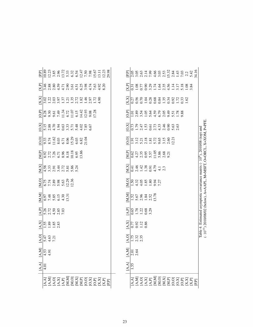
The left-hand illustration is derived by the reasoning that we estimate p(p + 1)/2 different entries of thesymmetric integrated covariance matrix which leads to a (p(p + 1)/2)2-dimensional covariance matrixwhich is symmetric again. Since the dimension of the asymptotic covariance matrix increases proportionalto p4, an evaluation of all covariances is tractable only for small values of p (our estimates of risk in ap-dimensional portfolio have dimension proportional to p2 and the risk of the estimates proportional to p4).In Table 3, we list the estimates for integrated covariances ± estimated standard deviation. With the esti-mators (38) and the numbers of refresh times of incorporated components, we quantify covariances of thegeneralized multi-scale estimates which are listed in Table 4. The bottom line is that involving asymptoticcovariances is indispensable when facing questions for multivariate portfolio management. The estimatedquadratic variation of a sum of all five assets is (41.57±0.26) ·10−3 for 2010/08 and (129.22±6.88) ·10−5
for 2010/08/02. The estimated asymptotic variances, 6.93 · 10−8 and 47.42 · 10−10, are mainly inducedby estimated covariance terms (6.34/42.91), whereas the trace of the matrix, i. e. the sum of estimates forasymptotic variances, is smaller. If one would mistakenly act as if the estimators were uncorrelated, thisleads to a tremendous underestimate of the estimation risk. Note that in principle, e. g. for negativelycorrelated assets, the risk could sometimes also decrease by adding covariances. For [MSFT+ORCL],which have the highest correlation in our portfolio, the ratios of the estimated sum of variances to the es-timated sum of all covariances are 0.14/0.45 and 0.85/3.30, respectively, and for the least correlated pairs,[AAPL+XOM] and [PFE+XOM], respectively, we have 0.09/0.20 and 0.84/1.59.We perform the test from Section 7, to investigate three hypotheses: if MSFT and ORCL have a zero co-variation conditional on PFE; ORCL and PFE conditional on MSFT and MSFT and PFE conditional on
21
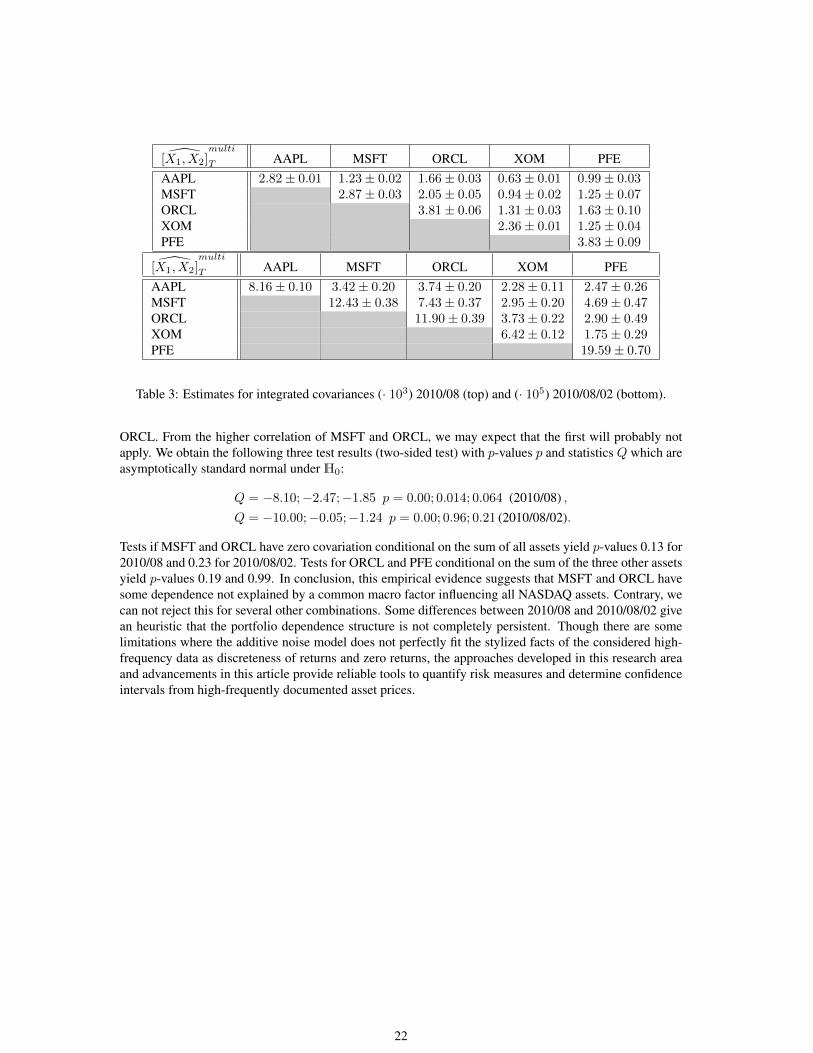
[X1, X2]multi
T AAPL MSFT ORCL XOM PFEAAPL 2.82± 0.01 1.23± 0.02 1.66± 0.03 0.63± 0.01 0.99± 0.03MSFT 2.87± 0.03 2.05± 0.05 0.94± 0.02 1.25± 0.07ORCL 3.81± 0.06 1.31± 0.03 1.63± 0.10XOM 2.36± 0.01 1.25± 0.04PFE 3.83± 0.09
[X1, X2]multi
T AAPL MSFT ORCL XOM PFEAAPL 8.16± 0.10 3.42± 0.20 3.74± 0.20 2.28± 0.11 2.47± 0.26MSFT 12.43± 0.38 7.43± 0.37 2.95± 0.20 4.69± 0.47ORCL 11.90± 0.39 3.73± 0.22 2.90± 0.49XOM 6.42± 0.12 1.75± 0.29PFE 19.59± 0.70
Table 3: Estimates for integrated covariances (· 103) 2010/08 (top) and (· 105) 2010/08/02 (bottom).
ORCL. From the higher correlation of MSFT and ORCL, we may expect that the first will probably notapply. We obtain the following three test results (two-sided test) with p-values p and statistics Q which areasymptotically standard normal underH0:
Q = −8.10;−2.47;−1.85 p = 0.00; 0.014; 0.064 (2010/08) ,Q = −10.00;−0.05;−1.24 p = 0.00; 0.96; 0.21 (2010/08/02).
Tests if MSFT and ORCL have zero covariation conditional on the sum of all assets yield p-values 0.13 for2010/08 and 0.23 for 2010/08/02. Tests for ORCL and PFE conditional on the sum of the three other assetsyield p-values 0.19 and 0.99. In conclusion, this empirical evidence suggests that MSFT and ORCL havesome dependence not explained by a common macro factor influencing all NASDAQ assets. Contrary, wecan not reject this for several other combinations. Some differences between 2010/08 and 2010/08/02 givean heuristic that the portfolio dependence structure is not completely persistent. Though there are somelimitations where the additive noise model does not perfectly fit the stylized facts of the considered high-frequency data as discreteness of returns and zero returns, the approaches developed in this research areaand advancements in this article provide reliable tools to quantify risk measures and determine confidenceintervals from high-frequently documented asset prices.
22
[A,A
][A
,M]
[A,O
][A
,X]
[A,P
][M
,M]
[M,O
][M
,X]
[M,P
][O
,O]
[O,X
][O
,P]
[X,X
][X
,P]
[P,P
][A
,A]
4.01
4.53
5.47
1.55
5.26
6.97
6.75
4.58
6.92
9.33
5.15
8.28
3.02
3.46
10.8
9[A
,M]
4.91
4.63
1.89
2.72
7.48
7.74
3.33
2.72
8.74
2.88
9.30
1.22
2.88
12.2
3[A
,O]
7.21
1.85
4.50
5.85
2.89
2.91
7.26
11.6
24.
709.
612.
032.
803.
85[A
,X]
2.83
2.85
6.15
5.98
3.44
6.71
8.03
1.94
7.49
3.97
4.59
2.96
[A,P
]7.
034.
305.
632.
728.
966.
710.
6311
.34
1.37
4.71
13.7
2[M
,M]
13.3
112
.29
5.81
8.18
8.06
3.33
6.72
1.21
2.90
5.33
[M,O
]12
.36
5.86
10.1
815
.29
5.71
11.0
71.
353.
616.
32[M
,X]
5.24
6.95
6.03
5.48
6.15
2.72
4.51
6.54
[M,P
]13
.86
6.82
4.02
14.4
21.
826.
2512
.47
[O,O
]21
.04
7.85
12.9
31.
463.
987.
50[O
,X]
6.67
9.08
2.97
4.74
7.98
[O,P
]17
.28
1.72
7.63
15.6
7[X
,X]
4.90
4.92
13.1
1[X
,P]
8.20
12.2
3[P
,P]
29.9
8
[A,A
][A
,M]
[A,O
][A
,X]
[A,P
][M
,M]
[M,O
][M
,X]
[M,P
][O
,O]
[O,X
][O
,P]
[X,X
][X
,P]
[P,P
][A
,A]
1.55
2.01
1.75
0.77
0.65
1.52
1.50
0.41
0.62
1.91
0.73
1.01
0.27
0.31
2.05
[A,M
]2.
642.
320.
921.
785.
674.
322.
464.
273.
121.
792.
890.
561.
083.
05[A
,O]
2.35
1.12
1.22
2.96
4.05
1.42
2.35
5.21
2.47
3.54
0.70
0.77
2.63
[A,X
]0.
860.
681.
841.
851.
380.
952.
181.
531.
051.
040.
902.
14[A
,P]
3.29
2.52
1.80
0.91
5.57
1.81
0.61
5.64
0.28
3.29
7.99
[M,M
]13
.78
9.94
4.79
11.0
55.
722.
734.
590.
681.
744.
66[M
,O]
7.27
4.1
5.86
9.65
4.33
6.79
0.84
1.64
3.03
[M,X
]2.
32.
683.
152.
462.
051.
352.
352.
53[M
,P]
9.21
2.60
0.90
9.49
0.34
4.56
15.3
2[O
,O]
12.2
15.
635.
510.
921.
142.
84[O
,X]
2.63
1.78
1.72
3.17
1.43
[O,P
]9.
880.
335.
187.
03[X
,X]
1.62
1.08
2.2
[X,P
]3.
845.
42[P
,P]
34.1
6Ta
ble
4:E
stim
ated
asym
ptot
icco
vari
ance
mat
rix
(·108),
2010
/08
(top
)and
(·1010)2
010/
08/0
2(b
elow
),A
=AA
PL,M
=MSF
T,O
=OR
CL
,X=X
OM
,P=P
FE.
23
AcknowledgementsThe authors would like to thank Dacheng Xiu, Ruey Tsay and Dan Christina Wang for inspiring discus-sions. We also thank Johannes Schmidt-Hieber and Till Sabel for a discussion on the relation of estimatorsvia quadratic forms for noise smoothing who have worked on the transformations between several of theseestimators.Markus Bibinger was supported by a fellowship within the Postdoc-Programme of the German AcademicExchange Service (DAAD) and the CRC 649 ‘Economic Risk’ at Berlin, supported by the DeutscheForschungsgemeinschaft (DFG), and also from the Stevanovich Center for Financial Mathematics at theUniversity of Chicago. Per Mykland was supported under National Science Foundation grant SES 11-24526. We gratefully acknowledge this financial support.The NASDAQ trading data used in Section 8 has been reconstructed from the order book with LOBSTERprovided by the high-frequency econometrics team at the Chair of Econometrics, School of Business andEconomics, Humboldt-Universitat zu Berlin, Germany.
ReferencesAıt-Sahalia, Y., J. Fan, & D. Xiu (2010). High-frequency estimates with noisy and asynchronous financial
data. Journal of the American Statistical Association 105(492), 1504–1516.
Aıt-Sahalia, Y., L. Zhang, & P. A. Mykland (2011). Ultra high frequency volatility estimation with depen-dent microstructure noise. Journal of Econometrics, 160, 160–165.
Andersen, T. G. & T. Bollerslev (1998). Answering the skeptics: Yes, standard volatility models do provideaccurate forecasts. International Economic Review 39, 885–905.
Andersen, T. G., T. Bollerslev, F. X. Diebold, & P. Labys (2000). Great realizations. Risk 13, 105–108.
Andersen, T. G., T. Bollerslev, F. X. Diebold, & P. Labys (2001). The distribution of realized exchange ratevolatility. Journal of the American Statistical Association 96, 42–55.
Andersen, T. G., T. Bollerslev, F. X. Diebold, & P. Labys (2003). Modeling and forecasting realizedvolatility. Econometrica 71, 579–625.
Barndorff-Nielsen, O. E., P. R. Hansen, A. Lunde, & N. Shephard (2008). Designing realised kernels tomeasure the ex-post variation of equity prices in the presence of noise. Econometrica 76(6), 1481–1536.
Barndorff-Nielsen, O. E., P. R. Hansen, A. Lunde, & N. Shephard (2011). Multivariate realised ker-nels: consistent positive semi-definite estimators of the covariation of equity prices with noise and non-synchronous trading. Journal of Econometrics 162(2), 149–169.
Barndorff-Nielsen, O. E. & N. Shephard (2001). Non-Gaussian Ornstein-Uhlenbeck-based models andsome of their uses in financial economics. Journal of the Royal Statistical Society, B 63, 167–241.
Barndorff-Nielsen, O. E. & N. Shephard (2002). Econometric analysis of realized volatility and its use inestimating stochastic volatility models. Journal of the Royal Statistical Society 64(2), 253–280.
Bibinger, M. (2011a). Asymptotics of asynchronicity. Technical Report, Humboldt-Universitat zu Berlin,URL=http://sfb649.wiwi.hu--berlin.de/papers/pdf/SFB649DP2011--033.pdf.
Bibinger, M. (2011b). Efficient covariance estimation for asynchronous noisy high-frequency data. Scan-dinavian Journal of Statistics 38, 23–45.
Bibinger, M. (2012). An estimator for the quadratic covariation of asynchronously observed ito processeswith noise: Asymptotic distribution theory. Stochastic Processes and their Applications 122, 2411–2453.
24
Bibinger, M., M. Reiß, N. Hautsch, & P. Malec (2012). Asymptotically efficient covolatility matrix esti-mation via local likelihoods. preprint, HU Berlin.
Black, F. S. & M. S. Scholes (1973). The pricing of options and corporate liabilities. Journal of PoliticalEconomy 81, 637–654.
Christensen, K., S. Kinnebrock, & M. Podolskij (2010). Pre-averaging estimators of the ex-post covariancematrix in noisy diffusion models with non-synchronous data. Journal of Econometrics, 159(1), 116–133.
Christensen, K., M. Podolskij, & M. Vetter (2011). On covariation estimation for multivariate continuousito semimartingales with noise in non-synchronous observation schemes. CREATES research paper2011-53.
Eberlein, E., R. Frey, & E. A. von Hammerstein (2008). Advanced credit portfolio modeling and cdopricing. In Mathematics – Key Technology for the Future, edited by W. Jager and H.-J. Krebs, Springer,253–280.
Epps, T. W. (1979). Comovements in stock prices in the very short run. Journal of the American StatisticalAssociation 74, 291–298.
Gloter, A. & J. Jacod (2001). Diffusions with measurement errors 1 and 2. ESAIM Probability andStatistics 5, 225–242.
Harrison, M. & D. Kreps (1979). Martingales and arbitrage in multiperiod securities markets. Journal ofEconomic Theory 20, 381–408.
Harrison, M. & S. Pliska (1981). Martingales and stochastic integrals in the theory of continuous trading.Stochastic Processes and Their Applications 11, 215–260.
Hayashi, T. & N. Yoshida (2005). On covariance estimation of non-synchronously observed diffusionprocesses. Bernoulli 11(2), 359–379.
Hayashi, T. & N. Yoshida (2011). Nonsynchronous covariation process and limit theorems. StochasticProcesses and their Applications 121, 2416–2454.
Heston, S. L. (1993). A closed-form solution for options with stochastic volatility with applications tobond and currency options. Review of Financial Studies 6, 327–343.
Isserlis, L. (1918). On a formula for the product-moment coefficient of any order of a normal frequencydistribution in any number of variables. Biometrika 12, 134–139.
Jacod, J. (1997). On continuous conditional gaussian martingales and stable convergence in law. Seminairede Probabilities, Strasbourg, tome 31, 232–246.
Jacod, J. (2012). Statistics and high frequency data. Proceedings of the 7th Seminaire Europeen de Statis-tique, La Manga, 2007: Statistical methods for stochastic differential equations, edited by M. Kessler, A.Lindner and M. Sørensen.
Jacod, J., Y. Li, P. A. Mykland, M. Podolskij, & M. Vetter (2009). Microstructure noise in the continouscase: the pre-averaging approach. Stochastic Processes and their Applications 119, 2803–2831.
Jacod, J. & P. Protter (1998). Asymptotic error distributions for the euler method for stochastic differentialequations. The Annals of Probability 26, 267–307.
Mykland, P. & L. Zhang (2012). The econometrics of high frequency data. Proceedings of the 7th SeminaireEuropeen de Statistique, La Manga, 2007: Statistical methods for stochastic differential equations,edited by M. Kessler, A. Lindner and M. Sørensen.
Mykland, P. A. (2012). A gaussian calculus for inference from high frequency data. Annals of Finance 8,235–258.
25
Mykland, P. A., N. Shephard, & K. Sheppard (2012). Efficient and feasible inference for the componentsof financial variation using blocked multipower variation. Technical Report, University of Oxford.
Mykland, P. A. & L. Zhang (2009). Inference for continuous semimartingales observed at high frequency.Econometrica 77, 1403–1455.
Park, S. & O. Linton (2012). Estimating the quadratic covariation matrix for an asynchronously observedcontinuous time signal masked by additive noise. FMG Discussion Papers 703.
Renyi, A. (1963). On stable sequences of events. Sankhya: The Indian Journal of Statistics, Series A 25(3),293–302.
Rootzen, H. (1980). Limit distributions for the error in approximations of stochastic integrals. Annals ofProbability 8, 241–251.
Ross, S. M. (1976). The arbitrage theory of capital asset pricing. Journal of Economic Theory 13, 341–360.
Xiu, D. (2010). Quasi-maximum likelihood estimation of volatility with high frequency data. Journal ofEconometrics 159, 235–250.
Zhang, L. (2001). From Martingales to ANOVA: Implied and Realized Volatility. Ph. D. thesis, TheUniversity of Chicago, Department of Statistics.
Zhang, L. (2006). Efficient estimation of stochastic volatility using noisy observations: A multi-scaleapproach. Bernoulli 12(6), 1019–1043.
Zhang, L. (2011). Estimating covariation: Epps effect and microstructure noise. Journal of Economet-rics 160, 33–47.
Zhang, L., P. A. Mykland, & Y. Aıt-Sahalia (2005). A tale of two time scales: Determining integratedvolatility with noisy high-frequency data. Journal of the American Statistical Association 100(472),1394–1411.
26
APPENDIX: PROOFS
A Proofs
A.1 PreliminariesThe local boundedness condition in Assumption 1 can be strengthened to uniform boundedness on [0, T ]by a localization procedure carried out in Jacod (2012), Lemma 6. 6 of Section 6 .3. Let C be a genericconstant and denote ∆iW = WiT/n −W(i−1)T/n, i = 1, . . . , n, for the Brownian motion W driving theSDE with solution X in (1) and ∆iσ = σiT/n − σ(i−1)T/n. Consider some norm ‖ · ‖, e. g. the euclideannorm, on Rp. Suppose Assumption 1 holds. By several applications of the Burkholder-Davis-Gundy andHolder inequality one can obtain the following estimates:
E[‖∆iX‖2 + ‖∆iW‖2
∣∣F(i−1)/n
]≤ Cn−1, E
[‖∆iσ‖2
∣∣F(i−1)/n
]≤ Cn−1 , (A.1a)
E[‖∆iX −∆iW‖2
∣∣F(i−1)/n
]≤ Cn−2 , (A.1b)
for equidistant observation schemes. For general synchronous sampling (A.1a) and (A.1b) remain validwhen replacing n by δ−1
n with δn = supi (ti − ti−1). The estimates (A.1a) and (A.1b) are proven in Jacod(2012), among others. They are used repeatedly in the analysis below. We will as well make use of thedirect extensions for increments with respect to subsampled time lags and the componentwise versions of(A.1a) and (A.1b).Recall (6), which is a special case of the result by Isserlis (1918) and used implicitly throughout the proofsbelow. For notational convenience we write again an ∼p bn if an = Op(bn) and bn = Op(an).
A.2 Proof of Proposition 2.1Applying (6) and (A.1b), by the Ito isometry we deduce for the random conditional covariance
CovΣ
(n∑i=1
∆iX(1)∆iX
(2),
n∑i=1
∆iX(3)∆iX
(4)
)∼p
n∑i=1
Covi−1
(∆iX
(1)∆iX(2),∆iX
(3)∆iX(4))
∼pn∑i=1
(σ
(13)(i−1)T
n
σ(24)(i−1)T
n
+ σ(14)(i−1)T
n
σ(23)(i−1)T
n
)T 2
n2,
where we write Covi−1( · ) for Cov( · |F(i−1)T/n) and CovΣ( · ) for the random covariance dependent onΣ. By convergence of the Riemann sum to the integral, this yields
nCovΣ
(n∑i=1
∆iX(1)∆iX
(2),
n∑i=1
∆iX(3)∆iX
(4)
)p−→ T
∫ T
0
(σ(13)s σ(24)
s + σ(14)s σ(23)
s
)ds .
A.3 Proof of Theorem 3.1For the proof that(
[X(1), X(2)
](multi)T
− [X(1), X(2)
](kernel)T
)= −4η12 + Op
(n−
1/4)
27
if K′′ = h in (10), it suffices to focus on the first-order term of the weights. Transforming (9) yields
Mn∑i=1
αii
n∑j=i
∆ijY
(1)∆ijY
(2) =
Mn∑i=1
αi
n∑j=2
i∧(j−1)∑l=1
(1− l
i
)(∆jY
(1)∆j−lY(2) + ∆jY
(2)∆j−lY(1))
+
n∑j=1
∆jY(1)∆jY
(2) −Rn
=
Mn∑l=1
n∑j=l+1
Mn∑i=l
αi
(1− l
i
)(∆jY
(1)∆j−lY(2) + ∆jY
(2)∆j−lY(1))
+
n∑j=1
∆jY(1)∆jY
(2) −Rn
where we suppress additional component superscripts on Mn. The term Rn induced by end-effects
Mn∑i=1
αi
i−1∑j=1
i− ji
∆jY(1)∆jY
(2) +
(j−1)∧1∑l=1
i− ji
(∆jY(1)∆j−lY
(2) + ∆jY(2)∆j−lY
(1))
+
n∑j=n−i+2
i− n+ j − 1
i
∆jY(1)∆jY
(2)+
i∧(n−j)∑l=1
(∆jY(1)∆j−lY
(2) + ∆jY(2)∆j−lY
(1))
has an expectation by noise:
η12
Mn∑i=1
αi
i−1∑j=1
i− ji−
i−1∑j=2
i− ji
+
n−1∑j=n−i+1
i− n+ j
i−
n−2∑j=n−i+1
i− n+ j
i
= 4η12 .
The variance of this term is negligible which can be shown with standard bounds. For the main term above,we can detach the inner sum and find that
Mn∑i=l
αi
(1− l
i
)=
Mn∑i=l
i
M2n
(i− l)i
K′′(
i
Mn
)+ O
(n−
1/4)
=
∫ 1
l/Mn
K′′(x)
(x− l
Mn
)dx+ O
(n−
1/4)
= K
(l
Mn
)+ O
(n−
1/4),
by partial integration under the restrictions made on K. This yields the form (11) of the transformed kernelestimator and our claim. That the integral approximation does not harm the above equality up to theO(n−1/4
)-term, can be seen by the estimate∫ (i+1)/Mn
i/Mn
∣∣∣∣f(x)− f(
i
Mn
)∣∣∣∣ dx ≤ ∫ (i+1)/Mn
i/Mn
C
∣∣∣∣x− i
Mn
∣∣∣∣ dx ≤ CM−2n
with generic constant C, i ≥ l, for the Lipschitz function
f(x) = K′′(x)
(x− l
Mn
)on the compact support [0, 1], where Lipschitz continuity is ensured by the preconditioned continuousdifferentiability.
28
A.4 Proof of Proposition 3.1Decompose the multi-scale estimator (9) for [X(k), X(l)]T , (k, l) ∈ 1, 2, 3, 42
M(kl)n∑i=1
αii
n∑j=i
∆ijY
(l)∆ijY
(k) =
M(kl)n∑i=1
αii
n∑j=i
∆ijX
(l)∆ijX
(k) +
M(kl)n∑i=1
αii
n∑j=i
∆ijε
(l)∆ijε
(k)
+
M(kl)n∑i=1
αii
n∑j=i
∆ijX
(l)∆ijε
(k) +
M(kl)n∑i=1
αii
n∑j=i
∆ijε
(l)∆ijX
(k) ,
with ∆ji ε
(l) analogously defined as for X(l), in a signal part, a noise part and cross terms which are uncor-related for each component. We analyze the covariances which stem from covariances of the signal, noiseparts and cross terms consecutively. The elements of the proof of a stable central limit theorem is similaras in Zhang (2006) and Bibinger (2012), respectively, and hence we restrict ourselves to the evaluation ofthe general covariance including possibly different frequencies and weights for equidistant sampling.We can write the signal part of the addends of [X(1), X(2)]T in the way
1
i12
n∑j=i12
∆i12j X(1)∆i12
j X(2) =
n∑j=1
∆jX(1)∆jX
(2) +
n∑l=1
∆lX(1)
i12∧l∑j=1
(1− j
i12
)∆l−jX
(2)
+
n∑l=1
∆lX(2)
i12∧l∑j=1
(1− j
i12
)∆l−jX
(1) .
The first addend is the usual realized covariance and will contribute only asymptotically negligible covari-ance terms in the noisy setting with slower convergence rate. We derive that
CovΣ
1
i12
n∑j=i12
∆i12j X(1)∆i12
j X(2),1
i34
n∑j=i34
∆i34j X(3)∆i34
j X(4)
∼p Γn13 + Γn14 + Γn23 + Γn24 ,
with conditional covariance terms
Γn13 =
n∑l=1
E[∆lX
(1)∆lX(3)]min (i12,i34,l)∑
j=1
(1− j
i12
)(1− j
i34
)∆l−jX
(2)∆l−jX(4)
∼pn∑l=1
σ(13)(l−1)T
n
1
n
min (i12,i34,l)∑j=1
(1− j
i12
)(1− j
i34
)σ
(24)(l−1)T
n
1
n, (A.2)
and analogously for the other addends. The smoothness of Σ ensured by Assumption 1 giving the boundin (A.1a) suffices that we can approximately take σ(24)
(l−1)T/n in all addends of the second sum. Hence, forthe equidistant case the analysis boils down to simply evaluating the deterministic inner sum:
m∑j=1
(1− j
i12
)(1− j
i34
)=m
2− m2
6M− 1
8+
1
12M∼ m
6
(3− m
M
),
where m = min (i12, i34) and M = max (i12, i34). For Mn = min(M
(12)n ,M
(34)n
)denote the limit of
the following series including weights according to (10)
Dα = limn→∞
M−1n
Mn∑k=1
k∑l=1
l
6Mn
(3− l
k
)αkαl .
This leads to the result
n
Mn
Mn∑i12,i34=1
αi12αi34Γn13p−→ Dα T
∫ T
0
σ(13)s σ(24)
s ds .
29
Similar results hold for Γn14,Γn23,Γ
n24. Thereby we conclude the signal term of (17). Dα is a constant
showing up in the asymptotic discretization variance depending on the weights, where for the standardweights (16) or cubic kernel Dα = 13/70. Eventually, we also obtain the general form of the asymptoticdiscretization variance of the one-dimensional estimator.The addend induced by market microstructure noise in the multi-scale estimator (9) is
M(12)n∑i=1
αii
n∑j=i
(ε(1)j − ε
(1)j−i
)(ε(2)j − ε
(2)j−i
)=
M(12)n∑i=1
αii
2
n∑j=1
ε(1)j ε
(2)j
−n∑j=i
(ε(1)j ε
(2)j−i + ε
(2)j ε
(1)j−i
)−
n∑j=n−i+1
ε(1)j ε
(2)j −
i−1∑j=0
ε(1)j ε
(2)j
.
The last two sums lead for the non-adjusted multi-scale estimator (9) to the negative bias by noise and end-effects. We have focused on the bias and an adjusted corrected estimator in Section 3 and will concentrateon the adjusted non-biased version in the sequel. The first inner sum on the right-hand side does not
depend on i and vanishes since∑M(12)
ni=1 αi/i = 0. The covariances of the remaining uncorrelated addends
contribute to the total covariance due to noise perturbation. Denote the constant limits
Nα2 = lim
n→∞Mn
Mn−1∑j=1
Mn∑i=j+1
αii
2
and Nα1 = lim
n→∞M3n
Mn∑i=1
α2i
i2
and rewriting
M(12)n∑i=1
αii
n∑j=i
ε(1)j ε
(2)j−i =
n∑j=i
M(12)n ∧j∑i=1
αiiε(1)j ε
(2)j−i
and also
M(12)n∑i=1
αii
i−1∑j=0
ε(1)j ε
(2)j +
n∑j=n−i+1
ε(1)j ε
(2)j
=
M(12)n −1∑j=0
(ε(1)j ε
(2)j + ε
(1)n−jε
(2)n−j
) M(12)n∑
i=j+1
αii,
we obtain with Mn = min(M
(12)n ,M
(34)n
)that
√M3n
nCov
M(12)n∑i=1
αii
n∑j=i
ε(1)j ε
(2)j−i,
M(34)n∑i=1
αii
n∑j=i
ε(3)j ε
(4)j−i
−→ Nα1 η13η24 , (A.3)
and that
√MnCov
M(12)n∑i=1
αii
n∑j=n−i+1
ε(1)j ε
(2)j +
i−1∑j=0
ε(1)j ε
(2)j ,
M(34)n∑i=1
αii
n∑j=n−i+1
ε(3)j ε
(4)j +
i−1∑j=0
ε(3)j ε
(4)j
−→ Nα
2 (η13η24 + η14η23) . (A.4)
The analogous implications for all addends contributing to the total covariance by noise lead to the noiseparts in (17). For (16), we have Nα
2 = 6/5 and Nα1 = 12, which gives the minimum of the variance due to
noise (see Zhang (2006)). Note that for the weights from (10), the respective frequencies M (kl)n , 1 ≤ k ≤
4, 1 ≤ l ≤ 4, are inserted, but we leave out further indices for a better readability.Finally, consider the cross terms of (9). They can be decomposed in addends of the form
M(kl)n∑i=1
αii
n∑j=0
ζ(k)i,j ε
(l)j (A.5)
30
for components (k, l), where
ζ(k)i,j =
−∆i
i−jX(k) , 0 ≤ j ≤ (i− 1)
∆ijX
(k) −∆ij+iX
(k) , i ≤ j ≤ (n− i)∆ijX
(k) , n− i+ 1 ≤ j ≤ n.
The asymptotic covariance coming from cross terms, by the martingale structure of the above term can bededuced by the limit of the sum over j covariances conditionally on FT
∨σ (εl, l ≤ j − 1). We thus have
CovΣ
M(12)n∑i=1
αii
n∑j=0
ζ(1)i,j ε
(2)j ,
M(34)n∑i=1
αii
n∑j=0
ζ(3)i,j ε
(4)j
=
n∑j=0
E[ε(1)j ε
(3)j
]M(12)n∑i=1
αiiζ
(2)i,j
M(34)n∑i=1
αiiζ
(4)i,j .
Now, similarly as in Zhang (2006) and Bibinger (2012), if we assume without loss of generality 1 ≤ i12 ≤i34 ≤Mn = min
(M
(12)n ,M
(34)n
), it holds that
ζ(k)i12,j
ζ(l)i34,j
=
j−1∑r=j−i12
∆rX(k) −
i12+j−1∑r=j
∆rX(k)
j−1∑r=j−i34
∆rX(l) −
i34+j−1∑r=j
∆rX(l)
= ζ
(k)i12ζ
(l)i12
+ ζ(k)i34
j−i12−1∑r=j−i34
∆rX(l) −
i34+j−1∑r=j+i12
∆rX(l)
k = 1, 2; l = 3, 4.
The conditional covariances from these addends yield for u, k, l, v ∈ 1, 2, 3, 4
MnCovΣ
M(12)n∑i=1
αii
n∑j=0
ζ(k)i,j ε
(u)j ,
M(34)n∑i=1
αii
n∑j=0
ζ(l)i,j ε
(v)j
∼p 2Mnηuv
Mn∑i=1
Mn∑r=1
αiαrir
(i ∧ r)
1
(i ∧ r)
n∑j=(i∧r)
∆(i∧r)j X(k)∆
(i∧r)j X(l)
p−→Mαηuv
[X(k), X(l)
]T.
For the specific weights (16), the constant takes the value Mα = 6/5. This leads to the total covariance bycross terms completing the proof and we conclude Proposition 3.1.
A.5 Proof of Proposition 4.1Recall the illustration (20) of the Hayashi-Yoshida estimator with refresh times and interpolations. We firstconsider the term D12
T D34T from the product of the two synchronous-type approximations. Only overlap-
ping increments contribute to the asymptotic covariance:
E[D12T D
34T
]=∑i,j
1max (T 12i−1,T
34j−1)<min (T 12
i ,T 34j )
× E[(X
(1)
T 12i−X(1)
T 12i−1
)(X
(2)
T 12i−X(2)
T 12i−1
)(X
(3)
T 34j−X(3)
T 34j−1
)(X
(4)
T 34j−X(4)
T 34j−1
)]and thus
Cov(D12T , D
34T ) =
N∑i=1
Cov((X
(1)Si−X(1)
Si−1
)(X
(2)Si−X(2)
Si−1
),(X
(3)Si−X(3)
Si−1
)(X
(4)Si−X(4)
Si−1
)).
Only on intervals where increments of all four processes coincide, the expectation of the product with fourfactors does not equal the product of expectations. For that reason the refresh times Si, i = 0, . . . , N , of all
31
processes give the crucial synchronous approximation here. The other remaining addend is the covarianceof the terms due to non-synchronicity for each pair A12
T A34T . We have that
E[A12T A
34T
]=∑i,j
1max (t−1 (T 12i−1),t−2 (T 12
i−1),t−3 (T 34j−1),t−4 (T 34
j−1))<min (t+1 (T 12i ),t+2 (T 12
i ),t+3 (T 34j ),t+4 (T 34
j ))
× Cov((X
(1),+
T 12i−X(1)
T 12i
+X(1)
T 12i−1−X(1),−
T 12i−1
)(X
(2),+
T 12i−X(2)
T 12i
+X(2)
T 12i−1−X(2),−
T 12i−1
),(
X(3),+
T 34j−X(3)
T 34j
+X(3)
T 34j−1−X(3),−
T 34j−1
)(X
(4),+
T 34j−X(4)
T 34j
+X(4)
T 34j−1−X(4),−
T 34j−1
))As explained in Section 3, we can arrange the coinciding interpolation terms using the structuring generatedby the Sis. Consider now the sequence of covariances conditionally on FSi−1
, i = 1, . . . , N , and its sum.For the first term with the synchronous approximation this is
N∑i=1
Cov((X
(1)Si−X(1)
Si−1
)(X
(2)Si−X(2)
Si−1
),(X
(3)Si−X(3)
Si−1
)(X
(4)Si−X(4)
Si−1
) ∣∣FSi−1
)∼p
N∑i=1
(σ
(13)Si−1
σ(24)Si−1
+ σ(14)Si−1
σ(23)Si−1
)(Si − Si−1)2
=
N∑i=1
(σ
(13)Si−1
σ(24)Si−1
+ σ(14)Si−1
σ(23)Si−1
) (G(Si)−G(Si−1))
Si − Si−1(Si − Si−1)
and analogously for Cov(A12T , A
34T ) with all interpolations. The difference quotients will converge on
Assumption 3 and the Riemann sums to the corresponding integrals. With all functions from Definition 1and Assumption 3, we obtain
ACOV = p− limN→∞
(N∑i=1
(σ
(13)Si−1
σ(24)Si−1
+ σ(14)Si−1
σ(23)Si−1
) (G(Si)−G(Si−1))
Si − Si−1(Si − Si−1)
+
N∑i=1
σ(13)Si−1
σ(24)Si−1
(F 1324 (Si)−F 13
24 (Si−1))+(H1324 (Si)−H13
24 (Si−1))+(I1324 (Si)−I13
24 (Si−1))
Si − Si−1(Si − Si−1)
+
N∑i=1
σ(14)Si−1
σ(23)Si−1
(F 2314 (Si)−F 23
14 (Si−1))+(H2314 (Si)−H23
14 (Si−1))+(I2314 (Si)−I23
14 (Si−1))
Si − Si−1(Si − Si−1)
)
and this limit in probability of the above sum equals (24).
A.6 Proof of Proposition 5.1Consider four possibly different observation schemes, but also allowing for subsets of synchronous sam-pling times. We use the notation from Section 3 for interpolations and refresh times. For the error due tonoise (A.3) becomes
M3N
NCov
N12∑j=0
M(12)N ∧(j+1)∑i=1
αii
(ε(1)
t+1 (T 12j )ε(2)
t−2 (T 12j−i)
+ ε(2)
t+2 (T 12j )ε(1)
t−1 (T 12j−i)
)
,
N34∑j=0
M(34)N ∧(j+1)∑i=1
αii
(ε(3)
t+3 (T 34j )ε(4)
t−4 (T 34j−i)
+ ε(4)
t+4 (T 34j )ε(3)
t−3 (T 34j−i)
)−→
(η13η24S
2413C
2413 + η14η23S
2314C
2314
)on the assumption that the limits in Definition 3 exist with C24
13 = limN→∞M3N
∑MN
i,k=1αiαk
ik over all (i, k)
for which the corresponding indicator functions in the Definition 3 equal one. It holds that max(C24
13,C2314
)32
≤ Nα1 by the Cauchy-Schwarz inequality and that each observation point can only equal one of the other
scheme. The generalization of (A.4) incorporating general observation schemes is
√MnCov
MN−1∑j=0
MN∑i=j+1
αiiε(1)
t+1 (T 12j )ε(2)
t+2 (T 12j )
+ ε(1)
t−1 (T 12N12−j)
ε(2)
t−2 (T 12N12−j)
,
MN−1∑j=0
MN∑i=j+1
αiiε(1)
t+3 (T 34j )ε(2)
t+4 (T 34j )
+ ε(1)
t−3 (T 34N34−j)
ε(2)
t−4 (T 34N34−j)
−→ (S24
13C2413η13η24 + S23
14C2314η14η23) .
Again we have max(C24
13, C2314
)≤ Nα
2 , i. e. constants smaller or equal the ones in the synchronous setting.For the analysis of cross terms we can build on the findings from above and the rewriting (A.5). Directlyignoring interpolations we set
ζ(k)i,j =
−∆i
i−jX(k) , 0 ≤ j ≤ (i− 1)
∆ijX
(k) −∆ij+iX
(k) , i ≤ j ≤ (n− i)∆ijX
(k) , n− i+ 1 ≤ j ≤ n.
with ∆ijX
(k) =(X
(k)
T 12j−X(k)
T 12j−i
)for k = 1, 2, and ∆i
jX(k) =
(X
(k)
T 34j−X(k)
T 34j−i
)for k = 3, 4, here. The
conditional covariance of the cross terms ignoring asymptotically negligible interpolation steps yields
n1∑j=0
n3∑k=0
E[ε(1)
t(1)j
ε(3)
t(3)k
]1t(1)j =t
(3)k
M(12)N∑i=1
αiiζ
(2)i,j
M(34)N∑i=1
αiiζ
(4)i,k
and
ζ(2)i12,j
ζ(4)i34,k
=
j−1∑r=j−i12
∆rX(2) −
i12+j−1∑r=j
∆rX(2)
( k−1∑r=k−i34
∆rX(4) −
i34+k−1∑r=k
∆rX(4)
)
∼p (j∧k)−1∑r=max (j−i12,k−i34)
∆rX(2) −min (i12+j−1,i34+k−1)∑
r=(j∨k)
∆rX(2)
(j∧k)−1∑r=max (j−i12,k−i34)
∆rX(4) −min (i12+j−1,i34+k−1)∑
r=(j∨k)
∆rX(4)
.
Compared to the synchronous case this product includes refresh time instants and in general j 6= k, but ift(1)j = t
(3)k holds, locally ζ(2)
i12,jζ
(4)i34,k
estimates∫
∆σ24s ds, only that here the interval ∆ is determined by
(j, k) and (i12, i34). Taking the sum for the multi-scale estimates, we end up with the same approximationas above, but including the limiting function of S′13 to describe the proportion of synchronous times
CovΣ
M(12)N∑i=1
αii
n3∑j=0
ζ(2)i,j ε
(1)j ,
M(34)N∑i=1
αii
n4∑j=0
ζ(4)i,j ε
(3)j
∼p 2MN
MN∑i=1
MN∑r=1
αiαrir
(i ∧ r)
1
(i ∧ r)
n∑j,k=(i∧r)
∆(i∧r)j X(2)∆
(i∧r)k X(4)η131t(1)j =t
(3)k
p−→ 12
5η13
∫ T
0
S′13(t)σ24t dt .
The other addends are treated analogously.It remains to show (36) for the discretization term, in most situations the only non-vanishing term in theasymptotic covariance. Proposition 5.1 and Corollary 5.2 state that the asymptotic covariance equals the
33
one of the experiment in which we observe all processes synchronously at times Si, 0 ≤ i ≤ N . As afirst step of the proof it can be shown that the discretization error induced by interpolations to refresh timesT 12i , 0 ≤ i ≤ N12, and T 34
i , 0 ≤ i ≤ N34, for each pair is asymptotically negligible. This is provedanalogously as Proposition A. 10 in Bibinger (2012) and we omit it here. The second step would be toshow that the covariances between an approximation error where refresh times of one pair are interpolatedto the refresh times Si, i = 0, . . . , N , of all four processes and the other multi-scale estimate tends to zeroin probability. As discussed in Section 3 these terms have non-zero expectation, but do not contribute to thecovariance which already gives the result. Alternatively, the conclusion can be thoroughly comprehendedby adapting (A.2) to the two refresh time schemes after the first approximation step. All addends withoverlapping refresh time instants contribute to the sum and by the Ito isometry and approximation (A.1b),the single addends are of the form(
min (T 12j , T 34
k )−max (T 12j−1, T
34k−1)
)σ13
max (T 12j−1,T
34k−1) .
Indeed, the interpolation terms fall out of the sum and in consequence the proof boils down to the syn-chronous setup after passing to the refresh times proxy. Yet, we still need to develop the severally interest-ing asymptotic distribution theory for irregular non-equidistant synchronous sampling. Compared to Zhang(2006) and Bibinger (2012), we forego the assertion that the observation scheme is close to equidistant suchthat the approximation in (A.2) is still valid with an asymptotically negligible approximation error.Generally, with the limiting function
Dα(t) := limN→∞
N
MN T
∑Sr≤t
∆Sr
MN∑i,k=1
αiαk
r∧i∧k∑q=0
(1− q
i
)(1− q
k
)∆Sr−q
,
which exists under Assumption 3 (i) and if the difference quotients also converge uniformly under Assump-tion 3 (ii), we obtain in place of (A.2):
N
MN
MN∑i,k=1
αiαkΓN13 ∼pN
MN
N∆Sl∑l=1
MN∑i12,i34=1
αi12αi34σ(13)Sl−1
σ(24)Sl−1
l∧i12∧i34∑q=0
(1− q
i12
)(1− q
i34
)∆Sl−q
p−→ T
∫ T
0
σ(13)s σ(24)
s (Dα)′(s) ds .
The existence of
N
(i ∧ k)T
∑Sr≤t
∆Sr
r∧i∧k∑q=0
(1− q
i
)(1− q
k
)∆Sr−q
is ensured on Assumption 3 by dominated convergence and the convergence of M−1N
∑αiαk(i∧k) on the
conditions for the weights (10). For the weights (16) and the cubic kernel M−1N
∑αiαk(i ∧ k) ∼ 38/70.
The above finding is valid in the same fashion in the one-dimensional setting where
Dα(t) := limn→∞
n
Mn T
∑tr≤t
∆tr
Mn∑i,k=1
αiαk
r∧i∧k∑q=0
(1− q
i
)(1− q
k
)∆tr−q
.
The explicit formula for the weighted local sampling autocorrelation is useful to analyze specific examples:
wLSAri,k = n
((∆tr)
2 +
(1− 1
i
)(1− 1
k
)∆tr∆tr−1 +
(1− 2
i
)(1− 2
k
)∆tr∆tr−2 + . . .
+1
i ∧ k
(1− i ∧ k
i ∨ k
)∆tr∆tr−i∧k
). (A.6)
Since the first addend is negligible as n → ∞, (A.6) has a simple nature for i. i. d. random samplingindependent of Y as for the equidistant setup. Analogous reasoning for the other addends contributing tothe discretization variance leads to (36) which completes the proof of Proposition 5.1.
34
A.7 Proof of Proposition 6.1
Consider the estimator ACOV from (37) for the asymptotic covariance (4) of integrated covariances. OnAssumption 1 we have
E[ACOV
]∼ n
T
n−1∑i=1
E
[∫ iTn
(i−1)Tn
σ(1)s dW (1)
s
∫ iTn
(i−1)Tn
σ(3)s dW (3)
s +
∫ (i+1)Tn
iTn
σ(2)s dW (2)
s
∫ (i+1)Tn
iTn
σ(4)s dW (4)
s
]
+n
T
n−1∑i=1
E
[∫ iTn
(i−1)Tn
σ(2)s dW (2)
s
∫ iTn
(i−1)Tn
σ(3)s dW (3)
s +
∫ (i+1)Tn
iTn
σ(1)s dW (1)
s
∫ (i+1)Tn
iTn
σ(4)s dW (4)
s
]
∼ n
T
n−1∑i=1
∫ iTn
(i−1)Tn
σ(13)s ds
∫ (i+1)Tn
iTn
σ(24)s ds+
∫ iTn
(i−1)Tn
σ(23)s ds
∫ (i+1)Tn
iTn
σ(14)s ds
∼ n
T
n−1∑i=1
(σ
(13)(i−1)T
n
σ(24)iTn
+ σ(23)(i−1)T
n
σ(14)iTn
)T 2
n2
∼n−1∑i=1
(σ
(23)(i−1)T
n
σ(14)(i−1)T
n
σ(13)(i−1)T
n
σ(24)(i−1)T
n
)T
n→ T
∫ T
0
(σ(13)s σ(24)
s + σ(14)s σ(23)
s
)ds
with (A.1a), (A.1b) and Ito’s isometry. The variance is of order n−1, what can be seen e. g. by boundingthe second moment by Burkholder-Davis-Gundy inequality, which implies consistency.A histogram-wise approach as (38) proposed for the general setup is typical for these kind of methods andconsistency can be proved similar as for the asymptotic variance estimator in Proposition 5. 1 of Bibinger(2012).
35
SFB 649 Discussion Paper Series 2013
For a complete list of Discussion Papers published by the SFB 649, please visit http://sfb649.wiwi.hu-berlin.de.
001 "Functional Data Analysis of Generalized Quantile Regressions" by Mengmeng Guo, Lhan Zhou, Jianhua Z. Huang and Wolfgang Karl Härdle, January 2013.
002 "Statistical properties and stability of ratings in a subset of US firms" by Alexander B. Matthies, January 2013.
003 "Empirical Research on Corporate Credit-Ratings: A Literature Review" by Alexander B. Matthies, January 2013.
004 "Preference for Randomization: Empirical and Experimental Evidence" by Nadja Dwenger, Dorothea Kübler and Georg Weizsäcker, January 2013.
005 "Pricing Rainfall Derivatives at the CME" by Brenda López Cabrera, Martin Odening and Matthias Ritter, January 2013.
006 "Inference for Multi-Dimensional High-Frequency Data: Equivalence of Methods, Central Limit Theorems, and an Application to Conditional Independence Testing" by Markus Bibinger and Per A. Mykland, January 2013.
SFB 649, Spandauer Straße 1, D-10178 Berlin http://sfb649.wiwi.hu-berlin.de
This research was supported by the Deutsche
Forschungsgemeinschaft through the SFB 649 "Economic Risk".