Inferring Inequality with Home Production

Job Boerma University of Minnesota

and Federal Reserve Bank of Minneapolis

Loukas Karabarbounis University of Minnesota,

Federal Reserve Bank of Minneapolis, and NBER

Working Paper 746 December 2017

DOI: https://doi.org/10.21034/wp.746 Keywords: Home production; Labor supply; Consumption; Inequality JEL classification: D10, D60, E21, J22

The views expressed herein are those of the authors and not necessarily those of the Federal Reserve Bank of Minneapolis or the Federal Reserve System. __________________________________________________________________________________________

Federal Reserve Bank of Minneapolis • 90 Hennepin Avenue • Minneapolis, MN 55480-0291 https://www.minneapolisfed.org/research/

Inferring Inequality with Home Production∗

Job BoermaUniversity of Minnesota and FRB of Minneapolis

Loukas KarabarbounisUniversity of Minnesota, FRB of Minneapolis, and NBER

December 2017

Abstract

We revisit the causes, welfare consequences, and policy implications of the dispersion

in households’ labor market outcomes using a model with uninsurable risk, incomplete

asset markets, and a home production technology. Accounting for home production

amplifies welfare-based differences across households meaning that inequality is larger

than we thought. Using the optimality condition that households allocate more con-

sumption to their more productive sector, we infer that the dispersion in home pro-

ductivity across households is roughly three times as large as the dispersion in their

wages. There is little scope for home production to offset differences that originate in

the market sector because productivity differences in the home sector are large and

the time input in home production does not covary with consumption expenditures

and wages in the cross section of households. We conclude that the optimal tax system

should feature more progressivity taking into account home production.

JEL-Codes: D10, D60, E21, J22.

Keywords: Home Production, Labor Supply, Consumption, Inequality.

∗We are grateful to Anmol Bhandari, Jonathan Heathcote, Richard Rogerson, Kjetil Storesletten, and Gianluca

Violante for useful comments. Karabarbounis thanks the Alfred P. Sloan Foundation for generous financial support.

The views expressed herein are those of the authors and not necessarily those of the Federal Reserve Bank of

Minneapolis or the Federal Reserve System.

1 Introduction

A substantial body of research examines the causes, welfare consequences, and policy implications

of the pervasive dispersion across households in their labor market outcomes.1 The literature

trying to understand the dispersion in wages, hours worked, and consumption expenditures across

households typically abstracts from the possibility that households can produce goods and services

outside of the market sector. It is well known, however, that households spend roughly half as

much time in home production activities such as cooking, shopping, and child care as in the

market sector.

In this paper we revisit the causes, welfare consequences, and policy implications of labor

market dispersion taking into account that households spend a significant amount of their time

in home production. A priori there are good reasons why home production can change the

inferences economists draw from observing dispersion in labor market outcomes. To the extent

that households are willing to substitute between market expenditures and time in the production

of goods and services, home production will tend to compress welfare differences that originate

in the market sector. However, to the extent that household productivity differences in the home

sector remain uninsurable and are large relative to the market sector, the home sector itself may

emerge as an additional source of welfare differences across households.

We show that incorporating home production in a model with uninsurable risk and incomplete

asset markets changes the inferred sources of heterogeneity across households, alters meaningfully

the welfare consequences of dispersion, and leads to different policy conclusions. We find that the

dispersion in home productivity across households is roughly three times as large as the dispersion

in wages (henceforth referred to as market productivity). Surprisingly, we infer that inequality

across households is larger than what one would infer without incorporating home production.2

We reach this conclusion because, for households of all ages, productivity differences in the home

1See Heathcote, Perri, and Violante (2010) and Attanasio and Pistaferri (2016) for empirical regularities onhousehold heterogeneity in labor market outcomes. We review the literature in more detail below.

2We use the term dispersion to refer to the variation in observed outcomes (such as time allocation, consumptionexpenditures, and wages) or inferred sources of heterogeneity (such as permanent or transitory productivity andtaste shifters). We use the term inequality to refer to the mapping from dispersion to measures that capturewelfare differences across households.

1

sector are larger than in the market sector and the time input in home production does not covary

with consumption expenditures and productivity in the cross section of households. Thus, there is

little scope for home production to offset differences that originate in the market sector. Rather,

home production amplifies these differences.

We develop our findings using a general equilibrium model with home production, heteroge-

neous households that face idiosyncratic risk, and incomplete asset markets. In the spirit of Ghez

and Becker (1975), households produce goods with a technology that uses as inputs both expendi-

tures and time. Home production is not tradeable and there are no securities that households can

purchase to insure against productivity differences that originate in the home sector. Households

are also heterogeneous with respect to their disutility of work and their market productivity. The

structure of asset markets allows households to insure against transitory shocks in their market

productivity but not against permanent productivity differences. We retain tractability and prove

identification by extending the no-trade result with respect to certain assets for the one-sector

model of Heathcote, Storesletten, and Violante (2014) to our model embedding home production.

Therefore, we can characterize the allocations of time and consumption goods in closed form

without simultaneously solving for the wealth distribution.

At the core of our approach lies an observational equivalence theorem that allows us to compare

our model with home production to a nested model without home production. The observational

equivalence theorem states that both models account perfectly for any given cross-sectional data

on three observables: consumption expenditures, time spent working in the market sector, and

market productivity. We begin by inferring productivity and taste heterogeneity across households

such that the allocations generated by the model without home production match the cross-

sectional data on the three observables. Then, we infer these sources of heterogeneity such that

the allocations generated by the model with home production match the same cross-sectional

data. Under our approach, we additionally infer productivity heterogeneity in the home sector

so that the model accounts for cross-sectional data on time spent on the home sector.

Our approach builds on the observation that the inferred sources of heterogeneity and inequal-

2

ity will in general differ between the two models, despite both models accounting perfectly for

the same cross-sectional data on the three labor market outcomes. It is essential for our purposes

that the two models are observationally equivalent in terms of accounting for the three outcomes.

The observational equivalence theorem guarantees that any differences between models is exclu-

sively driven by structural factors and not by their ability to account for cross-sectional data on

labor market outcomes. Thus, comparing the two models reveals the role of home production

for the inferred sources of heterogeneity, for their welfare consequences, as well as for the policy

implications that stem from observing dispersion in labor market outcomes.3

To investigate how incorporating home production changes our inferences, we apply our obser-

vational equivalence theorem to U.S. data between 1996 and 2015. We use data on consumption

expenditures, time spent on the market sector, and market productivity from the Consumption

Expenditure Survey (CEX). The CEX does not contain information on time spent on home pro-

duction. To overcome this problem, we use data from the American Time Use Survey to impute

individuals’ time spent on home production based on observables that are common between the

two surveys.

Our inference of home productivity is based on an intra-period first-order condition dictat-

ing that households allocate more consumption to their more productive sector. This first-order

condition emerges in a large class of models and implies a log-linear relationship between home

productivity and three observables (market expenditures, time spent on home production, and

market productivity) that have relatively equal variances when expressed in logs. Home produc-

tivity cumulates the variances of these three observables because the covariation between them is

relatively small. This logic underlies our finding that home productivity is roughly three times as

dispersed as market productivity. While the exact magnitude of the dispersion in home productiv-

ity depends on the elasticity of substitution between time and expenditures in home production,

we show that home productivity is robustly more dispersed than (after-tax) market productivity

3Our inference of the sources of heterogeneity resembles the approach undertaken by Hsieh and Klenow (2009)who infer wedges in first-order conditions such that firm-level outcomes generated by their model match dataanalogs. Despite different underlying models leading to the same inferred wedges, these models may have differentmacroeconomic and welfare implications.

3

for any value encompassing perfect complementarity and perfect substitutability between the two

sectors. We conclude that home productivity is an important source of within-age and life-cycle

differences in consumption expenditures and time allocation across households.

The key result of our analysis is that the world is more unequal when we take into account

home production. One way to understand this result is that home productivity differences across

households, which remain uninsurable, are significantly larger than differences in market produc-

tivity. Another way to understand this result is in terms of the distinction between consumption

and expenditures emphasized by Aguiar and Hurst (2005). We find that the market value of con-

sumption is more dispersed than market expenditures. The former measure of consumption is the

sum of market expenditures and the market value of time spent on home production. This sum

is more dispersed than market expenditures because households with higher market expenditures

do not have lower market values of time spent on home production.

We arrive at our conclusion using four ways to map dispersion in labor market outcomes into

welfare-based measures of inequality. First, we show that the standard deviation of equivalent

variation across households is roughly 45 percent larger when we incorporate home production.

Second, we demonstrate that equalizing marginal utilities across households requires transfers

with a standard deviation that is roughly 40 percent higher in the model with home production

than in the model without home production. Third, an unborn household is willing to sacrifice up

to 25 percent of lifetime consumption in order to eliminate heterogeneity in an environment with

home production, compared to 7 percent in an environment without home production. Finally,

taking into account home production, a utilitarian government would choose a more progressive

tax system. For example, a household earning 200,000 dollars would face an average tax rate of

29 percent with home production, compared to 17 percent without home production.

Our results are robust to a battery of sensitivity checks. First, we establish that all our

conclusions, with one exception that we discuss below, remain unchanged for any value of the

elasticity of substitution between sectors. We also show the robustness of our results to parameters

that govern the Frisch elasticity of labor supply and the progressivity of the tax system. Second,

4

we demonstrate that our results apply separately within groups of households defined by their

age, marital status, number of children, and education levels. Third, we confirm the robustness

of our conclusions to measures of expenditures that range from narrow (food) to broad (total

spending including durables). Fourth, we allow for measurement error in market expenditures,

market hours, and home hours and show that our results are robust to even large amounts of

measurement error. Fifth, we document that the lack of covariation between time spent on

home production and market expenditures and productivity, which is the key empirical regularity

driving our inferences, is also observed in datasets from the Netherlands and Japan which contain

direct information on both expenditures and time use.

Our paper contributes to three strands of literature. There is an extensive literature that

examines how non-separabilities and home production affect consumption and labor supply ei-

ther over the business cycle (Benhabib, Rogerson, and Wright, 1991; Greenwood and Hercowitz,

1991; McGrattan, Rogerson, and Wright, 1997; Baxter and Jermann, 1999; Aguiar, Hurst, and

Karabarbounis, 2013) or over the life-cycle (Rios-Rull, 1993; Aguiar and Hurst, 2005, 2007; Dot-

sey, Li, and Yang, 2014). In these papers, home production provides a smoothing mechanism

against differences that originate in the market sector if households are sufficiently willing to sub-

stitute expenditures with time. Our conclusions for the role of home production in understanding

cross-sectional patterns differ from this literature because in the data we find that time in home

production does not correlate cross-sectionally with wages and consumption expenditures. By

contrast, an assumption underlying the business cycle and life-cycle literatures is that decreases

in the opportunity cost of time and in consumption expenditures are associated with substantial

increases in time spent on home production.

The home production literature has emphasized that shocks in the home production technology

allow models to generate higher volatility in labor markets and labor wedges (Benhabib, Rogerson,

and Wright, 1991; Greenwood and Hercowitz, 1991; Karabarbounis, 2014). However, little is

known about cross-sectional differences in home productivity. Our analysis suggests that home

productivity is three times as dispersed as market productivity across households. We stress that

5

our inference of home productivity is based on an intra-period first-order condition that emerges

in a large class of models and, therefore, can be applied in various other settings.

The literature on incomplete markets has started to incorporate home production and non-

separabilities into models. Kaplan (2012) argues that involuntary unemployment and non-

separable preferences allow an otherwise standard model with self insurance to account for the

variation of market hours over the life-cycle. Blundell, Pistaferri, and Saporta-Eksten (2016)

examine consumption inequality in a model in which shocks can also be insured within the family

and preferences for hours are non-separable across spouses. Blundell, Pistaferri, and Saporta-

Eksten (2017) incorporate child care into a life-cycle partial equilibrium model of consumption

and family labor supply. Their paper aims to understand the responsiveness of consumption and

time use to transitory and permanent wage shocks and, unlike our paper, it does not quantify

the extent to which home production affects inequality.

The second related literature addresses consumption inequality. Earlier work (Deaton and

Paxson, 1994; Gourinchas and Parker, 2002; Storesletten, Telmer, and Yaron, 2004; Aguiar and

Hurst, 2013) has examined the drivers of life-cycle consumption inequality and their welfare

consequences. More recent work focuses on the evolution of consumption inequality over time

(Krueger and Perri, 2006; Blundell, Pistaferri, and Preston, 2008; Aguiar and Bils, 2015). Our

contribution is to introduce home production into the consumption inequality literature because,

as we show, home production data change the inferences we draw about welfare. Closest to the

spirit of our exercise, Jones and Klenow (2016) map differences in consumption, work, mortality,

and inequality into welfare differences across countries and find that in some cases GDP per capita

does not track welfare closely.

Finally, our paper relates to a strand of literature that uses no-trade theorems to derive

analytical solutions for a certain class of models with incomplete markets and heterogeneous

agents. Constantinides and Duffie (1996) first derived a no-trade theorem in an endowment

economy. Krebs (2003) extends the theorem to an environment with capital, in which households

invest a constant share of their wealth in physical and human capital and their total income

6

follows a random walk in logs. Most relevant for us, Heathcote, Storesletten, and Violante (2014)

extend the no-trade theorem by allowing for partial insurance of productivity shocks and flexible

labor supply. Our contribution to this literature is to extend the theorem in a two-sector model

under log preferences with respect to the consumption function that aggregates market and non-

market inputs. Importantly, with log preferences, we do not need to place restrictions on either

the stochastic process governing home productivity or the elasticity of substitution between the

two sectors.

2 Model

We develop a general equilibrium model with home production, heterogeneous households that

face idiosyncratic risk, and incomplete asset markets. We first present the environment and

characterize the equilibrium in closed form. We then show how to infer the sources of heterogeneity

across households such that the model accounts perfectly for cross-sectional data on consumption

expenditures, allocation of time, and wages.

2.1 Environment

Preferences. The economy features perpetual youth demographics. We denote by t the calendar

year and by j the birth year of a household. Households face a constant probability of survival δ

in each period. Each period a cohort of mass 1− δ is born, keeping the population size constant

with a mass of one.

Denoting the discount factor by β, households order sequences of market consumption ex-

penditures cM , non-market (home) consumption cN , market hours hM , and non-market (home)

hours hN by:

Ej∞∑t=j

(βδ)t−j Ut(cM,t, cN,t, hM,t, hN,t

), (1)

where the period utility function is given by:

U =

[(ωcM

φ−1φ + (1− ω)cN

φ−1φ

) φφ−1

]1−γ− 1

1− γ− exp (B)

(hM + hN

)1+ 1η

1 + 1η

. (2)

7

Utility from consumption is given by a CES aggregator of market and home consumption. The

elasticity of substitution between the two sectors is given by φ, with φ > 1 denoting substi-

tutability between the two sectors. Parameter ω governs the preference for market relative to

home consumption, with ω = 1 denoting the nested model without home production. The curva-

ture of the utility function with respect to consumption is given by γ, while η governs the Frisch

elasticity for total hours. Finally, B captures a household’s disutility of work.

Technology. Households have access to a technology in the market sector and a technology in

the home sector. A household’s technology in the market sector is characterized by its (pre-tax)

earnings y = zMhM , where zM denotes market productivity (wage) and hM denotes hours worked

in the market sector. Aggregate production is given by∫ι zM (ι)hM (ι)dΦ(ι), where ι identifies

households and Φ denotes the cumulative distribution function of households. Goods and labor

markets are perfectly competitive and the wage per efficiency unit of labor equals unity.4

The government taxes labor income to finance a given level of (wasteful) public expenditures

G of the market good. If y = zMhM is pre-tax earnings, then y = (1 − τ0)z1−τ1M hM is after-tax

earnings, where τ0 determines the level of taxes and τ1 governs the progressivity of the tax system.

When τ1 = 0 there is a flat tax rate. A higher τ1 introduces a larger degree of progressivity into

the tax system because it compresses after-tax earnings relative to pre-tax earnings.5

A household’s technology in the home sector is analogous to the earnings technology in the

market sector before taxes. Production of home goods is given by cN = zNhN , where zN denotes

home productivity and hN denotes home hours. The home good is consumed in every period and

it cannot be stored or traded.

Our specification of preferences and technologies is a special case of the Beckerian model of

4We study a stationary economy for convenience. Our results are easily extended to environments with aggre-gate shocks.

5Our tax schedule modifies the tax schedule considered, among others, by Guner, Kaygusuz, and Ventura (2014)and Heathcote, Storesletten, and Violante (2014) in that the τ1 parameter is applied to market productivity zMinstead of earnings zMhM . We adopt the specification of after-tax earnings y = (1 − τ0)z1−τ1M hM instead of

y = (1− τ0) (zMhM )1−τ1 because we can only prove the no-trade result in the home production model under the

former specification. We argue that this modification does not matter for our results because market productivityzM and hours hM are relatively uncorrelated in the cross section of households and most of the cross-sectionalvariation in earnings zMhM is accounted for by zM . For this reason, our estimate of τ1 in Section 3.2 is close tothe estimates found in Guner, Kaygusuz, and Ventura (2014) and Heathcote, Storesletten, and Violante (2014).

8

home production (Becker, 1965; Ghez and Becker, 1975). Households have preferences over two

goods. The first good, which we label consumption c(cM , hN ) and is given by the CES aggregator

in the utility function (2), uses market expenditures and time to produce utility. The second good,

which we label leisure, 1− hM − hN , uses only time as an input in the production of utility.

Sources of Heterogeneity. Households are heterogeneous with respect to the disutility of work

B, market productivity zM , and home productivity zN . For B and zM we impose a random walk

structure that is important for obtaining the no-trade result. Under certain parametric restrictions

that we discuss below, we are able to obtain the no-trade result with minimal structure on the

process that governs zN .6

Households’ disutility of work is described by a random walk process:

Bjt = Bj

t−1 + υBt . (3)

Households’ log market productivity log zM is the sum of a permanent component α and a more

transitory component ε:

log zjM,t = αjt + εjt . (4)

The permanent component follows a random walk, αjt = αjt−1 + υαt . The more transitory compo-

nent, εjt = κjt+υεt , equals the sum of a random walk component, κjt = κjt−1+υκt , and an innovation

υεt . Finally, households are heterogeneous with respect to their home productivity levels zjN,t. Our

identification theorems below are based on cross-sectional data and, therefore, we do not restrict

zN to a particular class of stochastic processes. Given the stochastic processes that govern het-

erogeneity across households, we identify a household ι by a sequence {zjN , Bj , αj , κj , υε}.

For any random walk, we use υ to denote the innovation to the process and Φυt to denote

the distribution of the innovation. We allow the distributions of innovations to vary over time

t and the initial distributions to vary over cohorts j. We assume that zjN,t is orthogonal to the

innovations {υBt , υαt , υκt , υεt } and that all innovations are drawn independently from each other.

6The stochastic processes for market productivity zM that we use is also used by Heathcote, Storesletten, andViolante (2014) in a model without home production. While these authors assume that B is a fixed effect, wegeneralize their results in the case where B follows a random walk over the life-cycle.

9

Asset Markets. It is convenient to describe the restrictions on asset markets using the definition

of an island as in Heathcote, Storesletten, and Violante (2014). Households are partitioned into

islands, with each island consisting of a continuum of households that are identical in terms of

their productivity at home zN , disutility of work B, permanent component of market produc-

tivity α, and the initial condition of κ. More formally, household ι = {zjN , Bj , αj , κj , υε} lives

on island ` consisting of households with common initial state (zjN,j , Bjj , α

jj , κ

jj) and sequences

{zjN,t, Bjt , α

jt}∞t=j+1.

We now summarize the structure of asset markets. First, households cannot write contracts

contingent on zjN,t. Second, households can write any contract contingent on sjt ≡ (Bjt , α

jt , κ

jt , υ

εt )

with households that live on their island. Third, households can trade contracts contingent on

ζjt ≡ {κjt , υ

εt } with households that live either on their island or on other islands.

The structure of asset markets implies that zN , B, and α differences across households remain

uninsurable since either trade is not allowed or allowed only with households that have identical

sources of heterogeneity. The more transitory component of productivity εjt = κjt + υεt becomes

fully insurable because households on an island are heterogeneous with respect to ζjt and can

trade securities contingent on ζjt . Anticipating these results, henceforth we call α the uninsurable

permanent component of market productivity and ε the insurable transitory component of market

productivity.

Household Optimization. We now describe the optimization problem of a household ι born

in period j. We denote the purchases of state-contingent bonds within an island by b`(sjt+1)

and the purchases of economy-wide state-contingent bonds by x(ζjt+1). The household chooses

{cM,t, cN,t, hM,t, hN,t, b`(sjt+1), x(ζjt+1)}∞t=j to maximize the expected value of discounted flows of

utilities in equation (1), subject to the home production technology, cN,t = zN,thN,t, and the

sequence of budget constraints:

cM,t +

∫sjt+1

q`b(sjt+1)b

`(sjt+1)dsjt+1 +

∫ζjt+1

qx(ζjt+1)x(ζjt+1)dζjt+1 = yjt + b`(sjt ) + x(ζjt ) . (5)

The left-hand side of the budget constraint denotes the expenditures of households on market

consumption cM,t, island-level bonds b`(sjt+1) at prices q`b(sjt+1), and economy-wide bonds x(ζjt+1)

10

at prices qx(ζjt+1). The right-hand side of the budget constraint consists of after-tax labor income

yjt and bond payouts.

Equilibrium. Given a public policy (τ0, τ1, G), an equilibrium is a sequence of allocations

{cM,t, cN,t, hM,t, hN,t, b`(sjt+1), x(ζjt+1)}ι,t, and a sequence of prices {q`b(s

jt+1)}`,t, {qx(ζjt+1)}t such

that: (i) the allocations solve households’ problems; (ii) asset markets clear:∫ι∈`

b`(sjt+1; ι)dΦ(ι) = 0 ∀`, sjt+1, and

∫ιx(ζjt+1; ι)dΦ(ι) = 0 ∀ζjt+1; (6)

and (iii) the goods market clears:∫ιcM,t(ι)dΦ(ι) +G =

∫ιzM,t(ι)hM,t(ι)dΦ(ι), (7)

where government expenditures are given by G =∫ι

[zM,t(ι)− (1− τ0)zM,t(ι)

1−τ1]hM,t(ι)dΦ(ι).

2.2 Equilibrium Allocations

We next characterize equilibrium allocations in closed form. We retain tractability by showing

that, under certain parametric restrictions, our model features a no-trade result. This section

explains the logic underlying this result and its usefulness. Appendix A presents the proof.

We begin by guessing that the equilibrium features no trade between islands, that is x(ζjt+1; ι) =

0,∀ι, ζjt+1. Further, we postulate that equilibrium allocations for {cM,t, cN,t, hM,t, hN,t}ι,t can be

characterized by solving a sequence of static planning problems. The planner problems maxi-

mize average utility within each island subject to household’s home production technology and

an island-level constraint that equates aggregate market consumption to after-tax earnings. We

verify our guess by demonstrating that, at the postulated allocations, households solve their op-

timization problems and all asset and good markets clear. Finally, we obtain asset prices that

sustain the no-trade equilibrium using the intertemporal marginal rates of substitution evaluated

at the solutions of the planning problems.

We obtain the no-trade result in two nested versions of our model. The first model sets the

weight on market consumption to ω = 1 and corresponds to the environment without home

production considered by Heathcote, Storesletten, and Violante (2014). The second model sets

11

the curvature of utility with respect to consumption to γ = 1 for any value of ω. We label these

as the “no home production” and “home production” model respectively. The home production

model nests the no home production model when γ = 1, which is the case we will consider below

in our quantitative results.

The no-trade result is useful because it allows us to derive equilibrium allocations for consump-

tion and time without solving simultaneously for the wealth distribution. Crucially, we note that

the no-trade result applies to the bonds traded across islands x(ζjt+1) = 0 and not to the within-

islands bonds b`(sjt+1) which are traded in equilibrium. The bonds b`(sjt+1) are state-contingent

within each island and solving for the equilibrium allocations amounts to solving a sequence of

static planning problems.

To understand how our model with non-separable preferences retains such a tractability, we

begin with the observation that households on each island ` have the same marginal utility

of market consumption because they are identical in terms of (zN , B, α) and trade in state-

contingent securities allows them to perfectly insure against (κ, υε). Considering first the no

home production model (ω = 1), the common marginal utility of market consumption µ(`) at the

no-trade equilibrium equals:

µ(`;ω = 1) = c−γM =

((1− τ0)−1 exp (ηB − (1 + η)(1− τ1)α)∫ζ exp ((1 + η)(1− τ1)(κ+ υε)) dΦ(ζ)

) γ1+γη

, (8)

where for simplicity we have dropped the time subscript from all variables. The no-trade result

states that households do not trade securities across islands, x(ζjt+1) = 0. Owing to the random

walk assumptions on B and α, equation (8) shows that the growth in marginal utility, µt+1/µt,

does not depend on the state vector (Bjt , α

jt ) that differentiates islands `. As a result, all house-

holds value securities traded across islands identically in equilibrium and there are no mutual

benefits from trading these securities.

For the economy with home production and γ = 1, we obtain a marginal utility of market

consumption:

µ(`; γ = 1) =(cM + (1− τ0)z1−τ1M hN

)−1=

((1− τ0)−1 exp (ηB − (1 + η)(1− τ1)α)∫ζ exp ((1 + η)(1− τ1)(κ+ υε)) dΦ(ζ)

) 11+η

. (9)

12

Table 1: Equilibrium Allocations

Variable No Home Production: ω = 1 Home Production: γ = 1

1. cMexp

((1−τ1)

1η+1

1η+γ

α

)exp(B)

11η+γ

C1η

1η+γ 1

Rexp((1−τ1)α)

exp(B)

11η+1

C1η

1η+1

2. hM + hN zηM

exp

(−γη

1η+1

1η+γ

(1−τ1)α)

exp(B)

11η+γ

C− γ

1η+γ zηM

exp(−η(1−τ1)α)

exp(B)

11η+1

C− 1

1η+1

3. hN1

zjM

exp((1+η)(1−τ1)α)

exp(B)

11η+1

(1− 1

R

)C

1η

1η+1

Table 1 presents the equilibrium allocation in the two models. We define the constant C ≡∫

(1 − τ0) exp((1 +

η)(1−τ1)εt)dΦζ(ζ), the rate of transformation R ≡ 1+(1−ωω

)φ(zN/zM )

φ−1, and the after-tax market productivity

zM ≡ (1− τ0)z1−τ1M .

The marginal utility in equation (9) has the same form as the marginal utility in equation (8)

for γ = 1. Therefore, marginal utility growth does not depend on the state vector (zjN,t, Bjt , α

jt )

that differentiates islands and the same logic explains why we obtain the no-trade result in the

home production model. For this result we note the importance of log preferences with respect

to consumption (γ = 1). We also note that, given γ = 1, the result does not depend on the value

of the elasticity of substitution between sectors φ or the stochastic properties of zN .

Given the no-trade result, we solve for the equilibrium allocations using the sequence of

planning problems. We summarize the equilibrium allocations for both models in Table 1. The

rows in the table present the equilibrium values for market consumption cM , total hours hM +hN ,

and hours in the home sector hN (so market hours equal the difference between row 2 and row

3). The first column presents equilibrium values for the no home production model (ω = 1)

and the second column presents equilibrium values for the home production model (γ = 1). For

convenience, we have dropped the household index ι from the table. The constant C is the

only common variable across households ι, while all sources of heterogeneity and allocations are

ι-specific.

Starting with the no home production model in the first column, cM depends positively on

the tax-adjusted uninsurable permanent productivity component (1− τ1)α and negatively on the

13

disutility of work B. Market consumption cM does not depend on the transitory component of

market productivity ε because state-contingent contracts insure against variation in ε. Hours are

supplied only in the market sector, so hM +hN = hM . The second row shows that hours increase

in the after-tax market productivity zM = (1 − τ0)z1−τ1M with an elasticity η. This reflects the

substitution effect on labor supply from variations in after-tax market productivity. Conditional

on zM , hours decrease in (1 − τ1)α which reflects the income effect from uninsurable variations

in market productivity. When γ = 1, substitution and income effects from variations in α cancel

out and hours depend positively only on the insurable component ε. Finally, hours decrease in

the disutility of work B.

In the home production model in the second column, the solution for cM is the same as in the no

home production model under γ = 1 up to a rate of transformation R ≡ 1 +(1−ωω

)φ(zN/zM )φ−1.

This rate reflects the fact that households tend to shift consumption in the sector in which

productivity is higher. The expression for total hours hM + hN is the same between the two

models under γ = 1, with the difference being that η now governs the response of total hours

instead of market hours. Finally, in the last row we present the expression for home production

hours hN . Home hours hN increase in home productivity zN when the two sectors are substitutes

(φ > 1).

2.3 Identification of Sources of Heterogeneity

In this section we demonstrate how to infer the sources of heterogeneity across households,

{α, ε, B, zN}ι, such that the models without and with home production both account perfectly for

a given cross-sectional data on market expenditures, hours, and productivity. The observational

equivalence theorem states that the two models are equivalent in terms of accounting for the same

data on cross-sectional market outcomes. This allows us to compare the two models and isolate

the role of home production for the causes, welfare consequences, and policy implications of labor

market dispersion.

Observational Equivalence Theorem. Let {cM , hM , zM , hN}ι be some cross-sectional data.

14

Then, for any given parameters (η, φ, τ0, τ1):

1. There exists {α, ε, B}ι such that under ω = 1: {cM , hM , zM}ι = {cM , hM , zM}ι.

2. There exists {α, ε, B, zN}ι such that under γ = 1: {cM , hM , zM , hN}ι = {cM , hM , zM , hN}ι.

The theorem uses the fact that, in each model, the equilibrium allocations presented in Table 1

can be uniquely inverted to obtain the sources of heterogeneity that lead to these allocations.

The formal proof is presented in Appendix B.

Table 2 presents the inferred sources of heterogeneity that allow the no home production model

to generate the cross-sectional data {cM , hM , zM}ι and the home production model to generate

the cross-sectional data {cM , hM , zM , hN}ι. Henceforth, we drop the bar to indicate variables

observed in the data since, by appropriate choices of the sources of heterogeneity, both models

generate perfectly these data.

A simple numerical example in Table 3 provides intuition for the observational equivalence

theorem and draws lessons from it. Consider an economy with two types of households, no taxes

τ0 = τ1 = 0, and preference parameters γ = η = 1. In the first panel, the economist does

not observe home production data and uses the no home production model to infer the sources

of heterogeneity. The economist observes household 1 earning a wage of zM = 20, spending

cM = 1, 000, and working hM = 60. Household 2 also earns zM = 20, but spends cM = 600 and

works hM = 40. Row 1 of Table 2 shows that households with a higher expenditures to hours

ratio, cM/hM , or higher after-tax market productivity, zM have a higher uninsurable productivity

component α. In Table 3 we infer that α is higher for household 1 than for household 2 (2.88

vs. 2.83) because household 1 has a higher cM/hM than household 2. Since both households

have the same market productivity and α+ ε add up to (log) market productivity, we infer that

household 2 has a higher insurable productivity component ε than household 1 (0.16 vs. 0.11).

Finally, we infer that household 2 has a higher disutility of work B because it spends less and

works less than household 1.

We next allow the economist to observe home hours hN and use the home production model

with an elasticity φ = 1.5 to infer the sources of heterogeneity. In addition to the same data on

15

Table 2: Summary of Identified Sources of Heterogeneity

No Home Production: ω = 1

1. α (1+η)−1

(1−τ1)

[log(cMhM

)− log(1− τ0) + η(1− τ1) log zM − logC

]2. ε log zM − α

3. B(

1 + 1η

)[log(1− τ0) + (1− τ1)α]−

(1η

+ γ)

log cM + 1η

logC

Home Production: γ = 1

4. α (1+η)−1

(1−τ1)

[log(cM+zMhNhM+hN

)− log (1− τ0) + η (1− τ1) log zM − logC

]5. ε log zM − α

6. B(

1 + 1η

)[log(1− τ0) + (1− τ1)α− log (cM + zMhN)] + 1

ηlogC

7. zN z− φ

1−φM

(hNcM

) 1φ−1 (1−ω

ω

) φ1−φ

Table 2 summarizes the inferred sources of heterogeneity for the environment without home production (first

panel) and for the economy with home production (second panel). We define the constant C ≡∫

(1− τ0) exp((1 +

η)(1− τ1)εt)dΦζ(ζ) and the after-tax market productivity zM = (1− τ0)z1−τ1M .

Table 3: Numerical Example

Household zM cM hM hN α ε B zN EV

1 20 1,000 60 2.88 0.11 -8.00 0

2 20 600 40 2.83 0.16 -7.09 399

1 20 1,000 60 20 2.91 0.09 -8.63 8.00 0

2 20 600 40 40 2.91 0.09 -8.63 26.07 -642

Table 3 presents an example with parameters τ0 = 0, τ1 = 0, γ = 1, η = 1, ω = 0.5, and φ = 1.5. The first panel

shows inference based on the no home production model and the second panel shows inference based on the home

production model. The column labeled EV shows the equivalent variation for household 2 to achieve the utility

level of household 1.

16

(cM , hM , zM ), now the economist observes the first household working 20 hours in the home sector

and the second household working 40 hours in the home sector. How does this additional data

change the inferences we draw? As shown in Table 2, the inferred α now depends on the ratio of

the market value of consumption to total hours, (cM+zMhN )/(hM+hN ), rather than on the ratio

of market expenditures to market hours cM/hM . Since both households have the same market

value of consumption, cM + zMhN = 1, 400, and the same total hours, hM + hN = 80, the α’s

are equalized across households. Given the same market productivity, the ε’s are also equalized.

Given that the two households consume and work the same, the B’s are also equalized. As

Table 3 shows, all differences in observables between the two households are loaded into home

productivity zN . We infer that zN is higher for household 2 because it works more than household

1 in the home sector and φ > 1.

There are two lessons we draw from this illustrative example. First, home productivity zN is

significantly dispersed across households and absorbs part of the dispersion one would attribute to

(α, ε, B) in the absence of home production. This result generalizes in our quantitative application

using U.S. data below where we find that zN is three times as dispersed as zM and that the

dispersion in (α, ε, B) is smaller in the home production model.

The second lesson we draw concerns the welfare implications of labor market dispersion.

Household’s welfare ranking is different depending on whether the data has been generated by a

model with or without home production. The last column of Table 3 shows equivalent variations

(EV). The equivalent variation equals the transfer we have to give to households in order to

achieve a given level of utility, allowing households to re-optimize their consumption and hours

choices. The reference utility level in Table 3 is assumed to be the utility of household 1 and,

thus, the EV for household 1 is always equal to zero. In the no home production model, the

EV for household 2 equals 399. In the home production model, the two households are identical

in terms of their (α, ε, B), but household 2 has a higher home productivity zN . Therefore, the

welfare ranking changes and the EV becomes -642.

17

2.4 Discussion of Our Approach

Before proceeding to the quantitative results, we pause to make two comments regarding the

merits of our approach compared to alternative approaches. First, standard general equilibrium

models with uninsurable risk, such as Huggett (1993) and Aiyagari (1994) and extensions with

endogenous labor supply such as Aiyagari and McGrattan (1998), Pijoan-Mas (2006), Chang and

Kim (2007), and Marcet, Obiols-Homs, and Weil (2007), feature self insurance via a risk-free

bond. Solutions to these models are obtained computationally. While our model also allows

households to trade a risk-free bond (by setting x(ζjt+1) = 1 for all states ζjt+1), the assumptions

on asset markets, stochastic processes, and preferences allow us to derive a no-trade result and

characterize equilibrium allocations in closed form. Owing to the analytical results, a major

advantage of our framework is the transparency and generality of the identification.

Despite the wealth distribution not being an object of interest within our framework, a dy-

namic structure with non-labor income is still essential. In a framework without non-labor in-

come households maximize utility subject to home production technology cN = zNhN and the

flow budget constraint cM = zMhM . Here, observed market productivity zM is constrained to

equal the market consumption to hours ratio cM/hM . The model is underidentified because any

choice of (zM , B, zN ) does not suffice to match data on (zM , cM , hN , hM ). The structure we have

adopted allows us to express four observables, (zM , cM , hN , hM ), as a function of four productiv-

ity and taste shifters, (α, ε, B, zN ), and invert the solution to the household problem to identify

the shifters. The key in the partial insurance economy is that the two components of market

productivity, α and ε, affect differentially market consumption and market hours.

Second, our approach to identifying the sources of heterogeneity is such that the model ac-

counts perfectly for any given cross-sectional data on market consumption, hours, and wages.

Heathcote, Storesletten, and Violante (2014) impose distributional assumptions on the sources of

heterogeneity and estimate parameters of these distributions using method of moments. Our

approach, instead, does not impose parametric assumptions on the distributions. Our non-

parametric approach is appealing in light of the work of Guvenen, Karahan, Ozkan, and Song

18

(2016) who use administrative data to document significant deviations of the distribution of

individual earnings growth from lognormality. Conceptually, our approach is more similar to

Hsieh and Klenow (2009) who infer wedges in first-order conditions such that firm-level outcomes

generated by their model match data analogs.

3 Quantitative Results

This section presents the quantitative results. We begin by describing the data sources and the

parameterization of the model. We then present the sources of heterogeneity across households.

3.1 Data Sources

For our quantitative results, we use cross-sectional data on market consumption, market produc-

tivity (wages), market hours, and home hours. The data are drawn from the Consumer Expendi-

ture Survey (CEX), the American Time Use Survey (ATUS), and the Current Population Survey

(CPS).

Consumer Expenditure Survey. Data for market expenditures cM , market productivity

zM , and market hours hM come from the CEX. The CEX is the most comprehensive data on

consumption expenditures by households in the United States. This survey is conducted by the

U.S. Bureau of Labor Statistics and covers over 5,000 households per wave. We combine the

information from the interview surveys collected between 1996 and 2016.

The CEX contains spending for detailed categories. For our baseline analyses, cM is annual

non-durable consumption expenditures which include food and beverages, tobacco, personal care,

apparel, utilities, household operations (including child care), public transportation, gasoline,

reading material, and personal care. Non-durable consumption expenditures exclude health and

education. This definition is closest to the one used by Aguiar and Hurst (2013), but Section 5

shows the robustness of our results to alternative measures that range from a narrower definition

(food) to a broader definition (total spending including durables) of expenditures.

Our measure of income is the amount of salary before deductions earned over the past 12

19

months. Individual wages are defined as income divided by hours usually worked in a year, which

is the product of weeks worked and the usual hours worked per week. Our model features a

single decision maker within each household. For our baseline analyses that focus on married and

cohabiting households, household market hours hM are defined as the sum of hours worked by

spouses. For the households’ market productivity zM , we use the average of wages of individual

members weighted by their hours of work.

American Time Use Survey. Data for home hours hN come from the ATUS waves between

2003 and 2016. The ATUS is conducted by the U.S. Bureau of Labor Statistics, with individuals

that are randomly selected from a group of households that completed their eight and final month

interview for the CPS. Each individual’s response is based on a 24-hour time diary of the previous

day and reported activities are assigned to specific categories by survey personnel. We define time

spent on home production similar to Aguiar, Hurst, and Karabarbounis (2013). Home production

time includes time spent on activities such as housework, preparing meals, shopping, home and

car maintenance, garden activities, child care, and care for other household members.

The ATUS does not contain information on market expenditures. We, therefore, impute time

use data from the ATUS into the CEX. Our imputation is based on an iterative procedure where

individuals in the CEX are allocated the mean home hours of matched individuals from the ATUS

based on group characteristics. We begin the procedure by matching individuals based on work

status, race, gender, and age. We then proceed to refine these estimates by adding a host of

additional characteristics, such as family status, education, disability status, geography, hours

worked, and wages, and matching individuals based on these characteristics whenever possible.

Similar to market hours, we first impute home hours to individuals and then sum up these hours

at the household level.7

7The Panel Study of Income Dynamics (PSID) contains information on time spent on home production. Weprefer using the CEX/ATUS sample because the PSID contains restricted measures of consumption in the earlieryears, has lower quality of time use data, and has a significantly smaller sample size. Estimates of the average homehours in the PSID typically are higher than in ATUS (Achen and Stafford, 2005). In an approach similar to ours,Blundell, Pistaferri, and Saporta-Eksten (2017) use the CEX to impute expenditures to the ATUS. In sensitivityanalyses presented below, we confirm that the key moments that underlie our inference are similar between theCEX/ATUS sample and two alternative datasets from the Netherlands and Japan that contain information onboth consumption expenditures and time spent on home production.

20

Table 4: Parameter Values

Parameter ω = 1 ω < 1 Rationale

τ1 0.12 0.12 log (y/hM) = constant + (1− τ1) log zM .

τ0 -0.36 -0.36 Match G/Y = 0.10.

γ 1 1 Nesting of models.

η 1.14 1.14 Frisch elasticity η(1− τ1) = 1.

ω — 0.53 Normalize EzN = EzM .

φ — 2.20 Equalize corr(log p,B) across models.

Table 4 describes the parameter values of the models without home production (ω = 1) and with home production

(ω < 1). We define productivity p ≡ hMhM+hN

zM + hNhM+hN

zN .

Current Population Survey. We estimate the parameters of the tax function (τ0, τ1) using

data from the CPS Annual Social and Economic Supplement (ASEC) covering all years between

2005 and 2015. The ASEC applies to households surveyed for the CPS March sample and contains

labor force and income information for household members above the age of 15. In particular, we

use information on pre-tax personal income, tax liabilities at the federal and state level, Social

Security payroll deductions, as well as usual hours and weeks worked.

Sample Adjustments. For our baseline analyses, we consider married and cohabiting house-

holds with heads between 25 and 65 years of age. We keep in the sample only households that

completed all four interviews in the CEX. Consistent with our definition of consumption expendi-

tures that excludes educational spending, we exclude households in which the head is a student.

We drop observations for households with a market productivity below 3 dollars or above 300

dollars per hour in 2010 dollars. Furthermore, we drop outliers in market expenditures, market

hours, and home hours. The final sample contains 26,851 households. We adjust all variables for

household composition and size. In all our results, we weight households with the sample weights

provided by the surveys. Appendix C contains further details of our sample construction.

21

3.2 Parameterization

Table 4 presents the parameter values for our baseline analyses in the no home production model

(ω = 1) and the home production model (ω < 1). We estimate the parameters of the tax function

using data from the CPS. To estimate the progressivity parameter τ1, we regress log after-tax

market productivity on log market productivity before taxes. We estimate τ1 = 0.12 with a

standard error below 0.01.8 We choose τ0 = −0.36 to match an average tax rate on labor income

equal to 0.10.

We set the curvature of the utility function with respect to consumption to γ = 1. For the

home production model, we obtained the equilibrium allocations in closed form under γ = 1. We

choose γ = 1 also for the no home production model. For our purposes it is essential to nest

the no home production model in the home production model, so that welfare differences across

the two models do not arise from a different curvature of the utility function with respect to

consumption.

We choose the parameter η = 1.14 so that the Frisch elasticity η(1−τ1) of total hours hM +hN

equals one in both models. Following the logic in Rupert, Rogerson, and Wright (2000) who argue

that estimates of the Frisch elasticities are biased in the presence of home production, we note

that the elasticities of market hours hM differ between the two models. Under ω = 1 we obtain

a Frisch elasticity of market hours equal to 1, whereas under ω < 1 we obtain a Frisch elasticity

of market hours equal to 2.5.9

We next describe the parameters that are specific to the home production model, ω and φ.

Without loss, the weight parameter ω = 0.53 is chosen to equalize average productivity across

sectors, EzN = EzM .10 We choose the elasticity of substitution between the two sectors, such

8Our estimated tax parameter lies in between the estimates of 0.06 in Guner, Kaygusuz, and Ventura (2014) andthe estimate of 0.19 in Heathcote, Storesletten, and Violante (2014). Using their tax function log y = constant +(1 − τ1) log y, we would estimate τ1 = 0.15. We, therefore, argue that it is relatively inconsequential whether weapply the progressivity parameter (1− τ1) to after-tax wages or after-tax labor income.

9The Frisch elasticity is defined as the change in log hours in response to a unit change in log wages, holdingconstant the marginal utility of wealth. We also estimate Marshallian elasticities by holding constant non-laborincome. For total hours, the two models generate similar elasticities that are roughly zero. For market hours, theω = 1 model generates a roughly zero elasticity and the ω < 1 model generates an elasticity of roughly 0.3.

10This normalization is inconsequential for all our results, conditional on matching the average time spent onhome production. This is because for any given targeted value of EzN/EzM , the parameter ω adjusts to so thatthe model matches the average time spent on home production.

22

that the correlation between households’ productivity, p = hMhM+hN

zM + hNhM+hN

zN , and disutility

of work, B, is as close as possible between the two models. We find that φ = 2.2. Our targeted

moment ensures that the welfare comparisons are not contaminated by productive households

having different disutility in one of the economies. Our estimate of the elasticity of substitution is

consistent with those found in the literature. For example, most estimates of Rupert, Rogerson,

and Wright (1995) for couples fall between roughly 2 and 4 and Aguiar and Hurst (2007) obtain

estimates of around 2.11

3.3 Inferred Sources of Heterogeneity

In Figure 1 we present the age profiles for the means of (α, ε, B, zN ). To obtain these age profiles,

we first infer the productivity and preference shifters from the equations in Table 2 using data on

(cM , hM , zM , hN ). For each shifter, we regress the shifter on age dummies, cohort dummies, and

normalized year dummies as in Deaton (1997).12 The coefficients on the age dummies give the

means of each shifter by age group relative to age 25. To reduce noise in the figures, we present

the fitted values from locally weighted regressions of the coefficients on the age dummies on age.

In the upper panels of Figure 1 we see that the means of the market productivity components

α and ε are similar until roughly age 45 between the no home production model (ω = 1) and

the home production model (ω < 1). After age 45, the no home production model implies a

larger increase in the uninsurable component α and a larger decline in the insurable component ε

than the home production model. In the lower panels we see that, whereas both models generate

an increase in the disutility of work B over the life-cycle, this increase is significantly smaller in

the home production model (around 0.3 log points by age 65). Instead, the home production

model generates a large increase in home productivity zN over the life-cycle. To understand

11Our inference is based on a moment condition imposed on unobserved variables. We note that we cannotfollow the typical approach in the literature of estimating φ from the covariation between observed relative hoursand observed wages. The observational equivalence theorem implies that for any φ we can identify productivityand preference shifters so that the model matches cross-sectional data for each household. So, for any given φ, ourchoices of the sources of heterogeneity guarantees that the model matches the covariation between relative hoursand wages. Equivalently, we argue that a regression of relative hours on wages suffers from an omitted variablebias because productivity in the home sector and the disutility of work are correlated with wages.

12All results reported in the paper are similar when we extract the age effect in regressions that either controlonly for cohort dummies or only for year dummies.

23

0.2

.4.6

Mean

of α

25 35 45 55 65

ω=1 model ω<1 model

-.2-.1

5-.1

-.05

0Me

an of

ε

25 35 45 55 65

ω=1 model ω<1 model

0.1

.2.3

.4Me

an of

B

25 35 45 55 65

ω=1 model ω<1 model

0.1

.2.3

.4.5

Mean

of lo

g(z N

)25 35 45 55 65

ω<1 model

Figure 1: Means of Preference and Productivity Shifters

Figure 1 plots the age means of uninsurable component of market productivity α, insurable component of market

productivity ε, disutility of work B, and home productivity log zN for the economy with (ω < 1, black) and

without home production (ω = 1, blue).

.1.2

.3.4

.5Va

rianc

e of α

25 35 45 55 65

ω=1 model ω<1 model

.05.1

.15.2

.25Va

rianc

e of ε

25 35 45 55 65

ω=1 model ω<1 model

.2.4

.6.8

1Va

rianc

e of B

25 35 45 55 65

ω=1 model ω<1 model

.81

1.21.4

Varia

nce o

f log(

z N)

25 35 45 55 65

ω=1 model

Figure 2: Variances of Preference and Productivity Shifters

Figure 2 plots the age variances of uninsurable component of market productivity α, insurable component of

market productivity ε, disutility of work B, and home productivity log zN for the economy with (ω < 1, black)

and without home production (ω = 1, blue).

24

the difference between the two models, recall that market expenditures cM are humped shaped

and market hours hM tend to decline over the life-cycle. The life-cycle increase in zN allows

the home production model to generate these life-cycle patterns for cM and hM . The home

production model, thus, requires a significantly smaller increase in B over the life-cycle to match

these patterns.

In Figure 2 we present the age profiles for the cross-sectional variances of (α, ε, B, zN ), which

equal the variances of the residuals for each age from a regression of each shifter on age dummies,

cohort dummies, and normalized year dummies. The main result is that the home production

model generates significantly smaller variances of α, ε, and B. As is seen in the last panel, zN

absorbs a substantial fraction of the dispersion in observables. As a benchmark, the variance of

log zM is roughly 0.3, so home productivity zN is roughly three times as dispersed as zM in the

cross-section of households.

What explains the large dispersion in home productivity across households? Our inference

of home productivity comes from a standard first-order condition that emerges in a large class

of models and states that households shift consumption to the sector with the higher (after-tax)

productivity:

cMcN

=( ω

1− ω

)φ( zMzN

)φ, (10)

where zM = (1 − τ0)z1−τ1M . After substituting the home production technology cN = zNhN in

equation (10), we obtain:

log zN = constant +

(1

φ− 1

)(φ log zM + log hN − log cM ) . (11)

Equation (11) expresses log zN in the left-hand side as a function of the observables log zM , log hN ,

and log cM , for a given value of the elasticity of substitution φ between sectors.

The intuition for our result that home productivity is more dispersed than market productivity

in the cross-section of households is that log zN cumulates the dispersions of three observables,

log zM , log hN , and log cM , that are relatively uncorrelated with each other. From equation (11),

we see that when φ tends to zero and the two goods tend to become perfect complements, we

25

01

23

45

Va

ria

nce

s

0 1 2 3 4Elasticity of substitution φ

logzM

logzN

-.5

0.5

1

Co

rre

latio

n(l

og

zM,lo

gz

N)

0 1 2 3 4Elasticity of substitution φ

0.0

1.0

2.0

3.0

4.0

5

De

nsity

0 50 100 150

2010 dollars

zM

zN

Figure 3: Patterns of Sectoral Productivity

The left panel of Figure 3 shows the variance of home productivity log zN and market productivity log zM and

the middle panel shows the correlation between the two variables as a function of the elasticity of substitution

between the two sectors φ. The dashed line shows the variances and correlation at our baseline value of φ = 2.2.

The right panel plots the distributions of zM and zN at φ = 2.2.

obtain log zN = constant + log cM − log hN . In this case the variance of log zN is roughly twice as

high as the variance of log zM . The reason is that log cM and log hN are relatively uncorrelated

in the cross-section of households for each age and that the variances of log cM and log hN are

both roughly equal to 0.3. When φ tends to infinity and the two goods tend to become perfect

substitutes, we obtain log zN = constant + log zM . In that case, the variance of log zN tends to

the variance of log zM . As equation (11) shows, around φ = 1, the variance of log zN tends to

infinity. To summarize, for any value of φ, the variance of log zN is larger than the variance of

log zM .

Figure 3 summarizes the properties of home and market productivity. The left panel shows the

variance of log zN relative to the variance of log zM and the middle panel shows the correlation

between the two productivities as function of the elasticity of substitution between sectors φ.

For the variance, we obtain that the variance of log zN is larger than the variance of log zM

for any value of φ < 4 in the figure.13 For the correlation between the two variables, however,

13We note that the argument in the preceding paragraph referred to after-tax market productivity log zM whereasin Figure 3 we use the more primitive pre-tax market productivity log zM . The former measure of productivity isroughly 70 percent as dispersed as the latter because our estimated tax progressivity parameter τ1 = 0.12 impliesa compression of its dispersion relative to the dispersion in pre-tax productivity.

26

the parameter φ becomes crucial. We find that when the two sectors are substitutes, φ > 1,

productivity in the home sector is positively correlated with productivity in the market sector.

When the two sectors are complements, φ < 1, the correlation is lower and can be either negative

or positive. While we find the φ > 1 case more intuitive, in our sensitivity results in Section 5, we

show that our conclusions regarding inequality hold irrespective of whether φ is above or below

one.

The right panel of Figure 3 plots the distributions of home productivity zN and market

productivity zM in the cross-section of households of all ages for an elasticity φ = 2.2. As it is

seen in the figure, zN is significantly more dispersed than zM . While both productivities have

a mean of roughly 27 dollars, the median of zM is roughly 22 dollars and the median of zN is

roughly 14 dollars. The zN distribution is also significantly more skewed and thicker-tailed, with

a mode of roughly 10 dollars. At the top of the distribution, we find that roughly 3 percent of

households have a zN that exceeds 100 dollars, as compared to roughly 1 percent for zM .

Finally, in Table 5 we present the correlation matrix of observables and sources of heterogeneity

in the no home production model in the upper panel and the home production model in the lower

panel. We note that the correlations between observables and each source of heterogeneity are

unconditional and, therefore, do not hold constant other sources of heterogeneity that may be

correlated. The sources of heterogeneity are allowed to be correlated because the no-trade result

does not require the initial draws of heterogeneity to be uncorrelated with each other.

The unconditional correlations among observables (zM , cM , hM ) are identical between the

two models since both models account perfectly for the same data. Turning to the sources of

heterogeneity, we observe that in both models the uninsurable component of market productivity

α is positively correlated with market consumption cM and negatively related with market hours

hM . In the no home production model α is negatively correlated with the insurable component ε,

whereas in the home production model the two components of market productivity are essentially

uncorrelated. The disutility of work B is negatively correlated with consumption and hours in

both models, but the correlations are stronger in the no home production model. Finally, home

27

Table 5: Unconditional Correlations

Model ω = 1 log zM log cM log hM log hN α ε B log zN

log zM 1.00 0.28 -0.11 – 0.77 0.39 0.45 –

log cM 1.00 0.13 – 0.68 -0.55 -0.60 –

log hM 1.00 – -0.42 0.44 -0.63 –

log hN – – – – –

α 1.00 -0.29 0.18 –

ε 1.00 0.42 –

B 1.00 –

Model ω < 1 log zM log cM log hM log hN α ε B log zN

log zM 1.00 0.28 -0.11 0.04 0.91 0.41 0.39 0.76

log cM 1.00 0.13 -0.04 0.57 -0.57 -0.57 -0.24

log hM 1.00 -0.30 -0.26 0.31 -0.26 -0.29

log hN 1.00 0.10 -0.12 -0.36 0.51

α 1.00 -0.01 0.14 0.57

ε 1.00 0.64 0.57

B 1.00 0.44

Table 5 presents unconditional correlations in the no home production model (ω = 1) and the home production

model (ω < 1).

productivity zN is negatively correlated with market consumption cM and market hours hM and

positively correlated with home hours hN . We emphasize that the correlations for zN depend on

the value of the elasticity of the substitution. We find these correlations reasonable, corroborating

our choice of an elasticity of substitution φ > 1.

4 Inequality

In this section we present our inequality results. By inequality, we mean a mapping from the

dispersion in observed allocations and inferred sources of heterogeneity to measures that capture

welfare differences across households. We acknowledge that there are various such mappings and,

therefore, present four inequality measures. These are the cross-sectional dispersion in equivalent

28

variation, the cross-sectional dispersion in transfers required to equalize marginal utilities, the

ex-ante lifetime welfare loss from heterogeneity, and the degree of progressivity in an optimal tax

system.

Our conclusion is that inequality is larger when the data generating process is the model with

home production. We reach this conclusion using all four different measures of inequality. The

appealing feature of the observational equivalence theorem is that we obtain this inequality result

despite both models generating the same data on market outcomes.

4.1 Equivalent Variation

The first inequality metric we study is the dispersion in equivalent variation across households.

The equivalent variation, a broadly used metric in welfare economics, equals the change in income

required for an optimizing household to achieve a reference level of utility. Let ι be a reference

household with allocations of consumption and time given by the vector xt, a flow utility U(xt; ι),

and a value function Vt(ι). For every household ι, we compute the income change Tt(ι) that makes

it indifferent between being ι and being ι in the current period, holding constant ι’s expectation

over all future allocations. Equivalently, the equivalent variation Tt(ι) solves:

Vt(ι) = max{cM,t,hM,t,hN,t}

{U(cM,t, hM,t, hN,t; ι) + βδEt

[Vt+1(ι

′)|ι]}, (12)

subject to the home production technology cN,t = zN,thN,t and the budget constraint:

cM,t = yt + Tt(ι) + NAt(ι). (13)

In equation (12) we define Vt(ι) ≡ U(xt; ι) + βδEt [Vt+1(ι′)|ι] and in equation (13) we keep the

net asset position NAt(ι) constant at its initial value before the transfer Tt(ι) is given.

Figure 4 presents the cross-sectional dispersion in equivalent variation for every age. Units are

in thousands of 2010 dollars.14 The left panel shows the standard deviation of equivalent variation.

At age 25, the standard deviation equals roughly 9 thousand dollars in both economies. By age

65, however, the standard deviation has increased to 24 thousand in the home production model

14In Figure 4 we assume that ι is the household with the median utility. Our results are similar when we defineι as the household with the mean utility, the household with the median utility in every age, or the householdwith the mean utility in every age.

29

510

1520

25S

tand

ard

Dev

iatio

n of

T

25 35 45 55 65

ω=1 model ω<1 model

2025

3035

4090

-10

Diff

eren

ce o

f T

25 35 45 55 65

ω=1 model ω<1 model

Figure 4: Inequality: Dispersion in Equivalent Variation

Figure 4 shows the dispersion in equivalent variation T for the environment with (ω = 1, blue) and without home

production (ω < 1, black) by age. Units are in thousands of 2010 dollars.

as opposed to 11 thousand in the no home production model. The right panel shows that we

obtain the same divergent pattern between the two models using the difference between the 90th

and 10th percentile in equivalent variation.

What drives our inference that inequality is higher with home production? We argue that an

important feature of the data that drives our inference is that home hours are not significantly

correlated with market consumption and market productivity in the cross section of households

(see Table 5). Households with lower consumption expenditures or lower market productivity do

not spend more time on home production. Thus, home production does not offset heterogeneity

that originates in the market sector. Instead, home production exacerbates inequality given the

large dispersion in home productivity.

To illustrate this point, Figure 5 shows counterfactual analyses in which we change the corre-

lation of home hours with other observables in the data. The first panel repeats the age profile of

standard deviation in equivalent variation T (ι) shown in the left panel of Figure 4. In the other

three panels we repeat our inference of (α, ε, B, zN ) and then calculate the equivalent variation

T (ι) in counterfactual data in which the correlation of home hours hN with market productivity

log zM , market expenditures log cM , and market hours hM is -0.8 (as opposed to roughly 0 for

30

510

1520

25S

tand

ard

Dev

iatio

n of

T

25 35 45 55 65

ω=1 model ω<1 model

(a) Baseline

78

910

1112

Sta

ndar

d D

evia

tion

of T

25 35 45 55 65

ω=1 model ω<1 model

(b) corr(hN , log zM ) = −0.8

68

1012

Sta

ndar

d D

evia

tion

of T

25 35 45 55 65

ω=1 model ω<1 model

(c) corr(hN , log cM ) = −0.8

1015

2025

Sta

ndar

d D

evia

tion

of T

25 35 45 55 65

ω=1 model ω<1 model

(d) corr(hN , hM ) = −0.8

Figure 5: Counterfactuals of Dispersion in Equivalent Variation

Figure 5 shows the dispersion in equivalent variation T for the model with (ω = 1, blue) and without home

production (ω < 1, black) by age in the baseline economy and in counterfactual datasets.

the first two and -0.40 for the latter in the true data). The figure shows that if the data featured

a significantly more negative correlation between home hours and market productivity or market

consumption, then we would have concluded that inequality in the model with home produc-

tion is actually lower. A lower correlation between hours in the two sectors does not change the

inequality difference between the two economies.15

15Rios-Rull (1993) uses PSID data between 1969 and 1982 to argue that in the cross section of individuals, higherwage earners spent less time in home production. In addition to the period covered and quality differences in themeasure of home hours between the PSID and the ATUS, there are several additional factors that may explain ourdifferent conclusions. Rios-Rull (1993) does not condition on age when examining the covariance between wagesand home hours, focuses on individuals rather households and excludes individuals who stay at home, and presentsthe covariation between wages and home hours in the between-wage group dimension of the data. In additionalanalyses presented in Section 5, we show the low correlation between wages and home hours is also observed in

31

4.2 Redistributive Transfers

Our second measure of inequality is the cross-sectional dispersion in transfers required to equalize

marginal utilities. After households choose their allocations of market consumption, market hours,

and home hours, we allow a utilitarian planner to redistribute aggregate market consumption

across households in order to maximize the average of households’ utilities. The dispersion in

these transfers captures the extent of redistribution required in order to maximize social welfare

or, equivalently, to equalize marginal utilities. The utilitarian planner chooses transfers in terms

of market consumption {t(ι)} to solve:

max

∫ιU(cM (ι) + t(ι), hM (ι), hN (ι))dΦ(ι), (14)

subject to aggregate transfers being equal to zero:∫ιt(ι)dΦ(ι) = 0. (15)

The optimal allocation involves redistributing aggregate market consumption to equalize marginal

utilities of market consumption.16 This requires transfers equal to:

ω = 1 : t(ι) =

∫ιcM (ι)dΦ (ι)− cM (ι), (16)

ω < 1 : t(ι) =

∫ι(cM (ι) + zM (ι)hN (ι)) dΦ (ι)− (cM (ι) + zM (ι)hN (ι)) . (17)

The dispersion in redistributive transfers t(ι) differs from the dispersion in equivalent variation

T (ι) in Section 4.1 because it leads to an equalization of marginal utilities instead of utility levels.

As equations (16) and (17) show, the benefit of the dispersion in t(ι) is that it leads to a trans-

parent measure of inequality that depends only on observables and the tax parameters (τ0, τ1).

In particular, in the no home production model, the transfer equals the difference between aver-

age market expenditures and a household’s market expenditures cM (ι). In the home production

model, the transfer equals the difference between the average market value of consumption and

a household’s market value of consumption cM (ι) + zM (ι)hN (ι).

two alternative datasets from the Netherlands and Japan.16We remind the reader that the marginal utility of market consumption under an equilibrium allocation (cM +

t, cN , hM , hN ) is equal to (cM + t+ zMhN )−1.

32

68

1012

14S

tand

ard

Dev

iatio

n of

t

25 35 45 55 65

ω=1 model ω<1 model

0.5

11.

5V

aria

nce

of lo

g(c)

25 35 45 55 65

ω=1 model ω<1 model

Figure 6: Inequality: Dispersion in Redistributive Transfers and Consumption

The left panel of Figure 6 shows the cross-sectional dispersion in redistributive transfers t for the model with

(ω = 1, blue) and without home production (ω < 1, black). The right panel shows the variance of log c in the two

models, where c =

(ωc

φ−1φ

M + (1− ω)cφ−1φ

N

) φφ−1

.

The left panel of Figure 6 shows the age profiles for the cross-sectional standard deviation in

redistributive transfers t(ι) for the two models. Units are in thousands of 2010 dollars. The stan-

dard deviation of t(ι) is larger and increases by more over the life-cycle in the model with home

production. Similar to our conclusions using the measure of inequality based on the equivalent

variation T (ι), home production generates more inequality because in the cross-section of house-

holds higher market expenditures cM are not offset by lower market value of home production

zMhN . In fact, the correlation between these variables is weakly positive (0.15).

The right panel of Figure 6 shows the age profiles for the cross-sectional variance in log con-

sumption, where consumption is c =

(ωc

φ−1φ

M + (1− ω)cφ−1φ

N

) φφ−1

. In the no home production

model, log c = log cM and the variance of log consumption starts at roughly 0.3 and is weakly

increasing over the life-cycle. As the figure shows, the variance of log c in the home produc-

tion model is roughly three times as large as in the no home production model and increases

significantly over the life-cycle.

33

4.3 Lifetime Welfare Cost of Heterogeneity

In this section we present the lifetime welfare effect arising from heterogeneity across households.

These calculations contrast with our inequality measures thus far which have ignored dynamic

considerations. Specifically, we calculate the fraction of lifetime consumption that a household

is willing to sacrifice ex-ante to be indifferent between being born in the baseline environment

with heterogeneity and allocations {ct, hM,t, hN,t} and a counterfactual environment in which

dimensions of heterogeneity are shut off. The allocations in the counterfactual environment are

denoted by {ct, hM,t, hN,t} and are generated using the equations in Table 1 after shutting off

particular dimensions of heterogeneity.

The share of lifetime consumption that households are willing to sacrifice ex-ante to be indif-

ferent between the actual and counterfactual economy is the λ that solves:

Ej−1V({ct, hM,t, hN,t}

)= Ej−1V

({(1− λ)ct, hM,t, hN,t}

). (18)

When λ > 0, households prefer the counterfactual to the actual allocation. Benabou (2002) and

Floden (2001) have emphasized that total welfare effects from heterogeneity, λ, arise both from

level effects when aggregate allocations change and effects capturing changes in the dispersion

of allocations across households. Therefore, alongside λ, we discuss how heterogeneity influences

the aggregate market value of consumption∫ι (cM (ι) + zM (ι)hN (ι)) dΦ(ι) and aggregate labor

productivity∫ι (hM (ι) + hN (ι)) zM (ι)dΦ(ι)

/ ∫ι (hM (ι) + hN (ι)) dΦ(ι). We denote by λc and λp

the percent change in aggregate consumption and aggregate labor productivity between the coun-

terfactual and the baseline allocation.

Table 6 presents our results for the model without (ω = 1) and with (ω < 1) home production.

In the first row, we shut off all sources of heterogeneity and both models collapse to a representa-

tive household economy. The welfare costs of heterogeneity are more than three times larger in the

model with home production (λ = 0.25 vs λ = 0.07). This difference mostly reflects the differen-

tial cost of dispersion in allocations across households rather than level effects because aggregate

productivity and consumption do not change significantly in the home production model.17

17Higher dispersion in the insurable component of market productivity ε increases aggregate market consumption

34

Table 6: Lifetime Consumption Equivalence

No Home Production: ω = 1 Home Production: ω < 1

No dispersion in ... λc λp λ λc λp λ

1. zM , zN , B -0.10 0.06 0.07 0.00 0.03 0.25

2. zM , zN -0.02 0.06 0.09 0.04 0.03 0.25

3. zM -0.02 0.06 0.09 0.04 0.03 0.14

4. zN — — — 0.00 0.00 0.23

Table 6 shows the percent changes in aggregate consumption λc, aggregate labor productivity λp, and welfare λ

for the environment without (ω = 1) and with (ω < 1) home production. In each row we shut down combinations

of sources of heterogeneity.

The larger dispersion costs of heterogeneity in the home production model mostly reflect the

large dispersion in home productivity zN . To see this, in the second row we shut down all sources

except for heterogeneity in the disutility of work B. We find similar results to row 1 and, thus,

conclude that heterogeneity in B does not generate significant welfare effects. In the third row

we shut off heterogeneity in zM only and in the fourth row we shut off heterogeneity in zN only.

The welfare effects of shutting off heterogeneity in zN are larger than the welfare costs under all

other sources of heterogeneity.18

The welfare effects we calculate in Table 1 reflect heterogeneity both within age and over

the life-cycle because each counterfactual imposes a constant value of the source of heterogeneity

for households of all ages. We have repeated these exercises by shutting off only the within-age

heterogeneity and allowing each source of heterogeneity to take its mean value over the life-cycle

as shown previously in Figure 1. We find similar results and, therefore, conclude that the welfare

effects predominately reflect the within-age component of heterogeneity.

as shown in the constant C in the cM equation of Table 1. Higher dispersion in market productivity zM increasesaggregate labor productivity because market hours are weakly negatively correlated with wages as shown in Table 5.

18We have also calculated the welfare costs of market incompleteness, defined as the λ between the baselineand a counterfactual allocation in which market productivity varies only because of the insurable component(log zM,t = α+ εt). We obtain λ = 0.29 for the no home production model. The welfare cost is not far from thosecalculated in Pijoan-Mas (2006), who finds λ = 0.16 in a model with a risk-free bond and capital accumulation,and Heathcote, Storesletten, and Violante (2008), who find λ = 0.22 in a model characterized by a no-trade resultand no capital accumulation. In the home production model we obtain λ = 0.33 and, thus, conclude that thewelfare costs of market incompleteness are not substantially affected by home production.

35

050

100

150

200

250

Afte

r-tax

labo

r inc

ome

0 100 200 300

Pre-tax labor incomedata ω=1 model ω<1 model

Figure 7: Optimal Tax Function

Figure 7 displays the relationship between pre-tax labor income y and after-tax labor income y under the param-

eters estimates for the United States (orange curve), under the optimal tax function for the model without home

production (ω = 1, blue), and under the optimal tax function with home production (ω < 1, black).

4.4 Optimal Tax Progressivity

This section contrasts the optimal progressivity of the tax system between the home production

model and the no home production model. Relative to our previous inequality measures, the

optimal taxation exercise mixes redistribution with efficiency concerns because the optimal pro-

gressivity of the tax system increases with redistributive motives and decreases with the efficiency

losses from distorting labor allocations. However, this exercise allows us to more directly link our

inequality result to public policy.

Given an exogenous level of government expenditures G, the Ramsey government chooses tax

function parameters τ ≡ (τ0, τ1) to maximize social welfare:

maxτ

∫ιU(cM (τ), hM (τ), hN (τ); ι)dΦ(ι) , (19)

subject to the government budget constraint:∫ι

[zM − (1− τ0)zM 1−τ1]hM (τ)dΦ(ι) = G. (20)

In formulating the Ramsey problem, we have assumed a stationary environment in which the

government faces an identical cross section of households in each year.

36

In Figure 7 we plot the relationship between pre-tax labor income y and after-tax labor income

y (in thousands of 2010 dollars). The orange curve shows the relationship between y and y under

the parameter τ1 = 0.12 that we estimated in the data for the United States. The blue and

black curves show this relationship under the optimal τ1 = 0.21 for the model without home

production and the optimal τ1 = 0.42 for the model with home production. As is seen in the

figure, the progressivity of the system in the no home production model is relatively similar to the

one we estimated in the data. However, the relationship between y and y becomes significantly

more concave in the model with home production. To give an example, consider a household

earning 200 thousand dollars. Under the optimal tax schedule in the no home production model

the household faces an average tax rate of 17 percent, while in the home production model the

average tax rate increases to 29 percent.

5 Sensitivity Analyses

Table 7 shows the robustness of our inequality results to a variety of sensitivity analyses. Each

row in the table corresponds to a different robustness exercise. For both models, the columns show

the standard deviation in equivalent variation T , the standard deviations in transfers t required

to equalize marginal utilities, the ex-ante lifetime welfare loss from shutting off all heterogeneity

λ, and the degree of progressivity τ1 in an optimal tax system. In each robustness exercise, we

repeat our analysis of identifying the sources of heterogeneity (α, ε, B, zN ) and then calculate the

inequality metrics. The first row of the table repeats these statistics for our baseline case.

In rows 2 to 7 we vary the parameters of the model. Relative to our estimated value τ1 = 0.12,

changing the progressivity of the tax system to τ1 = 0.06 as in Guner, Kaygusuz, and Ventura

(2014) or to τ1 = 0.19 as in Heathcote, Storesletten, and Violante (2014) does not alter signif-

icantly any result. Changing the parameter that governs the Frisch elasticity η also does not

affect our results significantly. By contrast, the parameter φ that governs the substitutability

between the market and the home sector affects substantially the magnitude of the inequality

statistics. When φ = 0.5 and the two sectors are complements, three measures of inequality in-

37

Table 7: Sensitivity Analyses of Inequality Measures

No Home Production: ω = 1 Home Production: ω < 1

Std(T ) Std(t) λ τ1 Std(T ) Std(t) λ τ1

Benchmark

1. Baseline 11.6 7.8 0.07 0.21 16.8 11.1 0.25 0.42

Parameter Values

2. τ1 = 0.06 11.5 7.8 0.07 0.21 17.7 11.5 0.28 0.42

3. τ1 = 0.19 11.8 7.8 0.08 0.20 16.0 10.7 0.23 0.42

4. η(1− τ1) = 0.7 10.9 7.8 0.06 0.03 15.9 11.1 0.25 0.39

5. η(1− τ1) = 1.5 12.5 7.8 0.09 0.33 17.9 11.1 0.26 0.44

6. φ = 0.5 — — — — 40.3 11.1 0.65 0.66

7. φ = 5 — — — — 15.2 11.1 0.15 -0.65

Definition of Consumption Expenditures

8. Food expenditures 5.2 3.4 0.07 0.15 7.3 4.8 0.25 0.41

9. All expenditures 37.7 25.9 0.09 0.38 52.4 35.7 0.25 0.49

Marital Status, Children, and Education

10. Singles 9.0 5.9 0.03 0.15 11.2 7.4 0.20 0.38

11. Married, no children 11.1 7.4 0.12 0.14 15.1 9.8 0.30 0.40

12. Married, 1 child 11.8 7.9 0.08 0.22 15.3 11.0 0.23 0.42

13. Married, 2+ children 12.0 8.0 0.06 0.25 18.6 12.4 0.27 0.42

14. Less than college 10.9 7.2 0.04 0.00 14.4 9.7 0.20 0.39

15. College or more 12.6 8.3 0.08 0.10 18.5 11.9 0.26 0.41

Classical Measurement Error

16. Consumption 8.6 5.5 0.05 0.23 14.5 8.8 0.24 0.38

17. Market hours 11.8 7.8 0.07 0.25 16.7 11.1 0.25 0.42

18. Home hours 11.6 7.8 0.07 0.21 14.4 10.4 0.23 0.41

Table 7 summarizes our sensitivity analyses in each row. In columns we show the four inequality measures for the

no home production model (ω = 1) and the home production model (ω < 1).

crease substantially. Intuitively, when the two goods are complements home production amplifies

differences in the market sector even more. When φ = 5 and the two goods are significantly more

substitutable than in the baseline, we still find that inequality is higher with home production

38

according to the three first metrics. By contrast, the progressivity of the tax system is signifi-

cantly affected by the value of φ because a higher value of φ increases the sensitivity of hours to

changes in the tax system.

In rows 8 and 9 of Table 7 we show that our results remain very similar under two alternative

measures of market expenditures cM . In row 8 we use food only whereas in row 9 we use all

expenditures including durables. The standard deviations of T and t change significantly relative

to the baseline in which we use non-durables excluding health and education because the average

expenditure in food is significantly smaller than non-durables and the average expenditure on non-

durables is significantly smaller than all expenditures. We note that the standard deviations in

the home production model are always roughly 40 percent larger than in the no home production.

Similarly, the welfare loss from heterogeneity λ is stable across different measures of consumption

expenditures for both models. Optimal progressivity τ1 increases when we use more comprehensive

measures of consumption, but is always higher in the model with home production.

In our baseline analysis we considered only married households. In rows 10 to 15 we repeat

our analyses in different subsamples of households defined along their marital status, number

of children, and education. This is an important exercise for two reasons. First, it reveals

whether our inequality result applies within groups or across groups. Second, one would expect

heterogeneity in preferences or other unobservable characteristics that we did not model to be

smaller within more narrowly defined demographic groups.

Row 10 shows the subsample of singles. Rows 11 to 13 show different subsamples of married,

differentiated according to the number of children present in the household. Rows 14 and 15

show results for married households with a head who has not completed college and with a head

who has completed college or more. The main message of these analyses is that our results are

remarkably stable, with the home production model always generating more inequality than the

no home production model according to all four different metrics.

Next, we establish that our main findings are robust to measurement error in the survey data.

We assume that the reported value of a variable equals x = x∗ exp(m), where x∗ is the true value

39

-.8

-.4

0.4

.8C

orr

ela

tio

n o

f h

N

25 35 45 55 65

log(zM) log(cM) hM

(a) US (CEX)

-.8

-.4

0.4

.8

Correla

tion o

f h

N25 35 45 55 65

log(zM) log(cM) hM

(b) Netherlands (LISS)

-.8

-.4

0.4

.8C

orr

ela

tio

n o

f h

N

25 35 45 55 65

log(zM) log(cM) hM

(c) Japan (JPSC)

Figure 8: Correlations of Home Hours

Figure 8 shows the cross-sectional correlation of home hours hN with market productivity log zM , market con-

sumption log cM , and market hours hM in three datasets.

and m denotes classical measurement error. In rows 16 to 18 we assume that the measurement

error explains 50 percent of the variance of log x for each variable x = (cM , hM , hN ). We find no

significant changes relative to our baseline results.19

Finally, in Figure 8 we confirm that the key empirical regularities that underlie our inferences

are similar between the CEX/ATUS sample and two alternative datasets that contain direct

information on both consumption expenditures and time spent on home production. The first

one is the Longitudinal Internet Studies for the Social Sciences from the Netherlands (LISS; see,

for example, Cherchye, Demuynck, De Rock, and Vermeulen, 2017) and the second is the Japanese

Panel Survey of Consumers (JPSC; see, for example, Lise and Yamada, 2017). While the relatively

smaller sample sizes preclude us from repeating all of our analyses in these two datasets, in the

figure we show that the within-age correlation between home hours hN and market productivity

log zM , market consumption log cM , and market hours hM is similar between the three datasets.

Home hours are weakly correlated with market productivity and consumption and the correlation

between hours in the two sectors is roughly -0.4 in all three datasets.

19In unreported results, we have confirmed the robustness of our results to measurement errors of up to 80percent of the variance of the reported variables and to measurement error that is allowed to be positively ornegatively correlated with income.

40

6 Conclusion

The literature examining the causes, welfare consequences, and policy implications of the substan-

tial labor market dispersion we observe across households typically abstracts from the possibility

that households can produce goods and services outside of the market sector. We revisit these

issues taking into account that households spend a significant amount of their time in home pro-

duction. Our model incorporates non-separable preferences between expenditures and time and

home productivity differences across households into a standard incomplete markets model with

uninsurable risk.

We reach several substantial conclusions. We find that home production amplifies welfare-

based differences across households and inequality is larger than we thought. Our result is sur-

prising given that a priori one could expect that home production tends to compress welfare

differences that originate in the market sector when households are sufficiently willing to sub-

stitute between market expenditures and time in the production of goods. We show that home

productivity is an important source of within-age and life-cycle differences in consumption expen-

ditures and time allocation across households. Though the lens of the model, we infer that the

dispersion in home productivity across households is roughly three times as large as the dispersion

in their wages. There is little scope for home production to offset differences that originate in the

market sector because productivity differences in the home sector are large and the time input in

home production does not covary with consumption expenditures and wages in the cross section

of households. We conclude that the optimal tax system should feature more progressivity when

incorporating home production.

41

References

Achen, A., and F. Stafford (2005): “Data Quality of Housework Hours in the Panel Study

of Income Dynamics: Who Really Does the Dishes?,” University of Michigan Working Paper.

Aguiar, M., and M. Bils (2015): “Has Consumption Inequality Mirrored Income Inequality?,”

American Economic Review, 105(9), 2725–2756.

Aguiar, M., and E. Hurst (2005): “Consumption versus Expenditure,” Journal of Political

Economy, 113(5), 919–948.

(2007): “Life-Cycle Prices and Production,” American Economic Review, 97(5), 1533–

1559.

(2013): “Deconstructing Life Cycle Expenditure,” Journal of Political Economy, 121(3),

437–492.

Aguiar, M., E. Hurst, and L. Karabarbounis (2013): “Time Use During the Great Re-

cession,” American Economic Review, 103(5), 1664–1696.

Aiyagari, R. (1994): “Uninsured Idiosyncratic Risk and Aggregate Savings,” Quarterly Journal

of Economics, 109(3), 659–684.

Aiyagari, R., and E. R. McGrattan (1998): “The Optimum Quantity of Debt,” Journal of

Monetary Economics, 42(3), 447–469.

Attanasio, O., and L. Pistaferri (2016): “Consumption Inequality,” Journal of Economic

Perspectives, 30(2), 3–28.

Baxter, M., and U. J. Jermann (1999): “Household Production and the Excess Sensitivity

of Consumption to Current Income,” American Economic Review, 89(4), 902–920.

Becker, G. S. (1965): “A Theory of the Allocation of Time,” Economic Journal, 75(299),

493–517.

Benabou, R. (2002): “Tax and Education Policy in a Heterogeneous-Agent Economy: What

Levels of Redistribution Maximize Growth and Efficiency?,” Econometrica, 70(2), 481–517.

Benhabib, J., R. Rogerson, and R. Wright (1991): “Homework in Macroeconomics:

Household Production and Aggregate Fluctuations,” Journal of Political Economy, 99(6), 1166–

1187.

42

Blundell, R., L. Pistaferri, and I. Preston (2008): “Consumption Inequality and Partial

Insurance,” American Economic Review, 98(5), 1887–1921.

Blundell, R., L. Pistaferri, and I. Saporta-Eksten (2016): “Consumption Inequality

and Family Labor Supply,” American Economic Review, 106(2), 387–435.

(2017): “Children, Time Allocation and Consumption Insurance,” University College

London Working Paper.

Chang, Y., and S.-B. Kim (2007): “Heterogeneity and Aggregation: Implications for Labor-

Market Fluctuations,” American Economic Review, 97(5), 1939–1956.

Cherchye, L., T. Demuynck, B. De Rock, and F. Vermeulen (2017): “Household Con-

sumption When the Marriage is Stable,” American Economic Review, 107(6), 1507–1534.

Constantinides, G. M., and D. Duffie (1996): “Asset Pricing with Heterogeneous Con-

sumers,” Journal of Political Economy, 104(2), 219–240.

Deaton, A. (1997): “The Analysis of Household Surveys: A Microeconometric Approach to

Development Policy,” World Bank.

Deaton, A., and C. Paxson (1994): “Intertemporal Choice and Inequality,” Journal of Polit-

ical Economy, 102(3), 437–467.

Dotsey, M., W. Li, and F. Yang (2014): “Consumption and Time Use Over the Life Cycle,”

International Economic Review, 55(3), 665–692.

Floden, M. (2001): “The Effectiveness of Government Debt and Transfers as Insurance,” Jour-

nal of Monetary Economics, 48(1), 81–108.

Ghez, G., and G. S. Becker (1975): The Allocation of Time and Goods Over the Life Cycle.

New York: Columbia University Press.

Gourinchas, P.-O., and J. A. Parker (2002): “Consumption Over the Life Cycle,” Econo-

metrica, 70(1), 47–89.

Greenwood, J., and Z. Hercowitz (1991): “The Allocation of Capital and Time Over the

Business Cycle,” Journal of Political Economy, 99(6), 1188–1214.

Guner, N., R. Kaygusuz, and G. Ventura (2014): “Income Taxation of U.S. Households:

Facts and Parametric Estimates,” Review of Economic Dynamics, 17(4), 559–581.

43

Guvenen, F., F. Karahan, S. Ozkan, and J. Song (2016): “What Do Data on Millions

of U.S. Workers Reveal about Life-Cycle Earnings Risk?,” University of Minnesota Working

Paper.

Heathcote, J., F. Perri, and G. L. Violante (2010): “Unequal We Stand: An Empir-

ical Analysis of Economic Inequality in the United States, 1967–2006,” Review of Economic

Dynamics, 13, 15–51.

Heathcote, J., K. Storesletten, and G. L. Violante (2008): “Insurance and Oppor-

tunities: A Welfare Analysis of Labor Market Risk,” Journal of Monetary Economics, 55(3),

501–525.

(2014): “Consumption and Labor Supply with Partial Insurance: An Analytical Frame-

work,” American Economic Review, 104(7), 2075–2126.

Hsieh, C.-T., and P. Klenow (2009): “Misallocation and Manufacturing TFP in China and

India,” Quarterly Journal of Economics, 124(4), 1403–1448.

Huggett, M. (1993): “The Risk Free Rate in Heterogeneous-Agents Incomplete-Insurance

Economies,” Journal of Economic Dynamics and Control, 17(5–6), 953–969.

Jones, C. I., and P. J. Klenow (2016): “Beyond GDP? Welfare Across Countries and Time,”

American Economic Review, 106(9), 2426–2457.

Kaplan, G. (2012): “Inequality and the Life Cycle,” Quantitative Economics, 3(3), 471–525.

Karabarbounis, L. (2014): “Home Production, Labor Wedges, and International Business

Cycles,” Journal of Monetary Economics, 64, 68–84.

Krebs, T. (2003): “Growth and Welfare Effects of Business Cycles in Economies with Idiosyn-

cratic Human Capital Risk,” Review of Economic Dynamics, 6(4), 846–868.

Krueger, D., and F. Perri (2006): “Does Income Inequality Lead to Consumption Inequality?

Evidence and Theory,” Review of Economic Studies, 73(1), 163–193.

Lise, J., and K. Yamada (2017): “Household Sharing and Commitment: Evidence from Panel

Data on Individual Expenditures and Time Use,” University of Minnesota Working Paper.

Marcet, A., F. Obiols-Homs, and P. Weil (2007): “Incomplete Markets, Labor Supply

and Capital Accumulation,” Journal of Monetary Economics, 54, 2621–2635.

44

McGrattan, E., R. Rogerson, and R. Wright (1997): “An Equilibrium Model of the

Business Cycle with Household Production and Fiscal Policy,” International Economic Review,

38(2), 267–290.

Pijoan-Mas, J. (2006): “Precautionary Savings or Working Longer Hours?,” Review of Eco-

nomic Dynamics, 9(2), 326–352.

Rios-Rull, J.-V. (1993): “Working in the Market, Working at Home, and the Acquisition of

Skills: A General-Equilibrium Approach,” American Economic Review, 83(4), 893–907.

Rupert, P., R. Rogerson, and R. Wright (1995): “Estimating Substitution Elasticities in

Household Production Models,” Economic Theory, 6(1), 179–193.

(2000): “Homework in Labor Economics: Household Production and Intertemporal

Substitution,” Journal of Monetary Economics, 46(3), 557–579.

Storesletten, K., C. I. Telmer, and A. Yaron (2004): “Consumption and Risk Sharing

Over the Life Cycle,” Journal of Monetary Economics, 51(3), 609–633.

45

Inferring Inequality with Home Production

Online Appendix

Job Boerma and Loukas Karabarbounis

A Equilibrium Allocations

In this appendix, we derive the equilibrium allocations presented in Table 1. We proceed in three

steps. First, in anticipation of the no-trade result, we solve the planner problems. Second, we

postulate equilibrium allocations and prices using the solutions to the planner problems. Third, we

establish that the postulated equilibrium allocations and prices indeed constitute an equilibrium

as defined in Section 2.

A.1 Preliminaries

In what follows, we define the following state vectors. The idiosyncratic shifters that differentiate

households within each island ` is given by the vector ζj :

ζjt = (κjt , υεt ) ∈ Z

jt . (A.1)

Households can write contracts within each island contingent on the vector sj :

sjt = (Bjt , α

jt , κ

jt , υ

εt ). (A.2)

We define a household ι by a sequence of all dimensions of heterogeneity:

ι = {zjN , Bj , αj , κj , υε}. (A.3)

Finally, we denote the history of all sources of heterogeneity up to period t with the vector:

σjt = (zjN,t, Bjt , α

jt , κ

jt , υ

εt , ..., z

jN,j , B

jj , α

jj , κ

jj , υ

εj ). (A.4)

We denote conditional probabilities by f t,j(.|.). For example, the probability that we observe σjt

conditional on σjt−1 is f t,j(σjt |σjt−1) and the probability that we observe sjt conditional on sjt−1 is

f t,j(sjt |sjt−1).

1

We use υ to denote innovations to the processes and Φυt to denote the distribution of the in-

novation. We allow the distributions of innovations to vary over time, {Φυαt ,ΦυBt,Φυκt ,Φυεt ,Φ

jzN,t},

and the initial distributions to vary over cohorts j, {Φjα,j ,Φ

jB,j ,Φ

jκ,j} . We assume that zjN,t is

orthogonal to the innovations {υBt , υαt , υκt , υεt } and that all innovations are drawn independently

from each other.

A.2 Planner Problems

In every period t and in every island `, the planner solves a static problem that consists of finding

the allocations that maximize average utility for households on the island subject to an aggregate

resource constraint and household-specific home production technologies. We omit t and ` from

the notation for convenience.

A.2.1 No Home Production, ω = 1

The planner chooses an allocation {cM (ι) , hM (ι)} to maximize:∫Z

[cM (ι)1−γ − 1

1− γ− exp(B(ι))

hM (ι)1+1η

1 + 1η

]dΦζ(ζ) , (A.5)

subject to an island resource constraint for market goods:∫ZcM (ι) dΦζ (ζ) =

∫ZzM (ι)hM (ι) dΦζ (ζ) . (A.6)

Denoting by µ(α,B) the multiplier on the island resource constraint, the solution to this

problem is characterized by the following first-order conditions (for every household ι):

[cM (ι)] : cM (ι)−γ = µ(α,B), (A.7)

[hM (ι)] : exp(B(ι))hM (ι)1η = zM (ι)µ(α,B). (A.8)

Equation (A.7) implies that market consumption is equalized for every ι on the island and, thus,

there is full consumption insurance. Combining equations (A.6) to (A.8), we solve for market

2

consumption and market hours for every ι:

cM (ι) =

[∫Z zM (ι)1+ηdΦζ(ζ)

exp(B(ι))η

] 1η

1η+γ

, (A.9)

hM (ι) = zM (ι)η[∫Z zM (ι)1+ηdΦζ(ζ)

]− γ1η+γ

exp (B(ι))1

1η+γ

. (A.10)

A.2.2 Home Production, ω < 1

The planner chooses {cM (ι) , cN (ι) , hM (ι) , hN (ι)} to maximize:∫Z

log(ωcM (ι)

φ−1φ + (1− ω)cN (ι)

φ−1φ

) φφ−1− exp(B(ι))

(hM (ι) + hN (ι)

)1+ 1η

1 + 1η

dΦζ(ζ),

(A.11)

subject to the island market resource constraint (A.6) and the home production technologies:

cN (ι) = zN (ι)hN (ι) . (A.12)

Denoting by µ(α,B, zN ) the multiplier on the island resource constraint and by Λ(ι) the multi-

plier on the household’s home production constraint, the solution to this problem is characterized

by the following first-order conditions (for every household ι):

[cM (ι)] :[ωcM (ι)

φ−1φ + (1− ω)cN (ι)

φ−1φ

]−1ωcM (ι)−

1φ = µ(α,B, zN ), (A.13)

[cN (ι)] :[ωcM (ι)

φ−1φ + (1− ω)cN (ι)

φ−1φ

]−1(1− ω)cN (ι)−

1φ = Λ(ι), (A.14)

[hM (ι)] : exp(B (ι))(hM (ι) + hN (ι)

) 1η

= zM (ι)µ(α,B, zN ), (A.15)

[hN (ι)] : exp(B (ι))(hM (ι) + hN (ι)

) 1η

= zN (ι)Λ(ι). (A.16)

Combining equations (A.13) to (A.16), we obtain the consumption ratio:

cM (ι)

cN (ι)=

(zM (ι)

zN (ι)

)φ ( ω

1− ω

)φ. (A.17)

3

Substituting this expression into equations (A.13) and (A.14), we derive:

cM (ι) =1

µ(α,B, zN )

(1 +

(1− ωω

)φ(zN (ι)

zM (ι)

)φ−1)−1, (A.18)

cN (ι) =1

µ(α,B, zN )

(1−ωω

)φ ( zN (ι)zM (ι)

)φ(1 +

(1−ωω

)φ ( zN (ι)zM (ι)

)φ−1) = zN (ι)hN (ι) . (A.19)

These expressions yield solutions for {cM (ι) , cN (ι) , hM (ι) , hN (ι)} as a function of the mul-

tiplier µ(α,B, zN ). The multiplier is equal to the inverse of the market value of consumption:

cM (ι) + zM (ι)hN (ι) = cM (ι) +zM (ι)

zN (ι)cN (ι) =

1

µ(α,B, zN ). (A.20)

The first equality follows from equation (A.12) and the second equality follows from equations

(A.18) and (A.19).

Substituting equation (A.15) into equation (A.6), we obtain a solution for µ(α,B, zN ):

µ(α,B, zN ) =

(exp(B (ι))η∫

Z zM (ι)1+η dΦζ(ζ)

) 11+η

. (A.21)

The denominator is an expectation independent of ζ. Therefore, µ is independent of ζ. We also

note that µ(α,B, zN ) = µ(α,B). Given the solution for µ, we obtain the solutions:

cM (ι) =

[∫Z zM (ι)1+η dΦζ(ζ)

] 11+η

exp(B (ι))1

1+ 1η

1

1 +(1−ωω

)φ ( zN (ι)zM (ι)

)φ−1 , (A.22)

cN (ι) =

[∫Z zM (ι)1+η dΦζ(ζ)

] 11+η

exp(B (ι))1

1+ 1η

(1−ωω

)φ ( zN (ι)zM (ι)

)φ1 +

(1−ωω

)φ ( zN (ι)zM (ι)

)φ−1 , (A.23)

hM (ι) = zM (ι)η

[∫Z zM (ι)1+η dΦζ(ζ)

]− 1

1+ 1η

exp(B (ι))1

1+ 1η

− 1

zN (ι)

[∫Z zM (ι)1+η dΦζ(ζ)

] 11+η

exp(B (ι))1

1+ 1η

(1−ωω

)φ ( zN (ι)zM (ι)

)φ1 +

(1−ωω

)φ ( zN (ι)zM (ι)

)φ−1 , (A.24)

hN (ι) =1

zN (ι)

[∫Z zM (ι)1+η dΦζ(ζ)

] 11+η

exp(B (ι))1

1+ 1η

(1−ωω

)φ ( zN (ι)zM (ι)

)φ1 +

(1−ωω

)φ ( zN (ι)zM (ι)

)φ−1 . (A.25)

4

A.3 Postulating Equilibrium Allocations and Prices

We postulate an equilibrium in four steps.

1. We postulate that the equilibrium features no trade between islands, x(ζjt ; ι) = 0.

2. We postulate that the solutions{cM,t(ι), cN,t(ι), hM,t(ι), hN,t(ι)

}to the planner problem in

Section A.2 constitute components of the equilibrium.

3. We use the sequential budget constraints to postulate equilibrium holdings for the bonds

b`(sjt ; ι) that are traded within islands:

b`(sjt ; ι) = E

[ ∞∑n=0

(βδ)nµt+n(αjt+n, B

jt+n)

µt(αjt , B

jt )

(cM,t+n(ι)− yt+n(ι)

)], (A.26)

where y = zMhM = (1− τ0)z1−τ1M hM denotes after-tax labor income.

4. We use the intertemporal marginal rates of substitution implied by the planner solutions to

postulate asset prices for b`(sjt+1; ι) and x(ζjt+1; ι):

q`b(sjt+1) = βδ exp

(γ

γ + 1η

υBt+1

)exp

(− (1− τ1) γ

1η + 1

1η + γ

υαt+1

)

×

[∫exp

(Aυκt+1

)dΦυκt+1

(υκt+1)∫

exp(Aυεt+1

)dΦυεt+1

(υεt+1)∫exp (Aυεt ) dΦυεt (υ

εt )

]− γη

1η+γ

f t+1,j(sjt+1|sjt ), (A.27)

qx(Zt+1) = βδ

∫exp

(γ

γ + 1η

υBt+1

)dΦυBt+1

(υBt+1)

∫exp

(− (1− τ1) γ

1η + 1

1η + γ

υαt+1

)dΦυαt+1

(υαt+1)

×

[∫exp

(Aυκt+1

)dΦυκt+1

(υκt+1)∫

exp(Aυεt+1

)dΦυεt+1

(υεt+1)∫exp (Aυεt ) dΦυεt (υ

εt )

]− γη

1η+γ

P((υκt+1, υ

εt+1

)∈ Zt+1

),

(A.28)

where A ≡ (1 + η)(1− τ1).

A.4 Verifying the Equilibrium Allocations and Prices

We verify that the equilibrium postulated in Section A.3 constitutes an equilibrium by showing

that the postulated equilibrium allocations solve the households’ problem and that all markets

clear.

5

A.4.1 Household Problem

The problem for a household ι born in period j is described in the main text. We denote the

Lagrange multiplier on the household’s budget constraint by µt. We drop ι from the notation for

simplicity.

No Home Production, ω = 1. The optimality conditions are:

(βδ)t−j c−γM,tft,j(σjt |σj) = µt, (A.29)

(βδ)t−j exp(Bt)(hM,t

) 1η f t,j(σjt |σj) = zjM,tµt, (A.30)

q`b(sjt+1) =

µt+1

µt, (A.31)

qx(Zt+1) =

∫µt+1

µtdυBt+1dυ

αt+1. (A.32)

Comparing the planner solutions to the household solutions we verify that they coincide for

market consumption and hours when the multipliers are related by:

µt = (βδ)t−j f t,j(σjt |σj)µ(αjt , Bjt ). (A.33)

Therefore, the Euler equations become:

q`b(sjt+1) = βδ

µ(αjt+1, Bjt+1)

µ(αjt , Bjt )

f t+1,j(σjt+1|σjt ), (A.34)

qx(Zt+1) = βδ

∫µ(αjt+1, B

jt+1)

µ(αjt , Bjt )

f t+1,j(σjt+1|σjt )dυ

Bt+1dυ

αt+1. (A.35)

Home Production, ω < 1. We denote total hours by h = hM + hN . Using again the corre-

spondence between the planner and the household first-order conditions to relate the multipliers

µt and µ(αjt , Bjt , z

jN,t), we write the optimality conditions directly as:

zM,t

[ω(cM,t)

φ−1φ + (1− ω)(cN,t)

φ−1φ

]−1ω(cM,t)

− 1φ = exp(Bt)(ht)

1η , (A.36)

zN,t

[ω(cM,t)

φ−1φ + (1− ω)(cN,t)

φ−1φ

]−1(1− ω)(cN,t)

− 1φ = exp(Bt)(ht)

1η , (A.37)

q`b(sjt+1) = βδ

∫µ(αjt+1, B

jt+1, z

jN,t+1)

µ(αjt , Bjt , z

jN,t)

f t+1,j(σjt+1|σjt )dz

jN,t+1, (A.38)

qx(Zt+1) = βδ

∫µ(αjt+1, B

jt+1, z

jN,t+1)

µ(αjt , Bjt , z

jN,t)

f t+1,j(σjt+1|σjt )dυ

Bt+1dυ

αt+1dz

jN,t+1. (A.39)

6

A.4.2 Euler Equations

We next verify that the Euler equations are satisfied at the postulated equilibrium allocations

and prices.

No Home Production, ω = 1. Using the solution for the marginal utility of market consump-

tion in the planner problem µ(αjt , Bjt ), we write the Euler equation for the bonds b`(sjt+1) at the

postulated equilibrium as:

q`b(sjt+1) = βδ

µ(αjt+1, Bjt+1)

µ(αjt , Bjt )

f t+1,j(σjt+1|σjt ) (A.40)

= βδ

exp

(γ

1η+γBjt+1

)[∫ (zjM,t+1

)1+ηdΦζjt+1

(ζjt+1)

]− γη

1η+γ

exp

(γ

1η+γBjt

)[∫ (zjM,t

)1+ηdΦζjt

(ζjt )

]− γη

1η+γ

f t+1,j(σjt+1|σjt ),

where the second line follows from equations (A.7) and (A.9). Using the fact that Bjt follows a

random walk-process with innovation υBt we rewrite q`b(sjt+1) as:

q`b(sjt+1) = βδ exp

(γ

γ + 1η

υBt+1

) [∫ (zjM,t+1

)1+ηdΦζjt+1

(ζjt+1)

]− γη

1η+γ

[∫ (zjM,t

)1+ηdΦζjt

(ζjt )

]− γη

1η+γ

f t+1,j(sjt+1|sjt ). (A.41)

To simplify the fraction in q`b(sjt+1) we use that:

zjM,t+1 = (1− τ0) exp(

(1− τ1)(αjt + υαt+1 + κjt + υκt+1 + υεt+1

)).

Given that A = (1 + η) (1− τ1), the expectation over the random variables in the numerator is

given by:∫exp

(A(κjt + υκt+1 + υεt+1

))dΦζjt+1

(ζjt+1)

=

∫exp(Aκjt )dΦκjt

(κjt )

∫exp

(Aυκt+1

)dΦυκt+1

(υκt+1)

∫exp

(Aυεt+1

)dΦυεt+1

(υεt+1) , (A.42)

where the final equality follows from the assumption that the innovations are drawn independently.

Similarly, the expectation over the random variables in the denominator equals:∫exp(Aκjt )dΦκj ,t(κ

jt )

∫exp (Aυεt ) dΦυεt (υ

εt ). (A.43)

7

As a result, the price q`b(sjt+1) is:

q`b(sjt+1) = βδ exp

(γ

γ + 1η

υBt+1

)exp

(− (1− τ1) γ

1η + 1

1η + γ

υαt+1

)

×

[∫exp

(Aυκt+1

)dΦυκt+1

(υκt+1)∫

exp(Aυεt+1

)dΦυεt+1

(υεt+1)∫exp (Aυεt ) dΦυεt (υ

εt )

]− γη

1η+γ

f t+1,j(sjt+1|sjt ),

(A.44)

where f t+1,j(sjt+1|sjt ) = f(υBt+1)f(υαt+1)f(υκt+1)f(υεt+1). This confirms our guess in equation

(A.27). The key observation is that the distributions for next-period innovations are indepen-

dent of the current period state and, therefore, the term in square brackets is independent of the

state vector that differentiates islands `. As a result, all islands ` have the same bond prices,

q`b(sjt+1) = Qb

(υBt+1, υ

αt+1

).

We next calculate the bond price for a set of states Vt+1 ⊆ Vt+1:

q`b(Vt+1) = βδ

∫VB

exp

(γ

γ + 1η

υBt+1

)dΦυBt+1

(υBt+1

) ∫Vα

exp

(− (1− τ1) γ

1η + 1

1η + γ

υαt+1

)dΦυαt+1

(υαt+1

)

×

[∫exp

(Aυκt+1

)dΦυκt+1

(υκt+1)∫

exp(Aυεt+1

)dΦυεt+1

(υεt+1)∫exp (Aυεt ) dΦυεt (υ

εt )

]− γη

1η+γ

. (A.45)

Similarly, all islands face the same price q`b(Vt+1) = Qb(Vt+1).

Finally, we calculate the price for a claim that does not depend on the realization of (υBt+1, υαt+1):

q`b(Vt+1) = βδ

∫VB

exp

(γ

γ + 1η

υBt+1

)dΦυBt+1

(υBt+1

) ∫Vα

exp

(− (1− τ1) γ

1η + 1

1η + γ

υαt+1

)dΦυαt+1

(υαt+1

)

×

[∫exp

(Aυκt+1

)dΦυκt+1

(υκt+1)∫

exp(Aυεt+1

)dΦυεt+1

(υεt+1)∫exp (Aυεt ) dΦυεt (υ

εt )

]− γη

1η+γ

. (A.46)

All islands face the same price q`b(Vt+1) = Qb(Vt+1).

By no arbitrage, the prices of bonds x and b that are contingent on the same set of states must

be equalized. Therefore, the price of a claim traded across islands for some set Zt+1 is equalized

across islands at the no-trade equilibrium and given by:

qx(Zt+1) =P((υκt+1, υ

εt+1) ∈ Zt+1

)qb(Vt+1), (A.47)

8

where P((υκt+1, υ

εt+1) ∈ Zt+1

)denotes the probability of (υκt+1, υ

εt+1) conditional on Zt+1. The

expression for qx(Zt+1) confirms our guess in equation (A.28)

Home Production, ω < 1. For the model with home production, we use the solution for the

marginal utility of market consumption in the planner problem µ(αjt , Bjt , z

jN,t) to write the Euler

equation for the bonds b`(sjt+1) at the postulated equilibrium as:

q`b(sjt+1) = βδ

∫µ(αjt+1, B

jt+1, z

jN,t+1)

µ(αjt , Bjt , z

jN,t)

f t+1,j(σjt+1|σjt )dz

jN,t+1 (A.48)

= βδ

∫exp

(1

1+ 1η

Bjt+1

)[∫ (zjM,t+1

)1+ηdΦζjt+1

(ζjt+1)

]− 11+η

exp

(1

1+ 1η

Bjt

)[∫ (zjM,t

)1+ηdΦζjt

(ζjt )

]− 11+η

f t+1,j(σjt+1|σjt )dz

jN,t+1.

where the second equality follows from equation (A.21). Using equations (A.42) and (A.43), and

the fact that zjN,t+1 is orthogonal to the other innovations, the price q`b(sjt+1) simplifies to:

q`b(sjt+1) = βδ exp

(υBt+1

1 + 1η

− (1− τ1) υαt+1

)

×

[∫exp

(Aυκt+1

)dΦυκt+1

(υκt+1)∫

exp(Aυεt+1

)dΦυεt+1

(υεt+1)∫exp (Aυεt ) dΦυεt (υ

εt )

]− 11+η

f t+1,j(sjt+1|sjt ).

(A.49)

The price q`b(sjt+1) is identical to equation (A.44) for the model without home production under

γ = 1. The remainder of the argument is identical to the argument for the model without home

production.

A.4.3 Household’s Budget Constraint

We now verify our guess for the bond positions b`t(sjt ) and confirm that the household budget

constraint holds at the postulated equilibrium allocations. The proof to this claim is identical for

both models. We define the deficit term by Dt ≡ cM,t − yt. Using the expression for the price

q`b(sjt+1) in equation (A.34), the budget constraint at the no-trade equilibrium is given by:

b`t(sjt ) = Dt + βδ

∫ ∫µ(αjt+1, B

jt+1, z

jN,t+1)

µ(αjt , Bjt , z

jN,t)

b`t+1(sjt+1)f

t+1(σjt+1|σjt )ds

jt+1dz

jN,t+1.

9

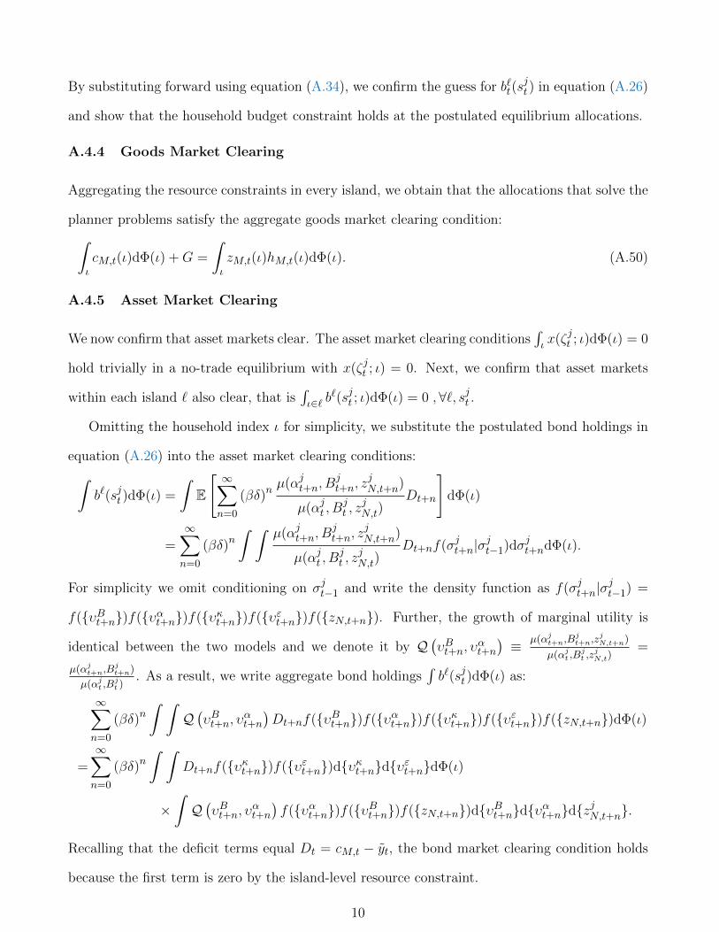
By substituting forward using equation (A.34), we confirm the guess for b`t(sjt ) in equation (A.26)

and show that the household budget constraint holds at the postulated equilibrium allocations.

A.4.4 Goods Market Clearing

Aggregating the resource constraints in every island, we obtain that the allocations that solve the

planner problems satisfy the aggregate goods market clearing condition:∫ιcM,t(ι)dΦ(ι) +G =

∫ιzM,t(ι)hM,t(ι)dΦ(ι). (A.50)

A.4.5 Asset Market Clearing

We now confirm that asset markets clear. The asset market clearing conditions∫ι x(ζjt ; ι)dΦ(ι) = 0

hold trivially in a no-trade equilibrium with x(ζjt ; ι) = 0. Next, we confirm that asset markets

within each island ` also clear, that is∫ι∈` b

`(sjt ; ι)dΦ(ι) = 0 ,∀`, sjt .

Omitting the household index ι for simplicity, we substitute the postulated bond holdings in

equation (A.26) into the asset market clearing conditions:∫b`(sjt )dΦ(ι) =

∫E

[ ∞∑n=0

(βδ)nµ(αjt+n, B

jt+n, z

jN,t+n)

µ(αjt , Bjt , z

jN,t)

Dt+n

]dΦ(ι)

=

∞∑n=0

(βδ)n∫ ∫

µ(αjt+n, Bjt+n, z

jN,t+n)

µ(αjt , Bjt , z

jN,t)

Dt+nf(σjt+n|σjt−1)dσ

jt+ndΦ(ι).

For simplicity we omit conditioning on σjt−1 and write the density function as f(σjt+n|σjt−1) =

f({υBt+n})f({υαt+n})f({υκt+n})f({υεt+n})f({zN,t+n}). Further, the growth of marginal utility is

identical between the two models and we denote it by Q(υBt+n, υ

αt+n

)≡ µ(αjt+n,B

jt+n,z

jN,t+n)

µ(αjt ,Bjt ,z

jN,t)

=

µ(αjt+n,Bjt+n)

µ(αjt ,Bjt )

. As a result, we write aggregate bond holdings∫b`(sjt )dΦ(ι) as:

∞∑n=0

(βδ)n∫ ∫

Q(υBt+n, υ

αt+n

)Dt+nf({υBt+n})f({υαt+n})f({υκt+n})f({υεt+n})f({zN,t+n})dΦ(ι)

=

∞∑n=0

(βδ)n∫ ∫

Dt+nf({υκt+n})f({υεt+n})d{υκt+n}d{υεt+n}dΦ(ι)

×∫Q(υBt+n, υ

αt+n

)f({υαt+n})f({υBt+n})f({zN,t+n})d{υBt+n}d{υαt+n}d{z

jN,t+n}.

Recalling that the deficit terms equal Dt = cM,t − yt, the bond market clearing condition holds

because the first term is zero by the island-level resource constraint.

10

B Observational Equivalence Theorem

In this appendix we derive the identified sources of heterogeneity {αt, εt, Bt}ι presented in Table 2.

Our strategy is to invert the equilibrium allocations presented in Table 1 and solve for the unique

sources of heterogeneity that lead to these allocations. We note that the identification is defined

up to a constant because the constant C that appears in the equations of Table 2 depends on the

ε’s.

B.1 No Home Production, ω = 1

Given cross-sectional data {cM,t, hM,t, zM,t}ι and parameters γ, η, τ0, τ1, we show that there exists

a unique {αt, εt, Bt}ι such that the equilibrium allocations generated by the model are equal to

the data for every household ι. We divide market consumption with home hours to obtain:

cM,t

hM,t= (1− τ0) z−η(1−τ1)M,t exp((1− τ1)(1 + η)αt)

∫ζt

exp((1− τ1)(1 + η)εt)dΦζjt(ζjt ) . (A.51)

Since the left-hand side is a positive constant and the right-hand is increasing in αt, the value

of αt is determined uniquely for every household ι from this equation. Since log zM,t = αt + εt,

the εt is also uniquely determined. Finally, we can use the solution for cM,t or hM,t in Table 1 to

solve for a unique value of Bt.

B.2 Home Production, ω < 1

Given cross-sectional data {cM,t, hM,t, zM,t, hN,t}ι and parameters ω, φ, γ, η, τ0, τ1, we show that

there exists a unique {αt, εt, Bt, zN,t}ι such that the equilibrium allocations generated by the

model are equal to the data for every household ι. We divide the equilibrium allocation of home

hours by market consumption to obtain:

zM,thN,tcM,t

=

(1− ωω

)φ( zjN,tzjM,t

)φ−1. (A.52)

Next, we divide total hours by market consumption, and use (A.52), to obtain:

hM,t + hN,tcM,t

=zη(1−τ1)M,t

1− τ0exp(−(1 + η)(1− τ1)αjt )

(1 + (1− τ0)zM,t

1−τ1 hN,tcM,t

)∫Zt

exp((1 + η)(1− τ1)εt)dΦζj ,t(ζjt ). (A.53)

11

Since the left-hand side is a positive constant and the right-hand is increasing in αt, the value of

αt is determined uniquely for every household ι from this equation. Since log zM,t = αt + εt, the

εt is also uniquely determined. Using equation (A.52), we next obtain a unique value for zN,t.

Finally, we can use the solution for cM,t, hM,t, or hN,t in Table 1 to solve for a unique value of

Bt.

C Description of Data Sources

In this appendix we describe the data sources and the sample construction in more detail.

C.1 Consumer Expenditure Survey

We integrate information from surveys conducted between 1996 and 2016. For each quarter, we

combine the family data (FMLI), which provide household expenditures, with the member data

(MEMI), which contain individual income. Surveys that have been conducted in the first quarter

of year t may be recorded in year t as well as year t−1. The two records are not always identical.

When a survey is recorded twice, we use the last recorded information for each variable. We

merge the information collected across the quarterly surveys to obtain annual data. We allocate

each household to the calendar year for which most of its recorded surveys apply.

We deflate food and alcoholic beverages with its deflator and all other spending categories using

the consumer price index. For our baseline analyses, our definition of non-durable consumption

expenditures includes (i) food and alcoholic beverages, (ii) tobacco and smoking supplies, (iii)

personal care, (iv) utilities, fuels, and public services, (v) household operations (which includes

child care), (vi) public and other transportation, (vii) gasoline and motor oil, (viii) apparel and

services, (ix) reading materials, as well as (x) miscellaneous items.

C.2 American Time Use Survey

We use the ATUS waves between 2003 and 2016. Our definition of time spent on home production

is identical to Aguiar, Hurst, and Karabarbounis (2013) and includes activities such as cooking,

child care, gardening, shopping, caring for others, as well as home, garden, and car maintenance.

12

We merge the information on time use with background characteristics of the respondents using

the additional CPS, roster, and respondent files in the ATUS. These files provide data on variables

such as age, sex, race, education, labor force status, earnings, hours worked, number of children,

and the age of the youngest child. We use this information to obtain a large set of shared

individual characteristics between the ATUS and CEX. We use this set of common characteristics

to impute information from the ATUS into the CEX.

C.3 Sample Adjustment and Imputation

In our baseline specification, we focus on married and cohabiting households with a household

head that is between age 25 and age 65, excluding students. We restrict the sample to households

that have completed all four CEX interviews. We exclude outliers in terms of food consumption,

non-durable consumption, and total spending (bottom and top 1 percent), in terms of market

hours (above 92 hours per week), and in terms of wages (below 3 dollars or above 300 dollars).

To impute home hours from the ATUS into the CEX we use an iterative procedure based on

mean hours conditional on group characteristics. To do so, we construct four groups of variables:

1. Work status, race, gender, age.

2. All previous and cohort, family status, and education.

3. All previous and disability status, retirement status, and geographic information.

4. All previous and hours and wage conditional on working.

For every individual in the CEX, we first evaluate at the finest (fourth) level whether there exist

individuals in the ATUS that share the same group characteristics. When such individuals exist

in the ATUS, we impute the mean of their home hours to the individual in the CEX. If such a

group does not exist, we move to a more coarse level (third), and so on. We repeat this procedure

for each observation in the CEX. Applying this procedure, we account for approximately three

quarters of the variation in home hours. To ensure that our imputation does not introduce

spurious correlations in the merged CEX/ATUS data, we have confirmed that the correlation of

home hours with market hours and wages conditional on age is similar between the ATUS sample

and the merged CEX/ATUS sample.

13

C.4 Longitudinal Internet Studies for the Social Sciences

The Longitudinal Internet Studies for the Social Sciences (LISS) panel is administered by Cen-

tERdata in the Netherlands. The panel is based on a representative sample of Dutch households

who participate in monthly surveys. We use the three waves of this panel (2009, 2010, and 2012)

that contain information on time use.

We define home production time as close as possible to the ATUS. Specifically, home pro-

duction time includes household chores, child care, and administrative chores. Market hours are

measured by time spent on paid work, which includes commuting time. Consumption expendi-

tures include food, utilities, home maintenance, transportation, daycare, and child support. Our

findings are robust to broader and narrower definitions of consumption expenditures.

As in our analysis for the United States, we consider married and cohabiting households with

a head between 25 and 65 years of age that completed both the time use and the consumption

expenditure survey. We drop outliers in terms of total expenditures, non-durable consumption,

and hours worked. Our final sample contains 1,242 observations.

C.5 Japanese Panel Survey of Consumers

The Japanese Panel Survey of Consumers (JPSC) covers the periods between 1998 and 2014.

The JPSC records information for time use on workdays as well as on days off. The dataset

includes time spent on commuting, working, studying, home production and child care, leisure,

and sleeping, personal care and eating. For home hours we use the variable for home production

and child care and for market hours we use the hours worked. To calculate the home and market

hours for a given week, we weight the time use on workdays and days off by the number of days

worked. Our measure of consumption expenditures includes food, utilities, apparel, transport,

culture and leisure, communication, trips and activities, house and land rent. Our findings are

robust to broader and narrower definitions of consumption expenditures.

We focus on married households with complete information on time use as well as expenditures.

We restrict the sample to households with a head between age 25 and age 60 to avoid having less

than 40 observations per age group. This leaves us with 14,548 observations for 2,225 households.

14