infinitely repeated games with discounting page 1...

Infinitely Repeated Games with Discounting

[email protected] Jim Ratliff virtualperfection.com/gametheory

Infinitely Repeated Games with DiscountingÙ

Introduction ______________________________________________________________________1Discounting the future______________________________________________________________2

Interpreting the discount factor______________________________________________________3The average discounted payoff ______________________________________________________4

Restricting strategies to subgames ____________________________________________________7Appendix: Discounting Payoffs______________________________________________________10

In a hurry? ____________________________________________________________________10The infinite summation of the discount factors ________________________________________10An infinite summation starting late__________________________________________________11The finite summation ____________________________________________________________12Endless possibilities ______________________________________________________________13

Introduction

We’ll now discuss repeated games which are “infinitely repeated.” This need not mean that the gamenever ends, however. We will see that this framework is appropriate for modeling situations in which thegame eventually ends (with probability one) but the players are uncertain about exactly when the lastperiod is (and they always believe there’s some chance the game will continue to the next period).

We’ll call the stage game G and interpret it to be a simultaneous-move matrix game which remainsexactly the same through time. As usual we let the player set be I={1,…,n}. Each player has a pureaction space Ai.1 The space of action profiles is A=X i˙IÙAi. Each player has a von Neumann-Morgenstern utility function defined over the outcomes of G, gi:ÙA§Â.

The stage game repeats each period, starting at t=0. Although each stage game is a simultaneous-move game, so that each player acts in ignorance of what her opponent is doing that period, we make the“observable action” or “standard signaling” assumption that the play which occurs in each repetition ofthe stage game is revealed to all the players before the next repetition. Combined with perfect recall, thisallows a player to condition her current action on all earlier actions of her opponents.

We can think of the players as receiving their stage-game payoffs period-by-period. Their repeated-game payoffs will be an additively separable function of these stage-game payoffs. Right away we see apotential problem: There is an infinite number of periods and, hence, of stage-game payoffs to be added

Ù Û © 1996 by Jim Ratliff , <[email protected]>, <http://virtualperfection.com/gametheory>.1 I want to reserve “s” and “S” to represent typical strategies and strategy spaces, respectively, in the repeated game. So I’m using “a” and

“A” for stage-game actions and action spaces.



up. In order that the players’ repeated-game payoffs be well defined we must ensure that this infinitesum does not blow up to infinity. We ensure the finiteness of the repeated-game payoffs by introducingdiscounting of future payoffs relative to earlier payoffs. Such discounting can be an expression of timepreference and/or uncertainty about the length of the game. We introduce the average discounted payoffas a convenience which normalizes the repeated-game payoffs to be “on the same scale” as the stage-game payoffs.

Infinite repetition can be key to obtaining behavior in the stage games which could not be equilibriumbehavior if the game were played once or a known finite number of times. For example, finking everyperiod by both players is the unique equilibrium in any finite repetition of the prisoners’ dilemma.2

When repeated an infinite number of times, however, cooperation in every period is an equilibrium if theplayers are “sufficiently patient.”

We first show that cooperation is a Nash equilibrium of the infinitely repeated game for sufficientlypatient players. Then we discuss subgames of infinitely repeated games and show that, in our uniformlydiscounted payoff scenario, a subgame is the same infinitely repeated game as the original game. Wederive how to restrict a repeated-game strategy to a subgame. This allows us to complete the analysis ofthe example by showing that cooperation in every period by both players is a subgame-perfectequilibrium of the infinitely repeated prisoners’ dilemma for sufficiently patient players.

Discounting the future

When we study infinitely repeated games we are concerned about a player who receives a payoff in eachof infinitely many periods. In order to represent her preferences over various infinite payoff streams wewant to meaningfully summarize the desirability of such a sequence of payoffs by a single number. Acommon assumption is that the player wants to maximize a weighted sum of her per-period payoffs,where she weights later periods less than earlier periods.

For simplicity this assumption often takes the particular form that the sequence of weights forms ageometric progression: for some fixed ∂˙(0,1), each weighting factor is ∂ times the previous weight. (∂is called her discount factor.) If in each period t player i receives the payoff ui

t, we could summarize thedesirability of the payoff stream ui

0, ui1,… by the number3,4

∂tuit∑

t›0

∞

. (1)

Such an intertemporal preference structure has the desirable property that the infinite sum of the

2 See Theorem 4 of “Repeated Games.”3 It’s imperative that you not confuse superscripts with exponents! You should be able to tell from context. For example, in the

summation (1), the t in “∂t” is an exponent; in xit, it is a superscript identifying the time period.

4 Note that this assigns a weight of unity to period zero. It’s the relative weights which are important (why?), so we are free to normalizethe weights any way we want.



weighted payoffs will be finite (since the stage-game payoffs are bounded). You would be indifferentbetween a payoff of xt at time t and a payoff of xtÁ† received † periods later if

xt=∂†xtÁ†. (2)

A useful formula for computing the finite and infinite discounted sums we will encounter is

∂t∑t›T1

T2

=∂T1_∂T2Á1

1_∂, (3)

which, in particular, is valid for T2=∞.5

Interpreting the discount factor

One way we can interpret the discount factor ∂ is as an expression of traditional time preference. Forexample, if you received a dollar today you could deposit it in the bank and it would be worth $(1+r)tomorrow, where r is the per-period rate of interest. You would be indifferent between a payment of $xt

today and $xtÁ† received † periods later only if the future values were equal: (1+r)†xt=xt+†. Comparingthis indifference condition with (2), we see that the two representations of intertemporal preference areequivalent when

∂= 11+r

. (4)

We can relate a player’s discount factor ∂ to her patience. How much more does she value a dollartoday, at time t, than a dollar received †>0 periods later? The relative value of the later dollar to theearlier is ∂tÁ†/∂t=∂†. As ∂§1, ∂†§1, so as her discount factor increases she values the later amountmore and more nearly as much as the earlier payment. A person is more patient the less she mindswaiting for something valuable rather than receiving it immediately. So we interpret higher discountfactors as higher levels of patience.

There’s another reason you might discount the future. You may be unsure about how long the gamewill continue. Even in the absence of time preference per se, you would prefer a dollar today rather thana promise of one tomorrow because you’re not sure tomorrow will really come. (A payoff at a futuretime is really a conditional payoff—conditional on the game lasting that long.)

For example, assume that your beliefs about the length of the game can be represented by a constantconditional continuation probability ®; i.e. conditional on time t being reached, the probability that thegame will continue at least until the next period is ®.6 Without loss of generality we assign a probability

5 See the “Appendix: Discounting Payoffs” for a derivation of this formula.6 Note that there is no upper bound which limits the length of the game; for any value of T˙z++, there is a positive probability of the

game lasting more than T periods. If, on the other hand, players’ beliefs about the duration are such that there is a common knowledgeupper bound T on the length of the game, the game is similar to a finitely repeated game with a common knowledge and definite



of one to the event that we reach period zero.7 Denote by pªtº the probability that period t is reached andby p ªt|t’º the probability that period t is reached conditional on period t’ being reached; sop ªt+1|tº=® for all t. The probability of reaching period 1 is pª1º=pª1|0ºpª0º=®æ1=®. Theprobability of reaching period 2 is pª2º=pª2|1ºpª1º=®2. In general, the probability of reaching periodt is pªtº=®t. The probability that the game ends is 1_pª∞º=1, i.e. one minus the probability that itcontinues forever; therefore the game is finitely repeated with probability one.

Consider the prospect of receiving the conditional payoff of one dollar at time t, given your timepreference ∂ and the conditional continuation probability ®. The probability that the payoff will bereceived is the probability that period t is reached, viz. ®t. Its discounted value if received is ∂t and zeroif not received. Therefore its expected value is ®t∂t=∂t , where ∂fi®∂ is the discount factor which isequivalent to the combination of the time preference with continuation uncertainty. So, even though thegame is finitely repeated, due to the uncertainty about its duration we can model it as an infinitelyrepeated game.

The average discounted payoff

If we adopted the summation (1) as our players’ repeated-game utility function, and if a player receivedthe same stage-game payoff vi in every period, her discounted repeated-game payoff, using (3), wouldbe vi/(1_∂). This would be tolerable, but we’ll find it more convenient to transform the repeated-gamepayoffs to be “on the same scale” as the stage-game payoffs, by multiplying the discounted payoff sumfrom (1) by (1_∂). So we define the average discounted value of the payoff stream ui

0, ui1,… by

(1_∂) ∂tuit∑

t›0

∞

. (5)

Now if a player receives the stage-game payoff vi in every period, her repeated-game payoff is vi aswell. What could be simpler?8

Let’s make some sense of why (5) is interpreted as an average payoff. Consider some time varyingsequence of payoffs ut, for t=0,1,2,…, and let V be the resulting value of the payoff function (5). Nowreplace every per-period payoff ut with the value V. The value of the payoff function (5) associated withthis new constant-payoff stream of V,V,V,… is

(1_∂) ∂tV∑t›0

∞

=V(1_∂) ∂t∑t›0

∞

=V.

duration in the following sense: If the stage game has a unique Nash equilibrium payoff vector, every subgame-perfect equilibrium ofthe repeated game involves Nash equilibrium stage-game behavior in every period.

7 If we don’t get to period zero, we never implement our strategies. Therefore we can assume that we have reached period zero if we doindeed implement our strategies.

8 We will see at a later date that an additional advantage to this normalization is that the convex hull of the feasible repeated-gamepayoffs using the average discounted value formulation is invariant to the discount factor.



In other words, the average discounted payoff of a payoff stream u0,u1,u2,… is that value V which, ifyou received it every period, would give you the same average discounted payoff as the original stream.

We’ll often find it convenient to compute the average discounted value of an infinite payoff stream interms of a leading finite sum and the sum of a trailing infinite substream. For example, say that thepayoffs vi

t a player receives are some constant payoff vi’ for the first t periods, viz. 0,1,2,…,t_1, andthereafter she receives a different constant payoff vi” in each period t,t+1,t+2,…. The averagediscounted value of this payoff stream is

(1_∂) ∂†vi†∑

†›0

∞

=(1_∂)Ù ∂†vi†∑

†›0

t¥1

+ ∂†vi†∑

†›t

∞

=(1_∂)Ùvi

‘ 1_∂t

1_∂+

vi“∂t

1_∂= 1_∂t Ùvi

‘+∂tvi“. (6)

We see that the average discounted value of this stream of bivalued stage-game payoffs is a convexcombination of the two stage-game payoffs.

We can iterate this procedure in order to evaluate the average discounted value of more complicatedpayoff streams. For example—and this one will be particularly useful—say you receive vi’ for the tperiods 0,1,…,t_1 as before, and then you receive vi” only in period t and receive viÉ every periodthereafter. The average discounted value of the stream beginning in period t (discounted to period t) is(1_∂)vi”+∂viÉ. Substituting this for vi” in (6), we find that the average discounted value of this three-valued payoff stream is

(1_∂t)vi’+∂t[(1_∂)vi”+∂viÉ]. (7)

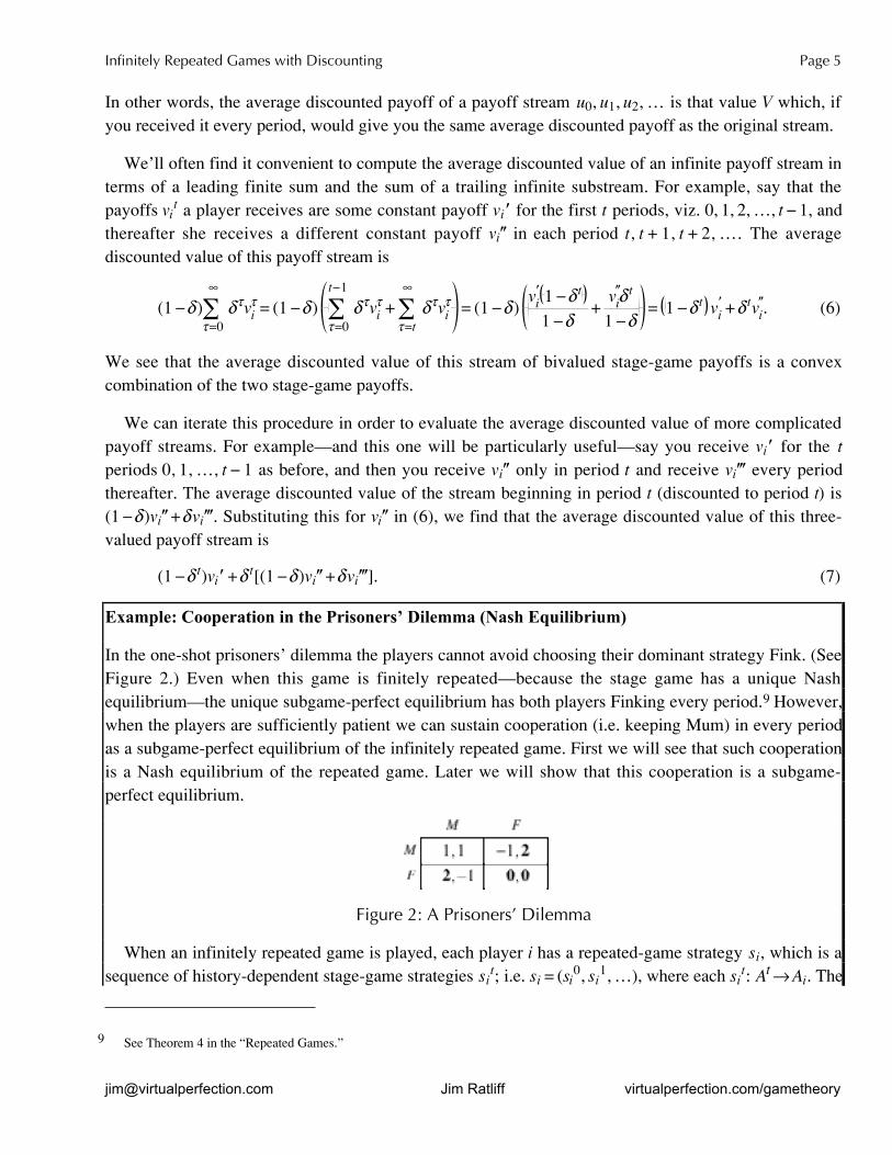
Example: Cooperation in the Prisoners’ Dilemma (Nash Equilibrium)

In the one-shot prisoners’ dilemma the players cannot avoid choosing their dominant strategy Fink. (SeeFigure 2.) Even when this game is finitely repeated—because the stage game has a unique Nashequilibrium—the unique subgame-perfect equilibrium has both players Finking every period.9 However,when the players are sufficiently patient we can sustain cooperation (i.e. keeping Mum) in every periodas a subgame-perfect equilibrium of the infinitely repeated game. First we will see that such cooperationis a Nash equilibrium of the repeated game. Later we will show that this cooperation is a subgame-perfect equilibrium.

Figure 2: A Prisoners’ Dilemma

When an infinitely repeated game is played, each player i has a repeated-game strategy si, which is asequence of history-dependent stage-game strategies si

t; i.e. si=(si0,si

1,…), where each sit:ÙAt§Ai. The

9 See Theorem 4 in the “Repeated Games.”



n-tuple of individual repeated-game strategies is the repeated-game strategy profile s; i.e. s=(s1,…,sn).

The repeated-game strategies I exhibit, which are sufficient to sustain cooperation, have the followingform: Cooperate (i.e. play Mum) in the first period. In later periods, cooperate if both players havealways cooperated. However, if either player has ever Finked, Fink for the remainder of the game. Moreprecisely and formally, we write player i’s repeated-game strategy si=(si

0,si1,…) as the sequence of

history-dependent stage-game strategies such that in period t and after history ht,

(8)

Recall that the history ht is the sequence of stage-game action profiles which were played in the t periods0,1,2,…,t_1. “((M,M)t)” is just a way of writing “((M,M), (M,M),…,(M,M))”, where “(M,M)” isrepeated t times.

We can simplify (8) further in a way that will be useful in our later analysis: Because h0 is the nullhistory, we adopt the convention that, for any action profile a˙A, the statement h0=(a)0 is true.10 Withthis understanding, t=0 implies that ht=((M,M)t). Therefore

(9)

First, I’ll show that for sufficiently patient players the strategy profile s=(s1,s2) is a Nash equilibriumof the repeated game. Later I’ll show that for the same required level of patience these strategies are alsoa subgame-perfect equilibrium.

If both players conform to the alleged equilibrium prescription, they both play Mum at t=0.Therefore at t=1, the history is h1=(M,M); so they both play Mum again. Therefore at t=2, the historyis h2=((M,M),(M,M)), so they both play Mum again. And so on…. So the path of s is the infinitesequence of cooperative action profiles ((M,M),(M,M),…). The repeated-game payoff to each playercorresponding to this path is trivial to calculate: They each receive a payoff of 1 in each period,therefore the average discounted value of each player’s payoff stream is 1.

Can player i gain from deviating from the repeated-game strategy si given that player j is faithfullyfollowing sj? Let t be the period in which player i first deviates. She receives a payoff of 1 in the first tperiods 0,1,…,t_1. In period t, she plays Fink while her conforming opponent played Mum, yieldingplayer i a payoff of 2 in that period. This defection by player i now triggers an open-loop Fink-alwaysresponse from player j. Player i’s best response to this open-loop strategy is to Fink in every period

10 Here is a case of potential ambiguity between time superscripts and exponents. “(a)0” means “a” raised to the zero power; i.e. theprofile a is played zero times.



herself. Thus she receives zero in every period t+1,t+2,…. To calculate the average discounted valueof this payoff stream to player i we can refer to (7), and substitute vi’=1, vi”=2, and viÉ=0. This yieldsplayer i’s repeated-game payoff when she defects in period t in the most advantageous way to be1_∂t(2∂_1). This is weakly less than the equilibrium payoff of 1, for any choice of defection period t,as long as ∂≥™. Thus we have defined what I meant by “sufficiently patient:” cooperation in thisprisoners’ dilemma is a Nash equilibrium of the repeated game as long as ∂≥™.

Restricting strategies to subgames

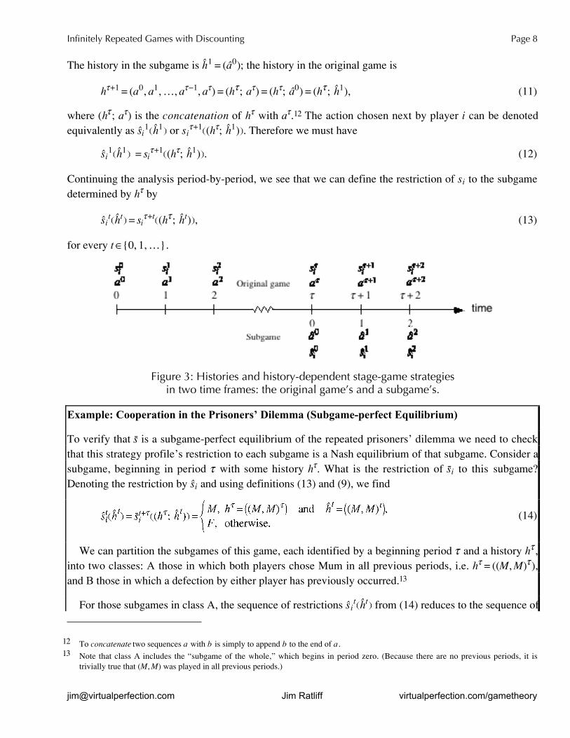
Consider the subgame which begins in period † after a history h†=(a0,a1,…,a†¥1). This subgame isitself an infinitely repeated game; in fact, it is the same infinitely repeated game as the original game inthe sense that 1 the same stage game G is played relentlessly and 2 a unit payoff tomorrow is worth thesame as a payoff of ∂ received today. Another way to appreciate 2 is to consider an infinite stream ofaction profiles a0,a1,…. If a player began in period † to receive the payoffs from this stream of actionprofiles, the contribution to her total repeated-game payoff would be ∂† times its contribution if it werereceived beginning at period zero. If player i were picking a sequence of history-dependent stage-gamestrategies to play beginning when some subgame h† were reached, against fixed choices by heropponents, she would face exactly the same maximization problem as she would if she thought she wasjust starting the game.11

What behavior in the subgame is implied by the repeated-game strategy profile s? The restriction ofthe repeated-game strategy profile s to the subgame h† tells us how the subgame will be played. Let’sdenote this restriction by s. If we played the infinitely-repeated game from the beginning by having eachplayer play her part of s, we would see the same infinite sequence of action profiles as we would see ifinstead s were being played and we began our observation at period †.

For example, in the initial period of the subgame (viz. period † on the original game’s timeline andperiod zero on the subgame’s timeline), player i chooses the action dictated by her subgame strategy si,viz. s i

0. This action must be what her original repeated-game strategy si would tell her to do after thehistory h† by which this subgame was reached. I.e.

si0=si

†ªh†º. (10)

After all the players choose their actions, a stage-game action profile results. We can denote this actionprofile in two ways: as a0, which refers to the initial period of the subgame, or as a†, which refers to thetimeline of the original game. (See Figure 3.) This action profile a0=a† then becomes part of the historywhich conditions the next period’s choices. Period 1 of the subgame is period †+1 of the original game.

11 This paragraph may be unclear, but it’s not a trivial statement! Its validity relies crucially on the structure of the weighting coefficientsin the infinite summation. Let åt be the weight for period t’s per-period payoff. In the discounted payoff case we consider here, we haveåt=∂t. The fact that the “continuation game” is the same game as the whole game is a consequence of the fact that, for all t and †, theratio åtÁ†/åt depends only upon † but not upon t. In our case, this ratio is just ∂†. On the other hand, for example, if the weightingcoefficients were åt=∂t/t, we could not solve each continuation game just as another instance of the original game.



The history in the subgame is h1=(a0); the history in the original game is

h†Á1=(a0,a1,…,a†¥1,a†)=(h†;Ùa†)=(h†;Ùa0)=(h†;Ùh1), (11)

where (h†;Ùa†) is the concatenation of h† with a†.12 The action chosen next by player i can be denotedequivalently as si

1ªh1º or si†Á1ª(h†;Ùh1)º. Therefore we must have

si1ªh1º =si

†Á1ª(h†;Ùh1)º. (12)

Continuing the analysis period-by-period, we see that we can define the restriction of si to the subgamedetermined by h† by

sitªhtº=si

†Átª(h†;Ùht)º, (13)

for every t˙{0,1,…}.

Figure 3: Histories and history-dependent stage-game strategiesin two time frames: the original game’s and a subgame’s.

Example: Cooperation in the Prisoners’ Dilemma (Subgame-perfect Equilibrium)

To verify that s is a subgame-perfect equilibrium of the repeated prisoners’ dilemma we need to checkthat this strategy profile’s restriction to each subgame is a Nash equilibrium of that subgame. Consider asubgame, beginning in period † with some history h†. What is the restriction of si to this subgame?Denoting the restriction by si and using definitions (13) and (9), we find

(14)

We can partition the subgames of this game, each identified by a beginning period † and a history h†,into two classes: A those in which both players chose Mum in all previous periods, i.e. h†=((M,M)†),and B those in which a defection by either player has previously occurred.13

For those subgames in class A, the sequence of restrictions sitªhtº from (14) reduces to the sequence of

12 To concatenate two sequences a with b is simply to append b to the end of a .13 Note that class A includes the “subgame of the whole,” which begins in period zero. (Because there are no previous periods, it is

trivially true that (M,M) was played in all previous periods.)



original stage-game strategies sitªhtº from (9). I.e. for all † and h†=((M,M)†),1415

(15)

Because s is a Nash-equilibrium strategy profile of the repeated game, for each subgame h† in class A ,the restriction s is a Nash-equilibrium strategy profile of the subgame when ∂≥™.

For any subgame h† in class B, h†≠((M,M)†). Therefore the restriction si of s i specifies sit=F for all

t˙{0,1,…}. In other words, in any subgame reached by some player having Finked in the past, eachplayer chooses the open-loop strategy “Fink always.” Therefore the repeated-game strategy profile splayed in such a subgame is an open-loop sequence of stage-game Nash equilibria. From Theorem 1 ofthe Repeated Games handout we know that this is a Nash equilibrium of the repeated game and hence ofthis subgame.

So we have shown that for every subgame the restriction of s to that subgame is a Nash equilibrium ofthat subgame for ∂≥™. Therefore s is a subgame-perfect equilibrium of the infinitely repeated prisoners’dilemma when ∂≥™.

14 When h†=((M,M)†), [h†=((M,M)†) and ht=((M,M)t)] ⁄ ht=((M,M)t).15 There is no distinction between the roles played between ht and ht in these two expressions. They are both dummy variables.



Appendix: Discounting PayoffsOften in economics—for example when we study repeated games—we are concerned about a playerwho receives a payoff in each of many (perhaps infinitely many) periods and we want to meaningfullysummarize her entire sequence of payoffs by a single number. A common assumption is that the playerwants to maximize a weighted sum of her per-period payoffs, where she weights later periods less thanearlier periods. For simplicity this assumption often takes the particular form that the sequence ofweights forms a geometric progression: for some fixed ∂˙(0,1), each weighting factor is ∂ times theprevious weight. (∂ is called her discount factor.) In this handout we’re going to derive some usefulresults relevant to this kind of payoff structure. We’ll see that you really don’t need to memorize abunch of different formulas. You can easily work them all out from scratch from a simple starting point.

Let’s set this problem up more concretely. It will be convenient to call the first period t=0. Let theplayer’s payoff in period t be denoted ut. By convention we attach a weight of 1 to the period 0 payoff.16

The weight for the next period’s payoff, u1, then, is ∂æ1=∂; the weight for the next period’s payoff, u2,then, is ∂æ∂=∂2; the weight for the next period’s payoff, u3, then, is ∂æ∂2=∂3. You see the pattern: ingeneral the weight associated with payoff ut is ∂t. The weighted sum of all the payoffs from t=0§t=T(where T may be ∞) is

u0+∂u1+∂2u2+Ú+∂TuT= ∂tut∑t›0

T. (1)

The infinite summation of the discount factors

We sometimes will be concerned with the case in which the player’s period payoffs are constant oversome stretch of time periods. In this case the common ut value can be brought outside and in front of thesummation over those periods because those ut values don’t depend on the summation index t. Then wewill be essentially concerned with summations of the form

16 It’s the relative weights which are important (why?), so we are free to normalize the sequence of weights any way we want.

In a hurry?

Here’s a formula we’ll eventually derive and from which you can derive a host of other usefuldiscounting expressions. In particular, it’s valid when T2=∞.

∂t∑t›T1

T2

=∂T1_∂T2Á1

1_∂.



∂t∑t=T1

T2

.(2)

To begin our analysis of these summations we’ll first study a special case:

∂t,∑t›0

∞

(3)

and then see how all of the other results we’d like to have can be easily derived from this special case.

The only trick is to see that the infinite sum (3) is mathemagically equal to the reciprocal of (1_∂),i.e.

11Ù–Ù∂

=1+∂+∂2+Ú= ∂t.∑t›0

∞

(4)

To convince yourself that the result of this simple division really is this infinite sum you can use eitherof two heuristic methods. First, there’s synthetic division:17

11_∂1+∂+∂2+Ú

1_∂∂∂_∂2

∂2

∂2_∂3

(5)

If you don’t remember synthetic division from high school algebra, you can alternatively verify (4) bymultiplication:18

(1_∂)(1+∂+∂2+Ú) = (1+∂+∂2+Ú)_∂(1+∂+∂2+Ú)

= (1+∂+∂2+Ú)_(∂+∂2+Ú)

= 1. (6)

An infinite summation starting late

We’ll encounter cases where a player’s per-period payoffs vary in the early periods, say up through

17 I learned this in tenth grade, and I haven’t seen it since; so I can’t give a rigorous justification for it. In particular: its validity in this casemust depend on ∂<1, but I don’t know a precise statement addressing this.

18 Here we rely on ∂<1 to guarantee that the two infinite sums on the right-hand side converge and therefore that we can meaningfullysubtract the second from the first.



period T, but after that she receives a constant payoff per period. To handle this latter constant-payoffstage we’ll want to know the value of the summation

∂t.∑t›TÁ1

∞

(7)

Now that we know the value from (4) for the infinite sum that starts at t=0, we can use that result andthe technique of change of variable in order to find the value of (7).

If only the lower limit on the summation (7) were t=0 instead of t=T+1, we’d know the answerimmediately. So we define a new index †, which depends on t, and transform the summation (7) intoanother summation whose index † runs from 0§∞ and whose summand is ∂†. So, let’s define

†=t_(T+1). (8)

We chose this definition because when t=T+1—like it does for the first term of (7)—then †=0, whichis exactly what we want † to be for the first term of the new summation.19 For purposes of latersubstitution we write (8) in the form

t=†+(T+1). (9)

Substituting for t using (9), summation (7) can now be rewritten as

∂t∑t›TÁ1

∞

= ∂†Á(TÁ1)∑†Á(TÁ1)›TÁ1

∞

=∂TÁ1 ∂†∑†Ù=Ù0

∞

= ∂TÁ1

1 – ∂. (10)

where we used (4) to transform the final infinite sum into its simple reciprocal equivalent.20

The finite summation

Our game might only last a finite number of periods. In this case we want to know the value of

∂t.∑t›0

T(11)

We can immediately get this answer by combining the two results—(4) and (10)—which we’ve alreadyfound. We need only note that the infinite sum in (3) is the sum of two pieces: 1 the piece we want in(11) and 2 the infinite piece in (7). So we immediately obtain

∂t∑t›0

T= ∂t∑

t›0

∞

_ ∂t∑t›TÁ1

∞

= 11_∂

_∂TÁ1

1_∂=1_∂TÁ1

1_∂. (12)

19 Of course, we could have achieved this goal by defining †=(T+1)_t. But we want † to increase with t, so that when t§∞, we’ll alsohave †§∞.

20 The “t” in (4) is just a dummy variable; (4) is still true if you replace every occurrence of “t” with “†”.



Endless possibilities

The techniques we have used here of employing a change of variable and combining previous results isvery general and can be used to obtain the value of summations of the general form in (2). The particularresults we derived, viz. (10) and (12), are merely illustrative cases.

As an exercise, you should be able to easily combine results we have already found here to show thatthe value of the general summation in (2) is

∂t∑t›T1

T2

=∂T1_∂T2Á1

1_∂. (13)

Note that (13) is valid even when T2=∞, because

∂t∑t›T1

∞

= ∂t∑t›T1

T2

limT2§∞

= ∂T1_∂T2Á1

1_∂lim

T2§∞= ∂T1

1_∂, (14)

where we used the fact that

∂tlimt§∞

=0, (15)

for ∂˙[0,1).

You should verify that, by assigning the appropriate values to T1 and T2 in (13), we can recover all ofour previous results, viz. (4), (10), and (12).

infinitely repeated games with discounting page 1...

Documents