inflation in soviet union

8/13/2019 Inflation in Soviet Union

http://slidepdf.com/reader/full/inflation-in-soviet-union 1/25

University of Warwick institutional repository: http://go.warwick.ac.uk/wrap

This paper is made available online in accordance withpublisher policies. Please scroll down to view the documentitself. Please refer to the repository record for this item and our

policy information available from the repository home page forfurther information.

To see the final version of this paper please visit the publisher’s website.access to the published version may require a subscription.

Author(s): Mark Harrison Article Title: Soviet Industrial Production, 1928 to 1955: Real Growthand Hidden Inflation

Year of publication: 2000

Link to published version: http://dx.doi.org/10.1006/jcec.1999.1626Publisher statement: None

http://go.warwick.ac.uk/wrap

http://go.warwick.ac.uk/wrap



This version: 28 September 1999.

Soviet Industrial Production, 1928 to 1955: Real Growth

and Hidden Inflation*

Mark Harrison**

Department of Economics

University of Warwick

Abstract

The mechanism of hidden inflation in Soviet industrial growth statistics between 1928 and

1950 is described. Hidden inflation arose when new products were substituted for old ones.

Substitution biases in Soviet and Western growth estimates are compared; the extent of

hidden inflation in the Soviet figures is estimated. The view that all Soviet growth series were

exaggerated is qualified; the presumption that the lower a figure, the more reliable it must be,

is overturned. The Moorsteen paradox, hidden inflation in industry as a whole, but none in

machinebuilding where product innovation was most rapid, is explained.

JEL codes: N14, P24

* Published in the Journal of Comparative Economics 28:1 (2000), pp. 134-55.

** Mail: Department of Economics, University of Warwick , Coventry, England CV47AL. Email: [email protected].



2

Soviet Industrial Production, 1928 to 1955:

Real Growth and Hidden Inflation1

It is as if we tried to measure how much a caterpillar grows when it turns into a butterfly.

G. Warren Nutter (1962), p. 111

“The difficult problems posed by quality change and the continuing arrival of new

products have been called the “house–to–house combat of price measurement”

Michael J. Boskin et al. (1996), p. 31

1. Introduction

A reconsideration of hidden inflation in Soviet official statistics is timely for three

reasons. First, the end of the Soviet state triggered an outbreak of reassessments of Soviet

long–run economic performance, but measurement issues generally received only a small

share of the attention.2 There is a consensus that Soviet official claims of real growth were

overstated, and there are many independent alternatives, but which should be preferred? A

presumption is sometimes operated in favor of the lowest available figure; it will be shown

below that this presumption is wrong, and that, in exceptional cases, the Soviet figures did

not mislead significantly or were even understated. Second, the opening of the Soviet

statistical archives has allowed us to confirm how the mechanism of hidden inflation

operated, but without revealing its extent (Harrison, 1998). The latter can be only inferred

from comparison of distorted official real growth series with the independent measuresdeemed to be least distorted. Third, the defects of Soviet index number methodology involve

significant issues of comparative economics; for example, they are intimately related to issues

raised more recently by Robert J. Gordon (1990) on measurement of prices of producer

durables in the United States and by the Boskin Committee’s report on the U.S. Consumer

Price Index (Boskin et al., 1996).

The argument is organized as follows. Soviet real output was measured officially in plan

prices, i.e. the unchanged prices of 1926/27. Part 2 shows how Soviet hidden inflation in plan

prices became an issue for Western scholarly research. Part 3 reviews the methodology for

setting plan prices implemented in Soviet industry between 1928 and 1950, contrasts it with

standard index number concepts, and identifies the relative pricing of new and old products asthe central issue. Part 4 compares the main Western estimates in terms of various biases and

derives rough measures of hidden inflation from the outcome. Part 5 reconciles a paradox.

Part 6 concludes.

2. The role of hidden inflation

Soviet economic power made an important contribution to the Allied victory in World

War II. After the war, evaluating the Soviet Union’s economic performance became a major

activity for Western economists.

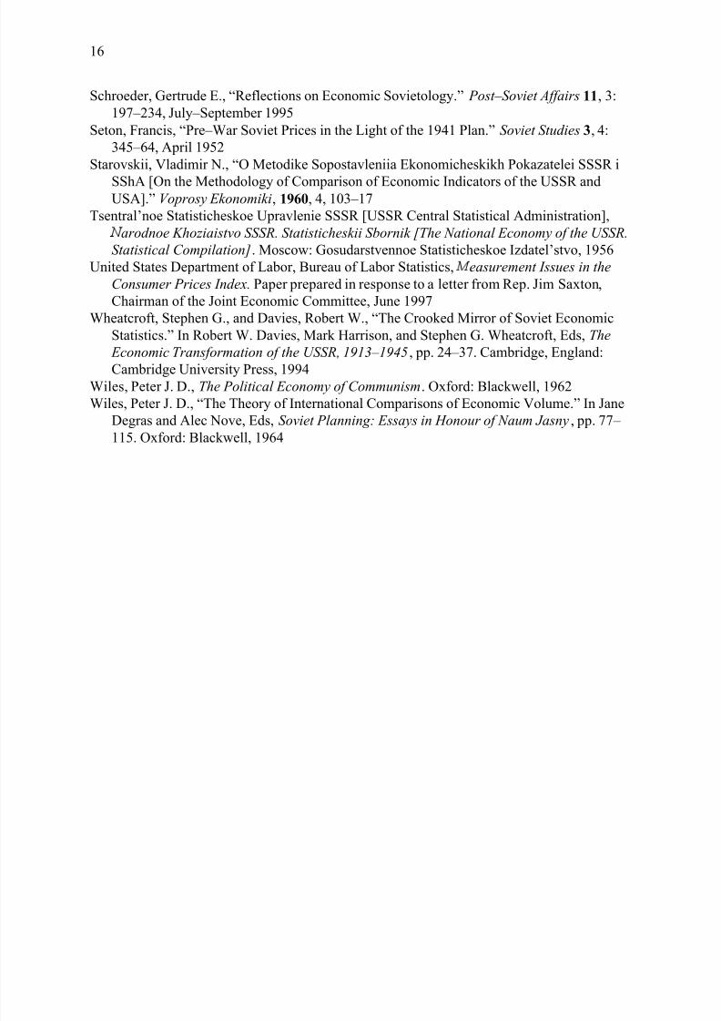
According to the official figures of the Soviet era, between 1928 and 1950, Soviet

national income multiplied by more than 8 times and industrial production by more than 11times in real terms. The underlying series, expressed in plan prices, i.e. the unchanged prices



3

of 1926/27, are shown in Table 1. Western economists agreed that these high official growth

estimates could be only partly justified by true real growth. Several biases were believed to be

at work. There was an upward substitution bias associated with fixed early–year weights in a

Laspeyres–type index, the so–called Gerschenkron effect, which applies when prices and

quantities are negatively correlated.3 Another upward bias arose from the changing coverage

of official statistics; the base–year quantities were unduly low because they excluded smallindustry, which declined thereafter. Various biases, some upward, some downward, resulted

from double–counting intermediate products when adding up the gross value of output

(GVO) leaving each establishment at each stage of production.4 Finally, some of the claimed

growth was believed to reflect hidden inflation.

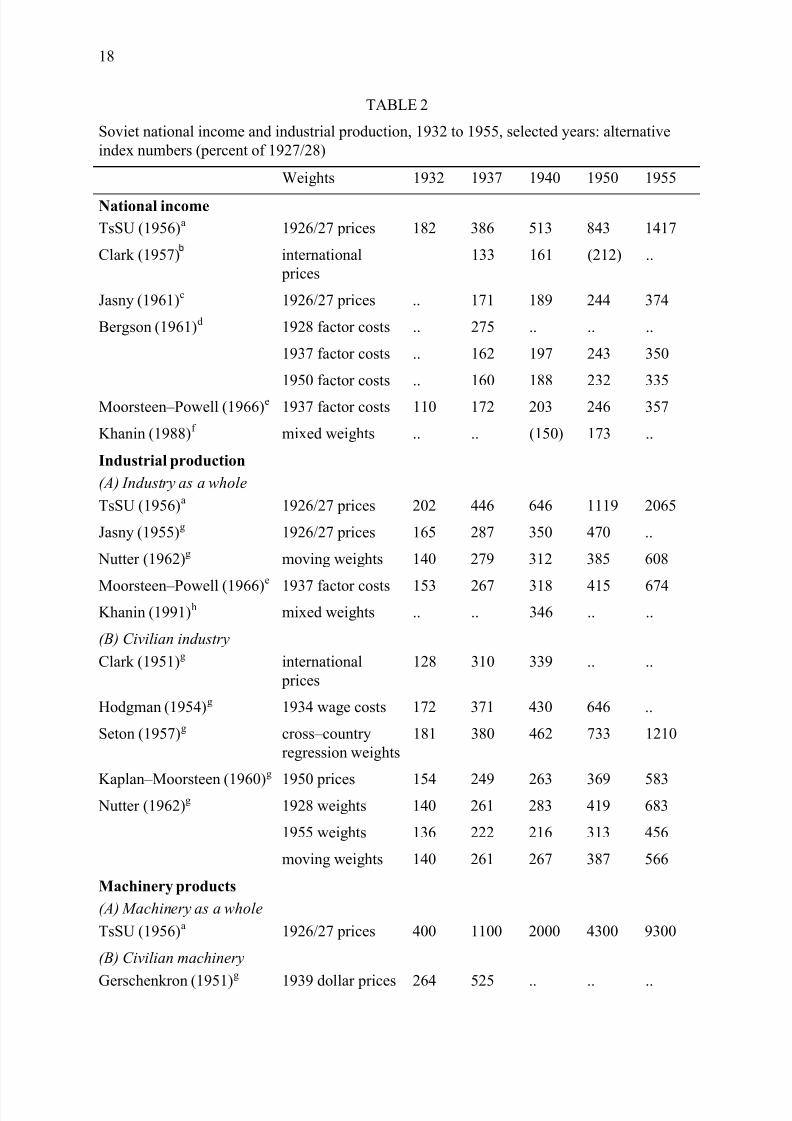
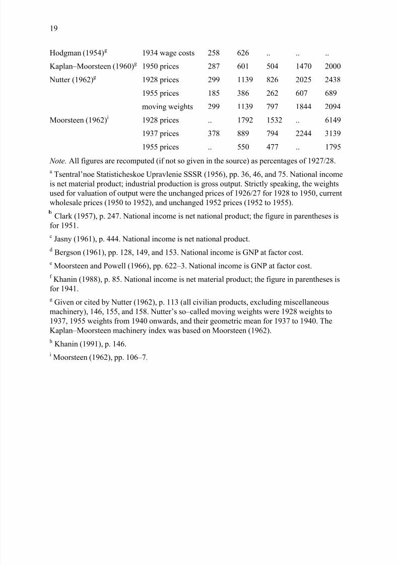
Table 2 compares the main Soviet official and independent evaluations of national

income, industrial production, and machinery production; the more recent figures of Grigorii

Khanin are included for comparison. Admittedly, as the table reveals, the independent

scholars could not agree among themselves. There were many possible solutions to every

problem. Outright disagreements among Western estimates were not uniformly distributed,

being concentrated in the period 1928 to 1937, and in the machinery sector. For other branches and periods the range was narrower. As for aggregate output, in place of the 11–fold

increase in industrial production and 8–fold increase in national income to 1950 claimed

officially, the mainstream Western figures fell in the range of 3 to 7 times and 2 to 3 times

respectively.

Which Western estimates were to be preferred? There was something of a gap between

the studies of the 1950s (Clark, 1951 and 1957, Gerschenkron, 1951, Hodgman, 1954, Jasny,

1955, and Seton, 1957) and those of the 1960s (Kaplan and Moorsteen, 1960, Bergson, 1961,

Nutter, 1962, Moorsteen, 1962, and Moorsteen and Powell, 1966).

The latecomers typically found higher growth rates than the earlier studies, while still

falling far below Soviet official estimates. The earlier studies deployed less complex

methodologies and less abundant data than the later ones. One might expect this to have given

the latecomers the edge, but they were not always favored. Western skeptics such as Peter

Wiles (1962 and 1964) and Alec Nove (1972) distrusted the later attempts to compensate for

the poor quality of data with growing quantity and ever more sophisticated methodology.

More recently a Russian skeptic, Grigorii Khanin (1993), has argued that the less

sophisticated, less informed earlier studies displayed superior economic intuition, and that

their lower real growth estimates ought to be preferred despite their inferior sophistication

and information basis.

Independent estimates diverged, but by less than the gulf between each and the Soviet

official figures. Even allowing for the Soviet preference for an early base year, and despite

varying attempts to correct for other biases, hardly anyone was able to replicate the very high

official figures, although a rare exception, reconsidered below, was Moorsteen on machinery.

The shortfall of the higher Western figures below the Soviet figures was the irreducible

residual which Western scholars attributed to hidden inflation.

Significantly, expert opinion (Clark, 1939, Gerschenkron, 1947, Bergson (1953) rejected

deliberate fabrication as a plausible explanation. Instead of searching for lies, Western

scholars looked for a mechanism of distortion, i.e. a methodology that would lead to

exaggerated real growth estimates without any deliberate intention or special instruction to

lie. They believed they had identified the mechanism in the “unchanged prices ( neizmennye

tseny) of 1926/27” (Gerschenkron, 1947, Dobb, 1948 and 1949, Kaser, 1950, Jasny, 1951a,



4

1951b, and 1952, Seton, 1952, Hodgman, 1954, Nove, 1957, Bergson, 1961, Nutter, 1962,

Moorsteen, 1962).

The unchanged prices of 1926/27 were plan prices that were introduced to assist in

compiling the first five–year plan (1927/28–32) and monitoring its fulfillment by industrial

producers.5 From the outset, statistical and regulatory tasks were intertwined.6 The

institutional environment of a command system with a highly skewed distribution of

information between higher and lower levels encouraged opportunistic behavior by self–

interested producers confronted by ambitious targets set from above. Planners aimed to spur

productive effort, whereas producers aimed to conserve effort while satisfying the plan. The

resources available to planners for monitoring effort were limited. They required simplified

standards against which to measure performance. They fixed a few key targets in physical

units, e.g. tons of oil and coal, kilowatt–hours of electricity. For heterogeneous products, i.e.

machinery, equipment, and consumer goods, planners fixed targets in rubles. However, the

market environment was strongly inflationary; producers leaned towards strategies for

meeting ruble targets that increased prices rather than effort. To limit the scope for fulfilling

the plan through inflation, the planners alighted upon the prices of the year 1926/27 as a fixedstandard of value. Planners fixed GVO quotas and measured results in the unchanged prices

of 1926/27, distributing rewards in proportion to the fulfillment of these quotas.

Product change quickly introduced a fundamental problem: how to form plan prices for

new products on a 1926/27 basis. The years after 1928 saw widespread product innovation in

Soviet industry, especially in machinery where the substitution of home products for imported

machinery rapidly widened the assortment produced. By the mid–1930s the number of

commodities in production which could be matched with the assortment of 1926/27 was

already comparatively small (Rotshtein, 1936).

In the early years, new products would be given plan prices on the basis of either “the

price relating to the initial moment of mass production of the given type of product, or the

average for the first three months of its manufacture” (Rotshtein, 1936, p. 241). This means

that new products were usually valued for plan purposes at the high costs of pilot production

in the early phase of the innovation cycle, when volume was low and the markup for

overheads was high. Once new–product costs began to fall with mass production, the

enterprise could fulfill a given GVO quota made up by new products at high plan prices for

less effort than with old products at low plan prices based on high volume and low unit costs.

The general inflation of the period was a further complication. For example, the GNP

deflator implicit in Bergson’s Soviet national accounts rises from 1928 to 1937 by between 3

times, using 1937 quantity weights, and more than 5 times, using weights of 1928. 7 The effect

of inflation was to raise the initial unit costs of new products above the level which would

have prevailed had the general price level remained stable. Gerschenkron (1947), Jasny

(1951b), and Nutter (1962) argued on this basis that the plan prices of new products were

inflated relative to 1926/27 in two respects: by the high relative costs of pilot production and

also by the rising level of all costs.

3. New and old products in Soviet index numbers

Accounting for product innovation is a central problem for all statistical systems, even in

countries with excellent basic data and huge professional experience. According to Robert

Gordon (1990), as of the 1980s, the United States lacked a good price index for machinery.

Gordon contended that the official series underestimated postwar improvement in the

specifications and performance of producer durables and overstated inflation. The Boskin



5

Commission (Boskin et al., 1996) has similarly criticized the way the US Consumer Price

Index accounts for durables.8

New–product bias is normal in Western statistical methodologies because statisticians are

slow to recognize the substitution of upgraded and new products for existing products.

Eventually new products are chained into the product series as if they are perfect or near

substitutes for old ones. Much growth associated with product innovation is unmeasured;

price changes associated with quality change remained unexplained, except as inflation.9 An

identical bias has been detected in studies of Soviet economic growth that follow a Western

methodology. For example, Michael Boretsky (1987) advanced a parallel critique of Central

Intelligence Agency measures of postwar Soviet industrial prices and production. He charged

CIA analysts with failing to account for growth in new and unique products and upgraded

products, concluding that the associated CIA measures of Soviet inflation were overstated.10

Thus, new–product bias is normal; the new–product bias in Soviet statistics was unusual only

because it carried an opposite sign: it exaggerated real growth, and hid inflation.

The treatment of new products in Soviet index numbers of real output was just one aspect

of an idiosyncratic methodology. Another unusual aspect was that these numbers were based

not on sampling production establishments, outlets, or transactions, but on a comprehensive

count of every single commodity leaving the gates of every factory in the country in every

year. In 1934, for example, more than 39,000 plan prices were approved in Moscow, of which

machinery alone accounted for some 17,000, and the heavy, light, and timber industries

together for more than 28,500 (RGAE, fond 4372, opis’ 23, delo 76, folios 48–50). This was

how new products were included promptly, rather than after the delays characteristic of

Western statistical systems. 11 A further unusual aspect, as will be seen later, was that the

process of aggregation was not divided into upper and lower levels, with sampling of

representative commodities at the lower level and aggregation based on imputed weights at

the upper level. In Soviet practice there were upper and lower levels of aggregation but onlyin a formal, bureaucratic sense. Each product entered a ministerial subtotal before the

subtotals were summed for the gross value of output of industry as a whole. There was no

methodological break between the different levels. Soviet statisticians, e.g. Starovskii (1960),

were proud of their comprehensive coverage, and considered the Western reliance on

sampling and representative commodities to be a methodological flaw.

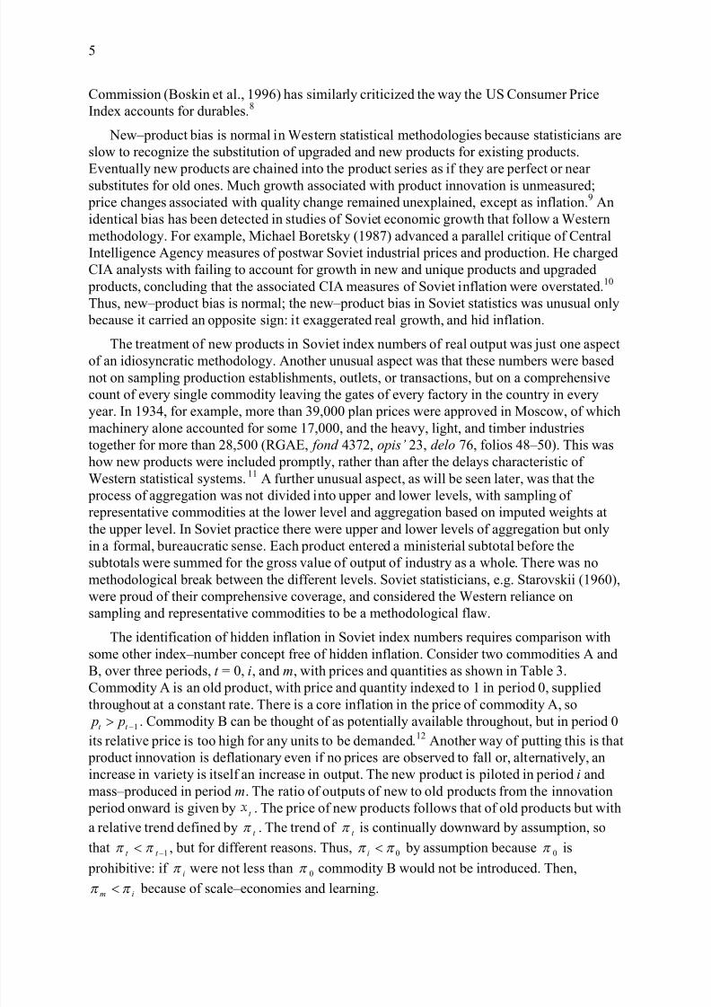
The identification of hidden inflation in Soviet index numbers requires comparison with

some other index–number concept free of hidden inflation. Consider two commodities A and

B, over three periods, t = 0, i, and m, with prices and quantities as shown in Table 3.

Commodity A is an old product, with price and quantity indexed to 1 in period 0, supplied

throughout at a constant rate. There is a core inflation in the price of commodity A, so p pt t 1 . Commodity B can be thought of as potentially available throughout, but in period 0

its relative price is too high for any units to be demanded.12 Another way of putting this is that

product innovation is deflationary even if no prices are observed to fall or, alternatively, an

increase in variety is itself an increase in output. The new product is piloted in period i and

mass–produced in period m. The ratio of outputs of new to old products from the innovation

period onward is given by t . The price of new products follows that of old products but with

a relative trend defined by t . The trend of t is continually downward by assumption, so

that t t 1 , but for different reasons. Thus, 0 i by assumption because 0 is

prohibitive: if i were not less than 0 commodity B would not be introduced. Then,

im because of scale–economies and learning.



6

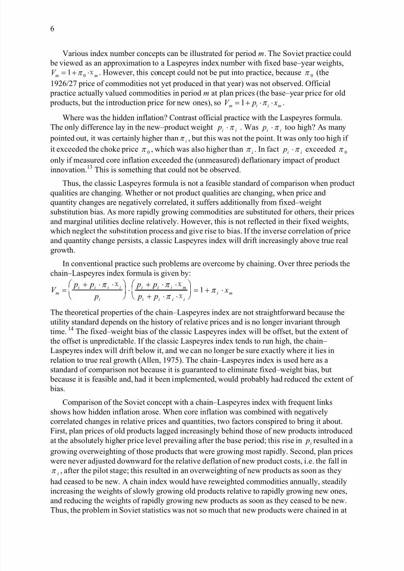
Various index number concepts can be illustrated for period m. The Soviet practice could

be viewed as an approximation to a Laspeyres index number with fixed base–year weights,

V m m 1 0 . However, this concept could not be put into practice, because 0 (the

1926/27 price of commodities not yet produced in that year) was not observed. Official

practice actually valued commodities in period m at plan prices (the base–year price for old

products, but the introduction price for new ones), so V p xm i i m 1 .

Where was the hidden inflation? Contrast official practice with the Laspeyres formula.

The only difference lay in the new–product weight pi i . Was pi i too high? As many

pointed out, it was certainly higher than i , but this was not the point. It was only too high if

it exceeded the choke price 0 , which was also higher than i . In fact pi i exceeded 0

only if measured core inflation exceeded the (unmeasured) deflationary impact of product

innovation.13 This is something that could not be observed.

Thus, the classic Laspeyres formula is not a feasible standard of comparison when product

qualities are changing. Whether or not product qualities are changing, when price and

quantity changes are negatively correlated, it suffers additionally from fixed–weightsubstitution bias. As more rapidly growing commodities are substituted for others, their prices

and marginal utilities decline relatively. However, this is not reflected in their fixed weights,

which neglect the substitution process and give rise to bias. If the inverse correlation of price

and quantity change persists, a classic Laspeyres index will drift increasingly above true real

growth.

In conventional practice such problems are overcome by chaining. Over three periods the

chain–Laspeyres index formula is given by:

V p p

p

p p

p p

xm

i i i i

i

i i i m

i i i i

i m

1

The theoretical properties of the chain–Laspeyres index are not straightforward because the

utility standard depends on the history of relative prices and is no longer invariant through

time. 14 The fixed–weight bias of the classic Laspeyres index will be offset, but the extent of

the offset is unpredictable. If the classic Laspeyres index tends to run high, the chain–

Laspeyres index will drift below it, and we can no longer be sure exactly where it lies in

relation to true real growth (Allen, 1975). The chain–Laspeyres index is used here as a

standard of comparison not because it is guaranteed to eliminate fixed–weight bias, but

because it is feasible and, had it been implemented, would probably had reduced the extent of

bias.

Comparison of the Soviet concept with a chain–Laspeyres index with frequent linksshows how hidden inflation arose. When core inflation was combined with negatively

correlated changes in relative prices and quantities, two factors conspired to bring it about.

First, plan prices of old products lagged increasingly behind those of new products introduced

at the absolutely higher price level prevailing after the base period; this rise in pt resulted in a

growing overweighting of those products that were growing most rapidly. Second, plan prices

were never adjusted downward for the relative deflation of new product costs, i.e. the fall in

t , after the pilot stage; this resulted in an overweighting of new products as soon as they

had ceased to be new. A chain index would have reweighted commodities annually, steadily

increasing the weights of slowly growing old products relative to rapidly growing new ones,

and reducing the weights of rapidly growing new products as soon as they ceased to be new.Thus, the problem in Soviet statistics was not so much that new products were chained in at



7

high introduction prices.15 Rather, old products were never reweighted upwards with inflation

as they became absolutely more expensive, and expensive new products were not reweighted

downwards as they became relatively cheap old products.

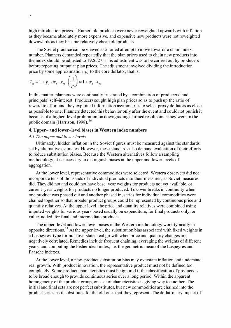
The Soviet practice can be viewed as a failed attempt to move towards a chain index

number. Planners demanded repeatedly that the plan prices used to chain new products into

the index should be adjusted to 1926/27. This adjustment was to be carried out by producers

before reporting output at plan prices. The adjustment involved dividing the introduction

price by some approximation

pi to the core deflator, that is:

V p x p

m i i m

i

i m

1

11

In this matter, planners were continually frustrated by a combination of producers’ and

principals’ self–interest. Producers sought high plan prices so as to push up the ratio of

reward to effort and they exploited information asymmetries to select proxy deflators as close

as possible to one. Planners detected this behavior only after the event and could not punish it

because of a higher–level prohibition on downgrading claimed results once they were in the

public domain (Harrison, 1998).16

4. Upper– and lower–level biases in Western index numbers

4.1 The upper and lower levels

Ultimately, hidden inflation in the Soviet figures must be measured against the standards

set by alternative estimates. However, these standards also demand evaluation of their efforts

to reduce substitution biases. Because the Western alternatives follow a sampling

methodology, it is necessary to distinguish biases at the upper and lower levels of

aggregation.

At the lower level, representative commodities were selected. Western observers did notincorporate tens of thousands of individual products into their measures, as Soviet measures

did. They did not and could not have base–year weights for products not yet available, or

current–year weights for products no longer produced. To cover breaks in continuity when

one product was phased out and another phased in, series for individual commodities were

chained together so that broader product groups could be represented by continuous price and

quantity relatives. At the upper level, the price and quantity relatives were combined using

imputed weights for various years based usually on expenditure, for final products only, or

value–added, for final and intermediate products.

The upper–level and lower–level biases in the Western methodology work typically in

opposite directions.17 At the upper level, the substitution bias associated with fixed weights ina Laspeyres–type formula overstates real growth when price and quantity changes are

negatively correlated. Remedies include frequent chaining, averaging the weights of different

years, and computing the Fisher ideal index, i.e. the geometric mean of the Laspeyres and

Paasche indexes.

At the lower level, a new–product substitution bias may overstate inflation and understate

real growth. With product innovation, the representative product must not be defined too

completely. Some product characteristics must be ignored if the classification of products is

to be broad enough to provide continuous series over a long period. Within the apparent

homogeneity of the product group, one set of characteristics is giving way to another. The

initial and final sets are not perfect substitutes, but new commodities are chained into the product series as if substitutes for the old ones that they represent. The deflationary impact of



8

new or improved characteristics is unmeasured; price changes associated with changes in

characteristics remained unexplained except as inflation. One remedy is to increase the

number of representative products; the more finely defined is the product, the more quality

change is captured in shifts between product groups and the less is lost within them. Others

include the measurement of change in characteristics and of price per unit of each

characteristic, and the prompt incorporation of new products and new characteristics.

Thus there are not only biases at the upper and lower levels but also remedies for these.

Therefore, the independent studies of Western economists may be classified according to the

effectiveness of the particular remedies adopted.

4.2 Lower–level biases

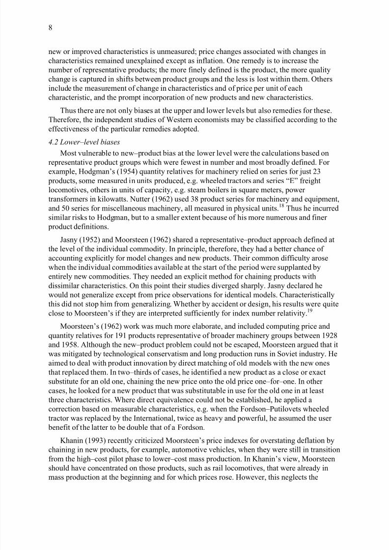
Most vulnerable to new–product bias at the lower level were the calculations based on

representative product groups which were fewest in number and most broadly defined. For

example, Hodgman’s (1954) quantity relatives for machinery relied on series for just 23

products, some measured in units produced, e.g. wheeled tractors and series “E” freight

locomotives, others in units of capacity, e.g. steam boilers in square meters, power transformers in kilowatts. Nutter (1962) used 38 product series for machinery and equipment,

and 50 series for miscellaneous machinery, all measured in physical units.18 Thus he incurred

similar risks to Hodgman, but to a smaller extent because of his more numerous and finer

product definitions.

Jasny (1952) and Moorsteen (1962) shared a representative–product approach defined at

the level of the individual commodity. In principle, therefore, they had a better chance of

accounting explicitly for model changes and new products. Their common difficulty arose

when the individual commodities available at the start of the period were supplanted by

entirely new commodities. They needed an explicit method for chaining products with

dissimilar characteristics. On this point their studies diverged sharply. Jasny declared hewould not generalize except from price observations for identical models. Characteristically

this did not stop him from generalizing. Whether by accident or design, his results were quite

close to Moorsteen’s if they are interpreted sufficiently for index number relativity.19

Moorsteen’s (1962) work was much more elaborate, and included computing price and

quantity relatives for 191 products representative of broader machinery groups between 1928

and 1958. Although the new–product problem could not be escaped, Moorsteen argued that it

was mitigated by technological conservatism and long production runs in Soviet industry. He

aimed to deal with product innovation by direct matching of old models with the new ones

that replaced them. In two–thirds of cases, he identified a new product as a close or exact

substitute for an old one, chaining the new price onto the old price one–for–one. In other

cases, he looked for a new product that was substitutable in use for the old one in at least

three characteristics. Where direct equivalence could not be established, he applied a

correction based on measurable characteristics, e.g. when the Fordson–Putilovets wheeled

tractor was replaced by the International, twice as heavy and powerful, he assumed the user

benefit of the latter to be double that of a Fordson.

Khanin (1993) recently criticized Moorsteen’s price indexes for overstating deflation by

chaining in new products, for example, automotive vehicles, when they were still in transition

from the high–cost pilot phase to lower–cost mass production. In Khanin’s view, Moorsteen

should have concentrated on those products, such as rail locomotives, that were already in

mass production at the beginning and for which prices rose. However, this neglects the



9

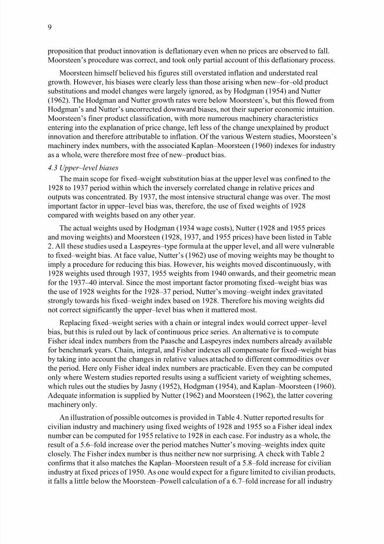
proposition that product innovation is deflationary even when no prices are observed to fall.

Moorsteen’s procedure was correct, and took only partial account of this deflationary process.

Moorsteen himself believed his figures still overstated inflation and understated real

growth. However, his biases were clearly less than those arising when new–for–old product

substitutions and model changes were largely ignored, as by Hodgman (1954) and Nutter

(1962). The Hodgman and Nutter growth rates were below Moorsteen’s, but this flowed from

Hodgman’s and Nutter’s uncorrected downward biases, not their superior economic intuition.

Moorsteen’s finer product classification, with more numerous machinery characteristics

entering into the explanation of price change, left less of the change unexplained by product

innovation and therefore attributable to inflation. Of the various Western studies, Moorsteen’s

machinery index numbers, with the associated Kaplan–Moorsteen (1960) indexes for industry

as a whole, were therefore most free of new–product bias.

4.3 Upper–level biases

The main scope for fixed–weight substitution bias at the upper level was confined to the

1928 to 1937 period within which the inversely correlated change in relative prices andoutputs was concentrated. By 1937, the most intensive structural change was over. The most

important factor in upper–level bias was, therefore, the use of fixed weights of 1928

compared with weights based on any other year.

The actual weights used by Hodgman (1934 wage costs), Nutter (1928 and 1955 prices

and moving weights) and Moorsteen (1928, 1937, and 1955 prices) have been listed in Table

2. All these studies used a Laspeyres–type formula at the upper level, and all were vulnerable

to fixed–weight bias. At face value, Nutter’s (1962) use of moving weights may be thought to

imply a procedure for reducing this bias. However, his weights moved discontinuously, with

1928 weights used through 1937, 1955 weights from 1940 onwards, and their geometric mean

for the 1937–40 interval. Since the most important factor promoting fixed–weight bias wasthe use of 1928 weights for the 1928–37 period, Nutter’s moving–weight index gravitated

strongly towards his fixed–weight index based on 1928. Therefore his moving weights did

not correct significantly the upper–level bias when it mattered most.

Replacing fixed–weight series with a chain or integral index would correct upper–level

bias, but this is ruled out by lack of continuous price series. An alternative is to compute

Fisher ideal index numbers from the Paasche and Laspeyres index numbers already available

for benchmark years. Chain, integral, and Fisher indexes all compensate for fixed–weight bias

by taking into account the changes in relative values attached to different commodities over

the period. Here only Fisher ideal index numbers are practicable. Even they can be computed

only where Western studies reported results using a sufficient variety of weighting schemes,

which rules out the studies by Jasny (1952), Hodgman (1954), and Kaplan–Moorsteen (1960).

Adequate information is supplied by Nutter (1962) and Moorsteen (1962), the latter covering

machinery only.

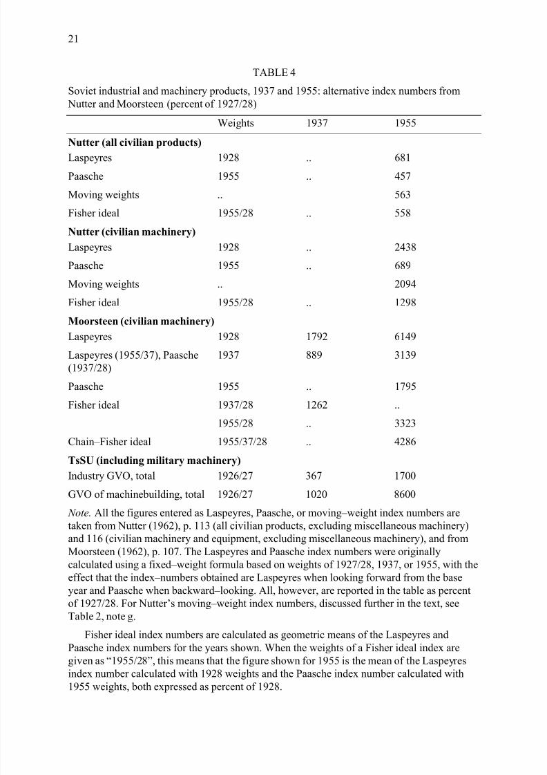
An illustration of possible outcomes is provided in Table 4. Nutter reported results for

civilian industry and machinery using fixed weights of 1928 and 1955 so a Fisher ideal index

number can be computed for 1955 relative to 1928 in each case. For industry as a whole, the

result of a 5.6–fold increase over the period matches Nutter’s moving–weights index quite

closely. The Fisher index number is thus neither new nor surprising. A check with Table 2

confirms that it also matches the Kaplan–Moorsteen result of a 5.8–fold increase for civilian

industry at fixed prices of 1950. As one would expect for a figure limited to civilian products,

it falls a little below the Moorsteen–Powell calculation of a 6.7–fold increase for all industry



10

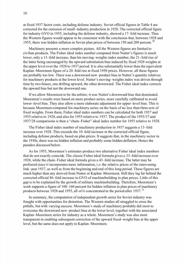
at fixed 1937 factor costs, including defense industry. Soviet official figures in Table 4 are

corrected for the omission of small–industry production in 1928. The corrected official figure

for industry GVO in 1955, including the defense industry, showed a 17–fold increase. Thus

the Western figures would appear to be consistent with the conclusion that, between 1928 and

1955, there was hidden inflation in Soviet plan prices of between 150 and 200 percent.20

Machinery presents a more complex picture. All the Western figures are limited to

civilian products. The Fisher ideal index number computed from Nutter’s figures is much

lower, only a 13–fold increase, than his moving–weights index number, the 21–fold rise of

the latter being encouraged by the upward substitution bias induced by fixed 1928 weights at

the upper level over the 1928 to 1937 period. It is also substantially lower than the equivalent

Kaplan–Moorsteen figure of a 20–fold rise at fixed 1950 prices. However, all these figures

are probably too low. There was a downward new–product bias in Nutter’s quantity relatives

for machinery products at the lower level. Nutter’s moving–weights index was driven through

time by two biases, one drifting upward, the other downward. The Fisher ideal index corrects

the upward bias but not the downward one.

If we allow Moorsteen to be the arbiter, it was Nutter’s downward bias that dominated.

Moorsteen’s results were based on more product series, more carefully calibrated to avoid

lower–level bias. They also allow a more elaborate adjustment for upper–level bias. This is

because Moorsteen computed his machinery series on the basis of no less than three sets of

fixed weights. From them, Fisher ideal index numbers can be calculated for both 1937 and

1955 relative to 1928, and also for 1955 relative to 1937. The product of the 1955/37 and

1937/28 comparisons is then a “chain–Fisher” ideal index number for 1955 relative to 1928.

The Fisher ideal index number of machinery production in 1937 suggests a 13–fold

increase over 1928. This exceeds the 10–fold increase in the corrected official figure,

including defense products, based on plan prices. It suggests that, in the machinery sector in

the 1930s, there was no hidden inflation and probably some hidden deflation. Hence the

paradox discussed below.

As for 1955, Moorsteen’s estimates produce two alternative Fisher ideal index numbers

that do not exactly coincide. The classic Fisher ideal formula gives a 33–fold increase over

1928, while the chain–Fisher ideal formula gives a 43–fold increase. The latter may be

preferred since it incorporates more information, i.e. the relative prices of the intervening

link–year 1937, as well as from the beginning and end of this long period. These figures are

much higher than any derived from Nutter or Kaplan–Moorsteen. Still they lag far behind the

corrected official 86–fold increase in GVO of machinebuilding in plan prices. Little of this

gap is to be explained by the growth of military machinebuilding. Therefore, Moorsteen’s

work supports a figure of 100–160 percent for hidden inflation in plan prices of machinery

products between 1928 and 1955, all of it concentrated in the period after 1937.21

In summary, the computation of independent growth series for Soviet industry was

fraught with opportunities for distortion. The Western studies all struggled to cross the

pitfalls, but with varying success. Moorsteen’s study of machinery probably did most to

overcome the downward new–product bias at the lower level, together with the associated

Kaplan–Moorsteen series for industry as a whole. Moorsteen’s study was also most

transparent in enabling subsequent correction of the upward fixed–weight bias at the upper

level, but the same does not apply to Kaplan–Moorsteen.



11

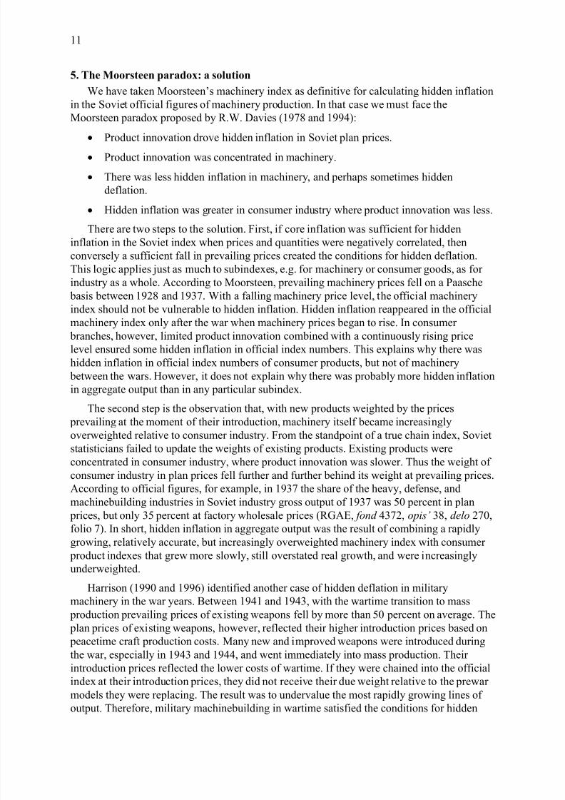
5. The Moorsteen paradox: a solution

We have taken Moorsteen’s machinery index as definitive for calculating hidden inflation

in the Soviet official figures of machinery production. In that case we must face the

Moorsteen paradox proposed by R.W. Davies (1978 and 1994):

Product innovation drove hidden inflation in Soviet plan prices.

Product innovation was concentrated in machinery.

There was less hidden inflation in machinery, and perhaps sometimes hidden

deflation.

Hidden inflation was greater in consumer industry where product innovation was less.

There are two steps to the solution. First, if core inflation was sufficient for hidden

inflation in the Soviet index when prices and quantities were negatively correlated, then

conversely a sufficient fall in prevailing prices created the conditions for hidden deflation.

This logic applies just as much to subindexes, e.g. for machinery or consumer goods, as for

industry as a whole. According to Moorsteen, prevailing machinery prices fell on a Paasche basis between 1928 and 1937. With a falling machinery price level, the official machinery

index should not be vulnerable to hidden inflation. Hidden inflation reappeared in the official

machinery index only after the war when machinery prices began to rise. In consumer

branches, however, limited product innovation combined with a continuously rising price

level ensured some hidden inflation in official index numbers. This explains why there was

hidden inflation in official index numbers of consumer products, but not of machinery

between the wars. However, it does not explain why there was probably more hidden inflation

in aggregate output than in any particular subindex.

The second step is the observation that, with new products weighted by the prices

prevailing at the moment of their introduction, machinery itself became increasinglyoverweighted relative to consumer industry. From the standpoint of a true chain index, Soviet

statisticians failed to update the weights of existing products. Existing products were

concentrated in consumer industry, where product innovation was slower. Thus the weight of

consumer industry in plan prices fell further and further behind its weight at prevailing prices.

According to official figures, for example, in 1937 the share of the heavy, defense, and

machinebuilding industries in Soviet industry gross output of 1937 was 50 percent in plan

prices, but only 35 percent at factory wholesale prices (RGAE, fond 4372, opis’ 38, delo 270,

folio 7). In short, hidden inflation in aggregate output was the result of combining a rapidly

growing, relatively accurate, but increasingly overweighted machinery index with consumer

product indexes that grew more slowly, still overstated real growth, and were increasinglyunderweighted.

Harrison (1990 and 1996) identified another case of hidden deflation in military

machinery in the war years. Between 1941 and 1943, with the wartime transition to mass

production prevailing prices of existing weapons fell by more than 50 percent on average. The

plan prices of existing weapons, however, reflected their higher introduction prices based on

peacetime craft production costs. Many new and improved weapons were introduced during

the war, especially in 1943 and 1944, and went immediately into mass production. Their

introduction prices reflected the lower costs of wartime. If they were chained into the official

index at their introduction prices, they did not receive their due weight relative to the prewar

models they were replacing. The result was to undervalue the most rapidly growing lines of

output. Therefore, military machinebuilding in wartime satisfied the conditions for hidden



12

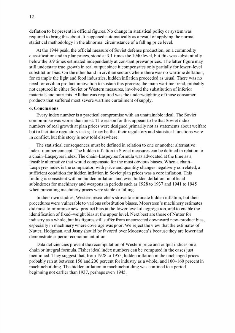
deflation to be present in official figures. No change in statistical policy or system was

required to bring this about. It happened automatically as a result of applying the normal

statistical methodology in the abnormal circumstance of a falling price level.

At the 1944 peak, the official measure of Soviet defense production, on a commodity

classification and in plan prices, stood at 3.1 times the 1940 level, but this was substantially

below the 3.9 times estimated independently at constant prewar prices. The latter figure may

still understate true growth in real output since it compensates only partially for lower–level

substitution bias. On the other hand in civilian sectors where there was no wartime deflation,

for example the light and food industries, hidden inflation proceeded as usual. There was no

need for civilian product innovation to sustain this process; the main wartime trend, probably

not captured in either Soviet or Western measures, involved the substitution of inferior

materials and nutrients. All that was required was the underweighting of those consumer

products that suffered most severe wartime curtailment of supply.

6. Conclusions

Every index number is a practical compromise with an unattainable ideal. The Sovietcompromise was worse than most. The reason for this appears to be that Soviet index

numbers of real growth at plan prices were designed primarily not as statements about welfare

but to facilitate regulatory tasks; it may be that their regulatory and statistical functions were

in conflict, but this story is now told elsewhere.

The statistical consequences must be defined in relation to one or another alternative

index–number concept. The hidden inflation in Soviet measures can be defined in relation to

a chain–Laspeyres index. The chain–Laspeyres formula was advocated at the time as a

feasible alternative that would compensate for the most obvious biases. When a chain–

Laspeyres index is the comparator, with price and quantity changes negatively correlated, a

sufficient condition for hidden inflation in Soviet plan prices was a core inflation. Thisfinding is consistent with no hidden inflation, and even hidden deflation, in official

subindexes for machinery and weapons in periods such as 1928 to 1937 and 1941 to 1945

when prevailing machinery prices were stable or falling.

In their own studies, Western researchers strove to eliminate hidden inflation, but their

procedures were vulnerable to various substitution biases. Moorsteen’s machinery estimates

did most to minimize new–product bias at the lower level of aggregation, and to enable the

identification of fixed–weight bias at the upper level. Next best are those of Nutter for

industry as a whole, but his figures still suffer from uncorrected downward new–product bias,

especially in machinery where coverage was poor. We reject the view that the estimates of

Nutter, Hodgman, and Jasny should be favored over Moorsteen’s because they are lower and

demonstrate superior economic intuition.

Data deficiencies prevent the recomputation of Western price and output indices on a

chain or integral formula. Fisher ideal index numbers can be computed in the cases just

mentioned. They suggest that, from 1928 to 1955, hidden inflation in the unchanged prices

probably ran at between 150 and 200 percent for industry as a whole, and 100–160 percent in

machinebuilding. The hidden inflation in machinebuilding was confined to a period

beginning not earlier than 1937, perhaps even 1945.



13

Appendix: nomenclature

i the innovation period for commodity B

m the mass production period for commodity B

n a period of extended mass production for commodity B

t p the price of commodity A relative to the initial period when t = 0; the core deflator

t p

an approximation to the core deflator

t the price of commodity B relative to that of A

t time

t V a Laspeyres index number

t the output of commodity B relative to that of A



14

References

Abraham, Katherine G., Greenlees, John S., and Moulton, Brent R., “Working to Improve the

Consumer Price Index.” Journal of Economic Perspectives 12, 1: 27–36, Winter 1998

Allen, Roy G. D., Index Numbers in Theory and Practice. Basingstoke: Macmillan, 1975

Becker, Abraham S., “Intelligence Fiasco or Reasoned Accounting?: CIA Estimates of Soviet

GNP.” Post–Soviet Affairs 10, 4: 291–329, October–December 1994

Bergson, Abram, Soviet National Income and Product in 1937. New York: Columbia

University Press, 1953

Bergson, Abram, The Real National Income of Soviet Russia Since 1928. Cambridge, MA:

Harvard University Press, 1961

Boretsky, Michael, “The tenability of the CIA estimates of Soviet economic growth.” Journal

of Comparative Economics 11, 4: 517–42, December 1987

Boretsky, Michael, “CIA’s Queries about Boretsky’s Criticism of its Estimates of Soviet

Economic Growth.” Journal of Comparative Economics 14, 2: 315–26, June 1990

Boskin, Michael J., Dulberger, Ellen R., Gordon, Robert J., Griliches, Zvi, and Jorgensen,

Dale W., Towards a More Accurate Measure of the Cost Of Living . Final Report to theSenate Finance Committee from the Advisory Commission to Study the Consumer Price

Index, December 4, 1996

Boskin, Michael J., Dulberger, Ellen R., Gordon, Robert J., Griliches, Zvi, and Jorgensen,

Dale W., “Consumer Prices, the Consumer Price Index, and the Cost of Living.” Journal

of Economic Perspectives 12, 1: 3–26, Winter 1998

Central Intelligence Agency, An Analysis of the Behavior of Soviet Machinery Prices, 1960–

1973. Washington, DC: National Foreign Assessment Center, Research Paper ER79–

10631, 1979

Clark, Colin (1939), A Critique of Russian Statistics. London: Macmillan

Clark, Colin (1957), The Conditions of Economic Progress, 3rd edn. London: Macmillan

Davies, Robert W., “Soviet Industrial Production, 1928–1937: the Rival Estimates.”

University of Birmingham, Centre for Russian and East European Studies, Soviet

Industrialisation Project Series no. 18, 1978

Davies, Robert W., “Industry.” In Robert W. Davies, Mark Harrison, and Stephen G.

Wheatcroft, Eds, The Economic Transformation of the USSR, 1913–1945, pp. 131–57.

Cambridge, England: Cambridge University Press, 1994

Deaton, Angus, “Getting Prices Right: What Should be Done?” Journal of Economic

Perspectives 12, 1: 37–46, Winter 1998

Diewart, W. Erwin (1987), “Index Numbers.” In John Eatwell, Murray Milgate, and Peter

Newman, Eds, The New Palgrave Dictionary of Economics 2, pp. 767–79. Basingstoke

and London: Macmillan, 1987Dobb, Maurice, “Further Appraisals of Russian Economic Statistics.” Review of Economics

and Statistics 30, 1: 34–8, February 1948

Dobb, Maurice, “Comment on Soviet Economic Statistics.” Soviet Studies 1, 1: 18–27, June

1949

Gerschenkron, Alexander, “The Soviet Indices of Industrial Production.” Review of

Economics and Statistics 29, 4: 217–26, November 1947

Gordon, Robert J., The Measurement of Durable Goods Prices. Chicago, IL, and London:

National Bureau of Economic Research, 1990

Griliches, Zvi, “Hedonic Price Indexes for Automobiles: an Econometric Analysis of Quality

Change.” In National Bureau of Economic Research, The Price Statistics of the Federal



15

Government , pp. 173–96. New York: National Bureau of Economic Research, General

Series no. 3, 1961

Harrison, Mark, “The Volume of Soviet Munitions Output, 1937–1945: a Reevaluation.”

Journal of Economic History 50, 3: 569–89, September 1990

Harrison, Mark, Accounting for War: Soviet Production, Employment, and the Defence

Burden, 1940–1945. Cambridge, England: Cambridge University Press, 1996Harrison, Mark, “Prices, Planners, and Producers: an Agency Problem in Soviet Industry,

1928–1950.” Journal of Economic History 58, 4: 1032–62, December 1998

Hicks, John R., “The Valuation of the Social Income”, Economica 7, 26: 105–24, May 1940

Hodgman, Donald R., Soviet Industrial Production, 1928–1951. Cambridge, MA: Harvard

University Press, 1954

Jasny, Naum, The Soviet Economy During the Plan Era. Stanford, CA: Stanford University,

Food Research Institute, 1951a

Jasny, Naum, The Soviet Price System. Stanford, CA: Stanford University, Food Research

Institute, 1951b

Jasny, Naum, Soviet Prices of Producers’ Goods. Stanford, CA: Stanford University, FoodResearch Institute, 1952

Jasny, Naum, Soviet Industrialization, 1928–1952. Chicago, IL: University of Chicago Press,

1961

Kaplan, Norman M., and Moorsteen, Richard, “Indexes of Soviet Industrial Output”, 2 vols.

Santa Monica, CA: The RAND Corporation, Research Memorandum RM–2495, 1960

Kaser, Michael, “Soviet Planning and the Price Mechanism.” Economic Journal 60, 237: 81–

91, March 1950

Khanin, Grigorii I., “Ekonomicheskii Rost: Al’ternativnaia Otsenka [Economic Growth: an

Alternative Assessment].” Kommunist 1988, 17: 83–90

Khanin, Grigorii I., Dinamika Ekonomicheskogo Razvitiia SSSR [The Dynamics of

Economic Development of the USSR]. Novosibirsk: Nauka, 1991Khanin, Grigorii I., Sovetskii Ekonomicheskii Rost: Analiz Zapadnykh Otsenok [Soviet

Economic Growth: an Analysis of Western Assessments]. Novosibirsk: EKOR, 1993

Kudrov, Valentin M., Sovetskaia Ekonomika v Retrospektive: Opyt Pereosmyslenii [The

Soviet Economic System in Retrospect: an Experiment in Rethinking]. Moscow: Nauka,

1997

Maddison, Angus, “Measuring the Performance of a Communist Command Economy: an

Assessment of the CIA Estimates for the U.S.S.R.” Review of Income and Wealth 44, 3:

307–23, September 1998

Moorsteen, Richard, Prices and Production of Machinery in the Soviet Union, 1928–1958.

Cambridge, MA: Harvard University Press, 1962Moorsteen, Richard, and Powell, Raymond P., The Soviet Capital Stock, 1928–1962.

Homewood, IL: Irwin, 1966

Nove, Alec, “‘1926/7’ and All That.” Soviet Studies 9, 2: 117–30, October 1957

Nove, Alec, An Economic History of the USSR, 1st edn. Harmondsworth: Penguin, 1972

Nutter, G. Warren., The Growth of Industrial Production in the Soviet Union. Princeton, NJ:

National Bureau of Economic Research, 1962

Pitzer, John S., “The Tenability of the CIA Estimates of Soviet Economic Growth: a

Comment.” Journal of Comparative Economics 14, 2: 301–14, June 1990

Rossiiskii Gosudarstvennyi Arkhiv Ekonomiki [Russian State Economics Archive], Moscow

Rotshtein, Aleksandr I., Problemy Promyshlennoi Statistiki SSSR [Problems of Industrial

Statistics of the USSR] 1. Leningrad: Gosudarstvennoe Sotsial’no–Ekonomicheskoe

Izdatel’stvo, 1936



16

Schroeder, Gertrude E., “Reflections on Economic Sovietology.” Post–Soviet Affairs 11, 3:

197–234, July–September 1995

Seton, Francis, “Pre–War Soviet Prices in the Light of the 1941 Plan.” Soviet Studies 3, 4:

345–64, April 1952

Starovskii, Vladimir N., “O Metodike Sopostavleniia Ekonomicheskikh Pokazatelei SSSR i

SShA [On the Methodology of Comparison of Economic Indicators of the USSR andUSA].” Voprosy Ekonomiki, 1960, 4, 103–17

Tsentral’noe Statisticheskoe Upravlenie SSSR [USSR Central Statistical Administration],

arodnoe Khoziaistvo SSSR. Statisticheskii Sbornik [The National Economy of the USSR.

Statistical Compilation]. Moscow: Gosudarstvennoe Statisticheskoe Izdatel’stvo, 1956

United States Department of Labor, Bureau of Labor Statistics, easurement Issues in the

Consumer Prices Index. Paper prepared in response to a letter from Rep. Jim Saxton,

Chairman of the Joint Economic Committee, June 1997

Wheatcroft, Stephen G., and Davies, Robert W., “The Crooked Mirror of Soviet Economic

Statistics.” In Robert W. Davies, Mark Harrison, and Stephen G. Wheatcroft, Eds, The

Economic Transformation of the USSR, 1913–1945, pp. 24–37. Cambridge, England:Cambridge University Press, 1994

Wiles, Peter J. D., The Political Economy of Communism. Oxford: Blackwell, 1962

Wiles, Peter J. D., “The Theory of International Comparisons of Economic Volume.” In Jane

Degras and Alec Nove, Eds, Soviet Planning: Essays in Honour of Naum Jasny, pp. 77–

115. Oxford: Blackwell, 1964



17

TABLE 1.

Soviet industrial production and national income, 1928 to 1950, selected years: official

figures (billion rubles at unchanged prices of 1926/27)

Industrial production National income

1928 21.8 25.0

1937 95.5 96.3

1940 137.5 125.5

1948 163.0 144.0

1950 (prelim.) 235.0 205.0

Note. Industrial production is gross output, including double–counted intermediate products;

national income is gross output, less intermediate consumption. Source: Jasny (1951a), p. 7.



18

TABLE 2

Soviet national income and industrial production, 1932 to 1955, selected years: alternative

index numbers (percent of 1927/28)

Weights 1932 1937 1940 1950 1955

National income

TsSU (1956)a 1926/27 prices 182 386 513 843 1417

Clark (1957) international

prices

133 161 (212) ..

Jasny (1961)c 1926/27 prices .. 171 189 244 374

Bergson (1961)d 1928 factor costs .. 275 .. .. ..

1937 factor costs .. 162 197 243 350

1950 factor costs .. 160 188 232 335

Moorsteen–Powell (1966)e 1937 factor costs 110 172 203 246 357

Khanin (1988)f mixed weights .. .. (150) 173 ..

Industrial production

(A) Industry as a whole

TsSU (1956)a 1926/27 prices 202 446 646 1119 2065

Jasny (1955)g 1926/27 prices 165 287 350 470 ..

Nutter (1962)g moving weights 140 279 312 385 608

Moorsteen–Powell (1966)e

1937 factor costs 153 267 318 415 674Khanin (1991)h mixed weights .. .. 346 .. ..

(B) Civilian industry

Clark (1951)g international

prices

128 310 339 .. ..

Hodgman (1954)g 1934 wage costs 172 371 430 646 ..

Seton (1957)g cross–country

regression weights

181 380 462 733 1210

Kaplan–Moorsteen (1960)

g

1950 prices 154 249 263 369 583 Nutter (1962)g 1928 weights 140 261 283 419 683

1955 weights 136 222 216 313 456

moving weights 140 261 267 387 566

Machinery products

(A) Machinery as a whole

TsSU (1956)a 1926/27 prices 400 1100 2000 4300 9300

(B) Civilian machinery

Gerschenkron (1951)g

1939 dollar prices 264 525 .. .. ..



19

Hodgman (1954)g 1934 wage costs 258 626 .. .. ..

Kaplan–Moorsteen (1960)g 1950 prices 287 601 504 1470 2000

Nutter (1962)g 1928 prices 299 1139 826 2025 2438

1955 prices 185 386 262 607 689

moving weights 299 1139 797 1844 2094

Moorsteen (1962)i 1928 prices .. 1792 1532 .. 6149

1937 prices 378 889 794 2244 3139

1955 prices .. 550 477 .. 1795

Note. All figures are recomputed (if not so given in the source) as percentages of 1927/28.

a Tsentral’noe Statisticheskoe Upravlenie SSSR (1956), pp. 36, 46, and 75. National income

is net material product; industrial production is gross output. Strictly speaking, the weights

used for valuation of output were the unchanged prices of 1926/27 for 1928 to 1950, current

wholesale prices (1950 to 1952), and unchanged 1952 prices (1952 to 1955).

Clark (1957), p. 247. National income is net national product; the figure in parentheses is

for 1951.

c Jasny (1961), p. 444. National income is net national product.

d Bergson (1961), pp. 128, 149, and 153. National income is GNP at factor cost.

e Moorsteen and Powell (1966), pp. 622–3. National income is GNP at factor cost.

f Khanin (1988), p. 85. National income is net material product; the figure in parentheses is

for 1941.

g Given or cited by Nutter (1962), p. 113 (all civilian products, excluding miscellaneous

machinery), 146, 155, and 158. Nutter’s so–called moving weights were 1928 weights to

1937, 1955 weights from 1940 onwards, and their geometric mean for 1937 to 1940. The

Kaplan–Moorsteen machinery index was based on Moorsteen (1962).

h Khanin (1991), p. 146.

i Moorsteen (1962), pp. 106–7.



20

TABLE 3

t = 0 i m

Quantities

A 1 1 1

B 0 xi m

Prices

A 1 pi pm

B 0 pi i pm m



21

TABLE 4

Soviet industrial and machinery products, 1937 and 1955: alternative index numbers from

Nutter and Moorsteen (percent of 1927/28)

Weights 1937 1955

Nutter (all civilian products)

Laspeyres 1928 .. 681

Paasche 1955 .. 457

Moving weights .. 563

Fisher ideal 1955/28 .. 558

Nutter (civilian machinery)

Laspeyres 1928 .. 2438

Paasche 1955 .. 689

Moving weights .. 2094

Fisher ideal 1955/28 .. 1298

Moorsteen (civilian machinery)

Laspeyres 1928 1792 6149

Laspeyres (1955/37), Paasche

(1937/28)

1937 889 3139

Paasche 1955 .. 1795

Fisher ideal 1937/28 1262 ..1955/28 .. 3323

Chain–Fisher ideal 1955/37/28 .. 4286

TsSU (including military machinery)

Industry GVO, total 1926/27 367 1700

GVO of machinebuilding, total 1926/27 1020 8600

Note. All the figures entered as Laspeyres, Paasche, or moving–weight index numbers are

taken from Nutter (1962), p. 113 (all civilian products, excluding miscellaneous machinery)

and 116 (civilian machinery and equipment, excluding miscellaneous machinery), and fromMoorsteen (1962), p. 107. The Laspeyres and Paasche index numbers were originally

calculated using a fixed–weight formula based on weights of 1927/28, 1937, or 1955, with the

effect that the index–numbers obtained are Laspeyres when looking forward from the base

year and Paasche when backward–looking. All, however, are reported in the table as percent

of 1927/28. For Nutter’s moving–weight index numbers, discussed further in the text, see

Table 2, note g.

Fisher ideal index numbers are calculated as geometric means of the Laspeyres and

Paasche index numbers for the years shown. When the weights of a Fisher ideal index are

given as “1955/28”, this means that the figure shown for 1955 is the mean of the Laspeyres

index number calculated with 1928 weights and the Paasche index number calculated with1955 weights, both expressed as percent of 1928.



22

In the case of the chain-Fisher index, the figure for 1955 is the product of the Fisher ideal

index number for 1937 computed with 1937/28 weights, percent of 1928, and the Fisher ideal

index number for 1955 computed with 1955/37 weights, percent of 1937: hence,

“1955/37/28” weights.

TsSU figures are those shown in Table 2, corrected downward for the omission of small–

industry production in the base year 1928. The 1928 base figures for industry as a whole and

machinebuilding are corrected respectively by the shares of small industry in gross output of

industry as a whole (21.5 percent), and in group “A” gross output (8 percent) in that year at

1926/27 prices (figures from Davies, Harrison, and Wheatcroft (1994), p. 294).



23

Endnotes

1 I thank Elena Tiurina and Andrei Miniuk, director and deputy director of the Russian

State Economics Archive (RGAE), Moscow, for access to documents; also R.W. Davies,

Charles Feinstein, Gregory Grossman, Melanie Ilic, Michael Kaser, Jeffery Round, and ananonymous referee for other help, advice, and comments; participants in the Economic

History Workshop of the University of Warwick for helpful discussion; and the Economic

and Social Research Council for funding under research grant no. R000235636 (principal

investigators: R.W. Davies and E.A. Rees).

2 Exceptions are Khanin (1993), Becker (1994), Schroeder (1995), Kudrov (1997), and

Maddison (1998).

3 Wheatcroft and Davies (1994), 30–3.

4 These biases were surveyed by Harrison (1996), 58–66.

5

The economic year 1926/27 began in October; the Soviet economy was plannedaccording to economic years through 1930, which ended with a special quarter.

6 The following description of the regulatory dimension is based on Harrison (1998).

7 The GNP deflators may be calculated from Bergson (1961), pp. 46, 48, 130; for

particular sectors see ibid., 186.

8 For discussion see the United States Department of Labor, Bureau of Labor Statistics

(1997), Boskin et al. (1998), and (for the BLS) Abraham et al. (1998).

9 A characteristics approach, i.e. calculating price per unit of each characteristic rather

than per product unit, mitigates the problem but does not eliminate it in so far as the problem

of new characteristics remains. Even with good data and modern facilities, a characteristicsapproach remains very difficult to implement and is little practiced even by statistical

agencies in advanced market economies (Gordon, 1990). The basic lines of the Western

studies reported in table 2 were all laid down before the seminal work of Griliches (1961) on

hedonic pricing. For a later application of hedonic regression techniques to Soviet postwar

machinery prices, see Central Intelligence Agency (1979).

10 For the CIA rebuttal see Pitzer (1990), and see Boretsky (1990) for a reply.

11 Somewhat contrarily, Kudrov (1997), pp. 97–8, cites such delays as an advantage of

foreign statistics.

12

Compare Deaton (1998) and Diewart (1987). This approach goes back to Hicks (1940).If a good is unavailable in the base year, its base–year weight once it is available should be

the choke level at which the demand curve intersects the price axis and no units are

demanded.

13 See Wiles (1962), p. 250n: “… when Soviet statisticians before the war gave grossly

exaggerated weights to new goods, because they chained them in at inflated current prices,

they did better than they knew. In a haphazard way they may have given a truer picture of the

hedonic reality than by any orthodox procedure!”

14 With additional periods the expression becomes increasingly complex. The chain index

formula in a fourth period n would become:



24

V xn i m

m n

m m

1

1

1

Such an index was proposed by Rotshtein (1936), pp. 249–51, and later briefly adopted in

1950 to 1952 under a decree of 18 July 1948 for planning in reformed wholesale prices from

1 January 1949.

15 According to Moorsteen (1962), machinery prices rose between 1928 and 1937 only

when 1928 weights, in which existing products were naturally predominant, are used. At

1937 weights, the index falls, driven by a 50–plus percent decline in the prices of tractors and

automotive vehicles, combined with an enormous increase in their weight from 1 percent of

total machinery production by value in 1928 to 37 percent in 1937. Bergson (1961) and Wiles

(1962) both argued that, if product innovation was concentrated in machinery and if

machinery prices were relatively stable, new products should not have been seriously

overvalued. However, this was not the point. The failure to raise the weight of non–

machinery products as their prices rose, the machinery price level remaining stable, and the

failure to cut the weight of new machinery products after the introduction period as outputs

rose and costs and prices fell, drove hidden inflation.

16 Had the spirit of this procedure been enforced, it would only have taken one step

towards a true chain index, as can be seen in a four–period context (see note 14). Chaining

would have countered the effects of both core inflation and the negative correlation of prices

and quantities by reweighting all commodities annually. What was proposed would only have

corrected initial weights. It would have countered the effect of core inflation, i.e. the

introduction of new products at a higher price level than old ones, but not the effect of the

negative correlation of prices and quantities, i.e. the tendency of new–product costs to decline

with the end of the pilot phase.

17 The terms “upper–” and “lower–level substitution bias” are from Boskin et al. (1996).

18 Nutter (1962), p. 144, described any machinery index as “largely arbitrary and

unreliable”, and his results for Soviet machinery as merely “illustrative”.

19 The problem of interpretation lay at the upper level. Jasny constructed Laspeyres price

index numbers using fixed 1926/27 weights, but neglected the fact that a value index deflated

by a Laspeyres price index makes a Paasche volume index. He described his volume

measures as based on what he called “real” 1926/27 prices, when in fact they were current–

weighted. The effect is visible in table 2. See further Wheatcroft and Davies (1994), p. 35.

20 That is, 17

5 81 2

17

6 71 1 5

. .. and .

21 That is, 86

331 1 6

86

431 1 . and .

inflation in soviet union

Documents