influence of human reaction time in human-robot
TRANSCRIPT

Influence of Human Reaction Time
in Human-Robot Collaborative
Target Recognition Systems
Thesis submitted in partial fulfillment of the requirements of the M.Sc degree
Dror Yashpe
Advisors: Prof. Yael Edan, Dr. Avital Bechar
Ben-Gurion University of the Negev, Faculty of Engineering Sciences
Department of Industrial Engineering and Management
October 2009
Influence of Human Reaction Time
in Human-Robot Collaborative
Target Recognition Systems
Thesis submitted in partial fulfillment of the requirements of the M.Sc degree
Dror Yashpe
Advisors: Prof. Yael Edan, Dr. Avital Bechar
Ben-Gurion University of the Negev, Faculty of Engineering Sciences
Department of Industrial Engineering and Management
Author: Dror Yashpe __________
Advisor: Prof. Yael Edan __________
Advisor: Dr. Avital Bechar __________
Chairman of graduate students committee: Prof. Joseph Kreimer __________
October 2009

ACKNOWLEDGMENTS
This research would not have been possible without the support of many people.
I wish to express my gratitude to my supervisors, Prof. Yael Edan and Dr. Avital Bechar, who
were abundantly helpful and offered invaluable assistance, support and guidance.
Special thanks to my sweetheart, Orit, for countless hours of reviewing and helping edit this
paper. During these years, she taught me a lot about human sensitivity and collaboration.
Great thanks, also to my graduate friend, Eyal, for the fascinating discussions about research,
academy and life.
Eventually, I wish to express my love and gratitude to my mom, for her understanding, love
and support, through the duration of my studies.
ABSTRACT
Autonomous robots show inadequate results in dynamic and unstructured environments.
Integrating a human-operator into a robotic system can help improve performance and reduce
system complexity. Collaboration between a human-operator and a robot, benefits from both
human‟s perception skills and the robot‟s accuracy and consistency. Various levels of collaboration
can be applied; each level differs by the degree of autonomy of the robot.
This thesis focuses on evaluation of an integrated human-robot system for target recognition
tasks. The work is based on previous work developed by Bechar (2006). In his work, four
collaboration levels were designed specifically for target recognition and an objective function was
developed to quantify the influence of parameters of the robot, human, environment and task,
through a weighted sum of performance measures. The model developed by Bechar (2006), enables
to determine the optimal level of collaboration based on these parameters.
The human reaction time in target recognition is the time required for the observer to decide
whether an object is target or not. Reaction time influences the operational cost of the system. In
Bechar‟s work, the reaction time was constant. This thesis introduces further development of the
objective function; considering the fact that reaction time of the human depends on the signal
strength of the observed object, which is not constant and equal for all objects. A reaction time
model, based on Murdock (1985) is incorporated into Bechar‟s model and analyzed.
The new model is expected to describe actual systems in a better way by adjusting time
parameters to a specific task. The study evaluates the influence of human‟s reaction time on the
performance of an integrated human-robot target recognition system. Particularly, the study focuses
on how reaction time affects the level of human-robot collaboration that results in best performance.
The thesis presents the mathematical model developed and results of the simulation analysis.
The analysis reveals new collaboration levels that were derived automatically from the
defined ones and are preferable when human reaction time cost is high. In these collaboration
levels, the human concentrates only on part of the objects and ignores others. Therefore, the system
reduces the total human reaction time cost resulting in better performance.
The human ignores objects by setting his cutoff point to an extreme value. The analysis shows
how the system type, the human sensitivity, the probability of an object to be a target, and the time
cost, all influence the phenomena of extreme cutoff point selection.
When human sensitivity is low, the human badly discriminates between targets and other
objects. When the system gives high priority for not causing false alarms, the human prefers an
extreme positive cutoff point, resulting in no objects marked as targets, and no false alarms. For
systems that give high priority for not missing targets, an extreme negative cutoff point was
preferred; resulting in all objects marked as targets and no misses.
The analysis shows that the time costs affect the position of the optimal cutoff point. The
phenomenon, introduced above, arises for higher human sensitivities as the time cost is higher.
Furthermore, the analysis shows that collaboration with a human is less profitable in cases when the
time cost is high.
An extreme cutoff point position decreases the total operation time cost. In the reaction time
model, the mean response time reduces as the cutoff point is far from the mean of the distribution;
therefore, in the sense of time costs, the extreme cutoff point is always preferred.
The position of the cutoff point influences all other parts of the objective function. An
extreme positive cutoff point, for example, causes small probabilities of false alarms and hits; and
causes high probabilities of miss and correct rejections. The overall gains and penalties of these
outcomes are modified accordingly.
Keywords: Human-robot collaboration, collaboration levels, reaction time, target recognition.
This thesis was presented at the following conferences:
The 2nd
Israeli Conference of Robotics. November 19-20, 2008, Herzlia, Israel.
The 20th
International Conference on Production Research. August 2-6, 2009, Shanghai, China.
TABLE OF CONTENTS
1 INTRODUCTION ............................................................................................................................ 1
2 LITERATURE REVIEW.................................................................................................................. 3
2.1 Automation ............................................................................................................................ 3
2.2 Human-robot collaboration ................................................................................................... 3
2.3 Collaboration types and levels .............................................................................................. 5
2.4 Examples of collaboration levels .......................................................................................... 7
2.5 Collaboration in target recognition tasks............................................................................... 8
2.6 Collaborative model for target recognition (Bechar, 2006) ................................................ 10
2.7 Signal detection theory ........................................................................................................ 13
2.8 Reaction time models .......................................................................................................... 19
3 METHODOLOGY ......................................................................................................................... 21
3.1 Overview ............................................................................................................................. 21
3.2 Reaction time model development ...................................................................................... 21
3.3 Performance measures ......................................................................................................... 22
3.4 Numerical analysis .............................................................................................................. 22
3.5 Sensitivity analysis .............................................................................................................. 22
4 MODEL DEVELOPMENT ............................................................................................................. 23
4.1 Mean distance model ........................................................................................................... 23
4.2 Reaction time model ............................................................................................................ 33
4.3 Collaboration model ............................................................................................................ 37
5 NUMERICAL ANALYSIS .............................................................................................................. 39
5.1 Model parameters ................................................................................................................ 39
5.2 Graph generator ................................................................................................................... 41
5.3 Cutoff point analysis ........................................................................................................... 43
5.4 Human‟s dominancy analysis .............................................................................................. 46
6 SENSITIVITY ANALYSIS ............................................................................................................. 49
6.1 General description and general conclusions ...................................................................... 49
6.2 Type III systems .................................................................................................................. 50
6.3 Type I systems ..................................................................................................................... 57
6.4 Type II systems ................................................................................................................... 59
7 CONCLUSIONS AND FUTURE RESEARCH ................................................................................... 61
7.1 Conclusions ......................................................................................................................... 61
7.2 Research limitations ............................................................................................................ 62
7.3 Definition of the new collaboration levels .......................................................................... 63

7.4 Future research .................................................................................................................... 63
8 REFERENCES .............................................................................................................................. 67
9 APPENDIXES ............................................................................................................................... 69
Appendix A - Normal, Standard Normal, Signal and Noise Distributions .................................... 70
Appendix B - Expression of Z As a Function of Beta and D‟ (Bechar, 2006) .............................. 73
Appendix C - Validation of Mean Distance Equations .................................................................. 74
Appendix D - Development of Mean Reaction Time .................................................................... 75
Appendix E - Numerical Analysis - Additional Results ................................................................ 82
Appendix F - Paper For The 20th
International Conference on Production Research ................... 87
Appendix G - The Numeric Simulation Software ......................................................................... 93
Appendix H - The Relation Between Image Complexity and Reaction Time ............................. 107
Appendix I - Raw Data of The Experiment ................................................................................. 112
LIST OF FIGURES
Figure 1: The notions of trading and sharing control between human and computer. L is the load or
task, H is the human, and C is the computer (Sheridan, 1992) ............................................ 4
Figure 2: Simple four-stage model of human information processing (Parasuraman et al., 2000) ..... 5
Figure 3: Levels of automation for independent functions of: information acquisition, information
analysis, decision selection, and action implementation (Parasuraman et al., 2000) .......... 6
Figure 4: Vision analysis for apple fruit detection (Bulanon et al, 2001) (a) CCD image, (b)
segmentation of color difference of red, (c) color difference of red histogram ................... 9
Figure 5: Four potential outcomes of the detection process .............................................................. 13
Figure 6: An example of binary decision analyzed with SDT (Bechar, 2006) .................................. 14
Figure 7: Outcomes probabilities when a signal is absent (a) or is present (b) ................................. 14
Figure 8: Generation of the ROC curve by evaluating hit and false alarm rates at various decision
thresholds on x (Brown & Davis, 2006) ............................................................................ 15
Figure 9: An example of ROC curve applet (http://wise.cgu.edu) .................................................... 16
Figure 10: An example of high sensitivity of the observer (http://wise.cgu.edu) .............................. 16
Figure 11: Different criterion values on the same ROC curve (http://wise.cgu.edu): 2.04 (a), 0.82
(b), -0.36 (c). ...................................................................................................................... 17
Figure 12: Signal (x) is normally distributed with criterion Xco. Exponential transfer function maps
signal strength into latency (t), and the resulting latency distribution f(t) is shown by the
dots (Murdock, 1985). ........................................................................................................ 20
Figure 13: Mean x-values and distances in normal distribution ........................................................ 24
Figure 14: Illustration of mean x-values and mean distances ............................................................ 31
Figure 15: Reaction time function ..................................................................................................... 33
Figure 16: Reaction times flow chart ................................................................................................. 35
Figure 17: Graph generator application. The user can choose a system type (a), an objective
function (b), two parameters for X and Y axes and a third parameter for the sub graphs
(c), and set manually the values of the three other parameters (d). ................................... 42
Figure 18: A cutoff point between the distributions‟ means when the sensetivity is high (a) and
extreme cutoff point selection when sensitivity is low (b). ............................................... 43
Figure 19: Optimal cutoff point of the human (a), total penalty of false alarms (b), and system
operation time (c) in Type I system at the H collaboration level. The human sensitivity
and the time cost are ranged along x and y axes. ............................................................... 44
Figure 20: Optimal cutoff point of the human (a), total penalty of misses (b), and system operation
time (c) in Type II system at the H collaboration level. Human sensitivity and the time
cost are ranged along x and y axes. .................................................................................... 45
Figure 21: Optimal cutoff point of the human (a), total penalty of misses (b), and total penalty of
false alarms (c) in Type III system at the H collaboration level. Human sensitivity and the
time cost are ranged along x and y axes. ........................................................................... 45
Figure 22: Human dominance reduces as the time cost increases from graph 'a' to graph 'c'.
A 10, B 0.5, Ps 0.2 ................................................................................................................ 46
Figure 23: The response time function (y-axis) for different values of B parameter. coA 1, X 0 .... 47
Figure 24: Human dominance reduces as the response time increases from graph 'a' to graph 'c'.
vT2vH 0.022, B 0.5, Ps 0.2 ..................................................................................................... 47
Figure 25: Human dominance reduces as the mean response time increases from graph 'a' to graph
'e'. vT2vH 0.022, A 10, Ps 0.2 ................................................................................................. 48
Figure 26: Example of Type III system's score in a case where the human is remarkably more
sensitive than the robot. ..................................................................................................... 51
Figure 27: Example of Type III system's score in a case where the human is unremarkably more
sensitive than the robot and the probability for a target is high. ........................................ 52
Figure 28: Example of Type III system's score in a case where the human is unremarkably more
sensitive than the robot and the probability for a target is low. ......................................... 52
Figure 29: Example of Type III system's score in a case where the human is unremarkably more
sensitive than the robot and the probability for a target is medium. .................................. 53
Figure 30: Example of Type III system's score in a case where the human reaction time is
expensive and the probability for a target is high. ............................................................. 54
Figure 31: Example of Type III system's score in a case where the human reaction time is
expensive and the probability for a target is low. .............................................................. 55
Figure 32: Example of Type III system's score in a case where the human reaction time is expensive
and the probability for a target is low. A comparison with constant time parameters ( B 0 )
is presented. ........................................................................................................................ 56
Figure 33: Comparison between Type I and Type III systems' score in a case where the human is
more sensitive than the robot and the probability for a target is high. ............................... 58
Figure 34: Example of Type I system's score in a case where the probability for a target is low and
the difference between the collaboration levels scores is small. ....................................... 58
Figure 35: Example of Type II system's score in a case where the probability for a target is high
and the difference between the collaboration levels scores is small. ................................. 59
Figure 36: An example of the graphical user interface of the experiment. ...................................... 108
LIST OF TABLES
Table 1: Scale of Levels of Automation of Decision and Control Action (Sheridan, 1978) ............... 6
Table 2: Gains and penalties for different types of systems .............................................................. 40
Table 3: Model parameters‟ values .................................................................................................... 41
Table 4: The experimental groups (Bechar, 2006). ......................................................................... 109
Table 5: Summary of the statistical data of the T2mark measure. ................................................... 110
Table 6: Summary of the statistical data of the T2next measure. .................................................... 110
Table 7: Results of Single Factor ANOVA tests of the T2mark measure. ...................................... 111
Table 8: Results of Single Factor ANOVA tests of the T2next measure. ........................................ 111
1
1 INTRODUCTION
Despite intensive R&D efforts in robotics, autonomous robots can still not perform reliably in “real-
world” conditions (Bechar et al., 2009). Current robotic systems are best suited for applications that
require accuracy and high yield under well defined and known conditions (Bechar, 2006). They
cannot cope with unexpected situations encountered in unstructured and changing environments. A
major problem in most robotic systems is target recognition. In detection of natural objects, this is
especially problematic since the objects have high degrees of variability in shape, texture, color,
size and position (Bechar, 2006). This as well as the limitations of sensor technologies and the
changing environmental conditions (e.g., lighting, occlusion) prohibits the use of completely
autonomous systems in such environments (Dubey & Everett, 1998). Humans on the other hand,
can easily fit themselves into such changing environments. By taking advantage of the human
perception skills and the robot's accuracy and consistency, the combined human-robotic system can
be simplified, resulting in improved performance (Bruemmer et al., 2005).
This thesis is based on a previous work (Bechar, 2006) which focused on development of an
objective function for human robot collaborative systems for target recognition task. Bechar (2006)
developed four levels of collaboration for target recognition: two independent levels, autonomous
(R) and manual (H), and two levels that define collaboration between the human operator and the
robot. The first one (HR) is a collaboration level where the robot indicates potential targets and the
human operator, follows and confirms real targets and adds targets the robot missed. In the second
collaboration level (HOR), the human supervises the robot. The robot itself marks targets and the
human operator checks its' marks. The human operator cancels false targets and mark targets that
the robot missed. In addition, a method to determine the best level of collaboration was developed
(Bechar, 2006). The best collaboration level is the level that achieved the highest system
performance. The system objective function enabled to determine the expected value of task
performance, given the parameters of the system, the task, and the environment. The objective
function composed of the four penalties or rewards of the recognition process (i.e., hit, correct
detection, false alarm and miss) and the system operational costs. The operational costs partially
consist of the cost of time, spent during system operation. The cost of the human decision time,
which is the time takes the human to decide whether an object is a target or not, is the main part out
of the total operational costs.
2
The objective function of Bechar‟s model considered the human decision time as a constant.
However, it is known that reaction time in target recognition should take into account factors as the
strength of the observed object, which is not constant (Murdock & Dufty, 1972; Pike, 1973;
Murdock, 1985). This thesis introduces further development of the model by incorporating non-
constant reaction times. The new model, proposed in this research, provides a better description of
actual systems by adjusting time parameters to a specific task and taking into consideration the fact
that reaction time of the human depends on the strength of the observed object. Evaluating the best
collaboration level according to the new model, considers the influence of human reaction time on
system performance.
This thesis evaluates the influence of human reaction time on the performance of a
collaborative target recognition system. Particularly, the study focuses on how reaction time affects
the recommended level of human-robot collaboration. The research aims to: (1) adjust a reaction
time model to the objective function of a collaborative target recognition system, and (2) perform a
thorough numerical analysis of the objective function in order to evaluate the influence of the
human reaction time.
The dissertation is organized as follows: chapter 2 presents a literature review on autonomous
robots, human-robot collaboration, target recognition and reaction time models. The literature
review also includes description of Bechar's model and signal detection theory. The methodology
chapter (chapter 3) outlines the research. Chapter 4 presents the development of the reaction time
model and show how it is incorporated into Bechar's model. Chapters 5 and 6 show the numerical
and sensitivity analyses of the new model. The thesis concludes in chapter 7, which includes
research limitations and discussion of future research.

3
2 LITERATURE REVIEW
The review includes seven main topics: (1) automation, (2) human-robot collaboration, (3)
collaboration types and levels, (4) collaboration in target recognition task, (5) introduction of a
collaborative model for target recognition, (6) signal detection theory, and (7) reaction time models.
2.1 Automation
"Machines, especially computers, are now capable of carrying out many functions that at
one time could only be performed by humans" (Parasuraman et al., 2000).
Parasuraman et al. (2000) defined automation as a device or system that accomplishes
(partially or fully) a function that was previously carried out (partially or fully) by a human
operator. These functions are often things that humans do not wish to perform, or cannot perform as
accurately or reliably as machines.
A teleoperator is a machine that extends a person's sensing and/or manipulating capability to a
remote location (Sheridan, 1992). The term Teleoperation refers most commonly to direct and
continuous human control of the teleoperator (Sheridan, 1992).
Recently, robots take part of many aspects of our society, from military uses to medicine;
from entertainment to home and office laborers; for use on land, sea, air, and space (Bruke et al.,
2004). Robot teleoperation, still the primary mode of operation in today's human–robot systems,
can be highly successful and irreplaceable, but these systems are also very limited and expensive
(Bruke et al., 2004).
2.2 Human-robot collaboration
Autonomous robots are systems that can perform tasks without human intervention. They are
best suited for applications that require accuracy and high yield under stable conditions, yet they
lack the capability to respond to unknown, changing and unpredicted events (Bechar, 2006).
Humans, dissimilarly, can easily fit themselves into changing environment (Bechar, 2006). In
general, human and robot skills are complementary (Rodriguez & Weisbin, 2003). By taking
advantage of the human perception skills and the robot's accuracy and consistency, the combined
human-robotic system can be simplified, resulting in improved performance (Bechar et al., 2009).
The unstructured nature of the tasks as well as the limitations of the current sensor
technologies prohibits the use of completely autonomous systems for remote manipulation (Dubey
& Everett, 1998). Hence, teleoperated systems, in which humans are an integral part of the control,
are most often used for performing these tasks (Dubey & Everett, 1998). Usage of remote mobile
robots takes advantages of human intelligence and machine proficiency (Bruemmer et al., 2005).
4
However, many applications still use robots as a passive tool and the cognitive burden of all
decisions are placed on the human operator. Sometimes it is assumed that autonomy (i.e., full
independence) is the ultimate goal for remote robotic systems (Bruemmer et al., 2005). Bruemmer
et al. (2005) suggested that effective teamwork, where the robot is a peer, is an equally profitable
aim. In their experiments, they tried to provide evidence for a form of collaborative control where
robots are regarded as peers and effectively used as trusted team members (Bruemmer et al., 2005).
Sheridan (1992) states seven motivations to develop supervisory control:
"(1) to achieve the accuracy and reliability of the machine without sacrificing the
cognitive and adaptability of the human; (2) to make control faster and unconstrained by the
limited pace of the continuous human sensorimotor capability; (3) to make control easier by
letting the operator give instructions in terms of objects to be moved and goals to be met,
rather than instruments to be used and control signals to be sent; (4) to eliminate the demand
for continuous human attention and reduce the operator's workload; (5) to make control
possible even where there are time delays in communication between human and teleoperator;
(6) to provide a "fail-soft" capability when failure in operator's direct control would be proved
catastrophic; and (7) to save lives and reduce cost by eliminating the need for the operator to
be present in hazardous environment, and for life support required to send the operator there."
(Sheridan, 1992)
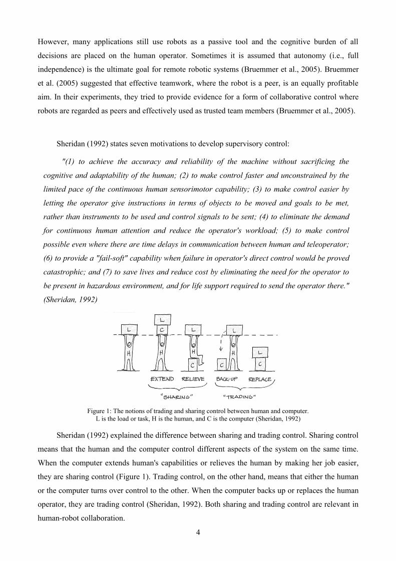
Figure 1: The notions of trading and sharing control between human and computer.
L is the load or task, H is the human, and C is the computer (Sheridan, 1992)
Sheridan (1992) explained the difference between sharing and trading control. Sharing control
means that the human and the computer control different aspects of the system on the same time.
When the computer extends human's capabilities or relieves the human by making her job easier,
they are sharing control (Figure 1). Trading control, on the other hand, means that either the human
or the computer turns over control to the other. When the computer backs up or replaces the human
operator, they are trading control (Sheridan, 1992). Both sharing and trading control are relevant in
human-robot collaboration.
5
A main issue in space exploration is to decide what human or robotic system (or a suitable
combination of the two) is most appropriate to use in those exploration tasks (Rodriguez and
Weisbin, 2003). Rodriguez and Weisbin (2003) introduced a method to evaluate systematically the
relative performance of some optional human-robot systems, in order to decide which type of assets
to use in a given situation. First, they decompose the space scenario that needs to be analyzed into a
set of major functional operations. For each of the functional operations, they define a set of
performance metrics to be used in the evaluation. Then they specify the agents (robot, human or a
combination) to be evaluated, together with the resources needed for their implementation. The
performance of each agent is then evaluated for each of the functional operations, and a score,
which estimates the aptitude of each agent for each operation, is determined. A composite score is
then computed for each agent and a comparison between systems' performances is done.
2.3 Collaboration types and levels
As aforementioned, automation refers to the full or partial replacement of a function
previously carried out by a human operator (Parasuraman et al., 2000). This means that automation
can differ from the lowest level of manual performance through some levels of collaboration
between the human and the robot up to the highest level of full autonomy (Parasuraman et al.,
2000).
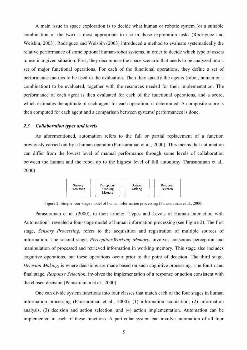
Figure 2: Simple four-stage model of human information processing (Parasuraman et al., 2000)
Parasuraman et al. (2000), in their article: "Types and Levels of Human Interaction with
Automation", revealed a four-stage model of human information processing (see Figure 2). The first
stage, Sensory Processing, refers to the acquisition and registration of multiple sources of
information. The second stage, Perception/Working Memory, involves conscious perception and
manipulation of processed and retrieved information in working memory. This stage also includes
cognitive operations, but these operations occur prior to the point of decision. The third stage,
Decision Making, is where decisions are made based on such cognitive processing. The fourth and
final stage, Response Selection, involves the implementation of a response or action consistent with
the chosen decision (Parasuraman et al., 2000).
One can divide system functions into four classes that match each of the four stages in human
information processing (Parasuraman et al., 2000): (1) information acquisition, (2) information
analysis, (3) decision and action selection, and (4) action implementation. Automation can be
implemented in each of these functions. A particular system can involve automation of all four
6
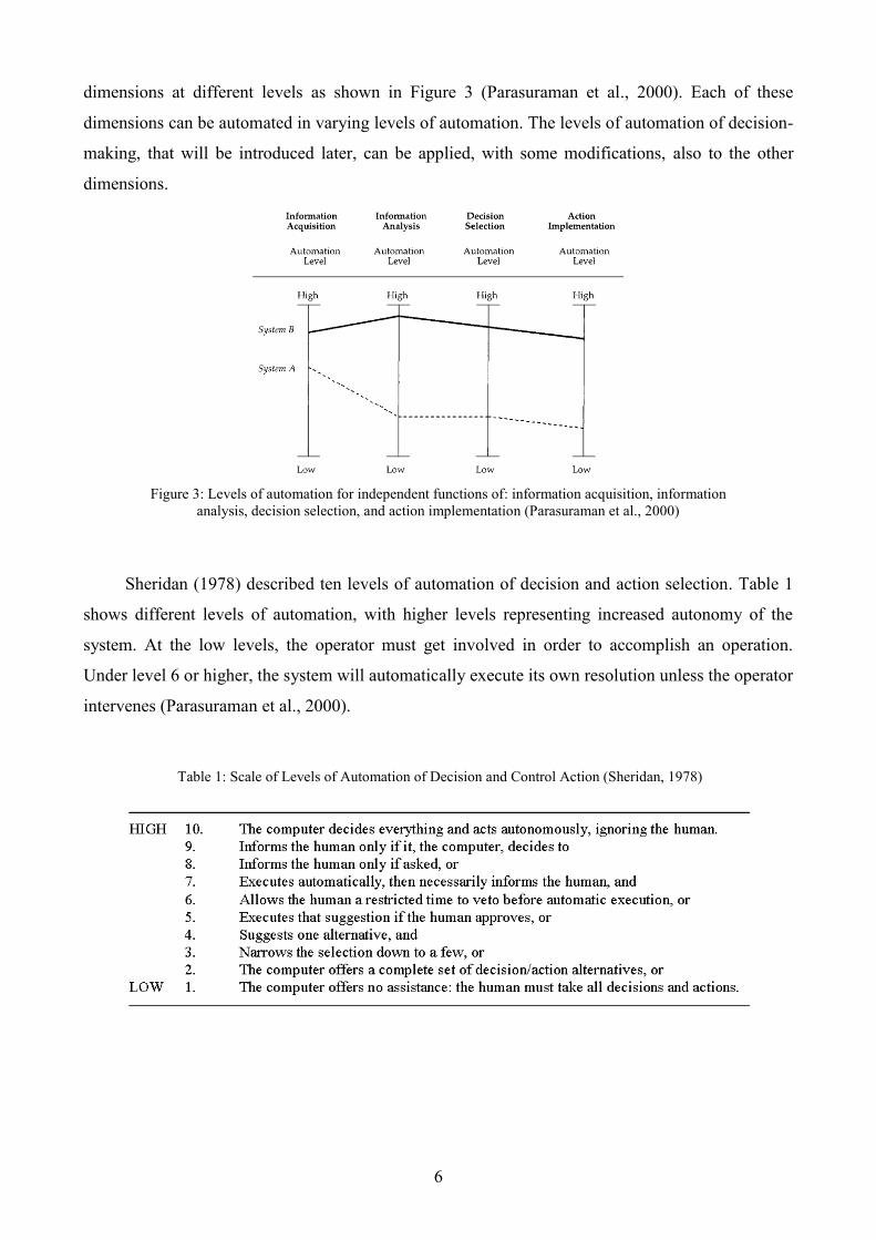
dimensions at different levels as shown in Figure 3 (Parasuraman et al., 2000). Each of these
dimensions can be automated in varying levels of automation. The levels of automation of decision-
making, that will be introduced later, can be applied, with some modifications, also to the other
dimensions.
Figure 3: Levels of automation for independent functions of: information acquisition, information
analysis, decision selection, and action implementation (Parasuraman et al., 2000)
Sheridan (1978) described ten levels of automation of decision and action selection. Table 1
shows different levels of automation, with higher levels representing increased autonomy of the
system. At the low levels, the operator must get involved in order to accomplish an operation.
Under level 6 or higher, the system will automatically execute its own resolution unless the operator
intervenes (Parasuraman et al., 2000).
Table 1: Scale of Levels of Automation of Decision and Control Action (Sheridan, 1978)
7
2.4 Examples of collaboration levels
Levels of collaboration are sometimes referred to as modes of operation of the given human-
robot system. Following we describe examples of collaboration levels implementations in different
applications. All of the examples include fully autonomy and fully manually levels, which consist
of a single collaborator without any cooperation. The collaboration levels differ by nature, scale,
structure, and number of levels.
Bechar and Edan (2000) evaluated two collaboration levels for agriculture robot guidance
through an off-road path. Two different guidance methods were tested: Directional guidance, where
the gross direction of advance is being marked and Waypoint guidance, where the system draws the
desired course of advancing along the path. Two collaboration levels were examined for each
guidance method: HO, where the human-operator marks the desired direction/course solely; and
HO-Rr, here the human-operator marks the desired direction/course with recommendations from the
robot (Bechar & Edan, 2000).
Bruemmer et al. (2005) defined four control modes of a remote mobile robot in an in-door
search and exploration task. (1) Tele Mode is a fully manually mode of operation, in which the
operator controls all robot movements. (2) Safe Mode is similar to Tele Mode. However, in Safe
Mode the robot is equipped with a level of initiative that prevents the operator from colliding with
obstacles. (3) Shared Mode, the robot can relieve the operator from the burden of direct control,
using reactive navigation to find a path based on perception of the environment. The robot accepts
operator intervention and supports dialogue using a finite number of scripted suggestions (e.g.,
“Path blocked! Continue left or right?”), that appear in a text box within the graphical interface. (4)
Autonomous Mode consists of series of high-level tasks such as patrol, search region or follow path.
In this mode, the only user intervention occurs on the tasking level; the robot itself manages all
decision-making and navigation (Bruemmer et al., 2005).
Bechar (2006) developed four collaboration levels for target recognition: Fully autonomous
level (R), in which the robot fulfills the task all by itself; and fully manually level (H), where the
human-operator does not use any help of the robot. Two more levels define collaboration between
the human operator and the robot. The first one (HR) is a collaboration level where the robot
indicates potential targets and the human operator at the following stage needs to mark the targets
he thinks are real and to add marks of targets the robot did not indicate. In the second collaboration
level (HOR), the human supervises the robot. The robot itself marks targets and the human operator
checks its' marks. The human operator unmarks targets that are not real and mark targets that the
robot missed (Bechar, 2006).
8
Hughes and Lewis (2005) designed a remote robotic system for a search and exploration task.
In order to control the robot, one or two cameras feed the human operator with live video from the
remote environment. Hughes and Lewis used two different levels of control on the cameras. At the
first one, Sensor-Driven Orientation, the operator supervises the camera while a guided-orientation
system recommends it where to look. Whenever the operator wants to, she can take control over the
camera, overriding system's recommendations. The other level, User-Controlled Orientation, the
camera is all the time under operator's control.
Czarnecki and Graves (2000) described a scale of five human-robot interaction levels for a
telerobotic behavior based system.
Most of these applications determine the best collaboration level for specific system and
mission conditions. Experiments were conducted in order to compare performance under different
levels of collaboration. Generally, the main conclusion was that systems perform better, in different
aspects, when human and robot collaborate. Moreover, the level of autonomy should not be
arbitrary and the user should be able to set robot's level of autonomy according to environment or
task constraints (Steinfeld, 2004). Team members (humans and robots) must recognize changing
situations and adapt the best collaboration level to ensure that the mission is done successfully
(Bruke et al., 2004). An expansion of Bechar's research (2006) will follow in the next section.
2.5 Collaboration in target recognition tasks
Target recognition is a common and critical element in most robotic systems (Bechar, 2006).
For example, the detection of parts in assembly lines, the detection of landmarks in autonomous
navigation, or the detection of fruits for robotic harvesters. Target recognition is a common and
important topic in many other research areas such as medical and brain research, quality assurance,
human factors, agriculture and remote sensing (Bechar, 2006). Automatic target recognition in
agriculture environment is characterized by low detection rates and high false alarm rates due to the
unstructured nature of both the environment and the objects (Bechar & Edan, 2003).
Target recognition is a mission in which the system needs to mark objects as targets (Bechar,
2006). Typical systems for target recognition use a sequence of algorithms that operate in different
stages in order to achieve recognition (Bhanu et al., 2000). A vision analysis based algorithm is
used in order to decide whether an object is a target or not (Bulanon et al, 2001). For example,
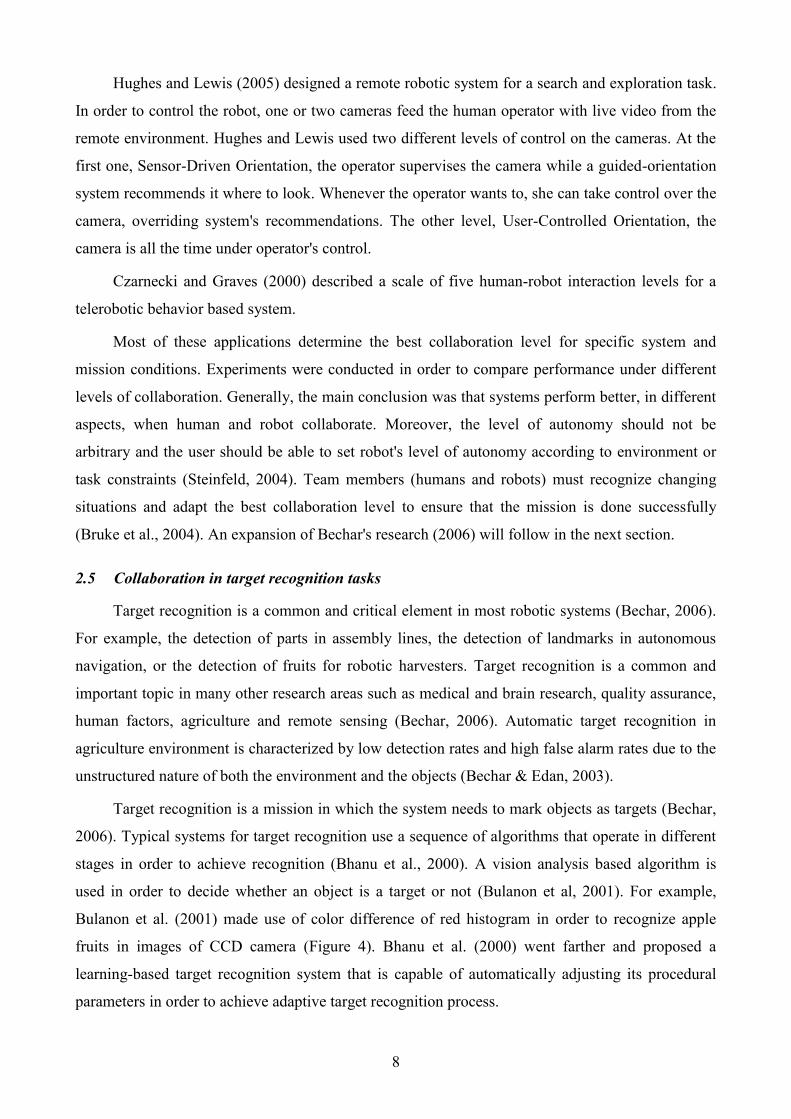
Bulanon et al. (2001) made use of color difference of red histogram in order to recognize apple
fruits in images of CCD camera (Figure 4). Bhanu et al. (2000) went farther and proposed a
learning-based target recognition system that is capable of automatically adjusting its procedural
parameters in order to achieve adaptive target recognition process.

9
Figure 4: Vision analysis for apple fruit detection (Bulanon et al, 2001)
(a) CCD image, (b) segmentation of color difference of red, (c) color difference of red histogram
Bechar, in his Ph.D. thesis (2006), examined human-robot collaboration for target
recognition. Four collaboration levels were defined and a method to determine the best
collaboration level was evaluated. To measure system performance under different collaboration
levels an objective function has been developed (Bechar, 2006). The objective function includes
five parts: hit (correct detection), false alarm, miss, correct rejection, and operational cost. Each of
the first four parts represents penalties or rewards of the recognition process. For instance, when a
correct detection occurs, meaning a real target was detected by the system, a reward is summed to
the objective function. Likewise, a penalty is taken into account when a target is missed or when the
system makes false alarm, marking a non-target as a target (Bechar, 2006).
Bechar (2006) found that the H collaboration level is never the best collaboration level
probably due to its high operational cost and low hit rate relative to the other collaboration levels.
Thus, collaboration of human and robot in target recognition tasks will always improve the optimal
performance. The combination of both human and robot in the HOR collaboration level increases
the system sensitivity in most cases and increases the probability of a hit while reducing the
probability of false alarms. In addition, findings indicated that when robot sensitivities are higher
than human sensitivities the best collaboration level is R (Bechar, 2006).
Oren, in his B.Sc final project (2007), continued Bechar's work and performed sensitivity
analyses of the objective function in order to understand how changes in different parameters
(human, robot, task, and environment) influence performance of the integrated human-robot system.
Oren et al. (2008) found that an increase in human and/or robot sensitivity causes an increase
in the objective function score and in fact, increases system's performance. Superior sensitivity
means better capability to discriminate between a signal (target) and a noise (no target) and
therefore, more hits and fewer false alarms occur (Oren et al., 2008). In addition, a sensitivity
analysis of the thresholds (see interpretation in Signal Detection Theory subchapter, 2.7) exposed
that in some cases, a small deviation from the optimal value causes shifts in the best collaboration
level.
10
2.6 Collaborative model for target recognition (Bechar, 2006)
This chapter details the objective function of the collaborative model developed by Bechar
(2006) for target recognition tasks.
The objective function describes the expected value of system performance, given the
properties of the environment and the system. The goal is to maximize the objective function. The
value of the objective function can be translated into a monetary value. The objective function
composed of the four responses of the target detection process and the system operational costs:
Is Hs Ms FAs CRs TsV V V V V V
Where HsV is the gain for target detections (hit), FAsV is the penalty for false alarms (FA), MsV
is the system penalty for missing targets (miss), CRsV is the gain for correct rejections (CR), and TsV
is the system operation cost. All gain, penalty and cost values have the same units, which enable us
to add them together to a single value, expressed in the objective function.
The gain and penalty functions are:
Hs S Hs HV N P P V
Ms S Ms MV N P P V
FAs S FAs FAV N (1 P ) P V
CRs S CRs CRV N (1 P ) P V
Where, N is the number of objects in the observed image and SP is the probability of an
object becoming a target. The third parameter in the equations, XsP , is the system probability for one
of the outcomes: hit, miss, false alarm or correct rejection ( X can be H , M , FA, CR ). The fourth
parameter, XV , is the system gain or penalty from the expected outcome.

11
The system‟s probability of a certain outcome is influenced from the serial structure of the
model and is composed of the robot and the human probabilities:
Hs Hr Hrh Hr Hh(1 )P P P P P
Ms Mr Mh Mr Mrh(1 )P P P P P
FAs FAr FArh FAr FAh(1 )P P P P P
CRs CRr CRh CRr CRrh(1 )P P P P P
Where,
(1) HrP is the robot probability of a hit,
(2) HrhP is the human probability of confirming a robot hit,
(3) HhP is the human probability of detecting a target that the robot did not detect,
(4) MrP is the robot miss probability,
(5) MrhP is the human probability of un-confirming a robot hit,
(6) MhP is the human probability of missing a target the robot missed,
(7) FArP is the robot false alarm probability,
(8) FArhP is the human probability of not correcting a robot false alarm,
(9) FAhP is the human probability of a false alarm on targets the robot correctly rejected,
(10) CRrP is the robot probability of a correct rejection,
(11) CRrhP is the human probability of correcting a robot false alarm, and
(12) CRhP is the human probability of a correct rejection on targets the robot correctly rejected.
The sum of hit and miss probabilities (of the same type) equals one, so does the sum of false
alarm and correct rejection probabilities.
The system‟s operation cost is:
Ts S t S Hs S FAs CV t V [ N P P N (1 P ) P ] V
Where, St is the time required by the system to perform a task, tV is the cost of one time unit,
and CV is the operation cost of one object recognition (hit or false alarm).
12
The system time consists of the time it takes the human to decide whether to confirm or reject
robot detections; and the time it takes the human to decide whether objects not detected by the robot
are targets or not. The robot operation time, rt , of processing the images and performing hits or
false alarms, is also included.
S S Hr Hrh Hrh S Hr Hh Hh
S Hr Hrh Mrh S Hr Hh Mh
S FAr FArh FArh S FAr FAh FAh
S FAr FArh CRrh S FAr
t N P P P t N P (1 P ) P t
N P P (1 P ) t N P (1 P ) (1 P ) t
N (1 P ) P P t N (1 P ) (1 P ) P t
N (1 P ) P (1 P ) t N (1 P ) (1 P ) (1 P
FAh CRh r) t N t
Where,
(1) Hrht is the human time required to confirm a robot hit,
(2) Hht is the human time required to hit a target that the robot did not hit,
(3) Mrht is the human time lost when a robot hit is missed,
(4) Mht is the human time invested when missing a target that the robot did not hit,
(5) FArht is the human time needed not to correct a robot false alarm,
(6) FAht is the human false alarm time,
(7) CRrht is the human time to correctly reject a robot false alarm,
(8) CRht is the human correct rejection time, and (9) rt is the robot operation time.
Explicit expression of the system objective function, IsV , suitable for all collaboration levels, is:
Is S Hr Hrh H C Hrh t Hr Hh H C Hh t
S Hr Hrh M Mrh t Hr Hh M Mh t
S FAr FArh FA C FArh t FAr FAh FA C FAh t
V N P [ P P (V V t V ) (1 P ) P (V V t V )]
N P [ P (1 P ) (V t V ) (1 P ) (1 P ) (V t V )]
N (1 P ) [ P P (V V t V ) (1 P ) P (V V t V )]
N
S FAr FArh CR CRrh t FAr FAh CR CRh t r t(1 P ) [ P (1 P ) (V t V ) (1 P ) (1 P ) (V t V )] N t V
For the H collaboration level, the system objective function will be a degenerate form of the full
objective function, and will not include the robot variables:
Is S Hh H C Hh t Hh M Mh t
S FAh FA C FAh t FAh CR CRh t
V N P [ P (V V t V ) (1 P ) (V t V )]
N (1 P ) [ P (V V t V ) (1 P ) (V t V )]
In the R collaboration level, the system objective function will be a degenerate form of the full
objective function, and will not include the human variables:
Is S Hr H C Hr M
S FAr FA C FAr CR r t
V N P [ P (V V ) (1 P ) V ]
N (1 P ) [ P (V V ) (1 P ) V ] N t V
13
2.7 Signal detection theory
This section gives a tutorial for the signal detection theory.
"Reading in a coffee shop, you see someone who looks familiar. Have you met him
before? Should you go and talk to him at the risk of embarrassment when you realize he is a
stranger? On the other hand, should you pretend to ignore him at the risk of offending your
friend? Both paths of action have potential costs and benefits and the correct decision is not
clear. Furthermore, the decision you make might be biased by your own previous experience.
For example, if in the past you accidentally waved 'hello' to a strange, then you might be less
likely to wave to the person who looks familiar" (http://wise.cgu.edu).
This is an example of detection process. A common dimension of these situations is that there
is doubt whether a signal is present or not (Sheridan, 1992). Signal detection theory provides a
general framework to describe and study decisions that are made in ambiguous situations (Wickens,
2002). This decision theory tries to estimate decision-making processes for binary categorization
decisions, i.e., Yes/No or True/False. It is specifically concerned with how these choices are, or
should be made under uncertain conditions (Brown & Davis, 2006).
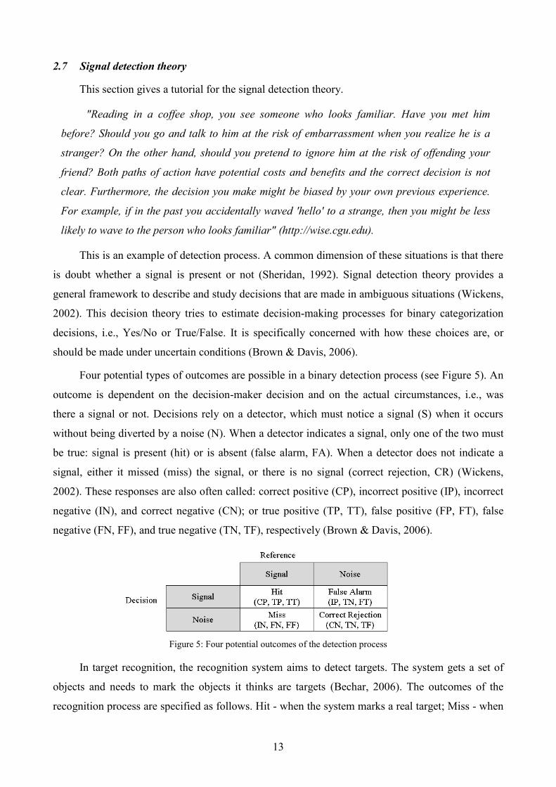
Four potential types of outcomes are possible in a binary detection process (see Figure 5). An
outcome is dependent on the decision-maker decision and on the actual circumstances, i.e., was
there a signal or not. Decisions rely on a detector, which must notice a signal (S) when it occurs
without being diverted by a noise (N). When a detector indicates a signal, only one of the two must
be true: signal is present (hit) or is absent (false alarm, FA). When a detector does not indicate a
signal, either it missed (miss) the signal, or there is no signal (correct rejection, CR) (Wickens,
2002). These responses are also often called: correct positive (CP), incorrect positive (IP), incorrect
negative (IN), and correct negative (CN); or true positive (TP, TT), false positive (FP, FT), false
negative (FN, FF), and true negative (TN, TF), respectively (Brown & Davis, 2006).
Figure 5: Four potential outcomes of the detection process
In target recognition, the recognition system aims to detect targets. The system gets a set of
objects and needs to mark the objects it thinks are targets (Bechar, 2006). The outcomes of the
recognition process are specified as follows. Hit - when the system marks a real target; Miss - when
14
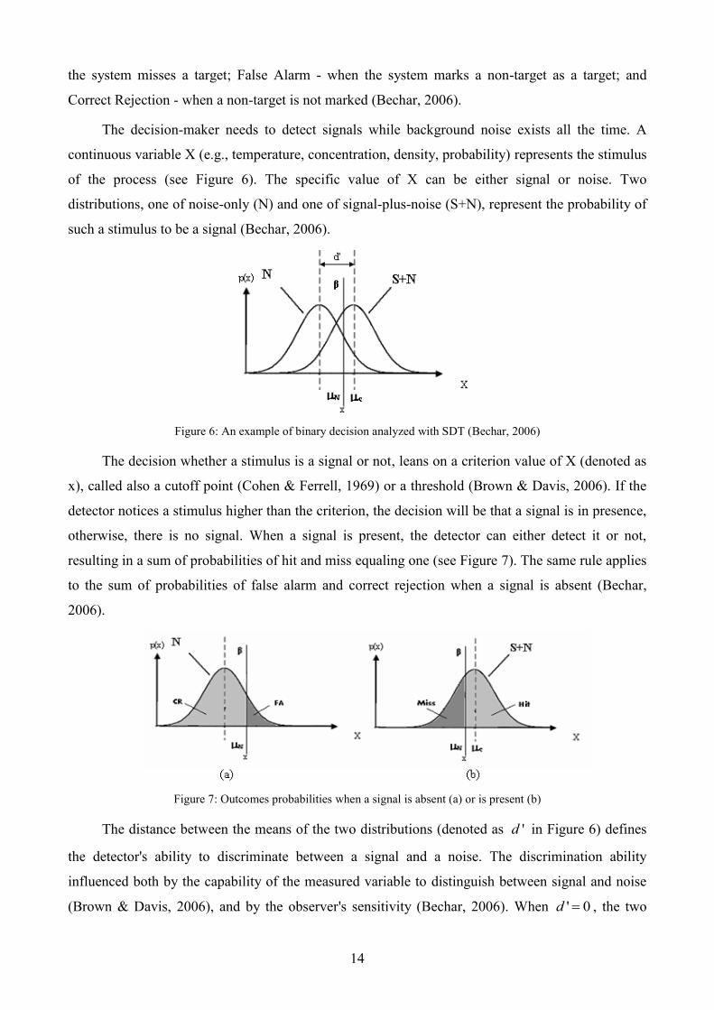
the system misses a target; False Alarm - when the system marks a non-target as a target; and
Correct Rejection - when a non-target is not marked (Bechar, 2006).
The decision-maker needs to detect signals while background noise exists all the time. A
continuous variable X (e.g., temperature, concentration, density, probability) represents the stimulus
of the process (see Figure 6). The specific value of X can be either signal or noise. Two
distributions, one of noise-only (N) and one of signal-plus-noise (S+N), represent the probability of
such a stimulus to be a signal (Bechar, 2006).
Figure 6: An example of binary decision analyzed with SDT (Bechar, 2006)
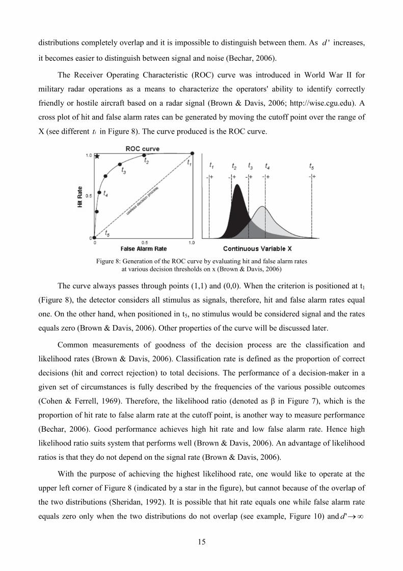
The decision whether a stimulus is a signal or not, leans on a criterion value of X (denoted as
x), called also a cutoff point (Cohen & Ferrell, 1969) or a threshold (Brown & Davis, 2006). If the
detector notices a stimulus higher than the criterion, the decision will be that a signal is in presence,
otherwise, there is no signal. When a signal is present, the detector can either detect it or not,
resulting in a sum of probabilities of hit and miss equaling one (see Figure 7). The same rule applies
to the sum of probabilities of false alarm and correct rejection when a signal is absent (Bechar,
2006).
Figure 7: Outcomes probabilities when a signal is absent (a) or is present (b)
The distance between the means of the two distributions (denoted as 'd in Figure 6) defines
the detector's ability to discriminate between a signal and a noise. The discrimination ability
influenced both by the capability of the measured variable to distinguish between signal and noise
(Brown & Davis, 2006), and by the observer's sensitivity (Bechar, 2006). When ' 0d , the two
15
distributions completely overlap and it is impossible to distinguish between them. As 'd increases,
it becomes easier to distinguish between signal and noise (Bechar, 2006).
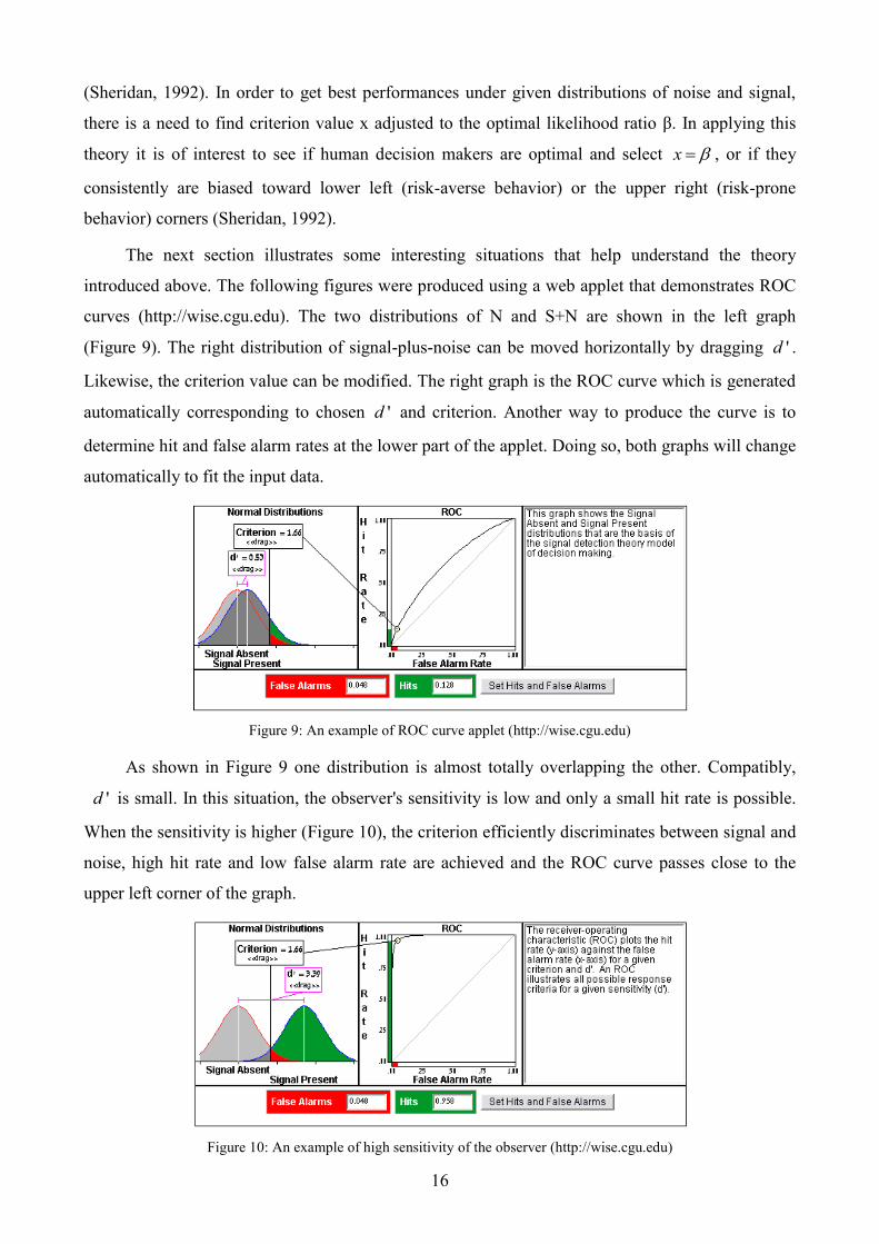
The Receiver Operating Characteristic (ROC) curve was introduced in World War II for
military radar operations as a means to characterize the operators' ability to identify correctly
friendly or hostile aircraft based on a radar signal (Brown & Davis, 2006; http://wise.cgu.edu). A
cross plot of hit and false alarm rates can be generated by moving the cutoff point over the range of
X (see different it in Figure 8). The curve produced is the ROC curve.
Figure 8: Generation of the ROC curve by evaluating hit and false alarm rates
at various decision thresholds on x (Brown & Davis, 2006)
The curve always passes through points (1,1) and (0,0). When the criterion is positioned at t1
(Figure 8), the detector considers all stimulus as signals, therefore, hit and false alarm rates equal
one. On the other hand, when positioned in t5, no stimulus would be considered signal and the rates
equals zero (Brown & Davis, 2006). Other properties of the curve will be discussed later.
Common measurements of goodness of the decision process are the classification and
likelihood rates (Brown & Davis, 2006). Classification rate is defined as the proportion of correct
decisions (hit and correct rejection) to total decisions. The performance of a decision-maker in a
given set of circumstances is fully described by the frequencies of the various possible outcomes
(Cohen & Ferrell, 1969). Therefore, the likelihood ratio (denoted as β in Figure 7), which is the
proportion of hit rate to false alarm rate at the cutoff point, is another way to measure performance
(Bechar, 2006). Good performance achieves high hit rate and low false alarm rate. Hence high
likelihood ratio suits system that performs well (Brown & Davis, 2006). An advantage of likelihood
ratios is that they do not depend on the signal rate (Brown & Davis, 2006).
With the purpose of achieving the highest likelihood rate, one would like to operate at the
upper left corner of Figure 8 (indicated by a star in the figure), but cannot because of the overlap of
the two distributions (Sheridan, 1992). It is possible that hit rate equals one while false alarm rate
equals zero only when the two distributions do not overlap (see example, Figure 10) and 'd
16
(Sheridan, 1992). In order to get best performances under given distributions of noise and signal,
there is a need to find criterion value x adjusted to the optimal likelihood ratio β. In applying this
theory it is of interest to see if human decision makers are optimal and select x , or if they
consistently are biased toward lower left (risk-averse behavior) or the upper right (risk-prone
behavior) corners (Sheridan, 1992).
The next section illustrates some interesting situations that help understand the theory
introduced above. The following figures were produced using a web applet that demonstrates ROC
curves (http://wise.cgu.edu). The two distributions of N and S+N are shown in the left graph
(Figure 9). The right distribution of signal-plus-noise can be moved horizontally by dragging 'd .
Likewise, the criterion value can be modified. The right graph is the ROC curve which is generated
automatically corresponding to chosen 'd and criterion. Another way to produce the curve is to
determine hit and false alarm rates at the lower part of the applet. Doing so, both graphs will change
automatically to fit the input data.
Figure 9: An example of ROC curve applet (http://wise.cgu.edu)
As shown in Figure 9 one distribution is almost totally overlapping the other. Compatibly,
'd is small. In this situation, the observer's sensitivity is low and only a small hit rate is possible.
When the sensitivity is higher (Figure 10), the criterion efficiently discriminates between signal and
noise, high hit rate and low false alarm rate are achieved and the ROC curve passes close to the
upper left corner of the graph.
Figure 10: An example of high sensitivity of the observer (http://wise.cgu.edu)
17
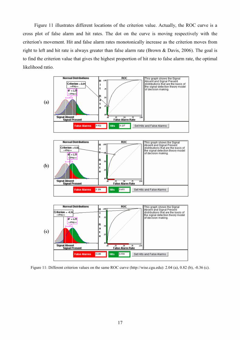
Figure 11 illustrates different locations of the criterion value. Actually, the ROC curve is a
cross plot of false alarm and hit rates. The dot on the curve is moving respectively with the
criterion's movement. Hit and false alarm rates monotonically increase as the criterion moves from
right to left and hit rate is always greater than false alarm rate (Brown & Davis, 2006). The goal is
to find the criterion value that gives the highest proportion of hit rate to false alarm rate, the optimal
likelihood ratio.
Figure 11: Different criterion values on the same ROC curve (http://wise.cgu.edu): 2.04 (a), 0.82 (b), -0.36 (c).

18
19
2.8 Reaction time models
Signal detection theory, which was introduced above, provides a general framework to
describe decisions and how they should be made under uncertain conditions (Brown & Davis,
2006). Signal detection theory models provide an account of accuracy only, and are not concerned
with the time it takes the observer to make the decision1 (Ratcliff & Smith, 2004).
“Reaction time, that is the time from the onset of a stimulus or signal to the initiation of
response, has been recognized as a potentially powerful means of relating mental events to
physical measures. ... More recent developments have enhanced the value of reaction time as a
measure rather than diminished it (Welford, 1980)”.
The relation between response time and accuracy is not constant; it varies according to
whether speed or accuracy of performance is emphasized and according to whether one response or
another is more probable or weighted more heavily (Ratcliff & Rouder, 1998). Therefore, previous
models have dealt with only one measure, accuracy or response time (Ratcliff & Rouder, 1998).
Various models were proposed to account for reaction time and accuracy. Ratcliff and
Rounder (1998) introduced the diffusion model which is a sequential-sampling model and can
explain the relationship between correct and error responses while at the same time fitting all the
other response time and response probability aspects of the data. Sequential sampling models are
unique in providing a way to understand both the speed and accuracy of performance within a
common theoretical framework (Ratcliff & Smith, 2004).
Ratcliff, Mckoon and Zandt (1999) also claim that the main difficulty in recent modeling is
that two dependent variables, reaction time and the probability of responses, must to be modeled in
the same integrated framework. They introduced connectionist models that explain how cognitive
tasks are learned. Learning is the result of many individual trials with stimuli, each trial with
feedback about whether the model's response was correct or not (Ratcliff et al., 1999).
Pike (1973) suggested that latency in response is some inverse function of distance from the
criteria, and that latency decreases with the distance. According to Pike (1973), successful
description of response latency is necessary for verification of the detection model.
1 Response Time, Response Latency and Decision Time, refer to the common term Reaction Time, which is used to
describe the time it takes the observers to decide about an observed object.
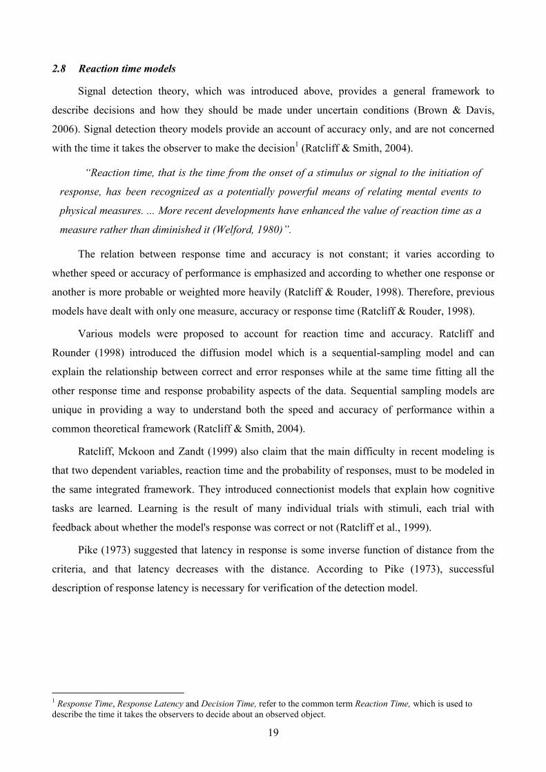
20
Murdock (1985) analyzed the strength-latency relationship and introduced a generic reaction
time model based on the distance-from-criteria of the observed object. He suggested that an
exponential function is the most reasonable to use in order to transfer the object‟s strength, i.e.,
distance-from-criteria, into latency (Figure 12). Exponential functions can describe symmetrical
descendent of latency on both sides of the yes/no criterion (Murdock, 1985).
Figure 12: Signal (x) is normally distributed with criterion Xco. Exponential
transfer function maps signal strength into latency (t), and the resulting latency
distribution f(t) is shown by the dots (Murdock, 1985).
21
3 METHODOLOGY
3.1 Overview
This thesis continues a previous work of Bechar (2006) which focused on developing a
human-robot collaboration model for target recognition task. The objective function of the model
describes the system score for a given collaboration level and determines the best collaboration
level for a given set of parameters. This thesis expands the objective function of the model by
incorporating a function for human reaction time instead of a constant value. In this thesis, we
check the influence of the reaction time on the objective function score and the best collaboration
level.
A reaction time model is developed and integrated into the collaboration model. Numerical
and sensitivity analysis of the new model is conducted using simulated data.
3.2 Reaction time model development
The objective function of the model developed by Bechar (2006), takes into account the costs
related to the time it takes a human-robot system to perform a target detection task. Implementing a
detection procedure by the human consist of two stages. First, the human must decide whether an
object is target or not. The action on the second stage depends on the human decision and on the
collaboration level as follows. In some cases, the human needs to make a motoric action in order to
mark or unmark an object (e.g., confirming a robot recommendation in the HR collaboration level,
or canceling a wrong robot's mark in the HOR collaboration level). In other cases, the human does
not have to perform a motoric action (i.e., when the robot's recommendation is not a real target in
the HR collaboration level, or when the robot decided correct in the HOR collaboration level). The
time the first stage takes is the reaction time of the human.
Previous work (Bechar, 2006) considered a constant value for the reaction time. This research
introduces further development of the model taking into consideration the fact that the reaction time
of the human depends on the strength of the observed object (i.e., the distance of the observed
object from the cutoff point). In this research, we incorporate a reaction time model, based on
Murdock (1985), into Bechar‟s model.
Furthermore, a mathematical development of a mean distance model is introduced. The model
is based on the signal detection theory model, and calculates the mean distance between the cutoff
point and objects of the same category (e.g., mean distance of all objects that were 'missed').

22
3.3 Performance measures
This research uses the nine performance measures defined by Bechar (2006). Eight
performance measures represent the target identification possible outcomes. Four of them stand for
objects the robot marked as targets (i.e., hit, miss, false alarm and correct rejection) and the other
four stands for objects the robot did not mark. The ninth performance measure is the time required
for the human-robot integrated system to fulfill the task. The system objective function combines all
performance measures into a single parameter.
3.4 Numerical analysis
A numerical analysis is implemented on a personal computer with Matlab 7™, and detailed in
chapter 5. The objective is to determine the best collaboration levels for different human, robot, and
task characteristics, and to examine the influence of the time component.
The analysis is focused on three different system types. The first two types, introduced by
Oren (2007), give high emphasis of not causing one of the two possible errors in target recognition:
missing targets or making false alarms. The third type gives the same importance for all possible
outcomes.
3.5 Sensitivity analysis
The numerical analysis is conducted only for the cases in which the human and the robot
perform optimally, i.e., optimal cutoff points of the human and the robot. The target detection
process of the robot is computerized and it is possible to adjust its cutoff point during the task
according to changes in the environment. On the other hand, an optimal cutoff point of the human is
less obvious and it is much more difficult to be manipulated. Therefore, the work includes an in-
depth sensitivity analysis of the human and robot cutoff points. The analysis shows how small
changes in the cutoff point position, influence the objective function score and the best
collaboration level.

23
4 MODEL DEVELOPMENT
In this research, we incorporate a reaction time model, based on Murdock (1985), into
Bechar‟s collaboration model (2006). According to Murdock (1985), reaction time depends on the
strength of the observed object. The strength of an object is relative to the distance of the observed
object‟s value from the criteria. The distance of an object can be measured by the same units of the
measured object or by standard deviation units. Normalizing the signal and noise distributions helps
us to describe the problem in standard deviation units. It benefits in generalizing the problem rather
than using the actual units that fit only to a specific case. The cutoff point gets a different
interpretation for each normalized distribution. We denote the cutoff points as Sz and Nz for the
signal and the noise distributions, respectively.
;co S co NS N
S N
x xz z
A short review of the Normal and the Standard Normal distributions, as well as definitions of
signal and noise distributions is included in Appendix A.
For a matter of simplicity, all equations of the model will be defined first as functions of the
parameters Sz and Nz , and later on, for the numerical analysis, they will be expressed by the
likelihood ratio, β, between the signal and noise density functions in the cutoff point, cox , and the
distance between the means of the signal and noise distributions, d ' . See chapter 2.6 for details. All
expressions are included in Appendix B.
In this section, we introduce a development of a mean distance of all objects of the same
category (miss, hit, correct rejection, and false alarm). Then, we formulate the reaction time model
and incorporate it into the human-robot collaboration model.
4.1 Mean distance model
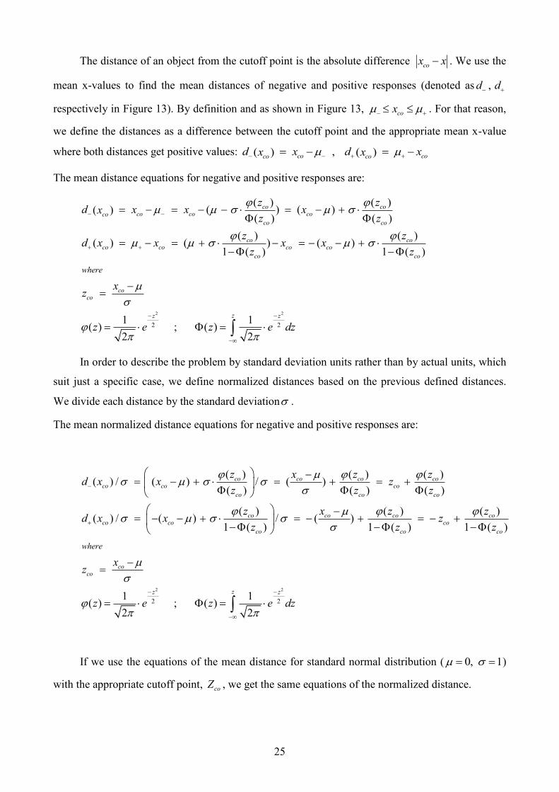
4.1.1 Mean x-values and distances in a normal distribution
In the recognition process, the system marks an object as a target if the object‟s value is
higher than the cutoff point value (denoted as cox in Figure 13). We use the term „Positive
Response‟ to describe objects that the system marks. Positive response can be either a hit, if the
object is a target; or a false alarm if it is not. The term „Negative Response‟ describes objects with a
value lower than the cutoff point value, which the system does not mark as targets. A negative
response can be either a miss, if the object is a target; or a correct rejection if it is not. The mean x-
value of all negative responses is denoted as , and the mean x-value of all positive responses is
denoted as .
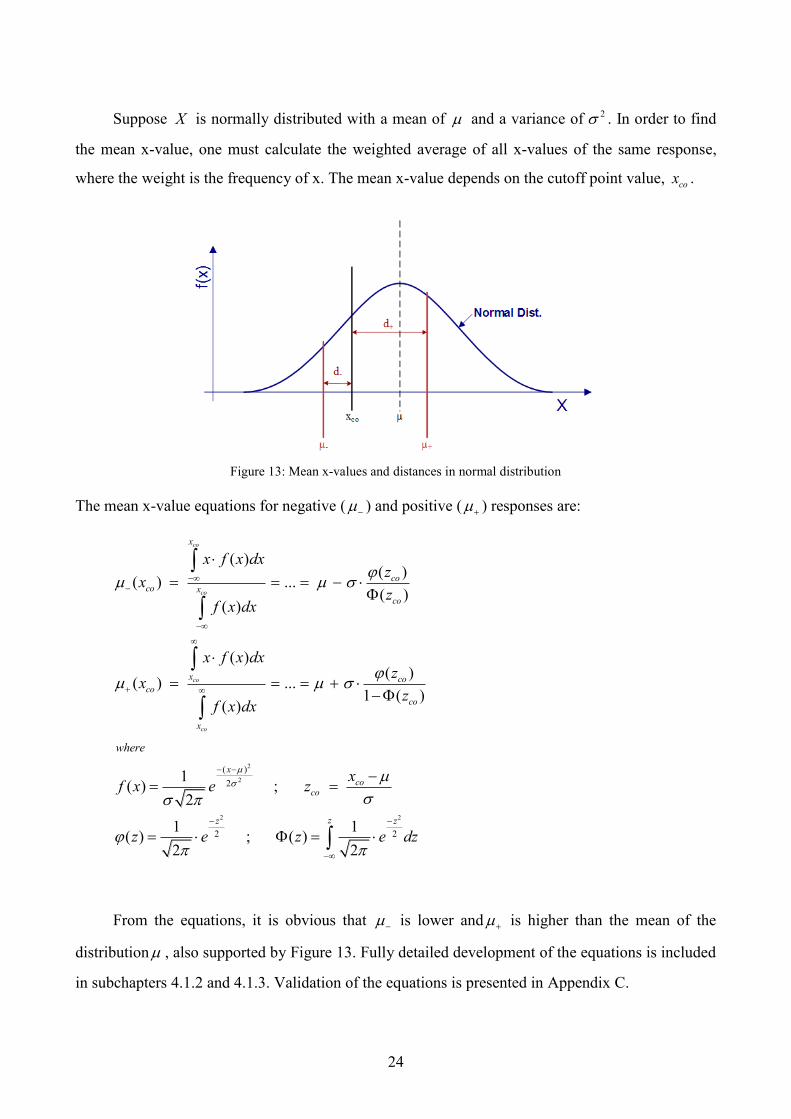
24
Suppose X is normally distributed with a mean of and a variance of 2 . In order to find
the mean x-value, one must calculate the weighted average of all x-values of the same response,
where the weight is the frequency of x. The mean x-value depends on the cutoff point value, cox .
Figure 13: Mean x-values and distances in normal distribution
The mean x-value equations for negative ( ) and positive ( ) responses are:
2
2
2 2
( )
2
2 2
( )( )
( ) ...( )
( )
( )( )
( ) ...1 ( )
( )
1( ) ;
2
1 1( ) ; ( )
2 2
co
co
co
co
x
coco x
co
x coco
co
x
x
coco
zz z
where
x f x dxz
xz
f x dx
x f x dxz
xz
f x dx
xf x e z
z e z e dz
From the equations, it is obvious that is lower and is higher than the mean of the
distribution , also supported by Figure 13. Fully detailed development of the equations is included
in subchapters 4.1.2 and 4.1.3. Validation of the equations is presented in Appendix C.
25
The distance of an object from the cutoff point is the absolute difference cox x . We use the
mean x-values to find the mean distances of negative and positive responses (denoted as ,d d
respectively in Figure 13). By definition and as shown in Figure 13, cox . For that reason,
we define the distances as a difference between the cutoff point and the appropriate mean x-value
where both distances get positive values: ,( ) ( )co coco cod x d xx x
The mean distance equations for negative and positive responses are:
2 2
2 2
( ) ( )( ) ( )( )
( ) ( )
( ) ( )( ) ( ) ( )
1 ( ) 1 ( )
1 1( ) ; ( )
2 2
co coco co coco
co co
co coco co co co
co co
coco
zz z
where
z zd x x xx
z z
z zd x x x x
z z
xz
z e z e dz
In order to describe the problem by standard deviation units rather than by actual units, which
suit just a specific case, we define normalized distances based on the previous defined distances.
We divide each distance by the standard deviation .
The mean normalized distance equations for negative and positive responses are:
2
2
( ) ( ) ( )( ) / ( ) / ( )
( ) ( ) ( )
( ) ( ) ( )( ) / ( ) / ( )
1 ( ) 1 ( ) 1 ( )
1( ) ; (
2
co co co coco co co
co co co
co co co coco co co
co co co
coco
z
where
z x z zd x x z
z z z
z x z zd x x z
z z z
xz
z e z
2
21
)2
z z
e dz
If we use the equations of the mean distance for standard normal distribution ( 0, 1 )
with the appropriate cutoff point, coZ , we get the same equations of the normalized distance.
26
To simplify the equations, we use the following symmetric rules of the standard normal
distribution:
2 2
2 2
( ) ( )
( ) 1 ( )
( ) 1 ( )
1 1( ) ; ( )
2 2
zz z
z z
z z
z z
where
z e z e dz
We define the function ( )z :
( )( )
( )
zz
z
Due to the symmetric rules, the function holds:
( ) ( )( )
( ) 1 ( )
z zz
z z
We use ( )z to define again the normalized distances as:
( )( ) / ( )
( )
( )( ) / ( )
1 ( )
coco co co co
co
coco S co co
co
zd x z z z
z
zd x z z z
z

27
4.1.2 Mathematical development of Mean x-value of negative responses
In order to find the mean x-value, one must calculate the weighted average of all x-values of
the same response, where the weight is the frequency of x.
2
2
2
2
2
( )
2
( )
2
1( )
2( )
1( )
2
:
( )
1( )
2
co co
co co
x x x
co x x x
coco co
z
x f x dx x e dx
x
f x dx e dx
Changing the domain of integration
xz x z
dx d zdx dz
dz dz
x z
xx x z z
z e
2
2 2
2 2 2 2
2 2 2
2 2
2 2
2 2 2 2
2 2 2
1( )
2
1 1
2 2
1 1 1 1
2 2 2 2
1 1 1
2 2 2
co co
co co
co co co co
co co co
z z z
z zz z
z z z zz z z z
z z zz z z
dz z e dz
e dz e dz
e dz z e dz e dz z e dz
e dz e dz e dz
From
2
2
:
1( )
2
coz z
co
the standard normal distribution
e dz z
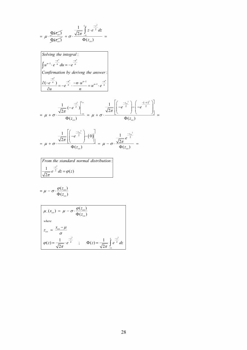
28
( )coz
( )coz
2
222
2
1
11
2 22
1
2
( )
:
:
( )
11( )
22
( )
co
n n
n
n n
coco
z z
co
u u
n n n
uu unn
nn u
z zz
co
z e dz
z
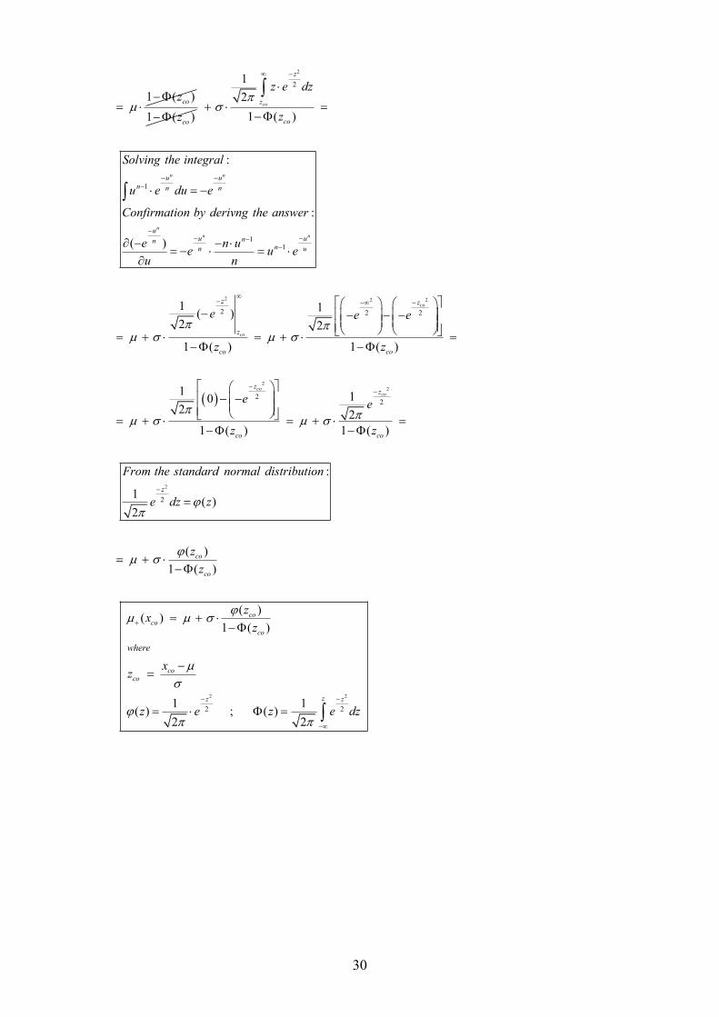
Solving the integral
u e du e
Confirmation by derivng the answer
e n ue u e
u n
e ee
z
2
2
2
2
22
2
2
( )
1 102 2
( ) ( )
:
1( )
2
( )
( )
( )( )
( )
1( ) ;
2
coco
co
zz
co co
z
co
co
coco
co
coco
z
where
z
e e
z z
From the standard normal distribution
e dz z
z
z
zx
z
xz
z e
2
21
( )2
z z
z e dz
29
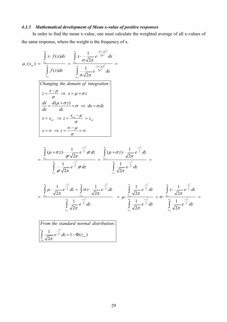
4.1.3 Mathematical development of Mean x-value of positive responses
In order to find the mean x-value, one must calculate the weighted average of all x-values of
the same response, where the weight is the frequency of x.
2
2
2
2
2
( )
2
( )
2
2
1( )
2( )
1( )2
:
( )
1( )
2
co co
co co
co
x
x x
co x
x x
coco co
z
z
x f x dx x e dx
x
f x dx e dx
Changing the domain of integration
xz x z
dx d zdx dz
dz dz
xx x z z
x z
z e dz
2
2 2
2 2 2 2
2 2 2
2
2 2
2 2 2 2
2 2 2
1( )
2
1 1
2 2
1 1 1 1
2 2 2 2
1 1 1
2 2 2
co
co co
co co co co
co co co
z
z
z z
z z
z z z z
z z z z
z z z
z z z
z e dz
e dz e dz
e dz z e dz e dz z e dz
e dz e dz e dz
From the standard normal
2
2
:
11 ( )
2
coz z
co
distribution
e dz z
30
1 ( )coz
1 ( )coz
2
2 22
2
1
11
2 2 2
1
2
1 ( )
:
:
( )
1 1( )
2 2
1 ( )
co
n n
n
n n
co
co
z
z
co
u u
n n n
uu unn
nn u
z z
z
co
z e dz
z
Solving the integral
u e du e
Confirmation by derivng the answer
e n ue u e
u n
e e e
z
2
2
2
22
2
1 ( )
1 102 2
1 ( ) 1 ( )
:
1( )
2
( )
1 ( )
( )( )
1 ( )
( )
coco
co
zz
co co
z
co
co
coco
co
coco
where
z
e e
z z
From the standard normal distribution
e dz z
z
z
zx
z
xz
z
2 2
2 21 1
; ( )2 2
zz z
e z e dz
31
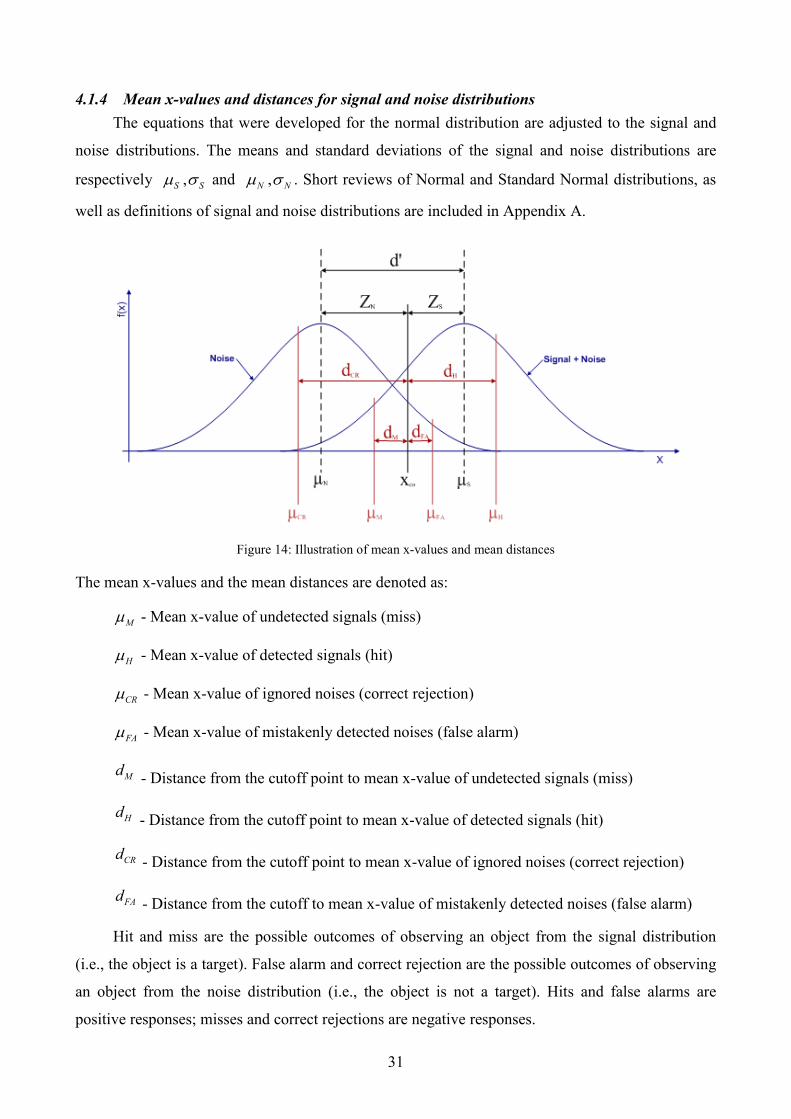
4.1.4 Mean x-values and distances for signal and noise distributions
The equations that were developed for the normal distribution are adjusted to the signal and
noise distributions. The means and standard deviations of the signal and noise distributions are
respectively ,S S and ,N N . Short reviews of Normal and Standard Normal distributions, as
well as definitions of signal and noise distributions are included in Appendix A.
Figure 14: Illustration of mean x-values and mean distances
The mean x-values and the mean distances are denoted as:
M - Mean x-value of undetected signals (miss)
H - Mean x-value of detected signals (hit)
CR - Mean x-value of ignored noises (correct rejection)
FA - Mean x-value of mistakenly detected noises (false alarm)
Md - Distance from the cutoff point to mean x-value of undetected signals (miss)
Hd - Distance from the cutoff point to mean x-value of detected signals (hit)
CRd - Distance from the cutoff point to mean x-value of ignored noises (correct rejection)
FAd - Distance from the cutoff to mean x-value of mistakenly detected noises (false alarm)
Hit and miss are the possible outcomes of observing an object from the signal distribution
(i.e., the object is a target). False alarm and correct rejection are the possible outcomes of observing
an object from the noise distribution (i.e., the object is not a target). Hits and false alarms are
positive responses; misses and correct rejections are negative responses.
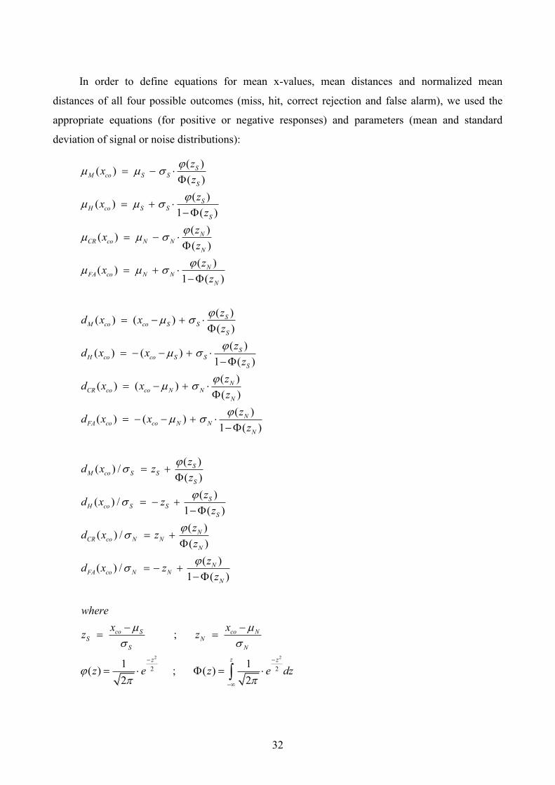
32
In order to define equations for mean x-values, mean distances and normalized mean
distances of all four possible outcomes (miss, hit, correct rejection and false alarm), we used the
appropriate equations (for positive or negative responses) and parameters (mean and standard
deviation of signal or noise distributions):
( )( )
( )
( )( )
1 ( )
( )( )
( )
( )( )
1 ( )
( )( ) ( )
( )
( )( ) ( )
1 ( )
( )( ) ( )
( )
(
SM co S S
S
SH co S S
S
NCR co N N
N
NFA co N N
N
SM co co S S
S
SH co co S S
S
NCR co co N N
N
FA
zx
z
zx
z
zx
z
zx
z
zd x x
z
zd x x
z
zd x x
z
d
2 2
2 2
( )) ( )
1 ( )
( )( ) /
( )
( )( ) /
1 ( )
( )( ) /
( )
( )( ) /
1 ( )
;
1 1( ) ; ( )
2 2
Nco co N N
N
SM co S S
S
SH co S S
S
NCR co N N
N
NFA co N N
N
co S co NS N
S N
zz z
zx x
z
zd x z
z
zd x z
z
zd x z
z
zd x z
z
where
x xz z
z e z e dz
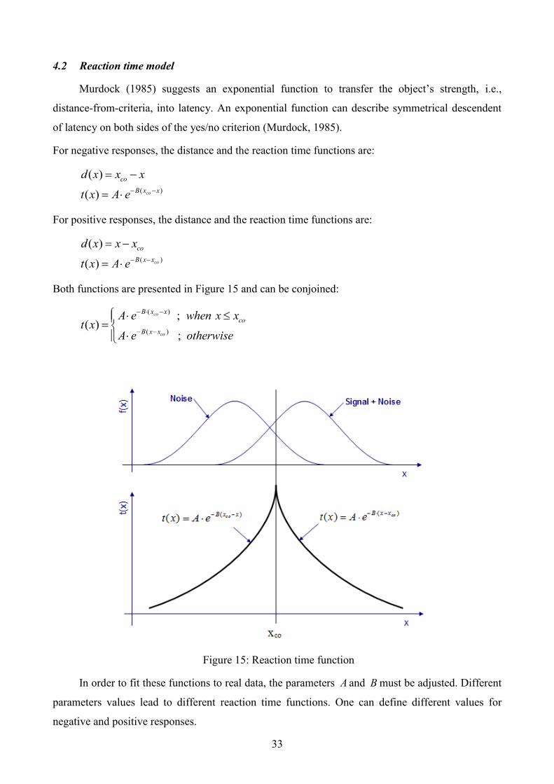
33
4.2 Reaction time model
Murdock (1985) suggests an exponential function to transfer the object‟s strength, i.e.,
distance-from-criteria, into latency. An exponential function can describe symmetrical descendent
of latency on both sides of the yes/no criterion (Murdock, 1985).
For negative responses, the distance and the reaction time functions are:
( )
( )
( ) co
co
B x x
d x x x
t x A e
For positive responses, the distance and the reaction time functions are:
( )
( )
( ) co
co
B x x
d x x x
t x A e
Both functions are presented in Figure 15 and can be conjoined:
( )
( )
;( )
;
co
co
B x x
co
B x x
A e when x xt x
A e otherwise
Figure 15: Reaction time function
In order to fit these functions to real data, the parameters A and B must be adjusted. Different
parameters values lead to different reaction time functions. One can define different values for
negative and positive responses.

34
Suppose X is normally distributed with a mean of and a variance of 2
2( , )X Normal . In order to find the mean reaction time, one must calculate weighted average
of all reaction times (results from x-values) of the same response. The weights are the frequencies
of x. The mean reaction time depends on the cutoff point value and denoted as ( ), ( )co coT x T x for
negative and positive responses, respectively.
The mean reaction time equations for negative and positive responses are (Murdock, 1985):
2 2
( )
2
( )
( ) ( ) ( )( )
( ) ...( )
( ) ( )
( ) ( ) ( )
( ) ...
( ) ( )
co co
co
co
co co
co
cco co
co co
x x
B x x
BB z
coco x x
co
B x x
B zx x
co
x x
t x f x dx A e f x dxz B
T x A ez
f x dx f x dx
t x f x dx A e f x dx
T x A e
f x dx f x dx
2 2
2
2
2
2
( )
2
2
1 ( )
1 ( )
1( )
2
1; ( )
2
o
B
co
co
x
z z
coco
where
z B
z
f x e
xz z e dz
A fully detailed development of the equations is included in Appendix D.
When 1 , the equations are:
2
2
2
2
( )( )
( )
1 ( )( )
1 ( )
co
co
BB z
coco
co
BB z
coco
co
z BT x A e
z
z BT x A e
z
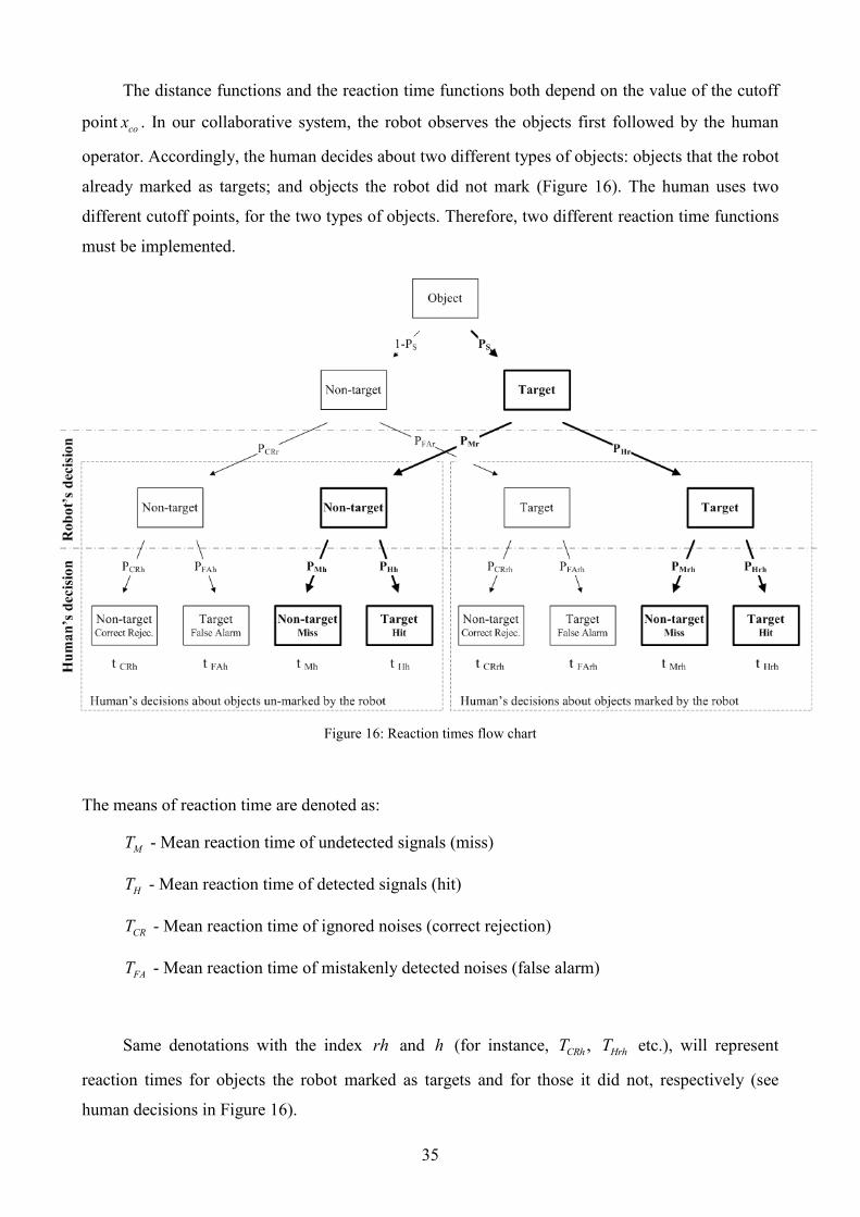
35
The distance functions and the reaction time functions both depend on the value of the cutoff
point cox . In our collaborative system, the robot observes the objects first followed by the human
operator. Accordingly, the human decides about two different types of objects: objects that the robot
already marked as targets; and objects the robot did not mark (Figure 16). The human uses two
different cutoff points, for the two types of objects. Therefore, two different reaction time functions
must be implemented.
Figure 16: Reaction times flow chart
The means of reaction time are denoted as:
MT - Mean reaction time of undetected signals (miss)
HT - Mean reaction time of detected signals (hit)
CRT - Mean reaction time of ignored noises (correct rejection)
FAT - Mean reaction time of mistakenly detected noises (false alarm)
Same denotations with the index rh and h (for instance, ,CRh HrhT T etc.), will represent
reaction times for objects the robot marked as targets and for those it did not, respectively (see
human decisions in Figure 16).

36
The equations that were developed for the normal distribution are adjusted to the signal and
noise distributions. The means and standard deviations of the signal and noise distributions are
respectively ,S S and ,N N . We used the appropriate equations (for positive or negative
responses) and parameters (mean and standard deviation of signal or noise distributions) to define
equations for mean reaction time of all four possible outcomes (miss, hit, correct rejection and false
alarm):
2 2
2 2
2 2
2 2
2
2
2
2
2
( )
( )
1 ( )
1 ( )
( )
( )
1 ( )
1 ( )
;
1( )
2
SS S
SS S
NN N
NN N
BB z
S SM
S
BB z
S SH
S
BB z
N NCR
N
BB z
N NFA
N
co S co NS N
S N
z
z BT A e
z
z BT A e
z
z BT A e
z
z BT A e
z
where
x xz z
z e
2
z
dz
When 1S N , the equations are:
2
2
2
2
2
2
2
2
( )
( )
1 ( )
1 ( )
( )
( )
1 ( )
1 ( )
S
S
N
N
BB z
SM
S
BB z
SH
S
BB z
NCR
N
BB z
NFA
N
z BT A e
z
z BT A e
z
z BT A e
z
z BT A e
z
37
4.3 Collaboration model
The basis of the expanded model developed in this thesis are the four collaboration levels
between a human operator and a robot (see subchapter 0), and the objective function that describes
the expected value of system performance (see subchapter 2.6), as developed by Bechar (2006).
The objective function of the model as described by Bechar (2006) is:
Is S Hr Hrh H C Hrh t Hr Hh H C Hh t
S Hr Hrh M Mrh t Hr Hh M Mh t
S FAr FArh FA C FArh t FAr FAh FA C FAh t
V N P [ P P (V V t V ) (1 P ) P (V V t V )]
N P [ P (1 P ) (V t V ) (1 P ) (1 P ) (V t V )]
N (1 P ) [ P P (V V t V ) (1 P ) P (V V t V )]
N
S FAr FArh CR CRrh t FAr FAh CR CRh t r t(1 P ) [ P (1 P ) (V t V ) (1 P ) (1 P ) (V t V )] t V
Each of the human time variables (denoted as Xrht or Xht ) represents a superposition of a
decision time and a motoric time (denoted as Mt ), in accordance with the collaboration level. The
decision times, previously considered as constants, are replaced with the mean reaction times
functions introduced in the previous page.
When the system operates at the R collaboration level, the robot fulfills the task all by itself
and all human time variables equal zero (there is no human intervening).
In the H collaboration level, the human does not use robot‟s help and the time variables are:
Mh Mh
Hh Hh M
CRh CRh
FAh FAh M
t T
t T t
t T
t T t
In the HR collaboration level, the robot recommends the human by indicating potential
targets. Then, the human confirms targets he thinks are real and marks extra targets the robot did
not indicate. The human does a motoric action (marking) if he thinks the robot recommended well.
The time variables are:
Mh Mh
Hh Hh M
CRh CRh
FAh FAh M
Mrh Mrh
Hrh Hrh M
CRrh CRrh
FArh FArh M
t T
t T t
t T
t T t
t T
t T t
t T
t T t
38
In the HOR collaboration level, the human supervises the robot. The robot marks targets and
the human checks those marks. The human unmarks targets that are not real and marks extra targets
that the robot missed. In this case, the human does a motoric action (unmarking) only if he thinks
the robot made a mistake. The time variables are:
Mh Mh
Hh Hh M
CRh CRh
FAh FAh M
Mrh Mrh M
Hrh Hrh
CRrh CRrh M
FArh FArh
t T
t T t
t T
t T t
t T t
t T
t T t
t T
The (motoric) time it takes to physically mark or unmark an object depends on the system
interface and the environment conditions. Therefore, it should not vary between one object to
another and it is considered as constant.

39
5 NUMERICAL ANALYSIS
A numerical analysis of the model was conducted using MatLab 7.1 (Appendix G details the
script code). The optimal cutoff points for the human and the robot were determined by numerical
computation. At the first stage, the objective function was calculated for a range of possible cutoff
points. Then, the cutoff points that yielded the highest objective function score were determined as
optimal cutoff points. The analysis of the model was performed for systems that work at the optimal
cutoff points. The objective function score was calculated for each possible combination of
parameters and variables, for each collaboration level. The best collaboration level is the level that
yields the highest objective function score for a given set of parameters‟ value.
5.1 Model parameters
The objective function of the model consists of groups of parameters that describe the task,
the environment and the observers. Table 3 introduces the parameters and their values.
5.1.1 Task types and parameters
In some systems, as mines detection or medical examinations, not to miss a target is much
more important than the cost of making false alarms. In other systems, false alarms have high cost
and the system accept to hit fewer targets in order to cause fewer false alarms. The independent
parameters of the task were determined to describe different types of tasks and systems. Raising the
gain from a hit, for example, induces the observer to make more hits at the expense of more false
alarms. The value of costs can be easily changed into any monetary values.
Analysis was focused on three types of systems: Type I system gives high priority for not
causing errors of the first type, i.e., detecting a target when a target does not exist (false alarm);
Type II system gives high priority for not causing errors of the second type, i.e., missing a target.
These two types were introduced by Oren et al. (2008). The different types of systems are
characterized by the gains and penalties for each outcome ( H M FA CRV ,V , V ,V ). For example, a high
penalty for false alarms, relatively to the other values, reduces the false alarm ratio. Similarly,
relatively high gain for hits reduces the cases of missing a target. System of Type III does not prefer
one type of error on another; therefore the values for all four possible outcomes are the same
( H M FA CRV V V V ).Table 2 details the values for each type of system.
The time cost ( TV ) is the cost of one time unit of system operation. It includes the cost of the
human operator and the robot. In order to analyze the influence of time cost regardless of the system
type, it was set relatively to the gain for a hit ( T H T H2V V V V ). The ratio between the time cost and
the gain for a hit, T H2V V , was set to the values: -80, -40, -20 (hour-1
). For example, when HV equals
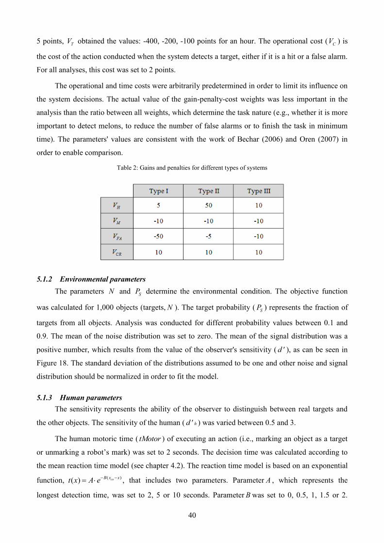
40
5 points, TV obtained the values: -400, -200, -100 points for an hour. The operational cost ( CV ) is
the cost of the action conducted when the system detects a target, either if it is a hit or a false alarm.
For all analyses, this cost was set to 2 points.
The operational and time costs were arbitrarily predetermined in order to limit its influence on
the system decisions. The actual value of the gain-penalty-cost weights was less important in the
analysis than the ratio between all weights, which determine the task nature (e.g., whether it is more
important to detect melons, to reduce the number of false alarms or to finish the task in minimum
time). The parameters' values are consistent with the work of Bechar (2006) and Oren (2007) in
order to enable comparison.
Table 2: Gains and penalties for different types of systems
5.1.2 Environmental parameters
The parameters N and SP determine the environmental condition. The objective function
was calculated for 1,000 objects (targets, N ). The target probability ( SP ) represents the fraction of
targets from all objects. Analysis was conducted for different probability values between 0.1 and
0.9. The mean of the noise distribution was set to zero. The mean of the signal distribution was a
positive number, which results from the value of the observer's sensitivity ( d ' ), as can be seen in
Figure 18. The standard deviation of the distributions assumed to be one and other noise and signal
distribution should be normalized in order to fit the model.
5.1.3 Human parameters
The sensitivity represents the ability of the observer to distinguish between real targets and
the other objects. The sensitivity of the human ( hd ' ) was varied between 0.5 and 3.
The human motoric time ( tMotor ) of executing an action (i.e., marking an object as a target
or unmarking a robot‟s mark) was set to 2 seconds. The decision time was calculated according to
the mean reaction time model (see chapter 4.2). The reaction time model is based on an exponential
function,( )
( ) coB x xt x A e
, that includes two parameters. Parameter A , which represents the
longest detection time, was set to 2, 5 or 10 seconds. Parameter B was set to 0, 0.5, 1, 1.5 or 2.

41
These values represent variety of possible exponential functions (see Figure 23). When B receives
a zero value, the mean time is A .
5.1.4 Robot parameters
The sensitivity of the robot ( rd ' ) was varied, same as human sensitivity, between 0.5 and 3.
The robot decision time ( rt ) is negligible relatively to the other times and was set to 0.01 seconds
on average for one object.
Table 3: Model parameters‟ values
5.2 Graph generator
The data included three types of systems. A record was saved for every combination of values
of the six parameters that were not constant (see Table 3). To analyze the influence of parameters
on different components of the objective function, a graph generator was developed in MatLab
(Appendix G). The application that was developed, allows to select the system type, two parameters
(X, Y) and a function (one of the components of the overall objective function), and spreads sub-
graphs for every value of third parameter. The remained three more parameters are set manually
into one of their possible values. This graph generator enabled an easy comprehensive data analysis.
Figure 17 illustrates an example of graph selection. The example describes type II system and
the function that is shown is the optimal objective function (opt_VIs). The sensitivities of the
human ( hd ' ) and the robot ( rd ' ) are varied along X and Y axes. A sub-graph is shown for every
value of the target probability ( SP ). The other three parameters ( 2B, A, vT vH ) are set manually.

42
Figure 17: Graph generator application.
The user can choose a system type (a), an objective function (b), two parameters for X and Y axes
and a third parameter for the sub graphs (c), and set manually the values of the three other parameters (d).
(a)
(b)
(d)
(c)
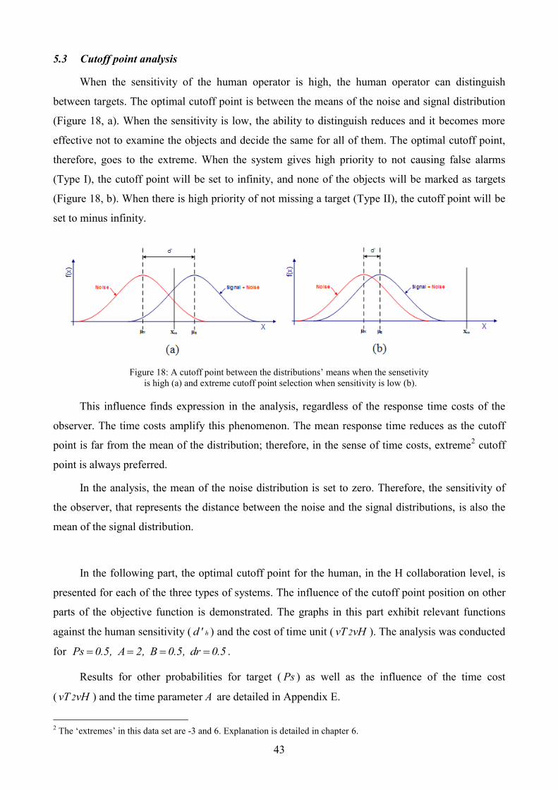
43
5.3 Cutoff point analysis
When the sensitivity of the human operator is high, the human operator can distinguish
between targets. The optimal cutoff point is between the means of the noise and signal distribution
(Figure 18, a). When the sensitivity is low, the ability to distinguish reduces and it becomes more
effective not to examine the objects and decide the same for all of them. The optimal cutoff point,
therefore, goes to the extreme. When the system gives high priority to not causing false alarms
(Type I), the cutoff point will be set to infinity, and none of the objects will be marked as targets
(Figure 18, b). When there is high priority of not missing a target (Type II), the cutoff point will be
set to minus infinity.
Figure 18: A cutoff point between the distributions‟ means when the sensetivity
is high (a) and extreme cutoff point selection when sensitivity is low (b).
This influence finds expression in the analysis, regardless of the response time costs of the
observer. The time costs amplify this phenomenon. The mean response time reduces as the cutoff
point is far from the mean of the distribution; therefore, in the sense of time costs, extreme2 cutoff
point is always preferred.
In the analysis, the mean of the noise distribution is set to zero. Therefore, the sensitivity of
the observer, that represents the distance between the noise and the signal distributions, is also the
mean of the signal distribution.
In the following part, the optimal cutoff point for the human, in the H collaboration level, is
presented for each of the three types of systems. The influence of the cutoff point position on other
parts of the objective function is demonstrated. The graphs in this part exhibit relevant functions
against the human sensitivity ( hd ' ) and the cost of time unit ( 2vT vH ). The analysis was conducted
for Ps 0.5, A 2, B 0.5, dr 0.5 .
Results for other probabilities for target ( Ps ) as well as the influence of the time cost
( 2vT vH ) and the time parameter A are detailed in Appendix E.
2 The „extremes‟ in this data set are -3 and 6. Explanation is detailed in chapter 6.
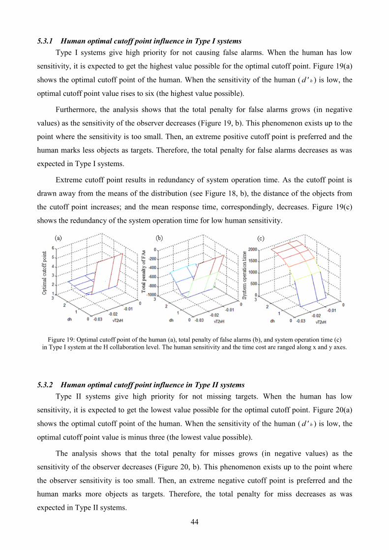
44
5.3.1 Human optimal cutoff point influence in Type I systems
Type I systems give high priority for not causing false alarms. When the human has low
sensitivity, it is expected to get the highest value possible for the optimal cutoff point. Figure 19(a)
shows the optimal cutoff point of the human. When the sensitivity of the human ( hd ' ) is low, the
optimal cutoff point value rises to six (the highest value possible).
Furthermore, the analysis shows that the total penalty for false alarms grows (in negative
values) as the sensitivity of the observer decreases (Figure 19, b). This phenomenon exists up to the
point where the sensitivity is too small. Then, an extreme positive cutoff point is preferred and the
human marks less objects as targets. Therefore, the total penalty for false alarms decreases as was
expected in Type I systems.
Extreme cutoff point results in redundancy of system operation time. As the cutoff point is
drawn away from the means of the distribution (see Figure 18, b), the distance of the objects from
the cutoff point increases; and the mean response time, correspondingly, decreases. Figure 19(c)
shows the redundancy of the system operation time for low human sensitivity.
Figure 19: Optimal cutoff point of the human (a), total penalty of false alarms (b), and system operation time (c)
in Type I system at the H collaboration level. The human sensitivity and the time cost are ranged along x and y axes.
5.3.2 Human optimal cutoff point influence in Type II systems
Type II systems give high priority for not missing targets. When the human has low
sensitivity, it is expected to get the lowest value possible for the optimal cutoff point. Figure 20(a)
shows the optimal cutoff point of the human. When the sensitivity of the human ( hd ' ) is low, the
optimal cutoff point value is minus three (the lowest value possible).
The analysis shows that the total penalty for misses grows (in negative values) as the
sensitivity of the observer decreases (Figure 20, b). This phenomenon exists up to the point where
the observer sensitivity is too small. Then, an extreme negative cutoff point is preferred and the
human marks more objects as targets. Therefore, the total penalty for miss decreases as was
expected in Type II systems.
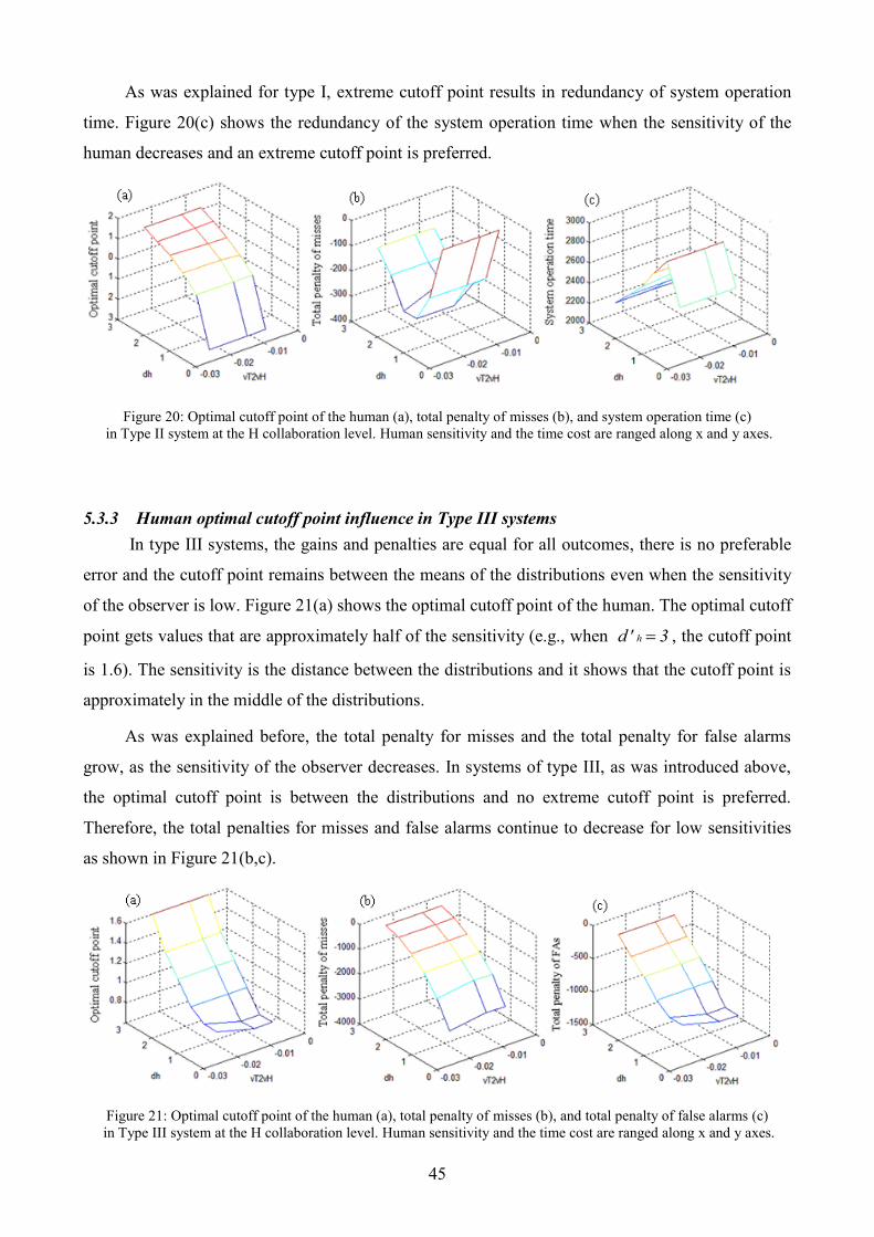
45
As was explained for type I, extreme cutoff point results in redundancy of system operation
time. Figure 20(c) shows the redundancy of the system operation time when the sensitivity of the
human decreases and an extreme cutoff point is preferred.
Figure 20: Optimal cutoff point of the human (a), total penalty of misses (b), and system operation time (c)
in Type II system at the H collaboration level. Human sensitivity and the time cost are ranged along x and y axes.
5.3.3 Human optimal cutoff point influence in Type III systems
In type III systems, the gains and penalties are equal for all outcomes, there is no preferable
error and the cutoff point remains between the means of the distributions even when the sensitivity
of the observer is low. Figure 21(a) shows the optimal cutoff point of the human. The optimal cutoff
point gets values that are approximately half of the sensitivity (e.g., when hd' 3 , the cutoff point
is 1.6). The sensitivity is the distance between the distributions and it shows that the cutoff point is
approximately in the middle of the distributions.
As was explained before, the total penalty for misses and the total penalty for false alarms
grow, as the sensitivity of the observer decreases. In systems of type III, as was introduced above,
the optimal cutoff point is between the distributions and no extreme cutoff point is preferred.
Therefore, the total penalties for misses and false alarms continue to decrease for low sensitivities
as shown in Figure 21(b,c).
Figure 21: Optimal cutoff point of the human (a), total penalty of misses (b), and total penalty of false alarms (c)
in Type III system at the H collaboration level. Human sensitivity and the time cost are ranged along x and y axes.
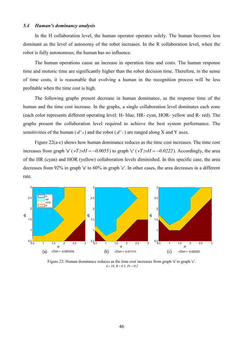
46
5.4 Human’s dominancy analysis
In the H collaboration level, the human operator operates solely. The human becomes less
dominant as the level of autonomy of the robot increases. In the R collaboration level, when the
robot is fully autonomous, the human has no influence.
The human operations cause an increase in operation time and costs. The human response
time and motoric time are significantly higher than the robot decision time. Therefore, in the sense
of time costs, it is reasonable that evolving a human in the recognition process will be less
profitable when the time cost is high.
The following graphs present decrease in human dominance, as the response time of the
human and the time cost increase. In the graphs, a single collaboration level dominates each zone
(each color represents different operating level: H- blue, HR- cyan, HOR- yellow and R- red). The
graphs present the collaboration level required to achieve the best system performance. The
sensitivities of the human ( hd ' ) and the robot ( rd ' ) are ranged along X and Y axes.
Figure 22(a-c) shows how human dominance reduces as the time cost increases. The time cost
increases from graph 'a' ( 2vT vH 0.0055 ) to graph 'c' ( 2vT vH 0.0222 ). Accordingly, the area
of the HR (cyan) and HOR (yellow) collaboration levels diminished. In this specific case, the area
decreases from 92% in graph 'a' to 60% in graph 'c'. In other cases, the area decreases in a different
rate.
Figure 22: Human dominance reduces as the time cost increases from graph 'a' to graph 'c'. A 10, B 0.5, Ps 0.2
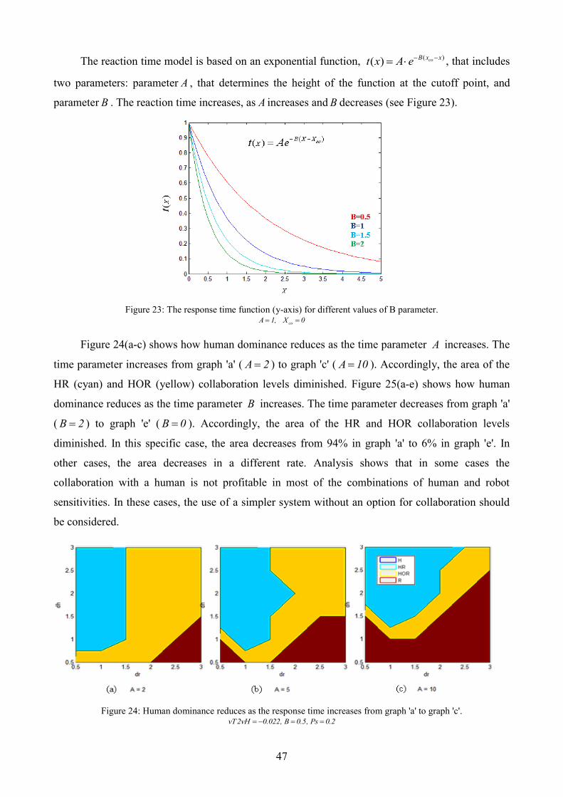
47
The reaction time model is based on an exponential function, ( )( ) coB x x
t x A e
, that includes
two parameters: parameter A , that determines the height of the function at the cutoff point, and
parameter B . The reaction time increases, as A increases and B decreases (see Figure 23).
Figure 23: The response time function (y-axis) for different values of B parameter.
coA 1, X 0
Figure 24(a-c) shows how human dominance reduces as the time parameter A increases. The
time parameter increases from graph 'a' ( A 2 ) to graph 'c' ( A 10 ). Accordingly, the area of the
HR (cyan) and HOR (yellow) collaboration levels diminished. Figure 25(a-e) shows how human
dominance reduces as the time parameter B increases. The time parameter decreases from graph 'a'
( B 2 ) to graph 'e' ( B 0 ). Accordingly, the area of the HR and HOR collaboration levels
diminished. In this specific case, the area decreases from 94% in graph 'a' to 6% in graph 'e'. In
other cases, the area decreases in a different rate. Analysis shows that in some cases the
collaboration with a human is not profitable in most of the combinations of human and robot
sensitivities. In these cases, the use of a simpler system without an option for collaboration should
be considered.
Figure 24: Human dominance reduces as the response time increases from graph 'a' to graph 'c'. vT2vH 0.022, B 0.5, Ps 0.2
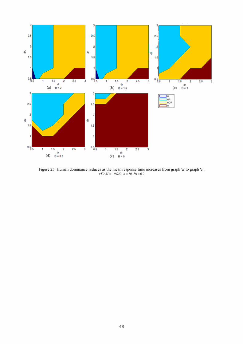
48
Figure 25: Human dominance reduces as the mean response time increases from graph 'a' to graph 'e'. vT2vH 0.022, A 10, Ps 0.2
49
6 SENSITIVITY ANALYSIS
The numerical analysis of the collaboration model was conducted for optimal cutoff points.
Sensitivity analysis of human and robot's cutoff points was performed in order to show how small
deviation from the optimal values influences the system's objective function score and the optimal
collaboration level. Specifically, we focused on the cases where small deviations from the human
optimal cutoff point cause a shift in the optimal collaboration level.
The analysis was conducted for all three cutoff points: cutoff point of the robot (XCOr) and
two cutoff points of the human for targets the robot already marked and for targets it did not mark
(XCOrh and XCOh respectively). In each case analyzed, only one cutoff point was changed.
In the analysis, the signal and noise distributions are normalized. The mean of the noise
distribution is zero and the maximum sensitivity ( rd ' or hd ' ), which is also the position of the
signal distribution mean, is three. Therefore, in order to show all possible positions, the cutoff
points' value ranged from minus three to six (i.e., three standard deviation units from the means of
the distributions).
6.1 General description and general conclusions
This section gives general description of the figures, which are shown ahead, and introduces
some common phenomena. Figure 26 is used as an example.
Each of the following figures represents a single optimal case for a given set of parameters.
One can notice that in Figure 26 there is one graph for each of the three cutoff points (XCOh, XCOrh
and XCOr from left to right). The y-axe represents the system's objective function score. In each
graph, four lines illustrate how the objective function value varies according to the change of the
cutoff point value. Each line represents one of the four collaboration levels (H-blue, HR-cyan,
HOR-yellow and R-red). A black circle marks the optimal cutoff point value on the best
collaboration level line (the highest point). In this specific case, the objective function score is 7268
and the optimal cutoff point values are XCOh=1.2, XCOrh=0.8 and XCOr=-1.6. The other parameter's
values ( dr,dh,Ps,A,B,vT2vH ) are shown in the header of the figure.
One can see that only the cutoff point of the robot affects the score of the R collaboration
level (notice straight red line in the left and middle graphs in Figure 26). Similarly, only the cutoff
point of the human, XCOh, affects the score of the H collaboration level (straight blue line in the
middle and right graphs). The scores of the HR and HOR collaboration levels are affected from all
three cutoff points.
In some cases, small deviation from the optimal cutoff point makes only a slight different in
the objective function value (notice almost straight yellow line in left graph in Figure 26). In other
50
cases, small deviation from the optimum causes a dramatic decrease of the objective function value.
If the score of the best collaboration level decreases beneath other collaboration level score, the
second level becomes the current best collaboration level (e.g., the yellow line in the middle graph
in Figure 26 decreases beneath the blue line). We denote this: a 'shift' in the best collaboration level.
In many of the analyzed cases, the optimal level yields a score that is only slightly better than
another collaboration level score. Particularly, the HR and HOR levels yield almost the same score
at the optimal cutoff points (see all following figures at this chapter).
6.2 Type III systems
6.2.1 Cutoff points analysis
6.2.1.1 Analysis of the optimal cutoff point of the robot
In all cases, a change in the value of the robot's cutoff point makes more influence on the
score of the R collaboration level than on the other levels' score. Therefore, when R is the best
collaboration level, a smaller deviation from the optimal XCOr may cause best level shifting (i.e.,
smaller than deviations from XCOr when R is not the best collaboration level).
When the best collaboration level is HR or HOR, small deviations from the optimal XCOr
usually reduce the objective function score symmetrically in both directions.
6.2.1.2 Cases where the robot is more sensitive than the human operator
In most of the cases when the robot is more sensitive than the human ( r hd' d' ), R is the
best collaboration level. In other cases, HOR is the best collaboration level but it usually has only
slightly higher score then R. For all cases, a small deviation from the optimal cutoff point does not
cause a shift in the best collaboration level.
6.2.1.3 Cases where the human operator is remarkably more sensitive than the robot
In this work, we assumed that collaboration is beneficial because the human performs better
than the robot in unstructured environments. Therefore, most of the analysis was focused on cases
where the human is more sensitive than the robot. The sensitivities of the human ( hd ' ) and the
robot ( rd ' ) were varied between 0 and 3. We denote that the human is remarkably more sensitive
than the robot in cases where h r1.5 d' d' . In cases where h r0 d' d' 1.5 we denote that, the
human is unremarkably more sensitive than the robot.
In most of the cases, when the human is remarkably more sensitive than the robot, the best
collaboration level is HR or HOR. The difference between their score, near the optimal cutoff point,
is relatively small. A small deviation from the optimal cutoff point of the human, XCOh, does not

51
cause a shift in the best collaboration level. However, a small deviation from the optimal XCOrh
enforces best level shifting to H (Figure 26).
Figure 26: Example of Type III system's score in a case where the human is remarkably more sensitive than the robot.
6.2.1.4 Cases where the human operator is unremarkably more sensitive than the robot
In most of the cases, when the human is unremarkably more sensitive than the robot
( h r0 d' d' 1.5 ), the best collaboration level is HR or HOR. The analysis reveals different
results for high, medium and low probabilities for an object to be a target ( Ps ).
Figure 27 shows one of these cases where the probability for an object to be a target is high
( Ps 0.9 ). A small deviation from the optimal cutoff point of the human, XCOh, reduces the system
score and may cause a level shifting to R. A change from the optimal value of the second cutoff
point, XCOrh, may change the best collaboration level only if the deviation is in the positive
direction. A deviation in the negative direction slightly reduces the system score but does not cause
a shift in the best collaboration level.
Figure 28 shows a case where the probability for an object to be a target is low ( Ps 0.1 ). In
this case, a small deviation from the optimal XCOh, may change the best collaboration level only if
the deviation is in the negative direction. A deviation in the positive direction slightly reduces the
system score but does not cause a shift in the best collaboration level. A change from the optimal
value XCOrh, reduces the system score and may cause level shifting.
Figure 29 shows a case where the probability for an object to be a target is medium
( Ps 0.5 ). A small deviation from optimal XCOh, in the negative direction may change the best
collaboration level. On the other hand, a small deviation in the positive direction reduces the system
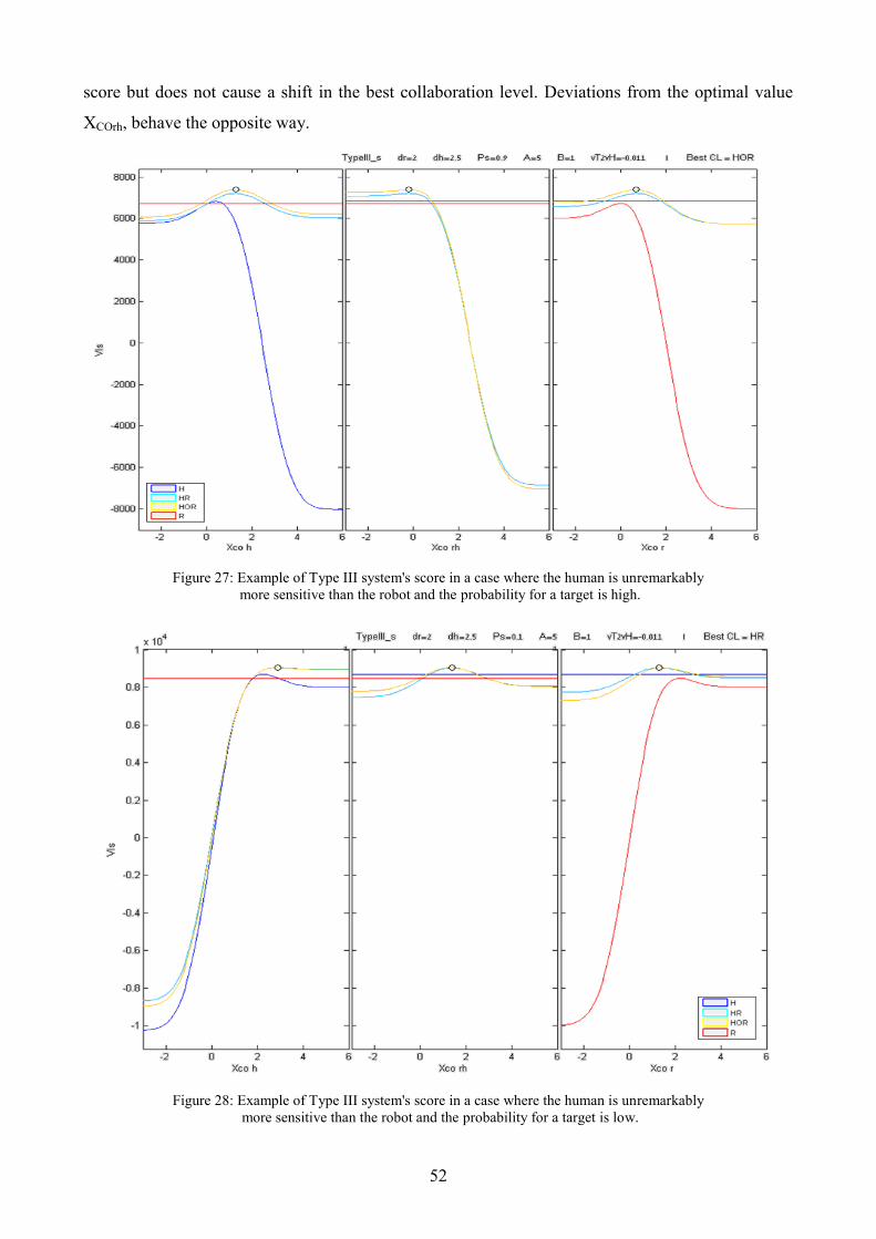
52
score but does not cause a shift in the best collaboration level. Deviations from the optimal value
XCOrh, behave the opposite way.
Figure 27: Example of Type III system's score in a case where the human is unremarkably
more sensitive than the robot and the probability for a target is high.
Figure 28: Example of Type III system's score in a case where the human is unremarkably
more sensitive than the robot and the probability for a target is low.
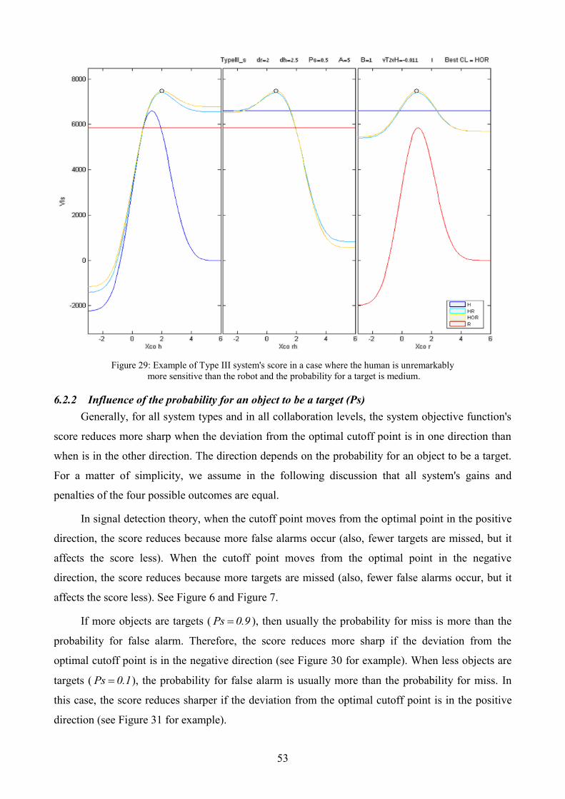
53
Figure 29: Example of Type III system's score in a case where the human is unremarkably
more sensitive than the robot and the probability for a target is medium.
6.2.2 Influence of the probability for an object to be a target (Ps)
Generally, for all system types and in all collaboration levels, the system objective function's
score reduces more sharp when the deviation from the optimal cutoff point is in one direction than
when is in the other direction. The direction depends on the probability for an object to be a target.
For a matter of simplicity, we assume in the following discussion that all system's gains and
penalties of the four possible outcomes are equal.
In signal detection theory, when the cutoff point moves from the optimal point in the positive
direction, the score reduces because more false alarms occur (also, fewer targets are missed, but it
affects the score less). When the cutoff point moves from the optimal point in the negative
direction, the score reduces because more targets are missed (also, fewer false alarms occur, but it
affects the score less). See Figure 6 and Figure 7.
If more objects are targets ( Ps 0.9 ), then usually the probability for miss is more than the
probability for false alarm. Therefore, the score reduces more sharp if the deviation from the
optimal cutoff point is in the negative direction (see Figure 30 for example). When less objects are
targets ( Ps 0.1 ), the probability for false alarm is usually more than the probability for miss. In
this case, the score reduces sharper if the deviation from the optimal cutoff point is in the positive
direction (see Figure 31 for example).
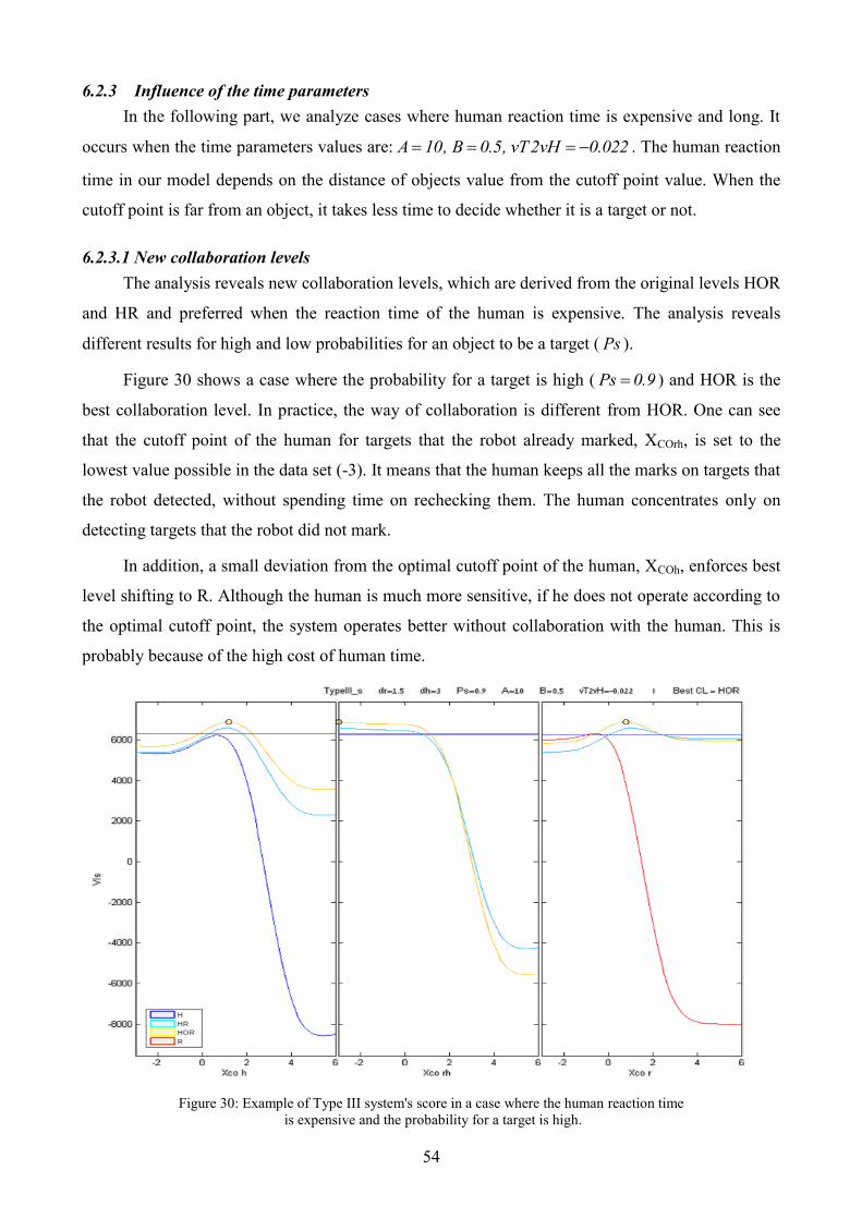
54
6.2.3 Influence of the time parameters
In the following part, we analyze cases where human reaction time is expensive and long. It
occurs when the time parameters values are: A 10, B 0.5, vT2vH 0.022 . The human reaction
time in our model depends on the distance of objects value from the cutoff point value. When the
cutoff point is far from an object, it takes less time to decide whether it is a target or not.
6.2.3.1 New collaboration levels
The analysis reveals new collaboration levels, which are derived from the original levels HOR
and HR and preferred when the reaction time of the human is expensive. The analysis reveals
different results for high and low probabilities for an object to be a target ( Ps ).
Figure 30 shows a case where the probability for a target is high ( Ps 0.9 ) and HOR is the
best collaboration level. In practice, the way of collaboration is different from HOR. One can see
that the cutoff point of the human for targets that the robot already marked, XCOrh, is set to the
lowest value possible in the data set (-3). It means that the human keeps all the marks on targets that
the robot detected, without spending time on rechecking them. The human concentrates only on
detecting targets that the robot did not mark.
In addition, a small deviation from the optimal cutoff point of the human, XCOh, enforces best
level shifting to R. Although the human is much more sensitive, if he does not operate according to
the optimal cutoff point, the system operates better without collaboration with the human. This is
probably because of the high cost of human time.
Figure 30: Example of Type III system's score in a case where the human reaction time
is expensive and the probability for a target is high.
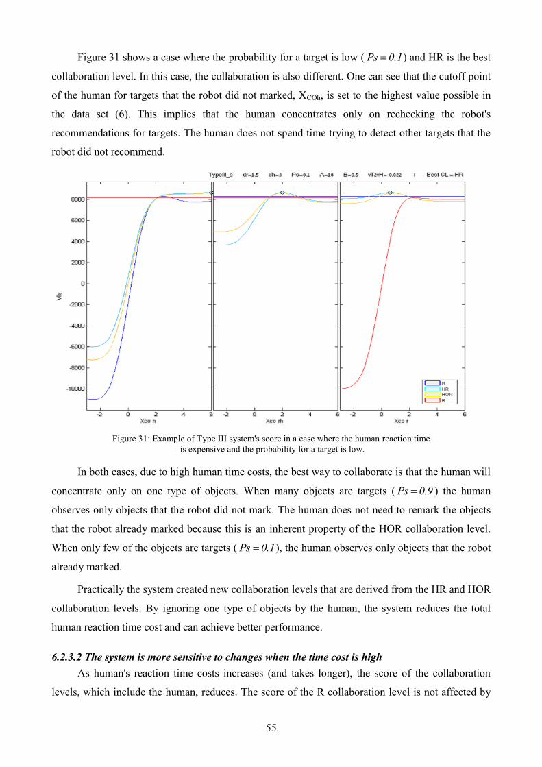
55
Figure 31 shows a case where the probability for a target is low ( Ps 0.1 ) and HR is the best
collaboration level. In this case, the collaboration is also different. One can see that the cutoff point
of the human for targets that the robot did not marked, XCOh, is set to the highest value possible in
the data set (6). This implies that the human concentrates only on rechecking the robot's
recommendations for targets. The human does not spend time trying to detect other targets that the
robot did not recommend.
Figure 31: Example of Type III system's score in a case where the human reaction time
is expensive and the probability for a target is low.
In both cases, due to high human time costs, the best way to collaborate is that the human will
concentrate only on one type of objects. When many objects are targets ( Ps 0.9 ) the human
observes only objects that the robot did not mark. The human does not need to remark the objects
that the robot already marked because this is an inherent property of the HOR collaboration level.
When only few of the objects are targets ( Ps 0.1 ), the human observes only objects that the robot
already marked.
Practically the system created new collaboration levels that are derived from the HR and HOR
collaboration levels. By ignoring one type of objects by the human, the system reduces the total
human reaction time cost and can achieve better performance.
6.2.3.2 The system is more sensitive to changes when the time cost is high
As human's reaction time costs increases (and takes longer), the score of the collaboration
levels, which include the human, reduces. The score of the R collaboration level is not affected by
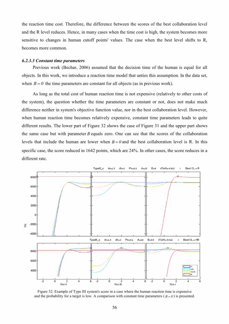
56
the reaction time cost. Therefore, the difference between the scores of the best collaboration level
and the R level reduces. Hence, in many cases when the time cost is high, the system becomes more
sensitive to changes in human cutoff points' values. The case when the best level shifts to R,
becomes more common.
6.2.3.3 Constant time parameters
Previous work (Bechar, 2006) assumed that the decision time of the human is equal for all
objects. In this work, we introduce a reaction time model that unties this assumption. In the data set,
when B 0 the time parameters are constant for all objects (as in previous work).
As long as the total cost of human reaction time is not expensive (relatively to other costs of
the system), the question whether the time parameters are constant or not, does not make much
difference neither in system's objective function value, nor in the best collaboration level. However,
when human reaction time becomes relatively expensive, constant time parameters leads to quite
different results. The lower part of Figure 32 shows the case of Figure 31 and the upper part shows
the same case but with parameter B equals zero. One can see that the scores of the collaboration
levels that include the human are lower when B 0 and the best collaboration level is R. In this
specific case, the score reduced in 1642 points, which are 24%. In other cases, the score reduces in a
different rate.
Figure 32: Example of Type III system's score in a case where the human reaction time is expensive
and the probability for a target is low. A comparison with constant time parameters ( B 0 ) is presented.
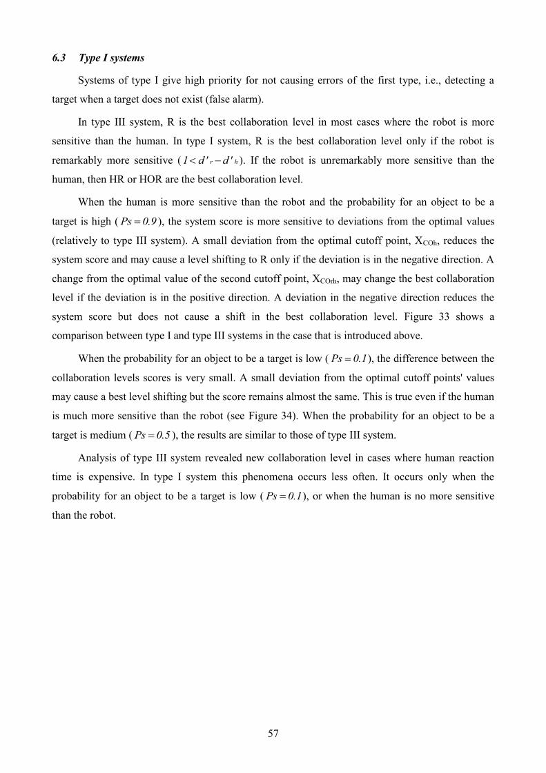
57
6.3 Type I systems
Systems of type I give high priority for not causing errors of the first type, i.e., detecting a
target when a target does not exist (false alarm).
In type III system, R is the best collaboration level in most cases where the robot is more
sensitive than the human. In type I system, R is the best collaboration level only if the robot is
remarkably more sensitive ( r h1 d' d' ). If the robot is unremarkably more sensitive than the
human, then HR or HOR are the best collaboration level.
When the human is more sensitive than the robot and the probability for an object to be a
target is high ( Ps 0.9 ), the system score is more sensitive to deviations from the optimal values
(relatively to type III system). A small deviation from the optimal cutoff point, XCOh, reduces the
system score and may cause a level shifting to R only if the deviation is in the negative direction. A
change from the optimal value of the second cutoff point, XCOrh, may change the best collaboration
level if the deviation is in the positive direction. A deviation in the negative direction reduces the
system score but does not cause a shift in the best collaboration level. Figure 33 shows a
comparison between type I and type III systems in the case that is introduced above.
When the probability for an object to be a target is low ( Ps 0.1 ), the difference between the
collaboration levels scores is very small. A small deviation from the optimal cutoff points' values
may cause a best level shifting but the score remains almost the same. This is true even if the human
is much more sensitive than the robot (see Figure 34). When the probability for an object to be a
target is medium ( Ps 0.5 ), the results are similar to those of type III system.
Analysis of type III system revealed new collaboration level in cases where human reaction
time is expensive. In type I system this phenomena occurs less often. It occurs only when the
probability for an object to be a target is low ( Ps 0.1 ), or when the human is no more sensitive
than the robot.

58
Figure 33: Comparison between Type I and Type III systems' score in a case where
the human is more sensitive than the robot and the probability for a target is high.
Figure 34: Example of Type I system's score in a case where the probability
for a target is low and the difference between the collaboration levels scores is small.
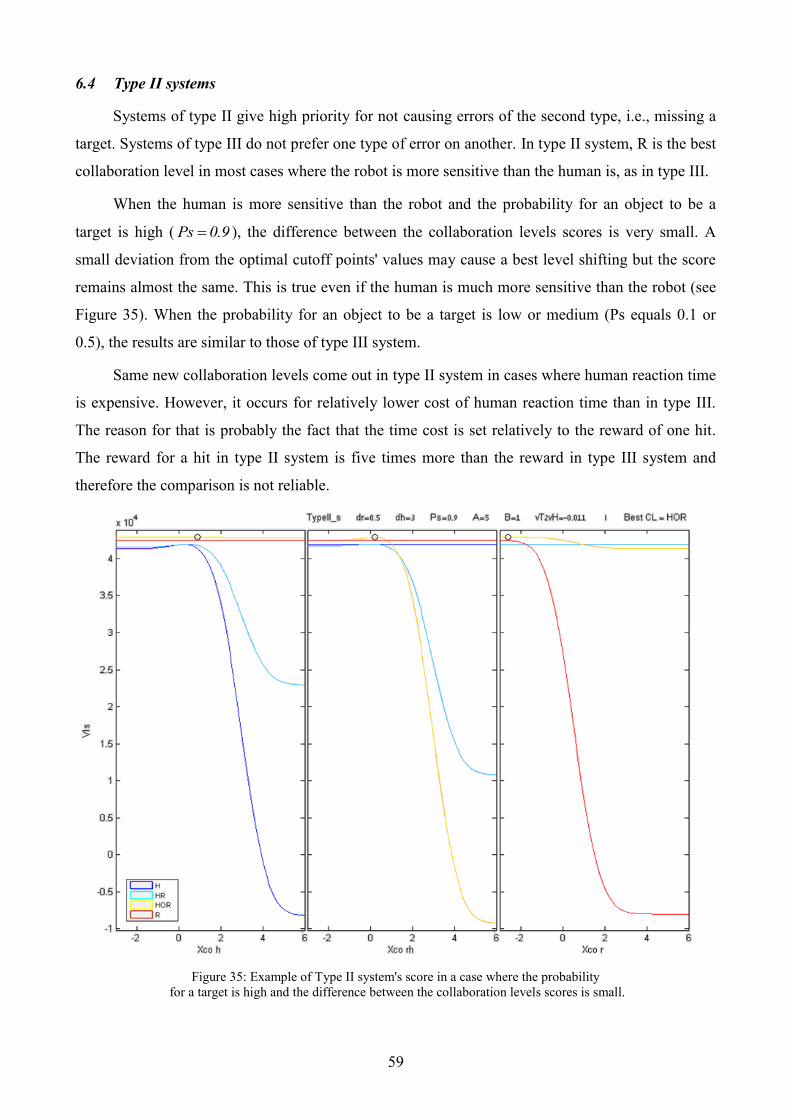
59
6.4 Type II systems
Systems of type II give high priority for not causing errors of the second type, i.e., missing a
target. Systems of type III do not prefer one type of error on another. In type II system, R is the best
collaboration level in most cases where the robot is more sensitive than the human is, as in type III.
When the human is more sensitive than the robot and the probability for an object to be a
target is high ( Ps 0.9 ), the difference between the collaboration levels scores is very small. A
small deviation from the optimal cutoff points' values may cause a best level shifting but the score
remains almost the same. This is true even if the human is much more sensitive than the robot (see
Figure 35). When the probability for an object to be a target is low or medium (Ps equals 0.1 or
0.5), the results are similar to those of type III system.
Same new collaboration levels come out in type II system in cases where human reaction time
is expensive. However, it occurs for relatively lower cost of human reaction time than in type III.
The reason for that is probably the fact that the time cost is set relatively to the reward of one hit.
The reward for a hit in type II system is five times more than the reward in type III system and
therefore the comparison is not reliable.
Figure 35: Example of Type II system's score in a case where the probability
for a target is high and the difference between the collaboration levels scores is small.

60
61
7 CONCLUSIONS AND FUTURE RESEARCH
7.1 Conclusions
Bechar (2006) developed a model for evaluating performance of human-robot collaborative
target recognition systems. This work introduces further development of the model by incorporating
non-constant reaction times. The new model, proposed in this research, might describe actual
systems in a better way by adjusting time parameters to a specific task and taking into consideration
the fact that reaction time of the human depends on the strength of the observed object. Evaluating
the best collaboration level according to the new model, considers the influence of human reaction
time on system performance.
The analysis revealed additional collaboration levels, which are derived from the HR and
HOR collaboration levels defined in Bechar‟s work (Bechar, 2006), and are the best collaboration
level when human time costs are high. In these collaboration levels, the human concentrates only on
one type of objects. When many objects are targets, the human observes only objects that the robot
did not mark and does not check objects that the robot marked (based on the HOR collaboration
level). When only few of the objects are targets, the human observes only objects that the robot
recommended and does not try to detect other targets (based on the HR collaboration level). Since
the human ignores one type of objects, the system reduces the total human reaction time cost and
can achieve better performance.
The human ignores objects by setting his/her cutoff point to an extreme value. When the
cutoff point is the highest positive value possible, none of the objects is higher than the cutoff point
so none of them is marked as a target. Similarly, when the cutoff point value is the lowest possible,
all the objects are marked as targets. The analysis shows how the system type, the human
sensitivity, the probability of an object to be a target, and the time cost all influence the phenomena
of extreme cutoff point selection.
When the human sensitivity is low, the human badly discriminates between targets and other
objects. If the system gives high priority for not causing false alarms (type I systems), the human
prefers an extreme positive cutoff point, resulting in no objects that are marked as targets, and no
false alarms. For systems that give high priority for not missing targets (type II systems), an
extreme negative cutoff point was preferred, resulting in all objects marked as targets and no
misses.
The probability of an object to be a target ( Ps ) influences this phenomenon. In type II
systems, when there are many targets among the objects (i.e., Ps is high), the system prefers
extreme cutoff point for higher sensitivities of the human (relatively to low sensitivities in cases

62
where Ps is not high and an extreme cutoff point is preferred). In a similar manner, when most of
the objects are not targets (i.e., Ps is low), in type I systems, an extreme cutoff point is preferred
for higher sensitivities of the human. A reasonable explanation for this influence is the potential of
misses or false alarms to occur. When there are many targets, the potential of missing a target is
higher; and when there are few targets, the potential of false alarms is high.
The analysis shows that mean reaction time and time costs affect the position of the optimal
cutoff point. The phenomenon, introduced above, arises for higher human sensitivities as the mean
time and/or the time cost are higher. Furthermore, the analysis shows that collaboration with a
human is less profitable in cases when the time cost is high. In these cases, the R collaboration
level, that does not include a human, is the optimal collaboration level.
An extreme cutoff point position decreases the total operation time cost. The mean response
time reduces as the cutoff point is far from the mean of the distribution; therefore, in the sense of
time costs, the extreme cutoff point is always preferred.
The position of the cutoff point influences all other parts of the objective function. An
extreme positive cutoff point, for example, causes small probabilities of false alarms and hits; and
causes high probabilities of miss and correct rejections. The overall gains and penalties of these
outcomes are modified accordingly.
7.2 Research limitations
It must be noted that although this research includes an in-depth analysis of the new objective
function, it was impossible to analyze and investigate all possible variables' combinations due to the
multitude of variables that are involved. Hence, the thesis presents the most common trends and the
conclusions are limited to the analyzed cases.
Furthermore, the results are strongly linked to the analyzed cases because of the high
dependency on the many parameters. Therefore, we presented only trends and did not detail
quantitative results, which are specific and highly depend on the chosen parameters.
This work focused only on the optimal collaboration level. In some cases, the optimal level
yields a score that is only slightly better than another collaboration level score. In addition,
switching the level of operation during the task is related to some operational costs. Hence, it might
not always be worthy to operate at the best level. The analysis and conclusions are therefore limited
also in this aspect.

63
7.3 Definition of the new collaboration levels
The research discovered a phenomenon, in which the human ignores objects by setting his
cutoff point to an extreme value. An in-depth analysis of this phenomenon revealed two new
collaboration levels, which are derived from the HR and the HOR collaboration levels defined in
Bechar‟s work (Bechar, 2006), and are the best collaboration level when the human time cost is
high. In each of the new collaboration levels, the human observes only one type of objects and
ignores another. The new collaboration levels can be defined as follows.
HR2: The human operator observes only objects that the robot recommended to mark as
targets. The human acknowledges the robot‟s correct detections and ignores recommendations that
are false alarms. The human operator cannot mark other targets, which the robot did not
recommend.
HOR2: Targets are identified and marked automatically by the robot‟s detection algorithm
and the human operator cannot change these marks. The human operator assignment is to detect and
mark the targets missed by the robot.
7.4 Future research
The following directions are worthy future investigation:
7.4.1 Determination of the Reaction time type: constant versus variable
This research analyzes the influence of human reaction time in human robot collaborative
systems. Different aspects of the influence were discussed, but one question remained unanswered:
When is it essential to regard reaction time as a variable, while designing or analyzing a system, and
when can it be considered as constant? One of the three terms should occur in order to determine
reaction time as a constant: 1) when the contribution of the reaction time part to the objective
function is small relative to the other parts; 2) the difference between the objective function scores
when using reaction time as a variable or a constant is small; and 3) when the involvement of the
human operation is small. In some cases, considering constant time parameters will most likely
produce a good estimation of system performance. However, in other cases, e.g., when the cost of
system operation time is high, modeling reaction time is probably essential. Future research should
answer this question and differentiate between those cases.
64
7.4.2 New/additional collaboration levels
The analysis revealed two new collaboration levels and future research should investigate
these further. These collaboration levels are derived from the HR and HOR collaboration levels by
adjusting one of the human cutoff points to extreme positive or negative value. In practice, although
the optimal cutoff point should make the human concentrate only on one type of objects, the human
might not operate optimally and therefore, might spend time and efforts on the other type of objects.
Systems that officially include these two new collaboration levels as part of other levels may
perform better. Future research should investigate in what cases these collaboration levels are the
best collaboration level.
7.4.3 Experiment of human reaction time influence
This work included a preliminary analysis of human reaction time based on data acquired in
an experiment conducted by Bechar (2006). Bechar (2006) conducted an experiment simulating
melon detection in order to examine the influence of different human-robot collaboration levels in a
target recognition task. During the experiment, all human operations were recorded. In this work,
we analyzed experimental data, focusing on the human reaction time and regarding them as
variables. We showed the relation between image complexity and decision time of the human
operator (see Appendix H). However, since this work was very limited in scope it is included only
as an Appendix.
An experiment of target recognition, specially designed to examine human reaction time,
should check how time pressure on the subjects influences their performance. It can also discover
how well the reaction time model of Murdock (1985) and other models, describe reaction time.
7.4.4 Examination of different reaction time models
This research used a reaction time model based on Murdock (1985). Other models describe
reaction time differently. Future research can examine other models and validate them with
experiments. The examination can discover how the influence of human reaction time depends on
the reaction time model; and what phenomena do not depend on the models.
7.4.5 Analytical development of an optimal cutoff point
The new model, proposed in this research, includes a reaction time function that depends on
the cutoff point position. Signal detection theory does not apply to this time function, and therefore,
the optimal cutoff point that the theory supply must be adjusted. A further study may provide
analytical development of the new optimal cutoff point. One must calculate a derivative of the
objective function in order to find the cutoff point results in the maximum value.
65
7.4.6 Use of mean distances to evaluate mean reaction times
This study includes analytical development of the mean distance model, which calculates the
mean distance between the cutoff point and objects of the same category (e.g., mean distance of all
objects that were 'missed'). Future research can investigate the use of the mean distance model to
evaluate mean time.
7.4.7 Collaboration level switching
This work focused only on the optimal collaboration level. Future research should apply full
system optimization, which should consider the cost of switching between levels (Takach, 2008)
and not only the cost of operating at the best collaboration level.
7.4.8 Collaboration in other stages of human information processing
Parasuraman et al. (2000) introduce a four-stage model of human information processing (see
subchapter 0). The four stages in the model are: (1) information acquisition, (2) information
analysis, (3) decision and action selection, and (4) action implementation. In this thesis, we
introduce a collaboration model only for the decision and action selection stage. Future work should
investigate levels of collaboration for the other stages.
7.4.9 Additional analysis
Due to the multitude variables in the model, there are numerous combinations and cases to
analyze. This thesis presents the most common trends and additional analyses are required.

66
67
8 REFERENCES
Bechar, A., J. Meyer and Y. Edan (2009). An Objective Function to Evaluate Performance of
Human-Robot Collaboration in Target Recognition Tasks. IEEE Transactions on Systems,
Man and Cybernetics, Part C (In press).
Bechar A. (2006). Human-Robot Collaboration Methods for Target Recognition in Unstructured
Environments. Ph.D. dissertation, Industrial Engineering and Management, Ben-Gurion
University of the Negev, Beer-Sheva, Israel.
Bechar A. & Edan Y. (2003). Human-Robot Collaboration for Improved Target Recognition of
Agricultural Robots. Industrial Robot 30(5): 432-436.
Bechar A. & Edan Y. (2000). Human-Robot Collaboration for Agricultural Robot Guidance. ASAE
Paper No. 00-3135. ASAE, St. Joseph, MI.
Bhanu B., Jones G., Lin Y.Q. & Peng J. (2000). Adaptive Target Recognition. Machine Vision and
Applications 11(6): 289-299.
Brown C.D. & Davis H.T. (2006). Receiver Operating Characteristics Curves and Related Decision
Measures: A Tutorial. Chemometrics and Intelligent Laboratory Systems 80(1): 24-38.
Bruemmer D.J., Boring R.A., Few D. A., Marble J.A., Nielsen C.W. and Walton M.C. (2005).
Shared Understanding for Collaborative Control. IEEE Transactions on Systems, Man and
Cybernetics: Part A, vol. 35, no. 4, pp. 494-504.
Bulanon D.M., Hiroma T., Kataoka T., Ota, Y. and Zhang S. (2001). Optimal Thresholding for the
Automatic Recognition of Apple Fruits. ASAE Paper No. 01-3133. ASAE, St. Joseph, MI.
Burke J. L., Lumelsky V. J., Murphy R. R., Rogers E. and Scholtz J. (2004). Final Report for the
DARPA/NSF Interdisciplinary Study on Human–Robot Interaction. IEEE Transactions on
Systems, Man and Cybernetics: Part C, vol. 34, no. 2, pp. 103–112.
Cohen H. & Ferrell W. R. (1969). Human Operator Decision-Making in Manual Control. IEEE
Transactions on Man-Machine Systems. Vol. MMS-10, no. 2, pp. 41-53.
Czarnecki C. & Graves A.R. (2000). Design Patterns for Behavior-Based Robotics. IEEE
Transactions on Systems, Man and Cybernetics: Part A, vol. 30, no. 1, pp. 36-41.
Dubey R. & Everett S. (1998). Human-Machine Cooperative Telerobotics Using Uncertain Sensor
and Model Data. Proceedings of the IEEE International Conference on Robotics and
Automation. Leuven, Belgium. pp. 1615-1622.
Hughes S.B. & Lewis M. (2005). Task-Driven Camera Operations for Robotic Exploration. IEEE
Transactions on Systems, Man and Cybernetics: Part A, vol. 35, no. 4, pp. 513-522.
http://wise.cgu.edu. Signal Detection Theory Tutorial. Retrieved November 2007, from World
Wide Web: http://wise.cgu.edu/sdtmod/index.asp
68
Murdock B. B. & Dufty P. O. (1972). Strength Theory and Recognition Memory. Journal of
Experimental Psychology, vol. 94, No. 3, pp. 284-290.
Murdock B. B. (1985). An analysis of the strength-latency relationship. Memory and Cognition, 13
(6), 511-521.
Obuchowski N.A. (2003). Receiver Operating Characteristic Curves and Their Use in Radiology.
Radiology 229 3– 8.
Oren Y. (2007). Performance Analysis of Human-Robot Collaboration in Target Recognition Tasks.
B.Sc dissertation, Industrial Engineering and Management, Ben-Gurion University of the
Negev, Beer-Sheva, Israel.
Oren Y., Bechar A., Joachim M., Edan Y. (2008). Performance Analysis of Human-Robot
Collaboration in Target Recognition Tasks. IEEE International Conference on Distributed
Human-Machine Systems. Athens, Greece.
Parasuraman R., Sheridan T.B. and Wickens C.D. (2000). A Model for Types and Levels of Human
Interaction with Automation. IEEE Transactions on Systems, Man and Cybernetics: part A,
vol. 30, no. 3, pp. 286-197.
Pike R. (1973). Response Latency Models for Signal Detection. Psychological Review, vol. 80, No.
1, pp. 53-68.
Ratcliff R. & Rouder J. F. (1998). Modeling Response Times for Two Choice Decisions.
Psychological Science, vol. 9, No. 5, pp. 347-356.
Ratcliff R., Mckoon G., and Zandt T. V. (1999). Connectionist and Diffusion Models of Reaction
Time. Psychological Review, vol. 106, No. 2, pp. 261-300.
Ratcliff R. & Smith P. L. (2004). A Comparison of Sequential Sampling Models for Two-Choice
Reaction Time. Psychological Review, vol. 111, No. 2, pp. 333-367.
Rodriguez G. & Weisbin C.R. (2003). A New Method to Evaluate Human-Robot System
Performance. Autonomous Robots 14: 165–178.
Sheridan T.B. & Verplank W.L. (1978). Human and Computer Control of Undersea Teleoperators.
MIT Man-Machine Systems Laboratory. Cambridge, MA, Tech. Rep.
Sheridan T.B. (1992). Telerobotics, Automation and Supervisory Control. Cambridge, MA. MIT.
Steinfeld A. (2004). Interface Lessons for Fully and Semi-Autonomous Mobile Robots.
Proceedings of the IEEE International Conference on Robotics and Automation, 3.
Takach I. (2008). Switching between collaboration levels in target recognition tasks. M.Sc.
dissertation, Industrial Engineering and Management, Ben-Gurion University of the Negev,
Beer-Sheva, Israel.
Welford A. T. (1980). Reaction Times. London, Academic Press.
Wickens T. D. (2002). Elementary Signal Detection Theory. New York, Oxford University. Press.
69
9 APPENDIXES
APPENDIX A - NORMAL, STANDARD NORMAL, SIGNAL AND NOISE DISTRIBUTIONS ...................... 70
1. Normal distribution ................................................................................................................. 70
2. Standard normal distribution ................................................................................................... 70
3. The relation between normal and standard normal distributions ............................................ 71
4. Signal distribution ................................................................................................................... 72
5. Noise distribution .................................................................................................................... 72
APPENDIX B - EXPRESSION OF Z AS A FUNCTION OF BETA AND D’ (BECHAR, 2006) ..................... 73
APPENDIX C - VALIDATION OF MEAN DISTANCE EQUATIONS ........................................................ 74
APPENDIX D - DEVELOPMENT OF MEAN REACTION TIME .............................................................. 75
1. Mean reaction time of negative responses .............................................................................. 76
2. Mean reaction time of positive responses ............................................................................... 79
APPENDIX E - NUMERICAL ANALYSIS - ADDITIONAL RESULTS ...................................................... 82
1. Type I analysis ........................................................................................................................ 82
2. Type II analysis ....................................................................................................................... 82
3. Type III analysis...................................................................................................................... 82
4. Time influence on the optimal cutoff point position ............................................................... 86
APPENDIX F - PAPER FOR THE 20TH
INTERNATIONAL CONFERENCE ON PRODUCTION RESEARCH
............................................................................................................................................................ 87
APPENDIX G - THE NUMERIC SIMULATION SOFTWARE .................................................................. 93
1. The experiment program code ................................................................................................ 93
2. The data base creator code ...................................................................................................... 94
3. The graph generator code ...................................................................................................... 100
4. The mean time function ........................................................................................................ 105
APPENDIX H - THE RELATION BETWEEN IMAGE COMPLEXITY AND REACTION TIME ................ 107
1. Melon detection experiment .................................................................................................. 107
2. Data preparation .................................................................................................................... 108
3. Results ................................................................................................................................... 109
APPENDIX I - RAW DATA OF THE EXPERIMENT ............................................................................. 112
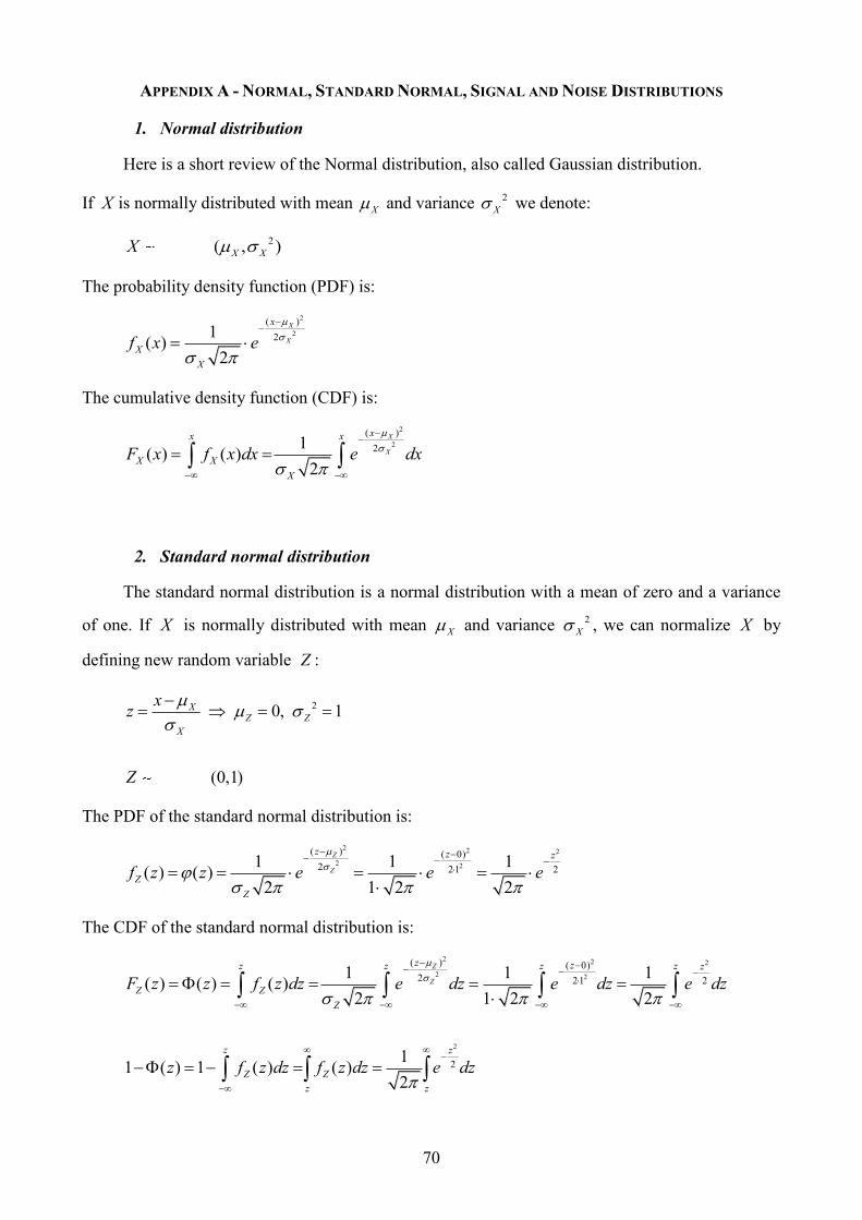
70
APPENDIX A - NORMAL, STANDARD NORMAL, SIGNAL AND NOISE DISTRIBUTIONS
1. Normal distribution
Here is a short review of the Normal distribution, also called Gaussian distribution.
If X is normally distributed with mean X and variance 2
X we denote:
2( , )X XX Normal
The probability density function (PDF) is:
2
2
( )
21( )
2
X
X
x
X
X
f x e
The cumulative density function (CDF) is:
2
2
( )
21( ) ( )
2
X
X
xx x
X X
X
F x f x dx e dx
2. Standard normal distribution
The standard normal distribution is a normal distribution with a mean of zero and a variance
of one. If X is normally distributed with mean X and variance 2
X , we can normalize X by
defining new random variable Z :
20, 1
(0,1)
XZ Z
X
xz
Z Normal
The PDF of the standard normal distribution is:
2 2 2
2 2
( ) ( 0)
2 2 1 21 1 1
( ) ( )2 1 2 2
Z
Z
z z z
Z
Z
f z z e e e
The CDF of the standard normal distribution is:
2 2 2
2 2
2
( ) ( 0)
2 2 1 2
2
1 1 1( ) ( ) ( )
2 1 2 2
11 ( ) 1 ( ) ( )
2
Z
Z
z zz z z z z
Z Z
Z
z z
Z Z
z z
F z z f z dz e dz e dz e dz
z f z dz f z dz e dz

71
3. The relation between normal and standard normal distributions
Here is an interpretation of the link between the normal distribution and the standard normal
distribution. If X is normally distributed, then for a specific value cox we can define coz , a specific
value of the random variable Z which is standard normal distributed.
co Xco
X
xz
The PDF of X can be defined, using the PDF of Z :
22
2
( )
2 21 1 1 1
( ) ( )2 2
1( ) ( )
co Xco
X
x z
X co co
X XX
X co co
X
f x e e z
f x z
The CDF of X can be defined, using the CDF of Z :
21( )
21( ) ( )
2
:
( )
1
Xco co
X
xx x
X co X
X
XX X
X
X XX X
X
X
co Xco co
X
X
F x f x dx e dx
Changing the domain of integration
xz x z
d zdxdx dz
dz dz
x z
xx x z z
2
2
2
z
Xe
2
21
( )2
( ) ( )
co coz z z
co
X co co
dz e dz z
F x z
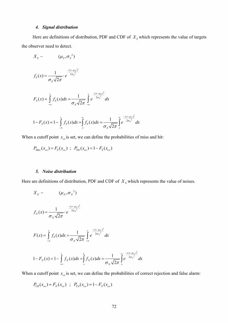
72
4. Signal distribution
Here are definitions of distribution, PDF and CDF of SX which represents the value of targets
the observer need to detect.
2
2
2
2
2
2
2
( )
2
( )
2
( )
2
( , )
1( )
2
1( ) ( )
2
11 ( ) 1 ( ) ( )
2
S
S
S
S
S
S
S S S
x
S
S
xx x
S S
S
xx
S S S
x xS
X Normal
f x e
F x f x dx e dx
F x f x dx f x dx e dx
When a cutoff point cox is set, we can define the probabilities of miss and hit:
( ) ( ) ; ( ) 1 ( )Miss co S co Hit co S coP x F x P x F x
5. Noise distribution
Here are definitions of distribution, PDF and CDF of NX which represents the value of noises.
2
2
2
2
2
2
2
( )
2
( )
2
( )
2
( , )
1( )
2
1( ) ( )
2
11 ( ) 1 ( ) ( )
2
N
N
N
N
N
N
N N N
x
N
N
xx x
S
N
xx
N N N
x xN
X Normal
f x e
F x f x dx e dx
F x f x dx f x dx e dx
When a cutoff point cox is set, we can define the probabilities of correct rejection and false alarm:
( ) ( ) ; ( ) 1 ( )CR co N co FA co N coP x F x P x F x
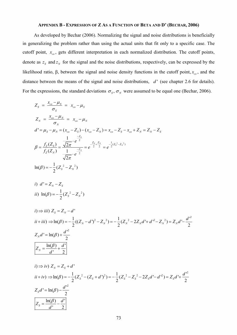
73
APPENDIX B - EXPRESSION OF Z AS A FUNCTION OF BETA AND D’ (BECHAR, 2006)
As developed by Bechar (2006). Normalizing the signal and noise distributions is beneficially
in generalizing the problem rather than using the actual units that fit only to a specific case. The
cutoff point, cox , gets different interpretation in each normalized distribution. The cutoff points,
denote as Sz and Nz for the signal and the noise distributions, respectively, can be expressed by the
likelihood ratio, β, between the signal and noise density functions in the cutoff point, cox , and the
distance between the means of the signal and noise distributions,
'd (see chapter 2.6 for details).
For the expressions, the standard deviations ,S N were assumed to be equal one (Bechar, 2006).
2 2
21
( )2 2 2
2
2 2
2 2
' ( ) ( )
1
( ) 2
( ) 1
2
1ln( ) ( )
2
) '
1) ln( ) ( )
2
) )
S
S NS N
N
co SS co S
S
co NN co N
N
S N co S co N co S co N N S
Z
Z ZZ Z
Z S
Z
Z N
S N
N S
S N
S N
xZ x
xZ x
d x Z x Z x Z x Z Z Z
ef Z
e ef Z
e
Z Z
i d Z Z
ii Z Z
i iii Z Z
22 2 2 2 2
2
22 2 2 2 2
2
'
1 1 ') ln( ) (( ') ) ( 2 ' ' ) '
2 2 2
'' ln( )
2
ln( ) '
' 2
) ) '
1 1 ') ln( ) ( ( ') ) ( 2 ' ' ) '
2 2 2
'' ln( )
2
ln( )
'
N N N N N N
N
N
N S
S S S S S S
S
S
d
dii iii Z d Z Z Z d d Z Z d
dZ d
dZ
d
i iv Z Z d
dii iv Z Z d Z Z Z d d Z d
dZ d
dZ
d
'
2
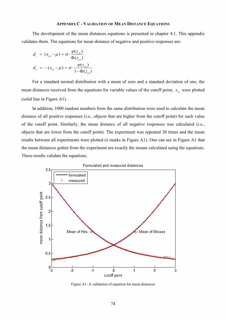
74
APPENDIX C - VALIDATION OF MEAN DISTANCE EQUATIONS
The development of the mean distances equations is presented in chapter 4.1. This appendix
validates them. The equations for mean distance of negative and positive responses are:
( )( )
( )
( )( )
1 ( )
coco
co
coco
co
zd x
z
zd x
z
For a standard normal distribution with a mean of zero and a standard deviation of one, the
mean distances received from the equations for variable values of the cutoff point, cox were plotted
(solid line in Figure A1).
In addition, 1000 random numbers from the same distribution were used to calculate the mean
distance of all positive responses (i.e., objects that are higher from the cutoff point) for each value
of the cutoff point. Similarly, the mean distance of all negative responses was calculated (i.e.,
objects that are lower from the cutoff point). The experiment was repeated 30 times and the mean
results between all experiments were plotted (x marks in Figure A1). One can see in Figure A1 that
the mean distances gotten from the experiment are exactly the means calculated using the equations.
These results validate the equations.
Figure A1: A validation of equation for mean distances
75
APPENDIX D - DEVELOPMENT OF MEAN REACTION TIME
The development of mean reaction time is based on Murdock (1985). Different denotations
for the parameters of the exponential function ( ,A B ) and for the cutoff point ( cox ) is the only
difference from Murdock‟s model. An exponential function is used in order to transfer the strength
of an object into the reaction time of the observer. Strength of an object is its distance from the
cutoff point.
For negative responses, the distance and the reaction time functions are:
( )
( )
( ) co
co
B x x
d x x x
t x A e
For positive responses the distance and the reaction time functions are:
( )
( )
( ) co
co
B x x
d x x x
t x A e
Mean reaction times of negative and positive responses depend on the cutoff point and are
denoted respectively as ( ), ( )co coT x T x .
76
1. Mean reaction time of negative responses
In order to find the mean reaction time of negative responses, one must calculate weighted
average of all reaction times (results from x-values) of objects with a value lower than the cutoff
point. The weights are the frequencies of x.
2
2
2
2
( )
( )
2
( )
( ) 2
( ) ( )
( )
( )
( )
( )
:
1( )
2
( ) ( )
1
2
( )
co
co
co
co
co
co
co
co
co
x
co x
x
B x x
x
x
x
co
x x
B x x
co
B x B
t x f x dx
T x
f x dx
A e f x dx
f x dx
From the normal distribution
f x e
f x dx F x
A e e dx
F x
A e e
2
2
2
2
2
2
( )
2
( )
2
( )
2
1
2
( )
1
2
( )
1
2
( )
co
co
co
co
co
x x
x
co
x x
B x
B x
co
x xB x
B x
co
e dx
F x
e e dx
A eF x
e dx
A eF x
77
2
2
2 2
2
2 2 2
2
2 2 2
2
1 ( )( 2 )
2
1 2 ( )
2
2 2
2
2 2
2
1
2
( )
1
2
( )
1
2
( )
1
2
co
co
co
co
co
co
co
x xB x
B x
co
x B x x
B x
co
x B x x x
B x
co
B x x x
B x
e dx
A eF x
e dx
A eF x
e dx
A eF x
e e
A e
2
2 2
2
2
2
2 2 2 2 2 2
2
2
2
2 2 2
2
2
2
2
2 ( )
2
2
2 ( ) ( ) ( )
2
2
( ) 2 (
2
2
( )
1
2
( )
1
2
( )
1
2
co
co
co
co
co
co
x
co
x x x B
B x
co
x x x B B B
B x
co
B x x
B x
dx
F x
e dx
A e eF x
e dx
A eF x
e e
A e
2 2 2
2
2 2 2 2
2
2 2 2
2 2
2 2
2
2 2 2
2 2
2
2
) ( )
2
2 ( ) ( )
2( )
2 2
( ( ))
2( )
2 2
2
( )
1
2
( )
1
2
( )
co
co
co
co
co
co
x B B
co
x x x B B
BB x
co
x x B
BB x
co
B x
dx
F x
e dx
A e eF x
e dx
A eF x
A e
2 2
2
2 2 2 4
2
2
( ( ))
22
2
1
2
( )
co
co
x x B
B B
co
B x
e dx
F x
A e
22
2
2
2B
2 2
2 2 2B
22
2 2
2
( ( ))
21
2
( )
cox x B
co
e dx
F x

78
2 2
2
2 2
22
2 2
( ( ))
2
2
1 ( )( )
2
( )2
22
2
1
2
( )
1
2
( )
:
( )
( )
co
co
co
co
x x B
BB x B
co
x x B
BB x
co
e dx
A eF x
e dx
A eF x
Changing the domain of integration
x Bu x B u
dx d B udx
du du
2 2
2
2
( )2
( )
( )
1
co
coco co
BB x
du
Bx u
x Bx x u u
A e
2
2
2
u
e
2
2 2
2 2
2
2
2
( )2
2
2
( )
:
( )1( ) ( )
2
( )( )
( )
(
co
co
co
co
u
co
u u
coco
coB
B x
co
cox B
B
du
F x
From the standard normal distribution
x Be du u
x B
A eF x
x B
A e
2 2
2 2
2
2
2
2
)
( )
:
; ( ) ( ) ( )
( )
( )
( )( )
( )
1( )
2
1
co
co
co
co coco co co
BB z
co
co
BB z
coco
co
coco
z z
where
F x
From the standard normal distribution
x xz F x z
z BA e
z
z BT x A e
z
xz
z e dz
if then
T
2
2( )
( )( )
co
BB z
coco
co
z Bx A e
z
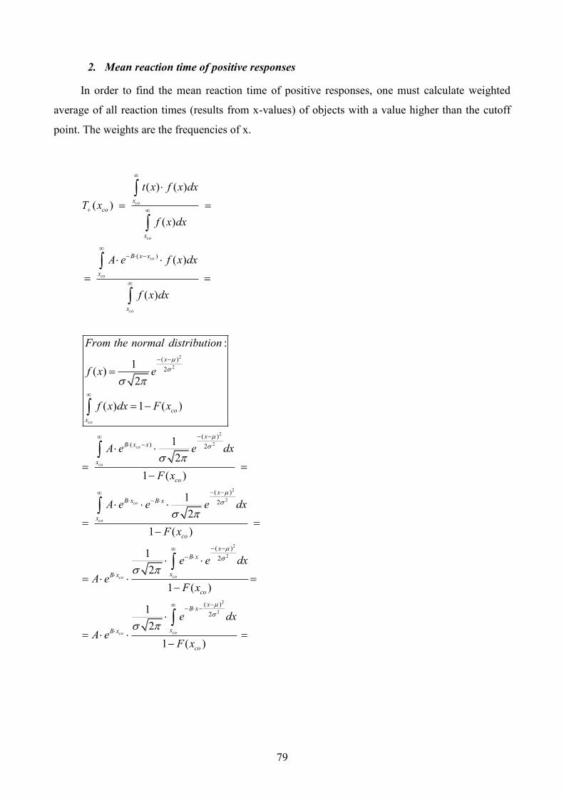
79
2. Mean reaction time of positive responses
In order to find the mean reaction time of positive responses, one must calculate weighted
average of all reaction times (results from x-values) of objects with a value higher than the cutoff
point. The weights are the frequencies of x.
2
2
2
2
( )
( )
2
( )
( ) 2
( ) ( )
( )
( )
( )
( )
:
1( )
2
( ) 1 ( )
1
2
1 ( )
co
co
co
co
co
co
co
co
co
x
co
x
B x x
x
x
x
co
x
x
B x x
x
co
B x B x
t x f x dx
T x
f x dx
A e f x dx
f x dx
From the normal distribution
f x e
f x dx F x
A e e dx
F x
A e e
2
2
2
2
2
2
( )
2
( )
2
( )
2
1
2
1 ( )
1
2
1 ( )
1
2
1 ( )
co
coco
coco
x
x
co
x
B x
xB x
co
xB x
xB x
co
e dx
F x
e e dx
A eF x
e dx
A eF x
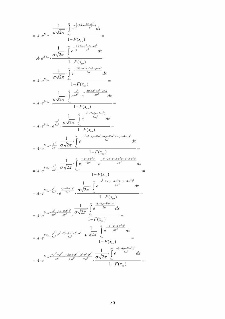
80
2
2
2 2
2
2 2 2
2
2 2 2
2 2
1 ( )(2 )
2
1 2 ( )
2
2 2
2
2 2
2 2
1
2
1 ( )
1
2
1 ( )
1
2
1 ( )
1
2
coco
coco
coco
co
xB x
xB x
co
B x x
xB x
co
B x x x
xB x
co
B x x x
B x
e dx
A eF x
e dx
A eF x
e dx
A eF x
e e d
A e
2 2
2
2
2
2 2 2 2 2 2
2
2
2
2 2 2
2
2
2
2 ( )
2
2
2 ( ) ( ) ( )
2
2
( ) 2 (
2
2
1 ( )
1
2
1 ( )
1
2
1 ( )
1
2
co
S
coco
coco
co
x
co
x x B
xB x
co
x x B B B
B xx
co
B x x B
B x
x
F x
e dx
A e eF x
e dx
A eF x
e e
A e
2 2 2
2
2 2 2 2
2
2 2 2
2 2
2 2
2
2 2 2
2 2
2 2
2
) ( )
2
2 ( ) ( )
2
( )
2 2
( ( ))
2
( )
2 2
2
2
1 ( )
1
2
1 ( )
1
2
1 ( )
co
coco
coco
co
B
x
co
x x B B
BB x
x
co
x B
BB x
x
co
B x
dx
F x
e dx
A e eF x
e dx
A eF x
A e
2 2
2
2 2 4
2
2
( ( ))
2
2
1
2
1 ( )
co
co
x B
B Bx
co
B x
e dx
F x
A e
22
2
2
2B
2 2
2 2 2B
22
2 2
2
( ( ))
21
2
1 ( )
co
x B
x
co
e dx
F x
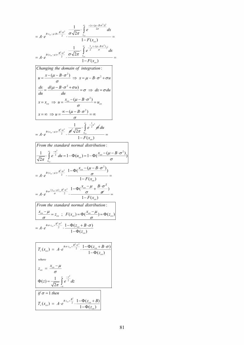
81
2 2
2 2
22
2 2
( ( ))
2
2
1 ( )( )
2
( )2
22
2
1
2
1 ( )
1
2
1 ( )
:
( )
( )
coco
coco
x B
BB x B x
co
x B
BB x x
co
e dx
A eF x
e dx
A eF x
Changing the domain of integration
x Bu x B u
dx d B udx
du du
2 2
2
2
( )2
( )
( )
1
co
coco co
BB x
du
x Bx x u u
Bx u
A e
21
2
2
u
e
2
2 2
2 2
2
2
2
( )2
2
( )
2
1 ( )
:
( )11 ( ) 1 ( )
2
( )1 ( )
1 ( )
1 ( )
1 ( )
co
co
co
co
u
co
u
coco
u
coB
B x
co
cox B
B
co
du
F x
From the standard normal distribution
x Be du u
x B
A eF x
x B
A eF x
From the s
2 2
2 2
2
2
2
2
:
; ( ) ( ) ( )
1 ( )
1 ( )
1 ( )( )
1 ( )
1( )
2
1
( )
co
co
co coco co co
BB z
co
co
BB z
coco
co
coco
z z
B
co
where
tandard normal distribution
x xz F x z
z BA e
z
z BT x A e
z
xz
z e dz
if then
T x A e
2
21 ( )
1 ( )
co
Bz
co
co
z B
z
82
APPENDIX E - NUMERICAL ANALYSIS - ADDITIONAL RESULTS
In the following part, the optimal cutoff point of the human in the H collaboration level is
analyzed for each of the three types of systems. The graphs in this part exhibit the cutoff point
against the human sensitivity ( hd ' ) and the cost of time unit ( 2vT vH ), for each value of the time
parameter ( A ). The analysis was conducted for B 0.5, dr 0.5 .
Figure A2 - Figure A4 show the graphs for systems of type I - III, respectively. Each figure
shows graphs for different probabilities of object to be target ( Ps 0.1, 0.2, 0.5, 0.8, 0.9 )
1. Type I analysis
Type I systems give high priority for not causing false alarms. Figure A2 shows the optimal
cutoff point (z-axis) of the human for different probabilities of targets ( Ps ). When Ps is 0.1
(Figure A2-a), an extreme positive cutoff point is preferred for relatively high sensitivities
( hd' 1.5 ). As Ps increases to 0.5 (Figure A2-c), i.e., half of the objects are targets, the system
prefers an extreme cutoff point only for lower sensitivities ( hd' 0.5 ). As Ps increases further to
0.8, 0.9 (Figure A2-d,e), i.e., most of the objects are targets, the system does not prefer an extreme
cutoff point.
2. Type II analysis
Type II systems give high priority for not missing targets. Figure A3 shows the optimal cutoff
point (z-axis) of the human for different probabilities of targets ( Ps ). When Ps is high, 0.9 (Figure
A3-e), an extreme negative cutoff point is preferred for relatively high sensitivities ( hd' 2.5 ).
As Ps decreases to 0.5 (Figure A3-c), the system prefers an extreme cutoff point only for lower
sensitivities ( hd' 1 ). As Ps decreases further to 0.2, 0.1 (Figure A3-b,a), i.e., most of the objects
are not targets, the system prefers an extreme positive cutoff point for low sensitivities ( hd' 1 ).
3. Type III analysis
Type III systems do not prefer one type of error on the other. Figure A4 shows the optimal
cutoff point (z-axis) of the human for different probabilities of targets ( Ps ). When Ps is 0.5,
(Figure A4-c), the optimal cutoff point value is approximately half of the human sensitivity, which
represents the distance between the means of the distributions (i.e., the cutoff point is between the
means of the distributions). When Ps decreases to 0.2, 0.1 (Figure A4-a,b), the system prefers an
extreme positive cutoff point for low sensitivities ( hd' 0.5 1.5 ). When Ps increases to 0.8, 0.9
(Figure A4-d,e), the system prefers an extreme negative cutoff point for low sensitivities
( hd' 0.5 1 ).
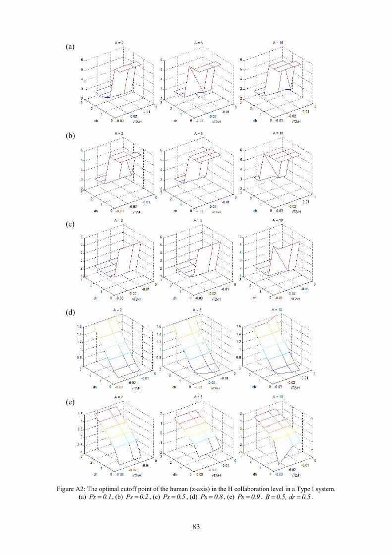
83
Figure A2: The optimal cutoff point of the human (z-axis) in the H collaboration level in a Type I system.
(a) Ps 0.1 , (b) Ps 0.2 , (c) Ps 0.5 , (d) Ps 0.8 , (e) Ps 0.9 . B 0.5, dr 0.5 .
(a)
(b)
(c)
(d)
(e)
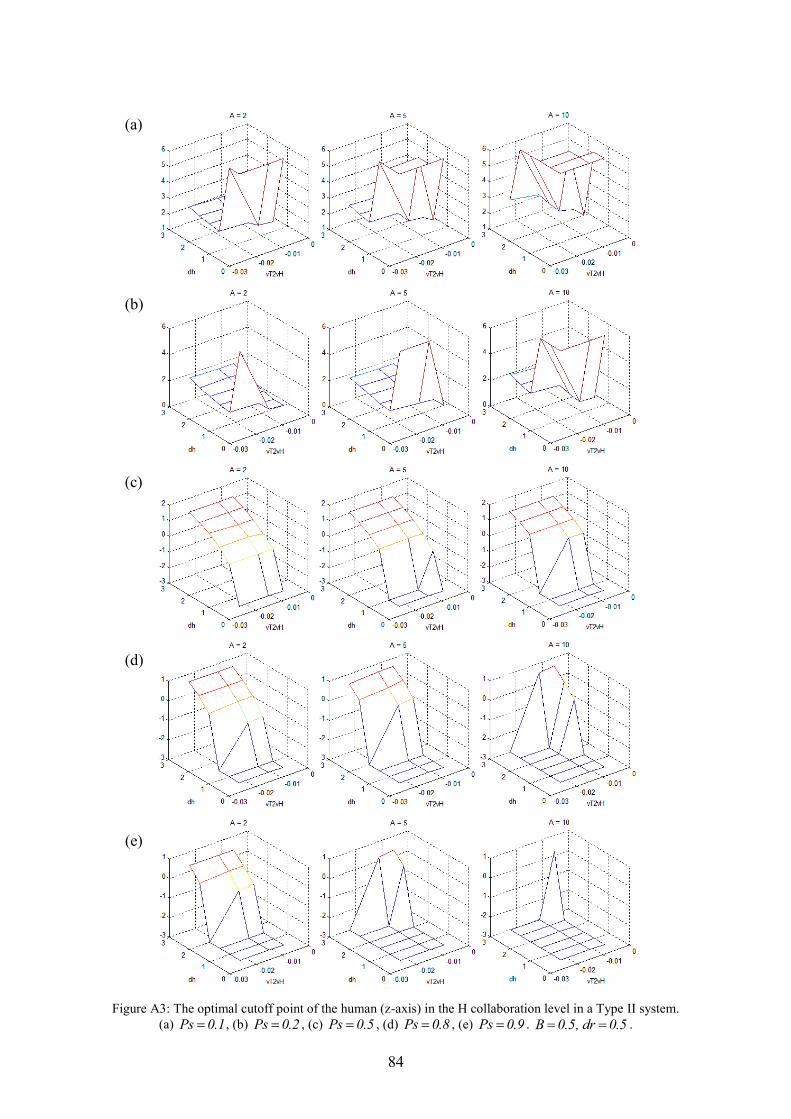
84
Figure A3: The optimal cutoff point of the human (z-axis) in the H collaboration level in a Type II system.
(a) Ps 0.1 , (b) Ps 0.2 , (c) Ps 0.5 , (d) Ps 0.8 , (e) Ps 0.9 . B 0.5, dr 0.5 .
(a)
(b)
(c)
(d)
(e)
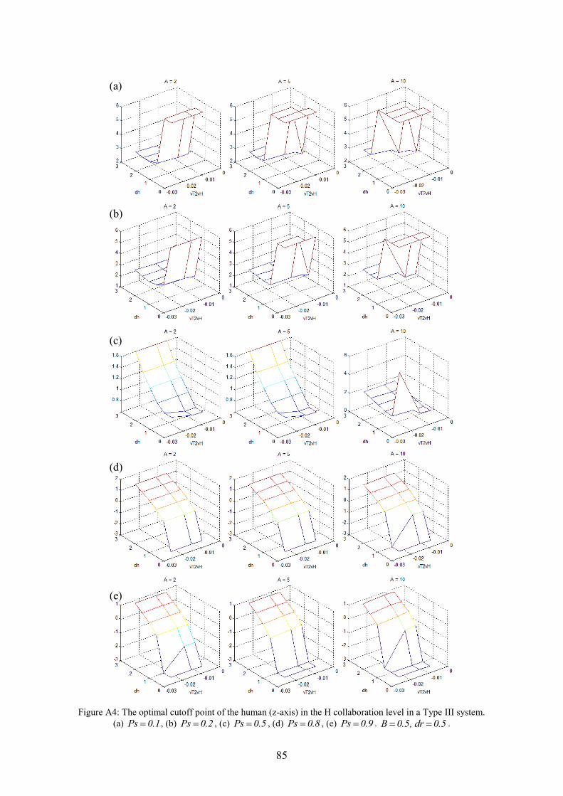
85
Figure A4: The optimal cutoff point of the human (z-axis) in the H collaboration level in a Type III system.
(a) Ps 0.1 , (b) Ps 0.2 , (c) Ps 0.5 , (d) Ps 0.8 , (e) Ps 0.9 . B 0.5, dr 0.5 .
(a)
(b)
(c)
(d)
(e)

86
4. Time influence on the optimal cutoff point position
An extreme cutoff point position decreases the total operation time cost. The mean reaction
time reduces as the cutoff point is far from the mean of the distribution; therefore, in the sense of
time costs, extreme cutoff point is always preferred.
In all the graphs (Figure A2 - Figure A4), the cutoff point varies with the change of the time
cost ( 2vT vH ) along X-axis. When the time cost is high, an extreme cutoff point is preferred for
higher human sensitivities. For example, see the left graph in Figure A4-a. When the time cost is
high ( 2vT vH 0.03 ), an extreme cutoff point (z value is 6) is preferred for human sensitivities
that are less than two ( hd' 2 ). However, when the time cost is low ( 2vT vH 0.01 ), an
extreme cutoff point (6) is preferred only for human sensitivities that are less than one ( hd' 1 ).
Parameter A is coordinated with mean reaction time of the human (i.e., high mean reaction
time is expected when A holds high values) and has the same influence. Parameter A equals two on
the left graphs and increases to ten on the right graphs. An extreme cutoff point is preferred for
higher human sensitivities as parameter A increases. For example, see Figure A4-a. In the left graph
A 2 and an extreme cutoff point (6) is preferred only for human sensitivities that are less than one
( hd' 1 ). As parameter A increases to 5 or 10 (in the other two graphs), an extreme cutoff point
(6) is preferred also for higher human sensitivities.
To conclude, the analysis shows that parameter A and time cost affect the position of the
optimal cutoff point. The phenomenon, of extreme cutoff point position, arises for higher human
sensitivities as parameter A and/or the time cost are higher.

87
APPENDIX F - PAPER FOR THE 20TH
INTERNATIONAL CONFERENCE ON PRODUCTION RESEARCH
INFLUENCE OF HUMAN REACTION TIME ON PERFORMANCE OF HUMAN-ROBOT
TARGET RECOGNITION SYSTEMS
D. Yashpe
1, A. Bechar
2 and Y. Edan
1
1Department of Industrial Engineering and Management, Ben-Gurion University of the Negev, Beer-Sheva, Israel
2Institute of Agricultural Engineering, Agricultural Research Organization - Volcani Center, Bet-Dagan, Israel
Abstract
This study aims to evaluate the influence of human‟s reaction time on performance of integrated human-robot target recognition. Particularly, the study presents a model to evaluate the effect of reaction time on the human-robot collaboration level. The model‟s objective function quantifies the influence of robot, human, environment and task parameters, through a weighted sum of performance measures. Simulation analysis considered reaction time that depended on the signal strength of the observed object. Results reveal an extreme threshold selection, in two cases: when human sensitivity reduces, and when the cost of time increases. An extreme threshold selection decreases the total operational time costs.
Keywords:
Human-robot collaboration, collaboration levels, reaction time, target recognition.
1 INTRODUCTION
Autonomous robots are systems that can perform tasks without human intervention. They are best suited for applications that require accuracy and high yield under stable conditions, yet they lack the capability to respond to unknown, changing and unpredicted events [1]. Humans, dissimilarly, can easily fit themselves into changing unstructured environment and undefined targets [1]. By taking advantage of the human perception skills and the robot's accuracy and consistency, the combined human-robotic system can be simplified, resulting in improved performance [1].
In human-robot collaborative systems, types of collaboration levels differ by nature, scale, structure, and number of levels. Sheridan [2] describes ten levels of automation of decision and action selection. Bechar and Edan [3] evaluate two collaboration levels for agriculture robot guidance through an off-road path. Bruemmer et al. [4] determine four modes of control of a remote mobile robot in an in-door search and exploration task. Hughes and Lewis [5] use two different levels of control on robot‟s cameras in order to control it in a remote environment. Czarnecki and Graves [6] describe a scale of five human-robot interaction levels for a telerobotic behavior based system.
Target recognition is a critical element in most robotic systems [1] including industrial and service applications, quality assurance, medical, agriculture and remote sensing [1]. Automatic target recognition in unstructured outdoor environments is characterized by low detection rates and high false alarm rates [7].
Reaction time is the cognitive time required for the observer to decide whether an object is a target or not. Accuracy in target recognition measures the ability of the observer to detect targets correctly. The relation between reaction time and accuracy varies according to whether speed or accuracy of performance is emphasized; and according to whether one response or another is more probable or weighted more heavily [8]. Murdock [9] analyses the strength-latency relationship and introduces a generic reaction time model based on the distance-from-
criteria of the observed object. He suggests that an exponential function is the most reasonable to use in order to transfer the object‟s strength, i.e., distance-from-criteria, into latency. In this research, a reaction time model, based on Murdock [9], is incorporated into Bechar‟s [1] collaboration model.
The study aims to evaluate the influence of human‟s reaction time on the performance of an integrated human-robot system, designated for target recognition tasks. Particularly, the study focuses on how reaction time affects the level of human- robot collaboration that results in best performance.
2 METHODOLOGY
2.1 Collaboration levels
Four collaboration levels for target recognition were designed based on [1]: i) H - the Human, unaided, detects and marks the desired target; ii) HR - the Human marks targets, aided by recommendations from an automatic detection algorithm, i.e., the targets are automatically marked by a Robot detection algorithm, the human acknowledges the robot‟s correct detections, ignores false detections and marks targets missed by the robot; iii) HOR - the Human Operators' assignment is to cancel false detections and to mark the targets missed by an automatic Robot detection algorithm; and iv) R - the targets are marked automatically by the system (Robot).
2.2 Collaboration model
The collaboration model was based on a model defined in [1]. An objective function describes the expected value of system performance, given the properties of the environment and the system. The goal is to maximize the objective function. The objective function (VIs, equation 1) is composed of the four responses of the target detection process and the system operational costs:
Is Hs Ms FAs CRs TsV V V V V V (1)
Where VHs is the gain for target detections (hits), VFAs is the penalty for false alarms, VMs is the system penalty for missing targets, VCRs is the gain for correct rejections, and VTs is the system operation cost. All gain, penalty and cost values have the same units, which enable us to add them

88
together to a single value, expressed in the objective function. The gain and penalty functions are:
Hs S Hs HV N P P V (2)
Ms S Ms MV N P P V (3)
1 FAs S FAs FAV N ( P ) P V (4)
1 CRs S CRs CRV N ( P ) P V (5)
Where, N is the number of objects in the observed image and PS is the probability of an object becoming a target. The third parameter in the equations, PXs, is the system
probability for one of the outcomes: hit, miss, false alarm or correct rejection (X can be H, M, FA and CR). The fourth parameter, VX, is the system gain or penalty from an expected outcome.
The system‟s probability of a certain outcome is influenced by the serial structure of the model and is composed of the robot and the human probabilities:
1 Hs Hr Hrh Hr Hh( )P P P P P (6)
1 Ms Mr Mh Mr Mrh( )P P P P P (7)
1 FAs FAr FArh FAr FAh( )P P P P P (8)
1 CRs CRr CRh CRr CRrh( )P P P P P (9)
Where:
PHr is the robot probability of a hit, PHrh is the probability of confirming a robot hit and PHh is the human probability of detecting a target that the robot did not detect;
PMr is the robot miss probability, PMrh is the human probability of not confirming a robot hit and PMh is the human probability of missing a target the robot missed. PFAr is the robot false alarm probability, PFArh is the human probability of not avoiding a robot false alarm and PFAh is
the human probability of a false alarm on targets the robot correctly rejected;
PCRr is the robot probability of a correct rejection, PCRrh is the human probability of correcting a robot false alarm and PCRh is the human probability of a correct rejection on targets the robot correctly rejected.
The sum of hit and miss probabilities (of the same type) and the sum of false alarm and correct rejection probabilities equals one.
The system‟s operation cost is:
1 Ts S t S Hs S FAs CV t V [N P P N ( P ) P ] V (10)
Where, tS is the time required by the system to perform a task, Vt is the cost of one time unit, and VC is the operation cost of one object recognition (hit or false alarm).
The system time consists of the time it takes the human to decide whether to confirm or reject robot detections; and the time it takes the human to decide whether objects not detected by the robot are targets or not. The robot operation time of processing the images and performing hits or false alarms, is also included.
1
1
1 1
1
1 1
1 1
1 1
S S Hr Hrh Hrh
S Hr Hh Hh
S Hr Hrh Mrh
S Hr Hh Mh
S FAr FArh FArh
S FAr FAh FAh
S FAr FArh CRrh
S FAr
t N P P P t
N P ( P ) P t
N P P ( P ) t
N P ( P ) ( P ) t
N ( P ) P P t
N ( P ) ( P ) P t
N ( P ) P ( P ) t
N ( P ) ( P ) 1 FAh CRh r( P ) t N t
(11)
Where:
tHrh is the human time required to confirm a robot hit and tHh is the human time required to hit a target that the robot did not hit;
tMrh is the human time lost when a robot hit is missed and tMh is the human time invested when missing a target that
the robot did not hit;
tFArh is the human time needed not to avoid a robot false alarm and tFAh is the human false alarm time;
tCRrh is the human time to correctly reject a robot false alarm, tCRh is the human correct rejection time, and tr is the robot operation time.
Explicit operation of the system objective function, VIs, which is suitable for all collaboration levels, is:
1
1
1 1
1
1
Is S Hr Hrh H C Hrh t
Hr Hh H C Hh t
S Hr Hrh M Mrh t
Hr Hh M Mh t
S FAr FArh FA C FArh t
FAr FAh FA C FAh t
V N P [ P P (V V t V )
( P ) P (V V t V )]
N P [ P ( P ) (V t V )
( P ) ( P ) (V t V )]
N ( P ) [ P P (V V t V )
( P ) P (V V t V )]
1 1
1 1
S FAr FArh CR CRrh t
FAr FAh CR CRh t r t
N ( P ) [ P ( P ) (V t V )
( P ) ( P ) (V t V )] N t V
(12)
For the H collaboration level, the system objective function will be a degenerate form of the full objective function, and will not include the robot variables:
1
1
1
Is S Hh H C Hh t
Hh M Mh t
S FAh FA C FAh t
FAh CR CRh t
V N P [ P (V V t V )
( P ) (V t V )]
N ( P ) [ P (V V t V )
( P ) (V t V )]
(13)
In the R collaboration level, the system objective function will be a degenerate form of the full objective function, and will not include the human variables:
Is S Hr H C Hr M
S FAr FA C FAr CR
r t
V N P [ P (V V ) ( P ) V ]
N ( P ) [ P (V V ) ( P ) V ]
N t V
1
1 1 (14)
2.3 Reaction time model
The development of the model that considers the mean reaction time is based on Murdock [9]. Different denotations for the parameters of the exponential function (A, B) and for the cutoff point (xco), is the only difference from Murdock‟s model. An exponential function is used in order to transfer the strength of an object (its distance from the cutoff point) into the reaction time of the observer.
We use the term „Positive Response‟ to describe objects that the system marks. A „Positive Response‟ can be either a Hit, if the object is a target; or a False Alarm if it is not. The term „Negative Response‟ describes objects with a value lower than the cutoff point value, which the system does not mark as targets. A „Negative response‟ can be either a Miss, if the object is a target; or a Correct Rejection if it is not. The reaction time function maps the distance of x from a given cutoff point xco into time units and it is different for positive and negative responses. An exponential function can describe a symmetrical descendent of latency on both sides of the yes/no criterion (Figure 1). The reaction time function is:
co
co
B ( x x )co
B( x x )
Ae ; when x xt( x )
Ae ; otherwise (15)
In order to fit this function to real data, the parameters A and B must be adjusted. Different parameters values lead
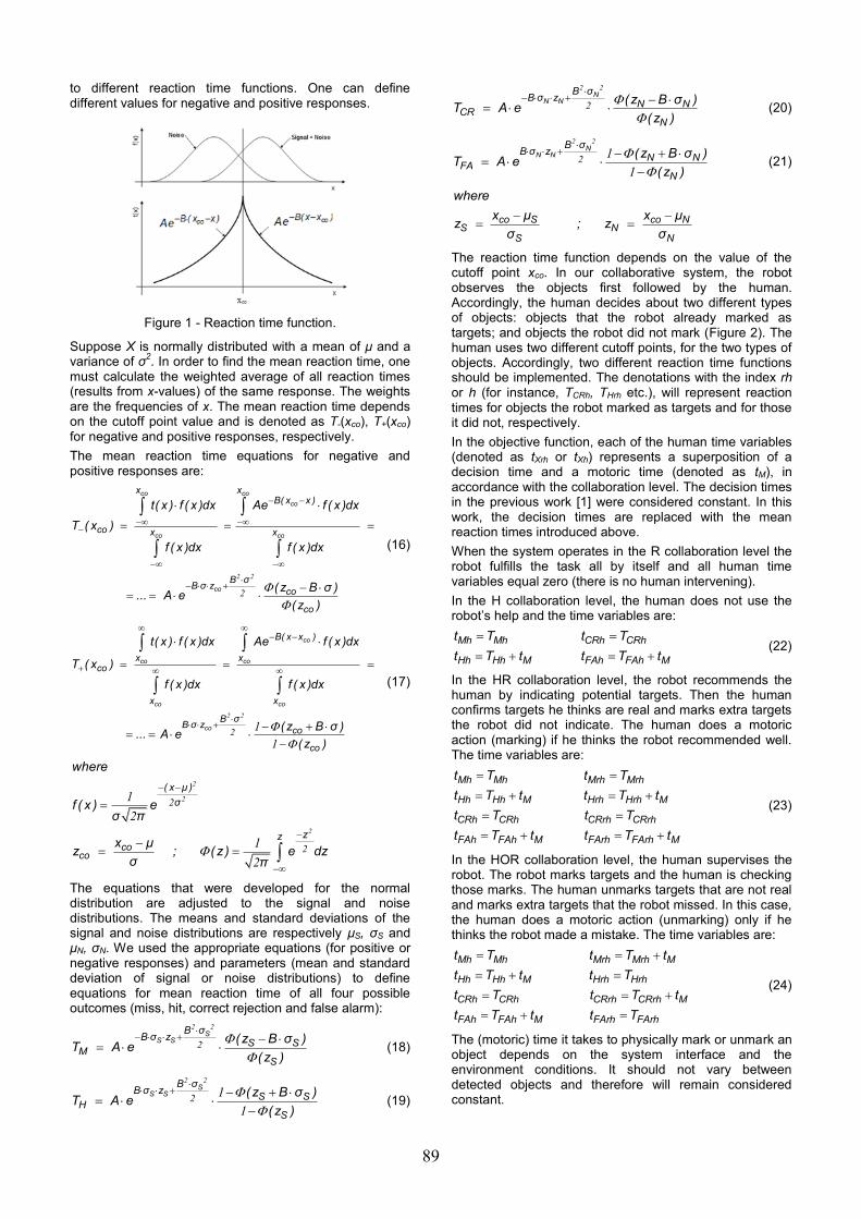
89
to different reaction time functions. One can define different values for negative and positive responses.
Figure 1 - Reaction time function.
Suppose X is normally distributed with a mean of μ and a variance of σ
2. In order to find the mean reaction time, one
must calculate the weighted average of all reaction times (results from x-values) of the same response. The weights are the frequencies of x. The mean reaction time depends on the cutoff point value and is denoted as T-(xco), T+(xco) for negative and positive responses, respectively.
The mean reaction time equations for negative and positive responses are:
2 2
2
co co
co
co co
co
x xB( x x )
co x x
B σB σ z
co
co
t( x ) f ( x )dx Ae f ( x )dx
T ( x )
f ( x )dx f ( x )dx
(z B σ )... A e
(z )
(16)
2 2
21
1
co
co co
co co
co
B( x x )
x xco
x x
B σB σ z
co
co
t( x ) f ( x )dx Ae f ( x )dx
T ( x )
f ( x )dx f ( x )dx
(z B σ )... A e
(z )
(17)
( x μ )
σ
zzco
co
where
f ( x ) eσ π
x μz ; ( z ) e dz
σ π
2
2
2
2
2
1
2
1
2
The equations that were developed for the normal distribution are adjusted to the signal and noise distributions. The means and standard deviations of the signal and noise distributions are respectively μS, σS and μN, σN. We used the appropriate equations (for positive or negative responses) and parameters (mean and standard deviation of signal or noise distributions) to define equations for mean reaction time of all four possible outcomes (miss, hit, correct rejection and false alarm):
2 2
2
SS S
B σB σ z
S SM
S
( z B σ )T A e
(z ) (18)
2 2
21
1
SS S
B σB σ z
S SH
S
( z B σ )T A e
(z ) (19)
2 2
2
NN N
B σB σ z
N NCR
N
( z B σ )T A e
(z ) (20)
2 2
21
1
NN N
B σB σ z
N NFA
N
( z B σ )T A e
(z ) (21)
co S co N
S NS N
where
x μ x μz ; z
σ σ
The reaction time function depends on the value of the cutoff point xco. In our collaborative system, the robot observes the objects first followed by the human. Accordingly, the human decides about two different types of objects: objects that the robot already marked as targets; and objects the robot did not mark (Figure 2). The human uses two different cutoff points, for the two types of objects. Accordingly, two different reaction time functions should be implemented. The denotations with the index rh or h (for instance, TCRh, THrh etc.), will represent reaction times for objects the robot marked as targets and for those it did not, respectively.
In the objective function, each of the human time variables (denoted as tXrh or tXh) represents a superposition of a decision time and a motoric time (denoted as tM), in accordance with the collaboration level. The decision times in the previous work [1] were considered constant. In this work, the decision times are replaced with the mean reaction times introduced above.
When the system operates in the R collaboration level the robot fulfills the task all by itself and all human time variables equal zero (there is no human intervening).
In the H collaboration level, the human does not use the robot‟s help and the time variables are:
Mh Mh CRh CRh
Hh Hh M FAh FAh M
t T t T
t T t t T t (22)
In the HR collaboration level, the robot recommends the human by indicating potential targets. Then the human confirms targets he thinks are real and marks extra targets the robot did not indicate. The human does a motoric action (marking) if he thinks the robot recommended well. The time variables are:
Mh Mh Mrh Mrh
Hh Hh M Hrh Hrh M
CRh CRh CRrh CRrh
FAh FAh M FArh FArh M
t T t T
t T t t T t
t T t T
t T t t T t
(23)
In the HOR collaboration level, the human supervises the robot. The robot marks targets and the human is checking those marks. The human unmarks targets that are not real and marks extra targets that the robot missed. In this case, the human does a motoric action (unmarking) only if he thinks the robot made a mistake. The time variables are:
Mh Mh Mrh Mrh M
Hh Hh M Hrh Hrh
CRh CRh CRrh CRrh M
FAh FAh M FArh FArh
t T t T t
t T t t T
t T t T t
t T t t T
(24)
The (motoric) time it takes to physically mark or unmark an object depends on the system interface and the environment conditions. It should not vary between detected objects and therefore will remain considered constant.

90
Figure 2 - Reaction times diagram.
3 NUMERICAL ANALYSIS
A numerical analysis of the model was conducted using MatLab 7.1 with optimal human and robot cutoff points. The optimal cutoff points were determined by finding the cutoff points that yielded the maximal objective function value. The objective function score was calculated for each possible combination of parameters and variables, for each collaboration level.
3.1 Model parameters
Task types and parameters
Analysis focused on three system types characterized by the gains and penalties for each outcome (VH,VM,VFA,VCR,
[10]). Table 1 details the values for each type of system.
Type I gives high priority for not doing errors of the first type, i.e., detecting a target when a target does not exist (false alarm).
Type II gives high priority for not doing errors of the second type, i.e., missing a target.
Type III systems do not prefer one type of error and therefore yield identical values for all four possible outcomes.
The time cost (VT) is the cost of one time unit of system operation. It includes the cost of the human operator and the robot since they are operating simultaneously. In order to analyze the influence of time cost regardless of the system type, it was set relatively to the gain for a hit (VT=VH∙VT2H). The ratio between the time cost and the gain for a hit, VT2H, was set to the values: -80, -40, -20 (hour
-1).
For example, when VH equals 5 points, VT obtained the
values: -400, -200, -100 points.
The operational cost (VC) is the cost of the action conducted when the system detects a target, either if it is a hit or a false alarm. This cost was set to 2 points.
Environmental parameters
The parameters N and PS determine the environmental
conditions. The objective function was calculated for 1,000 objects (N). The target probability (PS) represents the fraction of targets from all objects and received values between 0.1 and 0.9.
Human parameters
The decision time was calculated using the mean reaction time function introduced above. Parameter A, of the function, was set to 2, 5 or 10 seconds and parameter B was set to 0, 0.5, 1, 1.5 or 2. The human motoric time (tM) of executing an action was set to 2 seconds.
The sensitivity represents the ability of the observer to distinguish between real targets and the other objects. The human‟s sensitivity (d’h) was varied between 0.5 and 3.
Robot parameters
The sensitivity of the robot (d’r) was varied between 0.5 and 3. The robot decision time (tr) is negligible relatively to
the other times and was set to 0.01 seconds.
Table 1. Gains and penalties for different types of systems.
Type I Type II Type III
VH 5 50 10
VM -10 -10 -10
VFA -50 -5 -10
VCR 10 10 10
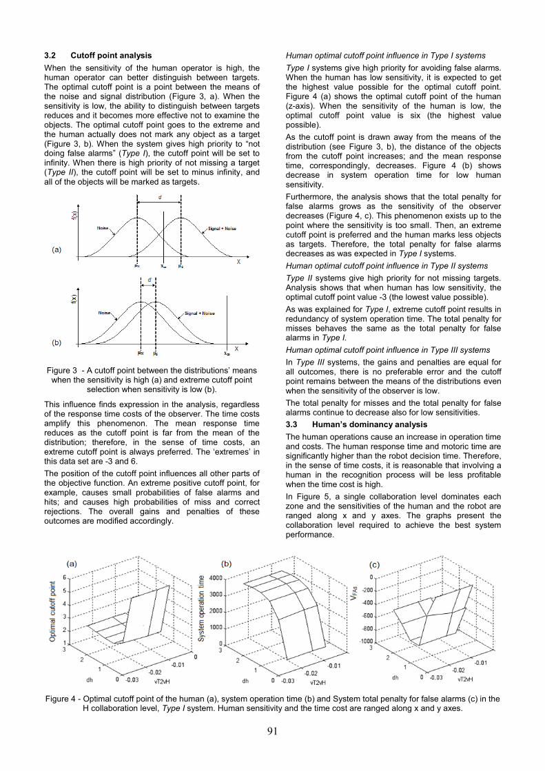
91
3.2 Cutoff point analysis
When the sensitivity of the human operator is high, the human operator can better distinguish between targets. The optimal cutoff point is a point between the means of the noise and signal distribution (Figure 3, a). When the sensitivity is low, the ability to distinguish between targets reduces and it becomes more effective not to examine the objects. The optimal cutoff point goes to the extreme and the human actually does not mark any object as a target (Figure 3, b). When the system gives high priority to “not doing false alarms” (Type I), the cutoff point will be set to infinity. When there is high priority of not missing a target (Type II), the cutoff point will be set to minus infinity, and
all of the objects will be marked as targets.
Figure 3 - A cutoff point between the distributions‟ means when the sensitivity is high (a) and extreme cutoff point
selection when sensitivity is low (b).
This influence finds expression in the analysis, regardless of the response time costs of the observer. The time costs amplify this phenomenon. The mean response time reduces as the cutoff point is far from the mean of the distribution; therefore, in the sense of time costs, an extreme cutoff point is always preferred. The „extremes‟ in this data set are -3 and 6.
The position of the cutoff point influences all other parts of the objective function. An extreme positive cutoff point, for example, causes small probabilities of false alarms and hits; and causes high probabilities of miss and correct rejections. The overall gains and penalties of these outcomes are modified accordingly.
Human optimal cutoff point influence in Type I systems
Type I systems give high priority for avoiding false alarms. When the human has low sensitivity, it is expected to get the highest value possible for the optimal cutoff point. Figure 4 (a) shows the optimal cutoff point of the human (z-axis). When the sensitivity of the human is low, the optimal cutoff point value is six (the highest value possible).
As the cutoff point is drawn away from the means of the distribution (see Figure 3, b), the distance of the objects from the cutoff point increases; and the mean response time, correspondingly, decreases. Figure 4 (b) shows decrease in system operation time for low human sensitivity.
Furthermore, the analysis shows that the total penalty for false alarms grows as the sensitivity of the observer decreases (Figure 4, c). This phenomenon exists up to the point where the sensitivity is too small. Then, an extreme cutoff point is preferred and the human marks less objects as targets. Therefore, the total penalty for false alarms decreases as was expected in Type I systems.
Human optimal cutoff point influence in Type II systems
Type II systems give high priority for not missing targets. Analysis shows that when human has low sensitivity, the optimal cutoff point value -3 (the lowest value possible).
As was explained for Type I, extreme cutoff point results in redundancy of system operation time. The total penalty for misses behaves the same as the total penalty for false alarms in Type I.
Human optimal cutoff point influence in Type III systems
In Type III systems, the gains and penalties are equal for all outcomes, there is no preferable error and the cutoff point remains between the means of the distributions even when the sensitivity of the observer is low.
The total penalty for misses and the total penalty for false alarms continue to decrease also for low sensitivities.
3.3 Human’s dominancy analysis
The human operations cause an increase in operation time and costs. The human response time and motoric time are significantly higher than the robot decision time. Therefore, in the sense of time costs, it is reasonable that involving a human in the recognition process will be less profitable when the time cost is high.
In Figure 5, a single collaboration level dominates each zone and the sensitivities of the human and the robot are ranged along x and y axes. The graphs present the collaboration level required to achieve the best system performance.
Figure 4 - Optimal cutoff point of the human (a), system operation time (b) and System total penalty for false alarms (c) in the H collaboration level, Type I system. Human sensitivity and the time cost are ranged along x and y axes.
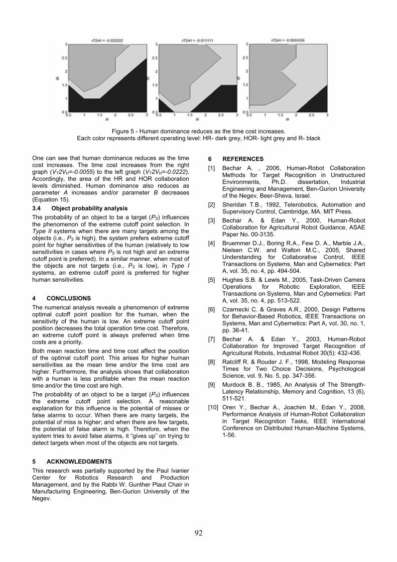
92
Figure 5 - Human dominance reduces as the time cost increases. Each color represents different operating level: HR- dark grey, HOR- light grey and R- black
One can see that human dominance reduces as the time cost increases. The time cost increases from the right graph (VT2VH=-0.0055) to the left graph (VT2VH=-0.0222). Accordingly, the area of the HR and HOR collaboration levels diminished. Human dominance also reduces as parameter A increases and/or parameter B decreases (Equation 15).
3.4 Object probability analysis
The probability of an object to be a target (PS) influences
the phenomenon of the extreme cutoff point selection. In Type II systems when there are many targets among the objects (i.e., PS is high), the system prefers extreme cutoff point for higher sensitivities of the human (relatively to low sensitivities in cases where PS is not high and an extreme cutoff point is preferred). In a similar manner, when most of the objects are not targets (i.e., PS is low), in Type I systems, an extreme cutoff point is preferred for higher human sensitivities.
4 CONCLUSIONS
The numerical analysis reveals a phenomenon of extreme optimal cutoff point position for the human, when the sensitivity of the human is low. An extreme cutoff point position decreases the total operation time cost. Therefore, an extreme cutoff point is always preferred when time costs are a priority.
Both mean reaction time and time cost affect the position of the optimal cutoff point. This arises for higher human sensitivities as the mean time and/or the time cost are higher. Furthermore, the analysis shows that collaboration with a human is less profitable when the mean reaction time and/or the time cost are high.
The probability of an object to be a target (PS) influences the extreme cutoff point selection. A reasonable explanation for this influence is the potential of misses or false alarms to occur. When there are many targets, the potential of miss is higher; and when there are few targets, the potential of false alarm is high. Therefore, when the system tries to avoid false alarms, it “gives up” on trying to detect targets when most of the objects are not targets.
5 ACKNOWLEDGMENTS
This research was partially supported by the Paul Ivanier Center for Robotics Research and Production Management, and by the Rabbi W. Gunther Plaut Chair in Manufacturing Engineering, Ben-Gurion University of the Negev.
6 REFERENCES
[1] Bechar A. , 2006, Human-Robot Collaboration Methods for Target Recognition in Unstructured Environments, Ph.D. dissertation, Industrial Engineering and Management, Ben-Gurion University of the Negev, Beer-Sheva, Israel.
[2] Sheridan T.B., 1992, Telerobotics, Automation and Supervisory Control, Cambridge, MA. MIT Press.
[3] Bechar A. & Edan Y., 2000, Human-Robot Collaboration for Agricultural Robot Guidance, ASAE Paper No. 00-3135.
[4] Bruemmer D.J., Boring R.A., Few D. A., Marble J.A., Nielsen C.W. and Walton M.C., 2005, Shared Understanding for Collaborative Control, IEEE Transactions on Systems, Man and Cybernetics: Part A, vol. 35, no. 4, pp. 494-504.
[5] Hughes S.B. & Lewis M., 2005, Task-Driven Camera Operations for Robotic Exploration, IEEE Transactions on Systems, Man and Cybernetics: Part A, vol. 35, no. 4, pp. 513-522.
[6] Czarnecki C. & Graves A.R., 2000, Design Patterns for Behavior-Based Robotics, IEEE Transactions on Systems, Man and Cybernetics: Part A, vol. 30, no. 1, pp. 36-41.
[7] Bechar A. & Edan Y., 2003, Human-Robot Collaboration for Improved Target Recognition of Agricultural Robots, Industrial Robot 30(5): 432-436.
[8] Ratcliff R. & Rouder J. F., 1998, Modeling Response Times for Two Choice Decisions, Psychological Science, vol. 9, No. 5, pp. 347-356.
[9] Murdock B. B., 1985, An Analysis of The Strength-Latency Relationship, Memory and Cognition, 13 (6), 511-521.
[10] Oren Y., Bechar A., Joachim M., Edan Y., 2008, Performance Analysis of Human-Robot Collaboration in Target Recognition Tasks, IEEE International Conference on Distributed Human-Machine Systems, 1-56.
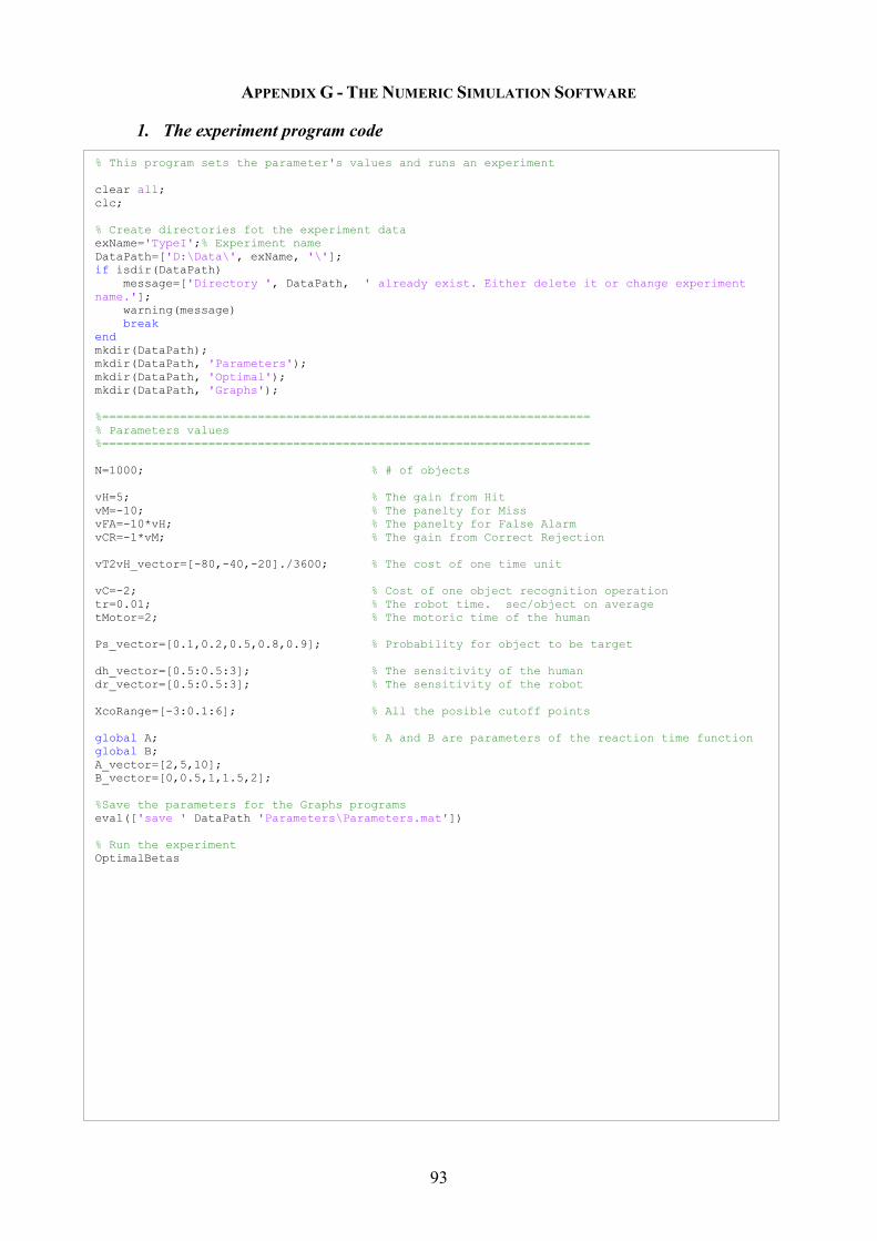
93
APPENDIX G - THE NUMERIC SIMULATION SOFTWARE
1. The experiment program code
% This program sets the parameter's values and runs an experiment
clear all;
clc;
% Create directories fot the experiment data
exName='TypeI';% Experiment name
DataPath=['D:\Data\', exName, '\'];
if isdir(DataPath)
message=['Directory ', DataPath, ' already exist. Either delete it or change experiment
name.'];
warning(message)
break
end
mkdir(DataPath);
mkdir(DataPath, 'Parameters');
mkdir(DataPath, 'Optimal');
mkdir(DataPath, 'Graphs');
%=====================================================================
% Parameters values
%=====================================================================
N=1000; % # of objects
vH=5; % The gain from Hit
vM=-10; % The panelty for Miss
vFA=-10*vH; % The panelty for False Alarm
vCR=-1*vM; % The gain from Correct Rejection
vT2vH_vector=[-80,-40,-20]./3600; % The cost of one time unit
vC=-2; % Cost of one object recognition operation
tr=0.01; % The robot time. sec/object on average
tMotor=2; % The motoric time of the human
Ps_vector=[0.1,0.2,0.5,0.8,0.9]; % Probability for object to be target
dh_vector=[0.5:0.5:3]; % The sensitivity of the human
dr_vector=[0.5:0.5:3]; % The sensitivity of the robot
XcoRange=[-3:0.1:6]; % All the posible cutoff points
global A; % A and B are parameters of the reaction time function
global B;
A_vector=[2,5,10];
B_vector=[0,0.5,1,1.5,2];
%Save the parameters for the Graphs programs
eval(['save ' DataPath 'Parameters\Parameters.mat'])
% Run the experiment
OptimalBetas
94
2. The data base creator code
% This program create a data set of all possible combination of the parameters. % Then, it extracts only the records of the optimal objective function value.
tic
% All possible cutoff points for the robot (r) and the human (h, rh), Based on their
sensitivities %-------------------------------------------------------------------------------------------
for i=1:sXco Zn_r(:,:,i)=XcoRange(i); Zn_h(:,i,:)=XcoRange(i); Zn_rh(i,:,:)=XcoRange(i); end
%===================================================================== % Loops 1 to 6 spread all combinations of parameters' values %=====================================================================
% Loop 1 : vT/vH aspect ratio for ivT2vH = 1:length(vT2vH_vector) vT=vH.*vT2vH_vector(ivT2vH);
% Loop 2 : B parameter of the mean time function for iB=1:length(B_vector) B=B_vector(iB);
% Loop 3: A parameter of the mean time function for iA=1:length(A_vector) A=A_vector(iA);
% Loop 4 : Probability for object to be target for iPs=1:length(Ps_vector) Ps=Ps_vector(iPs);
% Loop 5 : The range of d' for the human operator sensitivity for idh=1:length(dh_vector) dh=dh_vector(idh);
% Loop 6 : The range of d' for the robot sensitivity for idr=1:length(dr_vector) dr=dr_vector(idr);
%============================================================================================ % START - For each combination of parameters - create data set of all possible cutoff points %============================================================================================ % All possible cutoff points for the robot(r) and the human(h,rh). Based on their sensitivities %-------------------------------------------------------------------------------------------
Zs_r=Zn_r-dr; % Robot's cutoff point for a signal Zs_h=Zn_h-dh; % Human's cutoff point for a signal Zs_rh=Zn_rh-dh; % Human's cutoff point for a signal, when collaborate with the robot
% The probabilities for the robot (r) and the human (h, rh). Based on the cutoff points %-------------------------------------------------------------------------------------------
pH_r=1-normcdf(Zs_r); % Robot's probability for a hit pFA_r=1-normcdf(Zn_r); % Robot's probability for a false alarm pH_h=1-normcdf(Zs_h); % Human's probability for a hit pFA_h=1-normcdf(Zn_h); % Human's probability for a false alarm pH_rh=1-normcdf(Zs_rh); % Human's probability for a hit, when collaborate with the robot pFA_rh=1-normcdf(Zn_rh); % Human's probability for a FA, when collaborate with the robot
% The mean response time of the human for objects the robot did not mark %-------------------------------------------------------------------------------------------
tH_h=meanTime(Zs_h,'p'); tM_h=meanTime(Zs_h,'n'); tFA_h=meanTime(Zn_h,'p'); tCR_h=meanTime(Zn_h,'n');
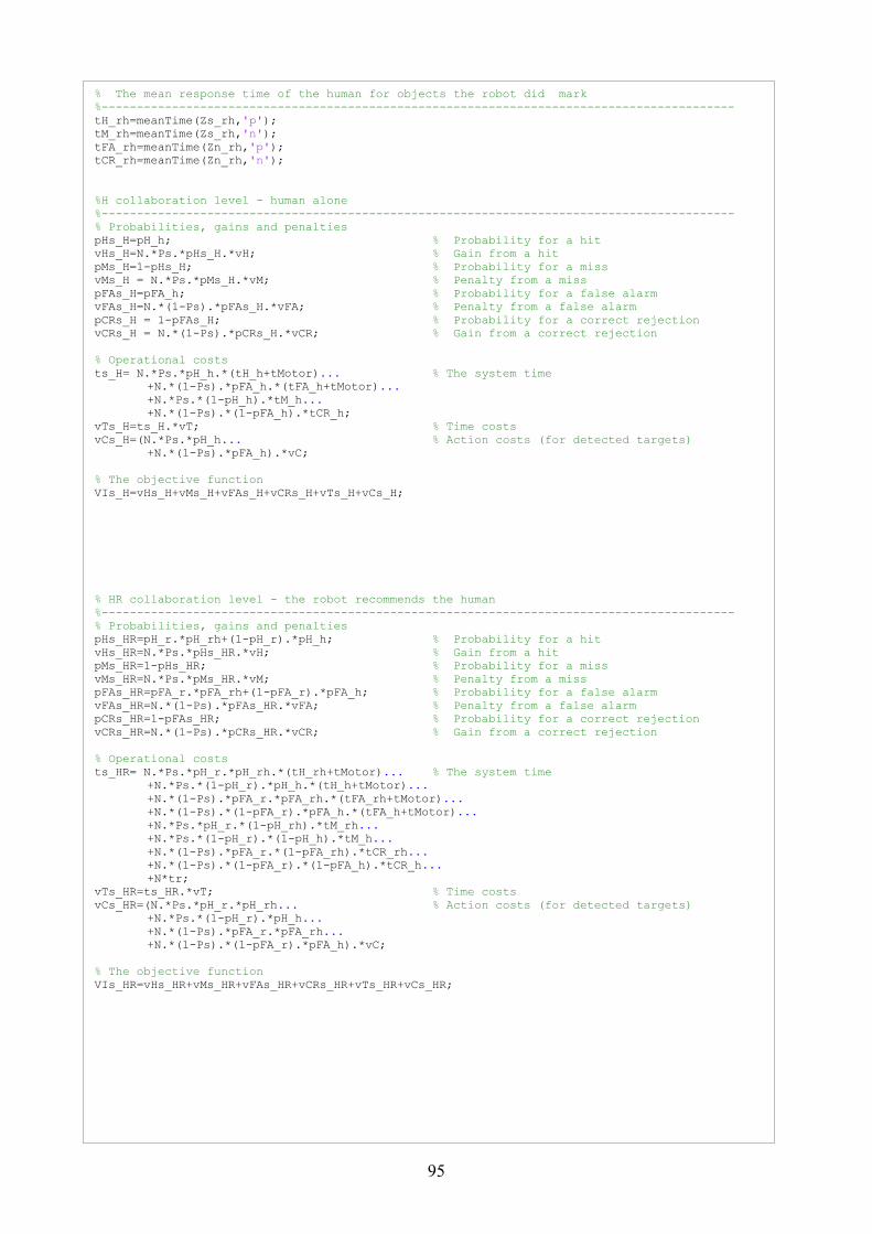
95
% The mean response time of the human for objects the robot did mark
%------------------------------------------------------------------------------------------
tH_rh=meanTime(Zs_rh,'p');
tM_rh=meanTime(Zs_rh,'n');
tFA_rh=meanTime(Zn_rh,'p');
tCR_rh=meanTime(Zn_rh,'n');
%H collaboration level - human alone
%------------------------------------------------------------------------------------------
% Probabilities, gains and penalties
pHs_H=pH_h; % Probability for a hit
vHs_H=N.*Ps.*pHs_H.*vH; % Gain from a hit
pMs_H=1-pHs_H; % Probability for a miss
vMs_H = N.*Ps.*pMs_H.*vM; % Penalty from a miss
pFAs_H=pFA_h; % Probability for a false alarm
vFAs_H=N.*(1-Ps).*pFAs_H.*vFA; % Penalty from a false alarm
pCRs_H = 1-pFAs_H; % Probability for a correct rejection
vCRs_H = N.*(1-Ps).*pCRs_H.*vCR; % Gain from a correct rejection
% Operational costs
ts_H= N.*Ps.*pH_h.*(tH_h+tMotor)... % The system time
+N.*(1-Ps).*pFA_h.*(tFA_h+tMotor)...
+N.*Ps.*(1-pH_h).*tM_h...
+N.*(1-Ps).*(1-pFA_h).*tCR_h;
vTs_H=ts_H.*vT; % Time costs
vCs_H=(N.*Ps.*pH_h... % Action costs (for detected targets)
+N.*(1-Ps).*pFA_h).*vC;
% The objective function
VIs_H=vHs_H+vMs_H+vFAs_H+vCRs_H+vTs_H+vCs_H;
% HR collaboration level - the robot recommends the human
%------------------------------------------------------------------------------------------
% Probabilities, gains and penalties
pHs_HR=pH_r.*pH_rh+(1-pH_r).*pH_h; % Probability for a hit
vHs_HR=N.*Ps.*pHs_HR.*vH; % Gain from a hit
pMs_HR=1-pHs_HR; % Probability for a miss
vMs_HR=N.*Ps.*pMs_HR.*vM; % Penalty from a miss
pFAs_HR=pFA_r.*pFA_rh+(1-pFA_r).*pFA_h; % Probability for a false alarm
vFAs_HR=N.*(1-Ps).*pFAs_HR.*vFA; % Penalty from a false alarm
pCRs_HR=1-pFAs_HR; % Probability for a correct rejection
vCRs_HR=N.*(1-Ps).*pCRs_HR.*vCR; % Gain from a correct rejection
% Operational costs
ts_HR= N.*Ps.*pH_r.*pH_rh.*(tH_rh+tMotor)... % The system time
+N.*Ps.*(1-pH_r).*pH_h.*(tH_h+tMotor)...
+N.*(1-Ps).*pFA_r.*pFA_rh.*(tFA_rh+tMotor)...
+N.*(1-Ps).*(1-pFA_r).*pFA_h.*(tFA_h+tMotor)...
+N.*Ps.*pH_r.*(1-pH_rh).*tM_rh...
+N.*Ps.*(1-pH_r).*(1-pH_h).*tM_h...
+N.*(1-Ps).*pFA_r.*(1-pFA_rh).*tCR_rh...
+N.*(1-Ps).*(1-pFA_r).*(1-pFA_h).*tCR_h...
+N*tr;
vTs_HR=ts_HR.*vT; % Time costs
vCs_HR=(N.*Ps.*pH_r.*pH_rh... % Action costs (for detected targets)
+N.*Ps.*(1-pH_r).*pH_h...
+N.*(1-Ps).*pFA_r.*pFA_rh...
+N.*(1-Ps).*(1-pFA_r).*pFA_h).*vC;
% The objective function
VIs_HR=vHs_HR+vMs_HR+vFAs_HR+vCRs_HR+vTs_HR+vCs_HR;
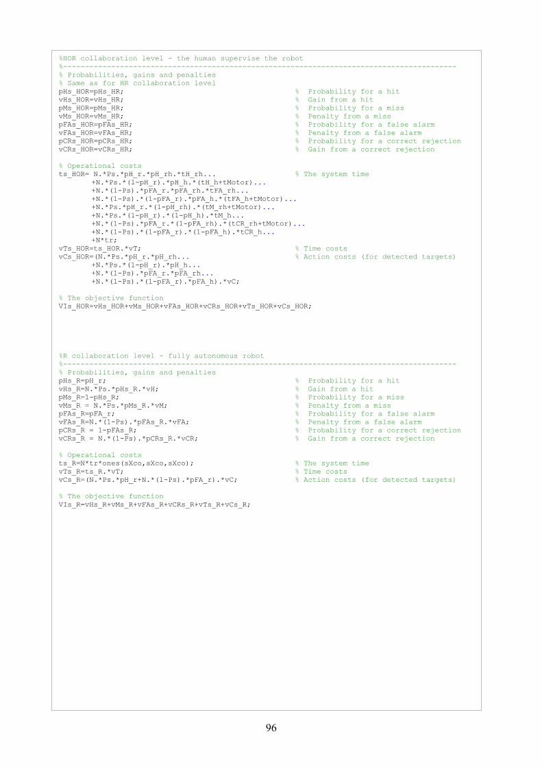
96
%HOR collaboration level - the human supervise the robot
%------------------------------------------------------------------------------------------
% Probabilities, gains and penalties
% Same as for HR collaboration level
pHs_HOR=pHs_HR; % Probability for a hit
vHs_HOR=vHs_HR; % Gain from a hit
pMs_HOR=pMs_HR; % Probability for a miss
vMs_HOR=vMs_HR; % Penalty from a miss
pFAs_HOR=pFAs_HR; % Probability for a false alarm
vFAs_HOR=vFAs_HR; % Penalty from a false alarm
pCRs_HOR=pCRs_HR; % Probability for a correct rejection
vCRs_HOR=vCRs_HR; % Gain from a correct rejection
% Operational costs
ts_HOR= N.*Ps.*pH_r.*pH_rh.*tH_rh... % The system time
+N.*Ps.*(1-pH_r).*pH_h.*(tH_h+tMotor)...
+N.*(1-Ps).*pFA_r.*pFA_rh.*tFA_rh...
+N.*(1-Ps).*(1-pFA_r).*pFA_h.*(tFA_h+tMotor)...
+N.*Ps.*pH_r.*(1-pH_rh).*(tM_rh+tMotor)...
+N.*Ps.*(1-pH_r).*(1-pH_h).*tM_h...
+N.*(1-Ps).*pFA_r.*(1-pFA_rh).*(tCR_rh+tMotor)...
+N.*(1-Ps).*(1-pFA_r).*(1-pFA_h).*tCR_h...
+N*tr;
vTs_HOR=ts_HOR.*vT; % Time costs
vCs_HOR=(N.*Ps.*pH_r.*pH_rh... % Action costs (for detected targets)
+N.*Ps.*(1-pH_r).*pH_h...
+N.*(1-Ps).*pFA_r.*pFA_rh...
+N.*(1-Ps).*(1-pFA_r).*pFA_h).*vC;
% The objective function
VIs_HOR=vHs_HOR+vMs_HOR+vFAs_HOR+vCRs_HOR+vTs_HOR+vCs_HOR;
%R collaboration level - fully autonomous robot
%------------------------------------------------------------------------------------------
% Probabilities, gains and penalties
pHs_R=pH_r; % Probability for a hit
vHs_R=N.*Ps.*pHs_R.*vH; % Gain from a hit
pMs_R=1-pHs_R; % Probability for a miss
vMs_R = N.*Ps.*pMs_R.*vM; % Penalty from a miss
pFAs_R=pFA_r; % Probability for a false alarm
vFAs_R=N.*(1-Ps).*pFAs_R.*vFA; % Penalty from a false alarm
pCRs_R = 1-pFAs_R; % Probability for a correct rejection
vCRs_R = N.*(1-Ps).*pCRs_R.*vCR; % Gain from a correct rejection
% Operational costs
ts_R=N*tr*ones(sXco,sXco,sXco); % The system time
vTs_R=ts_R.*vT; % Time costs
vCs_R=(N.*Ps.*pH_r+N.*(1-Ps).*pFA_r).*vC; % Action costs (for detected targets)
% The objective function
VIs_R=vHs_R+vMs_R+vFAs_R+vCRs_R+vTs_R+vCs_R;
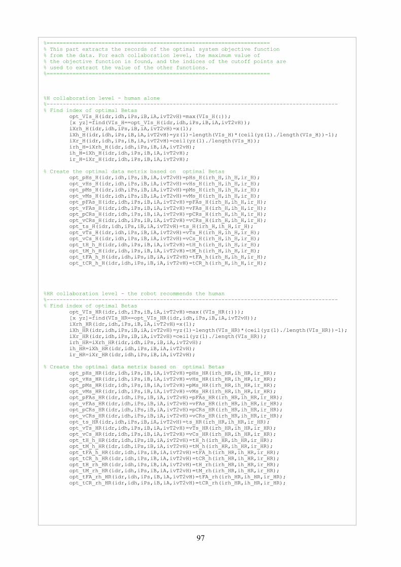
97
%=====================================================================
% This part extracts the records of the optimal system objective function
% from the data. For each collaboration level, the maximum value of
% the objective function is found, and the indices of the cutoff points are
% used to extract the value of the other functions.
%=====================================================================
%H collaboration level - human alone
%------------------------------------------------------------------------------------------
% Find index of optimal Betas
opt_VIs_H(idr,idh,iPs,iB,iA,ivT2vH)=max(VIs_H(:));
[x yz]=find(VIs_H==opt_VIs_H(idr,idh,iPs,iB,iA,ivT2vH));
iXrh_H(idr,idh,iPs,iB,iA,ivT2vH)=x(1);
iXh_H(idr,idh,iPs,iB,iA,ivT2vH)=yz(1)-length(VIs_H)*(ceil(yz(1)./length(VIs_H))-1);
iXr_H(idr,idh,iPs,iB,iA,ivT2vH)=ceil(yz(1)./length(VIs_H));
irh_H=iXrh_H(idr,idh,iPs,iB,iA,ivT2vH);
ih_H=iXh_H(idr,idh,iPs,iB,iA,ivT2vH);
ir_H=iXr_H(idr,idh,iPs,iB,iA,ivT2vH);
% Create the optimal data metrix based on optimal Betas
opt_pHs_H(idr,idh,iPs,iB,iA,ivT2vH)=pHs_H(irh_H,ih_H,ir_H);
opt_vHs_H(idr,idh,iPs,iB,iA,ivT2vH)=vHs_H(irh_H,ih_H,ir_H);
opt_pMs_H(idr,idh,iPs,iB,iA,ivT2vH)=pMs_H(irh_H,ih_H,ir_H);
opt_vMs_H(idr,idh,iPs,iB,iA,ivT2vH)=vMs_H(irh_H,ih_H,ir_H);
opt_pFAs_H(idr,idh,iPs,iB,iA,ivT2vH)=pFAs_H(irh_H,ih_H,ir_H);
opt_vFAs_H(idr,idh,iPs,iB,iA,ivT2vH)=vFAs_H(irh_H,ih_H,ir_H);
opt_pCRs_H(idr,idh,iPs,iB,iA,ivT2vH)=pCRs_H(irh_H,ih_H,ir_H);
opt_vCRs_H(idr,idh,iPs,iB,iA,ivT2vH)=vCRs_H(irh_H,ih_H,ir_H);
opt_ts_H(idr,idh,iPs,iB,iA,ivT2vH)=ts_H(irh_H,ih_H,ir_H);
opt_vTs_H(idr,idh,iPs,iB,iA,ivT2vH)=vTs_H(irh_H,ih_H,ir_H);
opt_vCs_H(idr,idh,iPs,iB,iA,ivT2vH)=vCs_H(irh_H,ih_H,ir_H);
opt_tH_h_H(idr,idh,iPs,iB,iA,ivT2vH)=tH_h(irh_H,ih_H,ir_H);
opt_tM_h_H(idr,idh,iPs,iB,iA,ivT2vH)=tM_h(irh_H,ih_H,ir_H);
opt_tFA_h_H(idr,idh,iPs,iB,iA,ivT2vH)=tFA_h(irh_H,ih_H,ir_H);
opt_tCR_h_H(idr,idh,iPs,iB,iA,ivT2vH)=tCR_h(irh_H,ih_H,ir_H);
%HR collaboration level - the robot recommends the human
%------------------------------------------------------------------------------------------
% Find index of optimal Betas
opt_VIs_HR(idr,idh,iPs,iB,iA,ivT2vH)=max((VIs_HR(:)));
[x yz]=find(VIs_HR==opt_VIs_HR(idr,idh,iPs,iB,iA,ivT2vH));
iXrh_HR(idr,idh,iPs,iB,iA,ivT2vH)=x(1);
iXh_HR(idr,idh,iPs,iB,iA,ivT2vH)=yz(1)-length(VIs_HR)*(ceil(yz(1)./length(VIs_HR))-1);
iXr_HR(idr,idh,iPs,iB,iA,ivT2vH)=ceil(yz(1)./length(VIs_HR));
irh_HR=iXrh_HR(idr,idh,iPs,iB,iA,ivT2vH);
ih_HR=iXh_HR(idr,idh,iPs,iB,iA,ivT2vH);
ir_HR=iXr_HR(idr,idh,iPs,iB,iA,ivT2vH);
% Create the optimal data metrix based on optimal Betas
opt_pHs_HR(idr,idh,iPs,iB,iA,ivT2vH)=pHs_HR(irh_HR,ih_HR,ir_HR);
opt_vHs_HR(idr,idh,iPs,iB,iA,ivT2vH)=vHs_HR(irh_HR,ih_HR,ir_HR);
opt_pMs_HR(idr,idh,iPs,iB,iA,ivT2vH)=pMs_HR(irh_HR,ih_HR,ir_HR);
opt_vMs_HR(idr,idh,iPs,iB,iA,ivT2vH)=vMs_HR(irh_HR,ih_HR,ir_HR);
opt_pFAs_HR(idr,idh,iPs,iB,iA,ivT2vH)=pFAs_HR(irh_HR,ih_HR,ir_HR);
opt_vFAs_HR(idr,idh,iPs,iB,iA,ivT2vH)=vFAs_HR(irh_HR,ih_HR,ir_HR);
opt_pCRs_HR(idr,idh,iPs,iB,iA,ivT2vH)=pCRs_HR(irh_HR,ih_HR,ir_HR);
opt_vCRs_HR(idr,idh,iPs,iB,iA,ivT2vH)=vCRs_HR(irh_HR,ih_HR,ir_HR);
opt_ts_HR(idr,idh,iPs,iB,iA,ivT2vH)=ts_HR(irh_HR,ih_HR,ir_HR);
opt_vTs_HR(idr,idh,iPs,iB,iA,ivT2vH)=vTs_HR(irh_HR,ih_HR,ir_HR);
opt_vCs_HR(idr,idh,iPs,iB,iA,ivT2vH)=vCs_HR(irh_HR,ih_HR,ir_HR);
opt_tH_h_HR(idr,idh,iPs,iB,iA,ivT2vH)=tH_h(irh_HR,ih_HR,ir_HR);
opt_tM_h_HR(idr,idh,iPs,iB,iA,ivT2vH)=tM_h(irh_HR,ih_HR,ir_HR);
opt_tFA_h_HR(idr,idh,iPs,iB,iA,ivT2vH)=tFA_h(irh_HR,ih_HR,ir_HR);
opt_tCR_h_HR(idr,idh,iPs,iB,iA,ivT2vH)=tCR_h(irh_HR,ih_HR,ir_HR);
opt_tH_rh_HR(idr,idh,iPs,iB,iA,ivT2vH)=tH_rh(irh_HR,ih_HR,ir_HR);
opt_tM_rh_HR(idr,idh,iPs,iB,iA,ivT2vH)=tM_rh(irh_HR,ih_HR,ir_HR);
opt_tFA_rh_HR(idr,idh,iPs,iB,iA,ivT2vH)=tFA_rh(irh_HR,ih_HR,ir_HR);
opt_tCR_rh_HR(idr,idh,iPs,iB,iA,ivT2vH)=tCR_rh(irh_HR,ih_HR,ir_HR);
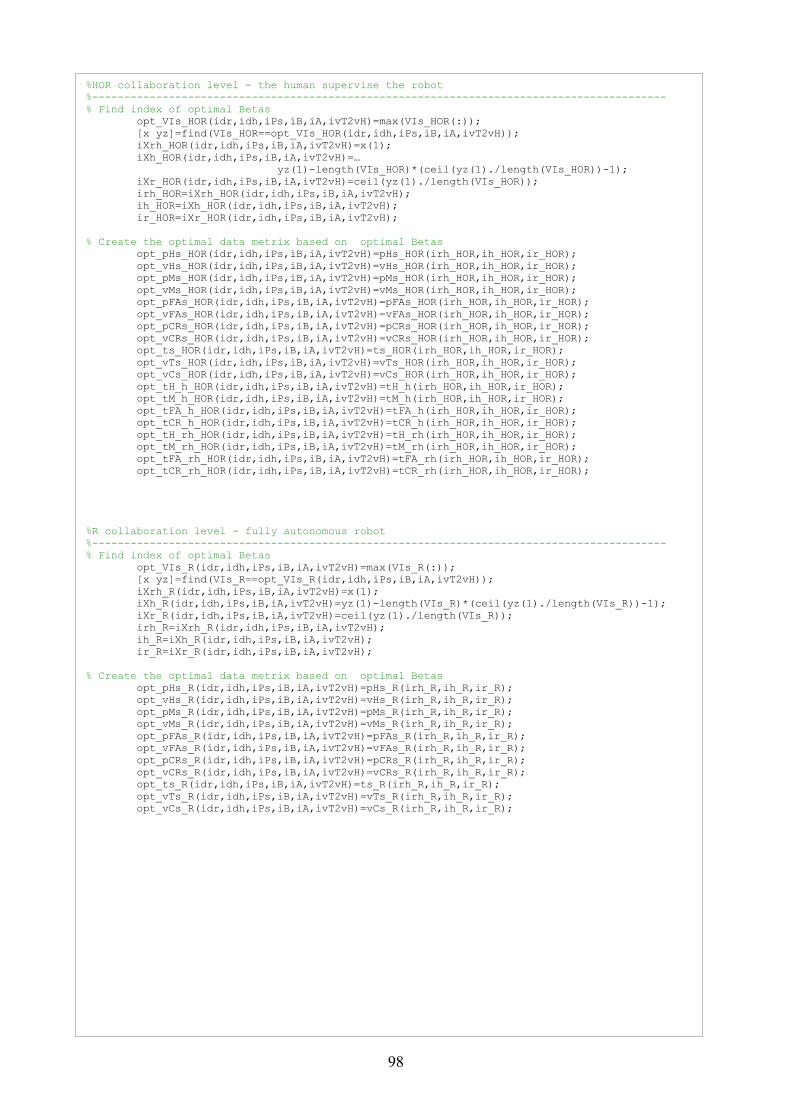
98
%HOR collaboration level - the human supervise the robot
%------------------------------------------------------------------------------------------
% Find index of optimal Betas
opt_VIs_HOR(idr,idh,iPs,iB,iA,ivT2vH)=max(VIs_HOR(:));
[x yz]=find(VIs_HOR==opt_VIs_HOR(idr,idh,iPs,iB,iA,ivT2vH));
iXrh_HOR(idr,idh,iPs,iB,iA,ivT2vH)=x(1);
iXh_HOR(idr,idh,iPs,iB,iA,ivT2vH)=…
yz(1)-length(VIs_HOR)*(ceil(yz(1)./length(VIs_HOR))-1);
iXr_HOR(idr,idh,iPs,iB,iA,ivT2vH)=ceil(yz(1)./length(VIs_HOR));
irh_HOR=iXrh_HOR(idr,idh,iPs,iB,iA,ivT2vH);
ih_HOR=iXh_HOR(idr,idh,iPs,iB,iA,ivT2vH);
ir_HOR=iXr_HOR(idr,idh,iPs,iB,iA,ivT2vH);
% Create the optimal data metrix based on optimal Betas
opt_pHs_HOR(idr,idh,iPs,iB,iA,ivT2vH)=pHs_HOR(irh_HOR,ih_HOR,ir_HOR);
opt_vHs_HOR(idr,idh,iPs,iB,iA,ivT2vH)=vHs_HOR(irh_HOR,ih_HOR,ir_HOR);
opt_pMs_HOR(idr,idh,iPs,iB,iA,ivT2vH)=pMs_HOR(irh_HOR,ih_HOR,ir_HOR);
opt_vMs_HOR(idr,idh,iPs,iB,iA,ivT2vH)=vMs_HOR(irh_HOR,ih_HOR,ir_HOR);
opt_pFAs_HOR(idr,idh,iPs,iB,iA,ivT2vH)=pFAs_HOR(irh_HOR,ih_HOR,ir_HOR);
opt_vFAs_HOR(idr,idh,iPs,iB,iA,ivT2vH)=vFAs_HOR(irh_HOR,ih_HOR,ir_HOR);
opt_pCRs_HOR(idr,idh,iPs,iB,iA,ivT2vH)=pCRs_HOR(irh_HOR,ih_HOR,ir_HOR);
opt_vCRs_HOR(idr,idh,iPs,iB,iA,ivT2vH)=vCRs_HOR(irh_HOR,ih_HOR,ir_HOR);
opt_ts_HOR(idr,idh,iPs,iB,iA,ivT2vH)=ts_HOR(irh_HOR,ih_HOR,ir_HOR);
opt_vTs_HOR(idr,idh,iPs,iB,iA,ivT2vH)=vTs_HOR(irh_HOR,ih_HOR,ir_HOR);
opt_vCs_HOR(idr,idh,iPs,iB,iA,ivT2vH)=vCs_HOR(irh_HOR,ih_HOR,ir_HOR);
opt_tH_h_HOR(idr,idh,iPs,iB,iA,ivT2vH)=tH_h(irh_HOR,ih_HOR,ir_HOR);
opt_tM_h_HOR(idr,idh,iPs,iB,iA,ivT2vH)=tM_h(irh_HOR,ih_HOR,ir_HOR);
opt_tFA_h_HOR(idr,idh,iPs,iB,iA,ivT2vH)=tFA_h(irh_HOR,ih_HOR,ir_HOR);
opt_tCR_h_HOR(idr,idh,iPs,iB,iA,ivT2vH)=tCR_h(irh_HOR,ih_HOR,ir_HOR);
opt_tH_rh_HOR(idr,idh,iPs,iB,iA,ivT2vH)=tH_rh(irh_HOR,ih_HOR,ir_HOR);
opt_tM_rh_HOR(idr,idh,iPs,iB,iA,ivT2vH)=tM_rh(irh_HOR,ih_HOR,ir_HOR);
opt_tFA_rh_HOR(idr,idh,iPs,iB,iA,ivT2vH)=tFA_rh(irh_HOR,ih_HOR,ir_HOR);
opt_tCR_rh_HOR(idr,idh,iPs,iB,iA,ivT2vH)=tCR_rh(irh_HOR,ih_HOR,ir_HOR);
%R collaboration level - fully autonomous robot
%------------------------------------------------------------------------------------------
% Find index of optimal Betas
opt_VIs_R(idr,idh,iPs,iB,iA,ivT2vH)=max(VIs_R(:));
[x yz]=find(VIs_R==opt_VIs_R(idr,idh,iPs,iB,iA,ivT2vH));
iXrh_R(idr,idh,iPs,iB,iA,ivT2vH)=x(1);
iXh_R(idr,idh,iPs,iB,iA,ivT2vH)=yz(1)-length(VIs_R)*(ceil(yz(1)./length(VIs_R))-1);
iXr_R(idr,idh,iPs,iB,iA,ivT2vH)=ceil(yz(1)./length(VIs_R));
irh_R=iXrh_R(idr,idh,iPs,iB,iA,ivT2vH);
ih_R=iXh_R(idr,idh,iPs,iB,iA,ivT2vH);
ir_R=iXr_R(idr,idh,iPs,iB,iA,ivT2vH);
% Create the optimal data metrix based on optimal Betas
opt_pHs_R(idr,idh,iPs,iB,iA,ivT2vH)=pHs_R(irh_R,ih_R,ir_R);
opt_vHs_R(idr,idh,iPs,iB,iA,ivT2vH)=vHs_R(irh_R,ih_R,ir_R);
opt_pMs_R(idr,idh,iPs,iB,iA,ivT2vH)=pMs_R(irh_R,ih_R,ir_R);
opt_vMs_R(idr,idh,iPs,iB,iA,ivT2vH)=vMs_R(irh_R,ih_R,ir_R);
opt_pFAs_R(idr,idh,iPs,iB,iA,ivT2vH)=pFAs_R(irh_R,ih_R,ir_R);
opt_vFAs_R(idr,idh,iPs,iB,iA,ivT2vH)=vFAs_R(irh_R,ih_R,ir_R);
opt_pCRs_R(idr,idh,iPs,iB,iA,ivT2vH)=pCRs_R(irh_R,ih_R,ir_R);
opt_vCRs_R(idr,idh,iPs,iB,iA,ivT2vH)=vCRs_R(irh_R,ih_R,ir_R);
opt_ts_R(idr,idh,iPs,iB,iA,ivT2vH)=ts_R(irh_R,ih_R,ir_R);
opt_vTs_R(idr,idh,iPs,iB,iA,ivT2vH)=vTs_R(irh_R,ih_R,ir_R);
opt_vCs_R(idr,idh,iPs,iB,iA,ivT2vH)=vCs_R(irh_R,ih_R,ir_R);
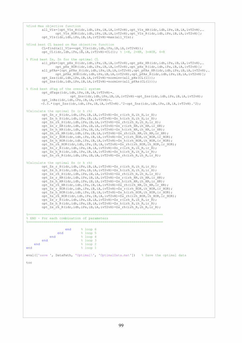
99
%find Max objective function
all_VIs=[opt_VIs_H(idr,idh,iPs,iB,iA,ivT2vH),opt_VIs_HR(idr,idh,iPs,iB,iA,ivT2vH),…
opt_VIs_HOR(idr,idh,iPs,iB,iA,ivT2vH),opt_VIs_R(idr,idh,iPs,iB,iA,ivT2vH)];
opt_VIs(idr,idh,iPs,iB,iA,ivT2vH)=max(all_VIs);
%find best CL based on Max objective function
CL=find(all_VIs==opt_VIs(idr,idh,iPs,iB,iA,ivT2vH));
opt_CL(idr,idh,iPs,iB,iA,ivT2vH)=CL(1); % 1=H, 2=HR, 3=HOR, 4=R
% Find best Zs, Zn for the optimal CL
all_pHs=[opt_pHs_H(idr,idh,iPs,iB,iA,ivT2vH),opt_pHs_HR(idr,idh,iPs,iB,iA,ivT2vH),…
opt_pHs_HOR(idr,idh,iPs,iB,iA,ivT2vH),opt_pHs_R(idr,idh,iPs,iB,iA,ivT2vH)];
all_pFAs=[opt_pFAs_H(idr,idh,iPs,iB,iA,ivT2vH),opt_pFAs_HR(idr,idh,iPs,iB,iA,ivT2vH),…
opt_pFAs_HOR(idr,idh,iPs,iB,iA,ivT2vH),opt_pFAs_R(idr,idh,iPs,iB,iA,ivT2vH)];
opt_Zss(idr,idh,iPs,iB,iA,ivT2vH)=norminv(all_pHs(CL(1)));
opt_Zns(idr,idh,iPs,iB,iA,ivT2vH)=norminv(all_pFAs(CL(1)));
% find best dTag of the overall system
opt_dTags(idr,idh,iPs,iB,iA,ivT2vH)=…
opt_Zns(idr,idh,iPs,iB,iA,ivT2vH)-opt_Zss(idr,idh,iPs,iB,iA,ivT2vH);
opt_lnBs(idr,idh,iPs,iB,iA,ivT2vH)=…
-0.5.*(opt_Zss(idr,idh,iPs,iB,iA,ivT2vH).^2-opt_Zns(idr,idh,iPs,iB,iA,ivT2vH).^2);
%Calculate the optimal Zn (r h rh)
opt_Zn_r_H(idr,idh,iPs,iB,iA,ivT2vH)=Zn_r(irh_H,ih_H,ir_H);
opt_Zn_h_H(idr,idh,iPs,iB,iA,ivT2vH)=Zn_h(irh_H,ih_H,ir_H);
opt_Zn_rh_H(idr,idh,iPs,iB,iA,ivT2vH)=Zn_rh(irh_H,ih_H,ir_H);
opt_Zn_r_HR(idr,idh,iPs,iB,iA,ivT2vH)=Zn_r(irh_HR,ih_HR,ir_HR);
opt_Zn_h_HR(idr,idh,iPs,iB,iA,ivT2vH)=Zn_h(irh_HR,ih_HR,ir_HR);
opt_Zn_rh_HR(idr,idh,iPs,iB,iA,ivT2vH)=Zn_rh(irh_HR,ih_HR,ir_HR);
opt_Zn_r_HOR(idr,idh,iPs,iB,iA,ivT2vH)=Zn_r(irh_HOR,ih_HOR,ir_HOR);
opt_Zn_h_HOR(idr,idh,iPs,iB,iA,ivT2vH)=Zn_h(irh_HOR,ih_HOR,ir_HOR);
opt_Zn_rh_HOR(idr,idh,iPs,iB,iA,ivT2vH)=Zn_rh(irh_HOR,ih_HOR,ir_HOR);
opt_Zn_r_R(idr,idh,iPs,iB,iA,ivT2vH)=Zn_r(irh_R,ih_R,ir_R);
opt_Zn_h_R(idr,idh,iPs,iB,iA,ivT2vH)=Zn_h(irh_R,ih_R,ir_R);
opt_Zn_rh_R(idr,idh,iPs,iB,iA,ivT2vH)=Zn_rh(irh_R,ih_R,ir_R);
%Calculate the optimal Zs (r h rh)
opt_Zs_r_H(idr,idh,iPs,iB,iA,ivT2vH)=Zs_r(irh_H,ih_H,ir_H);
opt_Zs_h_H(idr,idh,iPs,iB,iA,ivT2vH)=Zs_h(irh_H,ih_H,ir_H);
opt_Zs_rh_H(idr,idh,iPs,iB,iA,ivT2vH)=Zs_rh(irh_H,ih_H,ir_H);
opt_Zs_r_HR(idr,idh,iPs,iB,iA,ivT2vH)=Zs_r(irh_HR,ih_HR,ir_HR);
opt_Zs_h_HR(idr,idh,iPs,iB,iA,ivT2vH)=Zs_h(irh_HR,ih_HR,ir_HR);
opt_Zs_rh_HR(idr,idh,iPs,iB,iA,ivT2vH)=Zs_rh(irh_HR,ih_HR,ir_HR);
opt_Zs_r_HOR(idr,idh,iPs,iB,iA,ivT2vH)=Zs_r(irh_HOR,ih_HOR,ir_HOR);
opt_Zs_h_HOR(idr,idh,iPs,iB,iA,ivT2vH)=Zs_h(irh_HOR,ih_HOR,ir_HOR);
opt_Zs_rh_HOR(idr,idh,iPs,iB,iA,ivT2vH)=Zs_rh(irh_HOR,ih_HOR,ir_HOR);
opt_Zs_r_R(idr,idh,iPs,iB,iA,ivT2vH)=Zs_r(irh_R,ih_R,ir_R);
opt_Zs_h_R(idr,idh,iPs,iB,iA,ivT2vH)=Zs_h(irh_R,ih_R,ir_R);
opt_Zs_rh_R(idr,idh,iPs,iB,iA,ivT2vH)=Zs_rh(irh_R,ih_R,ir_R);
%=====================================================================
% END - For each combination of parameters
%=====================================================================
end % loop 6
end % loop 5
end % loop 4
end % loop 3
end % loop 2
end % loop 1
eval(['save ', DataPath, 'Optimal\', 'OptimalData.mat']) % Save the optimal data
toc
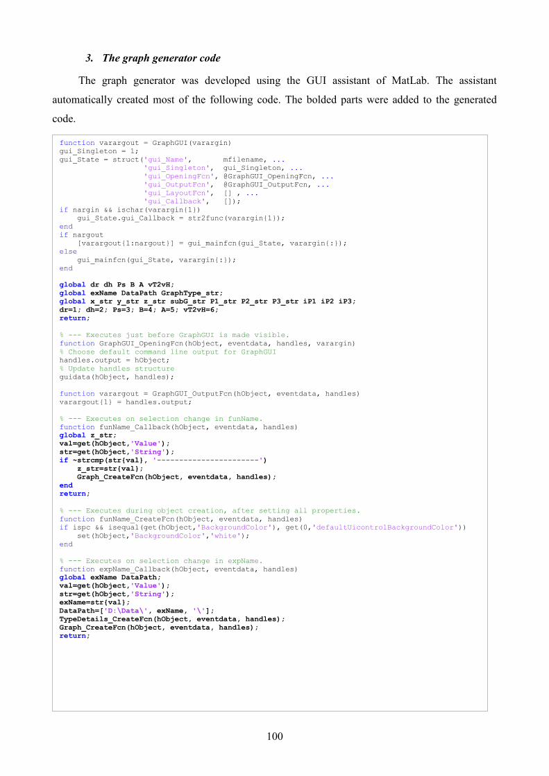
100
3. The graph generator code
The graph generator was developed using the GUI assistant of MatLab. The assistant
automatically created most of the following code. The bolded parts were added to the generated
code.
function varargout = GraphGUI(varargin)
gui_Singleton = 1;
gui_State = struct('gui_Name', mfilename, ...
'gui_Singleton', gui_Singleton, ...
'gui_OpeningFcn', @GraphGUI_OpeningFcn, ...
'gui_OutputFcn', @GraphGUI_OutputFcn, ...
'gui_LayoutFcn', [] , ...
'gui_Callback', []);
if nargin && ischar(varargin{1})
gui_State.gui_Callback = str2func(varargin{1});
end
if nargout
[varargout{1:nargout}] = gui_mainfcn(gui_State, varargin{:});
else
gui_mainfcn(gui_State, varargin{:});
end
global dr dh Ps B A vT2vH;
global exName DataPath GraphType_str;
global x_str y_str z_str subG_str P1_str P2_str P3_str iP1 iP2 iP3;
dr=1; dh=2; Ps=3; B=4; A=5; vT2vH=6;
return;
% --- Executes just before GraphGUI is made visible.
function GraphGUI_OpeningFcn(hObject, eventdata, handles, varargin)
% Choose default command line output for GraphGUI
handles.output = hObject;
% Update handles structure
guidata(hObject, handles);
function varargout = GraphGUI_OutputFcn(hObject, eventdata, handles)
varargout{1} = handles.output;
% --- Executes on selection change in funName.
function funName_Callback(hObject, eventdata, handles)
global z_str;
val=get(hObject,'Value');
str=get(hObject,'String');
if ~strcmp(str{val}, '-----------------------')
z_str=str{val};
Graph_CreateFcn(hObject, eventdata, handles);
end
return;
% --- Executes during object creation, after setting all properties.
function funName_CreateFcn(hObject, eventdata, handles)
if ispc && isequal(get(hObject,'BackgroundColor'), get(0,'defaultUicontrolBackgroundColor'))
set(hObject,'BackgroundColor','white');
end
% --- Executes on selection change in expName.
function expName_Callback(hObject, eventdata, handles)
global exName DataPath;
val=get(hObject,'Value');
str=get(hObject,'String');
exName=str{val};
DataPath=['D:\Data\', exName, '\'];
TypeDetails_CreateFcn(hObject, eventdata, handles);
Graph_CreateFcn(hObject, eventdata, handles);
return;
101
% --- Executes during object creation, after setting all properties.
function expName_CreateFcn(hObject, eventdata, handles)
if ispc && isequal(get(hObject,'BackgroundColor'), get(0,'defaultUicontrolBackgroundColor'))
set(hObject,'BackgroundColor','white');
end
% --- Executes during object creation, after setting all properties.
function TypeDetails_CreateFcn(hObject, eventdata, handles)
global DataPath;
var =['N vH vM vFA vCR vC tr tMotor'];
eval(['load ' DataPath 'Parameters\Parameters.mat ' var])
str={['N=' num2str(N)]; ['vH=' num2str(vH)];['vM=' num2str(vM)];['vFA=' num2str(vFA)];['vCR='
num2str(vCR)];['vC=' num2str(vC)];['tr=' num2str(tr)];['tMotor=' num2str(tMotor)]};
set(handles.TypeDetails,'String', str);
return;
% --- Executes on selection change in axisX.
function axisX_Callback(hObject, eventdata, handles)
global x_str;
val=get(hObject,'Value');
str=get(hObject,'String');
x_str=str{val};
return;
% --- Executes during object creation, after setting all properties.
function axisX_CreateFcn(hObject, eventdata, handles)
if ispc && isequal(get(hObject,'BackgroundColor'), get(0,'defaultUicontrolBackgroundColor'))
set(hObject,'BackgroundColor','white');
end
% --- Executes on selection change in axis_y.
function axisY_Callback(hObject, eventdata, handles)
global y_str;
val=get(hObject,'Value');
str=get(hObject,'String');
y_str=str{val};
return;
% --- Executes during object creation, after setting all properties.
function axisY_CreateFcn(hObject, eventdata, handles)
if ispc && isequal(get(hObject,'BackgroundColor'), get(0,'defaultUicontrolBackgroundColor'))
set(hObject,'BackgroundColor','white');
end
% --- Executes on selection change in axisP1.
function axisP1_Callback(hObject, eventdata, handles)
global P1_str;
val=get(hObject,'Value');
str=get(hObject,'String');
P1_str=str{val};
listP1_CreateFcn(hObject, eventdata, handles);
textP1_CreateFcn(hObject, eventdata, handles);
return;
% --- Executes during object creation, after setting all properties.
function axisP1_CreateFcn(hObject, eventdata, handles)
if ispc && isequal(get(hObject,'BackgroundColor'), get(0,'defaultUicontrolBackgroundColor'))
set(hObject,'BackgroundColor','white');
end
% --- Executes on selection change in axisP2.
function axisP2_Callback(hObject, eventdata, handles)
global P2_str;
val=get(hObject,'Value');
str=get(hObject,'String');
P2_str=str{val};
listP2_CreateFcn(hObject, eventdata, handles);
textP2_CreateFcn(hObject, eventdata, handles);
return;
102
% --- Executes during object creation, after setting all properties.
function axisP2_CreateFcn(hObject, eventdata, handles)
if ispc && isequal(get(hObject,'BackgroundColor'), get(0,'defaultUicontrolBackgroundColor'))
set(hObject,'BackgroundColor','white');
end
% --- Executes on selection change in axisP3.
function axisP3_Callback(hObject, eventdata, handles)
global P3_str;
val=get(hObject,'Value');
str=get(hObject,'String');
P3_str=str{val};
listP3_CreateFcn(hObject, eventdata, handles);
textP3_CreateFcn(hObject, eventdata, handles);
return;
% --- Executes during object creation, after setting all properties.
function axisP3_CreateFcn(hObject, eventdata, handles)
if ispc && isequal(get(hObject,'BackgroundColor'), get(0,'defaultUicontrolBackgroundColor'))
set(hObject,'BackgroundColor','white');
end
% --- Executes on selection change in axisSubG.
function axisSubG_Callback(hObject, eventdata, handles)
global subG_str;
val=get(hObject,'Value');
str=get(hObject,'String');
subG_str=str{val};
return;
% --- Executes during object creation, after setting all properties.
function axisSubG_CreateFcn(hObject, eventdata, handles)
if ispc && isequal(get(hObject,'BackgroundColor'), get(0,'defaultUicontrolBackgroundColor'))
set(hObject,'BackgroundColor','white');
end
% --- Executes on button press in pushbutton1.
function pushbuttonGraph_Callback(hObject, eventdata, handles)
listP1_CreateFcn(hObject, eventdata, handles);
textP1_CreateFcn(hObject, eventdata, handles);
listP2_CreateFcn(hObject, eventdata, handles);
textP2_CreateFcn(hObject, eventdata, handles);
listP3_CreateFcn(hObject, eventdata, handles);
textP3_CreateFcn(hObject, eventdata, handles);
Graph_CreateFcn(hObject, eventdata, handles);
return;
% --- Executes on selection change in listP1.
function listP1_Callback(hObject, eventdata, handles)
global iP1;
iP1=get(hObject,'Value');
Graph_CreateFcn(hObject, eventdata, handles);
return;
% --- Executes during object creation, after setting all properties.
function listP1_CreateFcn(hObject, eventdata, handles)
if ispc && isequal(get(hObject,'BackgroundColor'), get(0,'defaultUicontrolBackgroundColor'))
set(hObject,'BackgroundColor','white');
end
global DataPath;
var =['dr_vector dh_vector Ps_vector B_vector A_vector vT2vH_vector'];
eval(['load ' DataPath 'Parameters\Parameters.mat ' var])
global P1_str;
val=get(handles.axisP1,'Value');
str=get(handles.axisP1,'String');
P1_str=str{val};
vP1=eval([P1_str '_vector']);
list=vP1;
set(handles.listP1,'String', list, 'Value', 1);
return;
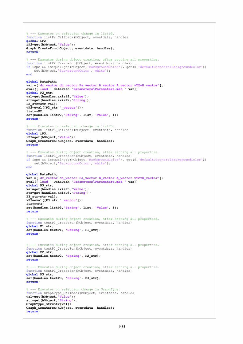
103
% --- Executes on selection change in listP2.
function listP2_Callback(hObject, eventdata, handles)
global iP2;
iP2=get(hObject,'Value');
Graph_CreateFcn(hObject, eventdata, handles);
return;
% --- Executes during object creation, after setting all properties.
function listP2_CreateFcn(hObject, eventdata, handles)
if ispc && isequal(get(hObject,'BackgroundColor'), get(0,'defaultUicontrolBackgroundColor'))
set(hObject,'BackgroundColor','white');
end
global DataPath;
var =['dr_vector dh_vector Ps_vector B_vector A_vector vT2vH_vector'];
eval(['load ' DataPath 'Parameters\Parameters.mat ' var])
global P2_str;
val=get(handles.axisP2,'Value');
str=get(handles.axisP2,'String');
P2_str=str{val};
vP2=eval([P2_str '_vector']);
list=vP2;
set(handles.listP2,'String', list, 'Value', 1);
return;
% --- Executes on selection change in listP3.
function listP3_Callback(hObject, eventdata, handles)
global iP3;
iP3=get(hObject,'Value');
Graph_CreateFcn(hObject, eventdata, handles);
return;
% --- Executes during object creation, after setting all properties.
function listP3_CreateFcn(hObject, eventdata, handles)
if ispc && isequal(get(hObject,'BackgroundColor'), get(0,'defaultUicontrolBackgroundColor'))
set(hObject,'BackgroundColor','white');
end
global DataPath;
var =['dr_vector dh_vector Ps_vector B_vector A_vector vT2vH_vector'];
eval(['load ' DataPath 'Parameters\Parameters.mat ' var])
global P3_str;
val=get(handles.axisP3,'Value');
str=get(handles.axisP3,'String');
P3_str=str{val};
vP3=eval([P3_str '_vector']);
list=vP3;
set(handles.listP3,'String', list, 'Value', 1);
return;
% --- Executes during object creation, after setting all properties.
function textP1_CreateFcn(hObject, eventdata, handles)
global P1_str;
set(handles.textP1, 'String', P1_str);
return;
% --- Executes during object creation, after setting all properties.
function textP2_CreateFcn(hObject, eventdata, handles)
global P2_str;
set(handles.textP2, 'String', P2_str);
return;
% --- Executes during object creation, after setting all properties.
function textP3_CreateFcn(hObject, eventdata, handles)
global P3_str;
set(handles.textP3, 'String', P3_str);
return;
% --- Executes on selection change in GraphType.
function GraphType_Callback(hObject, eventdata, handles)
val=get(hObject,'Value');
str=get(hObject,'String');
GraphType_str=str{val};
Graph_CreateFcn(hObject, eventdata, handles);
return;

104
% --- Executes during object creation, after setting all properties.
function Graph_CreateFcn(hObject, eventdata, handles)
global dr dh Ps B A vT2vH;
global exName DataPath GraphType_str;
global x_str y_str z_str subG_str P1_str P2_str P3_str iP1 iP2 iP3;
% Load the matrix for z cordination
eval(['load ' DataPath 'Optimal\OptimalData.mat ' z_str])
% Load parameters values
var =['dr_vector dh_vector Ps_vector B_vector A_vector vT2vH_vector'];
eval(['load ' DataPath 'Parameters\Parameters.mat ' var])
switch z_str
case 'vT/VI_H'
eval(['load ' DataPath 'Optimal\OptimalData.mat opt_vTs_H opt_VIs_H'])
z=opt_vTs_H./opt_VIs_H;
case 'vT/VI_HR'
eval(['load ' DataPath 'Optimal\OptimalData.mat opt_vTs_HR opt_VIs_HR'])
z=opt_vTs_HR./opt_VIs_HR;
case 'vT/VI_HOR'
eval(['load ' DataPath 'Optimal\OptimalData.mat opt_vTs_HOR opt_VIs_HOR'])
z=opt_vTs_HOR./opt_VIs_HOR;
case 'vT/VI_R'
eval(['load ' DataPath 'Optimal\OptimalData.mat opt_vTs_R opt_VIs_R'])
z=opt_vTs_R./opt_VIs_R;
otherwise
% Load the matrix for z cordination
eval(['load ' DataPath 'Optimal\OptimalData.mat ' z_str])
z=eval(z_str);
end
x=eval(x_str);
y=eval(y_str);
subG=eval(subG_str);
P1=eval(P1_str);
P2=eval(P2_str);
P3=eval(P3_str);
% Rearrange the data matrix
mat=permute(z,[y,x,subG,P1,P2,P3]);
vx=eval([x_str '_vector']);
vy=eval([y_str '_vector']);
vsubG=eval([subG_str '_vector']);
vP1=eval([P1_str '_vector']);
vP2=eval([P2_str '_vector']);
vP3=eval([P3_str '_vector']);
Gname=[ exName ' ' z_str ' X=' x_str ' Y=' y_str ' subG=' subG_str '
' P1_str '=' eval(['num2str(' P1_str '_vector(iP1),2)']) ' ' P2_str '=' eval(['num2str('
P2_str '_vector(iP2),2)']) ' ' P3_str '=' eval(['num2str(' P3_str '_vector(iP3),2)'])];
set(handles.GraphsTitle, 'String', Gname);
hold on
for i=1:6
eval(['h=handles.A' num2str(i) ';'])
reset(h);
set(h,'Visible', 'on');
plot(h,1,1);
set(h,'Visible', 'off');
end
for isubG=1:length(vsubG)
eval(['h=handles.A' num2str(isubG) ';'])
set(h,'Visible', 'on');
if strcmp(z_str, 'opt_CL')
contourf('v6',h,vx,vy,mat(:,:,isubG,iP1,iP2,iP3), [1 2 3 4]);
elseif strcmp(GraphType_str, 'contour')
[C,h1] = contour(h,vx,vy,mat(:,:,isubG,iP1,iP2,iP3));
clabel(C,h1,'FontSize',8);
elseif strcmp(GraphType_str, 'mesh')
mesh(h,vx,vy,mat(:,:,isubG,iP1,iP2,iP3));
end
xlabel(h,x_str);
ylabel(h,y_str);
title(h,[subG_str ' = ' num2str(vsubG(isubG))]);
end
datacursormode on
hold off
return;
%=====================================================================
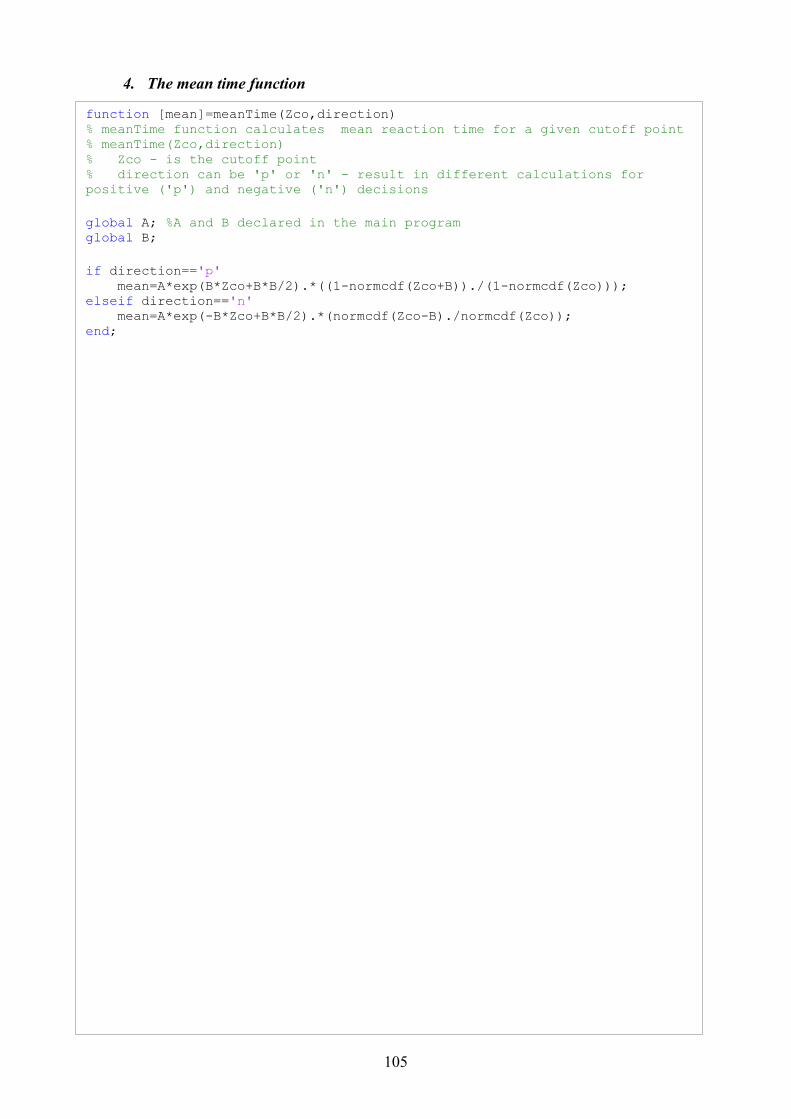
105
4. The mean time function
function [mean]=meanTime(Zco,direction) % meanTime function calculates mean reaction time for a given cutoff point % meanTime(Zco,direction) % Zco - is the cutoff point % direction can be 'p' or 'n' - result in different calculations for
positive ('p') and negative ('n') decisions
global A; %A and B declared in the main program global B;
if direction=='p' mean=A*exp(B*Zco+B*B/2).*((1-normcdf(Zco+B))./(1-normcdf(Zco))); elseif direction=='n' mean=A*exp(-B*Zco+B*B/2).*(normcdf(Zco-B)./normcdf(Zco)); end;

106
107
APPENDIX H - THE RELATION BETWEEN IMAGE COMPLEXITY AND REACTION TIME
Bechar (2006) designed and performed a melon detection experiment in order to examine
different human robot collaboration levels for a specific target detection task in an agriculture
environment. In this work, the experimental data is used to analyze the reaction time of the human
operator. The analysis focuses on the relation between image complexity and reaction time.
1. Melon detection experiment
Full description of the experiment can be found in chapter 6 of Bechar thesis (2006).
Task. The participants of the experiment were asked to detect ready-to-pick melons on a
digital image and mark them on the screen (see example in Figure 36). Some of the participants
fulfilled the task with a help of a robot according to the level of collaboration.
Subjects. 120 IEM undergraduate students were assigned to 10 groups. The participants were
encouraged to achieve high performance through the promise of a monetary award.
Targets database. Melon images were manually selected from a video taken by a camera
moving along a melon row in a field, in various illumination conditions. The melons were partially
covered by leaves and had different colors and sizes. The images were classified into three levels of
complexities (low, intermediate, and high) by a panel of three experts. The image complexity
represents the difficulty level of detecting targets in the image. The location of true targets in each
image was manually identified and saved in a targets database.
Design. In each session, fifteen participants from all experimental groups were seated in a
classroom in front of working stations for target detection that were simulated with a PC and a
program written in MatLab. The participants viewed 180 images, a target was defined as any yellow
or orange melon, and the task was to mark all the targets in the images. The participants were
divided in advance into ten groups, each of which was given one of two objective function weights
(represented by a reward system for minimum false alarm rate or for maximum hit rate), one of two
different robot detection performance qualities, and one of three collaboration levels as shown in
Table 4. In the experiment, the computer simulated the robot operation by picking targets and non-
target objects (marked as false alarms) from the database. The participants received feedback on
their performance during the experiment after each image. The feedback included the current
objective function score (score), the last image number of hits, false alarms and Misses. The
participants had unlimited time to observe the images and the time cost was set to zero.
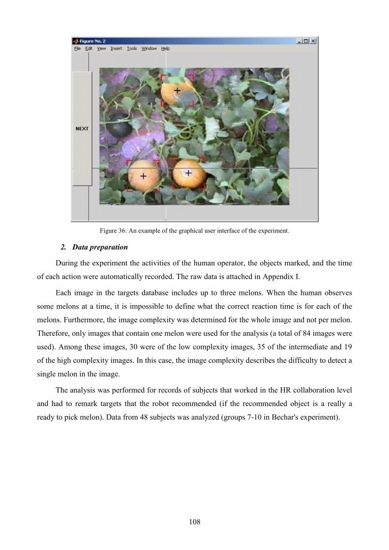
108
Figure 36: An example of the graphical user interface of the experiment.
2. Data preparation
During the experiment the activities of the human operator, the objects marked, and the time
of each action were automatically recorded. The raw data is attached in Appendix I.
Each image in the targets database includes up to three melons. When the human observes
some melons at a time, it is impossible to define what the correct reaction time is for each of the
melons. Furthermore, the image complexity was determined for the whole image and not per melon.
Therefore, only images that contain one melon were used for the analysis (a total of 84 images were
used). Among these images, 30 were of the low complexity images, 35 of the intermediate and 19
of the high complexity images. In this case, the image complexity describes the difficulty to detect a
single melon in the image.
The analysis was performed for records of subjects that worked in the HR collaboration level
and had to remark targets that the robot recommended (if the recommended object is a really a
ready to pick melon). Data from 48 subjects was analyzed (groups 7-10 in Bechar's experiment).
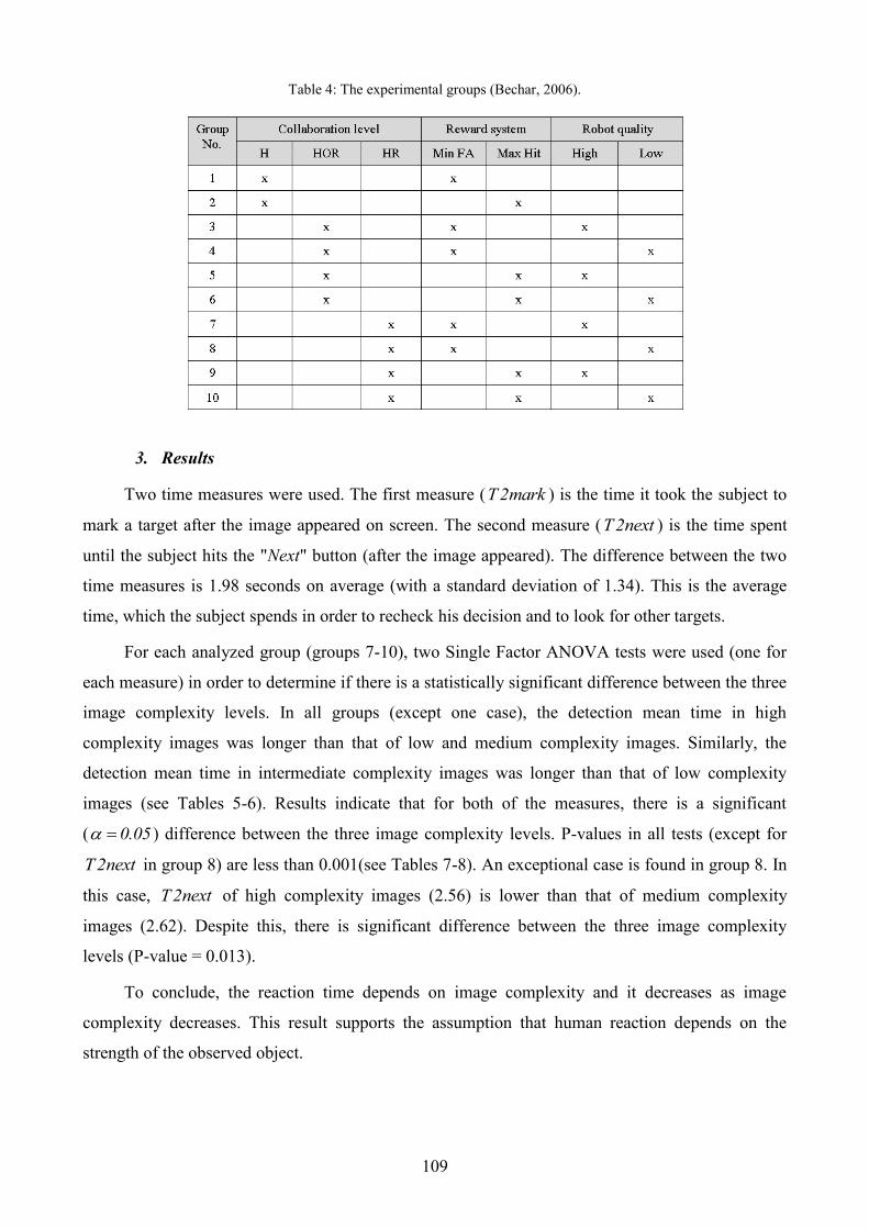
109
Table 4: The experimental groups (Bechar, 2006).
3. Results
Two time measures were used. The first measure (T2mark ) is the time it took the subject to
mark a target after the image appeared on screen. The second measure (T2next ) is the time spent
until the subject hits the "Next" button (after the image appeared). The difference between the two
time measures is 1.98 seconds on average (with a standard deviation of 1.34). This is the average
time, which the subject spends in order to recheck his decision and to look for other targets.
For each analyzed group (groups 7-10), two Single Factor ANOVA tests were used (one for
each measure) in order to determine if there is a statistically significant difference between the three
image complexity levels. In all groups (except one case), the detection mean time in high
complexity images was longer than that of low and medium complexity images. Similarly, the
detection mean time in intermediate complexity images was longer than that of low complexity
images (see Tables 5-6). Results indicate that for both of the measures, there is a significant
( 0.05 ) difference between the three image complexity levels. P-values in all tests (except for
T2next in group 8) are less than 0.001(see Tables 7-8). An exceptional case is found in group 8. In
this case, T2next of high complexity images (2.56) is lower than that of medium complexity
images (2.62). Despite this, there is significant difference between the three image complexity
levels (P-value = 0.013).
To conclude, the reaction time depends on image complexity and it decreases as image
complexity decreases. This result supports the assumption that human reaction depends on the
strength of the observed object.
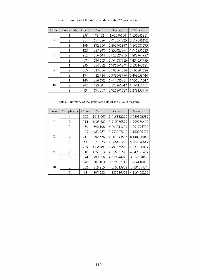
110
Table 5: Summary of the statistical data of the T2mark measure.
Table 6: Summary of the statistical data of the T2next measure.
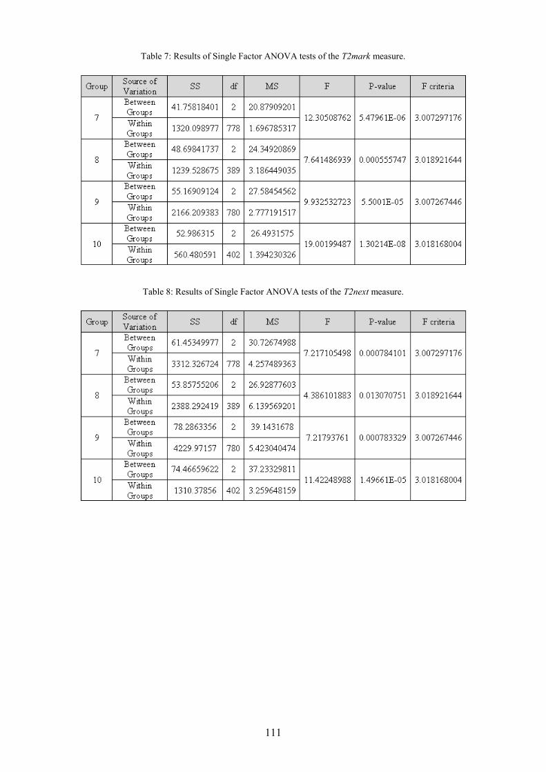
111
Table 7: Results of Single Factor ANOVA tests of the T2mark measure.
Table 8: Results of Single Factor ANOVA tests of the T2next measure.
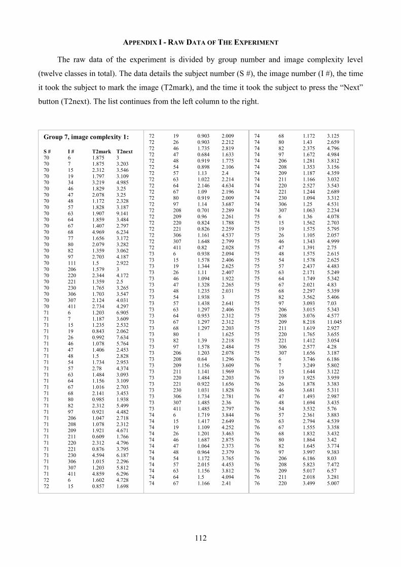
112
APPENDIX I - RAW DATA OF THE EXPERIMENT
The raw data of the experiment is divided by group number and image complexity level
(twelve classes in total). The data details the subject number (S #), the image number (I #), the time
it took the subject to mark the image (T2mark), and the time it took the subject to press the “Next”
button (T2next). The list continues from the left column to the right.
Group 7, image complexity 1:
S # I # T2mark T2next
70 6 1.875 3 70 7 1.875 3.203
70 15 2.312 3.546
70 19 1.797 3.109 70 34 3.219 4.985
70 46 1.829 3.25
70 47 2.078 3.25 70 48 1.172 2.328
70 57 1.828 3.187
70 63 1.907 9.141 70 64 1.859 3.484
70 67 1.407 2.797
70 68 4.969 6.234 70 77 1.656 3.172
70 80 2.079 3.282
70 82 1.359 3.062 70 97 2.703 4.187
70 111 1.5 2.922
70 206 1.579 3 70 220 2.344 4.172
70 221 1.359 2.5
70 230 1.765 3.265 70 306 1.703 3.547
70 307 2.124 4.031 70 411 2.734 4.297
71 6 1.203 6.905
71 7 1.187 3.609 71 15 1.235 2.532
71 19 0.843 2.062
71 26 0.992 7.634 71 46 1.078 5.764
71 47 1.406 2.453
71 48 1.5 2.828 71 54 1.734 2.953
71 57 2.78 4.374
71 63 1.484 3.093 71 64 1.156 3.109
71 67 1.016 2.703
71 68 2.141 3.453 71 80 0.985 1.938
71 82 2.312 5.499
71 97 0.921 4.482 71 206 1.047 2.718
71 208 1.078 2.312
71 209 1.921 4.671 71 211 0.609 1.766
71 220 2.312 4.796
71 221 0.876 3.795 71 230 4.594 6.187
71 306 1.015 2.296
71 307 1.203 5.812
71 411 4.859 6.296
72 6 1.602 4.728
72 15 0.857 1.698
72 19 0.903 2.009
72 26 0.903 2.212
72 46 1.735 2.819 72 47 0.684 1.633
72 48 0.919 1.775
72 54 0.898 2.106 72 57 1.13 2.4
72 63 1.022 2.214
72 64 2.146 4.634 72 67 1.09 2.196
72 80 0.919 2.009
72 97 1.14 3.687 72 208 0.701 2.289
72 209 0.96 2.261
72 220 0.824 1.788 72 221 0.826 2.259
72 306 1.161 4.537
72 307 1.648 2.799 72 411 0.82 2.028
73 6 0.938 2.094
73 15 1.578 2.406
73 19 1.344 2.625
73 26 1.11 2.407
73 46 1.094 1.922 73 47 1.328 2.265
73 48 1.235 2.031 73 54 1.938 3
73 57 1.438 2.641
73 63 1.297 2.406 73 64 0.953 2.312
73 67 1.297 2.312
73 68 1.297 2.203 73 80 1 1.625
73 82 1.39 2.218
73 97 1.578 2.484 73 206 1.203 2.078
73 208 0.64 1.296
73 209 1.156 3.609
73 211 1.141 1.969
73 220 1.484 2.203
73 221 0.922 1.656 73 230 1.031 1.828
73 306 1.734 2.781
73 307 1.485 2.36 73 411 1.485 2.797
74 6 1.719 3.844
74 15 1.417 2.649 74 19 1.109 4.252
74 26 1.201 3.463
74 46 1.687 2.875 74 47 1.064 2.373
74 48 0.964 2.379
74 54 1.172 3.765 74 57 2.015 4.453
74 63 1.156 3.812
74 64 1.5 4.094
74 67 1.166 2.41
74 68 1.172 3.125
74 80 1.43 2.659
74 82 2.375 4.796 74 97 1.672 4.984
74 206 1.281 3.812
74 208 1.353 3.156 74 209 1.187 4.359
74 211 1.166 3.032
74 220 2.527 3.543 74 221 1.244 2.689
74 230 1.094 3.312
74 306 1.25 4.531 74 307 1.063 2.234
75 6 1.36 4.078
75 15 1.562 2.703 75 19 1.575 5.795
75 26 1.105 2.057
75 46 1.343 4.999 75 47 1.391 2.75
75 48 1.575 2.615
75 54 1.578 2.625
75 57 2.437 4.483
75 63 2.171 5.249
75 64 1.749 5.342 75 67 2.021 4.83
75 68 2.297 5.359 75 82 3.562 5.406
75 97 3.093 7.03
75 206 3.015 5.343 75 208 3.076 4.577
75 209 8.218 11.045
75 211 1.619 2.927 75 220 1.765 3.655
75 221 1.412 3.054
75 306 2.577 4.28 75 307 1.656 3.187
76 6 3.746 6.186
76 7 3.249 5.802
76 15 1.644 3.122
76 19 1.925 3.959
76 26 1.878 3.383 76 46 3.681 5.311
76 47 1.493 2.987
76 48 1.694 3.435 76 54 3.532 5.76
76 57 2.361 3.883
76 63 2.794 4.539 76 67 1.555 3.358
76 68 1.832 3.432
76 80 1.864 3.42 76 82 1.645 3.774
76 97 3.997 9.383
76 206 6.186 8.03 76 208 5.823 7.472
76 209 5.017 6.57
76 211 2.018 3.281
76 220 3.499 5.007

113
76 221 1.335 2.825
76 230 2.043 3.462
76 306 4.753 6.242
76 307 1.252 3.092
76 411 2.205 3.634 77 6 1.071 2.461
77 15 0.889 2.452
77 19 1.112 2.002 77 26 0.689 1.722
77 34 0.737 1.64
77 46 7.306 9.611 77 47 1.084 2.878
77 48 0.792 1.626
77 57 2.183 4.916 77 63 1.134 3.524
77 64 1.517 3.601
77 68 3.619 7.483 77 77 1.363 3.16
77 82 3.863 10.261
77 97 1.748 5.896 77 111 1.626 6.764
77 206 1.241 3.969
77 209 1.777 3.355 77 211 0.695 1.599
77 220 1.548 2.851
77 221 1.084 2.516 77 306 2.176 5.777
77 307 1.536 3.833
77 411 4.473 6.046 78 6 0.875 1.859
78 7 0.984 2.203
78 15 1.125 1.922 78 19 0.969 2.172
78 26 0.844 1.719
78 46 0.734 1.828 78 47 0.984 1.828
78 48 0.828 1.781
78 54 0.781 1.687 78 57 1.578 2.797
78 63 0.89 2.078
78 64 0.735 1.672 78 67 0.765 1.765
78 68 1.078 2.156
78 80 0.937 1.703 78 82 0.734 1.734
78 97 1.859 3.094
78 206 0.938 1.953 78 208 0.578 1.828
78 209 1 2.156
78 211 0.89 1.703 78 220 0.657 1.657
78 221 0.765 1.922 78 306 0.828 1.953
78 307 0.922 1.875
78 411 0.984 2.031 79 6 1.044 3.305
79 7 0.997 3.211
79 15 1.294 2.635 79 19 0.952 3.029
79 26 1.078 2.515
79 46 0.699 5.232 79 47 0.966 2.088
79 48 0.89 1.983
79 54 0.543 1.583 79 57 1.025 3.478
79 63 1.134 3.059
79 64 1.31 4.24
79 67 0.733 2.544
79 68 0.9 3.679
79 80 1.124 2.483 79 82 0.901 3.462
79 97 1.297 4.61
79 206 1.107 3.242 79 208 0.749 1.858
79 209 1.195 4.175
79 211 0.64 1.53 79 220 1.013 2.307
79 221 0.78 1.748
79 307 0.827 3.024 79 411 0.962 5.215
7001 6 1.209 2.434
7001 7 1.608 5.587 7001 15 1.377 2.097
7001 19 1.734 3.283
7001 26 1.679 3.136 7001 46 1.437 2.592
7001 47 1.102 2.066
7001 48 1.055 1.762 7001 54 1.762 2.814
7001 57 1.999 3.199
7001 63 1.347 2.725 7001 64 1.857 2.76
7001 67 1.124 1.943
7001 68 1.467 2.518 7001 80 1.52 2.575
7001 82 1.881 2.784
7001 97 2.229 3.411 7001 206 1.111 2.37
7001 208 1.595 2.725
7001 209 1.348 2.503 7001 211 1.203 2.119
7001 220 1.117 2.372
7001 221 1.638 2.498 7001 306 1.422 2.74
7001 307 1.378 2.327
7002 6 0.754 1.715 7002 7 0.842 2.675
7002 15 0.947 1.935
7002 19 0.813 1.788 7002 26 0.765 1.713
7002 34 0.576 1.374
7002 46 2.455 9.022 7002 47 2.868 4.08
7002 48 0.704 1.53
7002 57 1.596 3.084 7002 63 0.96 2.015
7002 64 1.041 2.029 7002 68 6.383 19.579
7002 77 2.571 4.153
7002 82 2.363 9.498 7002 97 3.146 6.215
7002 111 4.232 6.153
7002 206 0.854 1.802 7002 209 0.88 1.855
7002 211 0.754 1.848
7002 220 0.894 1.922 7002 221 0.902 1.774
7002 306 1.041 2.376
7002 307 0.886 2.246 7002 411 3.744 7.153
Group 7, image complexity 2:
S # I # T2mark T2next
70 16 1.734 3.25 70 27 1.5 3.032
70 33 1.859 3.218
70 35 2.593 4.062 70 41 1.984 4.281
70 42 1.297 2.75
70 62 2.188 3.782 70 65 3.14 4.531
70 69 1.406 2.625
70 72 2.188 3.688 70 76 1.937 3.031
70 83 1.032 2.141
70 87 1.734 3.078 70 95 1.969 3.531
70 105 1.844 3.266
70 204 2.609 4.734 70 207 1.86 3.156
70 210 2.438 3.953
70 217 5.703 6.968 70 219 1.375 2.906
70 223 2.016 3.516
70 224 1.078 2.343 70 231 3.859 5.656
70 303 1.656 3.015 70 304 1.516 2.734
70 308 2.547 3.937
70 310 1.906 3.359 70 322 6.89 8.828
70 401 3.421 4.843
71 14 1.312 3.484 71 16 1.765 5.358
71 27 1.312 2.859
71 33 0.672 2.047 71 35 2.061 9.744
71 41 12.547 14.328
71 42 2.562 4.14 71 62 1.922 3.749
71 65 2.781 4.812
71 69 0.781 4.781 71 70 1.094 2.844
71 72 2.156 10.296
71 87 0.812 2.172 71 95 4.803 6.292
71 105 1.296 6.996
71 204 3.64 4.968 71 207 3.489 5.284
71 217 1.906 4.828
71 219 0.938 7.547 71 223 1.031 2.859
71 231 1.639 5.887
71 303 1.219 4.125 71 304 1.016 2.735
71 319 5.294 10.369
71 322 0.921 2.187 72 14 1.121 2.32
72 16 5.173 6.288
72 27 0.929 2.014 72 33 1.059 2.227
72 35 2.657 6.422
72 41 1.106 2.274
72 42 1.259 2.364
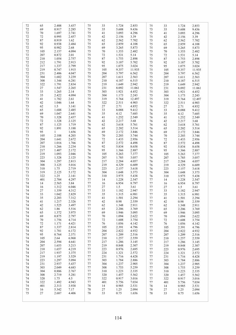
114
72 65 2.488 3.437
72 69 0.917 2.285
72 70 1.697 2.741
72 72 0.995 2.457
72 87 0.919 1.62 72 92 0.938 2.484
72 95 0.982 2.68
72 105 2.157 4.094 72 207 0.872 2.01
72 210 1.054 2.757
72 212 1.791 2.913 72 217 1.337 2.799
72 219 0.747 1.915
72 231 2.406 4.047 72 304 1.682 3.239
72 308 1.344 6.281
72 322 1.791 2.834 73 27 1.547 2.265
73 33 1.265 2.14
73 35 2.422 4.094 73 41 1.782 2.61
73 42 1.046 1.64
73 62 1.5 3.141 73 65 1.688 2.485
73 69 1.047 2.641
73 70 1.328 2.437 73 72 1.328 2.125
73 87 1.125 1.719
73 92 1.891 3.188 73 95 1 1.656
73 105 2.188 4.203
73 204 1.641 2.672 73 207 1.016 1.766
73 210 1.266 2.234
73 217 1.407 2.172 73 219 1.093 2.046
73 223 1.328 2.125
73 304 1.297 2.813 73 308 3.125 5.016
73 310 1.75 2.719
73 319 2.125 5.172 73 322 1.25 2.141
73 401 2.704 4.297
74 14 2.565 3.84 74 16 1.312 6.046
74 27 1.359 4.312
74 33 1.042 2.829 74 35 2.203 7.312
74 41 1.217 2.326
74 42 1.525 3.497 74 62 1.86 5.516
74 65 1.372 3.975 74 69 0.875 2.797
74 70 1.756 4.714
74 72 1.171 4.421 74 87 1.337 2.814
74 92 1.781 6.172
74 95 0.764 2.371 74 105 2.64 6.968
74 204 2.594 4.641
74 207 1.653 3.213 74 210 1.657 4.219
74 217 1.937 3.375
74 219 1.197 3.529 74 223 1.297 5.094
74 231 2.937 5.437
74 303 2.049 4.683 74 304 0.886 2.767
74 308 2.719 5.281
74 320 1.75 4.5
74 322 1.492 4.943
74 401 2.313 3.938
75 16 5.342 7.17
75 27 2.687 4.406
75 33 1.724 2.853
75 35 5.608 9.436
75 41 3.093 4.296
75 42 2.156 3.39
75 62 2.562 7.702 75 65 2.859 4.108
75 69 3.265 5.873
75 70 1.353 2.482 75 72 1.531 5.14
75 87 1.753 2.898
75 92 3.187 5.702 75 95 1.075 3.024
75 105 9.357 11.935
75 204 3.797 6.562 75 207 1.611 2.563
75 210 4.187 6.515
75 219 1.649 2.942 75 231 8.092 11.061
75 303 1.921 4.452
75 304 1.173 2.243 75 319 5.764 12.497
75 322 2.511 4.903
76 27 2.71 4.852 76 33 8.088 9.412
76 35 4.12 7.685
76 41 1.252 2.549 76 42 2.217 3.68
76 62 3.618 5.761
76 65 2.202 3.514 76 69 2.172 3.846
76 70 2.203 3.744
76 72 1.433 2.956 76 87 2.572 4.498
76 92 5.834 8.658
76 95 1.366 2.887 76 105 5.263 7.377
76 207 1.785 3.057
76 217 2.284 4.057 76 219 4.329 6.609
76 223 2.157 3.618
76 304 1.648 3.373 76 310 3.975 5.438
77 14 1.228 2.547
77 16 6.954 8.797 77 27 1.5 3.61
77 33 1.182 2.947
77 35 1.315 6.981 77 41 1.501 2.294
77 42 0.98 2.559
77 62 1.348 2.911 77 65 2.206 3.769
77 69 1.946 3.095 77 70 1.094 2.622
77 72 1.608 3.754
77 76 1.056 4.142 77 105 2.391 4.796
77 204 2.822 4.932
77 207 1.209 2.516 77 210 1.257 2.559
77 217 1.286 3.145
77 219 0.848 2.307 77 223 0.976 2.695
77 224 1.321 2.572
77 231 1.716 4.428 77 303 1.784 2.886
77 304 1.237 2.905
77 308 1.753 5.259 77 310 1.223 2.335
77 320 1.457 5.562
77 322 0.917 3.016
77 401 5.756 7.034
78 14 0.985 2.531
78 27 1.25 2.094
78 33 0.75 1.656
75 33 1.724 2.853 75 35 5.608 9.436
75 41 3.093 4.296
75 42 2.156 3.39 75 62 2.562 7.702
75 65 2.859 4.108
75 69 3.265 5.873 75 70 1.353 2.482
75 72 1.531 5.14
75 87 1.753 2.898 75 92 3.187 5.702
75 95 1.075 3.024
75 105 9.357 11.935 75 204 3.797 6.562
75 207 1.611 2.563
75 210 4.187 6.515 75 219 1.649 2.942
75 231 8.092 11.061
75 303 1.921 4.452
75 304 1.173 2.243
75 319 5.764 12.497
75 322 2.511 4.903 76 27 2.71 4.852
76 33 8.088 9.412
76 35 4.12 7.685 76 41 1.252 2.549
76 42 2.217 3.68 76 62 3.618 5.761
76 65 2.202 3.514
76 69 2.172 3.846 76 70 2.203 3.744
76 72 1.433 2.956
76 87 2.572 4.498 76 92 5.834 8.658
76 95 1.366 2.887
76 105 5.263 7.377
76 207 1.785 3.057
76 217 2.284 4.057
76 219 4.329 6.609 76 223 2.157 3.618
76 304 1.648 3.373
76 310 3.975 5.438 77 14 1.228 2.547
77 16 6.954 8.797
77 27 1.5 3.61 77 33 1.182 2.947
77 35 1.315 6.981
77 41 1.501 2.294 77 42 0.98 2.559
77 62 1.348 2.911
77 65 2.206 3.769 77 69 1.946 3.095
77 70 1.094 2.622
77 72 1.608 3.754 77 76 1.056 4.142
77 105 2.391 4.796
77 204 2.822 4.932 77 207 1.209 2.516
77 210 1.257 2.559
77 217 1.286 3.145 77 219 0.848 2.307
77 223 0.976 2.695
77 224 1.321 2.572 77 231 1.716 4.428
77 303 1.784 2.886
77 304 1.237 2.905 77 308 1.753 5.259
77 310 1.223 2.335
77 320 1.457 5.562 77 322 0.917 3.016
77 401 5.756 7.034
78 14 0.985 2.531 78 27 1.25 2.094
78 33 0.75 1.656

115
78 35 1.625 5.968
78 42 0.891 1.797
78 62 1.843 3.703
78 69 0.875 1.828
78 70 0.843 1.671 78 72 1.328 2.25
78 92 3.328 4.625
78 95 0.891 2.75 78 105 4.843 9.203
78 204 1.422 2.75
78 207 0.938 1.704 78 210 1.015 2.062
78 223 1.094 2.015
78 303 1.203 2.125 78 304 0.875 1.812
78 308 2.047 4.156
78 310 1.531 2.5 78 319 6.469 9.594
78 322 1.11 3.969
78 401 3.015 4.125 79 14 1.296 2.654
79 16 1.738 4.89
79 27 1.273 3.338 79 33 0.765 1.748
79 35 1.703 8.156
79 41 1.217 2.404 79 42 1.496 2.946
79 65 1.699 3.491
79 69 0.92 2.759 79 70 1.155 3.216
79 72 1.215 3.133
79 87 1.467 2.529 79 92 1.593 5.062
79 95 2.296 3.296
79 105 2.281 19.281 79 204 3.819 5.76
79 207 1.53 2.624
79 210 0.947 4.238 79 217 1.434 3.851
79 219 1.03 2.17
79 223 1.263 2.713 79 231 5.234 8.656
79 303 1.045 3.788
79 304 0.889 2.404 79 310 2.92 5.215
79 322 1.14 2.514
79 401 1.422 4.14 7001 14 1.688 2.803
7001 16 2.088 3.302
7001 27 1.748 2.592 7001 33 2.71 3.918
7001 35 3.815 6.716 7001 41 1.286 2.48
7001 42 1.011 2.159
7001 62 1.762 2.962 7001 65 1.194 2.097
7001 69 1.47 2.786
7001 70 1.811 2.725 7001 72 1.041 2.173
7001 87 2.389 3.413
7001 92 2.807 4.5 7001 105 3.895 5.628
7001 204 1.718 3.05
7001 207 2.276 3.706 7001 210 2.355 3.54
7001 217 2.082 2.97
7001 219 1.471 2.555 7001 223 1.378 2.418
7001 231 4.002 5.506
7001 303 1.209 2.541
7001 304 1.416 2.304
7001 308 1.639 2.982
7001 310 3.175 5.73 7001 319 2.928 4.888
7001 320 1.303 2.562
7001 322 2.529 4.188
7001 401 2.78 4.083
7002 14 0.903 1.729
7002 16 3.286 8.184
7002 27 1.134 2.535 7002 33 0.887 1.947
7002 35 2.278 5.611
7002 41 0.887 1.656 7002 42 1.268 2.269
7002 62 0.747 1.534
7002 65 1.562 2.522 7002 69 0.99 2.187
7002 70 0.887 1.729
7002 76 1.478 2.572 7002 87 0.719 1.621
7002 92 5.843 7.145
7002 105 1.015 2.029 7002 204 1.282 2.323
7002 207 0.665 1.611
7002 210 0.92 2.001 7002 217 1.212 2.129
7002 219 0.933 1.912
7002 224 0.734 1.851 7002 231 2.242 4.124
7002 303 0.887 2.01
7002 304 0.734 1.775 7002 308 1.481 2.548
7002 310 0.813 1.715
7002 320 1.626 2.852 7002 322 0.995 1.974
Group 7, image complexity 3:
S # I # T2mark T2next
70 61 3.328 5.109
70 88 3.235 4.969
70 96 4.312 5.843 70 102 4.766 6.391
70 104 2.563 3.907
70 109 1.75 3.218 70 309 2.562 3.781
70 312 1.609 3.468
70 313 4.469 5.938 70 324 1.687 2.812
70 325 1.594 2.781
70 402 2.985 5.578 70 403 2.188 3.438
70 404 2.031 3.484
70 406 2.234 4.109 71 61 1.187 4.953
71 88 1.297 6.749 71 96 4.374 7.217
71 102 1.062 4.841
71 104 1.484 2.562 71 109 1.421 3.249
71 201 2.61 4.875
71 227 1.406 3.796 71 309 5.656 8.843
71 312 0.985 2.906
71 313 2.89 8.67 71 324 1.734 4.5
71 325 0.969 2.359
71 327 3.046 4.53 71 402 8.982 10.498
71 403 2.359 5.093
71 406 1.672 3.515 72 61 1.119 1.85
72 88 0.914 1.967
72 96 0.991 3.36
72 102 2.391 6.079
72 104 3.567 4.719
72 227 1.58 2.804 72 309 1.223 2.679
72 312 0.996 1.868
72 313 1.843 4.863
72 324 2.177 3.25
72 325 1.028 1.916
72 403 1.137 3.037
72 406 1.368 2.784 73 61 1.157 1.969
73 88 1.593 2.468
73 96 2.078 3.344 73 102 4 5.234
73 201 1.593 2.39
73 227 1.297 2.187 73 309 1.891 2.75
73 312 1.562 2.906
73 324 1.61 2.532 73 325 1.704 2.375
73 327 5.234 6.421
73 402 1.922 3.062 73 403 1.515 2.359
74 61 3.066 4.314
74 88 2.124 5.859 74 96 1.703 6.046
74 102 4.015 6.578
74 104 2.296 3.775 74 109 3.405 5.299
74 201 1.648 3.342
74 227 1.578 4.765 74 309 1.781 4.64
74 312 1.197 3.218
74 313 3.5 8.188 74 324 2.634 4.205
74 325 1.555 3.202
74 327 3.672 5.562 74 402 1.703 7.891
74 403 1.679 3.235
75 61 2.124 3.296 75 88 6.186 7.951
75 96 5.202 6.827
75 102 6.342 10.404 75 109 2.312 4.062
75 201 2.243 3.462
75 227 1.718 4.749 75 312 1.501 3.136
75 313 8.076 10.451
75 324 2.375 4.187 75 325 2.021 4.859
75 402 5.671 11.014
75 403 1.594 2.844 76 227 3.675 5.562
76 312 5.06 6.442
76 324 3.092 5.415 76 325 4.098 5.469
76 403 1.885 3.303 76 406 2.986 4.253
77 61 1.778 3.724
77 88 2.51 7.694 77 96 1.517 4.03
77 102 5.287 8.472
77 104 1.363 3.37 77 109 1.44 2.743
77 201 2.187 3.64
77 227 2.298 5.348 77 309 3.551 5.021
77 312 0.974 2.112
77 313 3.417 6.236 77 324 1.001 3.114
77 325 1.633 3.25
77 327 1.648 6.952 77 402 2.198 7.873
77 404 1.251 3.42
78 61 0.828 1.781
78 88 1.344 2.485
78 104 1.219 3.016
78 109 0.953 1.797 78 201 1.375 3.39
78 227 1.344 2.625
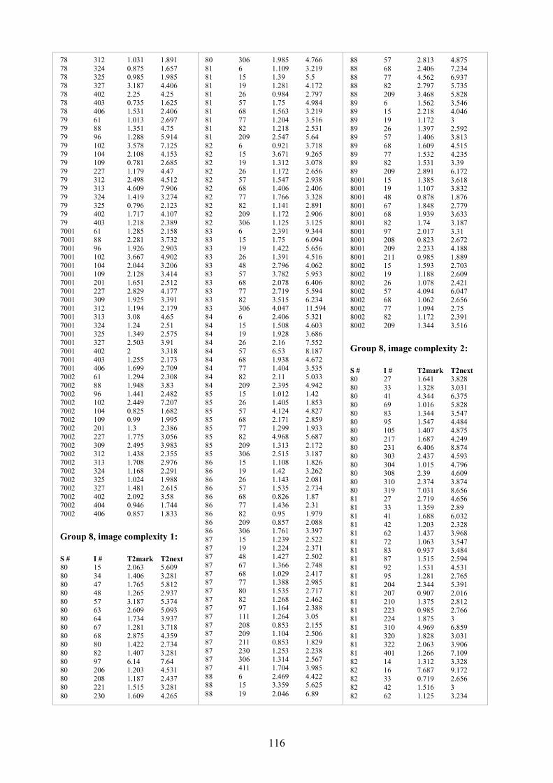
116
78 312 1.031 1.891
78 324 0.875 1.657
78 325 0.985 1.985
78 327 3.187 4.406
78 402 2.25 4.25 78 403 0.735 1.625
78 406 1.531 2.406
79 61 1.013 2.697 79 88 1.351 4.75
79 96 1.288 5.914
79 102 3.578 7.125 79 104 2.108 4.153
79 109 0.781 2.685
79 227 1.179 4.47 79 312 2.498 4.512
79 313 4.609 7.906
79 324 1.419 3.274 79 325 0.796 2.123
79 402 1.717 4.107
79 403 1.218 2.389 7001 61 1.285 2.158
7001 88 2.281 3.732
7001 96 1.926 2.903 7001 102 3.667 4.902
7001 104 2.044 3.206
7001 109 2.128 3.414 7001 201 1.651 2.512
7001 227 2.829 4.177
7001 309 1.925 3.391 7001 312 1.194 2.179
7001 313 3.08 4.65
7001 324 1.24 2.51 7001 325 1.349 2.575
7001 327 2.503 3.91
7001 402 2 3.318 7001 403 1.255 2.173
7001 406 1.699 2.709
7002 61 1.294 2.308 7002 88 1.948 3.83
7002 96 1.441 2.482
7002 102 2.449 7.207 7002 104 0.825 1.682
7002 109 0.99 1.995
7002 201 1.3 2.386 7002 227 1.775 3.056
7002 309 2.495 3.983
7002 312 1.438 2.355 7002 313 1.708 2.976
7002 324 1.168 2.291
7002 325 1.024 1.988 7002 327 1.481 2.615
7002 402 2.092 3.58 7002 404 0.946 1.744
7002 406 0.857 1.833
Group 8, image complexity 1:
S # I # T2mark T2next
80 15 2.063 5.609
80 34 1.406 3.281
80 47 1.765 5.812 80 48 1.265 2.937
80 57 3.187 5.374
80 63 2.609 5.093 80 64 1.734 3.937
80 67 1.281 3.718
80 68 2.875 4.359 80 80 1.422 2.734
80 82 1.407 3.281
80 97 6.14 7.64 80 206 1.203 4.531
80 208 1.187 2.437
80 221 1.515 3.281
80 230 1.609 4.265
80 306 1.985 4.766
81 6 1.109 3.219
81 15 1.39 5.5
81 19 1.281 4.172
81 26 0.984 2.797 81 57 1.75 4.984
81 68 1.563 3.219
81 77 1.204 3.516 81 82 1.218 2.531
81 209 2.547 5.64
82 6 0.921 3.718 82 15 3.671 9.265
82 19 1.312 3.078
82 26 1.172 2.656 82 57 1.547 2.938
82 68 1.406 2.406
82 77 1.766 3.328 82 82 1.141 2.891
82 209 1.172 2.906
82 306 1.125 3.125 83 6 2.391 9.344
83 15 1.75 6.094
83 19 1.422 5.656 83 26 1.391 4.516
83 48 2.796 4.062
83 57 3.782 5.953 83 68 2.078 6.406
83 77 2.719 5.594
83 82 3.515 6.234 83 306 4.047 11.594
84 6 2.406 5.321
84 15 1.508 4.603 84 19 1.928 3.686
84 26 2.16 7.552
84 57 6.53 8.187 84 68 1.938 4.672
84 77 1.404 3.535
84 82 2.11 5.033 84 209 2.395 4.942
85 15 1.012 1.42
85 26 1.405 1.853 85 57 4.124 4.827
85 68 2.171 2.859
85 77 1.299 1.933 85 82 4.968 5.687
85 209 1.313 2.172
85 306 2.515 3.187 86 15 1.108 1.826
86 19 1.42 3.262
86 26 1.143 2.081 86 57 1.535 2.734
86 68 0.826 1.87 86 77 1.436 2.31
86 82 0.95 1.979
86 209 0.857 2.088 86 306 1.761 3.397
87 15 1.239 2.522
87 19 1.224 2.371 87 48 1.427 2.502
87 67 1.366 2.748
87 68 1.029 2.417 87 77 1.388 2.985
87 80 1.535 2.717
87 82 1.268 2.462 87 97 1.164 2.388
87 111 1.264 3.05
87 208 0.853 2.155 87 209 1.104 2.506
87 211 0.853 1.829
87 230 1.253 2.238
87 306 1.314 2.567
87 411 1.704 3.985
88 6 2.469 4.422 88 15 3.359 5.625
88 19 2.046 6.89
88 57 2.813 4.875
88 68 2.406 7.234
88 77 4.562 6.937 88 82 2.797 5.735
88 209 3.468 5.828
89 6 1.562 3.546 89 15 2.218 4.046
89 19 1.172 3
89 26 1.397 2.592 89 57 1.406 3.813
89 68 1.609 4.515
89 77 1.532 4.235 89 82 1.531 3.39
89 209 2.891 6.172
8001 15 1.385 3.618 8001 19 1.107 3.832
8001 48 0.878 1.876
8001 67 1.848 2.779 8001 68 1.939 3.633
8001 82 1.74 3.187
8001 97 2.017 3.31 8001 208 0.823 2.672
8001 209 2.233 4.188
8001 211 0.985 1.889 8002 15 1.593 2.703
8002 19 1.188 2.609
8002 26 1.078 2.421 8002 57 4.094 6.047
8002 68 1.062 2.656
8002 77 1.094 2.75 8002 82 1.172 2.391
8002 209 1.344 3.516
Group 8, image complexity 2:
S # I # T2mark T2next
80 27 1.641 3.828
80 33 1.328 3.031 80 41 4.344 6.375
80 69 1.016 5.828
80 83 1.344 3.547 80 95 1.547 4.484
80 105 1.407 4.875
80 217 1.687 4.249 80 231 6.406 8.874
80 303 2.437 4.593
80 304 1.015 4.796 80 308 2.39 4.609
80 310 2.374 3.874
80 319 7.031 8.656 81 27 2.719 4.656
81 33 1.359 2.89
81 41 1.688 6.032 81 42 1.203 2.328
81 62 1.437 3.968
81 72 1.063 3.547 81 83 0.937 3.484
81 87 1.515 2.594
81 92 1.531 4.531 81 95 1.281 2.765
81 204 2.344 5.391
81 207 0.907 2.016 81 210 1.375 2.812
81 223 0.985 2.766 81 224 1.875 3
81 310 4.969 6.859
81 320 1.828 3.031 81 322 2.063 3.906
81 401 1.266 7.109
82 14 1.312 3.328 82 16 7.687 9.172
82 33 0.719 2.656
82 42 1.516 3
82 62 1.125 3.234
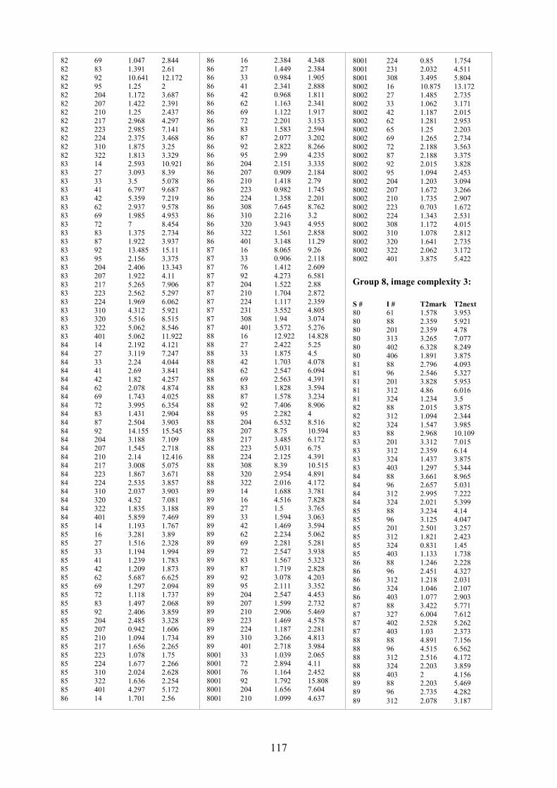
117
82 69 1.047 2.844
82 83 1.391 2.61
82 92 10.641 12.172 82 95 1.25 2
82 204 1.172 3.687
82 207 1.422 2.391 82 210 1.25 2.437
82 217 2.968 4.297
82 223 2.985 7.141 82 224 2.375 3.468
82 310 1.875 3.25
82 322 1.813 3.329 83 14 2.593 10.921
83 27 3.093 8.39
83 33 3.5 5.078 83 41 6.797 9.687
83 42 5.359 7.219
83 62 2.937 9.578 83 69 1.985 4.953
83 72 7 8.454
83 83 1.375 2.734 83 87 1.922 3.937
83 92 13.485 15.11
83 95 2.156 3.375 83 204 2.406 13.343
83 207 1.922 4.11
83 217 5.265 7.906 83 223 2.562 5.297
83 224 1.969 6.062
83 310 4.312 5.921 83 320 5.516 8.515
83 322 5.062 8.546
83 401 5.062 11.922 84 14 2.192 4.121
84 27 3.119 7.247
84 33 2.24 4.044
84 41 2.69 3.841
84 42 1.82 4.257
84 62 2.078 4.874 84 69 1.743 4.025
84 72 3.995 6.354 84 83 1.431 2.904
84 87 2.504 3.903
84 92 14.155 15.545 84 204 3.188 7.109
84 207 1.545 2.718
84 210 2.14 12.416 84 217 3.008 5.075
84 223 1.867 3.671
84 224 2.535 3.857 84 310 2.037 3.903
84 320 4.52 7.081
84 322 1.835 3.188
84 401 5.859 7.469
85 14 1.193 1.767
85 16 3.281 3.89 85 27 1.516 2.328
85 33 1.194 1.994
85 41 1.239 1.783 85 42 1.209 1.873
85 62 5.687 6.625
85 69 1.297 2.094 85 72 1.118 1.737
85 83 1.497 2.068
85 92 2.406 3.859 85 204 2.485 3.328
85 207 0.942 1.606
85 210 1.094 1.734 85 217 1.656 2.265
85 223 1.078 1.75
85 224 1.677 2.266 85 310 2.024 2.628
85 322 1.636 2.254
85 401 4.297 5.172
86 14 1.701 2.56
86 16 2.384 4.348
86 27 1.449 2.384
86 33 0.984 1.905
86 41 2.341 2.888
86 42 0.968 1.811 86 62 1.163 2.341
86 69 1.122 1.917
86 72 2.201 3.153 86 83 1.583 2.594
86 87 2.077 3.202
86 92 2.822 8.266 86 95 2.99 4.235
86 204 2.151 3.335
86 207 0.909 2.184 86 210 1.418 2.79
86 223 0.982 1.745
86 224 1.358 2.201 86 308 7.645 8.762
86 310 2.216 3.2
86 320 3.943 4.955 86 322 1.561 2.858
86 401 3.148 11.29
87 16 8.065 9.26 87 33 0.906 2.118
87 76 1.412 2.609
87 92 4.273 6.581 87 204 1.522 2.88
87 210 1.704 2.872
87 224 1.117 2.359 87 231 3.552 4.805
87 308 1.94 3.074
87 401 3.572 5.276 88 16 12.922 14.828
88 27 2.422 5.25
88 33 1.875 4.5 88 42 1.703 4.078
88 62 2.547 6.094
88 69 2.563 4.391 88 83 1.828 3.594
88 87 1.578 3.234
88 92 7.406 8.906 88 95 2.282 4
88 204 6.532 8.516
88 207 8.75 10.594 88 217 3.485 6.172
88 223 5.031 6.75
88 224 2.125 4.391 88 308 8.39 10.515
88 320 2.954 4.891
88 322 2.016 4.172 89 14 1.688 3.781
89 16 4.516 7.828 89 27 1.5 3.765
89 33 1.594 3.063
89 42 1.469 3.594 89 62 2.234 5.062
89 69 2.281 5.281
89 72 2.547 3.938 89 83 1.567 5.323
89 87 1.719 2.828
89 92 3.078 4.203 89 95 2.111 3.352
89 204 2.547 4.453
89 207 1.599 2.732 89 210 2.906 5.469
89 223 1.469 4.578
89 224 1.187 2.281 89 310 3.266 4.813
89 401 2.718 3.984
8001 33 1.039 2.065
8001 72 2.894 4.11
8001 76 1.164 2.452
8001 92 1.792 15.808 8001 204 1.656 7.604
8001 210 1.099 4.637
8001 224 0.85 1.754 8001 231 2.032 4.511
8001 308 3.495 5.804
8002 16 10.875 13.172 8002 27 1.485 2.735
8002 33 1.062 3.171
8002 42 1.187 2.015 8002 62 1.281 2.953
8002 65 1.25 2.203
8002 69 1.265 2.734 8002 72 2.188 3.563
8002 87 2.188 3.375
8002 92 2.015 3.828 8002 95 1.094 2.453
8002 204 1.203 3.094
8002 207 1.672 3.266 8002 210 1.735 2.907
8002 223 0.703 1.672
8002 224 1.343 2.531
8002 308 1.172 4.015
8002 310 1.078 2.812
8002 320 1.641 2.735 8002 322 2.062 3.172
8002 401 3.875 5.422
Group 8, image complexity 3:
S # I # T2mark T2next
80 61 1.578 3.953
80 88 2.359 5.921 80 201 2.359 4.78
80 313 3.265 7.077
80 402 6.328 8.249 80 406 1.891 3.875
81 88 2.796 4.093
81 96 2.546 5.327 81 201 3.828 5.953
81 312 4.86 6.016
81 324 1.234 3.5 82 88 2.015 3.875
82 312 1.094 2.344
82 324 1.547 3.985 83 88 2.968 10.109
83 201 3.312 7.015
83 312 2.359 6.14 83 324 1.437 3.875
83 403 1.297 5.344
84 88 3.661 8.965 84 96 2.657 5.031
84 312 2.995 7.222 84 324 2.021 5.399
85 88 3.234 4.14
85 96 3.125 4.047 85 201 2.501 3.257
85 312 1.821 2.423
85 324 0.831 1.45 85 403 1.133 1.738
86 88 1.246 2.228
86 96 2.451 4.327 86 312 1.218 2.031
86 324 1.046 2.107
86 403 1.077 2.903 87 88 3.422 5.771
87 327 6.004 7.612
87 402 2.528 5.262 87 403 1.03 2.373
88 88 4.891 7.156
88 96 4.515 6.562
88 312 2.516 4.172
88 324 2.203 3.859
88 403 2 4.156 89 88 2.203 5.469
89 96 2.735 4.282
89 312 2.078 3.187
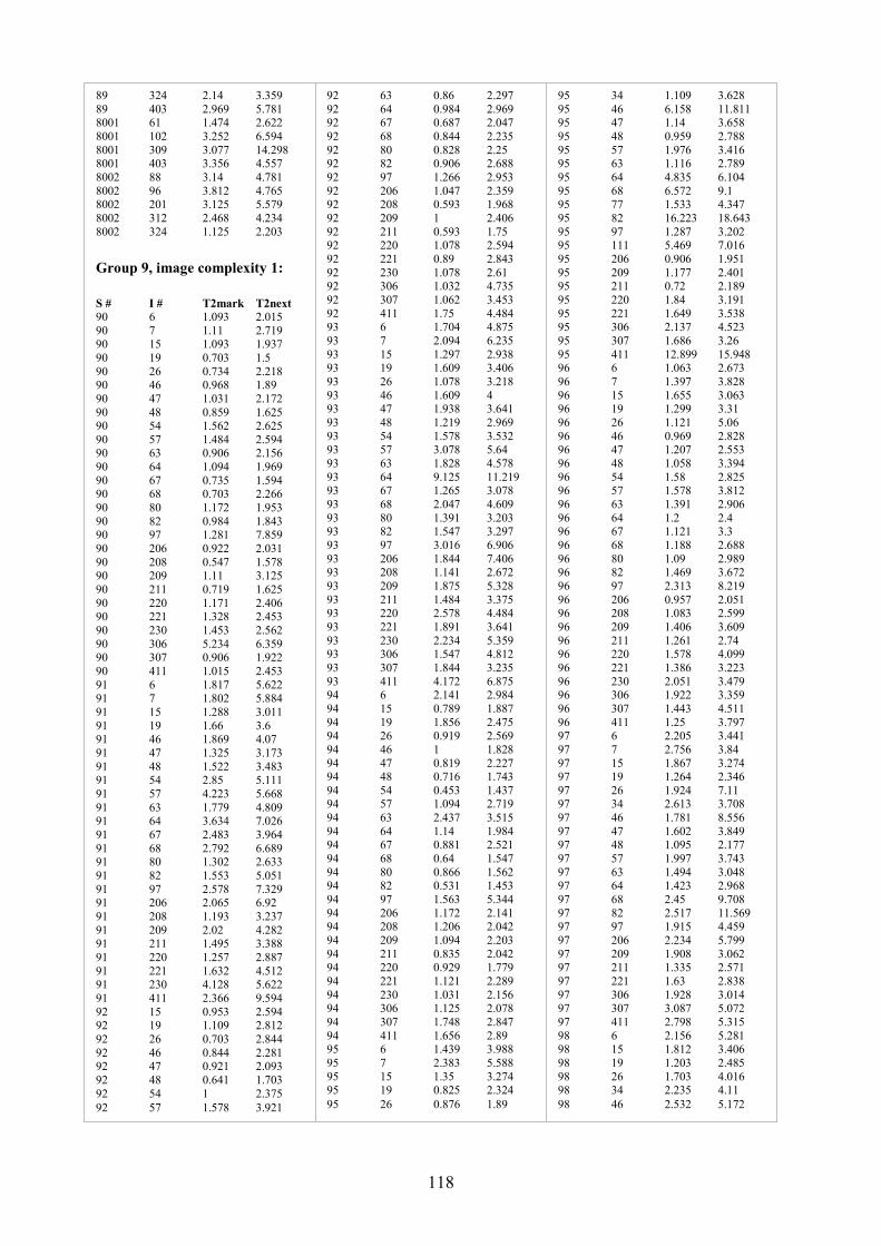
118
89 324 2.14 3.359
89 403 2.969 5.781
8001 61 1.474 2.622
8001 102 3.252 6.594
8001 309 3.077 14.298 8001 403 3.356 4.557
8002 88 3.14 4.781
8002 96 3.812 4.765 8002 201 3.125 5.579
8002 312 2.468 4.234
8002 324 1.125 2.203
Group 9, image complexity 1:
S # I # T2mark T2next
90 6 1.093 2.015
90 7 1.11 2.719
90 15 1.093 1.937
90 19 0.703 1.5
90 26 0.734 2.218 90 46 0.968 1.89
90 47 1.031 2.172
90 48 0.859 1.625 90 54 1.562 2.625
90 57 1.484 2.594 90 63 0.906 2.156
90 64 1.094 1.969
90 67 0.735 1.594 90 68 0.703 2.266
90 80 1.172 1.953
90 82 0.984 1.843 90 97 1.281 7.859
90 206 0.922 2.031
90 208 0.547 1.578
90 209 1.11 3.125
90 211 0.719 1.625
90 220 1.171 2.406 90 221 1.328 2.453
90 230 1.453 2.562
90 306 5.234 6.359 90 307 0.906 1.922
90 411 1.015 2.453
91 6 1.817 5.622 91 7 1.802 5.884
91 15 1.288 3.011
91 19 1.66 3.6 91 46 1.869 4.07
91 47 1.325 3.173
91 48 1.522 3.483 91 54 2.85 5.111
91 57 4.223 5.668
91 63 1.779 4.809 91 64 3.634 7.026
91 67 2.483 3.964
91 68 2.792 6.689 91 80 1.302 2.633
91 82 1.553 5.051
91 97 2.578 7.329 91 206 2.065 6.92
91 208 1.193 3.237
91 209 2.02 4.282 91 211 1.495 3.388
91 220 1.257 2.887
91 221 1.632 4.512 91 230 4.128 5.622
91 411 2.366 9.594
92 15 0.953 2.594 92 19 1.109 2.812
92 26 0.703 2.844
92 46 0.844 2.281 92 47 0.921 2.093
92 48 0.641 1.703
92 54 1 2.375
92 57 1.578 3.921
92 63 0.86 2.297
92 64 0.984 2.969
92 67 0.687 2.047
92 68 0.844 2.235
92 80 0.828 2.25 92 82 0.906 2.688
92 97 1.266 2.953
92 206 1.047 2.359 92 208 0.593 1.968
92 209 1 2.406
92 211 0.593 1.75 92 220 1.078 2.594
92 221 0.89 2.843
92 230 1.078 2.61 92 306 1.032 4.735
92 307 1.062 3.453
92 411 1.75 4.484 93 6 1.704 4.875
93 7 2.094 6.235
93 15 1.297 2.938 93 19 1.609 3.406
93 26 1.078 3.218
93 46 1.609 4 93 47 1.938 3.641
93 48 1.219 2.969
93 54 1.578 3.532 93 57 3.078 5.64
93 63 1.828 4.578
93 64 9.125 11.219 93 67 1.265 3.078
93 68 2.047 4.609
93 80 1.391 3.203 93 82 1.547 3.297
93 97 3.016 6.906
93 206 1.844 7.406 93 208 1.141 2.672
93 209 1.875 5.328
93 211 1.484 3.375 93 220 2.578 4.484
93 221 1.891 3.641
93 230 2.234 5.359 93 306 1.547 4.812
93 307 1.844 3.235
93 411 4.172 6.875 94 6 2.141 2.984
94 15 0.789 1.887
94 19 1.856 2.475 94 26 0.919 2.569
94 46 1 1.828
94 47 0.819 2.227 94 48 0.716 1.743
94 54 0.453 1.437 94 57 1.094 2.719
94 63 2.437 3.515
94 64 1.14 1.984 94 67 0.881 2.521
94 68 0.64 1.547
94 80 0.866 1.562 94 82 0.531 1.453
94 97 1.563 5.344
94 206 1.172 2.141 94 208 1.206 2.042
94 209 1.094 2.203
94 211 0.835 2.042 94 220 0.929 1.779
94 221 1.121 2.289
94 230 1.031 2.156 94 306 1.125 2.078
94 307 1.748 2.847
94 411 1.656 2.89
95 6 1.439 3.988
95 7 2.383 5.588
95 15 1.35 3.274 95 19 0.825 2.324
95 26 0.876 1.89
95 34 1.109 3.628
95 46 6.158 11.811
95 47 1.14 3.658
95 48 0.959 2.788
95 57 1.976 3.416 95 63 1.116 2.789
95 64 4.835 6.104
95 68 6.572 9.1 95 77 1.533 4.347
95 82 16.223 18.643
95 97 1.287 3.202 95 111 5.469 7.016
95 206 0.906 1.951
95 209 1.177 2.401 95 211 0.72 2.189
95 220 1.84 3.191
95 221 1.649 3.538 95 306 2.137 4.523
95 307 1.686 3.26
95 411 12.899 15.948 96 6 1.063 2.673
96 7 1.397 3.828
96 15 1.655 3.063 96 19 1.299 3.31
96 26 1.121 5.06
96 46 0.969 2.828 96 47 1.207 2.553
96 48 1.058 3.394
96 54 1.58 2.825 96 57 1.578 3.812
96 63 1.391 2.906
96 64 1.2 2.4 96 67 1.121 3.3
96 68 1.188 2.688
96 80 1.09 2.989 96 82 1.469 3.672
96 97 2.313 8.219
96 206 0.957 2.051 96 208 1.083 2.599
96 209 1.406 3.609
96 211 1.261 2.74 96 220 1.578 4.099
96 221 1.386 3.223
96 230 2.051 3.479 96 306 1.922 3.359
96 307 1.443 4.511
96 411 1.25 3.797 97 6 2.205 3.441
97 7 2.756 3.84
97 15 1.867 3.274 97 19 1.264 2.346
97 26 1.924 7.11 97 34 2.613 3.708
97 46 1.781 8.556
97 47 1.602 3.849 97 48 1.095 2.177
97 57 1.997 3.743
97 63 1.494 3.048 97 64 1.423 2.968
97 68 2.45 9.708
97 82 2.517 11.569 97 97 1.915 4.459
97 206 2.234 5.799
97 209 1.908 3.062 97 211 1.335 2.571
97 221 1.63 2.838
97 306 1.928 3.014 97 307 3.087 5.072
97 411 2.798 5.315
98 6 2.156 5.281
98 15 1.812 3.406
98 19 1.203 2.485
98 26 1.703 4.016 98 34 2.235 4.11
98 46 2.532 5.172

119
98 47 1.578 2.922
98 48 1.125 2.593
98 54 1.812 4.609
98 57 2.891 5.578
98 63 3.297 5.109 98 64 1.578 4.265
98 67 1.984 3.469
98 68 2.61 5.734 98 80 1.093 2.14
98 82 1.86 4.219
98 97 2.484 5.968 98 206 2.594 4.766
98 208 1.031 2.422
98 209 2.203 4.844 98 220 6.281 7.874
98 230 2.235 3.797
98 307 2.109 3.531 99 6 1.421 2.859
99 7 1.734 3.843
99 15 1.686 2.698 99 19 1.962 3.081
99 26 4.64 6.177
99 46 1.672 2.547 99 47 1.548 2.53
99 48 1.738 3.026
99 54 1.609 2.89 99 57 2.344 4.375
99 63 3.047 5.625
99 64 2.187 3.859 99 67 2.079 3.181
99 68 2.609 4.89
99 80 2.701 3.926 99 82 2.906 4.75
99 97 5.359 8.593
99 206 1.172 2.531 99 208 2.023 2.943
99 209 1.703 3.156
99 211 0.947 1.63 99 220 1.426 2.576
99 221 1.769 2.964
99 230 1.64 3 99 306 1.953 3.156
99 307 1.226 2.437
99 411 2.672 4.563 9001 6 0.953 2.656
9001 15 1.11 2.844
9001 19 1.422 2.984 9001 26 1.219 2.562
9001 47 1.515 3.187
9001 48 1.234 2.406 9001 54 0.89 2.359
9001 63 1.64 3.5 9001 64 1.391 2.86
9001 67 1.016 2.797
9001 68 1.469 4.875 9001 80 1.532 3.141
9001 97 1.5 6.453
9001 206 1.265 2.953 9001 208 0.766 2.704
9001 211 1.062 2.625
9001 220 1.703 3.156 9001 221 1.187 2.453
9001 230 1.375 2.812
9001 307 1.281 4.547 9002 6 1.812 5.671
9002 7 2.391 5.188
9002 15 1.609 3.5 9002 19 1.391 3.25
9002 26 1.204 3.703
9002 46 1.265 4.312
9002 47 1.313 2.937
9002 48 1.5 3.219
9002 54 1.766 3.156 9002 57 1.547 4.203
9002 63 1.859 4.281
9002 64 1.515 5.093
9002 67 2.063 3.625
9002 68 2.109 4.093
9002 80 1.547 3.406
9002 82 2.016 3.985 9002 97 2.469 6.765
9002 206 2.125 4.172
9002 208 1.625 3.703 9002 209 1.781 4.047
9002 211 1.265 6.75
9002 220 2.047 3.922 9002 221 1.453 3.562
9002 230 2.218 4.703
9002 307 1.89 5.124 9002 411 2.828 7.047
Group 9, image complexity 2:
S # I # T2mark T2next
90 14 1.312 2.312 90 16 2.625 4.203
90 27 1.219 2.235
90 33 0.765 1.562 90 35 5.25 7.047
90 41 1 1.75 90 42 1.14 1.953
90 62 0.735 1.703
90 70 1.125 2.39 90 87 2.687 3.562
90 92 1.5 3.047
90 95 2.391 3.625 90 105 3.797 7.297
90 204 1.344 2.516
90 207 0.687 2.015
90 210 1.031 2.687
90 219 0.781 1.796
90 223 0.938 2 90 231 2.766 7.344
90 303 1.125 2.469
90 304 0.797 1.672 90 319 3.063 6.672
90 320 1.406 2.656
90 322 1.094 2.032 90 401 2.375 3.672
91 14 1.92 4.114
91 16 5.925 10.81 91 27 2.201 4.101
91 33 1.399 4.512
91 35 5.877 12.062 91 41 1.35 2.592
91 42 1.602 5.622
91 62 3.444 5.825 91 69 3.481 5.083
91 70 1.676 4.361
91 72 3.111 4.436 91 87 1.289 2.674
91 92 2.205 7.562
91 105 8.946 18.432 91 204 2.664 5.966
91 210 1.824 2.985
91 217 1.787 4.421 91 219 1.577 3.662
91 223 2.433 5.037
91 231 4.86 8.292 91 303 1.878 3.601
91 304 2.084 3.62
91 319 4.472 14.379 91 320 1.553 4.011
91 322 1.399 4.32
91 401 7.455 9.297 92 14 0.859 2.765
92 16 1.906 4.062
92 27 1.219 3.079
92 33 0.687 2.047
92 35 1.531 3.344
92 41 0.937 2.484
92 42 0.907 2.297
92 62 1.031 3.422
92 65 1.11 2.5 92 69 0.891 2.141
92 70 0.89 2.593
92 72 3.453 5.235 92 87 0.922 2.438
92 92 3.031 4.39
92 95 0.734 2.343 92 105 1.281 2.843
92 204 1.266 3.672
92 207 0.719 2.203 92 210 1.016 2.61
92 217 1.109 2.609
92 219 0.688 2.359 92 223 0.922 2.375
92 303 0.828 2.281
92 304 0.781 2.39 92 310 1.125 3.156
92 319 2.328 3.828
92 322 0.922 3.063 92 401 3.172 4.828
93 14 1.641 3.516
93 16 6.563 8.36 93 27 1.765 3.828
93 33 1.547 3.297
93 35 3.578 8 93 41 1.735 3.204
93 42 1.766 3.078
93 62 3.593 5.703 93 65 2.297 6
93 69 3.297 5.078
93 70 1.422 3.172 93 87 3.157 5.25
93 92 9 10.969
93 95 1.547 4.937 93 105 2.063 6.703
93 204 2.875 6.172
93 207 1.64 3.297 93 210 2.156 4.109
93 217 3.516 5.328
93 219 1.594 3.875 93 223 2.281 3.828
93 231 14.203 16.625
93 303 3.015 4.343 93 304 1.359 2.687
93 319 12.11 13.641
93 322 2.219 4.875 93 401 7.765 9.593
94 14 1.609 2.414 94 27 1.063 2.109
94 33 0.68 1.485
94 35 4.718 7.093 94 41 0.851 1.779
94 42 0.82 1.763
94 62 1.203 3.407 94 65 0.735 2
94 69 0.703 1.359
94 70 0.728 1.64 94 72 0.61 1.188
94 87 0.696 1.237
94 92 1.656 3.281 94 105 2.562 5.781
94 204 1.469 2.578
94 207 0.934 1.899 94 210 0.891 2.047
94 217 0.843 1.484
94 219 2.073 3.559
94 223 0.906 1.703
94 231 3.749 5.031
94 303 1.161 2.445 94 304 0.638 1.51
94 308 1.562 4.406
120
94 310 1.918 2.955
94 320 0.891 1.766
94 322 1.098 2.367
94 401 1.343 3.515
95 14 0.968 2.29 95 16 2.436 3.616
95 27 3.432 4.703
95 33 1.229 2.699 95 35 4.886 6.189
95 41 1.394 2.519
95 42 1.184 2.215 95 62 1.163 2.746
95 69 0.975 2.034
95 70 0.795 1.719 95 76 1.739 5.742
95 87 3.073 4.077
95 92 2.574 4.075 95 105 1.843 3.872
95 204 1.487 3.082
95 207 0.974 2.278 95 210 1.599 4.221
95 219 0.885 2.114
95 223 2.021 3.108 95 224 0.96 1.994
95 231 4.492 8.427
95 303 1.421 3.595 95 304 1.17 2.489
95 308 0.96 2.014
95 320 2.327 5.769 95 322 1.154 2.308
96 14 1.454 2.862
96 16 6.765 11.5 96 27 1.218 3.749
96 33 1.16 4.811
96 35 3.078 7.562 96 41 2.398 4.177
96 42 1.368 3.859
96 62 1.5 3.156 96 65 1.686 3.296
96 69 1.23 3.357
96 70 0.959 2.645 96 72 1.503 3.19
96 87 4.733 9.389
96 92 5.391 7.141 96 95 1.432 3.02
96 105 2.36 7.781
96 204 2.374 4.968 96 207 1.494 3.736
96 210 1.216 3.707
96 217 1.929 3.251 96 219 1.16 3.279
96 223 1.23 2.749 96 231 5.296 9.937
96 303 2.119 5.058
96 304 1.37 2.942 96 319 4.266 9.984
96 322 5.584 8.368
96 401 2.828 4.969 97 14 1.549 2.571
97 16 1.62 5.717
97 27 3.003 4.009 97 33 2.641 4.636
97 35 1.339 4.231
97 41 2.557 3.779 97 42 1.515 2.968
97 62 1.79 2.831
97 65 2.417 4.835 97 69 4.254 5.769
97 70 1.579 2.556
97 87 1.684 2.736
97 105 3.611 6.519
97 204 2.367 3.521
97 207 1.587 3.202 97 210 1.775 3.091
97 217 2.246 3.469
97 219 1.63 2.599
97 223 2.353 5.388
97 224 1.475 2.388
97 303 3.189 4.335
97 304 1.32 2.5 97 310 1.404 2.57
97 322 1.924 3.067
98 16 4.781 7.203 98 27 3.672 7.688
98 33 1.656 3.953
98 41 1.735 3.516 98 42 2.218 4.39
98 62 3.969 6.797
98 69 1.641 4.079 98 70 1.281 3.187
98 72 1.938 3.61
98 76 1.781 3.719 98 83 1.047 2.531
98 95 1.219 2.906
98 105 4.375 7.485 98 204 4.094 6.688
98 207 1.485 2.875
98 210 1.734 4.063 98 217 2.687 3.984
98 219 1.344 3.125
98 223 1.656 4.203 98 224 1.297 3.234
98 231 2.578 6.031
98 303 3.109 6.234 98 304 1.313 2.297
98 308 4.672 6
98 319 3.141 4.75 98 322 1.485 2.797
98 401 4 5.078
99 27 1.828 3.844 99 33 1.947 2.852
99 35 3.547 6.469
99 41 1.487 2.668 99 42 1.272 2.361
99 65 1.375 2.578
99 69 2.031 3.25 99 70 2.759 5.335
99 72 1.063 2.25
99 87 2.499 3.588 99 95 3.538 4.655
99 105 3.64 6.25
99 204 2.593 3.937 99 207 1.567 2.653
99 210 7.422 11.031
99 219 2.116 3.189 99 223 1.89 3.14
99 304 1.676 2.839 99 310 2.238 4.017
99 319 4.656 6.531
99 320 1.812 3.218 99 322 1.536 2.809
99 401 3.156 5.203
9001 14 1.031 2.406 9001 27 1.39 3.875
9001 33 1.234 2.734
9001 41 2.016 3.5 9001 65 1.609 3.547
9001 72 1.015 2.515
9001 87 2.11 3.969 9001 95 1.734 3.453
9001 105 5.296 7.796
9001 207 1.36 2.61 9001 210 3.593 5.343
9001 217 1.157 2.719
9001 219 1.188 3.125
9001 223 1.157 2.86
9001 303 1.375 3.187
9001 304 1.016 2.469 9001 320 1.016 3.156
9001 322 1.313 3.485
9001 401 1.125 5.593
9002 14 1.922 4.453
9002 16 2.812 8.89
9002 27 1.922 4.421
9002 33 1.344 3.656 9002 35 5.688 8.125
9002 41 4.781 6.64
9002 42 1.641 5.485 9002 62 1.938 3.344
9002 65 3 4.485
9002 69 2.25 4.75 9002 70 1.515 6.624
9002 72 1.625 4.89
9002 87 1.562 3.453 9002 92 3.125 5.812
9002 95 1.406 3.844
9002 105 4.687 8.421 9002 207 1.485 3.282
9002 210 1.797 4.219
9002 219 1.781 5.469 9002 223 1.515 6.25
9002 231 4.812 8.546
9002 303 15.25 17.359 9002 304 1.859 3.422
9002 308 8.234 12.891
9002 310 1.39 3.781 9002 319 8.359 12.593
9002 320 2.062 4.047
9002 322 2.422 5.875 9002 401 4.766 7.61
Group 9, image complexity 3:
S # I # T2mark T2next
90 88 1.656 2.781
90 96 1.797 2.828
90 102 1.766 5.094 90 104 1.75 2.703
90 109 1.046 2.156
90 201 1.14 2.328 90 227 1.14 2.328
90 312 0.891 1.938
90 324 3.766 4.922 90 325 1.015 1.984
90 327 1.031 3.781
90 402 4.969 6.391 90 403 1.172 2.469
90 406 1.953 3.031
91 61 2.522 5.176 91 88 2.744 8.548
91 96 3.387 6.533
91 102 2.889 6.771 91 104 1.94 5.183
91 109 3.135 4.936
91 201 2.277 3.936 91 227 1.673 5.261
91 309 5.653 8.669
91 312 1.686 3.524 91 313 2.919 7.156
91 324 2.557 4.482
91 325 1.427 4.43 91 327 1.956 17.176
91 402 2.013 8.503
91 403 2.67 4.299 92 61 0.828 2.313
92 88 1.281 3.14
92 96 1.344 2.797 92 102 2.281 3.703
92 104 1.11 3.453
92 109 1.563 3.344 92 201 1.094 2.609
92 227 1.172 2.812
92 309 1.313 3.141
92 312 0.953 2.547
121
92 313 4.328 5.859
92 324 0.844 2.344
92 325 1.016 4.016
92 327 2.296 5.124
92 402 1.328 3.047 92 403 0.797 2.984
92 406 0.937 2.406
93 61 2.281 4.015 93 88 2.703 4.547
93 96 3.532 5.125
93 102 4.985 7.203 93 104 2.812 4.89
93 109 2.25 4.141
93 201 2.157 4.031 93 227 2.015 4.359
93 309 3.328 5.125
93 312 1.391 4.531 93 324 1.734 3.781
93 325 2.187 3.781
93 327 2.89 6.546 93 402 6.891 8.75
93 403 2.219 4.094
93 406 3.672 5.531 94 61 0.773 1.485
94 88 0.765 1.859
94 96 1.328 2.953 94 102 2.469 3.641
94 104 1.299 2.382
94 109 1.037 2.476 94 227 0.922 1.813
94 309 0.891 1.735
94 312 0.887 1.744 94 313 1.735 3.047
94 324 0.906 1.547
94 325 0.851 1.485 94 327 2.188 3.266
94 402 1.531 2.656
94 403 1.238 2.939 94 406 1.609 3.435
95 88 1.272 2.758
95 96 2.014 3.424 95 104 1.999 3.167
95 109 1.951 3.846
95 201 1.921 4.32 95 227 2.633 3.966
95 309 1.623 5.576
95 324 3.283 4.363 95 325 0.922 3.305
95 327 1.828 2.835
95 404 1.245 2.624 96 61 1.454 3.171
96 88 1.437 2.875 96 96 1.937 5.265
96 102 1.766 4.75
96 104 6.992 8.538 96 109 1.671 4.161
96 227 1.5 5.219
96 309 1.359 3.171 96 312 1.448 3.736
96 313 2.359 4.218
96 324 1.169 2.628 96 325 1.377 3.604
96 327 1.5 5.437
96 402 2.187 5.875 96 403 1.516 4.068
96 406 2.278 3.904
97 61 1.362 2.586 97 88 8.67 10.712
97 96 3.106 4.621
97 102 3.307 5.771
97 104 6.87 8.704
97 109 2.923 5.432
97 227 2.188 3.703 97 309 2.16 4.439
97 312 1.669 2.751
97 313 3.259 4.957
97 324 2.023 3.161
97 325 1.488 2.48
97 327 1.776 4.794
97 402 4.143 5.149 97 404 2.15 3.793
97 406 2.137 3.562
98 61 2.593 5.281 98 88 3.735 5.594
98 96 2.25 5.422
98 102 7.281 11.156 98 104 2 3.422
98 227 4.171 7.765
98 309 4.219 7.375 98 312 1.813 3.407
98 313 3.766 6.094
98 325 1.969 4.016 98 327 4.25 6.735
98 402 6.531 8.765
98 403 1.594 3.25 98 404 1.266 2.547
99 88 5.484 7.109
99 109 6.746 8.202 99 201 1.785 3.089
99 227 2.531 3.843
99 312 1.987 3.104 99 324 1.453 2.828
99 325 3.072 4.174
99 402 3.921 5.327 99 403 1.549 3.741
9001 61 1.656 3.062
9001 88 2.203 5.797 9001 96 1.562 6.015
9001 102 9.016 10.906
9001 104 1.89 3.718 9001 109 3.5 4.828
9001 201 1.813 4
9001 227 1.328 5.359 9001 309 1.125 4.203
9001 312 1.359 2.953
9001 324 1.469 3.313 9001 325 1.437 3.281
9001 403 2.047 4.172
9001 406 1.187 2.656 9002 61 4.156 5.969
9002 88 2.203 6.656
9002 96 4.985 7.172 9002 102 2.859 9.172
9002 104 1.375 4.141
9002 109 1.234 3.468 9002 227 2.172 3.828
9002 309 1.531 8.312 9002 312 1.938 6.469
9002 313 5.562 7.468
9002 324 1.703 4.218 9002 325 1.766 4.797
9002 327 3.172 7.297
9002 402 6.109 7.703 9002 406 4.218 8.859
Group 10, image complexity 1:
S # I # T2mark T2next
100 15 2.047 4.125 100 34 0.954 2.532
100 46 1.968 3.921
100 47 1.437 2.593 100 48 0.922 2.156
100 57 3.89 5.718
100 63 1.25 2.906 100 64 1.469 2.656
100 68 1.609 4.078
100 80 1.093 2.515
100 82 1.734 4.891
100 97 1.375 2.906
100 206 1.265 2.953
100 208 1.609 3.859
100 209 1.719 5.922
100 220 1.766 3.656 100 221 1.281 2.515
100 230 1.25 2.593
100 411 1.375 5.109 101 6 1.611 2.477
101 15 1.215 2.021
101 19 0.957 1.838 101 26 1.041 1.802
101 57 2.48 4.177
101 68 1.378 3.118 101 77 1.763 3.237
101 82 1.16 2.349
101 209 1.653 3.988 101 306 1.32 2.422
102 15 0.875 1.86
102 34 2.079 3.094 102 46 1.063 2.766
102 47 1.219 5.625
102 48 1.094 2.36 102 57 3.985 5.782
102 63 0.843 2.156
102 64 1.797 3.141 102 67 0.906 1.953
102 68 1.422 2.5
102 80 0.781 2.203 102 82 1.281 2.953
102 97 1.047 2.828
102 111 1.234 3.218 102 206 0.765 2.39
102 208 0.766 1.922
102 209 1.5 2.766 102 220 1.578 4.156
102 221 1.063 6.094
102 306 1.359 3.859 103 6 1.687 5.141
103 15 1.547 4.344
103 19 2.25 7.313 103 26 1.438 2.938
103 68 2.172 5.563
103 77 1.625 3.172 103 82 2.703 3.968
103 306 1.953 5.797
104 6 1.796 2.89 104 15 1.094 2.313
104 19 4.843 5.875
104 26 1.771 2.828 104 57 1.484 2.937
104 68 2.938 3.922 104 77 1.375 2.859
104 82 1.437 2.578
104 209 2.797 4.156 104 306 1.094 2.719
105 6 1.937 8.906
105 15 1 2.641 105 19 1.047 2.422
105 26 0.922 6.094
105 57 1.157 3.235 105 68 0.969 4.25
105 77 1.938 3.891
105 82 1.031 5.156 105 209 1 3.266
106 15 1.798 5.815
106 26 1.221 2.769 106 34 0.953 3.626
106 46 2.511 4.814
106 47 1.183 3.38
106 48 1.845 2.917
106 57 2.14 3.323
106 63 1.812 2.83 106 64 4.621 5.862
106 67 1.519 3.603
122
106 68 1.197 1.991
106 77 1.798 3.826
106 206 1.426 2.822
106 208 1.282 2.674
106 209 1.123 2.261 106 221 1.419 3.288
106 411 1.901 4.102
107 26 1.203 3.047 107 57 1.25 4.938
107 68 1.5 5.312
107 82 2.703 4.593 107 209 1.687 4.078
107 306 1.812 4.781
108 15 1.5 3.485 108 34 1.125 1.922
108 47 3.031 4.859
108 54 1.625 2.39 108 57 2.438 5
108 63 1.797 3.5
108 64 1.672 3.672 108 68 1.437 4.703
108 206 1.578 3.89
108 208 1.172 2.031 108 411 2.094 4.016
109 6 1.016 2.172
109 15 0.781 1.813 109 19 1.188 2.219
109 26 0.86 1.735
109 57 1.047 3.203 109 68 1.141 2.266
109 77 1.172 2.781
109 82 1.125 1.922 109 306 1.312 2.281
110 6 1.297 3.797
110 15 1.047 2.672 110 19 1.281 3.687
110 26 1.265 3.078
110 57 1.703 4.125 110 68 1.063 4.266
110 77 1.485 3.391
110 82 2.5 4.906 110 209 1.391 3.391
110 306 4.266 7.469
111 15 7.186 9.812 111 46 3.577 5.344
111 48 1.383 2.588
111 68 2.042 3.609 111 77 1.783 3.767
111 80 1.055 2.41
111 82 1.797 3.133 111 97 2.15 4.131
111 208 1.029 2.504 111 209 2.411 4.039
111 211 1.193 2.639
Group 10, image complexity 2:
S # I # T2mark T2next
100 27 1.563 2.969
100 33 1.734 4.875
100 41 1.156 2.578 100 69 1.156 2.656
100 72 1.672 3.812
100 83 1.203 2.578 100 87 1.375 3.156
100 105 1.187 3.047
100 204 1.532 4.407 100 217 3.109 4.812
100 223 1.594 3.016
100 310 1.313 2.766 101 14 1.992 3.151
101 16 4.961 7.485
101 27 1.334 2.741
101 33 1.498 2.78
101 41 1.991 2.812
101 42 1.322 2.036
101 62 1.944 4.496
101 69 0.912 1.611
101 72 0.972 3.617 101 83 1.103 1.724
101 87 1.127 2.286
101 92 6.607 7.987 101 95 1.228 2.004
101 105 5.226 6.854
101 204 1.74 4.467 101 207 1.43 2.098
101 210 1.175 2.335
101 223 1.261 2.522 101 224 1.189 2.224
102 33 1.25 2.516
102 69 1.125 2.484 102 72 2.219 3.984
102 83 2.578 3.875
102 87 1.14 2.953 102 95 1.422 2.579
102 105 1.625 2.812
102 204 1.609 3.218 102 217 1.578 3.594
102 223 4.063 5.688
102 231 3.359 5.516 102 303 1.735 3.156
102 304 0.984 4.874
102 308 4.062 5.656 102 310 1.062 2.484
103 14 2.313 4.875
103 16 4.797 8.453 103 27 1.704 4.297
103 33 2.937 4.125
103 42 2.75 6.468 103 62 4.734 11.391
103 69 2.203 4.719
103 83 1.484 3.312 103 92 5.985 9.516
103 95 4.062 5.687
103 204 5.141 14.953 103 207 2.172 3.437
103 210 1.657 5.75
103 217 2.86 4.61 103 223 2.063 3.438
103 224 3.968 5.375
103 308 5.672 9.782 103 310 4.5 5.766
104 14 1.219 2.781
104 16 2.938 4.188 104 27 2.204 3.891
104 33 1.187 2.094 104 42 1.531 2.828
104 62 1.703 3.156
104 69 1.297 2.484 104 72 1.875 2.922
104 83 2.952 4.568
104 92 2.157 4.094 104 95 1.849 2.781
104 204 2.063 4.032
104 207 1.29 2.455 104 210 1.438 3.86
104 223 1.546 2.703
104 224 1.25 2.281 104 310 3.641 5.016
104 322 1.249 2.718
105 14 1.578 9.031 105 16 2.688 10.656
105 27 1.219 4.985
105 33 0.906 2.5
105 41 3.125 4.296
105 42 1.156 2.734
105 62 2 6.141 105 69 1.625 4.344
105 72 1.328 2.687
105 83 0.719 1.781
105 87 1.25 2.75
105 95 1.312 3.734
105 204 2.938 4.86
105 207 2.125 3.453 105 210 1.312 5.875
105 217 5.141 6.922
105 223 1.453 3.156 105 224 1.546 5.984
105 308 5.671 10.296
105 310 2.266 3.891 105 320 6.078 7.484
105 322 1.282 5.469
105 401 3.859 6.219 106 16 2.186 4.177
106 33 1.787 2.756
106 41 1.706 2.827 106 42 1.768 4.063
106 62 1.647 2.56
106 65 1.613 6.311 106 69 1.429 2.75
106 72 2.781 4.364
106 83 1.324 2.115 106 87 1.76 2.524
106 204 3.009 3.892
106 207 2.674 5.512 106 219 1.474 2.754
106 223 1.121 1.843
106 231 1.97 4.357 106 303 1.429 2.243
106 310 2.879 3.684
106 319 4.717 5.55 106 320 3.994 5.392
106 322 1.515 4.407
107 14 1.578 3.89 107 16 5.093 8.578
107 27 1.204 4.422
107 33 1.125 2.797 107 41 2.5 4.171
107 42 1.781 2.797
107 72 1.219 3.078 107 83 0.984 1.859
107 87 0.813 1.579
107 92 3.344 5.953 107 95 1.109 3.171
107 207 1.14 2.156
107 210 1.187 3.422 107 223 2.25 3.36
107 224 1.188 2.141
107 308 3.469 6 107 310 1.141 2.578
107 320 1.828 3.687 107 401 3.781 5.094
108 14 3.609 5.515
108 92 1.718 6.218 108 95 1.078 2.093
108 204 3 3.875
108 207 1.703 3.593 108 223 1.656 3.609
108 224 3.297 4.047
108 401 4.25 6.016 109 27 1.359 2.219
109 33 1.125 5.5
109 41 0.969 2.625 109 42 1.547 2.438
109 62 1.125 3.75
109 72 2.359 3.281 109 83 1.906 2.734
109 87 0.907 1.86
109 92 1.64 2.968
109 95 1.016 2.219
109 204 1.532 2.703
109 207 1.218 2.093 109 210 1.016 1.969
109 223 0.812 1.75
123
109 224 1.016 2
109 308 2.656 5.078
109 310 1.25 2.203
109 320 0.828 1.75
109 322 1.297 3.516 109 401 2.078 4.344
110 14 6.516 8.047
110 16 2.187 5.406 110 27 2.547 4.593
110 33 1.218 3.343
110 41 1.172 3.453 110 42 2.25 4.828
110 62 1.656 4.187
110 69 1.594 3.907 110 72 1.329 3.438
110 83 1.265 2.547
110 87 2.109 3.39 110 95 1.204 2.813
110 204 4.765 8.046
110 207 1.562 3.641 110 210 1.172 4.781
110 217 2.094 3.734
110 223 1.235 3.61 110 224 1.547 2.907
110 310 2.578 3.812
110 322 2.063 4.11 110 401 2.125 4.11
111 33 1.63 4.012
111 76 1.177 2.67 111 92 3.342 4.585
111 210 3.931 5.71
111 224 1.058 2.251 111 231 4.315 5.636
111 308 2.78 3.854
111 320 2.666 4.449 111 401 2.085 5.22
Group 10, image complexity 3:
S # I # T2mark T2next
100 61 2.375 3.75
100 88 1.813 9.828
100 96 2.703 6.219 100 201 3.953 5.531
100 402 5.469 6.938
100 406 2.281 3.469 101 88 2.597 4.178
101 96 3.158 6.425
101 312 1.035 2.611 101 324 1.17 1.793
101 403 1.282 2.394
102 61 1.141 3.422 102 96 2.343 3.968
102 201 2.5 6.265
102 402 3.188 5.188 103 88 5.531 8.375
103 201 6.359 12.234
103 312 6.203 7.562 103 324 1.469 2.906
104 88 2.125 3.969
104 96 2.578 3.937 104 324 2.094 3.157
104 403 1.828 3.766
105 88 2.016 6.61 105 96 5.547 7.141
105 201 2.078 9.516
105 312 2.344 4.625 105 324 1.36 3.204
105 403 1.968 4.171
106 61 2.822 4.885 106 96 2.305 3.982
106 102 2.317 5.674
106 104 2.51 4.12
106 109 1.444 4.102
106 309 2.575 3.458
106 312 4.032 6.173
106 324 2.295 4.589
106 327 7.007 7.812
106 403 1.368 2.996 107 88 7.703 8.75
107 96 3.734 4.844
107 201 4.312 5.234 107 312 1.297 2.188
107 324 1.828 2.89
108 96 3.046 4.562 108 325 1.828 3.469
108 402 3.187 6.405
108 403 1.203 2.797 108 404 1.563 4.109
109 88 3.282 4.391
109 96 1.079 3.328 109 201 2.484 4.265
109 312 2.39 3.64
109 324 3.594 4.328 109 403 1.281 3.016
110 88 1.875 4.578
110 96 2.688 7.454 110 201 3.484 5.406
110 312 1.687 3.562
110 324 1.172 2.891 110 403 1.719 4.156
111 88 3.466 5.261
111 403 2.672 5.221

תקציר
שילוב מפעיל אנושי . פועלים בסביבות דינאמיות ובלתי מובנותמוגבלים בבצועיהם כאשר הם רובוטים אוטונומיים
מערכות שיתוף פעולה בין אדם לרובוט . הפחתת מורכבות המערכתללשיפור הביצועים ו יכול לתרוםבמערכת רובוטית
ניתן ליישם שיתוף פעולה ברמות . וק והעקביות של הרובוטה של האדם כמו גם מהדיסמפיקות תועלת מיכולות התפי
. שונות הנבדלות בניהן ברמת האוטונומיה של הרובוט
פיתוח קודם של פונקצית מתבססת עלההערכה . רובוט-אדם משולבתתיזה זו מתמקדת בהערכת מערכת זיהוי מטרות
. לה הוגדרו במיוחד עבור משימת זיהוי מטרותארבע רמות שיתוף פעו(. 2006, בכר)מטרה עבור משימת זיהוי מטרות
הסביבה והמשימה באמצעות , האדם, פונקצית המטרה של המודל מכמתת את השפעת הפרמטרים השונים של הרובוט
. המודל מאפשר לקבוע מהי רמת שיתוף הפעולה האופטימאלית בהינתן פרמטרים אלו. סכום משוקלל של מדדי ביצוע
זמן התגובה משפיע על . הזמן הדרוש לאדם כדי להחליט האם אובייקט הוא מטרה או לאזמן התגובה של האדם הוא
עבודה זו מציגה המשך פיתוח של פונקצית המטרה ולוקחת בחשבון שזמן התגובה תלוי . עלויות התפעול של המערכת
ובה המבוסס על מודל של מודל זמן תג, במחקר זה. זמן שאינו קבוע בין אובייקטים, בעוצמת האות של האובייקט הנבחן
המודל החדש צפוי לתאר מערכות אמיתיות בצורה טובה יותר על . (2006) משולב לתוך המודל של בכר( 1985)מורדוק
מטרת המחקר היא להעריך את השפעת זמן התגובה של האדם . ידי התאמת הפרמטרים של פונקצית הזמן למשימה מוגדרת
. מיטבייםפעת זמן התגובה על רמת שיתוף הפעולה שמניבה את הביצועים ההמחקר מתמקד בהש. על ביצועי המערכת
ברמות שיתוף . הניתוחים מגלים רמות שיתוף פעולה חדשות אשר מועדפות כאשר עלות זמן התגובה של האדם גבוהה
האדם עלות זמן התגובה של, כתוצאה מכך. ומתעלם מאחרים חלק מהאובייקטים רק האדם מתמקד בבחינת, פעולה אלה
. האדם מתעלם מאובייקטים על ידי קביעת סף ההחלטה שלו לערך קיצוני. יורד והמערכת מציגה ביצועים טובים יותר
משפיעים על , ההסתברות של אובייקט להיות מטרה ועלות הזמן, רגישות האדם, הניתוחים מראים כיצד סוג המערכת
. תופעת בחירת ערך סף קיצוני
שכאשר המערכת נותנת , הניתוחים מראים. כאשר רגישות האדם נמוכה יכולת ההבחנה שלו בין מטרות לרעש יורדת
אשר גורם לכך שאף אובייקט לא מסומן כמטרה , האדם בוחר ערך סף קיצוני חיובי, עדיפות גבוהה למניעת התראות שווא
אשר , לא להחטיא מטרות נבחר ערך סף קיצוני שליליבמערכת אשר נותנת עדיפות גבוהה . ולא מתרחשות התראות שווא
תופעה זו מופיעה עבור רגישויות גבוהות . גורם לכך שכל האובייקטים מסומנים כמטרות ומכאן שכל המטרות מתגלות
ניתן לראות ששיתוף פעולה עם האדם נהפך פחות כדאי ככל שעלות הזמן , בנוסף. ככל שעלות הזמן גדלה, יותר של האדם
זמן התגובה הממוצע יורד ככל שערך הסף , במודל זמן התגובה. ערך סף קיצוני גורם לירידה בעלויות הזמן הכוללות .גדלה
מיקום ערך הסף משפיע על . ערך סף קיצוני יועדף תמיד, מבחינת עלויות הזמן, לכן. מתרחק ממוצע התפלגות האובייקטים
גורם להסתברויות נמוכות להתראות שווא ולאיתור , לדוגמה, ביערך סף קיצוני חיו. שאר החלקים של פונקציית המטרה
הרווחים והקנסות הכוללים של מקרים אלו . מטרות ולהסתברויות גבוהות להחטאת מטרות ולדחייה נכונה של רעשים
. משתנים בהתאם
.זמן תגובה, זיהוי מטרות, רמות שיתוף פעולה, רובוט-שיתוף פעולה אדם :מילות מפתח

ת זמן התגובה של האדם על רמת השפע
שיתוף הפעולה האופטימאלית
רובוטית משולבת אדם במערכת זיהוי מטרות
בהנדסה " מגיסטר"חיבור זה מהווה חלק מהדרישות לקבלת התואר
דרור ישפה
ר אביטל בכר "ד, יעל אידן' פרופ: מנחים
הפקולטה למדעי ההנדסה, גוריון בנגב-אוניברסיטת בן
הנדסת תעשייה וניהול המחלקה ל
2009אוקטובר