Full Terms & Conditions of access and use can be found athttps://engineersaustralia.tandfonline.com/action/journalInformation?journalCode=tmec20

Australian Journal of Mechanical Engineering

ISSN: (Print) (Online) Journal homepage: https://engineersaustralia.tandfonline.com/loi/tmec20

Influence of simultaneous optimisation toenhance the stress-based fatigue life of bellowsjoint

N. D. Pagar

To cite this article: N. D. Pagar (2021): Influence of simultaneous optimisation to enhance thestress-based fatigue life of bellows joint, Australian Journal of Mechanical Engineering, DOI:10.1080/14484846.2021.1960671

To link to this article: https://doi.org/10.1080/14484846.2021.1960671

Published online: 06 Aug 2021.

Submit your article to this journal

Article views: 78

View related articles

View Crossmark data

ARTICLE

Influence of simultaneous optimisation to enhance the stress-based fatigue life of bellows jointN. D. Pagar

Department of Mechanical Engineering,MIT Scholol of Engineering, MIT-ADT University, Pune, Maharashtra, India

ABSTRACTMotion compensators utilized in process equipment pipe connections must be able to achieve maximum expansion-contraction cycle life with low stress levels. Due to bellows convolution complicated geometrical form and simultaneous necessity of optimum material flexibility and rigidity, the nature and magnitude of the stresses induced on the bellows convolution are multifaceted. Therefore, current research primarily focused on optimizing stress-based fatigue life and predicting cycles for a variety of bellows configurations. The integrated grey relational optimization methodology with principal components has been used. Experiment and FEA methods are employed to validate stress and fatigue equations derived from the Expansion Joint Manufacturing Equations (EJMA) data, which are then used to build experimental design models. The experimental PCA-GRG observed is 0.146 and the predicted PCA-GRG is 0.151, which is checked by the confirmatory test. It is shown that the life cycles calculated for the alternative optimal solution, as well as theL25 Taguchi run, ranged from 1.133 x 105 cycles to 9.083 x 105 cycles, which is the low-cycle, finite fatigue regime of the bellows material. This study enables the suitability of the PCA-GRG technique for realizing complicated relationships between desrete design factors and responses at multiple levels.

ARTICLE HISTORY Received 4 March 2021 Accepted 22 July 2021

KEYWORDS Simultaneous optimisation; regression analysis; parametric design; taguchi method; stress-based life cycles; grey relational approach; principal components

1. Introduction

Motion compensators (Bellows) is a mechanical com-ponent that is used in process piping industries to absorb thermal or mechanical movement. It is very difficult to choose the optimal design parameters at the initial design stage of the bellows, since the operational behaviour of the bellows requires controversial prop-erties. It needs flexibility for expansion–contraction movement and circumferential strength against the internal fluid pressure. Bellows is an unique flex ele-ment in which the expansion–contraction depends on the discrete design parameters that affect it. In the design process, convolution stress of bellows affects lifecycle estimation. Deciding the levels of significant design parameters at the primary design phase is, therefore, very challenging and inexplicable (EJMA, 2008; Betch,2000; Pagar& Gawande, 2020;Raissi, et al, 2020).

The convolutions of the bellows provide flexibility due to which it functions. The expansion–contraction process is mainly governed by the independent para-meters of convolution, which can only be controlled and selected at the start of the design. This role is very critical in choosing parameters for the smooth opera-tion of the bellows by reducing stress levels and enhan-cing the cycle life (Becht 2002). Under the influence of design factors, the response of the convolution stress is very complex. The structural optimisation and

convolution strength analysis was tried early by Li (1990) by setting the goal to lower the high elastoplas-tic stress levels in the presence of convolution displa-cement. After that, Ko, Park, and Lee (1995) studied the mechanical behaviour of the bellows by changing the different specifications of the geometric attributes of the bellows convolutions. The objective function has been to maximise the strength and minimise the spring rate. The toroidal bellows section was analysed using the energy method and a recursive quadratic programming algorithm was preferred for optimisation.

The hydroforming manufacturing process of the bellows may be subjected to defects like cracks, wrin-kles, over-thinning of the wall. Hence, it is very chal-lenging to avoid it and to achieve the quality product. Liu et al. (2018) analysed the hydroforming character-istics by considering the geometrical factors such as mean diameter, convolution pitch and height, width, and wall thickness. The FEA results shows that the wall thinning and ironing effect is sensitive to the size factors and set the procedure for precision forming. Hao et al. (2018) worked on the bulging hydroforming process and show that higher thinning rates of ply thickness are mainly dependent on the strain, wall thickness distribution and axial feeding of the process. Next, the response surface multi-objective method was implemented by Safari, Joudaki, and Ghadiri (2019) for the hydroforming parameters of bellows. The

CONTACT N. D. Pagar pagarnd@gmail.com

AUSTRALIAN JOURNAL OF MECHANICAL ENGINEERING https://doi.org/10.1080/14484846.2021.1960671

© 2021 Engineers Australia

input parameters included die stroke, die fillet and internal pressure. The effect of these parameters on convolution height and wall thickness at the apex of convolution was observed using the set of parameters. The findings show that the inner pressure and die stroke would raise the convoluted height and lower the ply. Excessive die fillets are also responsible for increasing the height of the corrugations and the thickness of the wall. Naveen Kumar et al. (2017) introduced a hybrid FEA and DOE approach to exam-ine the effect of design constraints on the static and mechanical actions of bellows.

The fatigue life enhancement and convolution stress reduction are primarily attributed to the influ-ence of design variables on the convolution expan-sion–contraction performance. However, there is a paucity of literature regarding the optimisation of the convolution discrete design-independent para-meters like height, pitch, thickness, pitch diameter and the number of convolutions. Some literature were only about the manufacturing process para-meters of the bellows and their response optimisation. Hence, the selection of the optimisation method, which utilises multi-criteria decision-making (MCDM), is essential.

Bellows design optimisation needs the minimisa-tion of multifaceted maximum convolution stresses by considering their responses to the design para-meters. Further, it also requires simultaneous multi- objective optimisation, which utilises the minimisa-tion of the stress response and maximising optimal fatigue life cycles. Besides, to handle discrete design factors at the very early design stage, designers also need the various alternative optimal solutions for the selecting bellows configurations, which can satisfy the availability of resources and consequently care of the simultaneous optimisation. After studying the different MCDM techniques, grey relational analysis is the best suitable technique, which offers the fol-lowing advantages (Panda, Sahoo, and Rout 2016; Kaushik and Singhal 2018; Sylajakumari, Ramkrishnasamy, and Palaniappan 2018; Hong, Hsieh, and Ho 2007; Velasquez and Hester 2013; Pagar and GawandeS 2020a; Raissi, Shishehsaz, and Moradi 2019; Raissi 2020a; Shishehsaz, Raissi, and Moradi 2020).

Due to the incomplete information and uncertainty in data handling, the grey relational system plays a vital role in decision-making problems.

This method has no specific limitation related to the sample size and normally distributed data.

It provides the approximate solutions to the real- field problems and supports to select the multiple alternative optimal solutions.

This method is flexible with MADM problems and does not need any kind of fuzzy robust-associated task.

The majority of the work have been attributed to the optimisation of the process parameters, according to the grey relational analysis literature reviewed. Continuous and controllable data are used to optimise the process parameters in various manufacturing pro-cesses. Bellows, on the other hand, is a unique compo-nent in that its expansion and contraction are controlled by discrete and uncontrolled design factors. Unlike the process parameters of any production sys-tem, these parameters cannot be operated or managed during the expansion–compression process. As a result, there is a need to optimise design factors that may be controlled during the design stage. There is a scarcity of research on bellows design opti-misation using discrete design parameters and stress- based fatigue lifecycle prediction. Simultaneous opti-misation of bellows discrete design parameters is car-ried out in this study using multi-attributed decision- making approaches based on an integrated PCA-based grey relational approach. The rational distribution of weighting value to all quality attributes is accom-plished by this technique (Nemeth et al. 2019; Mehat et al. 2014; Sutono et al. 2017; Mahajan and Pawade 2020; Raissi, Shishesaz, and Moradi 2017; Raissi 2020a).

2. Material and methods

2.1. Material

U-shape convolution-formed bellows is considered in this work. Stainless steel of the class SAE-30,321 is used as a bellow material with improved yield and tensile strength. This material has outstanding cold working properties with little loss of toughness under the annealed conditions. This alloy (SS321) resists oxidation upto 820°C and has higher creep and stress rupture properties. The chemical composition is given as carbon (0.085%) along with important alloying reagents such as chromium (18%) and nickel (10%). Remaining contribution of Mg (2%), Si (0.5–0.9%), Ti (0.6%), and the balance is phosphorus and sulphur.

2.2. Methodology

The framework of the methodological steps involved for the parametric analysis and optimisation is shown in Figure 1. Design of experiments uses the Taguchi orthogonal array L25 to assist the formation of differ-ent levels of design parameters by fractional factorial. Different convolution stresses are evaluated with the help of expressions given by Expansion Joint Manufacturing Association (EJMA) with experimen-tal validation. After determining the total stress factor (St), fatigue life cycles are also predicted using EJMA and verified by FEA simulation. Further, PCA-GRA

2 N. D. PAGAR

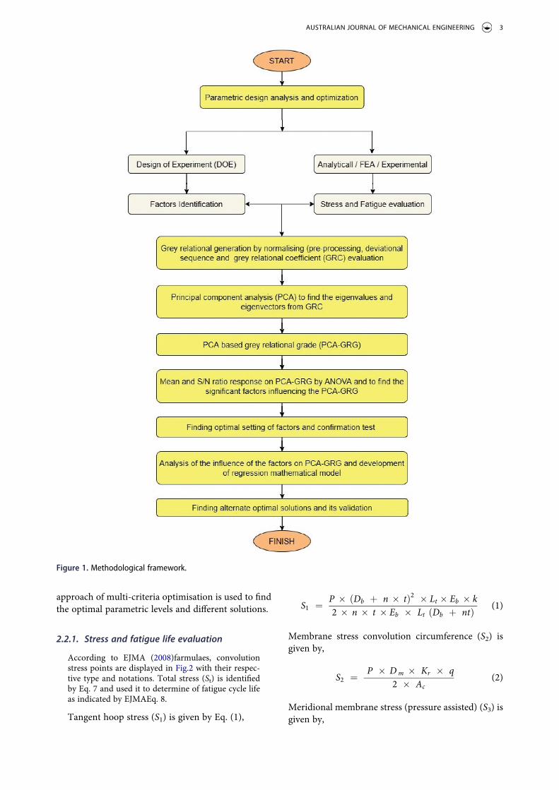
approach of multi-criteria optimisation is used to find the optimal parametric levels and different solutions.

2.2.1. Stress and fatigue life evaluation

According to EJMA (2008)farmulaes, convolution stress points are displayed in Fig.2 with their respec-tive type and notations. Total stress (St) is identified by Eq. 7 and used it to determine of fatigue cycle life as indicated by EJMAEq. 8.

Tangent hoop stress (S1) is given by Eq. (1),

S1 ¼P � Db þ n � tð Þ

2� Lt � Eb � k

2 � n � t � Eb � Lt Db þ ntð Þ(1)

Membrane stress convolution circumference (S2) is given by,

S2 ¼P � D m � Kr � q

2 � Ac(2)

Meridional membrane stress (pressure assisted) (S3) is given by,

Figure 1. Methodological framework.

AUSTRALIAN JOURNAL OF MECHANICAL ENGINEERING 3

S3 ¼P � H

2 � n � tp(3)

Meridional bending stress (pressure-assisted) (S4) is given by,

S4 ¼P

2 nHt p

� � 2

� Cp (4)

Meridional membrane stress (displacement-assisted) (S5) is given by,

S5 ¼E � t 2 � d p � λ � θ0

4 � H 3 � C f � N � sin λ2

� � (5)

Meridional bending stress (displacement-assisted) (S6) is given by,

S6 ¼5 � E � tp � dp� λ � θ0

6 � H 2 � N � C d sin λ2

� � (6)

Total stress component (St) is given by EJMA as,

St ¼ 0:7 � ðS3 þ S4Þ þ ðS5 þ S6Þ (7)

Allowable number of fatigue cycles are calculated by,(7)

Nf ¼Ko

Kg � Ea=Eb

� �St � Sa

(8)

The meanings of the symbols and notations used in the preceding equations are described in the nomen-clature section. Figure 2 depicts the stress locations on the bellows convolution surface. The root of the convolution is extended to the tangent section of the bellows, which is the source of S1 stress. The S2 stress is induced to the flat annular plate that connects the top and lower toroidal halves of the convolution. The tangent and circumferential membrane stress are

calculated using Eqs. (1) and (2), respectively. The crown toroidal section is susceptible to meridional membrane (S3) and meridional bending (S4) type stresses due to the pressured internal fluid. These stresses can be calculated analytically using Eqs. (3) and (4). The effect of convolution deflection is dis-placement at the root of the convolution, which is most often owing to the thermal effect or pressurised fluid. As illustrated in Figure 2, the stress generated at the root of the convolution is generally the deflec-tion base membrane and bending stresses (S5 and S6), which can be calculated using Eqs.(5) and (6), respec-tively. EJMA provides two helpful equations for cal-culating stress-based fatigue cycles: Eq. (7) and Eq. (8). FEA analysis is used to verify the fatigue cycles for the specific design configuration of the bellows.

The bellows geometrical model is symmetrical in terms of its longitudinal central axis. The load applied to the bellows and placing the boundary conditions is in fact, even symmetric. For the finite element model-ling of the bellows, the axisymmetric element type Plane-183 is adopted. The convolution openings at the root and crown sections radially move when pres-sure is applied to the bellows. As a result, the half convolution portion resembles a curved beam with fixed ends and no axial motion as shown in Figure 2 (b). However, additional half of the axial displacement is taken into account, which is distributed proportion-ally across all convolutions. As illustrated in Figure 2 (b), the displacement boundary condition is applied at the top nodes.

To verify the results of the stress analysis by EJMA, the experimental set-up was developed as shown in Figure 3 with the supporting fixtures, air compressor (to supply the pressurised air) and four-channel strain indicator. The foil type electrical resistance strain

Figure 2. (a) Stress measurement locations on convolution and symbols for the type of stresses. (b) End conditions on the section of the convolution.

4 N. D. PAGAR

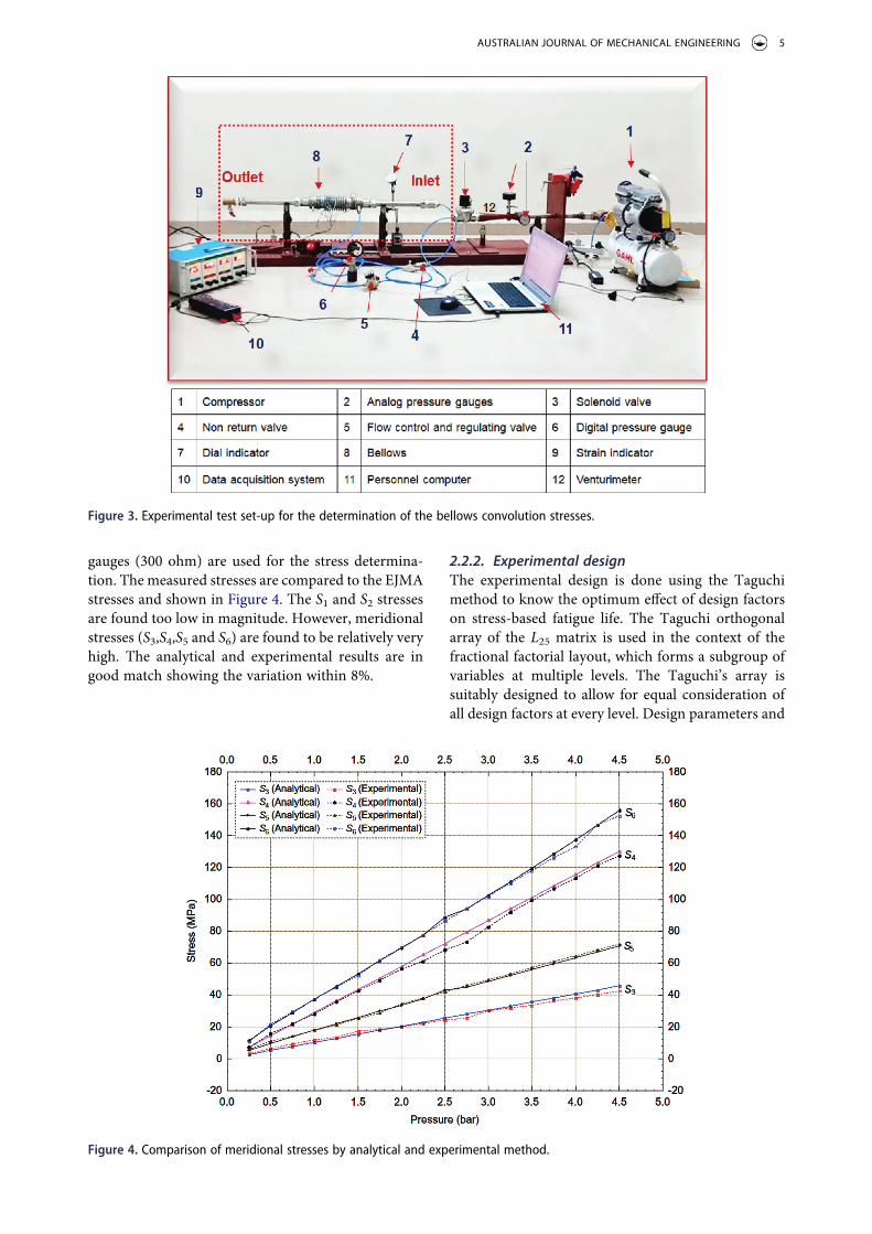
gauges (300 ohm) are used for the stress determina-tion. The measured stresses are compared to the EJMA stresses and shown in Figure 4. The S1 and S2 stresses are found too low in magnitude. However, meridional stresses (S3,S4,S5 and S6) are found to be relatively very high. The analytical and experimental results are in good match showing the variation within 8%.

2.2.2. Experimental designThe experimental design is done using the Taguchi method to know the optimum effect of design factors on stress-based fatigue life. The Taguchi orthogonal array of the L25 matrix is used in the context of the fractional factorial layout, which forms a subgroup of variables at multiple levels. The Taguchi’s array is suitably designed to allow for equal consideration of all design factors at every level. Design parameters and

Figure 3. Experimental test set-up for the determination of the bellows convolution stresses.

Figure 4. Comparison of meridional stresses by analytical and experimental method.

AUSTRALIAN JOURNAL OF MECHANICAL ENGINEERING 5

levels used in this work are listed in Table 1. It consists of five design geometric factors of bellows. The mini-misation of the maximum induced stresses and max-imisation of the fatigue cycle life is the function of these design factors. The objective function used in the multi-response optimisation process is given in the Eq. 9.

f ðNc;H; q; tp;DpÞ ¼ Min MaxðS1; S2; S3; S4; S5; S6f g and Max fNf g

(9)

The constraints used for the design specifications are stated in Eq.10. All these constraints are based on the design limits imposed by EJMA. According to it, con-volution stress generation depends on the geometrical configuration and topology.

The Taguchi method is a statistical technique used in the Design of Experiments (DOE) by various researchers, which exists amongst the different system designs as a single response optimisation. It effectively reduces the experimental trials needed to achieve opti-mal response functions compared to the full factorial DOE. Taguchi orthogonal array matrix has been required to be implemented in the design process using a general fractional factorial design. In this work, the orthogonal array matrix used is L25(54) for constructing the 25 experimental runs and shown in Table 2 with evaluation of different convolution stres-ses and life cycles, for each experimental run. The design parameters used in the Taguchi technique are not so sensitive to control the variabilities in unma-nageable situations and other noise influencing para-meters (Wu 2002, Pagar N.D. et al., 2020b).

As a consequence, the loss function is measured in terms of the differences occurred between the experi-mental output and the expected output, and it is reformed into the signal-to-noise (S/N) ratio. Further, S/N ratio is being treated as a base for the optimality selection, where its higher values are the representatives of the improved quality index of per-formance factors. Depending on the objective func-tion, the following are the S/N ratio defining approaches used in conventional DOE and stated in the form of the logarithmic functions of the responses, as shown by the Eq.11, Eq.12, and Eq.13.

4 � Nc � 12

6 � H � 18

4 � q � 12

0:3 � tp � 0:7

40 � Dp � 200 (10)

(1) Lower-the better (LTB)

SN

� �

LTB¼ � 10 � log10

1n

Xn

i¼ 1y2

i

" #

(11)

(1) Normal-the better (NTB)

SN

� �

NTB¼ 10 � log 10

�y2

s2

� �

(12)

(1) Higher-the better (HTB)

SN

� �

HTB¼ � 10 � log10

1n

Xn

i¼1

1y2

i

" #

(13)

In the above equations, yi and n indicate the response for the ith orthogonal run and the number of the experimental run, respectively. Also, yi

2 and s2 present the mean responses and variance of the collected data, respectively. If the objective function is considered for the minimisation of the responses, then LTB is pre-ferred. For maximisation and target values, HTB and NTB approaches are implemented, respectively. Stress evaluation results for each Taguchi experimental run are shown in Table 2.

2.2.3. Methodology of GRA computationsGrey relational analysis method is a comprehensive tool to overcome the uncertainties and complexities in discrete or continuous parametric data. In multiple responses, if the effect and relationship between qual-ity performance attributes are ambiguous or distinct, it is referred to as ‘grey’, indicating poor or uncertain data. In this method, multiple responses are translated into the equivalent single representative grade referred to as the grey relational grade (GRG). Following is the procedure of finding of GRG (Sylajakumari, Ramkrishnasamy, and Palaniappan 2018).

Step 1: Normalisation of the dataThe initial stage of GRA is preprocessing of the

original information of responses presented in the data, which need to be transformed in the normal-ised form. At this stage, the initial reference and comparability sequence are transferred into a non- dimensional form and data between values ranging from 0 to 1 can be viewed. The original reference sequence (x0) of j entities is given as,

x0 ¼ x0ð1Þ; x0ð2Þ . . . . . . . . . ; x0ðjÞ; . . . . . . ::x0ðnÞ½ �

(14)

Similarly, the comparative sequence of j entities is given as,

Table 1. Design parameters and level.

Parametrs Notation

Level Unit1 2 3 4 5

Number of convolutions NC 4 6 8 10 12Convolution height H 6 9 12 15 18 mmConvolution Pitch q 4 6 8 10 12 mmPly thickness tp 0.3 0.4 0.5 0.6 0.7 mmPitch diameter Dp 40 80 120 160 200 mm

6 N. D. PAGAR

xi ¼ xið1Þ; xið2Þ . . . . . . . . . ; xiðjÞ; . . . . . . ::xiðnÞ½ � (15)

Depending on the goal of optimisation, whether to maximise or minimise or between certain specific target values, the transformed form of the reference and comparative sequences have three types. As fol-lows, it is described:

(1) Larger-the-best case: This is used for the max-imisation problems. Translation from xiðjÞto xi�ðjÞ is given as normalised comparative form,

xi�ðjÞ ¼

xiðjÞ � Min½xiðjÞ�Max½xiðjÞ� � Min½xiðjÞ�

(16)

(1) Nominal-the-best case: This is used for the specific target values xobðjÞ problems.

xi�ðjÞ ¼

xiðjÞ � xobðjÞj j

Max½xiðjÞ� � xobðjÞ(17)

(1) Smaller-the-best case: This is used for the mini-misation problems.

xi�ðjÞ ¼

Max½xiðjÞ� � xiðjÞMax½xiðjÞ� � Min½xiðjÞ�

(18)

At the same time, conversion of the normalised refer-ence sequence is represented as,

x�O ¼ x�oð1Þ; x�oð2Þ . . . . . . . . . ; x�oðjÞ; . . . . . . ::x�oðnÞ

� �

(19)

Step 2: Deviational sequence (ΔoiðjÞ)The expression used to get the deviational sequence

is given by,

Table 2. Parametric design levels, convolution stresses, total stress and number of cycles.

Run

Design levels Convolution stresses (MPa) Total stress Number of cyclesNc H q tp Dp S1 S2 S3 S4 S5 S6 (St) (Nf)

1 4 6 4 0 40 0.5 0.9 3.8 11.1 3.8 12.126.3

7.48 × 105

2 4 9 6 0 80 0.7 1.0 4.2 14.2 5.8 14.733.4

8.59 × 104

3 4 12 8 1 120 0.8 1.0 4.5 16.2 7.8 16.538.8

9.61 × 104

4 4 15 10 1 160 0.9 1.1 4.7 17.6 9.8 17.743.2

1.05 × 105

5 4 18 12 1 200 1.0 1.1 4.8 18.7 11.7 18.746.9

1.15 × 105

6 6 6 6 1 160 1.1 0.8 2.3 3.6 7.2 8.519.8

9.63 × 104

7 6 9 8 1 200 1.1 0.9 2.8 5.9 9.9 11.827.8

7.69 × 104

8 6 12 10 1 40 0.2 1.0 3.2 6.6 15.0 16.238.0

9.45 × 104

9 6 15 12 0 80 0.9 2.7 9.4 48.9 34.8 140.0215.7

1.19 × 105

10 6 18 4 0 120 1.0 0.7 8.4 70.8 3.5 34.593.5

5.62 × 105

11 8 6 8 1 80 0.4 0.7 1.6 1.6 11.9 7.521.7

6.86 × 104

12 8 9 10 0 120 1.4 2.2 5.6 20.1 30.5 68.3116.8

6.63 × 105

13 8 12 12 0 160 1.4 1.9 5.6 21.2 32.7 65.7117.2

6.79 × 105

14 8 15 4 1 200 1.4 0.5 5.6 30.3 3.8 20.649.6

1.22 × 105

15 8 18 6 1 40 0.2 0.7 5.6 28.3 8.8 46.478.8

2.95 × 105

16 10 6 10 0 200 1.7 1.6 2.8 4.8 31.8 32.869.9

2.16 × 105

17 10 9 12 1 40 0.3 1.7 3.4 6.0 40.9 29.076.5

2.71 × 105

18 10 12 4 1 80 0.5 0.4 3.8 13.4 4.3 15.932.2

8.39 × 104

19 10 15 6 1 120 0.6 0.6 4.0 14.9 7.5 21.041.7

1.02 × 105

20 10 18 8 0 160 1.8 1.7 11.2 109.4 22.7 296.3403.5

1.13 × 105

21 12 6 12 1 120 0.7 1.3 1.9 2.0 37.5 20.460.6

1.63 × 105

22 12 9 4 1 160 0.8 0.4 2.4 4.7 4.5 8.818.3

6.45 × 104

23 12 12 6 0 200 2.3 1.3 7.5 49.4 16.0 106.4162.3

9.08 × 105

24 12 15 8 0 40 0.3 1.4 7.0 31.6 28.6 384.8440.5

8.77 × 103

25 12 18 10 1 80 0.5 1.3 6.8 34.1 30.1 152.9211.6

1.31 × 105

AUSTRALIAN JOURNAL OF MECHANICAL ENGINEERING 7

ΔoiðjÞ ¼ x�oðjÞ � x�i ðjÞ��

�� (20)

It is the difference between the normalised reference and comparable sequences at jth point.

Step 3: Grey relational coefficient (�)For the GRC computation, the equation is used as,

�iðjÞ ¼Δmin þ ΨΔmax

ΔoiðjÞ þ ΨΔmax(21)

The above expression depends on the Δmin and Δmax, the differences between the lowest and highest values of each responsive variable. The distinguished coeffi-cient is shown by Ψ and in the ranges of Ψ 2 ð0; 1Þ. In common, empiricallyΨ is chosen as 0.5 to distribute the equally weighted values to every responses.

Step 4: Grey relational grade (γ) computationsIt is found by adding the grey relationship coeffi-

cients, as shown in Eq.21. The GRG of ith experimental run has been specified by ‘γi’ as well as the ‘n’ denotes the number of attributed variables. GRG indicates the quality attributes of the response variables and its values range from 0 to 1. The multiple responses associated with problems are then converted into a single-grade entity.

GRGðγiÞ ¼1n

Xn

j¼1�iðjÞ (22)

A good relationship between the design parameter settings at the specific level is established and antici-pated as optimal by the higher range values of the determined GRG. Besides that, the effect of each para-meter on the outcome of the process is not always the same in the case of practical applications. Previous researchers prefer to use the same weight attributes to the responses, which in the different attributed characteristics prevents heterogeneity. The traditional way of assessing the allocated variables of each quality attribute relies heavily on prior knowledge and the mechanism of trial error, resulting in uncertainty dur-ing the decision-making phase of optimisation. Therefore, to demonstrate the comparable weight values of the output response characteristics of the variables in the GRA, principal components (PC) are added (Sutono et al. 2017; Raissi 2020a). The PCA is used to assign all quality response attributes to the exact weights. So, Eq.22 has been updated in Eq.23.

PCA � GRGðγiÞ ¼1n

Xn

j¼1ωj � �iðjÞ� �

(23)

In the above Eq. 23,ωj shows the weighted value of variable j. The weighting value ωj can be derived from the PCA and it is implemented to assign the weight values to every attributed variable of the GRC. The principal components are combined with the GRC and the weights of every responsive attributed variable are computed. This implies that the GRC multiplies

the related performance attribute variables by weight factors (eigenvalues obtained from the eigenvector of the related PC). GRG indicates the degree of the effect of the comparable sequence that exerted on the refer-ence sequences and also correlated the optimality of the response variables.

2.2.4. Principal component analysis (PCA)The PCA describes the structure of variance and cov-ariance of each performance parameter by sequentially integrating it to all. The process includes the essential stages as given below:

Step 1Normalised performance factors are utilised to for-

mulate the matrix form of the variance and covariance (Ki), and it is shown in the Eq. 24,

KiðjÞ, i = 1 to m, j = 1 to n

KiðjÞ ¼

K1ð1Þ K1ð2Þ . . . K1ðnÞK2ð1Þ...

K2ð2Þ . . .

..

.K2ðnÞ...

Kmð1Þ Kmð2Þ KmðnÞ

0

BB@

1

CCA (24)

For the above matrix form, m indicates the number of experimental runs conducted in the optimisation pro-cess, and n implies the number of quality attributes considered. Here, K reflects the grey relational coeffi-cient of each quality characteristic. In this case, the total number of performance attributes is all convolu-tion stress responses, n ¼ 6 and orthogonal run, m ¼ 25.

Step 2The matrix representing the correlational coeffi-

cient is determined by the use of Eq. 25 as follows:

Rjl ¼covðKiðjÞ;KiðlÞσKiðjÞ � σKiðlÞ

� �

(25)

In the above equation, KiðjÞ and KiðlÞ indicate the response sequences to which covariance are calculated for j = 1 to n and l = 1 to n.

σKiðjÞ and σKiðlÞ show the standard deviations (S. D.) for the response sequences KiðjÞ and KiðlÞ, respectively.

Step 3Principal components are directly found out from

the eigenvalues and higher values are preferred to find the multiplication factor. Eigenvectors are computed by the use of the correlation coefficients and presented in the matrix form. The following equation shows the relation of it.

ðR � λkImÞVik ¼ 0 (26)

In the above Eq. 26, λk is characterised by the eigen-values, and the term Vik refers to the respective eigenvectors.

8 N. D. PAGAR

Xn

k¼1T

λk ¼ n and Vik ¼ ½ak1ak2 . . . . . . ::akn� (27)

Here, K varies from the 1 to n inStep 4The expression for determining the principal com-

ponents is shown by Eq. 28,

ymk ¼Xn

iXmðiÞ � Vik (28)

In the above equation, ym1shows the first principal component as well as ym2 shows the second principal component.

2.2.5. Analysis of variance (ANOVA) for optimalityGrey relational grade is further used in the ANOVA analysis to find the most significant factors influencing the responses. It is done by removing the complete variance in the PCA-GRG, which contains a number of squared deviations of the mean PCA-GRG added by all factors and error. The ANOVA table is commonly used to assess the correlations between factors and the influence of these relations on the dependent variables or responses. The contribution (in percentage) of each input parameter to the total sum of the squared devia-tions can be used to quantify the abrupt change in response characteristics. Normally, the Fisher-F ratio is widely used as a metric to assess the magnitude of the effect of the test results and is often referred to as the F-test. The p-value indicates the probability of significance from the graph at 95% of the confidence limit and, if it is less than 0.05, the relative factor is considered to be a significant factor. In addition, the corresponding F-value (Fisher’s ratio) can also be observed and its highest value shows significance. Most importantly, ANOVA table signifies two values; one is a correlational coefficient (R2) and other is adjusted correlational coefficient (R2

adj) and their higher values show the excellent fitment of the ANOVA model. It analyses the variable quantity referred to input factors and their relationship, which primarily affects the characteristics of the responses. The ANOVA table is widely used to evaluate the interactions between variables and their effect on the response variable. The optimal setting of the factors can be obtained from the mean PCA-GRG or S/N response map. It is the highest maximum PCA-GRG for the corresponding values of the quality attributes. From the mean PCA-GRG or S/N response map, the optimal setting of the factors can be obtained. For all the corresponding values of quality attributes, it is the highest maximum PCA-GRG (Pradhan 2013).

2.2.6. Confirmation test and regression analysisIf the optimal configuration of the design specifica-tions has been determined by ANOVA, the confirma-tion test shall be carried out. It could record the

accuracy of the overall performance attributes of the PCA-GRG and the expected responses. Estimation of the predicted grey relational grade ( η^ ) of the opti-mum parametric selection is given by,

η^ ¼ ηmþXb

i¼1ðηi � ηmÞ (29)

In the case of realistic systems, the designer’s view of deciding the choice of optimum design variables, which includes uncertainty in terms of availability, reliability, expense, time and working conditions. In order to fix this issue, the designer needs suitable alternative solutions with close resemblance to the desired optimal design parameters. In order to achieve this, the regression model ought to be designed in such a way that it demonstrates the overall response beha-viour to predict various alternative optimal solutions. The manufacturer or supplier may reduce the risk of taking decisions that would waste their resources. In particular, it is important to note that the PCA-GRG approach is being used in this current research to optimise discrete-independent geometric parameters at the design stage itself (Ni 2012).

3. Results and discussion

3.1. Behaviour of stress-based fatigue life for different bellows configurations

As illustrated in Table 2, the Taguchi orthogonal array (L25) depicts the 25 bellows configurations. For each run, Eq. 7 is used to compute the total stress (St), and the Eq. 8 is used to compute the allowable number of fatigue cycles (Nf). The evaluation of the meridional stresses (S3toS6) is carried out by using the Eqs. (3–6). The behaviour of the fatigue cycles (Nf ) in relation to the meridional stresses of pressure type and deflection type (S3,S4,S5,S6) and total stress (St) is shown in Figure 5 for each L25 Taguchi run. From Figure 5, it is revealed that for the identical bellows configuration (of any Taguchi run), the meridional stress magnitude for each corresponding stress type is different, demon-strating distinct fatigue cycles. For instance, 23rd run shows the higher life cycles at approximately 7 MPa of S3, 50 MPa for S4, 15 MPa for S5 and 85 MPa for S6. The similar observations can be seen in Figure 5 for the other run. As a result, selecting the design config-uration that minimises stresses while maximising fati-gue life is difficult. The multi-criteria optimisation technique (simultaneous optimisation) is used with PCA-GRG to obtain optimal designs. The determina-tion of the principal component-based grey relational grade is described in Sections 2.1.3 and 2.1.4. The objective function is a blend of stress reduction (S3, S4, S5, S6 and St) and maximisation of fatigue life (Nf), as stated by Eq. 9.

AUSTRALIAN JOURNAL OF MECHANICAL ENGINEERING 9

3.2. Determination of the PCA based grey relational grade (PCA-GRG)

3.2.1. Normalisation (Pre-processing)For all Taguchi L25 run of the design matrix, meridio-nal stresses (S3toS6), total stress (St) and fatigue cycles (Nf) are transformed in the non-dimensional form. It uses the larger-the-best approach to maximise fatigue life (Nf) and given by Eq. 16. The smaller-the-best approach is used to minimise the stresses and given by Eq. 18. Sample calculation for the 1st experimental run to calculate the normalised form is given as:

S3 ¼11:250� 3:75011:250� 1:607 ¼ 0:778 S4 ¼

109:369� 11:143109:369� 1:640 ¼ 0:912 S5 ¼

40:935� 3:80140:935� 2:001 ¼ 0:954

S6 ¼384:815� 12:096384:504� 2:093 ¼ 0:974 St ¼

440:504� 26:322440:504� 6:725 ¼ 0:955 Nf ¼

908335� 74801908335� 8776 ¼ 0:073

3.2.2. Deviational sequence (Δoi)The deviational sequence between the normalised and comparable reference data of all response attributes is calculated by Eq. 20.The maximum deviational sequence (Δmax) is 1.00, and the minimum deviational sequence (Δmin) is zero. Sample calculation for the 1st

experimental run is given as follows: Δo1ðS3Þ ¼ 1:000 � 0:778j j ¼ 0:222;-Δo1ðS4Þ ¼ 1:000 � 0:954j j ¼ 0:088 Δo1ðS5Þ ¼ 1:000 � 0:954j j ¼ 0:046;-Δo1ðS6Þ ¼ 1:000 � 0:974j j ¼ 0:026 Δo1ðStÞ ¼ 1:000 � 0:955j j ¼ 0:045;Δo1ðNf Þ ¼ 1:000 � 0:073j j ¼ 0:927

3.2.3. To find grey relational coefficient (�)After calculating the deviational sequence, the grey relational coefficient (GRC) is computed by Eq. 21. This equation depends on the difference between the lowest and highest values of each response attribute.

The sample calculation of grey relational coefficient (GRC) for the 1st experimental run is given as follows: �ðS3Þ ¼

0:00þ0:5�1:000:222þ0:5�1:00 ¼ 0:692�ðS4Þ ¼

0:00þ0:5�1:000:088þ0:5�1:00 ¼ 0:850-

�ðS5Þ ¼0:039þ0:5�1:000:046þ0:5�1:00 ¼ 0:987�ðS6Þ ¼

0:014þ0:5�1:000:026þ0:5�1:00 ¼ 0:977-

�ðStÞ ¼0:00þ0:5�1:00

0:045þ0:5�1:00 ¼ 0:963�ðNf Þ ¼0:00þ0:5�1:00

0:927þ0:5�1:00 ¼ 0:350

3.2.4. Principal component-based GRC (PCA-GRC)Principal components are found from the eigenvalues using Eq. 26 and Eq. 28 and presented in Table 3. Scree-plot is shown in Figure 6, which depicts the contribution of the eigenvalue to the corresponding PC. The eigenvalue for the first PC is 3.764, and the second PC is 1.158, which contributes 62.7% and 19.3%, respectively. The proportions of the first two PCs are added to find the eigenvectors showing weight values, as displayed in Table 4. In the next step, these weight factors are multiplied to the GRC for finding the principal component-based GRG, as shown in Table 5. Sample calculation for the 1st Taguchi run is given as follows: � S3½ �PCA ¼ 0:692� ð0:0338Þ ¼ 0:023 � S4½ �PCA ¼ 0:850� ð0:0122Þ ¼ 0:010 � S5½ �PCA ¼ 0:985� ð0:4187Þ ¼ 0:4124 � S4½ �PCA ¼ 0:976� ð0:2748Þ ¼ 0:268 � St½ �PCA ¼ 0:963� ð0:2825Þ ¼ 0:272 � Nf½ �PCA ¼ 0:350� ð� 0:022Þ ¼ � 0:008

Figure 5. Behaviour of the number of fatigue cycles and stresses (S3, S4, S5, S6, and St) for each specified Taguchi L25 orthogonal experimental run.

Table 3. Eigenvalue analysis of the correlation matrix for principal components (PC) used in the simultaneous optimisa-tion of meridional stress and fatigue life cycles.

Variables

Principal components (PC)

PC-1 PC-2 PC-3 PC-4 PC-5 PC-6

Eigenvalue 3.7642 1.1587 0.883 0.1445 0.0446 0.0051Proportion 0.627 0.193 0.147 0.024 0.007 0.001Cumulative 0.627 0.82 0.968 0.992 0.999 1.000

10 N. D. PAGAR

3.2.5. Computation of the PCA-GRG for simultaneous optimisation of stress-based fatigue lifeIn order to calculate the PCA-GRG by applying the Eq. 23, the PCA-dependent grey relational coefficient is used. The proportional weight is allocated by the PCA to all response attributes. In Table 6, the com-puted PCA-GRG is presented with rank. For the Taguchi experimental run to be utilised, the rank indicates the priority of the optimal responses. The strong correlation between the comparable sequence

Figure 6. Screeplot for the eigenvalue of principal component (PC) in simultaneous optimisation of stress based fatigue.

Table 4. Weight contribution factors assigned to respective simultaneous responses (stress and life cycles) computed from the eigenvectors of the respective principal components.

Stress responses

Principal components (PC) Weight factorPC-1 PC-2 PC-3 PC-4 PC-5 PC-6

S3 0.454 −0.371 −0.099 0.532 −0.603 0.026 0.0338S4 0.449 −0.419 −0.115 0.148 0.736 −0.217 0.0122S5 0.261 0.766 0.166 0.516 0.147 −0.174 0.4187S6 0.481 0.193 −0.193 −0.577 −0.258 −0.543 0.2748St 0.497 0.196 −0.115 −0.26 0.077 0.792 0.2825Nf −0.214 0.16 −0.948 0.167 0.043 0.007 −0.0220

Table 5. Principal component-based grey relational coefficient (PCA-GRC) of the simultaneous optimisation of the total stress and cycle life.

Run

PCA-GRC

PCA-GRGS3 S4 S5 S6 St Nf

1 0.023 0.010 0.412 0.268 0.272 −0.008 0.1412 0.022 0.010 0.373 0.265 0.264 −0.008 0.1323 0.021 0.010 0.341 0.262 0.257 −0.008 0.1254 0.021 0.009 0.314 0.261 0.253 −0.008 0.1195 0.020 0.009 0.291 0.259 0.249 −0.008 0.1146 0.030 0.012 0.349 0.273 0.280 −0.008 0.1317 0.027 0.011 0.313 0.269 0.270 −0.008 0.1228 0.025 0.011 0.260 0.263 0.258 −0.008 0.1109 0.013 0.006 0.157 0.161 0.146 −0.008 0.06610 0.014 0.005 0.419 0.240 0.208 −0.012 0.13311 0.034 0.012 0.289 0.275 0.278 −0.008 0.12012 0.018 0.009 0.171 0.208 0.193 −0.014 0.07913 0.018 0.009 0.164 0.210 0.192 −0.015 0.07714 0.018 0.008 0.413 0.257 0.246 −0.008 0.13815 0.018 0.008 0.327 0.228 0.220 −0.009 0.11416 0.027 0.012 0.167 0.242 0.227 −0.009 0.08817 0.025 0.011 0.140 0.247 0.221 −0.009 0.08318 0.023 0.010 0.402 0.263 0.265 −0.008 0.13819 0.023 0.010 0.345 0.256 0.254 −0.008 0.12520 0.011 0.004 0.206 0.109 0.100 −0.007 0.06521 0.032 0.012 0.149 0.257 0.235 −0.008 0.08822 0.029 0.012 0.398 0.273 0.283 −0.008 0.14123 0.015 0.006 0.251 0.180 0.168 −0.022 0.08624 0.016 0.008 0.179 0.092 0.094 −0.007 0.05725 0.016 0.008 0.173 0.155 0.147 −0.008 0.069

Table 6. Table showing the number of cycles (Nf) by analytical and FEA method, PCA-GRG and improvement in PCA-GRG, S/N ratio and rank.

Run

Number of cycles(Nf) PCA- GRG

S/N ratio Rank

Improvement in PCA-GRGAnalytical FEA

1 7.48 × 105 7.58 × 104 0.141 −16.99 1 0.0342 8.59 × 104 8.47 × 104 0.132 −17.56 6 0.0953 9.61 × 104 9.53 × 104 0.125 −18.05 9 0.1454 1.05 × 105 1.09 × 105 0.119 −18.47 12 0.1855 1.15 × 105 1.19 × 105 0.114 −18.83 14 0.2196 9.63 × 104 9.51 × 104 0.131 −17.63 7 0.1037 7.69 × 104 7.94 × 104 0.122 −18.25 10 0.1648 9.45 × 104 9.26 × 104 0.110 −19.15 15 0.2479 1.19 × 105 1.23 × 105 0.066 −23.62 23 0.55010 5.62 × 105 5.51 × 105 0.133 −17.51 5 0.09011 6.86 × 104 6.55 × 104 0.120 −18.38 11 0.17712 6.63 × 105 6.59 × 105 0.079 −22.10 20 0.46413 6.79 × 105 6.87 × 105 0.077 −22.24 21 0.47214 1.22 × 105 1.25 × 105 0.138 −17.22 4 0.05915 2.95 × 105 3.03 × 105 0.114 −18.83 13 0.21816 2.16 × 105 2.26 × 105 0.088 −21.13 17 0.40017 2.71 × 105 2.83 × 105 0.083 −21.66 19 0.43518 8.39 × 104 8.16 × 104 0.138 −17.19 3 0.05619 1.02 × 105 9.62 × 104 0.125 −18.04 8 0.14420 1.13 × 105 1.18 × 105 0.065 −23.79 24 0.55921 1.63 × 105 1.49 × 105 0.088 −21.07 16 0.39622 6.45 × 104 6.68 × 104 0.141 −17.03 2 0.03923 9.08 × 105 9.37 × 105 0.086 −21.29 18 0.41124 8.77 × 103 8.85 × 103 0.057 −24.83 25 0.60825 1.31 × 105 1.21 × 105 0.069 −23.25 22 0.530

Average overall improvement in PCA-GRG (for all Taguchi run) = 0.2719 (27.19%)

AUSTRALIAN JOURNAL OF MECHANICAL ENGINEERING 11

and the reference sequence indicates a higher PCA- GRG value. For the first Taguchi run, the sample calculation is shown as follows:

γiðPCA � GRGÞ ¼1n

Xn

j¼1½ωj � �ðjÞ�

¼16½0:0233þ 0:0103þ 0:4124þ 0:2682

þ0:2720 � 0:089� ¼ 0:141

3.3. Stress-based fatigue life of bellows by FEA analysis

The fatigue life of the bellows is evaluated using FEA analysis with ANSYS 16.0 software for each configura-tion associated with the L25 Taguchi run. Table 6

shows the number of fatigue cycles computed using FEA. Figure 7 shows the graphical representation of fatigue life cycle evaluated by analytical method and FEA, for each Taguchi run from 1 to 25. The mini-mum number of cycles found by FEA is 8.85 × 103 for 24th Taguchi run and maximum number of cycles are found by FEA is 9.37 × 105 cycles for 23rd run. From Figure 7, it shows that total stress (St) for 23rd run is 162.3 MPa and that for 24th run is 440.5 MPa. Figure 7 depicts simplified details of design alternatives that can provide a longer life cycle in the stress cycle range of 100 MPa to 200 MPa. This will assist the designer in making better setup choices. A sample example of cycle life determination by ANSYS 16.0 is shown in Figure 8 for the 4th Taguchi run. It shows the fatigue life of 1:091� 105cycles.

Figure 7. Behaviour of the number of fatigue cycles and total stress (St) or the each specified Taguchi L25 orthogonal experimental run computed by analytical and FEA method.

Figure 8. Number of fatigue life cycles determined by FEA for the 4th Taguchi experimental run of four convolution bellows (Nc

= 4).

12 N. D. PAGAR

3.4. ANOVA to determine the optimality of stress-based fatigue life by PCA-GRG

ANOVA is performed using PCA-GRG to determine the optimal design parameters. The mean PCA-GRG response table for the simultaneous optimisation of total stress and fatigue life for each level of design parameters is shown in Table 7. The optimum value is specified by the higher PCA-GRG of the design parametric level. For all design parameters, the higher mean PCA-GRG values are 0.126, 0.113, 0.128, 0.122 and 0.110, respectively, at levels that are optimal. The mean PCA-GRG is 0.1125. The main effect plot of the PCA-GRG of the stress-based fatigue life is shown in Figure 9, and the optimal parameter settings are found as Nc � 1; H � 1; q � 1; tp � 5; Dp � 3. Higher PCA-GRG values indicate a reduction in stress and

optimised life of the respective design configuration of bellows. Rank defines the priorities of the fac-tors asq>Nc > tp >H >Dp.

With the help of ANOVA, the effect of the signifi-cant design parameters on PCA-GRG is assessed. The Fisher’s-F ratio and the probability of significance (p-value) are found from the ANOVA computations and shown in Table 8 by S/N ratios of PCA-GRG, at 95% of confidence limit.

From the ANOVA table of the S/N ratio of PCA- GRG, R2 is 99.26% and R2(adj) is 95.55%, which indi-cates the aptness of the statistical model. For deter-mining the S/N ratio, ‘Larger-the-better’ approach is chosen for PCA-GRG. The contribution (%) of Nc, q and tpis found as 23.26%, 43.31% and 24.68%, respectively. The p-value of the Nc, q and tpis found as 0.003, 0.001 and 0.003, respectively, which indicates that these factors are the most significant factors. The contribution (%) of H and Dp is 5.67% and 2.34%, respectively. The p-value of the Hand Dp is found as 0.037 and 0.146, respectively. Therefore, from S/N ratio of PCA-GRG, the most influencing design para-meters are the Nc, q and tp.

After determining the optimal design parametric level, the last step of the PCA-based grey relation analysis is to confirm the predicted PCA-GRG with experimental PCA-GRG. Prediction of PCA-GRG is

Table 7. Mean response table for the PCA-GRG of simulta-neous optimisation of total stress and fatigue life.

Factors

Levels Delta (Max-Min) Rank1 2 3 4 5

Nc 0.126 0.112 0.105 0.099 0.088 0.0382 2H 0.113 0.111 0.107 0.101 0.099 0.0148 4q 0.128 0.117 0.098 0.097 0.085 0.0525 1tp 0.087 0.097 0.109 0.116 0.122 0.0349 3Dp 0.106 0.105 0.110 0.106 0.109 0.0089 5

Total mean grey relational grade = 0.1125

Figure 9. Main effect of PCA-GRG of simultaneous optimisation of the stress responses and fatigue life cycles on design parameters, namely, Nc, H, q, tp, and Dp.

Table 8. Analysis of variance for the mean S-N ratios of PCA-GRG (simultaneous optimisation of total stress and fatigue life).Source DF Seq SS Adj SS Adj MS F P Contribution (%) Remark

Nc 4 34.093 34.093 8.523 31.330 0.003 23.26 Most significantH 4 8.314 8.314 2.078 7.640 0.037 5.67 Less significantq 4 63.489 63.489 15.872 58.340 0.001 43.31 Most significanttp 4 36.179 36.179 9.045 33.240 0.003 24.68 Most significantDp 4 3.423 3.423 0.856 3.150 0.146 2.34 InsignificantResidual Error 4 1.088 1.088 0.2721Total 24 146.587 146.587 R2 = 99.26%R2 (adj) = 95.55%

AUSTRALIAN JOURNAL OF MECHANICAL ENGINEERING 13

calculated by using Eq. 29 and it is obtained as 0.1519. The calculation is shown as follows:

η^ ¼ ηmþXq

i¼1ðηi � ηmÞ

¼ 0:1125þ 0:1265 � 0:1125ð Þ

þ 0:1282 � 0:1125ð Þ þ ð0:1222 � 0:1125Þ¼ 0:1519

For the optimal parametric setting given by ANOVA, experimental PCA-GRG is 0.1463 and shown in Table 9. Predicted and experimental values are very close to each other. The average overall improvement in PCA- GRG for all L25 Taguchi run is 27.19%.

(1) Determination of an alternate optimal solution using a mathematical regression model of PCA- GRG for simultaneous optimisation.

Using PCA-GRG, a regression model is established by taking the 95% confidence limit. It gives a correlation coefficient values as R2 ¼ 98:18% and expression for the mathematical model (multiple regression) is stated in Eq. 30, as given below:

PCA � GRG ¼ 0:2119 �0:00657 � Nc � 0:001151 � H þ 0:02034� q þ 0:09395 � tp þ 0:000059 � Dp

þ 0:000734 � q2 � 0:000263 ðNc � qÞ(30)

The higher value of the R2indicates the suitability of the model fitment. The different alternative optimal solution is given by the multiple regression model and the design parametric levels are shown in Table 10.

As indicated in Table 10, the alternative optimal solu-tion provides a set of design parameters as well as opti-mised life cycles for each solution with lower stress values. Experimental PCA-GRG results are obtained for

alternate optimal solutions. Alternative optimal solutions for PCA-GRG are verified using regression and Taguchi prediction techniques, and the results are compared to the experimental PCA-GRG and shown in Table 11. The findings are quite similar to each other, as can be seen in the graphical depiction presented in Figure 10. Variation in the PCA-GRG results by an experimental run and regression prediction is observed from 0.48% to 4.49%, and the absolute average deviation is 2.53%. In addition, the variation in the PCA-GRG results by an experimental run and Taguchi prediction is observed from 4.2% to 8.31% and the absolute average deviation is 4.93%.

In this analysis, it is found that the minimisation of the meridional stress factor (St) assists to optimise the fatigue life cycles and provides the suitable design configuration of the bellows. It is also seen that the life cycles deter-mined for the alternate optimal solution as well as from L25 Taguchi run has been found in the range of 1.133 × 105 cycles to the 9.083 × 105 cycles. This shows that range of fatigue life cycles of the bellows found in the low cycle, finite fatigue regime.

4. Conclusions

This manuscript exhibits the new approach to the hand-ling of discrete parametric design of convoluted bellows to enhance the stress-based fatigue life. Multifaceted con-volution stresses show the different life cycles; hence, simultaneous optimisation method proves the applicabil-ity to predict the stress-based fatigue life. The minimisa-tion of the meridional stress factor (St) assists to optimise the fatigue life cycles and provides the suitable selection of bellows design configuration. ANOVA and multiple regression models are used to get the number of optimal solutions of design parametric levels. The experimental PCA-GRG found is 0.146 and the predicted PCA-GRG is 0.151, which is verified by confirmation test. The most influencing design parameters are the Nc, q and tp. It is

Table 9. Confirmation test for PCA-GRG of simultaneous optimisation.

Response

Optimal parametric design setting

Predicted Experimental

Optimal parametric settings Nc −1, H-1, q-1, tp −5, Dp −3

PCA-GRG 0.1519 0.1463Average overall improvement in PCA-GRG (For all Taguchi run) 27.19%

Table 10. Stress responses and number of optimised cycles obtained for the alternate optimal design level using multiple regression model of PCA-GRG of simultaneous optimisation.

Alternate solution

Design parametric levels Stress responses and number of optimised cycles

NC H q tp Dp S3 S4 S5 S6 St Nf

1 4 6 4 0.7 200 1.62 12.45 3.81 13.41 27.06 7.59 × 104

2 4 6 4 0.7 120 1.60 14.82 5.76 16.20 33.45 8.60 × 104

3 4 6 4 0.3 40 3.75 16.05 7.81 16.09 37.76 9.41 × 104

4 12 9 4 0.7 160 2.41 17.65 9.87 19.29 43.20 1.06 × 105

5 8 15 4 0.5 200 5.63 23.07 11.94 20.26 52.29 1.31 × 105

6 6 6 6 0.5 160 2.25 3.61 7.24 8.47 19.82 6.64 × 104

7 10 12 4 0.6 80 3.75 7.54 10.11 12.23 30.25 8.07 × 104

14 N. D. PAGAR

seen that the life cycles determined for the alternate optimal solution as well as L25Taguchi run found in the range from 1.133 x 105cycles to the 9.083 × 105 cycles. It demonstrates the spectrum of fatigue life in the low-cycle, finite fatigue regime of the bellows material. This work helps designer to understand the complex interactions between the factors and responses in early design stage and simplify the decision-making. Therefore, the designer can select the suitable configuration of the bel-lows at initial stage with the reduced convolution stresses and optimised fatigue cycles.

Disclosure statement

No potential conflict of interest was reported by the author(s).

Notes on contributor

Dr. Nitin D. Pagar has obtained his Bachelor’s in Mechanical Engineering from Government College of Engineering, Aurangabad, Master’s in Design Engineering from Pune University and obtained PhD from in

Mechanical and Materials Technology from the Department of Technology, SPPU, Pune. He has about 15 years of Teaching Experience and 4 years of Research / Industrial experience. His area of interest includes Structural Dynamics, Multi- Attributed Decision Making (MADM) Parametric Optimization, Stress Analysis, Materials and Design. Recently, he is working as a Teaching Faculty at MIT School of Engineering (Mechanical Department), MIT-ADT University, Pune. He is Permanent member of ISTE and Indian Institute of Metals (IIM). Author also working as a reviewer of many International peer-reviewed indexed international journals and conferences.

Data availability statement:

The author confirm that the data supporting the findings of this study are available within the article. Any other data if necessary could be available by corresponding author on reasonable request.

Nomenclature

SaAmbient permissible stressηmAverage of grade relational gradesλ Coefficient for the characteristics equationAcCross-sectional area bellowsKoFatigue factor considering the material and manufac-

turing constant (forKg factor less than 448 MPa)KgFatigue strength reduction constant = 0.5ηiHighest values of the average GRG of the relevant sig-

nificant optimal parameterEbModulus of ElasticityEaModulus of elasticity of bellows at ambient

temperatureEbModulus of elasticity of bellows at design temperature

x�i Normalised comparative sequencex�oNormalised referential sequence

nNumber of pliesbNumber of significant parameters resulting from the

ANOVA tableLtTangent length of bellowstpThickness of convolution (total)

Table 11. Comparison between experimental PCA-GRG and predicted PCA-GRG of simultaneous optimisation of the total stress and fatigue life cycles (by multiple regression and Taguchi prediction model).

Sr. No. Optimal settingsExperimental PCA-

GRG

Predicted PCA-GRG

By regression

By Taguchi

1 Nc-1 H-1 q-1tp-5 Dp-5

0.142 0.143 0.164

2 Nc-1 H-1 q-1tp-5 Dp-3

0.134 0.147 0.165

3 Nc-1 H-1 q-1tp-1 Dp-1

0.126 0.137 0.140

4 Nc-5 H-2 q-1tp-5 Dp-4

0.120 0.138 0.141

5 Nc-3 H-4 q-1tp-3 Dp-5

0.113 0.136 0.137

6 Nc-2 H-1 q-2tp-3 Dp-4

0.131 0.131 0.134

7 Nc-4 H-3 q-1 tp-4 Dp-2

0.121 0.133 0.140

Figure 10. Comparison of the PCA-GRG (simultaneous optimisation of stress and fatigue life) of the predicted alternate optimal run determined by the experimental, regression and Taguchi method.

AUSTRALIAN JOURNAL OF MECHANICAL ENGINEERING 15

DbTotal diameter of bellows

References

Becht, C. IV. 2002. “An Evaluation of EJMA Stress Calculations for Unreinforced Bellows, Journal of Pressure Vessel Technology.” Transactions of The ASME,124, 124-129.

EJMA. 2008. Standards of Expansion Joint Manufacturers Association. 9th ed. New- York.

Hao, Z. L., C. Y. Xi, Z. H. Huang, C. H. Zhang, and J.T Jun Ting Luo. 2018. “Hydraulic Bulging Process with Axial Feedings and Strain Field of U-shaped Metal Bellows.” Journal of Central South University 25 (11): 2712–2721. doi:10.1007/s11771-018-3948-8.

Hong, Y. Y., H. M. Hsieh, and S. Y. Ho. 2007. “Determination of Locations for Static Transfer Switches Using Genetic Algorithms and Fuzzy Multi-objective Programming. International.” Journal of Electrical Power & Energy Systems 29 (6): 480–487. doi:10.1016/j.ijepes.2006.11.007.

Kaushik, N., and S Singhal. 2018. “Hybrid Combination of Taguchi-GRA-PCA for Optimization of Wear Behavior in AA6063/SiCp Matrix Composite.” Production & Manufacturing Research 6 (1): 171–189. doi:10.1080/ 21693277.2018.1479666.

Ko, B.G., G.J. Park, and W.I. Lee. 1995. “Mechanical Behavior of U –shaped Bellows and Shape Optimal Design Using Multiple Objective Optimization Method.” KSME Journal 9, 91-101.

Li, Y. 1990. “Strength Analysis and Structural Optimization of U-shaped Bellows.” International Journal of Pressure Vessels and Piping 42 (1): 33–46. doi:10.1016/0308- 0161(90)90053-K.

Liu, J., H. Li, Y. Liu, L Li, and C. Sun. 2018. “Size Effect Related Hydroforming Characteristics of Thin-walled 316-L Bellows considering Pressure Change. The.” International Journal of Advanced Manufacturing Technology 98 (1–4): 505–522. doi:10.1007/s00170-018-2280-7.

Mahajan, K.A., and R. Pawade. 2021.“Effect of Machining Parameters and Vibration on Polymethylmethacrylate Curved Surface in Single-point Diamond Turning.” Journal of Micromanufacturing 4(1), 74-83.

Mehat, N. M., S. Kamaruddin, A.R. Othman, N.M. Mehat, and S Kamaruddin. 2014. “Hybrid Integration of Taguchi Parametric Design, Grey Relational Analysis, and Principal Component Analysis Optimization for Plastic Gear Production.” Chinese Journal of Engineering 351206 (1–11): 2014.

Naveen Kumar, J. P., J. S. Kumar, R.K. SarathiJeyathilak, M. Venkatesh, A. S. Christopher, and K. C. Ganesh. 2017. “Effect of Design Parameters on the Static Mechanical Behaviour of Metal Bellows Using Design of Experiment and Finite Element Analysis.” International Journal on Interactive Design and Manufacturing (Ijidem) 11 (3): 535–545. doi:10.1007/s12008-016-0306-7.

Nemeth, B., A. Molnar, S. Bozoki, K. Wijaya, A. Inotai, J. D Campbell, and Z Kalo. 2019. “Comparison of Weighting Methods Used in Multi-criteria Decision Analysis Frameworks in Healthcare with Focus on Low and Middle Income Countries.” Journal of Comparative Effectiveness Research 8 (4): 195–204. doi:10.2217/cer-2018- 0102.

Ni, C. C. 2012. “Grey Relational Grade Analysis between Vickers Hardness and Fatigue Crack Growth Data of 2024-T351 Aluminum Alloy.” Advanced Materials

Research 476: 2435–2439. www.scientific.net/AMR.476- 478.2435

Pagar, N. D, and H. Gawande. 2020a. “Parametric Design Analysis of Meridional Deflection Stresses in Metal Expansion Bellows Using Gray Relational Grade.” J Braz. Soc. Mech. Sci. Eng 42 (256): 2020. doi:10.1007/ s40430-020-02327-0.

Pagar, N. D., and H. Gawande. 2020b. “Multi-response Design Optimisation of Convolution Stresses of Metal Bellows Using Integrated PCA-GRA Approach.” Australian Journal of Mechanical Engineering 1–21. (Published online). doi:10.1080/14484846.2020.1725347.

Panda, A., A.K. Sahoo, and R. Rout. 2016. “Multi-attribute Decision Making Parametric Optimization and Modeling in Hard Turning Using Ceramic Insert through Grey Relational Analysis: A Case Study.” Decision Science Letters 5 (4): 581–592. doi:10.5267/j.dsl.2016.3.001.

Pradhan, M. K. 2013. “Estimating the Effect of Process Parameters on MRR, TWR and Radial Overcut of EDMed AISI D2 Tool Steel by RSM and GRA Coupled with PCA.” International Journal of Advanced Manufacturing Technology 68 (1–4): 591–605. doi:10.1007/s00170-013-4780-9.

Raissi, H. 2020a. “Stress Analysis in Adhesive Layers of a Five-layer Circular Sandwich Plate Subjected to Temperature Gradient Based on Layerwise Theory.” In Mechanics of Advanced Materials and Structures. (Published online, 2020)

Raissi, H., M. Shishehsaz, and S Moradi. 2019. “Stress Distribution in a Five-layer Sandwich Plate with FG Face Sheets Using Layerwise Method.” Mechanics of Advanced Materials and Structures 26 (14): 1234–1244. doi:10.1080/15376494.2018.1432796.

Raissi, H., M. Shishesaz, and S. Moradi. 2017. “Applications of Higher Order Shear Deformation Theories on Stress Distribution in a Five Layer Sandwich Plate.” Journal of Computational Applied Mechanics 48 (2): 233–252.

Safari, M., J. Joudaki, and Y Ghadiri. 2019. “A Comprehensive Study of the Hydroforming Process of Metallic Bellows: Investigation and Multi-objective Optimization of the Process Parameters.” International Journal of Engineering 32 (11): 1681–1688.

Shishehsaz, M., H. Raissi, and S Moradi. 2020. “Stress Distribution in a Five-layer Circular Sandwich Composite Plate Based on the Third and Hyperbolic Shear Deformation Theories.” Mechanics of Advanced Materials and Structures 27 (11): 927–940. doi:10.1080/ 15376494.2018.1502379.

Sutono, S.B., H.A. Salwa, Z. Taha, and Subagyo. 2017. “Integration of Grey-based Taguchi Method and Principal Component Analysis for Multi-response Decision-making in Kansei Engineering.” European Journal of Industrial Engineering 11 (2): 205–228. doi:10.1504/EJIE.2017.083254.

Sylajakumari, P. A., R. Ramkrishnasamy, and G Palaniappan. 2018. “Taguchi Grey Relational Analysis for Multi Response Optimization of Wear in Co-continuous Composite.” Materials 11 (1743): 1–17.

Velasquez, M., and P. T. Hester. 2013. “An Analysis of Multi-criteria Decision Making Methods.” International Journal of Operations Research 10 (2): 56–66.

Wu, H. 2002. “A Comparative Study of Using Grey Relational Analysis in Multiple Attribute Decision Making Problems.” Quality Engineering 15 (2): 209–217. doi:10.1081/QEN-120015853.

16 N. D. PAGAR