MARINE ECOLOGY PROGRESS SERIESMar Ecol Prog Ser

Vol. 335: 207–216, 2007 Published April 16

INTRODUCTION

Successful management of cetacean populationsrequires information on their foraging habitats (Bjørge2002). Therefore, a growing number of studies quan-tify relationships between habitat use and basic envi-ronmental features in order to generate predictionmodels of marine mammal distribution (e.g. Gregr &Trites 2001, Hamazaki 2002). Model predictors areoften chosen based on their availability, althoughchoice of variables should rather derive from ecologi-

cal theory (Gregr 2004). Common predictors ofcetacean distribution include sea surface temperature(SST), distance to shore, and underwater topography(e.g. Hoelzel et al. 1989, Woodley & Gaskin 1996) butthe mechanisms linking these variables to patterns ofhabitat selection have begun to be investigated onlyrecently (e.g. Croll et al. 2005). Nevertheless, identify-ing cause–effect relationships in ecological models iscritical (Hilborn & Mengel 1997).

The distribution of rorqual whales on their feedinggrounds is mostly related to the abundance and patch-

© Inter-Research 2007 · www.int-res.com*Email: thomas.doniol-valcroze@mail.mcgill.ca

Influence of thermal fronts on habitat selection by four rorqual whale species in the Gulf of St. Lawrence

Thomas Doniol-Valcroze1, 2, 3,*, Dominique Berteaux3, Pierre Larouche4, Richard Sears2

1Department of Natural Resource Sciences, McGill University, 21111 Lakeshore Road, Ste.-Anne-de-Bellevue, Quebec H9X 3V9, Canada

2Mingan Island Cetacean Study, 285 Green, St. Lambert, Quebec J4P 1T3, Canada3Canada Research Chair in Conservation of Northern Ecosystems and Centre d’etudes nordiques,

Université du Québec à Rimouski, 300 allée des Ursulines, Rimouski, Quebec G5L 3A1, Canada4Institut Maurice-Lamontagne, 850 route de la Mer, PO Box 1000, Mont-Joli, Quebec G5H 3Z4, Canada

ABSTRACT: Understanding the factors influencing habitat selection is critical to improving manage-ment and conservation plans for large whales. Many studies have linked the distribution of cetaceansto basic environmental features such as underwater topography and sea surface temperature (SST),but the mechanisms underlying these relationships are poorly understood. Dynamic mesoscale pro-cesses like thermal fronts are prime candidates to link physiographic factors to whale distributionbecause they increase biological productivity and aggregate prey. However, previous studies of largewhales have found little evidence of such associations, possibly because they were not at the appro-priate spatio-temporal scales. We quantified the relationship between SST fronts and the distributionof blue Balaenoptera musculus, finback B. physalus, humpback Megaptera novaeangliae and minkeB. acutorostrata whales in the northern Gulf of St. Lawrence. We compared the distribution of 1094whale sightings collected from boat surveys conducted in 1996 to 2000 to the locations of frontal areasdetermined from 61 satellite maps. The distributions of whales and thermal fronts were highly corre-lated (random resampling and Mantel tests of matrix similarity). Spatial distributions differed amongspecies, probably reflecting differences in feeding strategies. Identification of surface fronts fromsatellite imagery thus effectively complemented field observations of whales. These findings signifi-cantly increase our understanding of habitat quality in rorqual whales, and encourage a greater useof dynamic environmental variables in future studies of whale habitat use.

KEY WORDS: Sea surface temperature · Thermal fronts · Blue whale · Finback whale · Humpbackwhale · Minke whale · Habitat selection · Gulf of St. Lawrence

Resale or republication not permitted without written consent of the publisher

Mar Ecol Prog Ser 335: 207–216, 2007

iness of krill (Murase et al. 2002) and fishes (White-head & Carscadden 1985). Patchiness of organisms incoastal ecosystems is often caused by the dynamicfeatures of mesoscale oceanographic processes likefronts, eddies and upwellings (Olson & Backus 1985).These processes usually involve spatial scales of 1 to10 km and temporal scales of 1 to 10 d (Hofmann &Powell 1998). In most cases, when these upwellingsreach the surface, one of their manifestations is a ther-mal gradient between warm surface waters and coldupwelled waters. Such mesoscale oceanographic pro-cesses increase biological productivity and aggregateprey species (Olson & Backus 1985), thus influencingthe distribution of several pelagic fish species (e.g.Fiedler & Bernard 1987, Podesta et al. 1993).

Gaskin (1987) predicted that these transition zonesbetween tidally mixed and thermally stratified areascould be an important feature of right whale habitat inthe lower Bay of Fundy. This hypothesis was supportedby some anecdotal evidence (Murison & Gaskin 1989)but not by quantitative results (Woodley & Gaskin1996). Similarly, Baumgartner et al. (2003) suggestedthat spatial and interannual variability in right whaleoccurrence on the Scotian shelf may be associated withSST gradients, but Baumgartner & Mate (2005) foundno evidence that tagged right whales associated withsuch fronts. Several cetacean species do concentratenear mesoscale features and coastal upwelling areas(e.g. Monterey Bay, Benson et al. 2002; Gulf of Mexico,Davis et al. 2002) but specific information on rorqualwhales is very scarce. Hamazaki (2002) showed thatrorqual abundance was related to areas with highermonthly probability of front occurrence but this rela-tionship was never investigated spatially, nor at a finertime-scale.

Long-term studies of rorqual whales in the northernGulf of St. Lawrence (Quebec, Canada) have shownthat distribution of blue Balaenoptera musculus, fin-back B. physalus, humpback Megaptera novaeangliaeand minke B. acutorostrata whales is linked to areas ofheterogeneous sea-bottom topography (T. Doniol-Valcroze & R. Sears unpubl. data). Naud et al. (2003)found a similar relationship for minke whales studiedin a subset of the same research area, and thereforethis link appears strong across several spatial scales(1 to 10 km grid cells). However, these studies alsoshowed significant variation in time that could not beexplained by static bathymetric factors. Satelliteremote sensing shows that surface temperature in theSt. Lawrence is strongly influenced by tidal mixing andupwellings and can vary quickly (Thibault et al. 2002).Such mesoscale processes could provide additionalexplanation for the temporal variability observed inwhale habitat use. Because these upwellings can beinduced by local changes in sea-bottom topography

(Hui 1985, Marchand et al. 1999), the resulting thermalfronts might constitute an important link betweenphysiographic factors and whale distribution patterns.

Here we consider the influence of a dynamic oceano-graphic feature on habitat selection of rorqual whalesthrough the use of biological (whale sightings) andphysical (satellite-derived SST) data collected at finespatial and temporal scales. We test the hypothesis thatspatio-temporal distribution of 4 species of rorqualwhales in the northern Gulf of St. Lawrence is relatedto thermal fronts. More specifically, we predict thatwhales should be found closer to SST fronts thanexpected under a random scenario, and that between-species differences should reflect species-specificfeeding strategies.

MATERIALS AND METHODS

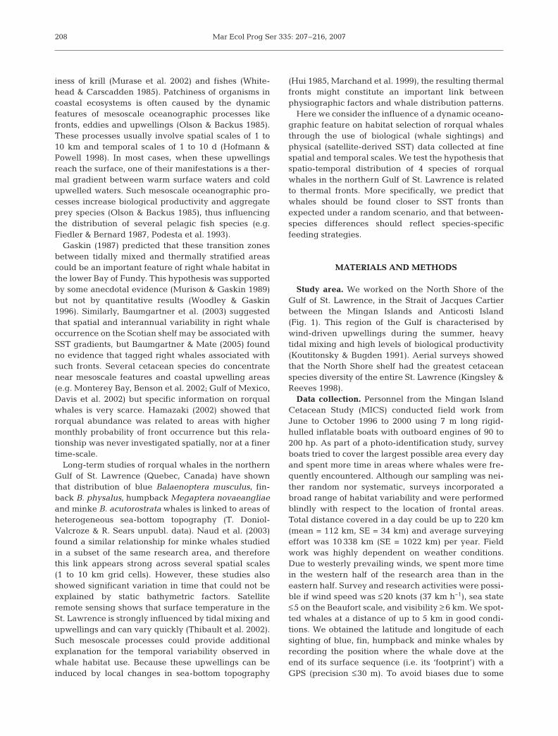
Study area. We worked on the North Shore of theGulf of St. Lawrence, in the Strait of Jacques Cartierbetween the Mingan Islands and Anticosti Island(Fig. 1). This region of the Gulf is characterised bywind-driven upwellings during the summer, heavytidal mixing and high levels of biological productivity(Koutitonsky & Bugden 1991). Aerial surveys showedthat the North Shore shelf had the greatest cetaceanspecies diversity of the entire St. Lawrence (Kingsley &Reeves 1998).

Data collection. Personnel from the Mingan IslandCetacean Study (MICS) conducted field work fromJune to October 1996 to 2000 using 7 m long rigid-hulled inflatable boats with outboard engines of 90 to200 hp. As part of a photo-identification study, surveyboats tried to cover the largest possible area every dayand spent more time in areas where whales were fre-quently encountered. Although our sampling was nei-ther random nor systematic, surveys incorporated abroad range of habitat variability and were performedblindly with respect to the location of frontal areas.Total distance covered in a day could be up to 220 km(mean = 112 km, SE = 34 km) and average surveyingeffort was 10 338 km (SE = 1022 km) per year. Fieldwork was highly dependent on weather conditions.Due to westerly prevailing winds, we spent more timein the western half of the research area than in theeastern half. Survey and research activities were possi-ble if wind speed was ≤ 20 knots (37 km h–1), sea state≤ 5 on the Beaufort scale, and visibility ≥ 6 km. We spot-ted whales at a distance of up to 5 km in good condi-tions. We obtained the latitude and longitude of eachsighting of blue, fin, humpback and minke whales byrecording the position where the whale dove at theend of its surface sequence (i.e. its ‘footprint’) with aGPS (precision ≤ 30 m). To avoid biases due to some

208

Doniol-Valcroze et al.: Influence of thermal fronts on whales

individuals being sighted several times in the sameobservation day, we used photo-identification tech-niques to retain only the first sighting of each individ-ual in the analysis.

Satellite data were received from the National Oceanicand Atmospheric Administration (NOAA), processed bythe Remote Sensing Laboratory of the Maurice Lamon-tagne Institute and then published using the St.Lawrence Observatory web site (www. osl.gc.ca). Rawdata received each day from the ‘advanced very highresolution radiometer’ (AVHRR) were transformed intoSST maps covering the entire Gulf of St. Lawrence usingTerascan™ software. Images were geo-referenced auto-matically using coastline recognition. Temperatureswere calculated using a split-window algorithm (Mc-Clain et al. 1985).

Data mapping and identification of thermal fronts.For our analysis, we used data obtained on days forwhich a good quality satellite map of SST was avail-able (with no clouds masking the study area) and forwhich weather conditions permitted field surveys. Foreach of these observation days, a GIS coverage wasbuilt by plotting the sightings on a map projected inUniversal Transverse Mercator with a central meridianof –63° longitude, using ArcView 3.1 software with the‘spatial analyst’ and the ‘animal movement’ extensions(Hooge & Eichenlaub 1997). Satellite images of SSTwere incorporated into the GIS as raster (cell-based)layers. Pixels measured 1.132 km and were calibratedto temperature values in intervals of 0.256°C. Frontsare usually defined as ‘narrow regions where hori-zontal gradients are large’ (Mann & Lazier 1991) but

definitions vary with respect to the strength of the gra-dient. For Ullman & Cornillon (1999), each front re-presented a change in SST >0.375°C km–1. In contrast,Marchand et al. (1999) observed fronts in the Estuaryof the St. Lawrence with typical temperature gradientsof 2 to 5°C over a few kilometres. We identified tem-perature gradients on each SST map by applying aLaplace filter to a series of circular matrices of 3 pixelsin diameter. The centre pixel of each matrix returneddata on the range of temperature values across thatmatrix. This edge-detection filter can identify fronts inany direction. Preliminary analysis showed that theaverage temperature gradient in our data set was0.58°C km–1 (SD = 0.65). Gradients of 1.88°C km–1 thusrepresented 2 standard deviations above the mean.Based on this, we decided to define SST fronts asgradients of 2°C km–1, which represented only thestrongest temperature gradients.

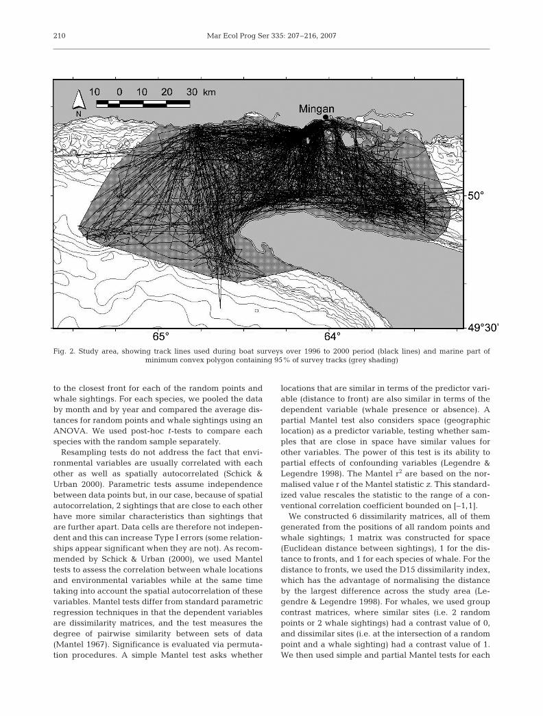
Statistical analyses. We used a random resamplingapproach (Manly et al. 2002) to test the null hypothesisthat whale sightings were distributed randomly withrespect to thermal fronts. For each year, we drew theminimum convex polygon (MCP) containing 95% ofour effort tracks. We used a land mask to remove theshape of the landmasses and created a buffer of 500 maround the shorelines to ensure that the polygon rep-resented available habitat for whales (Fig. 2). For eachobservation day, we plotted random points within theMCP representing the study area of that year, in equalnumber to whale sightings. This ensured that randompoints fell in areas that were well covered by our sur-vey effort. We then calculated the Euclidean distance

209

Fig. 1. Atlantic coast of Canada showing location of study area and main bathymetric contours

Mar Ecol Prog Ser 335: 207–216, 2007

to the closest front for each of the random points andwhale sightings. For each species, we pooled the databy month and by year and compared the average dis-tances for random points and whale sightings using anANOVA. We used post-hoc t-tests to compare eachspecies with the random sample separately.

Resampling tests do not address the fact that envi-ronmental variables are usually correlated with eachother as well as spatially autocorrelated (Schick &Urban 2000). Parametric tests assume independencebetween data points but, in our case, because of spatialautocorrelation, 2 sightings that are close to each otherhave more similar characteristics than sightings thatare further apart. Data cells are therefore not indepen-dent and this can increase Type I errors (some relation-ships appear significant when they are not). As recom-mended by Schick & Urban (2000), we used Manteltests to assess the correlation between whale locationsand environmental variables while at the same timetaking into account the spatial autocorrelation of thesevariables. Mantel tests differ from standard parametricregression techniques in that the dependent variablesare dissimilarity matrices, and the test measures thedegree of pairwise similarity between sets of data(Mantel 1967). Significance is evaluated via permuta-tion procedures. A simple Mantel test asks whether

locations that are similar in terms of the predictor vari-able (distance to front) are also similar in terms of thedependent variable (whale presence or absence). Apartial Mantel test also considers space (geographiclocation) as a predictor variable, testing whether sam-ples that are close in space have similar values forother variables. The power of this test is its ability topartial effects of confounding variables (Legendre &Legendre 1998). The Mantel r2 are based on the nor-malised value r of the Mantel statistic z. This standard-ized value rescales the statistic to the range of a con-ventional correlation coefficient bounded on [–1,1].

We constructed 6 dissimilarity matrices, all of themgenerated from the positions of all random points andwhale sightings; 1 matrix was constructed for space(Euclidean distance between sightings), 1 for the dis-tance to fronts, and 1 for each species of whale. For thedistance to fronts, we used the D15 dissimilarity index,which has the advantage of normalising the distanceby the largest difference across the study area (Le-gendre & Legendre 1998). For whales, we used groupcontrast matrices, where similar sites (i.e. 2 randompoints or 2 whale sightings) had a contrast value of 0,and dissimilar sites (i.e. at the intersection of a randompoint and a whale sighting) had a contrast value of 1.We then used simple and partial Mantel tests for each

210

Fig. 2. Study area, showing track lines used during boat surveys over 1996 to 2000 period (black lines) and marine part of minimum convex polygon containing 95% of survey tracks (grey shading)

Doniol-Valcroze et al.: Influence of thermal fronts on whales

combination of these matrices, using 10 000 iterationsto assess significance. We performed analyses usingthe R package for multivariate and spatial analysis,Version 4.0 (Casgrain & Legendre 2001).

RESULTS

Observation days and whale sightings

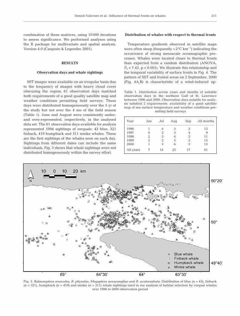
SST images were available on an irregular basis dueto the frequency of images with heavy cloud coverobscuring the region; 61 observation days matchedboth requirements of a good quality satellite map andweather conditions permitting field surveys. Thesedays were distributed homogeneously over the 5 yr ofthe study but not over the 4 mo of the field season(Table 1). June and August were consistently under-and over-represented, respectively, in the analyseddata set. The 61 observation days available for analysisrepresented 1094 sightings of rorquals: 43 blue, 321finback, 419 humpback and 311 minke whales. Theseare the first sightings of the whales seen on each day.Sightings from different dates can include the sameindividuals. Fig. 3 shows that whale sightings were notdistributed homogeneously within the survey effort.

Distribution of whales with respect to thermal fronts

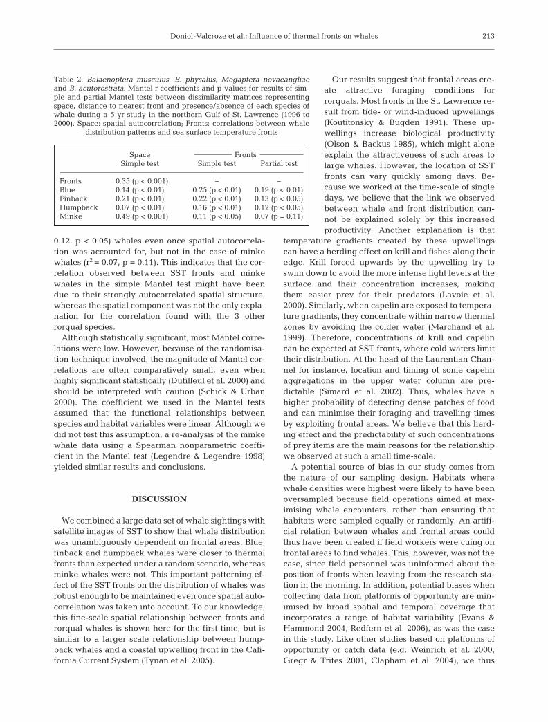
Temperature gradients observed in satellite mapswere often steep (frequently >2°C km–1) indicating theoccurrence of strong mesoscale oceanographic pro-cesses. Whales were located closer to thermal frontsthan expected from a random distribution (ANOVA,F4 = 7.45, p < 0.001). We illustrate this relationship andthe temporal variability of surface fronts in Fig. 4. Thepattern of SST and frontal areas on 2 September, 2000(Fig. 4A,B) is characteristic of a wind-induced up-

211

Table 1. Distribution across years and months of suitableobservation days in the northern Gulf of St. Lawrencebetween 1996 and 2000. Observation days suitable for analy-sis satisfied 2 requirements: availability of a good satellitemap of sea surface temperature and weather conditions per-

mitting field surveys

Year Jun Jul Aug Sep All months

1996 1 4 5 3 131997 0 2 3 4 91998 2 3 4 2 111999 3 2 5 5 152000 1 3 6 3 13

All years 7 14 23 17 61

Fig. 3. Balaenoptera musculus, B. physalus, Megaptera novaeangliae and B. acutorostrata. Distribution of blue (n = 43), finback(n = 321), humpback (n = 419) and minke (n = 311) whale sightings used in our analysis of habitat selection by rorqual whales

over 1996 to 2000 observation period

Mar Ecol Prog Ser 335: 207–216, 2007

welling with fronts lying in a general east–west axis.The configuration on 23 August, 2000 (Fig. 4C,D)shows the typical result of tidal forces with discontinu-ous irregular fronts, some of them in a north–southaxis. Post-hoc t-tests showed that the relationship be-tween whales and thermal fronts was not the same forall species: the difference between whale sightingsand random points was statistically significant for blue(t84 = 8.41, p < 0.001), finback (t640 = 5.91, p < 0.001) andhumpback (t836 = 6.87, p < 0.001), whales but margin-ally non-significant for minke whales (t620 = 1.79, p =0.08). On average, blue whales were the closest to thefronts, followed by humpback, finback, minke whalesand random points. This order remained remarkablystable over the 4 mo of the study (Fig. 5), except in Julywhen finback whales were found slightly closer to thefrontal areas than humpback whales. Each species wasfarther away from the fronts in June than in any othermonth, which was also true of the random points.

Simple Mantel tests between space and the othermatrices showed strong spatial autocorrelations for allspecies of whales as well as for the SST fronts(Table 2). Simple Mantel tests also showed significantcorrelations between the SST front matrix and all 4whale matrices, confirming the results of the resam-

pling test: points that were similar in terms of whalepresence were also similar in their distance to thefrontal areas. A partial Mantel test showed that therewas a significant effect of the distribution of SST frontson distribution of blue (Mantel partial r2 = 0.19, p <0.01), finback (r2 = 0.13, p < 0.05) and humpback (r2 =

212

Fig. 4. Sea surface temperature (SST), location of frontal areas, whale sightings (d), random points (s) and shortest straight lineslinking sightings or random points to the closest thermal front. (A) SST map dated 2 September 2000 and (B) associated SST frontstypical of upwellings induced by westerly winds; (C) SST map dated 23 August 2000 and (D) associated SST fronts typical

of tidally induced upwellings. Specific names as in Fig. 3 legend

Fig. 5. Balaenoptera musculus, B. physalus, Megaptera no-vaeangliae and B. acutorostrata. Mean (±SE) distancesbetween whale sightings or random points and the nearest

frontal area for years 1996 to 2000

Doniol-Valcroze et al.: Influence of thermal fronts on whales

0.12, p < 0.05) whales even once spatial autocorrela-tion was accounted for, but not in the case of minkewhales (r2 = 0.07, p = 0.11). This indicates that the cor-relation observed between SST fronts and minkewhales in the simple Mantel test might have beendue to their strongly autocorrelated spatial structure,whereas the spatial component was not the only expla-nation for the correlation found with the 3 otherrorqual species.

Although statistically significant, most Mantel corre-lations were low. However, because of the randomisa-tion technique involved, the magnitude of Mantel cor-relations are often comparatively small, even whenhighly significant statistically (Dutilleul et al. 2000) andshould be interpreted with caution (Schick & Urban2000). The coefficient we used in the Mantel testsassumed that the functional relationships betweenspecies and habitat variables were linear. Although wedid not test this assumption, a re-analysis of the minkewhale data using a Spearman nonparametric coeffi-cient in the Mantel test (Legendre & Legendre 1998)yielded similar results and conclusions.

DISCUSSION

We combined a large data set of whale sightings withsatellite images of SST to show that whale distributionwas unambiguously dependent on frontal areas. Blue,finback and humpback whales were closer to thermalfronts than expected under a random scenario, whereasminke whales were not. This important patterning ef-fect of the SST fronts on the distribution of whales wasrobust enough to be maintained even once spatial auto-correlation was taken into account. To our knowledge,this fine-scale spatial relationship between fronts androrqual whales is shown here for the first time, but issimilar to a larger scale relationship between hump-back whales and a coastal upwelling front in the Cali-fornia Current System (Tynan et al. 2005).

Our results suggest that frontal areas cre-ate attractive foraging conditions forrorquals. Most fronts in the St. Lawrence re-sult from tide- or wind-induced upwellings(Koutitonsky & Bugden 1991). These up-wellings increase biological productivity(Olson & Backus 1985), which might aloneexplain the attractiveness of such areas tolarge whales. However, the location of SSTfronts can vary quickly among days. Be-cause we worked at the time-scale of singledays, we believe that the link we observedbetween whale and front distribution can-not be explained solely by this increasedproductivity. Another explanation is that

temperature gradients created by these upwellingscan have a herding effect on krill and fishes along theiredge. Krill forced upwards by the upwelling try toswim down to avoid the more intense light levels at thesurface and their concentration increases, makingthem easier prey for their predators (Lavoie et al.2000). Similarly, when capelin are exposed to tempera-ture gradients, they concentrate within narrow thermalzones by avoiding the colder water (Marchand et al.1999). Therefore, concentrations of krill and capelincan be expected at SST fronts, where cold waters limittheir distribution. At the head of the Laurentian Chan-nel for instance, location and timing of some capelinaggregations in the upper water column are pre-dictable (Simard et al. 2002). Thus, whales have ahigher probability of detecting dense patches of foodand can minimise their foraging and travelling timesby exploiting frontal areas. We believe that this herd-ing effect and the predictability of such concentrationsof prey items are the main reasons for the relationshipwe observed at such a small time-scale.

A potential source of bias in our study comes fromthe nature of our sampling design. Habitats wherewhale densities were highest were likely to have beenoversampled because field operations aimed at max-imising whale encounters, rather than ensuring thathabitats were sampled equally or randomly. An artifi-cial relation between whales and frontal areas couldthus have been created if field workers were cuing onfrontal areas to find whales. This, however, was not thecase, since field personnel was uninformed about theposition of fronts when leaving from the research sta-tion in the morning. In addition, potential biases whencollecting data from platforms of opportunity are min-imised by broad spatial and temporal coverage thatincorporates a range of habitat variability (Evans &Hammond 2004, Redfern et al. 2006), as was the casein this study. Like other studies based on platforms ofopportunity or catch data (e.g. Weinrich et al. 2000,Gregr & Trites 2001, Clapham et al. 2004), we thus

213

Table 2. Balaenoptera musculus, B. physalus, Megaptera novaeangliaeand B. acutorostrata. Mantel r coefficients and p-values for results of sim-ple and partial Mantel tests between dissimilarity matrices representingspace, distance to nearest front and presence/absence of each species ofwhale during a 5 yr study in the northern Gulf of St. Lawrence (1996 to2000). Space: spatial autocorrelation; Fronts: correlations between whale

distribution patterns and sea surface temperature fronts

Space FrontsSimple test Simple test Partial test

Fronts 0.35 (p < 0.001) – –Blue 0.14 (p < 0.01) 0.25 (p < 0.01) 0.19 (p < 0.01)Finback 0.21 (p < 0.01) 0.22 (p < 0.01) 0.13 (p < 0.05)Humpback 0.07 (p < 0.01) 0.16 (p < 0.01) 0.12 (p < 0.05)Minke 0.49 (p < 0.001) 0.11 (p < 0.05) 0.07 (p = 0.11)

Mar Ecol Prog Ser 335: 207–216, 2007

assumed that if any strong ecological association didexist, we would be able to detect it despite the limita-tions of our design. It is also important to note that wecompared used to available habitat, rather than used tounused habitat, so that we never assumed that unsam-pled habitat contained no whales. This approach is themost conservative way to estimate habitat selection(Manly et al. 2002).

Our results were consistent throughout the researchseason despite a potential seasonal bias in our meth-ods. In June, temperature gradients are smallerbecause spring warming of the waters has not yetoccurred. Thermal fronts might then be harder todetect using surface temperature and some of themmight not reach our threshold value of 2°C km–1. Asmaller number of fronts at the surface would make allpoints appear farther away from the frontal areas andthis could explain why mean distances to the nearestfront were higher in June than in any other month.Because this was true for all species and for randompoints as well, we do not believe this is a biologicaldifference.

Rorquals are sometimes observed feeding alongfront lines (R. Sears & T. Doniol-Valcroze pers. obs.). Inthis study, most whales were observed closer to thefronts than expected under a random scenario but theywere not directly on top of the frontal areas. Twohypotheses could explain this spatial lag. First, thefronts are not straight lines under the surface. Theycan deviate from a vertical line, and can sometimesoriginate several kilometres away from where they aredetected at the surface. Thus the actual aggregation ofprey items might be a certain horizontal distance awayfrom the surface manifestation of the front. Second,aggregation of passive dispersing prey species byfronts may take time to develop (Olson & Backus 1985,Podesta et al. 1993). This lag could explain the differ-ence between the distribution of fronts as seen by thesatellite and the distribution of whales observed fromboats a few hours before or after.

The spatial and time lags mentioned above couldexplain why some studies of large baleen whales didnot find relationships between whales and SST fronts.Such studies usually examine the value of the temper-ature gradient at the exact location of the whale sight-ing and not the distance to the nearest front (Baum-gartner & Mate 2005). In addition, they often use SSTmaps that have been averaged over several days(Hamazaki 2002). Alternatively, it is possible that dif-ferent species (e.g. rorquals vs. right whales) showspecific associations with thermal fronts, that studyareas differ in the relative importance of thermal frontsto whales, or that results depend on the way thermalfronts are defined and identified. For these reasons, webelieve that SST fronts constitute a complementary

proxy for food availability, but that they might not besuitable in all cases. However, the benefits of thisproxy are that it is one step closer to actual prey avail-ability than many other oceanographic variables, andthat it suggests plausible mechanisms for the observedspatial relationships.

Blue whales were found closer to SST fronts than anyother whale species and, once spatial autocorrelationwas taken into account, minke whales were not associ-ated with fronts. We suggest 2 non-exclusive hypothe-ses to explain these differences among rorquals. First,blue whales are specialists and feed exclusively onkrill. In contrast, humpback and finback whales have amore omnivorous diet in our study area, with someoverlap between the 2 species (shown through analysisof fatty acids; Borobia et al. 1995). Because euphausiidsare capable of less active horizontal movements, theiraggregation patterns are probably more influenced bythe concentrating effect of fronts than are those offishes. Marchand et al. (1999) observed that the distri-bution patterns of capelin in the estuary of theSt. Lawrence did not coincide exactly with the krill dis-tribution, but the 2 total biomasses were significantlycorrelated. This could explain why humpback and fin-back whales, which feed on both krill and fishes, wereobserved farther away from the fronts and were notsignificantly different from each other. This hypothesiscould only be tested with data on prey items at eachsighting location. It would also be useful to know moreabout the diving profiles of the different species usingdata-recording tags. Second, in our study area, minkewhales use shallower waters on average than otherrorquals, their distribution is strongly linked to hetero-geneous bottom relief (T. Doniol-Valcroze & R. Searsunpubl. data) and they prefer certain substrates likesand dunes (Naud et al. 2003). Similarly, minke whales(as well as some finbacks) studied in the Bay of Fundywere attracted to high-vorticity regions of eddy habi-tats (Johnston et al. 2005). These results could reflectdistinctive hunting techniques for which underwatertopography and tidally-induced features are important(Hoelzel et al. 1989), explaining why the relationshipbetween fronts and minke whales was very weak..This hypothesis could be tested with a multivariatemodel that would include all of these variables andcompare their relative importance for minke whales.Overall, these observations suggest a finer degree ofhabitat partitioning among rorqual species on theirfeeding grounds than had been previously suspected.

The spatial autocorrelation values for the 4 species(Table 2) show that the whales with the least amount ofspatial structure are the ones most highly correlatedwith fronts. In contrast, minke whales are the mostspatially autocorrelated, yet there is no observed rela-tionship to fronts, which emphasises the need to

214

Doniol-Valcroze et al.: Influence of thermal fronts on whales

identify other variables which could be contributing tothese spatial patterns. We also observed that usingpartial instead of simple Mantel tests slightly dimin-ished the significance of the relationship with fronts,suggesting that the spatial autocorrelation present inour data could represent the effect of other, unknown,variables.

In conclusion, our study confirms that habitat selec-tion by rorqual whales cannot always be explainedsolely by looking at the absolute values of environmen-tal parameters. Our results show that SST fronts canhave a strong influence on the distribution of rorqualsand could explain part of the temporal variability thatcannot be addressed by static factors. We stronglyencourage other studies of habitat use by marine mam-mals to include such dynamic variables in their models,especially when data on prey distribution are not avail-able. We also found significant differences betweenthe 4 rorqual species in relation to the frontal areas,indicating a fine degree of habitat partitioning thatdeserves more research. We believe these results canhelp identify habitats important to whales and canprove critical for management decisions.

Acknowledgements. Many thanks to all Mingan IslandCetacean Study team members for their long-term datacollecting efforts and to all who have supported our workover the years. Also special thanks to D. E. Sergeant andM. Humphries for their help, and to 3 anonymous reviewersfor their constructive comments. We thank D. Hauser forher advice and trust. We acknowledge a fellowship givento T.D.-V. by the J. W. McConnell foundation.

LITERATURE CITED

Baumgartner MF, Mate BR (2005) Summer and fall habitat ofNorth Atlantic right whales (Eubalaena glacialis) inferredfrom satellite telemetry. Can J Fish Aquat Sci 62:527–543

Baumgartner MF, Cole TVN, Clapham PJ, Mate BR (2003)North Atlantic right whale habitat in the lower Bay ofFundy and on the SW Scotian Shelf during 1999–2001.Mar Ecol Prog Ser 264:137–154

Benson SR, Croll DA, Marinovic BB, Chavez FP, Harvey JT(2002) Changes in the cetacean assemblage of a coastalupwelling ecosystem during El Nino 1997–98 and La Nina1999. Prog Oceanogr 54:279–291

Bjørge A (2002) How persistent are marine mammal habitatsin an ocean of variability? In: Evans PGH, Raga JA (eds)Marine mammals: biology and conservation, Kluwer Aca-demic/Plenum Publishers, New York, p 63–91

Borobia M, Gearing PJ, Simard Y, Gearing JN, Beland P (1995)Blubber fatty-acids of finback and humpback whales fromthe Gulf of St-Lawrence. Mar Biol 122:341–353

Casgrain P, Legendre P (2001) The R package for multivariateand spatial analysis, Version 4.0 d6, User’s manual,Département de Sciences Biologiques, Université deMontréal

Clapham PJ, Good C, Quinn SE, Reeves RR, Scarff JE,Brownell RL Jr (2004) Distribution of North Pacific right

whales (Eubalaena japonica) as shown by 19th and 20thcentury whaling catch and sighting records. J CetaceanRes Manage 6:1–6

Croll DA, Marinovic B, Benson S, Chavez FP, Black N, Ter-nullo R, Tershy BR (2005) From wind to whales: trophiclinks in a coastal upwelling system. Mar Ecol Prog Ser 289:117–130

Davis RW, Ortega-Ortiz JG, Ribic CA, Evans WE and 6 others(2002) Cetacean habitat in the northern oceanic Gulf ofMexico. Deep-Sea Res I 49:121–142

Dutilleul P, Stockwell JD, Frigon D, Legendre P (2000) TheMantel test versus Pearson’s correlation analysis: assess-ment of the differences for biological and environmentalstudies. J Agric Biol Environ Stat 5:131–150

Evans PGH, Hammond PS (2004) Monitoring cetaceans inEuropean waters. Mammal Rev 34:131–156

Fiedler PC, Bernard HJ (1987) Tuna aggregation and feedingnear fronts observed in satellite imagery. Cont Shelf Res 7:871–881

Gaskin DE (1987) Updated status of the right whale, Eubal-aena glacialis, in Canada. Can Field-Nat 101:295–309

Gregr EJ (2004) Modeling species-habitat relationships in themarine environment — a comment on Hamazaki (2002).Mar Mamm Sci 20:353–355

Gregr EJ, Trites AW (2001) Predictions of critical habitat forfive whale species in the waters of coastal British Colum-bia. Can J Fish Aquat Sci 58:1265–1285

Hamazaki T (2002) Spatiotemporal prediction models ofcetacean habitats in the mid-western North AtlanticOcean (from Cape Hatteras, North Carolina, USA to NovaScotia, Canada). Mar Mamm Sci 18:920–939

Hilborn R, Mengel M (1997) The ecological detective — con-fronting models with data. Princeton University Press,Princeton, NJ

Hoelzel AR, Dorsey EM, Stern SJ (1989) The foraging special-izations of individual minke whales. Anim Behav 38:786–794

Hofmann EE, Powell TM (1998) Environmental variabilityeffects on marine fisheries: four case histories. Ecol Appl8:S23–S32

Hooge PN, Eichenlaub B (1997) Animal movement extensionto Arcview. Alaska Biological Science Center, US Geolog-ical Survey, Anchorage, AK

Hui CA (1985) Undersea topography and the comparative dis-tributions of 2 pelagic cetaceans. Fish Bull (Wash DC) 83:472–475

Johnston DW, Thorne LH, Read A (2005) Fin whales Bal-aenoptera physalus and minke whales Balaenoptera acu-torostrata exploit a tidally driven island wake ecosystem inthe Bay of Fundy. Mar Ecol Prog Ser 305:287–295

Kingsley MCS, Reeves RR (1998) Aerial surveys of cetaceansin the Gulf of St. Lawrence in 1995 and 1996. Can J Zool76:1529–1550

Koutitonsky VG, Bugden GL (1991) The physical oceanogra-phy of the Gulf of St. Lawrence: a review with emphasison the synoptic variability of the motion. Can Spec PublFish Aquat Sci 113:57–90

Lavoie D, Simard Y, Saucier FJ (2000) Aggregation anddispersion of krill at channel heads and shelf edges: thedynamics in the Saguenay–St. Lawrence Marine Park.Can J Fish Aquat Sci 57:1853–1869

Legendre P, Legendre L (1998) Numerical ecology. ElsevierScience, Amsterdam

Manly BFJ, McDonald LL, Thomas DL, McDonald TL, Erick-son WP (2002) Resource selection by animals: statisticaldesign and analysis for field studies, 2nd edn. KluwerAcademic Publishers, Dordrecht

215

Mar Ecol Prog Ser 335: 207–216, 2007

Mann KH, Lazier JRN (1991) Dynamics of marine ecosystems:biological–physical interactions in the oceans. BlackwellScientific Publications, Oxford

Mantel NA (1967) The detection of disease clustering and ageneralized regression approach. Cancer Res 27:209–220

Marchand C, Simard Y, Gratton Y (1999) Concentration ofcapelin (Mallotus villosus) in tidal upwelling fronts atthe head of the Laurentian Channel in the St. Lawrenceestuary. Can J Fish Aquat Sci 56:1832–1848

McClain EP, Pichel WG, Walton CC (1985) Comparativeperformance of AVHRR-based multichannel sea surfacetemperatures. J Geophys Res 90:11587–11601

Murase H, Matsuoka K, Ichii T, Nishiwaki S (2002) Relation-ship between the distribution of euphausiids and baleenwhales in the Antarctic (35 degrees E–145 degrees W).Polar Biol 25:135–145

Murison LD, Gaskin DE (1989) The distribution of rightwhales and zooplankton in the Bay of Fundy Canada. CanJ Zool 67:1411–1420

Naud MJ, Long B, Brethes JC, Sears R (2003) Influences ofunderwater bottom topography and geomorphology onminke whale (Balaenoptera acutorostrata) distribution inthe Mingan Islands (Canada). J Mar Biol Assoc UK 83:889–896

Olson DB, Backus RH (1985) The concentrating of organismsat fronts: a cold-water fish and a warm-core Gulf Streamring. J Mar Res 43:113–137

Podesta GP, Browder JA, Hoey JJ (1993) Exploring the associ-ation between swordfish catch rates and thermal fronts onUnited-States longline grounds in the Western North-Atlantic. Cont Shelf Res 13:253–277

Redfern JV, Ferguson MC, Becker EA, Hyrenbach KD and 15others (2006) Techniques for cetacean-habitat modeling.Mar Ecol Prog Ser 310:271–295

Schick RS, Urban DL (2000) Spatial components of bowheadwhale (Balaena mysticetus) distribution in the AlaskanBeaufort Sea. Can J Fish Aquat Sci 57:2193–2200

Simard Y, Lavoie D, Saucier FJ (2002) Channel head dynam-ics: capelin (Mallotus villosus) aggregation in the tidallydriven upwelling system of the Saguenay St. LawrenceMarine Park’s whale feeding ground. Can J Fish Aquat Sci59:197–210

Thibault B, Larouche P, Dubois JMM (2002) Variability ofhydrodynamic phenoma of the Upper St. Lawrence estu-ary using Landsat 5 thematic mapper data. Int J RemoteSens 23:511–524

Tynan CT, Ainley DG, Barth JA, Cowles TJ, Pierce SD, SpearLB (2005) Cetacean distributions relative to ocean pro-cesses in the northern California Current System. Deep-Sea Res II 52:145–167

Ullman DS, Cornillon PC (1999) Satellite-derived sea surfacetemperature fronts on the continental shelf off the north-east US coast. J Geophy Res C 104:23459–23478

Weinrich MT, Kenney RD, Hamilton PK (2000) Right whales(Eubalaena glacialis) on Jeffreys Ledge: a habitat ofunrecognized importance? Mar Mamm Sci 16:326–337

Whitehead H, Carscadden JE (1985) Predicting inshore whaleabundance — w hales and capelin off the Newfoundlandcoast. Can J Fish Aquat Sci 42:976–981

Woodley TH, Gaskin DE (1996) Environmental characteristicsof North Atlantic right and fin whale habitat in the lowerBay of Fundy, Canada. Can J Zool 74:75–84

216

Editorial responsibility: Otto Kinne (Editor-in-Chief), Oldendorf/Luhe, Germany

Submitted: November 24, 2005; Accepted: July 20, 2006Proofs received from author(s): March 26, 2007