1

Information Asymmetries, Transaction Cost, and the Pricing of Securities

Matthias Bank*

University of Innsbruck

Working Paper

First draft: May 2008 This version: August 5, 2008

(Preliminary)

Abstract I study a simple market microstructure model in a competitive setting where rational risk neutral investors anticipate becoming liquidity sellers (they are forced to sell with a certain probability) and paying transaction costs (adverse selection costs as well as fixed and/or proportional cost) at some future date. To buy stocks in the IPO they must be compensated for expected future trading losses due to adverse selection risk. The insights of the model are the follows. First, investor’s distribution of liquidity selling needs affects adverse selection cost and hence the IPO price. Second, the marginal investor receives, in equilibrium, an excess return that covers his expected transaction costs. Third, anticipated dissemination of information to the public, just before secondary market trading takes place, lowers uniformly the adverse selection costs, and, as a consequence, the cost of capital. Fourth, the model helps to explain the observed return differences for growth and value stocks in terms of transaction costs. Fifth, the IPO price depends on the specific allocation of stocks to investors with different liquidity selling needs. Key words: adverse selection cost, liquidity trading, transaction cost, IPO, growth stocks, value stocks, cross-section of expected returns JEL Classification:

* Department of Banking and Finance, University of Innsbruck, Universitätsstrasse 15, A-6020 Innsbruck, email: Matthias.bank@uibk.ac.at

2

I argue that the return differences of stocks are mainly driven by different transaction

costs.1 This paper tries to fill the gap between traditional asset pricing models and market

microstructure models, by incorporating adverse selection costs as a important part of the

overall transaction costs. Adverse selection risk is a systematic risk, because uninformed

investors are not able to diversify it away.2 Thus, the observed return differences of stocks

may nothing else than the rational response of investors facing information asymmetries

and systematic adverse selection costs.

The market microstructure model used in this paper follows the broad lines of John and

Narayanan (1997). But instead of modelling the behaviour of market makers, the model is

used to analyze the reservation prices of rational but uninformed investors, providing

liquidity to the market by using limit orders. In nearly all theoretical mircostructure

models (e.g. Kyle, 1985) liquidity traders are assumed to bear the whole transaction cost

due to adverse selection, that is, they lose money on average. Moreover, the likelihood to

buy or sell of liquidity traders in these models is symmetric. While both assumptions are

very helpful to get closed-form solutions or solutions at all, they are theoretically not fully

convincing. First, because nobody can be forced to buy securities, rational investors will

buy only when they can expect at least their opportunity return. This return should include

expected losses due to selling for liquidity reasons. Second, it is hard to see why many

investors should seek immediacy by buying securities for primarily other than for

1 Risk aversion and the correlation between some utility measure or pricing factors and excess returns as

in traditional asset pricing models may also be are important. But the focus here in this paper is solely on transaction cost.

2 To quote Easley, Hvidkjaer, and O'Hara (2002, p. 2218) on that point: "A natural objection to all candidates put forward to explain asset returns is that, with the exception of systematic risk, the actions of arbitrageurs should remove any such proposed influence on the market. While this may be accurate for some factors, we do not believe that it is accurate with respect to asymmetric information. In a world with asymmetric information, an uninformed investor is always at a disadvantage relative to traders with better information. In bad times, this disadvantage can result in the uninformed trader's portfolio holding too much of the stock; in good times, the trader's portfolio has too little of the stock. Holding many stocks cannot remove this effect because the uninformed do not know the proper weights of each asset to hold. In this sense, asymmetric information risk is systematic because, like market risk, it cannot be diversified away."

3

information related reasons (e.g. to take advantage of private information). Especially for

stocks, (strategic) portfolio rebalancing may be conducted rather through limit orders

(supply liquidity) than through market orders (demand liquidity).3

The term transaction costs means both in this paper, fixed and/or proportional trading

costs (brokerage fees, etc.) and - most importantly - adverse selection costs.4 The main

idea is that rational marginal buyers in the stock market expect a perhaps significant

transaction costs when they eventually has to sell immediately at some future time. Thus,

to bring them into the market today, they must be compensated today for expected losses

from trading tomorrow. Potential buyers always have a choice in allocating cash, which is

not needed immediately. They can enter the market and buy stocks (when the price is

'reasonable'), they may choose to buy risk-free assets with virtually no transaction costs or

they can simply do nothing. Most important, they cannot be forced to buy a certain stock.5

Therefore, there is a significant asymmetry between the urgent need for immediate buying

and selling. In any case, buyers with cash at hand have some bargaining power, at least

more then sellers, which are facing a potential hold-up problem. 6

3 Hedging, as another potential source to liquidity driven buying, is mainly done through derivatives.

Here, the most liquid derivative should be used, as long as this derivative is correlated with the position to be hedged.

4 To be sure, transaction costs in a broader sense means that opportunity cost of trading should also are be included. For example, many people allocate a lot of their time in trading securities. It is at least questionable if they are able to recover this additional opportunity cost from trading. Perhaps they derive utility from trading, offsetting the extra cost in equilibrium.

5 Allen and Gorton (1992, p. 625) are very clear on that point by criticizing a main assumption in standard market microstructure models: "It is difficult to understand what the motivation is for traders who have pressing needs to buy securities. Traders wishing to buy securities can more freely choose the time to buy and thus minimize losses to insiders. For example, liquidity buyers could trade immediately following earnings or other important announcements when there is a lower probability of informed insiders profiting at their expense. This flexibility is in sharp contrast to traders who need to sell because of an immediate need for cash."

6 Consider a 20-year old residential house, which is on average relatively illiquid due to informational asymmetries. When the owner is forced to sell the house for any reason, he must accept the adverse selection-adjusted reservation price of a potential buyer. Thus, the seller faces a severe hold-up problem. Every owner is good advised to account for a potential loss when selling before deciding to buy. It is safe to say that nearly every buyer of a residential house will at least think about the consequences of an exogenously triggered fire sale for themselves. For stocks the situation is quite similar. Stocks are also subject to informational asymmetries and adverse selection, even if the average informational

4

I study a simple market microstructure model in a competitive setting where rational risk

neutral investors anticipate becoming liquidity sellers (they are forced to sell with a certain

probability) and paying transaction costs (adverse selection costs as well as fixed and/or

proportional cost) at some future date.7 To buy stocks in the IPO they must be

compensated for expected future trading losses due to adverse selection risk. The insights

of the model are the follows. First, investor’s distribution of liquidity selling needs affects

adverse selection cost and hence the IPO price. Second, the marginal investor receives, in

equilibrium, an excess return that covers his expected transaction costs. Third, anticipated

dissemination of information to the public, just before secondary market trading takes

place, lowers uniformly the adverse selection costs, and, as a consequence, the cost of

capital. Fourth, the model helps to explain the observed return differences for growth and

value stocks in terms of transaction costs. Fifth, the IPO price depends on the specific

allocation of stocks to investors with different liquidity selling needs.

It is widely acknowledged that information asymmetries are important for pricing assets.

Since the seminal paper by Akerlof (1970), literature has focused on how to overcome or

how to cope optimally with frictions, meaning that information asymmetries are in the

center of academic interest. While the theoretical literature on financial intermediation,

market microstructure, corporate finance or even on efficient markets focus on adverse

selection and/or agency problems, traditional asset pricing theory implicitly assumes

information asymmetries away by relying on representative consumer economies, factor

asymmetric is much lower compared to an average residential house. But the potential hold-up problem remains.

7 Allen and Gorton (1992) show that when liquidity buying and selling is not equally likely, there may be room for profitable stock price manipulation. Why this can be true in sequential learning models (e.g. the Glosten and Milgrom (1985)-model), manipulation of this kind is not possible in the model presented here.

5

models and the believe that smart investors/arbitrageurs are able to efficiently mitigate

negative consequences. 8

There is a large literature considering the impact of transaction costs for asset pricing.9

Amihud and Mendelson (1986) are the first who provide a rigorous model. They consider

the effect of exogenous transaction costs on asset prices and show that the price of an asset

is reduced by the present value of the future trading cost. The result is driven by the

assumption that investors have different investment horizons and therefore different

portfolio turnover rates. There is a clientele effect in such a way that in equilibrium the

excess gross return of an asset is a piecewise linear concave function of the relative bid-

ask spread. Investors with longer investment horizons investing - ceteris paribus - in

stocks with higher bid-ask spreads. While the story is intriguing there is only mixed

support in empirical studies. On the one hand, Amihud and Mendelson (1986, 1989),

Eleswarapu (1997) present convincing evidence based on the bid-ask spread that liquidity

is priced. Other supporting evidence which uses other measures of trading costs or

liquidity is found in Brennan and Subrahmanyam (1996), Datar, Naik, and Ratcliffe

(1998), Amihud (2002), Easley, Hvidkjaer, and O'Hara (2002), and Pastor and Stambaugh

(2003). The probability of information-based trading measure (PIN) used in Easley,

Hvidkjaer, and O'Hara (2002) and Aslan, Easley, Hvidkjaer, and O’Hara (2008) as a proxy

for information risk is highly significant even when all other variables of the Fama and

French (1992) asset-pricing framework are included. In Easley et al. (2002) a difference of

10 percentage points in the PIN measure (which ranges from 0 to 0.53 with a mean of

0.19) between two stocks leads to a difference in their expected returns of 2.5 percent per

year. Aslan et al. (2008) show that smaller, younger firms, firms with more insider

8 See Easley and O’Hara (2004) for a similar reasoning. 9 This large literature is reviewed in detail by Amihud, Mendelson, and Pedersen (2005).

6

holdings, firms with greater institutional holdings, and firms followed by few analysts are

more likely to have higher information risk. On the other hand, Eleswarapu and

Reinganum (1993) provide evidence that trading costs, measured by the bid-ask spreads,

are only priced in January. Chalmers and Kadlec (1998) find that the amortized spreads

are priced but that these spreads are quite low in magnitude.

Related theoretical literature on market microstructure, adverse selection, and liquidity

issues include, among others, Kyle (1985), Glosten and Milgrom (1985), and Admati and

Pfleiderer (1988).10 Kyle (1985) described the optimal trading rule of a monopolistic

insider in a market where competitive market makers set the price. While the insider

expects a positive profit at the expense of liquidity traders, the market makers break even

on average. Kyle (1985) shows that the expected profit of an insider is larger when the

pay-off variance or the exogenous liquidity trading is increasing. Moreover, Admati and

Pfleiderer (1988) show that when more insiders are active in one stock when the level of

the precision of information is lower, the trading costs of liquidity traders as a group are

reduced. When liquidity traders are able to time and coordinate their demand, trading cost

may decrease further. Glosten and Milgrom (1985) show how the bid-ask spread is

efficiently adjusted by a market marker learning from the incoming orders in an adverse

selection setting. From adverse selection risk a bid-ask spread arises. More recently,

Garleanu and Pedersen (2004) argue that the bid-ask spread need not to be a transaction

cost measure. This is because agents are symmetric ex ante in their model, means that they

may win (when they are informed) and lose (when they are uninformed) in a situation with

asymmetric information. They do find that information asymmetries affect the required

return via trading decision distortions implying allocation costs, but these costs may be

rather small.

10 See O'Hara (1995) for an overview.

7

In the related theoretical paper, Diamond and Verrecchia (1991) show that revealing

public information may reduce information asymmetries and, as a consequence the cost of

capital for firms. In contrast to the model used in this paper where all investors are

assumed to be risk neutral, Diamond and Verrecchia (1991) model risk averse market

maker with a limited risk bearing capacity. There are other theoretical papers which try to

explain asset returns in terms of trading costs, adverse selection, or liquidity. One group of

models focus on transaction cost caused by private information. Easley and O'Hara (2004)

show that comparing two otherwise identical stocks, the stock with more private

information and less public information will have a larger expected excess return. They

use a rational expectations model which leads to a partially revealing rational equilibrium.

Of course, a risk premium in their model only emerges if investors are risk averse. Wang

(1993) shows in an inter-temporal asset-pricing model that due to adverse selection risk

uninformed investors demand a higher expected return. But informed trader makes the

prices more informative, what in turn decreases uncertainty. Because the two effects offset

each other, the net effect on asset returns is ambiguous.

One common finding in the empirical literature on asset pricing is that value stocks, i.e.

stocks with a low price-to-book ratio, earn a substantial higher average return as growth

stock, i.e. stocks with a high price-to-book ratio.11 On the other hand, small stocks, i.e.

stocks with a low market value, have a significantly higher average return compared with

mid or large caps.12 In this paper it is argued, that the observed return differences may be

explained by differences in transaction cost due to adverse selection risk.

11 See Fama and French (1992) or Lakonishok, Shleifer, and Vishny (1994). 12 See Banz (1991). In addition, Arbel and Strebel (1982) document a neglected firm effect. Less

researched companies have higher average returns, even when size is taken into account. Bhushan (1989) shows that analyst covering is strongly correlated with firm size.

8

Finally, this paper has a connection to the large literature of initial public offerings. This

literature shows that initial public offerings are fairly underpriced on average and that

cumulative abnormal risk-adjusted or style-adjusted returns of newly issued firms are

negative in the long run. In this paper, different allocations of IPO shares are considered.

Among the articles concerning the allocation of IPO shares, the paper of Booth and Chua

(1996) is most related. They argue that underpricing allows for a broad initial ownership,

which in turn increases secondary market liquidity, leading to a lower required return to

investors. In fact, they find supporting evidence for the hypothesis that ownership

dispersion affects IPO underpricing. For an extensive overview over this literature see

Ritter and Welch (2002).

The rest of the paper is organized as follows. Section A presents a simple microstructure

model, combining the initial public offering of stocks with adverse selection problems in a

later trading round. In section B the effects of the dissemination of information to the

public is analyzed. Section C explores the implications of the model for the cross-section

of expected returns. Section D discusses the implications of the model for the allocation of

shares in the initial public offerings. Section E concludes the paper.

A. The model

In this section a very simple stylized model is studied. Consider a firm who wants to go

public. The economy last 3 dates. At time 0 the firm sell their stocks to risk neutral

investors who differ in their liquidity needs at time 1.13 The expected pay-off (or

liquidation value) of the firm at time 2 is common knowledge to all investors at time 0. At

time 1 there is the opportunity for trading. Here it will be a information asymmetry among 13 Because all investors are assumed to be risk neutral, there is no need for portfolio rebalancing or

hedging.

9

investors. Some investors are informed (insiders), some are not. At time 1 a random

fraction of the investors is forced to sell their stocks because of urgent liquidity needs.

Finally, at time 2 the uncertainty about the firm value is resolved and final values are

distributed.

Figure 1: Timeline of the events

time 0 time 1 time 2 IPO (no informational Trading (risk of adverse Liquidation asymmetry) selection)

The interest rate is set to zero. At time 2 the firm value may be high or low: Hv and Lv .

The corresponding unconditional probabilities are Hp and Lp , leading to an expected

value of 0v . At time 1 some of the investors learn which final state will come up, so it

may be adverse selection.

The market is organized as follows. Every investor is restricted to buy (or to sell) one

stock at one time. Why this assumption seems very restrictive it is standard in the

literature following Glosten and Milgrom (1985).14 Buying or selling one stock entails a

fixed cost 0>c .15 Both, market orders and limit orders are allowed. The order book is

transparent in the sense that limit orders are visible to all investors. Once a limit order is

placed, it can not be deleted. All market orders are queued randomly and executed one

after one.

There are N > 0 investors in the market who are potential liquidity providers. At time 0 the

firm sells M < N stocks to the public, so there is rationing among investors. At time 0

14 Informed investors may want to buy or sell more than only one stock. But that would probably signal

that they are informed. See, e.g., Easley and O'Hara (1987). 15 The fixed cost covers the order handling cost, etc.

10

investors differs with respect to their liquidity needs at time 1. There are only two groups

of investors. Every investors belonging to group A must sell his share at time 1 with

probability Aλ . Every investors belonging to group B has selling probability AB λλ > . The

probabilities are common knowledge. Assume that A < N. Therefore N - A investors are

belonging to group B. Let M > A, so some stocks must be sold to investors belonging to

group B. All investors belonging to group A and B are assumed to be uninformed at time

1. In addition, at time 1 there are Q informed traders active.16

What prices are the two groups willing to pay in the initial public offering? To illustrate

this point, assume that the selling probability for both groups is zero, that is, they hold the

stocks until the final pay-off. In this case, because the discount rate is zero, a risk neutral

investor would pay the expected value. There would be no need for trading at time 1 at

all, as long as all investors are rational.17 But with a positive probability to sell, investors

expect trading costs at time 1, which must be taken into account at time 0.

At time 1, uninformed investors without selling needs providing liquidity to the market

using limit buy orders. Informed traders will either buy or (short) sell one stock according

to his information. When an informed trader knows that the high state will come up he has

in principal two opportunities to act: (1) to place a market buy order or (2) a limit buy

order. But when all potential buyers using market orders are informed (i.e. there are no

forced buyers in the market), the only reasonable price for liquidity providing sellers is

cvH + . But this price would not be accepted by informed traders, so there is no trading at

all in equilibrium.18 This result, established in many papers, is summarized as follows:

16 The number of informed investors’ maybe also a random variable with a commonly known distribution.

The assumption of a fixed number is only to keep the model as simple as possible. 17 In a sense, the no-trade theorem of Milgrom and Stockey (1982) will apply. 18 Moreover, when informed buyers are different in the precision of their information, the least best

informed buyer would lose money, so he refrains from trading. This leads to a complete market breakdown in the sense of Akerlof (1970).

11

Under the assumptions of the model there is no trading at the only reasonable ask price of

cvH + at time 1. Informed investors never place market buy orders seeking liquidity,

because they would lose money with probability one. Thus, when the upcoming state is

high, informed investors only can mimic uninformed liquidity providers, using a limit buy

order.

At time 1 some liquidity seeking sellers arrive in the market: (1) A fraction of investors

from groups A and B who must sell their stocks and, eventually, (2) informed traders who

know that the liquidation value will be low.

The expected profit of uninformed liquidity providing investors must be zero in

equilibrium. The expected uninformed liquidity demand is ( )AMA BA −+=Φ λλ .

Moreover, Q informed traders are in the market, which is common knowledge. When N is

small relative to M there is a probability that not all market orders can be executed. By

chance, the maximum realization of Φ~ is M=Φmax , that is all shares are sold for

liquidity reasons. To ensure that all markets orders are executed at time 1, the condition

QMN +> 2 must be fulfilled. It is assumed that this condition holds.

The expected number of uninformed liquidity providing buyers is therefore N - Φ. In the

case of the high state, the expected value of being informed may be quite limited.

Depending on the parameters, there may be only a small probability, that the limit buy

orders will be executed. But indeed, informed investors always expect a positive excess

return, provided N - Φ is not to large to cover the fixed transaction cost. When the

upcoming state is low informed investors can hide among the forced sellers and uses a

market sell order. Define 0vvHH −=ε and LL vv −= 0ε such that ( ) HLLL pp εε −= 1 .

12

Then, the expected profit of a liquidity providing buyer, ready to buy one share at time 1,

can be expressed as

[ ] [ ] ( )[ ]

+Φ−

Φ−−+−+

Φ−+Φ

−−−=ΠQN

PcvpN

QPcvpE HLLL 1010 1 εε .

When the upcoming state is low, informed investors use a market sell order. The expected

number of market sell orders arriving in the market in that state is Q+Φ . Otherwise, in

the high state the liquidity demand is only Φ and the informed investors submit limit buy

orders. Define ΦΦ−≡ Na and Φ≡ Qb . a has the interpretation of the ratio of uninformed

liquidity providing investors to uninformed liquidity demanding investors. b is the ratio of

informed traders to uninformed liquidity demanding investors. Given the number of

expected limit orders in each state, the term a

bN

Q +=

Φ−+Φ 1 may be interpreted as the

average probability that the single limit buy order of a liquidity providing investor is

executed in the low state. Similarly, the term baQN +

=+Φ−

Φ 1 denotes the average

probability that a single buy order is executed in the high state. It can be easily checked

(provided Q > 0) that

QNNQ

+Φ−Φ

>Φ−

+Φ ,

meaning that a limited buy order is more likely to be executed when the true state is low,

reflecting adverse selection risk. Setting [ ]ΠE to zero and solving for P1, the expected

price, leads to

13

(1) c

NQNQp

NQNQp

vP L

L

L

−

Φ−+

+Φ

Φ−+

−=

=4444 34444 21

cost selection adverse

01 ε ,

provided that QN +Φ> max2 to ensure that the weights Φ−

+ΦN

Q and QN +Φ−

Φ can

indeed be interpreted as probabilities. P1 is the expected secondary market price, when the

expectation is taken at time 0. This price consists of the unconditional value 0v , the fixed

cost c and the adverse selection cost

L

L

L

NQNQp

NQNQp

ASC ε

Φ−+

+Φ

Φ−+

= .

It is shown in the appendix that the equilibrium price will, all other things equal and given

that QN +Φ> max2 , decrease (i) if the business risk of the stock, measured by an mean

preserving spread over Lε , is increasing, (ii) if the number of informed investors Q is

increasing, (iii) if the expected liquidity demand Φ is decreasing, and (iv) if the fixed cost

c is increasing.

Observe that the price is also related to N. N may be interpreted as the investor base or the

a pool of potential liquidity providers. When N is decreasing the average probability of the

execution of a limit order is increasing (see appendix for the proof that the adverse

selection cost and N are inversely related). When N grows to infinity, the adverse selection

cost decreases steadily and approaches the minimum value of

( ) LL

L

QpQpNASC ε

+Φ

=∞→ .

14

The inspection of the simple pricing function (1) reveals a systematic relationship between

the composition of the different investor groups, measured by Φ, and the adverse selection

cost. Therefore, the composition of the investor base should be a major concern for firms,

issuing equity. Attracting investors with a high propensity to sell in later secondary market

trading rounds lowers the average adverse selection cost.

To fully place the stocks in the IPO, some stocks must be sold at time 0 to investors

belonging to group B. Thus, group B investors can be considered as the marginal investors

in the model. The equilibrium IPO-price is therefore exactly the price, group B investors

are willing to pay to be indifferent between investing or taking the outside option.

Investors from group B break even if the following condition is fulfilled:

( ) cvPP BB −−+= 010 1 λλ .

Thus, the IPO-price is a weighted average consisting of the unconditional value 0v and the

expected secondary market price P1. Observe that investors belonging to group A expect a

positive excess return, provided that in the rationing process the highest bidder will be

served first.19 The excess return has a straightforward interpretation as a consumer rent.

Numerical example: For illustration of the model, assume the following parameters:

5.0=Lp , 150=Hv , 50=Lv , 5000=N , 1000=A , 4000=B , 2000=M , 1.0=Aλ ,

5.0=Bλ , 100=Q , 5.0=c . The expected unconditional pay-off is 1000 =v with

50== LH εε .

The expected demand of liquidity traders is 600=Φ . The 'probability' for the uninformed

liquidity providers to buy when the true state is low is %91.15=Φ−

+ΦN

Q and

19 In a subsection below a rational for a different rationing scheme is discussed which may explain the

widely observed book-building process and, even more important, for underpricing.

15

%33.13=+Φ−

ΦQN

when the true state is high. With these parameters, the price at time 1

is ( ) 10,9550001 ==NP . The implied adverse selection cost is 40.4=ASC . When

∞→N the price approaches 65.95max1 =P , lowering the adverse selection cost to

85.3min =ASC . Finally, when N = 2M + Q, the price is the lowest with

( ) 95.9441001 ==NP and ( ) 54.44100 ==NASC . Given 5000=N , the IPO-price is

( ) 05.9750000 ==NP . See figure 2 for the whole range of prices at time 1 and time 0 as

well as for ASC as a function of N.

Figure 2:

4000 5000 6000 7000 8000 9000 1 .10492

94

96

98

100

102102

92

v

P0 N( )

P1max

P1 N( )

100002 M⋅ N 0 5000 1 .104 1.5 .104 2 .104

4

5

66

3.5

ASC N( )

200000 N

Figure 3 below depicts the prices at time 0 and time 1 as well as the adverse selection cost

as a function of the expected liquidity demand, when Aλ varies from 0.1 to 0.49. Here the

selling probability of the marginal investors is fixed to 5.0=Bλ , and N = 5000.

Figure 3:

0 0.2 0.4 0.694

96

98

P1 λA( )

P0 λA( )

λA0 0.2 0.4 0.6

3

4

5

ASC λA( )

λA

16

Because the IPO-price is determined by the marginal investors, increasing the selling

probability of group A investors implies that both, the expected secondary market price

and the IPO price are increasing. The reason is that a higher Aλ implies a higher liquidity

in the secondary market which in turn lowers the adverse selection risk for liquidity

providers.

Figure 4 depicts the prices at time 0 and time 1 as well as the adverse selection cost as a

function of the expected liquidity demand, when Bλ , the selling probability of the marginal

investor, varies from 0.11 to 0.5. Here the selling probability of the investors belonging to

group A is fixed to 1.0=Aλ , and N = 5000.

Figure 4:

0 0.2 0.4 0.685

90

95

100

P1 λB( )

P0 λB( )

λB0 0.2 0.4 0.6

0

5

10

15

ASC λB( )

λB ASC λB( )⋅

λB

Because of the lower secondary market liquidity the price at time 1 decreased as well. But

on the other hand the IPO price is increasing, because with a lower propensity to sell, the

higher adverse selection cost is less often incurred. Therefore, with a lower selling

probability, the marginal investor is willing to pay a higher IPO price despite the higher

adverse selection cost.

17

B. Public Information arrives prior to time 1

In this section, the implications of additional public observable information for the IPO

price are analyzed. Suppose that prior to time 1 information about which final state will

come up is revealed to the public. All investors receive the same signal which is correlated

with the probability for a high (low) liquidation state. Assume the signal may again be

high or low, that is isS = with LHi ,= . The likelihoods for signal is when the true

liquidation value is iv is common knowledge at time 0. Specifically,

( ) HHH qvvsS ===Pr , ( ) HLH qvvsS −=== 1Pr , ( ) LLL qvvsS ===Pr , and

( ) LHL qvvsS −=== 1Pr . For the signal to be informative, 21, >LH qq is required. The

conditional probability for the liquidation value to be low when the signal is Ls is,

according to Bayes rule,

( ) ( ) ( )( ) ( ) ( ) ( )HLHLLL

LLLLL vvsSvvvvsSvv

vvsSvvsSvv

===+======

===PrPrPrPr

PrPrPr

Let ( ) ( )LLLL sSvvsp === Pr , then the updated conditional probability is

( ) ( )( ) LLLLL

LLLL p

qpqpqpsp >

−−+=

11

The remaining conditional probabilities are calculated in the same way leading to

( ) ( )( )( )( ) H

LLLL

LLLH p

qpqpqpsp <−−+

−−=

1111

( ) ( )( ) ( ) L

HLHL

HLHL p

qpqpqpsp <

−+−−

=11

1

and

18

( ) ( )( ) ( ) H

HLHL

HLHH p

qpqpqpsp >

−+−−

=11

1

Along with the updated probabilities for the high and low state the parameters in the

pricing formula changes as well. The updated expected pay-off ( )isv1 can be found by

solving

( ) ( ) ( )( ) HiLLiLi vspvspsv −+= 11

Knowing ( )isv1 , the difference between the low pay-off and the expected pay-off can be

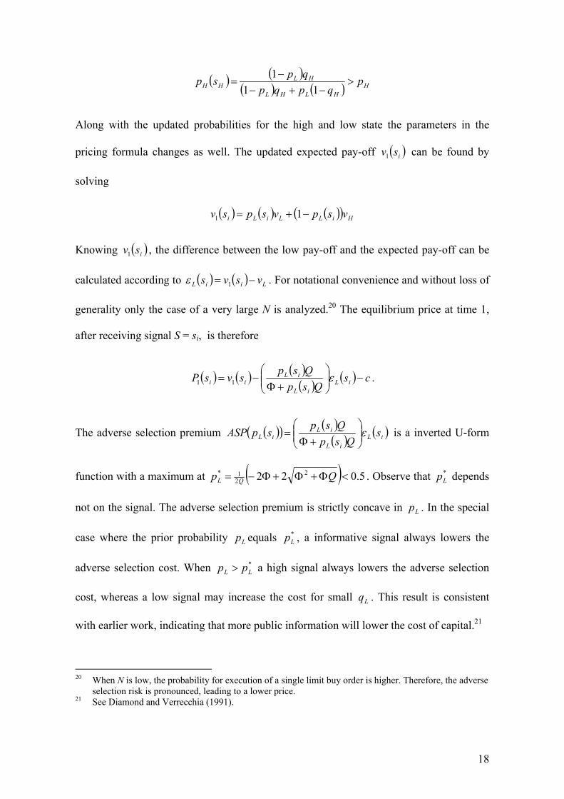
calculated according to ( ) ( ) LiiL vsvs −= 1ε . For notational convenience and without loss of

generality only the case of a very large N is analyzed.20 The equilibrium price at time 1,

after receiving signal S = si, is therefore

( ) ( ) ( )( ) ( ) cs

QspQspsvsP iLiL

iLii −

+Φ

−= ε11 .

The adverse selection premium ( )( ) ( )( ) ( )iL

iL

iLiL s

QspQspspASP ε

+Φ

= is a inverted U-form

function with a maximum at ( ) 5.022 221* <Φ+Φ+Φ−= Qp QL . Observe that *

Lp depends

not on the signal. The adverse selection premium is strictly concave in Lp . In the special

case where the prior probability Lp equals *Lp , a informative signal always lowers the

adverse selection cost. When *LL pp > a high signal always lowers the adverse selection

cost, whereas a low signal may increase the cost for small Lq . This result is consistent

with earlier work, indicating that more public information will lower the cost of capital.21

20 When N is low, the probability for execution of a single limit buy order is higher. Therefore, the adverse

selection risk is pronounced, leading to a lower price. 21 See Diamond and Verrecchia (1991).

19

But most important, the IPO-price at time 0 depends on the two public signals. When the

low signal with likelihood Lq is received, the conditional price at time 1 is

( )( ) ( )( ) ( )( )

( )( )

( )( ) cqsQ

qpqpqp

Qqpqp

qp

qsvqsP LLL

LLLL

LL

LLLL

LL

LLLL −

−−+

+Φ

−−+

−= ε

11

1111

The same holds for the high signal with likelihood Hq :

( )( ) ( )( )

( )( ) ( )

( )( ) ( )

( )( ) cqsQ

qpqpqp

Qqpqp

qp

qsvqsP HHL

HLHL

HL

HLHL

HL

HHHH −

−+−

−+Φ

−+−

−

−= ε

111

111

11

Thus, the best estimation at time 0 for the price at time 1, given Lq and Hq , is

( )[ ] ( )( ) ( )( ) ( ) ( )( )HHHLLLHL qsPsSqsPsSqqPE 1110 PrPr1, =+=−= .

Here, the conditional prices at time 1 are weighted with the probabilities for the low or

high signal. Using Bayes rule once again (see appendix) and solving for the unconditional

probability of a high signal is given by

( ) ( )( )( ) ( )LHHHHH

LHHH spqqsp

spqsS+−

==1

Pr .

Because the adverse selection cost is strictly concave in Lp , informative signals just

before time 1 always lower the expected adverse selection cost, when the expectation is

taken at time 0. Thus, firms should care about the information policy as well as the analyst

and media coverage at the time of the IPO. A higher and credible commitment of a firm to

provide public information will reduce the cost of capital.

20

Example (continued): For the same data as before, the adverse selection cost depending

on the probability of the low state is depicted in figure 5.

Figure 5:

0 0.5 10

2

43.852

0

ASP pL( )

10 pL

The adverse selection cost-function has its maximum at 481.0* =Lp , slightly below 0.5.

For every combination of Hq and Lq the expected adverse selection cost is a convex

combination. Once a informative signal is received, given that the prior probability is

close to *Lp , the adverse selection cost is lowered.

C. Implications for the cross-section of expected returns

At time 0 investors form expectations about how informative the signals about the true

state will be. The precision of public available information may depend on how interesting

the business of the firm is for the public and therefore how large the analyst coverage will

be. Assume that the analyst coverage just before time 1 may be high or low, that is AC =

acj, with j = H,L. Moreover, assume that in the high state the signal is always more

informative then in the low state. The reason may simply be the observation, that firms

and analyst are more reluctant to disseminate bad news.22

22 Hong, Lim, and Stein (2000) argue that bad new “travel slowly” compared to good news. They provide

empirical results which are consistent with that hypothesis. Specifically, they show that low-coverage stocks react more sluggishly to bad news than to good news. In addition, Brennan, Jegadeesh, and Swaminathan (1993) find faster adjustment to new information for stocks with wider analyst following.

21

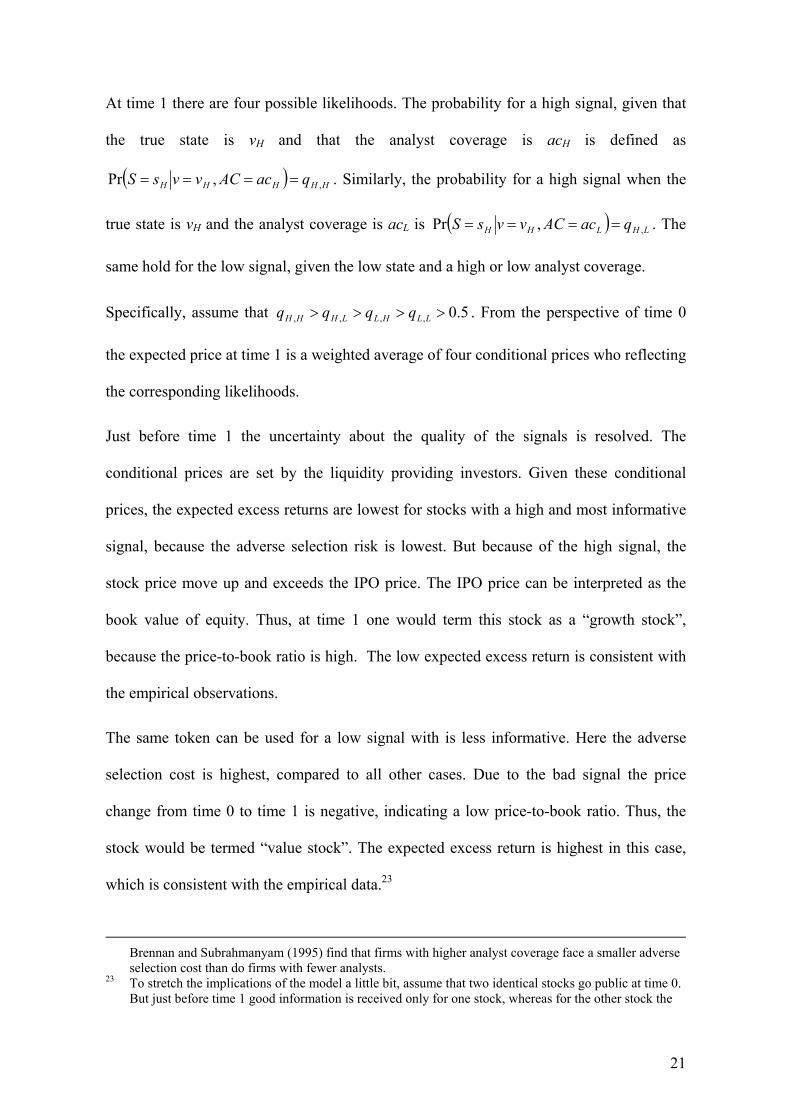
At time 1 there are four possible likelihoods. The probability for a high signal, given that

the true state is vH and that the analyst coverage is acH is defined as

( ) HHHHH qacACvvsS ,,Pr ==== . Similarly, the probability for a high signal when the

true state is vH and the analyst coverage is acL is ( ) LHLHH qacACvvsS ,,Pr ==== . The

same hold for the low signal, given the low state and a high or low analyst coverage.

Specifically, assume that 5.0,,,, >>>> LLHLLHHH qqqq . From the perspective of time 0

the expected price at time 1 is a weighted average of four conditional prices who reflecting

the corresponding likelihoods.

Just before time 1 the uncertainty about the quality of the signals is resolved. The

conditional prices are set by the liquidity providing investors. Given these conditional

prices, the expected excess returns are lowest for stocks with a high and most informative

signal, because the adverse selection risk is lowest. But because of the high signal, the

stock price move up and exceeds the IPO price. The IPO price can be interpreted as the

book value of equity. Thus, at time 1 one would term this stock as a “growth stock”,

because the price-to-book ratio is high. The low expected excess return is consistent with

the empirical observations.

The same token can be used for a low signal with is less informative. Here the adverse

selection cost is highest, compared to all other cases. Due to the bad signal the price

change from time 0 to time 1 is negative, indicating a low price-to-book ratio. Thus, the

stock would be termed “value stock”. The expected excess return is highest in this case,

which is consistent with the empirical data.23

Brennan and Subrahmanyam (1995) find that firms with higher analyst coverage face a smaller adverse selection cost than do firms with fewer analysts.

23 To stretch the implications of the model a little bit, assume that two identical stocks go public at time 0. But just before time 1 good information is received only for one stock, whereas for the other stock the

22

When the ratio of informed trading to expected liquidity trading is high, the probability

which maximizes the adverse selection cost, *Lp can be much lower than 0.5. Given that

the initial, unconditional probability of the low state is 0.5, a relatively uninformative low

signal may push the updated probability closer to *Lp , increasing the adverse selection

cost. In this case the expected excess return of the value stock will be even higher.

The analysis shows that more precise public available information reduces the adverse

selection cost more strongly. When the precision of the signal in the case of good news is

higher the adverse selection cost should be lower compared with the case of bad news.

Thus, stocks who had received good (bad) news in the past should have a high (low)

realized return and a low (high) expected return due to systematic changes in the adverse

selection cost.

Finally, when the analyst or media coverage for large or mid cap stocks is higher, as

empirical evidence suggests, the adverse selection cost should be larger for smaller stocks

on average, linking the results of the model to the size effect.24

D. Allocation of stocks in the IPO

In section A it was assumed the highest bidder is served first in the allocation of stocks to

investors and all investors pay the same IPO price. While such an auction is highly

recommended by theoretic arguments, in real markets other rationing schemes (e.g.

information is bad. Assume further that liquidity seller have some discretion about which stocks they sell at time 1. When they prefer the stock with the good news for selling, more liquidity trading is directed to this stock, meaning that the adverse selection cost of this stock is getting lower. Of course, the adverse selection cost of the other stock will increase. This reinforces the implications for growth and value stocks. Moreover, the stock turnover in the stock with good information should then be higher, compared to the stock with bad information.

24 Stocks with a high ratio of informed trading to liquidity trading have a high information risk in the sense of Aslan et al. (2008). They show that especially smaller firms have a high information risk. The model used here would therefore imply that small value firms should have the highest expected excess return, which is consistent with empirical data provided, e.g., by Fama and French (2007a, 2007b).

23

bookbuilding) are used.25 In this section a simple rationale for not using a common price

auction with a fixed stock supply is presented.

With all assumption of section A still in place, assume now that all shares will be sold to

investors belonging to group B (marginal investors), provided that B > M. Notice that the

reservation price of investors belonging to group A is still higher. Despite this fact, no

shares are allocated to group A.

Because group B investors are the marginal investors, the IPO price should be the same on

the first sight. But now are more stocks allocated to investors of group B, so the expected

number of liquidity sales at time 1 is higher on average, leading to a higher expected price

at time 1. Thus, type B investors are willing to pay a higher IPO-price at time 0, because

they expect better trading conditions which in turn decrease the adverse selection cost at

time 1. That is,

( ) ( ) 0000 1investors B tostocks all allocating PcvcQpM

QpvP BLLB

LB >−−+

−

+

−= λελ

λ .

The proof follows from the fact that ( )BMBM ABB −+> λλλ because AB λλ > .

This basically means that the allocation of stocks only to marginal investors with the

highest propensity to sell at time 1 reduces the expected adverse selection costs at time 1.

But this result strongly depends on the assumption, that trading between time 0 and time 1

is not possible or even forbidden.

Therefore, assume that just after time 0 (say at time 0') stocks may be traded. Suppose that

at time 0' the same information set as at time 0 applies. Thus, at time 0’ is no adverse

25 See for an analysis of bookbuilding procedures in allocation shares to investors Benveniste and Spindt

(1989). For an analysis of different auction types see Biais and Faugeron-Crouzet (2002).

24

selection risk at all. But indeed, the fixed transaction costs must be paid when transacting.

The new timeline of events is depicted in Figure 6.

Figure 6: New timeline of the events

time 0 time 0’ time 1 time 2 (no informational Trading (risk of adverse Liquidation asymmetry) selection)

Because investors belonging to group A did not get shares at time 0, they are willing to

buy shares for their own reservation at time 0’ in the secondary market. Observe that this

price is higher than the IPO-price. Investors belonging to group Β are eager to sell,

because they will expect to make an excess return. But in equilibrium, knowing that they

will get a slightly higher price at time 0', type B investors bid up the IPO-price to a point

when their expected excess return is just zero (after fixed transaction cost). Thus, the firm

going public is indeed able to skim parts of the consumer rent.

The reservation price of type A investors at time 0’ depends on how large the group is:

( ) ( ) ( ) cvcQpAMA

QpvAP ALLBA

LA

A −−+

−

+−+

−= 00'0 1 λελλ

λ

When more stocks change hands at time 0’ from type B investors to type A investors, this

increases the adverse selection cost at time 1, reducing the reservation price. Thus, the IPO

price, the group B investors are willing to pay depends on the how many stocks are traded

at time 0’. The IPO price is therefore a function of the size of group A investors:

25

( ) ( ) ( )

.

1

'0'0

'0000

+

−

=

+

−

−−+

−

+−+

−=

MAP

MAMP

MAP

MAMcvc

QpAMAQpvAP

AB

ABL

LBA

LB

B λελλ

λ

This price is a weighted average consisting of the two reservation prices at time 0’,

weighted by the probability that an investor B will or will not trade at time 0’, that is

MA or ( ) MAM − respectively.

Thus, when stocks in an IPO are predominately allocated to investors with a short holding

horizon and provided that there are only few investors with a long holding horizon,

underpricing may be the common result the first trading day. The theory implies that

underpricing should be negatively related to trading volume.

The model produces a remarkably price pattern for IPO’s. At time 0', the first trading day

after the IPO, one would expect underpricing as long as A < M. Observe that only the

allocation of shares among different types of investors with different investment horizons

matters to produce this outcome. Moreover, the expected price change from time 0’ to

time 1 should be negative on average, because information asymmetries come into play.

When IPO-stocks are predominately small, high risky and getting more and more out of

focus of the public after the IPO, one would expect average prices to decrease slowly due

to an increasing adverse selection premium.

Ritter and Welch (2002) report that for the years 1980 to 2001 the equally weighted

average first day return of IPO’s is 18.8%. It seems fair to say that the model presented

here can not account for that huge first day return. The mechanics of the model may only

help to explain partially the amount of underpricing seen in real markets. But is adds to the

understanding why the allocation of stocks to different investor groups may be important.

26

Example (continued): With the same data as before, figure 7 depicts the prices for three

different allocations of stocks to the two investor groups.

Figure 7:

0 500 1000 1500 200097

97.5

98

98.5

99

99.599.212

97.327

PA A( )

P A( )

PB

P0

2 103×1 A

P0 stands for the price, where group A investors receive full allocation (A = 2000) and the

price is set by marginal investors belonging to group B, receiving M – A shares. In this

example, N →∞. The corresponding price is P0 = 97.33. PB is the price, when all stocks

are allocated to group B investors and if there is no trading before time 1. The price is

P0(allocating all stocks to B investors) = 98.06. P(A) is the IPO price group B investors

are willing to pay, when the amount of A-stocks can be sold to investors belonging to

group A at time 0’. This price varies from ( ) 06.9800 =BP to ( ) 45.9820000 =BP .

Underpricing in figure 7 is measured by the difference between PA(A), the reservation

price of the group A investors at time 0’, and P(A), the IPO price group B investors are

willing to pay, i.e. ( ) ( )APAP BA0'0 − . Underpricing is highest when only very few group A

investors are in the market, i.e. for A = 1 the difference is ( ) ( )11 0'0BA PP − = 1.15.

27

E. Concluding remarks

In this paper a simple stylized market microstructure model in an asymmetric information

framework is studied. Contrary to existing market microstructure models, in this model

liquidity traders only have the need to sell stocks immediately. As a consequence no bid-

ask-spread arises and the whole trading takes place at the bid price. It is shown, that

properly anticipated future transaction costs should be reflected in the stock price.

Whereas the magnitude of direct trading cost (brokerage fee, etc) is rather low, the adverse

selection cost of future liquidity trading can be quite high. Rational investors should

demand a premium as a compensation for the total expected transaction cost before

entering the market at all. It is argued that the adverse selection cost depends on various

market microstructure parameters, such the number of informed traders, the expected

liquidity demand, the potential investor base and the business risk of the firm. Thus, firms

with different market mircostructure characteristics should have different expected returns.

Moreover, the dynamics of the adverse selection cost is driven by information related

factors, such as the information policy of the firm or analyst or media coverage as well as

changing selling needs of liquidity traders. Specifically, it is shown that systematic

differences in adverse selection risk could help to explain observed return differences for

value and growth stocks, without relying in behavioural finance models. The book-to-

market factor as well as the size factor in the Fama and French (1993) asset pricing model

may simply be interpreted as noisy proxies for adverse selection risk.

Further research could focus on the interaction of the adverse selection cost with

endogenous noise trading, which is not rational but information related. Suppose noise

trading demand is triggered only when salient positive, public observable signals arrive in

28

the market.26 Then, trading volume would go up and the adverse selection cost would

decrease, reinforcing the results of this paper. As long as noise trading only affects prices

systematically but indirectly through a changing expose of rational liquidity provider to

adverse selection, markets are informational efficient in the sense of Grossman and

Stiglitz (1980). A theory of endogenous noise trading along that lines may help to explain

the momentum effect27, the interaction between momentum and turnover28, and the

observation that expected returns are lower when turnover volatility is high29, via

systematically changing adverse selection costs and without relying on behavioural biases

influencing prices directly.

26 See Bagehot (1971) or Black (1986) for the notion that noise traders may react to public available

information which is already incorporated in security prices.. 27 See Jegadeesh and Titman (1993). 28 See Lee and Swaminatham (2000). 29 See Chordia, Subrahmanyam, and Anshuman (2001).

29

Appendix

A. Comparative statics for the price at time 1

Given cNQpQNp

QpQNpvP LLL

LL −

Φ+Φ−−−

−−−= ε22

2

01 .

(i) =∂∂

L

Pε

1

Φ+Φ−−−

−−− 22

2

NQpQNpQpQNp

LL

LL <0

Proof: For 01 <∂∂

L

Pε

, ( ) 02 <Φ−Φ N . This implies Φ>N . This condition is fulfilled by

assumption.

(ii)

( ) ( )( ) ( ) 022

222

2

221 <−−

Φ+Φ−−−

−−+

Φ+Φ−−−−−−

=∂∂ QpNp

NQpQNpQpQNp

NQpQNpQpNp

QP

LLLLL

LLL

LL

LL εε

Proof: This is equivalent to ( )( ) 022

2

<Φ+Φ−−−

−−+− L

LL

LLL NQpQNp

QpQNp εε . It remains to show

that

( )( ) 122

2

<Φ+Φ−−−

−−NQpQNp

QpQNp

LL

LL . If 02 =Φ−Φ N , the term is 1. Therefore, 02 <Φ−Φ N

or Φ>N , which is fulfilled by assumption.

(iii) ( ) ( ) 02222

21 >−Φ

Φ+Φ−−−

−−=

Φ∂∂ N

NQpQNpQpQNpP

L

LL

LL ε

Proof: Because 02 <−Φ N by assumption and the nominator is negative, the derivative

must be negative since the denominator is always positive.

30

(iv) 011 <−=∂∂

cP . The proof is obvious.

B. Proof that the adverse selection cost decreases when N is increasing.

The derivative of the adverse selection cost with respect to N is

( )( ) 0222

2

22 <Φ−−Φ+Φ−−−

−−−

Φ+Φ−−−−

=∂∂ Qp

NQpQNpQpQNp

NQpQNpQp

NASC

L

LL

LL

LL

L .

This is equivalent to ( )( ) 011 22

2

<Φ+Φ+Φ−−−

−−−

NQpQNpQpQNp

LL

LL . When Φ > 1 and Φ>N ,

the adverse selection cost decreases as N increases. This is fulfilled by assumption.

C. Calculation of the unconditional probability for signal S = sH.

Bayes rule implies that

( ) ( ) ( )( ) ( ) ( ) ( )LHLHHH

HHHHH sSvvsSsSvvsS

sSvvsSvvsS

===+======

===PrPrPrPr

PrPrPr

Given the notation in the paper ( ( )HHH vvsSq === Pr , ( ) ( )HHHH sSvvsp === Pr , and

( ) ( )LHLH sSvvsp === Pr ) , this can be written as

( ) ( )( ) ( ) ( )( ) ( )LHHHHH

HHHH spsSspsS

spsSq=−+=

==

Pr1PrPr

Solving for ( )HsS =Pr yields

( ) ( )( )( ) ( ) HLHHHH

LHHH qspqsp

spqsS+−

==1

Pr .

Observe that ( ) ( )HL sSsS =−== Pr1Pr .

31

References

Admati, Anat and Paul Pfleiderer, 1988, A Theory of Intraday Patterns: Volume and Price

Variability, in: Review of Financial Studies, 1, 3-40.

Akerlof, George A. (1970), The Market for "Lemons": Quality Uncertainty and the

Market Mechanism, in: Quarterly Journal of Economics, 84, 488-500.

Allen, Franklin and Gary Gorton, 1992, Stock Price Manipulation, Market Microsturcture

and Asymmetric Information, in: European Economics Review, 36, 624-630.

Amihud, Yakov, 2002, Illiquidity and Stock Returns: Cross-section and Time Series

Effects, in: Journal of Financial Markets, 5, 31-56.

Amihud, Yakov and Haim Mendelson, 1986, Asset Pricing and the Bid-Ask Spread, in:

Journal of Financial Economics, 17, 223-249.

Amihud, Yakov and Haim Mendelson, 1989, The Effect of Beta, Bid-Ask Spread,

Residual Risk, and the Size on Stock Returns in: Journal of Finance, 44, 479-486.

Amihud, Yakov, Haim Mendelson, and Lasse H. Pedersen, 2005, Liquidity and Asset

Prices, in: Foundations and Trends in Finance, 1, 269-364.

Arbel, Avner and Paul Strebel, 1981, The Neglected and Small Firm Effect, in: The

Financial Review, 201-218

Aslan, Hadiye, David Easley, Soeren Hvidkjaer, and Maureen O’Hara, 2008, Firm

Characteristics and Informed Trading: Implications for Asset Pricing, Working Paper

Bagehot, Walter, 1971, The only game in town, in: Financial Analyst Journal, 27, 12-14.

Banz, Rolf, 1981, The Relationship between Return and Market Value of Common

Stocks, in: Journal of Financial Economics, 9, 3-18.

Benveniste, Lawrence M. and Paul A. Spindt, 1989, How investment bankers determine

the offer price and allocation of new issues, in: Journal of Financial Economics, 24,

343-363.

Bhushan, Ravi, 1989, Firm Characteristics and Analyst Following, in: Journal of

Accounting and Economics, 11, 255-274.

Biais, Bruno and Anne Marie Faugeron-Crouzet, 2002, IPO Auctions: English, Dutch, …

French, and Internet, in: Journal of Financial Intermediation, 11, 9-36.

32

Black, Fischer, 1986, Noise, in: Journal of Finance, 41, 529-543.

Booth, James R. and Lena Chua, 1996, Ownership dispersion, costly information, and IPO

underpricing, in: Journal of Financial Economics, 41, 291-310.

Brennan, Michael J., N. Jegadeesh, and B. Swaminathan, 1993, Investment Analysis and

the Adjustment of Stock Prices to Common Information, in: Review of Financial

Studies, 6, 799-824.

Brennan, Michael J., and Avanidhar Subrahmanyam, 1995, Investment Analysis and Price

formation in Securities Markets, in: Journal of Financial Economics, 38, 361-381

Brennan, Michael J., and Avanidhar Subrahmanyam, 1996, Market Microsturcture and

Asset Pricing: On the Compensation for Illiquidity in Stock Returns, in: Journal of

Financial Economics, 41, 441-464´

Brennan, Michael J., Tarun Chordia, and Avanidhar Subrahmanyam, 1998, Alternative

Factor Specifications, Security Characteristics, and the Cross-section of Expected

Stock Returns, in: Journal of Financial Economics, 49, 345-373.

Chalmers, John M., and Gregory B. Kadlec, 1998, An Empirical Examination of the

Amortized Spread, in: Journal of Financial Economics, 48, 159-188.

Chordia, Tarun, Avanidhar Subrahmanyam, and V.R. Anshuman, 2001, Trading Activity

and Expected Stock Returns, in: Journal of Financial Economics, 59, 3-32.´

Datar, Vinay T., Narayan Y. Naik, and Robert Radcliffe, 1998, Liquidity and Stock

Returns: An Alternative Test, in: Journal of Financial Markets, 1, 203-219.

Diamond, Douglas and Robert E. Verrecchia, 1991, Disclosure, Liquidity, and the Cost of

Capital, in: Journal of Finance, 46, 1325-1359.

Easley, David and Maureen O'Hara, 1987, Price, Trade Size, and Information in Securities

Markets, in: Journal of Financial Economics, 19, 69-90.

Easley, David and Maureen O'Hara, 2004, Information and the Cost of Capital, in: Journal

of Finance, 59, 1553-1583.

Easley, David, S. Hvidjkaer, and Maureen O'Hara, 2002, Is Information Risk a

Determinant of Asset Returns, in: Journal of Finance 57, 2185-2221.

33

Eleswarapu, V.R., 1997, Cost of Transacting and Expected Returns in the Nasdaw Market,

in: Journal of Finance, 52, 2113-2127.

Eleswarapu, V.R., and Marc R. Reinganum, 1993, The Seasonal Behavior of Liquidity

Premium in Asset Pricing, in: Journal of Financial Economics, 34, 373-386

Fama, Eugene F. and Kenneth R. French, 1992, The Cross-Section of Expected Returns,

in: Journal of Finance, 51, 1405-1436.

Fama, Eugene F. and Kenneth, R. French, 1993, Common Risk Factors in the Returns on

Stocks and Bonds, in: Journal of Financial Economics, 33, 3-56.

Fama, Eugene F. and Kenneth R. French, 2007a, Migration, in: Financial Analyst Journal,

63, no. 3, 48-58.

Fama, Eugene F. and Kenneth R. French, 2007b, The Anatomy of Value and Growth

Stock Returns, in: Financial Analyst Journal, 63, no. 6, 44-54.

Garleanu, Nicolae and Lasse H. Pedersen, 2004, Adverse Selection and the Required

Return, in: Review of Financial Studies 17, 643-665.

Glosten, Lawrence R., and Paul R. Milgrom, 1985, Bid, Ask, and Transaction Prices in a

Specialist Market with Heterogeneously Informed Traders, in: Journal of Financial

Economics, 14, 71-100.

Grossman, Sanford and Joseph E. Stiglitz, 1980, On the impossibility of informationally

efficient markets, in: American Economic Review, 70, 393-408.

Hong, Harrison, Terence Lim, and Jeremy C. Stein, 2000, Bad News travel slowly: Size,

Analyst Coverage, and the Profitability of Momentum Strategies, in: Journal of

Finance, 55, No. 1, 265-295.

Jegadeesh, Narasimhan, and Sheridan Titman (1993), Returns to buying winners and

selling losers: Implications for Stock market efficiency, in: Journal of Finance, 48, 65-

91.

John, Kose and Ranga Narayanan, 1997, Market Manipulation and the Role of Insider

Trading, in: Journal of Business, 70, 217-247.

Lakonishok, Josef, Andrej Shleifer, and Robert Vishny, 1994, Contrarian Investment,

Extrapolation, and Risk, in: Journal of Finance, 49, 1541-1578.

34

Lee, Charles M.C. and Bhaskaran Swaminathan (2000), Price Momentum and Trading

Volume, in: Journal of Finance, 55, 2017-2069.

Kyle, Albert S., 1985, Continuous Auctions and Insider Trading, Econometrica, 53, 1316-

1335.

Milgrom, Paul R. and Nancy Stockey, 1982, Information, Trade and Common

Knowledge, in: Journal of Economic Theory, 26, 17-27.

O'Hara, Maureen, 1995, Market Microstructure Theory, Blackwell, Cambridge, Mass.

Pastor, Lubos and Robert Stambaugh, 2003, Liquidity Risk and Stock Returns, in: Journal

of Political Economy, 111, 642-685.

Ritter, Jay, and Ivo Welch, 2002, A Review of IPO Activity, Pricing, and Allocations,

NBER Working Paper Series, Working Paper 8805.

Wang, J., 1993, A Model of Intertemporal Asset Prices Under Asymmetric Information,

Review of Economic Studies, 60, 249-282.