northfield transaction cost · pdf file3 transaction cost model the essence of a traded...

TRANSACTION COSTCost Model

NORTHFIELD

IDENTIFY

ANALYZE

QUANTIFY

Transaction Cost Model

1 www.northinfo.com

FEB-3-2015

Table of Contents INTRODUCTION ............................................................................................................................. 2

DISCUSSION OF TRADING COSTS .................................................................................................... 3

MARKET IMPACT BASICS ............................................................................................................... 4

MARKET IMPACT FOR DUMMIES! .................................................................................................... 4

ESTIMATING “TAKEOVER” MARKET IMPACT EMPIRICALLY ................................................................ 6

ESTIMATING LIQUIDITY GLOBALLY USING OUR US MODEL ............................................................... 7 Impact Decay ....................................................................................................................... 9 Crowding ............................................................................................................................ 11 Coverage ............................................................................................................................ 12 File Name, Location and How to Load it into the Optimizer .......................................... 12 File Format ......................................................................................................................... 13

REFERENCES ............................................................................................................................... 13

WHY NORTHFIELD IS RIGHT FOR YOU ............................................................................................ 15 Powerful, Integrated, Consistent & Comparable Risk Models ....................................... 15 Open Models: Open Systems. No Black Boxes! ............................................................. 15 Global, Regional, Country & Asset Coverage ................................................................. 15 Sophisticated, Flexible, Robust, Open Analytical Systems ............................................ 15 Partners .............................................................................................................................. 15 Innovation .......................................................................................................................... 15 Excellent Training, Support and Solutions ...................................................................... 15

2 www.northinfo.com


During August of 2007, stock markets around the world experienced extremely unusual return events. Numerous funds that had experienced losses in mortgage securities were forced to sell equity securities to meet margin calls, creating a dramatic imbalance between the number of willing sellers and buyers for some securities. This lead to falling prices for some equities and another cycle of margin related forced selling. Since these events, investors, particularly those with a quantitative approach to investment decisions, have been focusing on liquidity concerns.

There are a number of other market trends that are creating the need for a better understanding of how liquidity imbalances translate into trading costs and their impact on market prices. Algorithmic trading methods, which require an explicit forecast of market impact, continue to garner an increasingly large share of trading volume in developed markets. In addition, investors are increasingly participating in “frontier” markets with very low liquidity levels causing severe capacity constraints on the amount of capital employed. Finally, the growth of hedge funds has increased trading volumes dramatically, as these funds average something more than five times the turnover that traditional funds do.

There is an extensive amount of literature on how to predict the extent to which the introduction of a trade of a particular size will impact prices of a stock. Numerous models exist both in the academic literature and within the practitioner community. However, empirical estimation and validation of such models has been published only for US data, with essentially nothing available on other global stock markets.

There are a variety of trends in today’s global stock markets that are creating large amounts of concern about liquidity. For the purposes of investors, we believe the correct way to view liquidity is as the degree of price change that may be expected from the initiation of a trade of a given magnitude. Existing models of liquidity have not been empirically explored to a meaningful degree outside the US.

While the functional form of market impact models is well agreed upon by researchers, the empirical estimation of the parameters has often lacked the boundary conditions which we find to be of critical importance. We present an information leakage rationale to justify the mechanism of our boundary conditions. Our market impact model for US stocks shows a very high degree of explanatory power.

We also present a mechanism by which the cost estimates of any market impact model can be extended from one data set to another by using positive serial correlation as a proxy for illiquidity. The relationship between expected trade costs and positive serial correlation of returns across capitalization deciles of US stocks is shown to be almost exactly linear (R-squared over 90%). This should allow for at least reasonable estimation of market impact for those markets where databases of explicit trade data are insufficient or unavailable.

Introduction

3 www.northinfo.com


The essence of a traded asset’s liquidity hinges on the cost of trading a particular quantity of that asset. The question is not really about whether you can trade, but rather how much change in the price must be absorbed in order to induce other market participants to take the other side of the trade you wish to do. We refer to this required change in price as market impact.

When we consider the overall cost of trading an asset, there are several components. The first is agency costs, the fees charged by brokers, exchanges and custody banks for actually executing the transaction. The second is bid/asked spread, the value difference between the prices at which liquidity providers such as market makers and exchange specialists are willing to buy and sell. The third component is the aforementioned market impact, the extent to which my trade requires change in the asset price in order to execute the desired quantity. The fourth cost is what traders call trend cost, or what portfolio managers might think of as risk. It is simply the price change that occurs due to the trading of other market participants between the time when I decide to trade and when my trade is actually executed. It should be noted that trend costs may be negative (a price may move in my favor).

There are two often overlooked ingredients to trading costs. The first is the issue of cross-market impact. If I am buying a large amount of a particular stock, say General Motors, my trade will impact the price of GM. To the extent that the relative value of other similar stocks such as Ford or Toyota are estimated by investors in comparison to GM, the market price of Ford or Toyota may also be impacted. Finally, we must also consider the opportunity costs of the time it takes to execute our transactions. Unless we are investing passively, we want to buy stocks before they go up, not after. Similarly, if we’re selling we want to sell before they go down, not after.

In framing a discussion of liquidity and market impact, we always consider the dimension of time in the context of whether market impact is permanent or temporary. If our trades in any given stock are far apart in time, price movements caused by our trades will be independent of one another. If our trades follow each other with little time in between, market impact effects will have a cascading effect as each trade moves the price from where the previous trade left it. We call this persistent portion of market impact stickiness, and account for it in deciding how quickly to trade.

One way to think of the issue of market impact permanence is to build on the concept of a participation rate. For example, if we trade a stock in a quantity that is 5% of a typical day’s trading volume, that trade will represent 2.5% of the expected volume over two days, 1.25% of the expected volume over four days and .5% of the expected volume over ten days. Eventually, the price influence of our trade exponentially decays to zero.

The empirical estimation of trading costs is difficult. Agency costs are essentially known in advance. Bid/Asked spreads are reasonably stable under normal market conditions but can widen substantially in periods of market

Discussion of Trading Costs

4 www.northinfo.com


stress. The determinants of variation in bid/asked spreads have been well explored in Menya and Paudyal (1996, 2000) and Chorida, Roll and Subrahmanyam (2000).

An extensive array of market impact models have been proposed in the academic literature and brokerage firms. Among these are: Almgren and Chriss (2000), Ferstenberg (2000) and Cox (2001). Most models take the form:

E [M] = α Sπ (1)

Where E[M] is the expected value of the price movement in % S is the quantity of shares to be traded

α, π are parameters fitted from empirical data In most models, the α parameter varies stock by stock and represents the different levels of liquidity across stocks. The π parameter is typically singly estimated for an entire market. It has been speculated that the π parameter may different from market to market due to differences in exchange structure, the balance of institutional versus individual investment in stocks and the existence of alternative trading venues such as electronic crossing networks. Most studies suggest values for π of either one or one half. It should also be noted that we can easily scale the α parameter to rescale the size of the trade S into units of percentage of expected daily volume, as traders often prefer. In order to accommodate models of this kind, the optimization tool our firm makes commercially available allows for either popular value of π, or a weighted combination of the linear and square root processes:

M = [(Bi*St) + (Ci*| St0.5| )] + … (2)

We can also think of these two coefficients, B and C as being a weighted representation of the α parameter. These coefficients represent the elasticity of the asset price with respect to trade magnitudes and hence are the true representation of liquidity.

Bi = W*α Ci = (1-W)*α Unfortunately, when the available market impact models were utilized with the optimization tool, bizarre results were sometimes observed. For example, one model predicted that to sell 10% of the shares outstanding of a US small cap stock (market capitalization $500 million), the expected trading cost would be over 100% of the value. We believe these results arose because the model coefficients were based on empirical estimations from data sets that did not contain large trades because traders considered them too costly. Coefficients for B and C must be estimated under boundary

Market Impact Basics

Market Impact for Dummies!

5 www.northinfo.com


conditions that provide rational results in the entire range of potential trade size from zero to all the shares of a firm. Traders are very concerned that market impact effects are driven by information leakage. Once liquidity providers know what a particular investor is doing in terms of buying or selling particular securities, they will reset the prices at which they are willing to transact in order to maximize their profits. Let us consider a hostile takeover as the “worst case” scenario for market impact: we’re going to buy up all the shares of a company and tell the entire world we’re doing it. The takeover premium can be viewed as an extreme case of market impact. If we believe only in the linear market impact process, we can set our coefficient to the expected takeover premium for a stock divided by shares outstanding. If we believe only in the square root process for market impact, we can set our coefficient to the expected takeover premium for a stock divided by the square root of shares outstanding. If we don’t know which process to believe in, we can just do both with a weighting summing to one.

Bi = W * ( E[Pi] / Si) (3) Ci = (1-W) * E[Pi] / (Si

0.5) (4)

Bi = the coefficient on the linear process Ci = the coefficient on the square root process Pi = the takeover premium in percent Si = the number of shares outstanding W = a weight estimated from empirical data

To turn this simple estimation into a more complete model, we incorporate two additional features. First, we must consider differences in liquidity across different stocks. Secondly, we must recognize that our model based on takeover premiums represents the boundary condition of a “worst case” scenario for information leakage. Normal trading involves much smaller information leakage effects. If we assume takeover premiums are lognormal, we can easily express the expected takeover premium as a function of a liquidity measure E[Pi] = QP / (( 1 + K/100)Zi) (5) P = % average price premium in a hostile takeover K = the log percentage standard error around P Zi = the Z score of a liquidity measure for stock I Q = a scalar between zero and one Let us do a quick example with some stylized facts: Various academic studies using M & A databases have reported average takeover premiums from 37 to 50% with a standard deviation around 30%.

6 www.northinfo.com


We will consider a hypothetical company with $5 billion market cap, $50 share price and 100 million shares outstanding. Assuming P = 37, K = 40, W = .25, Zi = 0, we would get a cost of 2.88% for a 1,000,000 share trade impact = 2.88% and .27% for a 10,000 share trade. Implicit in this estimation is that the trades are done over a time period which is comparable to the time period over which stock prices react to the release of the news of hostile takeover (perhaps a day or two). To the extent we trade more slowly over a longer time period, the market impact costs would be reduced. If we take our estimates of the P and K parameters from the finance literature on hostile takeovers, we need only estimate the Q and W parameters relative to whatever fundamental information we wish to use as Z. In order to facilitate empirical estimation, a dataset of actual trades was obtained from Instinet. This data set included over 1.5 million orders over an 18 month period with fine detail such as time stamps, arrival price, execution price, order type (buy/sell, limit/market), tracking of cancelled orders, etc. The information was anonymous. We have no information on what firms traded or which orders belong to whom. Almost all of the data was from the US, with some small representation of major markets such as Japan, UK, Canada, etc. Obviously this is a very large data set over which to estimate a model with only two free parameters. We choose to explain the differences in liquidity levels across stocks using three characteristics: the log of market capitalization of the stock, the ratio of average daily volume to shares outstanding, and the inverse of the security’s volatility. Each of these three characteristics is standardized into a Z-Score across our estimation universe of US stocks, and then the three values are combined in a weighted average. Our final preparatory step is to define how we are going to measure the market impact of individual trades. One way to measure market impact would be to compare the price we got on our trade versus the price on the previous trade as a measure of how much our trade “moved the price.” However, this measure may not be relevant to us. We care about how much the price moved from the price it was at when we decided to trade the stock, which we call the arrival price. It’s the percentage in price between the execution price and the price that existed in the market when we got the order to transact the stock. This representation is consistent with the concept of “Implementation Shortfall” described in Perold (1988). A grid search method was employed to identify the “best fit” values of Q and W over a set of 1.2 million US market orders. The choice of the Q and W pair was based on the trade dollar weighted goodness of fit (R-squared) and the requirement that the model not exhibit statistically significant bias (i.e. the average forecast has to fit the average cost). Unlike an OLS regression, the grid search does automatically produce a best linear unbiased estimate.

Estimating “Takeover”

Market Impact Empirically

7 www.northinfo.com


We chose to use a trade dollar weighted R-squared as traders obviously care a lot more about getting this right when doing million share trades as compared to hundred share trades. The dollar weighted time interval between arrival of an order and its termination (either filled or cancelled) was approximately ninety minutes, illustrative of the fact that large institutional orders were involved. If we continue our use of 37% to represent P, the central tendency of the takeover premium, we obtained a best pair of Q = .594 and W = .650. The trade dollar weighted R-squared was 74%. The R-squared values were fairly insensitive to the choice of Q and W and other combinations also produced very high degrees of fit. These parameters will be updated from time to time using trade cost data published by investment banks and from our ongoing research that studies market impact with “tick by tick” methods. Unfortunately, our Instinet trade database contained insufficient observations on non-US markets to proceed with the above model. In order to extend our results to other stock markets we would have to use other methodologies. Our first effort to extend our results to global markets is based on the hypothesis that one of the observable manifestations of illiquidity is positive serial correlation in high frequency returns. The simple intuition is that when information arrives to the market that changes the value of a stock, limited liquidity will not permit everyone who wishes to transact to do so in the initial period following the news. Some people have to transact in the second and subsequent periods, inducing positive serial correlation to the returns. A more formal rationale for this effect is presented in Getmansky, Lo and Makarov (2004). There are numerous statistical methods for the estimation of serial correlation, including autoregressive models and variance ratio tests. Due to the lack of normality in high frequency returns as described in diBartolomeo (2007), we chose to use a non-parametric “runs” test (Wald-Wolfowitz). The logic is simple: if a stock trades liquidly, there should still be a roughly 50% chance it will go up or down tomorrow, irrespective of whether it went up or down today. We should see the sign of daily returns change 50% of the time from one day to the next. If the trading is illiquid, the number of sign changes will be less than 50%. To extend our model, we first created a “seed sample” of US stocks broken into ten deciles of market capitalization. The sample included over 1500 random stocks ranging all the way down to very illiquid shares traded on the NASDAQ “Bulletin Board” and in the “pink sheets.” For each group, we calculated the average Z value of the members for the US market impact model presented above, and produced an estimated average cost to trade 1% of shares outstanding in one trading day. We chose to use 1% of shares outstanding, rather than a percentage of average daily volume because for some of the illiquid stocks, the number of shares traded is so small that a

Estimating Liquidity

Globally using our US Model

8 www.northinfo.com


small percentage of that value would be imperceptibly small to an institutional investor. These values are presented on the center column of Table 1.

Table 1

Market Cap

Deciles

Cost for 1% Shares Out

Trade in One Day

Avg. # of Return “Non-Changes”

in 200 Days 1 .77 97.15

2 .97 100.75

3 1.15 98.07

4 1.28 100.94

5 1.46 101.77

6 1.71 105.29

7 2.00 107.48

8 2.44 111.03

9 3.32 112.56

10 4.98 117.49

We then calculated 200 trading days of daily returns for each stock for a period ending in July of 2008. The number of sign changes for the daily returns was counted. If a stock return was zero for the trading day, this was considered a “non-change” in the sign of the return. The average number of non-changes in return sign is also presented in Table 1. Obviously, there is a strong relationship between the expected costs from our model and the average number of return sign “non changes.” An OLS regression of the two data sets yielded the equation below, with an R-squared of over 90%.

Y = -0.1716 + 0.0018X (6)

Where Y is the fitted value for the estimated cost of a 1% of shares outstanding

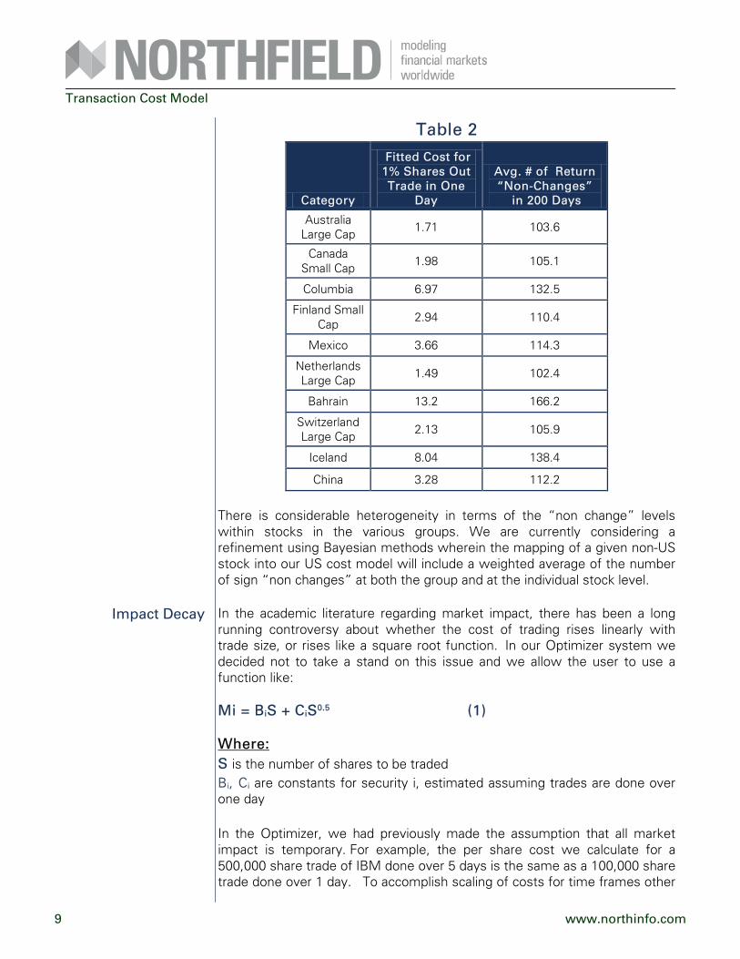
trade in one day X is the average number of daily return sign non-changes in 200 trading days Our next step was to take a sample of approximately forty-five hundred stocks in sixty-seven non-US countries. For large developed markets, we broke the stocks into three categories of capitalization (large, medium, and small) and took a random stratified sample for each category (equal numbers of stocks within each group within a country). Small countries were broken into two categories (large, small) and very small markets (less than 50 issues traded) were kept as one category. We then calculated the number of return sign “non-changes” in the same fashion as for the US. It was then possible to use the equation above to calculate the expected cost for trades according to our model. In Table 2, we present data similar to Table 1 but for some groups of non-US stocks.

9 www.northinfo.com


Table 2

Category

Fitted Cost for 1% Shares Out Trade in One

Day

Avg. # of Return “Non-Changes”

in 200 Days

Australia Large Cap 1.71 103.6

Canada Small Cap 1.98 105.1

Columbia 6.97 132.5

Finland Small Cap 2.94 110.4

Mexico 3.66 114.3

Netherlands Large Cap 1.49 102.4

Bahrain 13.2 166.2

Switzerland Large Cap 2.13 105.9

Iceland 8.04 138.4

China 3.28 112.2

There is considerable heterogeneity in terms of the “non change” levels within stocks in the various groups. We are currently considering a refinement using Bayesian methods wherein the mapping of a given non-US stock into our US cost model will include a weighted average of the number of sign “non changes” at both the group and at the individual stock level. In the academic literature regarding market impact, there has been a long running controversy about whether the cost of trading rises linearly with trade size, or rises like a square root function. In our Optimizer system we decided not to take a stand on this issue and we allow the user to use a function like: Mi = BiS + CiS0.5 (1) Where: S is the number of shares to be traded Bi, Ci are constants for security i, estimated assuming trades are done over one day In the Optimizer, we had previously made the assumption that all market impact is temporary. For example, the per share cost we calculate for a 500,000 share trade of IBM done over 5 days is the same as a 100,000 share trade done over 1 day. To accomplish scaling of costs for time frames other

Impact Decay

10 www.northinfo.com


than one day, we introduced a scaling function based on the number of days over which the trade will be completed. Mi = (Bi/G) S + (Ci/G0.5) S0.5 (2) Where G = number of days required for the trade (note fractional days are permissible) The assumption that all market impact is temporary is quite common. For example, see Ed Qian’s presentation at our 2007 conference in Key Largo, http://www.northinfo.com/documents/261.pdf. The underlying conceptual issue is whether the price impact of a trade is merely related to the need to change the balance of current supply and demand to create a transaction (price impact is temporary), or whether the price impact arises because other market participants observe your trade, assume you know something they don’t, and revise their estimates of the value of the security (price impact is permanent). We have often referred to this degree of permanence based on “information leakage” in market impact as “stickiness.” If we believe that all market impact is temporary, traders who are trying to trade large quantities will stretch out their trades over longer time periods, and the costs will decline proportionately as described in Equation 2. If all impact was permanent, stretching the trade out over longer time periods would not reduce costs. Most people believe that small trades will have only temporary impact, while large trades will have some permanent impact, suggesting that small trades (too small to be noticeable) will act more like the square root process while big trades will be more linear although the slope for very large trades is hard to identify since there is little empirical data. After reviewing the extensive empirical data from various brokerage firms, we believe:

1. For a fixed time interval (say 1 day), the cost of large trades in a given stock rises about linearly with trade size. If you trade five times as many shares, the per share cost increases by about five times.

2. As the time period for the trade increases, the costs decline but at a less than linear relationship. For example, taking five times as long to do a trade cuts the cost by a factor of about three.

These facts point out a way to reconcile the empirical controversy between trading costs being linear or a square root function. In studying the empirical data, it appears that the controversy is more a semantic or conceptual problem than a matter of estimating an accurate empirical model. It appears

http://www.northinfo.com/documents/261.pdf



that costs of large trades are largely linear if we are talking about fixed time frames, while per share costs appear to increase at a decreasing rate (i.e. square root or close to it) if we allow traders to spread the trades out over time frames of their choosing, as some of the impact is permanent and some is temporary. To incorporate this aspect of market impact into the Optimizer, we have created an “impact decay” function.

Mi = (Bi/GR) S + (Ci/(G(0.5*R))) S0.5 (3) Where R is a constant describing the proportion of temporary versus permanent market impact, R≤1 Based on an examination of empirical trading data, we believe a default value of around .71 for R is reasonable. “Crowding” occurs when many managers want to buy or sell the same stock at the same time. It can occur because they use similar assumptions about the covariance among securities, or because they are responding to the same news about the company. The cost of trading will rise during periods when crowding is prevalent. If you believe that you will be trading in “crowded” conditions, you should consider how large your fund is compared to other similar funds. For example, if you believe that your portfolio represents 5% of the total assets being managed using a particular strategy, it is theoretically possible that your trades will be concurrent with trades from the other portfolios representing the other 95%. While it is certainly unlikely that all funds of a given strategy will try to execute identical trades at the same time, your estimates of transaction costs should reflect an expectation of increased costs during such periods. The potential for crowding impacts the amount of capital that can be employed in a particular strategy. An excellent reference on the issue of capacity for active strategies is “The Capacity of An Equity Strategy” by Marco Vangelisti (Journal of Portfolio Management, Winter 2006). In order to compensate for crowding while optimizing portfolios, you can appropriately increase the transaction cost coefficients (whether provided by Northfield or other sources). You can also use the shortcut of downward biasing your available time to completion of a trade, which has the same algebraic effect as raising the cost coefficients. For example, if you want to trade 200,000 shares of IBM in two days and you expect crowding, you can set the number of days to trade to 0.5 which will effectively make the trade more expensive.

Crowding



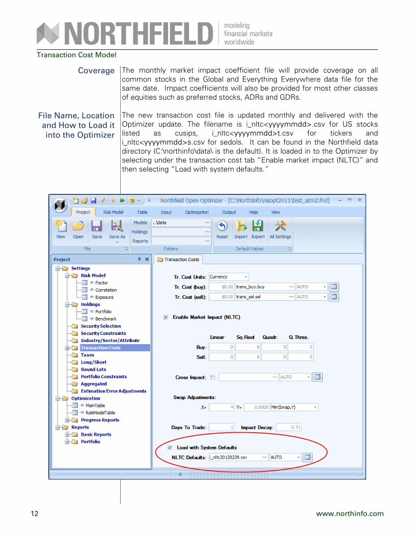
The monthly market impact coefficient file will provide coverage on all common stocks in the Global and Everything Everywhere data file for the same date. Impact coefficients will also be provided for most other classes of equities such as preferred stocks, ADRs and GDRs. The new transaction cost file is updated monthly and delivered with the Optimizer update. The filename is i_nltc<yyyymmdd>.csv for US stocks listed as cusips, i_nltc<yyyymmdd>t.csv for tickers and i_nltc<yyyymmdd>s.csv for sedols. It can be found in the Northfield data directory (C:\northinfo\data\ is the default). It is loaded in to the Optimizer by selecting under the transaction cost tab “Enable market impact (NLTC)” and then selecting “Load with system defaults.”

Coverage

File Name, Location and How to Load it into the Optimizer



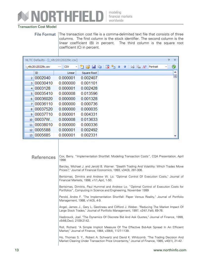
The transaction cost file is a comma-delimited text file that consists of three columns. The first column is the stock identifier. The second column is the linear coefficient (B) in percent. The third column is the square root coefficient (C) in percent.

Cox, Berry. “Implementation Shortfall: Modeling Transaction Costs”, CQA Presentation, April 1998

Barclay, Michael J. and Jerold B. Warner. "Stealth Trading And Volatility: Which Trades Move Prices?," Journal of Financial Economics, 1993, v34(3), 281-306.

Bertsimas, Dimitris and Andrew W. Lo. "Optimal Control Of Execution Costs," Journal of Financial Markets, 1998, v1(1,Apr), 1-50.

Bertsimas, Dimitris, Paul Hummel and Andrew Lo. “Optimal Control of Execution Costs for Portfolios”, Computing in Science and Engineering, November 1999

Perold, Andre F. "The Implementation Shortfall: Paper Versus Reality," Journal of Portfolio Management, 1988, v14(3), 4-9.

Angel, James J., Gary L. Gastineau and Clifford J. Weber. "Reducing The Market Impact Of Large Stock Trades," Journal of Portfolio Management, 1997, v24(1,Fall), 69-76.

Hasbrouck, Joel. "The Dynamics Of Discrete Bid And Ask Quotes," Journal of Finance, 1999, v54(6,Dec), 2109-2142.

Roll, Richard. "A Simple Implicit Measure Of The Effective Bid-Ask Spread In An Efficient Market," Journal of Finance, 1984, v39(4), 1127-1139.

Ho, Thomas S. Y., Robert A. Schwartz and David K. Whitcomb. "The Trading Decision And Market Clearing Under Transaction Price Uncertainty," Journal of Finance, 1985, v40(1), 21-42.

File Format

References



Almgren, Robert and Neil Chriss. “Optimal Execution of Portfolio Transactions”, Journal of Risk, 2001, v3, 5-39

Almgren, Robert and Neil Chriss, “Optimal Execution with Non-Linear Impact Costs and Trading Enhanced Risk”. Working Paper 2001

Malamut, Roberto. “Multi-Period Optimization Techniques for Trade Scheduling”, QWAFAFEW New York, April 2002

Walkling, Ralph A. "Predicting Tender Offer Success: A Logistic Analysis," Journal of Financial and Quantitative Analysis, 1985, v20(4), 461-478.

Billett, Matthew T. and Mike Ryngaert. "Capital Structure, Asset Structure And Equity Takeover Premiums In Cash Tender Offers," Journal of Corporate Finance, 1997, v3(2,Apr), 141-165.

Eckbo, B. Espen and Herwig Langohr. "Information Disclosure, Method Of Payment, And Takeover Premiums: Public And Private Tender Offers In France," Journal of Financial Economics, 1989, v24(2), 363-404.

Walkling, Ralph A. and Robert O. Edmister. "Determinants Of Tender Offer Premiums," Financial Analyst Journal, 1985, v41(1), 27,30-37.

Wansley, James W., William R. Lane and Salil Sarkar. "Managements' View On Share Repurchase And Tender Offer Premiums," Financial Management, 1989, v18(3), 97-110.

Chordia, Tarun, Richard Roll and Avanidhar Subrahmanyam. "Co-Movements In Bid-Ask Spreads And Market Depth," Financial Analyst Journal, 2000, v56(5,Sep/Oct), 23-27.

Menyah, Kojo and Krishna Paudyai. "The Components Of Bid--Ask Spreads On The London Stock Exchange," Journal of Banking and Finance, 2000, v24(11,Nov), 1767-1785.

Menyah, Kojo and Krishna Paudyal. "The Determinants And Dynamics Of Bid-Ask Spreads On The London Stock Exchange," Journal of Financial Research, 1996, v19(3,Fall), 377-394.

Cox, Berry. “Transaction Cost Forecasts and the Optimal Trade Schedule”, Superbowl of Indexing Conference, 2001.

Ferstenberg, Robert. “Optimal Execution Strategies”, Berkeley Program in Finance, April 2000.

Getmansky, M. Andrew Lo and Igor Makarov. “An econometric model of serial correlation and illiquidity in hedge fund returns,” Journal of Financial Economics, 2004, v74(3,Dec), 529-609.

diBartolomeo, Dan. “Fat Tails, Tall Tales, Puppy Dog Tails”. Professional Investor, Autumn, 2007.

Lee, Charles M. C. and Mark A. Ready. "Inferring Trade Direction From Intraday Data," Journal of Finance, 1991, v46(2), 733-746.



Northfield’s family of risk models has been helping clients construct and analyze portfolios in many countries across the world for over 15 years. The risk models are based on sound theoretical and academic foundations. They are clear, intuitive, informative and comparable. Diverse portfolios can be analysed, using appropriate metrics, relative to standard and or customised benchmarks. Sources of systematic and security specific risk are identified quickly, clearly and easily. Northfield maintains a philosophy of openness and partnership with our clients. Northfield offers and supports “glass boxes” – there is nothing hidden. Should you want to know the full detail of how a model is put together, we will tell you, clearly. Northfield is not in the “black box” business. The coverage of assets in the Northfield family of risk models is huge. From the Everything Everywhere (“EE”) global fixed income and equity risk model, to the Global, Single Country / Regional, and specialist equity risk models, coverage includes over 57,000 equities and about 400,000 fixed income instruments. Additional EE data coverage includes 1,100,000 U.S. muni bonds, 1,000,000 mortgage backed securities and agency pass-throughs, and 100,000 U.S. collateralized mortgage obligations and asset backed securities. Should your portfolios contain assets not included in the system (private equity holdings, very new IPO’s etc. etc.) we give you the tools and understanding to add them yourself. “Just like it says on the box” - Northfield systems are flexible, robust and open. Inputs can be managed and changed to reflect your views. Output can be saved as text files and used in any manner of your choosing. Available on the PC, Unix, Linux and multiple partner platforms, Northfield’s analytical tools are widely respected for their reliability and functionality. Northfield has partnered with selective business information services companies to enhance clients’ ability to access Northfield analytics via multiple platforms. Northfield partners include FactSet, ClariFi, Quantitative Services Group, SoftPak, Thomson Reuters and others.

Northfield constantly strives to add more useful features and functions for your use. Examples of recent innovation include: The ability to manage long-short hedge funds appropriately as a single entity, accurately and conveniently managing composite assets as part of a portfolio, the ability to manage non-linear transaction costs during the optimization process. Northfield staff attentively assist customers with excellent training and support, based on many years experience.

Why Northfield is right for you

Powerful, Integrated,

Consistent & Comparable Risk

Models

Open Models: Open Systems. No Black

Boxes!

Global, Regional, Country & Asset

Coverage

Sophisticated, Flexible, Robust, Open Analytical

Systems

Partners

Innovation

Excellent Training, Support and

Solutions

NORTH AMERICA

Northfi eld Information Services, Inc.

2 Atlantic Avenue2nd FloorBoston, MA 02110

Sales: 617-208-2050Support: 617-208-2080Headquarters: 617-451-2222Fax: 617-451-2122

www.northinfo.com

EUROPE

Northfi eld Information Services UK Ltd.

2-6 Boundary RowLondon, SE1 8HP

Sales & Support: +44 (0) 20 3714-4130

ASIA

Northfi eld Information Services Asia Ltd.

Level 27Shiroyama Trust Tower4-3-1 ToranomonMinato-kuTokyo, 105-6027

Sales: +81-3-5403-4655Fax: +81-3-5403-4646

northfield transaction cost · pdf file3 transaction cost model the essence of a traded...

Documents