information theory - chapter 7 : channel capacity and ... · pdf fileinformation theory...
TRANSCRIPT
Information Theory
Chapter 7 : Channel Capacity and Coding Theorem – Part II
Syed Asad Alam
Electronics Systems Division
Department of Electrical Engineering
Linköping University
May 3, 2013
[email protected] (Linköping University) Chapter 7 May 3, 2013 1 / 39
Previous Lecture
Chapter 7 : Part I
Fano’s inequality
Channel capacity and channel models
Preview of channel coding theorem
Definitions
Jointly typical sequences
[email protected] (Linköping University) Chapter 7 May 3, 2013 2 / 39

Sources
Sources
Thomas M. Cover and Joy A. Thomas, Elements of Information Theory
(2nd Edition)
Inspiration of slides from lecture slides of ECE534, University of Illinois
at Chicago
(http://www.ece.uic.edu/~devroye/courses/ECE534)
Linear Block Codes → MIT 6.02 and other online sources
[email protected] (Linköping University) Chapter 7 May 3, 2013 3 / 39
Sources
Outline
1 Channel Coding Theorem
2 Zero-Error Codes
3 Converse to the Channel Coding Theorem
4 Coding Schemes
5 Feedback Capacity
6 Source-Channel Separation Theorem
[email protected] (Linköping University) Chapter 7 May 3, 2013 4 / 39
Channel Coding Theorem
Channel Coding Theorem
Proof of the basic theorem of information theory
Achievability of channel capacity (Shannonn’s second theorem)
Theorem
For a discrete memory-less channel, all rates below capacity C are achievable
Specifically, for every rate R < C, there exists a sequence of (2nR, n)codes with maximal probably of error λn → 0
Conversely, any sequence of (2nR, n) codes with λn → 0 must have
R ≤ C
[email protected] (Linköping University) Chapter 7 May 3, 2013 5 / 39

Channel Coding Theorem
Key Ideas of Shannon
Arbitrary small but non-zero probability of error allowed
Large successive use of channel
Calculating average probability of error over a random choice of
codebooks
[email protected] (Linköping University) Chapter 7 May 3, 2013 6 / 39
Channel Coding Theorem
Ideas behind the Proof
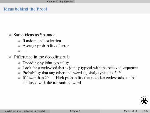
Same ideas as Shannon
Random code selection
Average probability of error
. . .
Difference in the decoding rule
Decoding by joint typicality
Look for a codeword that is jointly typical with the received sequence
Probability that any other codeword is jointly typical is 2−nI
If fewer than 2nI → High probability that no other codewords can be
confused with the transmitted word
[email protected] (Linköping University) Chapter 7 May 3, 2013 7 / 39

Channel Coding Theorem
Proof
Generate a (2nR, n) code at random, independently, according to the
distribution
p(xn) =
n∏
i=1
p(xi). (1)
Codebook (C), contains 2nR codewords as rows of matrix:
C =
x1(1) x2(1) . . . xn(1)...
.... . .
...
x1(2nR) x2(2
nR) . . . xn(2nR)
. (2)
Each entry in the matrix is generated i.i.d, i.e.,
Pr(C) =2nR∏
ω=1
n∏
i=1
p(xi(ω)). (3)
[email protected] (Linköping University) Chapter 7 May 3, 2013 8 / 39
Channel Coding Theorem
Proof
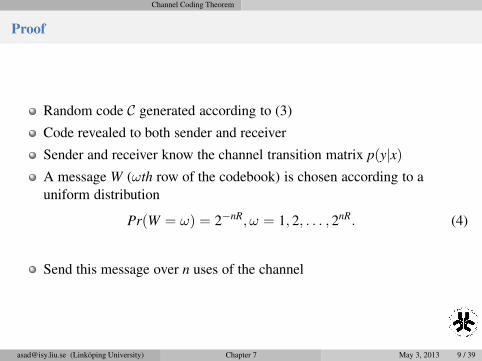
Random code C generated according to (3)
Code revealed to both sender and receiver
Sender and receiver know the channel transition matrix p(y|x)
A message W (ωth row of the codebook) is chosen according to a
uniform distribution
Pr(W = ω) = 2−nR, ω = 1, 2, . . . , 2nR. (4)
Send this message over n uses of the channel
[email protected] (Linköping University) Chapter 7 May 3, 2013 9 / 39
Channel Coding Theorem
Proof
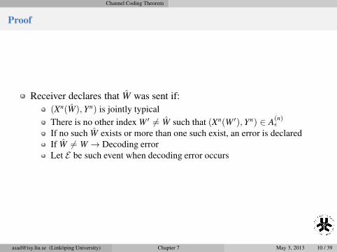
Receiver declares that W was sent if:
(Xn(W), Yn) is jointly typical
There is no other indexW ′ 6= W such that (Xn(W ′), Yn) ∈ A(n)ǫ
If no such W exists or more than one such exist, an error is declared
If W 6= W → Decoding error
Let E be such event when decoding error occurs
[email protected] (Linköping University) Chapter 7 May 3, 2013 10 / 39
Channel Coding Theorem
Probability of Error
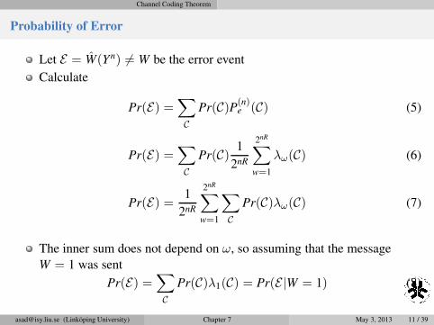
Let E = W(Yn) 6= W be the error event
Calculate
Pr(E) =∑
C
Pr(C)P(n)e (C) (5)
Pr(E) =∑
C
Pr(C)1
2nR
2nR∑
w=1
λω(C) (6)
Pr(E) =1
2nR
2nR∑
w=1
∑
C
Pr(C)λω(C) (7)
The inner sum does not depend on ω, so assuming that the message
W = 1 was sent
Pr(E) =∑
C
Pr(C)λ1(C) = Pr(E|W = 1) (8)
[email protected] (Linköping University) Chapter 7 May 3, 2013 11 / 39
Channel Coding Theorem
Probability of Error
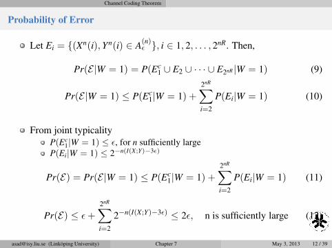
Let Ei = {(Xn(i),Yn(i) ∈ A(n)ǫ }, i ∈ 1, 2, . . . , 2nR. Then,
Pr(E|W = 1) = P(Ec1 ∪ E2 ∪ · · · ∪ E2nR |W = 1) (9)
Pr(E|W = 1) ≤ P(Ec1|W = 1) +
2nR∑
i=2
P(Ei|W = 1) (10)
From joint typicality
P(Ec1|W = 1) ≤ ǫ, for n sufficiently large
P(Ei|W = 1) ≤ 2−n(I(X;Y)−3ǫ)
Pr(E) = Pr(E|W = 1) ≤ P(Ec1|W = 1) +
2nR∑
i=2
P(Ei|W = 1) (11)
Pr(E) ≤ ǫ+
2nR∑
i=2
2−n(I(X;Y)−3ǫ) ≤ 2ǫ, n is sufficiently large (12)
[email protected] (Linköping University) Chapter 7 May 3, 2013 12 / 39
Channel Coding Theorem
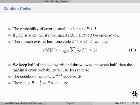
Random Codes
The probability of error is small, as long as R < I
If p(x) is such that it maximized I(X;Y), R < I becomes R < C
There much exist at least one code C∗ for which we have
P(E|C∗) =1
2nR
∑
i
λi(C∗) ≤ 2ǫ (13)
We keep half of the codewords and throw away the worst half, then the
maximal error probability will be less than 4ǫ
The codebook has now 2nR−1 codewords
The rate is R− 1n= R as n → ∞
[email protected] (Linköping University) Chapter 7 May 3, 2013 13 / 39

Channel Coding Theorem
Channel Coding Theorem – Summary
Random coding used as a proof for the theorem
Joint typicality used as a decoding rule
Theorem shows that good codes exist with arbitrarily small error
probability
Does not provide a way of constructing the best codes
If code generated at random with appropriate distribution, the code is
likely to be good but difficult to decode
Hamming codes → simplest of a class of error correcting codes
Turbo codes → Close to achieving capacity for Gaussian channels
[email protected] (Linköping University) Chapter 7 May 3, 2013 14 / 39
Zero-Error Codes
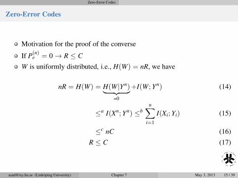
Zero-Error Codes
Motivation for the proof of the converse
If P(n)e = 0 → R ≤ C
W is uniformly distributed, i.e., H(W) = nR, we have
nR = H(W) = H(W|Yn)︸ ︷︷ ︸
=0
+I(W;Yn) (14)
≤a I(Xn;Yn) ≤b
n∑
i=1
I(Xi;Yi) (15)
≤c nC (16)
R ≤ C (17)
[email protected] (Linköping University) Chapter 7 May 3, 2013 15 / 39
Converse to the Channel Coding Theorem
Fano’s Inequality and the Coverse to the Coding Theorem
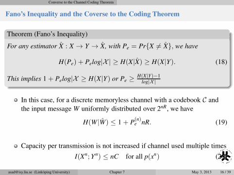
Theorem (Fano’s Inequality)
For any estimator X : X → Y → X, with Pe = Pr{X 6= X}, we have
H(Pe) + Pelog|X | ≥ H(X|X) ≥ H(X|Y). (18)
This implies 1+ Pelog|X ≥ H(X|Y) or Pe ≥H(X|Y)−1
log|X |
In this case, for a discrete memoryless channel with a codebook C and
the input message W uniformly distributed over 2nR, we have
H(W|W) ≤ 1+ P(n)e nR. (19)
Capacity per transmission is not increased if channel used multiple times
I(Xn;Yn) ≤ nC for all p(xn) (20)
[email protected] (Linköping University) Chapter 7 May 3, 2013 16 / 39
Converse to the Channel Coding Theorem
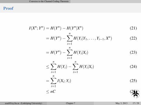
Proof
I(Xn;Yn) = H(Yn)− H(Yn|Xn) (21)
= H(Yn)−n∑
i=1
H(Yi|Y1, . . . ,Yi−1,Xn) (22)
= H(Yn)−n∑
i=1
H(Yi|Xi) (23)
≤n∑
i=1
H(Yi)−n∑
i=1
H(Yi|Xi) (24)
=n∑
i=1
I(Xi;Yi) (25)
≤ nC (26)
[email protected] (Linköping University) Chapter 7 May 3, 2013 17 / 39

Converse to the Channel Coding Theorem
The Proof of Converse
We have W → Xn(W) → Yn → W
For each n, let W is uniformly distributed and
Pr(W 6= W) = P(n)e = 1
2nR
∑
i λi
Using the results we have
nR =a H(W) (27)
=b H(W|W) + I(W; W) (28)
≤c 1+ P(n)e nR+ I(W; W) (29)
≤d 1+ P(n)e nR+ I(Xn;Yn) (30)
≤e 1+ P(n)e nR+ nC (31)
R ≤ P(n)e R+
1
n+ C (32)
[email protected] (Linköping University) Chapter 7 May 3, 2013 18 / 39
Converse to the Channel Coding Theorem
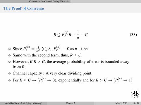
The Proof of Converse
R ≤ P(n)e R+
1
n+ C (33)
Since P(n)e = 1
2nR
∑
i λi, P(n)e → 0 as n → ∞
Same with the second term, thus, R ≤ C
However, if R > C, the average probability of error is bounded away
from 0
Channel capacity : A very clear dividing point.
For R ≤ C → (P(n)e → 0), exponentially and for R > C → (P
(n)e → 1)
[email protected] (Linköping University) Chapter 7 May 3, 2013 19 / 39
Coding Schemes
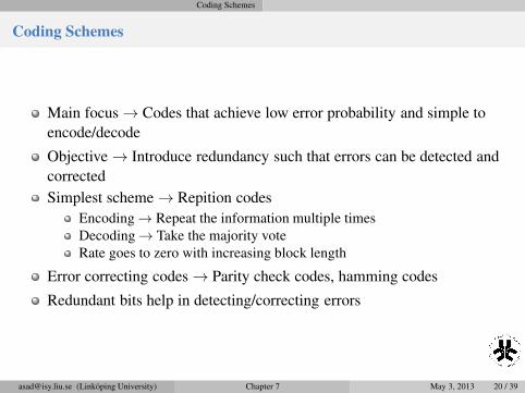
Coding Schemes
Main focus → Codes that achieve low error probability and simple to
encode/decode
Objective → Introduce redundancy such that errors can be detected and
corrected
Simplest scheme → Repition codes
Encoding→ Repeat the information multiple times
Decoding→ Take the majority vote
Rate goes to zero with increasing block length
Error correcting codes → Parity check codes, hamming codes
Redundant bits help in detecting/correcting errors
[email protected] (Linköping University) Chapter 7 May 3, 2013 20 / 39
Coding Schemes
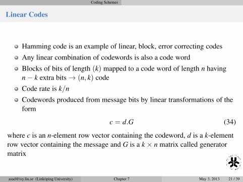
Linear Codes
Hamming code is an example of linear, block, error correcting codes
Any linear combination of codewords is also a code word
Blocks of bits of length (k) mapped to a code word of length n having
n− k extra bits → (n, k) code
Code rate is k/n
Codewords produced from message bits by linear transformations of the
form
c = d.G (34)
where c is an n-element row vector containing the codeword, d is a k-element
row vector containing the message and G is a k × n matrix called generator
matrix
[email protected] (Linköping University) Chapter 7 May 3, 2013 21 / 39

Coding Schemes
Linear Codes
Generator matrix is given by
Gk×n =[Ik×k|Ak×(n−k)
](35)
There is another matrix called parity check matrix H
Rows of H are parity checks on the codewords and should satisfy
cHT = 0 (36)
Can also be derived from G
H =[− PT |In−k
](37)
Should satisfy
GHT = 0 (38)
[email protected] (Linköping University) Chapter 7 May 3, 2013 22 / 39
Coding Schemes
Systematic Linear Codes
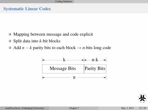
Mapping between message and code explicit
Split data into k-bit blocks
Add n− k parity bits to each block → n-bits long code
Parity BitsMessage Bits
k
n
n-k
[email protected] (Linköping University) Chapter 7 May 3, 2013 23 / 39
Coding Schemes
Hamming Codes
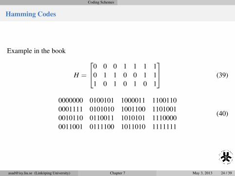
Example in the book
H =
0 0 0 1 1 1 1
0 1 1 0 0 1 1
1 0 1 0 1 0 1
(39)
0000000 0100101 1000011 1100110
0001111 0101010 1001100 1101001
0010110 0110011 1010101 1110000
0011001 0111100 1011010 1111111
(40)
[email protected] (Linköping University) Chapter 7 May 3, 2013 24 / 39
Coding Schemes
Hamming Codes
Formally specified as (n, k, d) codes where d is the distance
Detects and correct up to one bit error
Block Length : n = 2n−k − 1
Number of message bits : k = 2n−k − (n− k)− 1
Distance (min. number of places two codewords differ) : d = 3
Perfect codes → Achieve highest possible rate
[email protected] (Linköping University) Chapter 7 May 3, 2013 25 / 39
Coding Schemes
Decoding of hamming codes
Minimum distance is 3
If codeword c is corrupted in only one place, it will be closer to c
How to discover the closest codeword without searching over all the
codewords
Let ei be a vector with a 1 in the ith position
If codeword corrupt at i, then received vector can be written can be
written as r = c+ ei.
Hr = H(c+ ei) = Hc+ Hei = Hei (41)
Hei is the vector corresponding to the ith column of H.
Hr provides information which bit was corrupted and reversing it to get
the correct codeword
[email protected] (Linköping University) Chapter 7 May 3, 2013 26 / 39
Coding Schemes
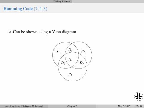
Hamming Code (7, 4, 3)
Can be shown using a Venn diagram
P1 P2
P3
D4
D1
D3D2
[email protected] (Linköping University) Chapter 7 May 3, 2013 27 / 39

Coding Schemes
Hamming Code (7, 4, 3)
Let the message be 11012
11
1
0
[email protected] (Linköping University) Chapter 7 May 3, 2013 27 / 39
Coding Schemes
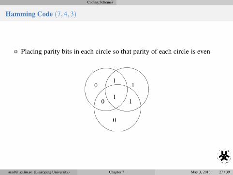
Hamming Code (7, 4, 3)
Placing parity bits in each circle so that parity of each circle is even
11
1
0
0 1
0
[email protected] (Linköping University) Chapter 7 May 3, 2013 27 / 39
Coding Schemes
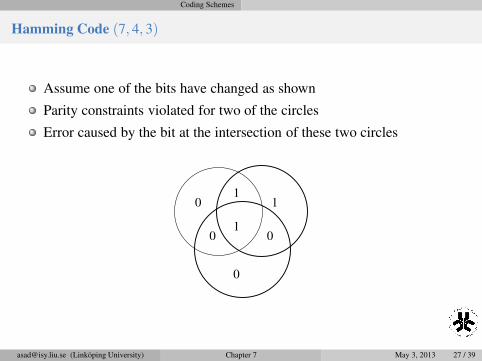
Hamming Code (7, 4, 3)
Assume one of the bits have changed as shown
Parity constraints violated for two of the circles
Error caused by the bit at the intersection of these two circles
01
1
0
0 1
0
[email protected] (Linköping University) Chapter 7 May 3, 2013 27 / 39
Coding Schemes
Other Codes
With large block lengths, more than one error possible
Multi-bit error correcting codes proposed
Reed and Solomon (1959) codes for nonbinary channelsBCH codes, which generalizes Hamming codes using Galois field theory
to construct t-error correcting codes
Examples : cd-players use error correction circuitry based on two
interleaved (32, 28, 5) and (28, 24, 5) Read-Solomon codes that allow the
decoder to correct bursts up to 4000 errors
Convolution Codes→Each output block depends on both the current input
block and some of past input blocks
LDPC and Turbo codes→ Achieving capacity with high probability
[email protected] (Linköping University) Chapter 7 May 3, 2013 28 / 39
Feedback Capacity
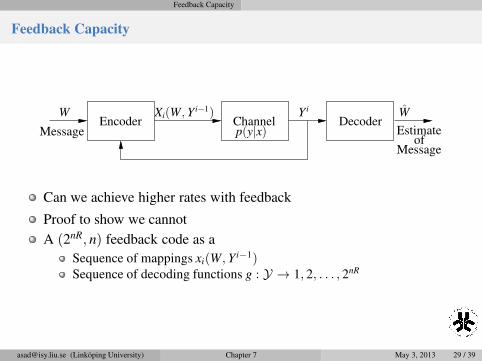
Feedback Capacity
Encoder DecoderChannelEstimate
ofMessage
Message
W Xi(W, Y i−1) Y i W
p(y|x)
Can we achieve higher rates with feedback
Proof to show we cannot
A (2nR, n) feedback code as a
Sequence of mappings xi(W, Y i−1)Sequence of decoding functions g : Y → 1, 2, . . . , 2nR
[email protected] (Linköping University) Chapter 7 May 3, 2013 29 / 39

Feedback Capacity
Feedback Capacity
Definition
The capacity with feedback, CFB, of a discrete memoryless channel is the
supremum of all rates achievable by feedback codes
Theorem (Feedback capacity)
CFB = C = maxp(x)
I(X;Y) (42)
Nonfeedback code is considered as a special case of feedback code, thus
CFB ≥ C (43)
[email protected] (Linköping University) Chapter 7 May 3, 2013 30 / 39
Feedback Capacity
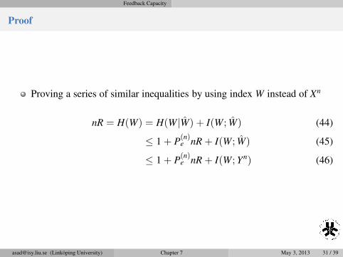
Proof
Proving a series of similar inequalities by using index W instead of Xn
nR = H(W) = H(W|W) + I(W; W) (44)
≤ 1+ P(n)e nR + I(W; W) (45)
≤ 1+ P(n)e nR + I(W;Yn) (46)
[email protected] (Linköping University) Chapter 7 May 3, 2013 31 / 39
Feedback Capacity
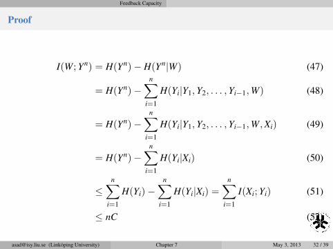
Proof
I(W;Yn) = H(Yn)− H(Yn|W) (47)
= H(Yn)−n∑
i=1
H(Yi|Y1,Y2, . . . ,Yi−1,W) (48)
= H(Yn)−n∑
i=1
H(Yi|Y1,Y2, . . . ,Yi−1,W,Xi) (49)
= H(Yn)−n∑
i=1
H(Yi|Xi) (50)
≤n∑
i=1
H(Yi)−n∑
i=1
H(Yi|Xi) =n∑
i=1
I(Xi;Yi) (51)
≤ nC (52)
[email protected] (Linköping University) Chapter 7 May 3, 2013 32 / 39
Feedback Capacity
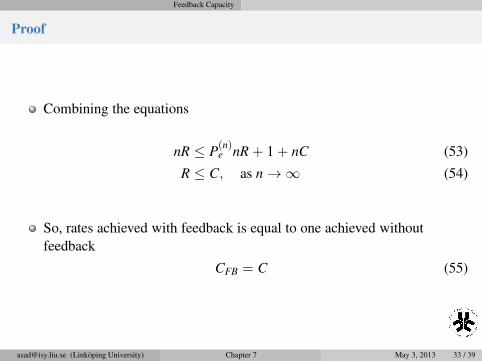
Proof
Combining the equations
nR ≤ P(n)e nR + 1+ nC (53)
R ≤ C, as n → ∞ (54)
So, rates achieved with feedback is equal to one achieved without
feedback
CFB = C (55)
[email protected] (Linköping University) Chapter 7 May 3, 2013 33 / 39
Source-Channel Separation Theorem
Source-Channel Separation Theorem
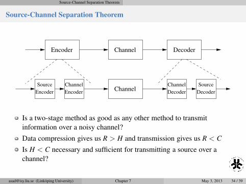
Encoder DecoderChannel
ChannelSource
Encoder Encoder
Channel Channel
Decoder
Source
Decoder
Is a two-stage method as good as any other method to transmit
information over a noisy channel?
Data compression gives us R > H and transmission gives us R < C
Is H < C necessary and sufficient for transmitting a source over a
channel?
[email protected] (Linköping University) Chapter 7 May 3, 2013 34 / 39

Source-Channel Separation Theorem
Source-Channel Separation Theorem
Theorem
If
V1,V2, . . . ,Vn is a finite alphabet stochastic process that satisfies AEP
H(V) < C
there exists a source-channel code with Pr(Vn 6= Vn) → 0
In converse
Theorem
For any staionary stochastic process, if
H(V) > C
the probability of error is bounded away from zero
[email protected] (Linköping University) Chapter 7 May 3, 2013 35 / 39
Source-Channel Separation Theorem
Proof of Theorem
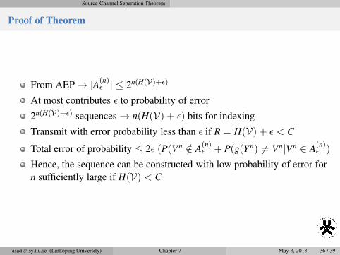
From AEP→ |A(n)ǫ | ≤ 2n(H(V)+ǫ)
At most contributes ǫ to probability of error
2n(H(V)+ǫ) sequences → n(H(V) + ǫ) bits for indexing
Transmit with error probability less than ǫ if R = H(V) + ǫ < C
Total error of probability ≤ 2ǫ (P(Vn /∈ A(n)ǫ + P(g(Yn) 6= Vn|Vn ∈ A
(n)ǫ )
Hence, the sequence can be constructed with low probability of error for
n sufficiently large if H(V) < C
[email protected] (Linköping University) Chapter 7 May 3, 2013 36 / 39
Source-Channel Separation Theorem
Proof of Theorem – Converse
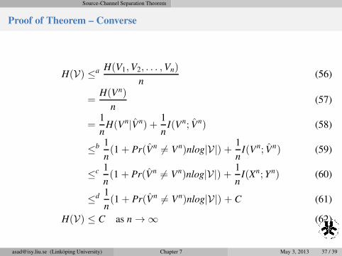
H(V) ≤a H(V1,V2, . . . ,Vn)
n(56)
=H(Vn)
n(57)
=1
nH(Vn|Vn) +
1
nI(Vn; Vn) (58)
≤b 1
n(1+ Pr(Vn 6= Vn)nlog|V|) +
1
nI(Vn; Vn) (59)
≤c 1
n(1+ Pr(Vn 6= Vn)nlog|V|) +
1
nI(Xn;Yn) (60)
≤d 1
n(1+ Pr(Vn 6= Vn)nlog|V|) + C (61)
H(V) ≤ C as n → ∞ (62)
[email protected] (Linköping University) Chapter 7 May 3, 2013 37 / 39
Source-Channel Separation Theorem
Summary of Theorem
Data compression and transmission tied together
Data compression → Consequence of AEP→ There exists a small
subset (|2nH |) of all possible source sequences that contain most of the
probability and that we can therefore represent the source with a small
probability error using H bits per symbol
Data transmission → Based on the joint AEP→ For long block lengths,
the output sequence of the channel is very likely to be jointly typical with
the input codeword, while any other codeword is jointly typical with
probability ≈ 2−nI . Hence we can use about 2nI codewords and still have
negligible error probability.
This theorem shows that we can design the source and channel code
separately and combine the results to achieve optimal performance
[email protected] (Linköping University) Chapter 7 May 3, 2013 38 / 39
