dspace.univ-km.dzdspace.univ-km.dz/jspui/bitstream/123456789/2463/1/thesis.pdfining university of...
TRANSCRIPT
UNIVERSITY OF DJILLALI BOUNAAMA – KHEMIS MILIANA
IMPLEMENTATION AND EVALUATION OF A FREQUENT SUBGRAPH
MINING ALGORITHM WITH HADOOP
AN ITERATIVE MAPREDUCE BASED METHOD
A THESIS
SUBMITTED TO THE COMPUTER SCIENCE DEPARTMENT
FACULTY OF SCIENCE AND TECHNOLOGY - KHEMIS MILIANA UNIVERSITY
IN PARTIAL FULFILLMENT OF THE REQUIREMENTS FOR THE DEGREE OF
MASTER IN COMPUTER SCIENCE
AUTHORS: SUPERVISOR:
ABDELKADER RALEM AHMED PROF. O.HARBOUCHE
ABDELLATIF BOUBEKEUR
JURY MEMBERS:
PRESIDENT: PROF. S. HADJ SADOK.
EXAMINERS: PROF. N. AZZOUZA.
PROF. R. MEGHATRIA.
JUNE 2017-2018

ii
Abstract
Frequent subgraph mining (FSM) is an important task for exploratory data
analysis on graph data. Over the years, many algorithms have been proposed to
solve this task. These algorithms assume that the data structure of the mining
task is small enough to fit in the main memory of a computer. However, as the
real-world graph data grows, both in size and quantity, such an assumption does
not hold any longer. To overcome this, some graph database-centric methods have
been proposed in recent years for solving FSM; however, a distributed solution
using MapReduce paradigm has not been explored extensively. Since, MapReduce
is becoming the de-facto paradigm for computation on massive data, an efficient
FSM algorithm on this paradigm is of huge demand. In this work we study
frequent subgraph mining algorithm called FSM-H which uses an iterative
MapReduce based framework. FSM-H is complete as it returns all the frequent
subgraphs for a given user-defined support, and it is efficient as it applies all the
optimizations that the latest FSM algorithms adopt, our experiments of with real
life and large synthetic datasets validate the effectiveness of FSM-H for mining
frequent subgraphs from large graph datasets.

iii
Résumé:
La fouille des sous graphes fréquent est une tâche importante lorsqu’il s’agit
de l’analyse exploratoire des données de graphe. Au cours des années, de
nombreux algorithmes ont été proposés pour résoudre cette tâche. Ces algorithmes
supposent que la structure de données sujet de l’exploration est petite et peut tenir
dans la mémoire principale d'un ordinateur, cependant, à mesure que les données
du graphe qu’on trouvent dans la vie réelle augmentent, en taille et en
quantité,une telle hypothèse ne tient plus, Pour surmonter ce probléme, ces
dernières années certaines méthodes centrées sur les bases de données du graphe
ont été proposées pour résoudre la fouille des sous-graphe fréquent (FSF),
Cependant, une solution distribuée utilisant le paradigme MapReduce n'a pas été
largement explorée. Ces derniéres années le modèle de programmation
MapReduce est devenu la norme lorsque il s’agit de l’exploration des données
massives,donc une solution basé sur ce paradigme est très aprécié.Dans ce travail
nous étudions une méthode pour la fouille des sous graphe fréquent qui adopte
une approche itérative basé sur le modèle Map Reduce qui s’appelle FSM-H.cet
algorithme est complet puisque il retourne tous les sous graphes fréquents qui ont
un minimum support donnée par l »utilisateur, de plus cet algorithme est efficace
car il applique toutes les optimisations qui sont adoptés par les algorithmes de
fouille de graphes. Nos expériences et tests sur des données de graphe de la vie
réelle et des données synthétiques valident l’efficacité de FSM-H pour la fouille
des sous graphes fréquents dans un ensemble de données massives.

iv
Acknowledgments
There are no words to express our gratitude to Prof.
O.HARBOUCHE, our adviser who helped us to
improve nearly every aspect of this current work,
The study presented in this thesis would not have
happened without his support, guidance, and
encouragement.
It was an honor to have Prof. S.HADJ SADOK,
Prof. N.AZZOUZA, and Prof. R.MEGHATRIA as
committee members for examining this work.
Special thanks are directed to Dr.N.BELKHIER for
having hosted us at the FIMA Lab and allowed us to
work in comfortable conditions.
We would also like to thank our families, they were
always supporting and encouraging us with their
best wishes.

v
CONTENTS Abstract................................................................................................................... ii
Acknowledgments ................................................................................................iv
List of Figures ........................................................................................................ x
List of Tables ...................................................................................................... xiv
Introduction:........................................................................................................... 1
I. Chapter 01 Big Data Principles and techniques ........................................ 5
I.1 Brief History: ............................................................................................. 5
I.2 Definition: .................................................................................................. 6
I.3 Big Data 3V’s : ........................................................................................... 7
I.4 32 Vs Definition and Big Data VENN DIAGRAM: ................................... 9
I.5 Data Types: .............................................................................................. 10
I.5.1 Structured Data: ............................................................................... 11
I.5.2 Unstructured Data: ........................................................................... 12
I.5.3 Structured vs. Unstructured Data: What’s the Difference? ............ 13
I.5.4 Semi-Structured Data: ...................................................................... 14
I.5.5 Quasi-Structured Data: .................................................................... 15
I.6 Data at Rest and Data in Motion: ........................................................... 16
I.6.1 Data at Rest: ..................................................................................... 16
I.6.2 Data in motion:.................................................................................. 17
I.6.3 Data at Rest vs. Data in Motion: ...................................................... 18
I.7 Functional and infrastructure requirements: ........................................ 18
I.8 Data characteristics: ................................................................................ 19
I.9 Big data Challenges: ................................................................................ 20
I.9.1 Data Challenges: ............................................................................... 20
I.9.2 Processing Challenges: ..................................................................... 21
I.9.3 Management Challenges: ................................................................. 21
I.10 Big Data Technology Stack: .................................................................. 22
I.10.1 Layer 1 - Redundant Physical Infrastructure: ............................... 23
I.10.2 Layer 2 – Security Infrastructure: ................................................. 24
I.10.3 Interfaces and Feeds to and from Applications and the ................ 25
Internet (API’s): ......................................................................................... 25
I.10.4 Layer 3 – Operational Databases: .................................................. 25
I.10.5 Layer 4 – Organizing Data Services and Tools: ............................. 31
I.10.6 Layer 5 – Analytical Data Warehouses and Data marts: ............. 32

vi
I.10.7 Layer 6 – Analytics (Traditional and Advanced): .......................... 35
I.10.8 Layer 7 – Reporting and Visualization: ......................................... 38
I.10.9 Layer 8 – Big Data Applications: ................................................... 39
I.11 Virtualization and Cloud Computing in Big Data: .............................. 39
I.11.1 Virtualization: ................................................................................. 40
I.11.2 Cloud Computing: ........................................................................... 42
II. Chapter 02 : Graph Theory and Frequent Subgraph Mining .............. 48
Context: ......................................................................................................... 48
II.1 Data mining: ........................................................................................... 48
II.2 Graph mining: ........................................................................................ 50
II.3 Graphs applications: .............................................................................. 51
II.4 What is Involved in graph mining: ........................................................ 55
II.5 Frequent subgraph mining (FSM): ........................................................ 55
II.6 Graph theory: ......................................................................................... 55
II.7 Preliminary definitions: ......................................................................... 56
II.7.1 Types of graphs: ............................................................................... 56
II.7.2 Subgraph: ......................................................................................... 61
II.7.3 Graph isomorphism: ........................................................................ 62
II.7.4 Automorphism: ................................................................................ 64
II.7.5 Lattice: ............................................................................................. 64
II.7.6 Density: ............................................................................................ 65
II.7.7 Trees: ................................................................................................ 65
II.8 Overview of FSM: ................................................................................... 66
II.9 Formalism:.............................................................................................. 68
II.10 Graph isomorphism detection: ............................................................. 69
II.11 Search strategy:.................................................................................... 70
II.12 FSM algorithmic approaches: .............................................................. 71
II.12.1 Apriori Property: ............................................................................ 71
II.12.2 Apriori based approach: ................................................................ 72
II.12.3 Pattern Growth Approach: ............................................................ 73
II.13 Basic Framework of FSM algorithms:................................................. 75
II.13.1 Canonical Representations:........................................................... 76
II.13.2 Candidate Generation: .................................................................. 79
II.13.3 Support Computing: ...................................................................... 81
II.14 Frequent subgraph mining algorithms: .............................................. 81
II.14.1 Classification based on algorithmic approaches: ......................... 82

vii
II.14.2 Classification based on Search strategy: ...................................... 84
II.14.3 Classification based on the nature of input: ................................. 85
II.14.4 Classification based on the completeness of the output: ............. 85
II.15 Inexact FSM: ........................................................................................ 87
II.16 Exact FSM: ........................................................................................... 88
II.17 Discussion: ............................................................................................ 90
III. Chapter 03 : Hadoop and MapReduce ..................................................... 94
Context: ......................................................................................................... 94
III.1 Presentation of Apache Hadoop: .......................................................... 94
III.2 The motivation for Hadoop: .................................................................. 95
III.3 History of Apache Hadoop: ................................................................... 96
III.4 Hadoop Components and Ecosystem: .................................................. 97
III.4.1 Apache HBase: ............................................................................... 98
III.4.2 Apache Hive:................................................................................... 98
III.4.3 Apache Pig: ..................................................................................... 99
III.4.4 Apache Sqoop : ............................................................................... 99
III.4.5 Apache Flume : ............................................................................. 100
III.4.6 Apache Oozie : .............................................................................. 100
III.4.7 Apache ZooKeeper : ...................................................................... 100
III.4.8 Apache Spark: .............................................................................. 100
III.4.9 Apache Ambari: ............................................................................ 101
III.5 Understanding the Hadoop Distributed ............................................ 101
File System (HDFS): ................................................................................... 101
III.5.1 HDFS Architecture: ..................................................................... 102
III.5.2 Role of Namenode and DataNode in HDFS Architecture: ......... 103
III.5.3 How NameNodes works: .............................................................. 104
III.5.4 How DataNodes Works: ............................................................... 104
III.5.5 Rack Organization: ...................................................................... 106
III.5.6 How Data is stored in HDFS : ..................................................... 106
III.5.7 Data Reading Process in HDFS: .................................................. 108
III.5.8 Data writing Process in HDFS: ................................................... 109
III.5.9 Limitations of HDFS: ................................................................... 111
III.6 MapReduce: ......................................................................................... 112
III.6.1 MapReduce Functional Concept: ................................................. 113
III.6.2 Characteristics of MapReduce: .................................................... 113
III.6.3 The working process of MapReduce: ........................................... 114

viii
III.6.4 Limitations of MapReduce: .......................................................... 115
III.7 YARN (Yet Another Resource Negotiator) : ...................................... 116
III.7.1 YARN architecture: ...................................................................... 117
III.7.2 Advantages of YARN:................................................................... 119
III.8 Commercial distribution of Hadoop: .................................................. 120
III.8.1 Cloudera's Distribution with Hadoop (CDH): .............................. 121
IV. Chapter 04 Implementation ..................................................................... 127
Context: ....................................................................................................... 127
IV.1 Background: ........................................................................................ 127
IV.2 Graph Partitions: ................................................................................ 128
IV.3 Challenges: .......................................................................................... 129
IV.4 Contribution and Goals: ...................................................................... 129
IV.5 Method: ................................................................................................ 130
IV.5.1 Candidate Generation: ................................................................. 132
IV.5.2 Isomorphism checking: ................................................................. 134
IV.5.3 Support Counting: ........................................................................ 135
IV.6 Distributed paradigm of FSM-H: ....................................................... 136
IV.6.1 Pseudo code for the mapper: ........................................................ 137
IV.6.2 Pseudo code for the reducer: ........................................................ 138
IV.7 Execution flow of FSM-H: ................................................................... 138
IV.8 Framework of FSM-H: ........................................................................ 139
IV.8.1 Data partition Phase: ................................................................... 140
IV.8.2 Preparation Phase: ....................................................................... 141
IV.8.3 Mining Phase: ............................................................................... 144
IV.9 Hadoop Pseudo Code: .......................................................................... 145
IV.10 Implementation Details: ................................................................... 147
IV.10.1 Map reduce job configuration: .................................................... 147
V. Chapter 05: Experiments and Results ...................................................... 151
V.1 Experiments: ......................................................................................... 151
V.2 Experimental setup: ............................................................................. 151
V.2.1 Datasets: ......................................................................................... 151
V.2.2 Implementation platform: ............................................................. 155
V.3 Tests and Evaluations: ......................................................................... 155
V.3.1 Runtime of FSM-H for different minimum support: .................... 155
V.3.2 Runtime of FSM-H for varying number of Reducers:................... 157
V.3.3 Runtime of FSM-H on varying number of data nodes: ................ 158

ix
V.3.4 Effect of partition scheme on runtime: ......................................... 159
VI. Conclusion: ................................................................................................... 162
VII. References: .................................................................................................. 164
VIII. Appendices: ............................................................................................... 173

x
List of Figures
Figure I-1 : A short history of big data. --------------------------------------------------------- 6
Figure I-2 : What’s driving the data deluge.(5) ----------------------------------------------- 8
Figure I-3 : From 3Vs, 4Vs, 5Vs, and 6Vs big data definition. -------------------------- 9
Figure I-4 : 32 Vs Venn diagrams hierarchical model. ----------------------------------- 10
Figure I-5 : Big data growth is increasingly unstructured. ----------------------------- 11
Figure I-6 : Example of structured data. ----------------------------------------------------- 11
Figure I-7 : Example of unstructured data : Video about Antarctica expedition. 13
Figure I-8 : Excerpt from semi-structured data JSON File. ---------------------------- 15
Figure I-9 : Example of Click Stream Data , EMC data science website search
results. --------------------------------------------------------------------------------------------------- 16
Figure I-10 : Workload requirements (Data at rest vs Data in motion). ----------- 18
Figure I-11 : The cycle of Big data Management. ------------------------------------------ 19
Figure I-12 : Big Data Challenges. ------------------------------------------------------------- 22
Figure I-13 : Big Data technology stack.(7) -------------------------------------------------- 23
Figure I-14 : A document can have many types of values : scalar , lists and
nested documents. ----------------------------------------------------------------------------------- 28
Figure I-15 : Columnar data store -------------------------------------------------------------- 29
Figure I-16 : Key/Value data store ------------------------------------------------------------- 30
Figure I-17 : Graph data store ------------------------------------------------------------------- 31
Figure I-18 : OLAP Cube Sales Data Example. -------------------------------------------- 34
Figure I-19 : Data Warehouse Component. -------------------------------------------------- 35
Figure I-20 : Categories of Data Analytics Techniques. --------------------------------- 36
Figure I-21 : Partitioning – Isolation – Encapsulation. ---------------------------------- 40
Figure I-22 : Application Virtualization. ----------------------------------------------------- 41
Figure I-23 : Data Center vs. Cloud Computing.------------------------------------------- 43
Figure I-24 : Cloud Computing Stack. --------------------------------------------------------- 44
Figure II-1: The steps of the KDD process.(14) --------------------------------------------- 49
Figure II-2 : Graph mining Related Concept ------------------------------------------------ 50

xi
Figure II-3 : Graph representation of a chemical compound.(13) --------------------- 52
Figure II-4 : Frequent subgraph mined from a variety of chemical compounds - 52
Figure II-5 : Protein – Protein interaction network. -------------------------------------- 53
Figure II-6 : Social media graphs : there are complex Groups, links, preferences
and attributes. ---------------------------------------------------------------------------------------- 54
Figure II-7 : Mining graph evolution rules. -------------------------------------------------- 54
Figure II-8 : (a) Simple Graph, (b) nom simple graph having multiple edge (left)
nom simple graph having loops(right). -------------------------------------------------------- 56
Figure II-9 : 3-Regular graph k=3. ------------------------------------------------------------- 57
Figure II-10 : Unlabeled and Labeled graphs. ---------------------------------------------- 57
Figure II-11 : Undirected graph (left), Directed graph (right). ------------------------ 58
Figure II-12 : Two complete and connected graphs with 5 and 3 vertices
respectively when considered together they form a disconnected graph. ---------- 61
Figure II-13 : (a) a graph G , (b), (c) , (d) represent a general, induced, and
connected subgraphs respectively.(15) -------------------------------------------------------- 62
Figure II-14 : Graph isomorphism. ------------------------------------------------------------- 63
Figure II-15 : Subgraph Isomorphism. -------------------------------------------------------- 63
Figure II-16 : Lattice(G). --------------------------------------------------------------------------- 65
Figure II-17 : The distribution of the most significant FSM algorithms with
respect to year of introduction and application domain. -------------------------------- 67
Figure II-18 : DFS and BFS search strategies. --------------------------------------------- 71
Figure II-19 : Apriori Algorithm. ---------------------------------------------------------------- 72
Figure II-20 : Apriori-based Approach. -------------------------------------------------------- 73
Figure II-21 : PatternGrowth algorithm. ----------------------------------------------------- 74
Figure II-22 : PatternGrowth-based approach. --------------------------------------------- 75
Figure II-23 : Baseline algorithm for FSM. -------------------------------------------------- 76
Figure II-24 : A simple graph G with its corresponding adjacency matrix. ------- 77
Figure II-25 : An illustration of the right most expansion. ----------------------------- 80
Figure II-26 : Classification of FSM Algorithms.(86) ------------------------------------- 86
Figure III-1 : The Hadoop Kernel. -------------------------------------------------------------- 95
Figure III-2 : Brief History of Hadoop. -------------------------------------------------------- 97
xii
Figure III-3 : The Hadoop Ecosystem. -------------------------------------------------------- 101
Figure III-4 : HDFS Architecture. ------------------------------------------------------------- 103
Figure III-5 : How NameNodes Works. ------------------------------------------------------ 104
Figure III-6 : How DataNodes Works. -------------------------------------------------------- 105
Figure III-7 : Rack Organization. -------------------------------------------------------------- 106
Figure III-8 : Data Storage in HDFS. -------------------------------------------------------- 107
Figure III-9 : HDFS Reading Process. -------------------------------------------------------- 108
Figure III-10 : HDFS Writing Process. ------------------------------------------------------- 110
Figure III-11 : How MapReduce Works. ----------------------------------------------------- 113
Figure III-12 : MapReduce Procedure. ------------------------------------------------------- 115
Figure III-13 : YARN Applications. ----------------------------------------------------------- 117
Figure III-14 : Yarn Architecture. ------------------------------------------------------------- 118
Figure III-15 : The Hadoop Ecosystem along with the Commercial Distribution.
------------------------------------------------------------------------------------------------------------ 121
Figure III-16 : CDH Main Admin Console “Cloudera Manager”. -------------------- 122
Figure III-17 : Cloudera Manager Architecture.(90) ------------------------------------- 124
Figure IV-1 : (a) Graph database with 3 graphs with labeled vertices ------------ 128
Figure IV-2 : Iterative MapReduce Algorithm --------------------------------------------- 130
Figure IV-3 : Candidate generation subtree rooted under A-B. ---------------------- 133
Figure IV-4 : Graph isomorphism. ------------------------------------------------------------- 135
Figure IV-5 : Support Counting. --------------------------------------------------------------- 136
Figure IV-6 : Mapper of distributed FSM-H Algorithm. -------------------------------- 137
Figure IV-7 : Reducer of distributed FSM-H Algorithm. ------------------------------- 138
Figure IV-8 : Execution flow of FSM-H Algorithm. -------------------------------------- 139
Figure IV-9 : Framework of FSM-H. ---------------------------------------------------------- 140
Figure IV-10 : Input dataset after partition and filtering phase. -------------------- 141
Figure IV-11 : The static data structures and A-B-C pattern object in partition 1
and 2 (a) Edge-extension-map (b) Edge-OL (c) and (d) A-B-C Pattern object. --- 142
Figure IV-12 : One iteration of the mining phase of FSM-H with respect to
pattern A-B. ------------------------------------------------------------------------------------------- 145
Figure IV-13 : Data partitioning Phase. ----------------------------------------------------- 145

xiii
Figure IV-14 : Preparation Phase. ------------------------------------------------------------- 146
Figure IV-15 : Mining Phase.-------------------------------------------------------------------- 147
Figure V-1 : (a) Exerpt from the yeast graph dataset file. ----------------------------- 153
Figure V-2 : Example of two hydrogen-suppressed molecular graphs depicting
butane and cyclobutane. -------------------------------------------------------------------------- 154
Figure V-3 : Line Plot Showing the relationship between the minimum support
threshold and the running time n minutes for (a) Yeast, (b) SN12C (c) OVCAR-8
(d) NCI-H23 and (e) SF295. ---------------------------------------------------------------------- 156
Figure V-4 : Line Plot showing the relationship between the minimum support
threshold and the running time of Map and Reduce phase of FSM-H in (a)(b)
Yeast and (c)(d) SN12C --------------------------------------------------------------------------- 157
Figure V-5 : Bar Plot showing the relationship between the number of Reducer
and the running time of FSM-H in (a) Yeast (b) OVCAR-8.. -------------------------- 158
Figure V-6 : Relationship between the execution time and the number of data
nodes : (a) Bar plot shows the execution time (b) Line plot shows the speedup
with respect to the execution time using 2 data nodes configuration . ------------ 159
Figure V-7 : Bar plot showing the relationship between the partition count and
the running time of FSM-H for Yeast dataset. -------------------------------------------- 161

xiv
List of Tables
Table I-1 : Structured vs. unstructured data. ........................................................ 14
Table I-2 : Virtualization of different elements. .................................................... 42
Table II-1 : Graph mining research subdomains ................................................... 51
Table II-2 : Categorization of exact matching (sub) graph isomorphism testing
algorithms. .............................................................................................................. 69
Table II-3 : Classification of FSM algorithms based on Apriori based approach. 83
Table II-4 : Classification of FSM algorithms based of Pattern Growth approach.
................................................................................................................................. 83
Table V-1 : statistics of real life graph datasets. ................................................. 152

Introduction

INTRODUCTION
1
Introduction:
We live in the era where almost everything surrounding us is generating some
kind of data, a search on a search engine is being logged, a heartbeat of a patient
in the hospital generates data, the flipping of channels when watching TV is being
captured by cable companies, Data this valuable asset is created constantly, and
at an ever-increasing rate, and so must be stored somewhere for some purpose.
Organizations and institutions have been storing huge volumes of data that is
of various types and in different forms for several years now. the data remained
on backup tapes or drives, and so it could only be used in case of emergency to
retrieve important data, This is changing, Organizations want now to use this data
to get insight to help understand existing problems, seize new opportunities, and
be more profitable, the study and analysis of these volumes of data that have the
unique feature of being “massive, high dimensional, heterogeneous, complex,
unstructured, incomplete, noisy, and erroneous” has given birth to a term called
big data.
It is important to mention that the move to big data is not exclusively driven
just by businesses, Science, Research and Government activities have also helped
to derive it forward, just think about analyzing the human genome, or dealing with
all the astronomical data collected at observatories to advance our understanding
of the world around us, that being said big data find its application in several
different domains ranging from web, computational biology, astronomy,
chemoinformatics, medicine, e-commerce just to name a few, in these domains,
analyzing and mining of massive data for extracting novel insights has become a
routine task, thus giving rise obviously to various basic and advanced data
analytics methods appropriate to the problem in question like data mining , social
network analysis for social websites, discourse-level analysis for text , …. etc.
Data mining for instance is an analytics method which have a basic objective
of discovering hidden and useful data pattern from very large datasets. Graph
mining is a data mining technique that gained much attention in the last few

INTRODUCTION
2
decades as novel approach when it comes to exploratory data analysis for mining datasets
represented by a graph datastructure.
Graphs are common data structures used to represent and model real-world
systems, e.g. social networks, chemical molecules, map of roads in a country.
Frequent sub graph mining which is the subject of this report is considered as a
sub section of graph mining domain which is extensively used to identify
subgraphs in large graph datasets whose occurrences counts are above a specified
minimum support threshold, also used for graph classification, building indices
and graph clustering purposes. The frequent sub graph mining is addressed from
various perspectives and viewed in different directions based upon the domain
expectations.
Mining patterns from graph databases is challenging since graph related
operations, such as subgraph testing, generally have higher time complexity than
the corresponding operations on item sets, sequences, and trees, moreover the
tremendously increasing size of existing graph databases makes the mining even
much harder. hence processing or analyzing such data to get insight efficiently
was very difficult in the past, because traditional methods for analysis and mining
are not designed to handle massive data and complex operation on it, and so do
not withstand the requirements, therefore in recent years, many such methods are
re-designed and re-implemented under a computing framework that is better
equipped to handle big data idiosyncrasies.
Among the recent effort for building a suitable computing platform for
analyzing massive data, the Map Reduce framework of distributed computing has
been the most successful. Because it adopts a data centric approach of distributed
computing with the ideology of “moving computation to data”, besides it uses a
distributed file system that is particularly optimized to improve the IO
performance, while handling massive data, another main reason for this
framework to gain attention of many admirers is the high level of abstraction that
it provides, which keeps many system level details hidden from the programmers
and allow them to concentrate more on the problem specific computational logic.

INTRODUCTION
3
In this report we propose an implementation and a detailed evaluation of a
novel iterative map reduce based frequent subgraph mining algorithm “FSM-H”,
in the Hadoop platform.
The report is organized in five chapters as follows:
In chapter 01, we define big data, and review its evolution in the past 20 years.
we present the underlying technology architecture that support it, as well as
various data analytics methods.
Chapter 02 is divided in two parts:
Part 01 : discusses the Graphs data structure, means of representing them on
machines, Graph theory terminology.
Part 02 : gives the state of the art of frequent subgraph mining approaches, a
survey on different FSM algorithms and their classification with respect to
different considerations, as well as solutions addressing the major issues that one
may encounter when enumerating subgraphs in large datasets.
Chapter 03 covers the internals of the Apache Hadoop ecosystem, the platform
in which the algorithm is implemented, review its features and capabilities, runs
into the technical details of the Hadoop distributed file system HDFS and the
MapReduce programming model.
Chapter 04 present a thorough explanation of the FSM-H algorithm studied,
giving the implementation details, describing for instance the map and the reduce
functions, covering the techniques used for the purpose of carrying out
isomorphism checking, candidate subgraph generation and support counting.
In Chapter 05 we present the experiments and analyses the results, and so
empirically demonstrate the performance of FSM-H on real world chemical
compounds datasets.

4
Chapter I:
Big Data Principles and
Techniques

CHAPTER 01 BIG DATA PRINCIPLES AND TECHNIQUES
5
I. Chapter 01
Big Data Principles and techniques
Context:
The term big data is now well understood for its well-defined characteristics.
more the usage of big data is now looking promising. this chapter being an
introduction draws a comprehensive picture on the history and progress of big
data, it defines the big data characteristics, and then presents the big data
technology stack, a discussion on the state of the art of big data analytics
techniques including data mining is also presented.
I.1 Brief History:
Although the term big data itself is relatively new, when it was first coined by
a Silicon Graphics Inch SGI chief scientist called John Mashey in 1990, the
origins of large data sets go back to the 1960s and '70s when the world of data was
just getting started, with the first data centers and the development of the
relational database.
Around 2005, people began to realize just how much data users generated
through Facebook, YouTube, and other online services. Hadoop an open-source
framework created specifically to store and analyze big data sets was developed
that same year. NoSQL databases also began to gain popularity during that time.
In the years since then, the volume of big data has skyrocketed. Users are still
generating huge amounts of data but it’s not just humans who are doing it.
With the advent of the IoT more objects and devices are connected to the
internet, gathering data on customer usage patterns and product performance.
While big data has come far, its usefulness is only just beginning. Cloud
computing has expanded big data possibilities even further. The cloud offers truly
elastic scalability, where developers can simply spin up ad hoc clusters to test a

CHAPTER 01 BIG DATA PRINCIPLES AND TECHNIQUES
6
subset of data.(1)
Figure I-1 Highlights the most important technical events in the history of big
data:
Figure I-1 : A short history of big data.
I.2 Definition:
Big data is an abstract concept. Apart from masses of data, it also has some
other features, which determine the difference between itself and “massive data”
At present, although the importance of big data has been generally recognized,
when you read articles about big data, it becomes clear that there are varying
definitions of it, this looseness leads to considerable confusion. In general, big data
refers to the datasets that could not be perceived, acquired, managed, and
processed by traditional IT and software/hardware tools within a tolerable time.(2)
Because of different concerns, scientific and technological enterprises, research

CHAPTER 01 BIG DATA PRINCIPLES AND TECHNIQUES
7
scholars, data analysts, and technical practitioners have different definitions of
big data. In 2010, Apache Hadoop defined big data as “datasets which could not be
captured, managed, and processed by general computers within an acceptable
scope.”(3), On the basis of this definition, in May 2011, McKinsey & Company, a
global consulting agency announced Big Data as “the Next Frontier for Innovation,
Competition, and Productivity.”(1)
As a matter of fact, the wider and most used definition of big data, has been
proposed as early as 2001 when Doug Laney, an analyst of META (presently
Gartner) defined challenges and opportunities brought by the increased data in
terms of a 3 Vs attributes.
I.3 Big Data 3V’s :
Volume – This is big data’s most identifiable aspect. It refers to the mind-
boggling amount of data generated each second by users, sensors, and server. just
think of all the emails, Twitter messages, photos, video clips that we produce and
share every second. We are not talking terabytes, but zettabytes or brontobytes of
data. On Facebook alone we send 10 billion messages per day, click the like button
4.5 billion times and upload 350 million new pictures each and every day. If we
take all the data generated in the world between the beginning of time and the
year 2000, it is the same amount we now generate every minute.
Velocity – refers to the speed at which new data is generated and the speed
at which data moves around. This covers everything from emails to real-time
monitoring, to online financial transactions. Consider that more than 100 million
emails are composed every minute, and Just think of social media messages going
viral in minutes. Velocity therefore suggest two kind of analytics batch and real
time.
Variety – refers to the different types of data we can now use. In the past we
focused on structured data that neatly fits into tables or relational databases such
as financial data (for example, sales by product or region). But now Nearly all the
data generated is in an unstructured format, in fact, 80 percent of the world’s data
is now unstructured and therefore can’t easily be put into tables or relational

CHAPTER 01 BIG DATA PRINCIPLES AND TECHNIQUES
8
databases, just think of sensor data or social media posts to get an idea of the
variety of content.(4)
The below figure highlights several sources that drives the big data deluge:
Figure I-2 : What’s driving the data deluge.(5)
Over the years, large enterprises like IBM have expanded the definition to
include five V’s, incorporating:
Veracity – Big Data Veracity refers to the biases, noise and abnormality in
data, this is a highly significant factor that only really became apparent as data
analysts began to work with big data. The trustworthiness of the data source and
the time necessary to clean up the data before it could be used deeply impact how
useful the data is to an enterprise. The length of time between when the data is
collected and the time it is analyzed contributed to a new plague of “data rot.”(2)
Value – As the above suggests, the complexity of converting raw data into
useful insights and actionable conclusions influences whether it should be
considered big data or merely a big headache, the purpose of the value
characteristic is to answer the following question:
“Does the data contain any valuable information for my needs”.

CHAPTER 01 BIG DATA PRINCIPLES AND TECHNIQUES
9
Really, there’s no reason to stop at five. The number of Vs that could be added
continue to increase as more people begin exploring the possibilities. Data experts
have suggested adding vulnerability to stress the growing security concerns over
the use of big data and viability to highlight the fact that not all data, even if
accurate, will have a meaningful impact on desired outcomes.
Figure I-3 shows the progress of big data from 2V’s attributes up to 6V’s.
Figure I-3 : From 3Vs, 4Vs, 5Vs, and 6Vs big data definition.
I.4 32 Vs Definition and Big Data VENN DIAGRAM:
Laney’s 3Vs have captured the importance of Big Data characteristics
reflecting the pace and exploration phenomena of data growth during the last few
years. these 3V’s however represented just a syntactic or logical meaning of Big
Data, therefore for a more precise and semantic meaning the relationship of data,
business intelligence, and statistics have to be included incorporating all
attributes of these three domains, which in fact represent a hierarchical model for

CHAPTER 01 BIG DATA PRINCIPLES AND TECHNIQUES
10
a variety of complex problems and applications.(6)
The Figure below presents a venn diagram showing all logical relations of
Data, BI, Statistics in terms of their 32V’s (9V’s) attributes considered for big data
as follows:
Data Attributes: Volume, Variety, Velocity.
BI Attributes: Visibility, Verdict, Value.
Statistics Attributes: Veracity, Validity, Variability.
This is actually considered as the most accurate definition of big data.
.
Figure I-4 : 32 Vs Venn diagrams hierarchical model.
I.5 Data Types:
Big data can come in multiple forms, including structured and non-structured
data such as financial data, text files, multimedia files, and genetic mappings,

CHAPTER 01 BIG DATA PRINCIPLES AND TECHNIQUES
11
Figure I-5 shows four types of data structures, with 80–90% of future data growth
coming from non-structured data types.
Figure I-5 : Big data growth is increasingly unstructured.
I.5.1 Structured Data:
The term structured data generally refers to data containing a defined data
type, format, and structure, examples of structured data include numbers, dates,
and strings (for example, a customer’s name, address), transaction data, online
analytical processing (OLAP) data cubes, CSV files, and even simple spreadsheets,
this kind of data accounts for about 20 percent of the data that is out there, most
of structured data resides in relational databases (RDBMS). And it is eminently
searchable using a language like structured query language (SQL).
Figure I-6 : Example of structured data.

CHAPTER 01 BIG DATA PRINCIPLES AND TECHNIQUES
12
The sources of structured data are divided into two categories:
Computer or machine-generated: Machine-generated data generally
refers to data that is created by a machine without human intervention.
Human-generated: This is data that humans, in interaction with
computers, supply.
Machine-generated structured data could include the following:
Sensor data: Examples include radio frequency ID (RFID) tags, smart
meters, medical devices, and Global Positioning System (GPS) data.
Web log data: When servers, applications, networks, and so on operate,
they capture all kinds of data about their activity.
Point-of-sale data: When the cashier swipes the bar code of any
product that you are purchasing, all that data associated with the
product is generated.
Examples of structured human-generated data might include the following:
Input data: This is any piece of data that a human might input into a
computer, such as name, age, income, non-free-form survey responses,
and so on.
Gaming-related data: Every move you make in a game can be
recorded.(7)
I.5.2 Unstructured Data:
Data that has no inherent structure, which may include text documents,
PDFs, images, and video. Unstructured data is really most of the data that we may
encounter as it represents 80% of the whole data out there, it may be human or
machine-generated. It may also be stored within a non-relational database. Until
recently, however, the technology didn’t really support doing much with it except
storing it or analyzing it manually.
The term unstructured data is misleading because each document may contain
its own specific internal structure or formatting based on the software that created
it. However, what is internal to the document is truly unstructured.
CHAPTER 01 BIG DATA PRINCIPLES AND TECHNIQUES
13
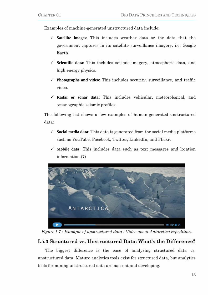
Examples of machine-generated unstructured data include:
Satellite images: This includes weather data or the data that the
government captures in its satellite surveillance imagery, i.e. Google
Earth.
Scientific data: This includes seismic imagery, atmospheric data, and
high energy physics.
Photographs and video: This includes security, surveillance, and traffic
video.
Radar or sonar data: This includes vehicular, meteorological, and
oceanographic seismic profiles.
The following list shows a few examples of human-generated unstructured
data:
Social media data: This data is generated from the social media platforms
such as YouTube, Facebook, Twitter, LinkedIn, and Flickr.
Mobile data: This includes data such as text messages and location
information.(7)
Figure I-7 : Example of unstructured data : Video about Antarctica expedition.
I.5.3 Structured vs. Unstructured Data: What’s the Difference?
The biggest difference is the ease of analyzing structured data vs.
unstructured data. Mature analytics tools exist for structured data, but analytics
tools for mining unstructured data are nascent and developing.

CHAPTER 01 BIG DATA PRINCIPLES AND TECHNIQUES
14
The following table depicts some of their differences:
Table I-1 : Structured vs. unstructured data.
Structured Data Unstructured Data
Characteristics Pre-defined data
models
Usually text only
Easy to search
No pre-defined data
model
May be text, images,
sound, video or other
formats
Difficult to search
Resides in Relational databases
Data Warehouses
Applications
NoSQL databases
Data Warehouses
Data lakes
Generated by Humans or machines Human or machines
Typical
applications
Airplane reservations
systems
Inventory control
CRM systems
ERP systems
Word Processing
Presentation software
Email clients
Tools for viewing or
editing media
I.5.4 Semi-Structured Data:
Semi-structured data is a kind of data that falls between structured and
unstructured data. Semi-structured data does not necessarily conform to a fixed
schema (that is, structure) but may be self-describing and may have simple
label/value pairs. It maintains internal tags and markings that identify separate
data elements, which enables information grouping and hierarchies. Both
documents and databases can be semi-structured. This type of data only
represents about 5-10% of the structured/semi-structured/unstructured data pie,
but has critical business usage cases.

CHAPTER 01 BIG DATA PRINCIPLES AND TECHNIQUES
15
Email is a very common example of a semi-structured data type. Although
more advanced analysis tools are necessary for thread tracking, near-dedupe, and
concept searching; email’s native metadata enables classification and keyword
searching without any additional tools.
Examples of Semi-Structured Data:
Extensible markup language XML: This is a semi-structured document
language, it is a set of document encoding rules that defines a human- and
machine-readable format, XML data files are self-describing, and has a discernible
pattern that enables parsing.
Open standard JavaScript Object Notation JSON: this is another
semi-structured data interchange format.
Figure I-8 : Excerpt from semi-structured data JSON File.
I.5.5 Quasi-Structured Data:
Textual data with erratic data formats that can be formatted with effort, tools,
and time for instance, web clickstream data that may contain inconsistencies in
data values and formats.(5)

CHAPTER 01 BIG DATA PRINCIPLES AND TECHNIQUES
16
Figure I-9 : Example of Click Stream Data , EMC data science website search
results.
I.6 Data at Rest and Data in Motion:
Apart from being classified as structured and unstructured, big data is also
categorized as data at rest and data in motion, each of these categorizes has
different infrastructure requirements.
I.6.1 Data at Rest:
Data at rest refers to the data that is captured at asynchronous intervals, this
data can be stored in hard disk and flash storage, and can be retrieved and
analyzed after the data creating events occurs, let us understand this better with
an example of a retail store:
A retailer uses the analysis of the previous month sales data (data at rest), to
decide marketing strategy and business activities for the present month, using
this data the retailer can decide on the kind of the marketing strategies that will
entice its customers and increases sales, while the data provide value, the business

CHAPTER 01 BIG DATA PRINCIPLES AND TECHNIQUES
17
impact is limited and dependent on the customer coming back to the store to take
advantages of the marketing strategies and activities.(8)
Data at rest is usually managed by batch processing or online transaction
processing methods OTLP (which will be covering later in the chapter), and
therefore does not need an on demand infrastructure, however the infrastructure
must be scalable to support large data sets for both transaction, that is RDBMS
and the analysis which means:
Data warehousing
Business Intelligence
The two latter concepts will be covered in details later when presenting the
big data technology stack.
I.6.2 Data in motion:
Data in motion (real-time data) is the term used for data as it is in transit over
the network, often there is a need to manage and process large volume of data that
is continuously flowing, such data captured at frequent intervals typically from
electronic sensors and devices is called data in motion.
The volume and velocity of such data type will be very high and we need
various tools to process such continuous streams of data.
Picture the scenario of a hospital ICU for example:
In a hospital ICU Electronic devices continuously monitors various medical
parameters of a patient, however there are multiple patients with various medical
conditions in the ICU, considering the criticality of the patient conditions, doctors
need to be alerted if there is a branch in the threshold value of any parameter at
any given point in time, in this scenario there are vast amounts of data in a form
of parameter values flowing continuously into a computer system, such data is a
real-time data, so for alerts to be raised such data need to be processed and
analyzed to check for any breach within small time windows within the computer
memory and when it is flowing, this is done by various big data stream processing
technologies.(8)

CHAPTER 01 BIG DATA PRINCIPLES AND TECHNIQUES
18
I.6.3 Data at Rest vs. Data in Motion:
How is data in motion different from data at rest?
The key difference between the two data sets is at the point of analytics unlike
data at rest data in motion analytics occurs in real time as the event happens and
organizations stand to gain tremendous opportunity to improve business results
in real time from insights gained from streaming data.
The figure below highlights some workload requirements for both data at rest
and data in motion.
Figure I-10 : Workload requirements (Data at rest vs Data in motion).
I.7 Functional and infrastructure requirements:
Before we examine the big data technology stack and its component let first
discuss the different architectural considerations associated with big data. This
architectural foundation must take into account the functional requirements as
well as the infrastructure requirements, these will form the design principles that
are critical for creating a strong environment that is conducive for big data, so
what are those functional requirements.
The architecture design must support the following:
First data is captured, and then organized and integrated, after this phase is
successfully implemented, data can be analyzed then based on the problem being
addressed, finally we act on the results of the analysis, although this sounds
straightforward, certain nuances of these functions are complicated. Validation

CHAPTER 01 BIG DATA PRINCIPLES AND TECHNIQUES
19
when capturing data is particularly an important issue, for instance when
combining data sources, it is critical that we have the ability to validate that these
sources make sense when combined. Also, certain data sources may contain
sensitive information, therefore the implementation of sufficient levels of security
and governance is of high importance.(7)
Figure I-11 : The cycle of Big data Management.
In addition to the functional requirements it is important that the architecture
supports:
High power and high speed computation.
High data storage.
Right redundancy, etc.
I.8 Data characteristics:
As we discuss earlier, big data consists of structured, semi-structured, and
unstructured data. And we often have a lot of it, and it can be quite complex. When
you think about analyzing it, you need to be aware of the potential characteristics
of it:
It can come from untrusted sources: Big data analysis (which will be
covering a bit later in the chapter) often involves aggregating data from various
sources, these may include both internal and external data sources. How
trustworthy are these external sources?
The information may be coming from an unverified source, so the integrity of

CHAPTER 01 BIG DATA PRINCIPLES AND TECHNIQUES
20
this data needs to be considered in the analysis of information.
It can be dirty: Dirty data refers to inaccurate, incomplete, or erroneous
data. This may include the misspelling of words; a sensor that is broken, not
properly calibrated, or corrupted in some way; or even duplicated data, of course,
one might say that the dirty data should be cleaned, but in reality it may contain
interesting outliers so the cleansing strategy will probably depend on the source
and type of data and the goal of your analysis.
The signal-to-noise ratio can be low: In other words, the signal (usable
information) may only be a tiny percent of the data; the noise is the rest. Being
able to extract a tiny signal from noisy data is part of the benefit of big data
analytics.
It can be real-time: In many cases, you’ll be trying to analyze real-time data
streams from social media websites like Facebook or Twitter for instance.(7)
I.9 Big data Challenges:
Big data promises to be transformative, the effective use of this data cannot
only deliver substantial top and bottom line profits but also improve the
performance of existing functions and also create opportunities for growth and
expansion, yet very few organizations are able to reap these benefits, the main
reason being the lack of the right infrastructure to handle big data leading to poor
data management and consequent loss of revenue. one of the challenges that
businesses and organization face while delivering big data capabilities is the
strain that it puts on their existing IT infrastructure due to the huge data influx
and thereby slowing the systems, businesses will need to invest in a more robust
architecture that can handle the size and dynamic nature of big data, but before
looking at the technology architecture supporting big data, let us review some of
the challenges which are primarily divided into three groups, (i) data,
(ii) processing and (iii) management challenges.(9)
I.9.1 Data Challenges:
while dealing with large amounts of information we face such challenges
as volume, variety, velocity and veracity.
CHAPTER 01 BIG DATA PRINCIPLES AND TECHNIQUES
21
Volume: refers to the large amount of data, especially, machine-generated.
This characteristic defines a size of the data set that makes its storage and
analysis problematic utilizing conventional database technology.
Variety: Multiplicity of the various data implied by variety results in the issue
of its handling.
Velocity: the speed of new data generation and distribution requires the
implementation of real-time processing for the streaming data analysis (e.g. on
social media, different types of transactions or trading systems, etc.)
Veracity: refers to the complexity of data which may lead to a lack of quality
and accuracy.
This characteristic reveals several challenges: uncertainty, imprecision,
missing values, misstatement and data availability. There is also a challenge
regarding data discovery that is related to the search of high quality data in data
sets.
I.9.2 Processing Challenges:
The second branch of Big Data challenges is called processing challenges. It
includes data collection, resolving similarities found in different sources,
modification data to a type acceptable for the analysis, the analysis itself and the
output representation, i.e. the results must be visualized in a form that is most
suitable for human perception.(9)
I.9.3 Management Challenges:
The last type of challenges offered by this classification is related to data
management. Management challenges usually refer to secured data storage, its
processing and collection. Here the main focuses of study are: data privacy, its
security, governance and ethical issues. Most of them are controlled based on
policies and rules provided by information security institutes on state or
international levels.(9)

CHAPTER 01 BIG DATA PRINCIPLES AND TECHNIQUES
22
Figure I-12 : Big Data Challenges.
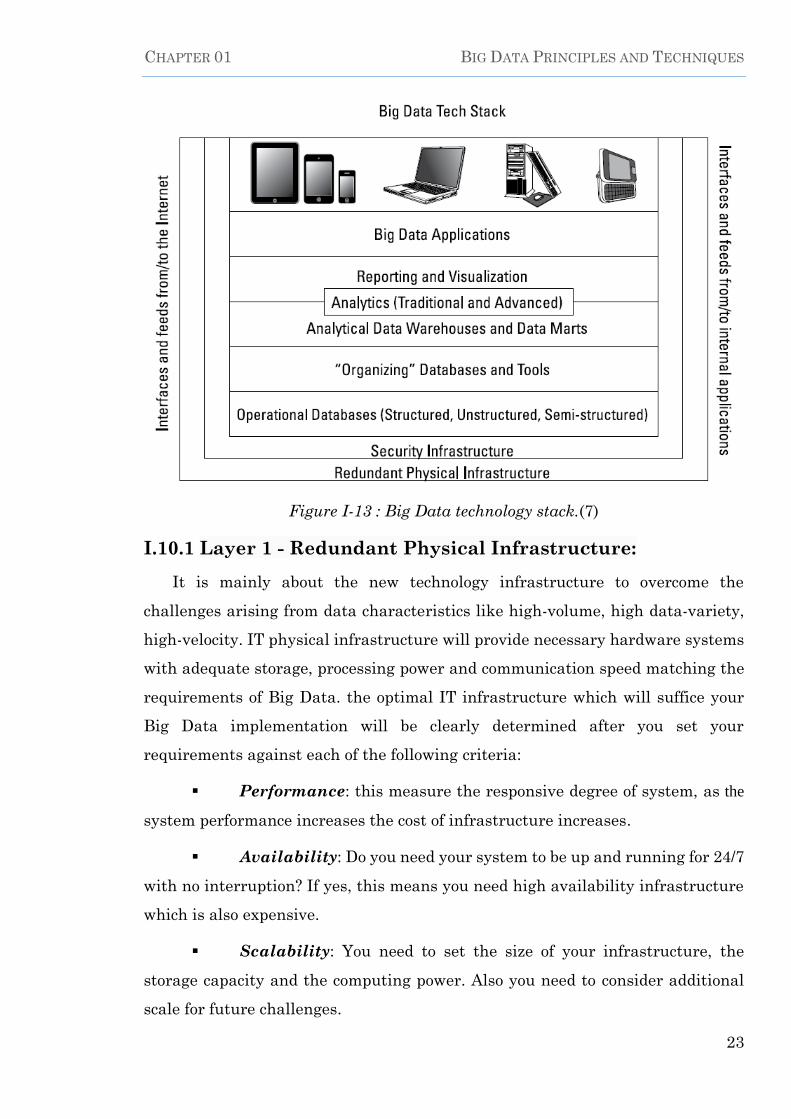
I.10 Big Data Technology Stack:
The task of getting useful insights out of Big Data is not easy. It is a matter of
developing comprehensive environment that includes hardware, infrastructure
software, operational software, management software and application
programming interface (API) to provide fully functional model managing the Big
Data requirements. the conceptual representation of this environment represented
as layered reference architecture is called big data technology stack, as shown in
Figure I-13, this technology stack is a comprehensive stack that has several
components that address specific functions of managing big data and tackle the
special need and challenges of it, these components are grouped in layers where
each layer performs a different function.(10) These layers work on the big data in
tandem to produce the desired results, these eight key layers of architecture are
as follows:
CHAPTER 01 BIG DATA PRINCIPLES AND TECHNIQUES
23
Figure I-13 : Big Data technology stack.(7)
I.10.1 Layer 1 - Redundant Physical Infrastructure:
It is mainly about the new technology infrastructure to overcome the
challenges arising from data characteristics like high-volume, high data-variety,
high-velocity. IT physical infrastructure will provide necessary hardware systems
with adequate storage, processing power and communication speed matching the
requirements of Big Data. the optimal IT infrastructure which will suffice your
Big Data implementation will be clearly determined after you set your
requirements against each of the following criteria:
Performance: this measure the responsive degree of system, as the
system performance increases the cost of infrastructure increases.
Availability: Do you need your system to be up and running for 24/7
with no interruption? If yes, this means you need high availability infrastructure
which is also expensive.
Scalability: You need to set the size of your infrastructure, the
storage capacity and the computing power. Also you need to consider additional
scale for future challenges.

CHAPTER 01 BIG DATA PRINCIPLES AND TECHNIQUES
24
Flexibility: this relates to how fast you can add more resources to
infrastructure or you can recover from failures. the flexibility degree is
pragmatically proportional with the cost, the most flexible infrastructures can be
costly, but we can control the costs with cloud services. Due to the non-stop flow of
data for Big Data projects the physical infrastructure must be both redundant and
resilient. Resiliency and redundancy are interrelated. An infrastructure, or a
system, is resilient to failure or changes when sufficient redundant resources are
in place, ready to jump into action.
I.10.2 Layer 2 – Security Infrastructure:
Security and privacy requirements for big data are similar to the requirements
for conventional data environments. The security requirements have to be closely
aligned to specific business needs. The following list describe briefly Some of the
unique challenges that arise when big data becomes part of the strategy:
1. Data access: User access to raw or computed big data has about the same
level of technical requirements as non-big data implementations. The data should
be available only to those who have a legitimate need for examining or interacting
with it.
2. Application access: Application access to data is also relatively
straightforward from a technical perspective. Most application programming
interfaces (APIs) offer protection from unauthorized usage or access.
3. Data encryption: The main solution to ensure the data remains protected
is to apply encryption however this is the most challenging aspect of security in a
big data environment, in traditional environments, encrypting and decrypting
data really stresses the system’s resources, With the volume, velocity, and
varieties associated with big data, this problem is exacerbated, the simplest
(brute-force) approach is to provide more and faster computational capability.
However, this comes with a steep price tag especially when you have to
accommodate resiliency requirements. A more temperate approach is to identify
the data elements requiring this level of security and to encrypt only the necessary
items.

CHAPTER 01 BIG DATA PRINCIPLES AND TECHNIQUES
25
4. Threat detection: The inclusion of mobile devices and social networks as
sources of big data exponentially increases both the amount of data and the
opportunities for security threats. It is therefore important that organizations take
a multi-perimeter approach to security.
I.10.3 Interfaces and Feeds to and from Applications and the
Internet (API’s):
So, the physical infrastructure enables everything and security infrastructure
protects all the elements in your big data environment. The next level in the stack
is the layer of interfaces and feeds to applications and the internet.
This layer manages the feed of data into and out of both internally managed
data and data feeds from external sources, since big data relies on the fact that
data from lots of sources are picked, this layer becomes critical for the big data
solutions, interfaces also exist at every level and between each layer of the stack,
without this layer big data cannot happen.
I.10.4 Layer 3 – Operational Databases:
At the heart of a big data environment are fast, scalable, and rock solid
database engines that contains the collections of data elements relevant to a
business. A choice has to be made between engines and database languages, a mix
of engines cloud also coexist within this layer.
For a long time, most of data management functionalities used to be provided
only by relational database management systems (RDBMS) and SQL, However,
in the last decades, new applications emerged and new requirements were raised
by big data that could hardly be met by relational databases thus the appearance
of NoSQL databases.
Let first consider Relational SQL Databases.
I.10.4.1 Relational Databases and RDBMS:
A relational database is a data store that organizes data using the relational
model, data is stored in database objects called tables. A table is a collection of
related data entries and it consists of columns and rows, and a schema strictly

CHAPTER 01 BIG DATA PRINCIPLES AND TECHNIQUES
26
defines the tables, columns, indexes, relationships between tables, and other
database elements.
SQL is the most widely used mechanism for creating, querying, maintaining,
and operating relational databases. These tasks are referred to as CRUD: Create,
retrieve, update, and delete, Optimization of queries, indexes and tables structure
is required to achieve peak performance, still this property however dependent of
the disk subsystem.
Relational databases management systems (RDBMS) support a set of
properties defined by the acronym ACID: Atomicity, Consistency, Isolation and
Durability.
Atomicity: A transaction is “all or nothing” when it is atomic. If any part of the
transaction or the underlying system fails, the entire transaction fails.
Consistency: Only transactions with valid data will be performed on the
database. If the data is corrupt or improper, the transaction will not complete and
the data will not be written to the database, data must conform to the schema.
Isolation: Multiple, simultaneous transactions will not interfere with each
other. All valid transactions will execute until completed and in the order they
were submitted for processing.
Durability: The ability to recover from an unexpected system failure or power
outage to the last known state.
A relational database is mostly suited when there is a need on gathering
business intelligence reports or in-depth analytics of large volumes of structured
data. Example of RDBMS include: SQL Server, MySQL, Oracle, PostgreSQL,
Even with all the features, relational databases are not capable to provide the
scale and agility needed to meet the challenges that face modern applications, nor
were they designed to take advantage of the inexpensive storage and processing
power that have become so readily available today.
Actually the features of such databases limit the feasibility and scalability of
it, as in order for example to maintain the ACID properties the database has to
pass through various parameters which limits its performance and also the

CHAPTER 01 BIG DATA PRINCIPLES AND TECHNIQUES
27
schema part is lacking, therefore the need for a new design that overcome those
limits, that brings us to talk about NoSQL databases.
I.10.4.2 NoSQL (Not Only SQL) databases:
NoSQL is the term used to describe high-performance, non-relational
databases which typically do not enforce a tabular schema of rows and columns
found in most traditional database systems, instead non-relational databases use
a storage model that is optimized for the specific requirements of the type of data
being stored.
Performance is generally a function of the underlying hardware cluster size,
network latency, and the calling application, NoSQL databases are designed to
scale out using distributed clusters of low-cost hardware to increase throughput
without increasing latency.
While RDBMS uses ACID (Atomicity, Consistency, Isolation, Durability) as a
mechanism for ensuring the consistency of data, non-relational DBMS use BASE,
which stands for Basically Available, Soft state, and Eventual Consistency. Of
these, eventual consistency is the most important, because it is responsible for
conflict resolution when data is in motion between nodes in a distributed
implementation. The data state is maintained by the software and the access
model relies on basic availability.
NoSQL is a better choice for businesses whose data workloads are more geared
toward the rapid processing and analyzing of vast amounts of varied and
unstructured data, e.g.: Big Data.
NoSQL databases do not use SQL for queries, and instead use other
programming languages and constructs to query the data, even though many of
these databases do support SQL-compatible queries. However, the underlying
query execution strategy is usually very different from the way a traditional
RDBMS would execute the same SQL query.
The following sections describe the major categories of NoSQL database:

CHAPTER 01 BIG DATA PRINCIPLES AND TECHNIQUES
28
Document Databases:
A document data store manages a set of named string fields and object data
values in an entity referred to as a document. These data stores typically store
data in the form of JSON documents. Each field value could be a scalar item, such
as a number, or a compound element, such as a list or a parent-child collection.
The data in the fields of a document can be encoded in a variety of ways, including
XML, YAML, JSON, BSON or even stored as plain text, document store does not
require that all documents have the same structure. This free-form approach
provides a great deal of flexibility. Documents are almost equivalent to records in
relational term, and collections are more similar to tables, whereas fields are
similar to attributes (columns) in each relation.(11)
Example of Document databases implementation include: MongoDB,
CouchDB.
Figure I-14 : A document can have many types of values : scalar , lists and nested
documents.
Columnar databases:
A columnar or column-family data store organizes data into columns and rows.
In its simplest form, a column-family data store can appear very similar to a
relational database, at least conceptually. The real power of a column-family
database lies in its denormalized approach to structuring sparse data, which stems
from the column-oriented approach to storing data, you can think of a column-
family data store as holding tabular data with rows and columns, but the columns

CHAPTER 01 BIG DATA PRINCIPLES AND TECHNIQUES
29
are divided into groups known as column families. Each column family holds a set
of columns that are logically related and are typically retrieved or manipulated as
a unit.
Figure I-15 : Columnar data store
The above diagram shows an example with two column
families, Identity and Contact Info . The data for a single entity has the same row
key in each column family. This structure, where the rows for any given object in
a column family can vary dynamically, is an important benefit of the column-
family approach, making this form of data store highly suited for storing data with
varying schemas.
The most popular columnar databases are HBase databases which relies
mainly on Hadoop file system and MapReduce for its operations. we will be
covering Hadoop and MapReduce in more details later in chapter 04, other
example of columnar databases include : Cassandra, AmazonSimpleDB.
Key/value databases:
A key/value store is essentially a large hash table. You associate each data
value with a unique key, and the key/value store uses this key to store the data by
using an appropriate hashing function. The hashing function is selected to provide
an even distribution of hashed keys across the data storage.
Key/value stores are highly optimized for applications performing simple
lookups using the value of the key, or by a range of keys, but are less suitable for
systems that need to query data across different tables of keys/values, such as

CHAPTER 01 BIG DATA PRINCIPLES AND TECHNIQUES
30
joining data across multiple tables.
One widely used open source key-value pair database is called Riak, other
examples include: Aerospike, LevelDB, DynamoDB.
Figure I-16 : Key/Value data store
Graph databases:
A graph data store manages two types of information, nodes and edges. Nodes
represent entities, and edges specify the relationships between these entities. Both
nodes and edges can have properties that provide information about that node or
edge, similar to columns in a table. Edges can also have a direction indicating the
nature of the relationship.
The purpose of a graph data store is to allow an application to efficiently
perform queries that traverse the network of nodes and edges, and to analyze the
relationships between entities. The following diagram shows an organization's
personnel data structured as a graph. The entities are employees and
departments, and the edges indicate reporting relationships and the department
in which employees work. In this graph, the arrows on the edges show the direction
of the relationships.(11)
Neo4J is the most widely used graph databases, other examples include :
ArangoDB, OrientDB, BrightstarDB, Meronymy.

CHAPTER 01 BIG DATA PRINCIPLES AND TECHNIQUES
31
Figure I-17 : Graph data store
Other examples of NoSQL database types include:
Multimodel Databases
Object Databases
Grid & Cloud Database
Solutions
XML Databases
Multidimensional Databases
Time Series / Streaming
Databases
Scientific and Specialized DBs
I.10.5 Layer 4 – Organizing Data Services and Tools:
Once you have understood what you need, what data you are gathering, where
to store it, and how to use it, you need to organize it so it can be consumed for
analytics, reporting, or specific applications, this is where this layer comes into the
picture.
Organizing data services and tools layer capture, validate, and assemble
various big data elements into contextually relevant collections, because big data
is massive, techniques have evolved to process the data efficiently and seamlessly.
Organizing data services are, in reality, an ecosystem of tools and technologies
that can be used to gather and assemble data in preparation for further processing.
As such, the tools need to provide integration, translation, normalization, and
scale. Technologies in this layer has to include the following:

CHAPTER 01 BIG DATA PRINCIPLES AND TECHNIQUES
32
A distributed file system: Necessary to accommodate the decomposition of
data streams and to provide scale and storage capacity
Serialization services: Necessary for persistent data storage and
Multilanguage remote procedure calls (RPCs)
Coordination services: Necessary for building distributed applications
(locking and so on).
Extract, transform, and load (ETL) tools: Necessary for the loading and
conversion of structured and unstructured data.
Workflow services: Necessary for scheduling jobs and providing a structure
for synchronizing process elements across layers.
In Chapters 4, we examine Hadoop, the most widely used set of products for
organizing big data.
I.10.6 Layer 5 – Analytical Data Warehouses and Data marts:
A data warehouse is a storage architecture designed to hold data extracted
from transaction systems, operational data stores, and external sources, the
warehouse then combines that data in an aggregate, summary form suitable for
enterprise-wide data analysis and reporting.
Before we present the component of a data warehouse, let review some
important concepts related to data warehousing for instance: OTLP and OLAP
and DataMarts.
IT systems could be divided into transactional systems (Online Transactions
Systems: OLTP) and analytical systems (Online Analytical Processing Systems:
OLAP). In general, we can assume that OLTP systems provide source data to data
warehouses, whereas OLAP systems help to analyze it.
OTLP: OLTP systems record business interactions as they occur in the day-
to-day operation of the organization, and support querying of this data to make
inferences, they are characterized by a large number of short on-line transactions
(INSERT, UPDATE, DELETE). The main emphasis for OLTP systems is put on
very fast query processing, maintaining data integrity in multi-access
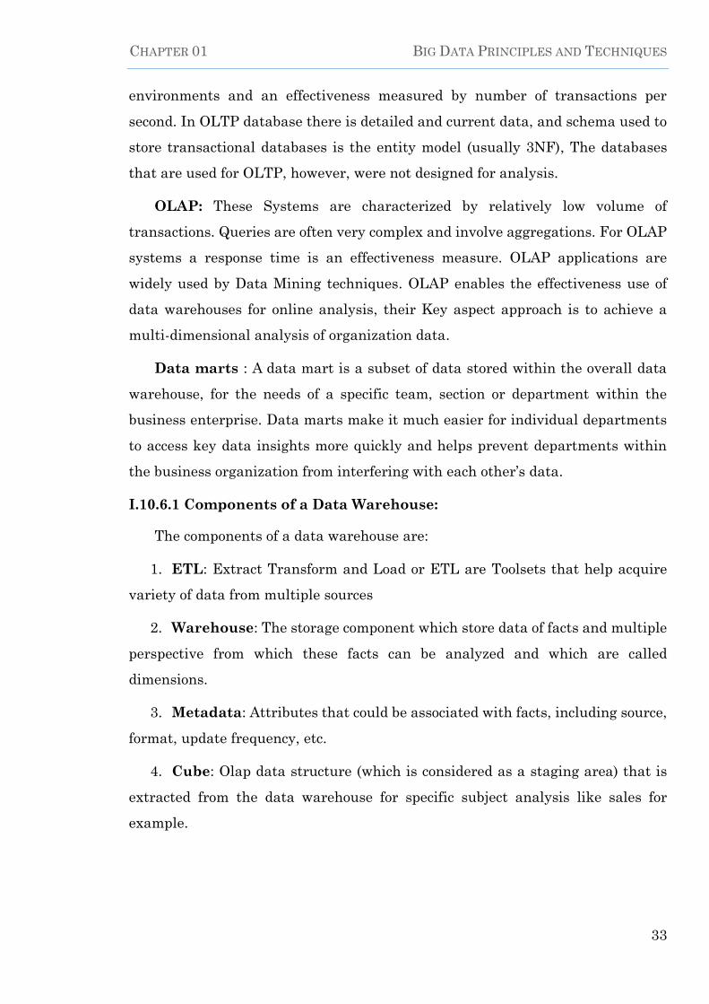
CHAPTER 01 BIG DATA PRINCIPLES AND TECHNIQUES
33
environments and an effectiveness measured by number of transactions per
second. In OLTP database there is detailed and current data, and schema used to
store transactional databases is the entity model (usually 3NF), The databases
that are used for OLTP, however, were not designed for analysis.
OLAP: These Systems are characterized by relatively low volume of
transactions. Queries are often very complex and involve aggregations. For OLAP
systems a response time is an effectiveness measure. OLAP applications are
widely used by Data Mining techniques. OLAP enables the effectiveness use of
data warehouses for online analysis, their Key aspect approach is to achieve a
multi-dimensional analysis of organization data.
Data marts : A data mart is a subset of data stored within the overall data
warehouse, for the needs of a specific team, section or department within the
business enterprise. Data marts make it much easier for individual departments
to access key data insights more quickly and helps prevent departments within
the business organization from interfering with each other’s data.
I.10.6.1 Components of a Data Warehouse:
The components of a data warehouse are:
1. ETL: Extract Transform and Load or ETL are Toolsets that help acquire
variety of data from multiple sources
2. Warehouse: The storage component which store data of facts and multiple
perspective from which these facts can be analyzed and which are called
dimensions.
3. Metadata: Attributes that could be associated with facts, including source,
format, update frequency, etc.
4. Cube: Olap data structure (which is considered as a staging area) that is
extracted from the data warehouse for specific subject analysis like sales for
example.
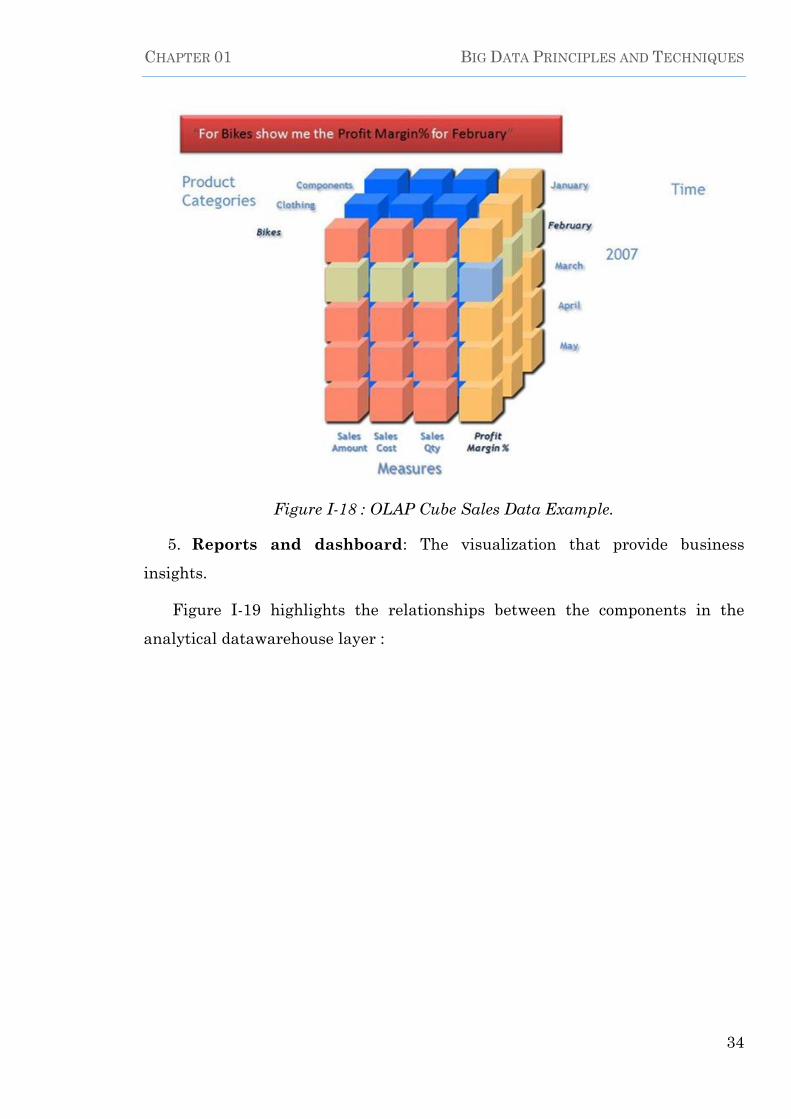
CHAPTER 01 BIG DATA PRINCIPLES AND TECHNIQUES
34
Figure I-18 : OLAP Cube Sales Data Example.
5. Reports and dashboard: The visualization that provide business
insights.
Figure I-19 highlights the relationships between the components in the
analytical datawarehouse layer :

CHAPTER 01 BIG DATA PRINCIPLES AND TECHNIQUES
35
Figure I-19 : Data Warehouse Component.
Data is complementary to become like a hybrid structure. This hybrid
structure will include highly structured data managed by traditional data
warehouse and the highly distributed and prone to change data is managed by
Hadoop-controlled solution.
I.10.7 Layer 6 – Analytics (Traditional and Advanced):
This layer contains analytics methods that reach into the data warehouses and
process the data for revealing insights, it contains business intelligence traditional
techniques as well as advanced data analytics methods.
I.10.7.1 BI vs. Analytics:
The increasing complexity of businesses problems, the possibility of several
alternatives solutions and the limited time available for making the right call in a
business scenario demands a highly structured decision-making process, most
businesses use huge amount of historical facts, figures, and data available for
informed decision making. This is called fact-based decision making and
collectively the set of tools, technique, and framework that allowed this is called
business intelligence or BI.
Organizations rely heavily on BI to run efficiently, and reducing decision cycle
time, however just making the right decision to run operations smartly is not

CHAPTER 01 BIG DATA PRINCIPLES AND TECHNIQUES
36
enough today, as a fiercely competitive world require businesses to use data
available beyond organizational data, and to foresee future trends, this is where
advanced analytics come into the picture.
I.10.7.2 Data Analytics Techniques:
Businesses today analyzes the growing volumes of unstructured and semi-
structured data available from multiple new sources such as machines, sensors,
logs, and social media, so let’s discuss a bit more about analytics.
Data analytics essentially include a set of statistical, mathematical modeling
methods and machine learning techniques and tools to analyze various types of
data in huge amounts.
I.10.7.3 Types of Analytical Applications and Techniques:
Analytical applications traditional and advanced typically fall under these
four categories depending on the level of answers:
Discovery analytics or BI.
Exploratory analysis or data
mining.
Predictive analytics.
Prescriptive analyti
Figure I-20 : Categories of Data Analytics Techniques.

CHAPTER 01 BIG DATA PRINCIPLES AND TECHNIQUES
37
Let’s cover each of these briefly:
1. Discovery analytics:
DA is the study of huge organizational data sets, some techniques that fall into
this category includes: slicing and dicing, roll ups and downs and business
graphics.
2. Exploratory analytics:
Goes a step further to analyze data deeper with techniques such as:
a. Statistical analytics: which involves collecting samples of data from a
bigger stat and scrutinizing it. this aims at identifying trends such as the primary
buyers of a certain brand of products over the last five years for example.
b. Text Analytics: this is the process of analyzing unstructured text,
extracting relevant information and transforming it into structured information,
that can then be leveraged in various ways, this can be used to detect plagiarism
in research papers.
c. Audio / Video Analytics: analyses audio and video data such as those from
traffic surveillance cameras, for security or vehicle classification purposes or to
analyses traffic density.
d. Unstructured data analytics: this helps extract structured information
from unstructured data, an example of this is fraud detection by analyzing credit
card data.
e. Email analytics: analyses the email data of customers or organization
which can help enhance marketing efforts, for instance use can use email analytics
applications to track the customers who read your emails and the ones who delete
it.
f. Association analytics: help finds interesting relationships in large data
sets for instance, analyses the purchases of consumers on a grocery store and
identify the goods they tend to buy together, this can help alter the layout of the
store to stock related items in one location.
g. Classification analytics: helps classify data, for instance, a marketing

CHAPTER 01 BIG DATA PRINCIPLES AND TECHNIQUES
38
manager can analyses customer profiles and classify the customers into categories
of the ones who will make a purchase and the ones who will not
h. Graph mining: graph mining along with subgraph mining are the subject
of this report and so will be covering them in much more details in the next
chapter.
3. Predictive analytics:
This is an advanced technique that aims to predict the probability of
occurrence of a future event such as loan defaults, stock market fluctuations and
so on, and thus taking preventive actions accordingly, some techniques that fall
into this category include:
Clustering and segmentation, creating decisions trees, predictive modeling.
4. Prescriptive analytics:
This helps analyze future trends to create strategies and find an optimal
solution to a problem or select an appropriate decision form multiple alternatives,
unlike predictive analytics that shows the probability of a future event
prescriptive analytics helps identify a solution to an existing problem for example
inventory management.
I.10.8 Layer 7 – Reporting and Visualization:
Reporting and dashboards: these are user-friendly tools used to
represent information collected from various sources. this area is still evolving to
support Big Data needs and currently it accesses new database technology
Visualization: these can be seen as advanced reporting tools which provide
pictorial or graphical representation for data and help users to easily understand
the data and relationship of several variables at the same time. the output of these
tools is greatly interactive and dynamic. these tools have employed new techniques
to enable users to watch the data as being changing in real time.
Visualization techniques include: mind maps, heap maps, infographic and
connection diagrams.

CHAPTER 01 BIG DATA PRINCIPLES AND TECHNIQUES
39
I.10.9 Layer 8 – Big Data Applications:
Users are most interested with the technology products relevant to this layer
as they are the end products which they interact with. these products can be third-
party applications or in-house applications which can fulfill common requirements
of multiple industries or the requirement of particular industry. Some examples
of well-known groups are log data application (Splunk, Loggly), marketing
applications (Bloomreach, Myrrix) and advanced Media applications (Bluefin,
DataXu). Building custom products for Big Data should follow up proper software
development standards, for example to include well-defined API interface which
will help the developers to access the functionalities exposed by each layer through
those interfaces
I.11 Virtualization and Cloud Computing in Big Data:
With the advent of big data, the nature and volume of data that the
organization received and needed to handle increased by multiple times this
required for constant upgradation of hardware and software to handle and analyze
the data effectively and efficiently.(12)
Traditionally businesses were incurring huge capital investments year-on-
year for purchasing and maintaining IT infrastructure and software to meet their
business needs, however this approach was not sustainable in the long run
businesses can no longer afford to start over and build all new applications every
time, a solution for this problem was found in the evolution of virtualization and
cloud computing technologies, these technologies enabled the system to support:
On-demand provisioning of resources
Full utilization of IT resources
Pay per use model of provisioning
IT infrastructure support as a service
Cloud computing and virtualization complement big data by enabling a global on-
demand network access to a shared pool of configurable computing resources.

CHAPTER 01 BIG DATA PRINCIPLES AND TECHNIQUES
40
I.11.1 Virtualization:
The term virtualization refers to the use of software to divide a pool of physical
infrastructure resources into several logical IT infrastructure resources.
With virtualization users can create many virtual systems within a single
physical system rather than assigning a dedicated set of physical resources to a
set of tasks, a pooled set of virtual resources are allocated as needed across all
workloads, virtualization also provide a level of automation and standardization
to optimize a computing environment, it supports the scalability and operating
efficiency required for big data and this is achieved by its three key
characterizations which are for instance partitioning, isolation and encapsulation.
1. Portioning: allows multiple applications and operating systems to exist in
a single physical system and share available resources.
2. Isolation: ensures that each virtual machine runs as a separate instance
and is isolated from the physical system and other virtual machines, thereby
minimizing the chances of crash or breach of data.
3. Encapsulation: enables the virtual machine to be presented to an
application as a complete entity, thereby protecting it from interference by other
applications.
Figure I-21 : Partitioning – Isolation – Encapsulation.

CHAPTER 01 BIG DATA PRINCIPLES AND TECHNIQUES
41
Some of the important benefits of virtualization includes:
Cost Saving.
Security.
Efficiency.
Enhanced speed.
Flexibility.
In order for the big data environments to scale almost without bounds, the
elements of it should be virtualized, this includes:
I.11.1.1 Server virtualization:
This involves the use of a software application that divides one physical server
into multiple isolated virtual environments. this ensures the scaling of the big data
environment to perform analysis of very large data sets.
I.11.1.2 Application virtualization:
Big data analysis may require independent deployment of different
applications, application virtualization encapsulates individual applications for
big data and removes their dependencies from the underlying physical computer
system. This in turn improves the overall manageability and portability of these
applications on different computers.
Figure I-22 : Application Virtualization.
Other than consolidation of servers and application virtualization, elements
than can be virtualized and which also have a positive impact on big data include
network, processors, memory, data, storage and desktop.
The table below lists this these elements along with their benefits:

CHAPTER 01 BIG DATA PRINCIPLES AND TECHNIQUES
42
Table I-2 : Virtualization of different elements.
.
I.11.2 Cloud Computing:
The generally accepted definition of cloud computing comes from the National
Institute of Standards and Technology NIST, it defines cloud computing as fellow:
“Cloud computing is a model for enabling convenient, on-demand network
access to a shared pool of configurable computing resources (e.g., networks,
servers, storage, applications and services) that can be rapidly provisioned and
released with minimal management effort or service provider interaction.”
What this means in plain terms is the ability to utilize parts of bulk resources
and that it enables rapid scaling of resources quickly and easily, often the term
cloud computing is wrongly used synonymously for virtualization and data center
however both are different technologies, let’s now look at the difference between a
data center and a cloud.(12)

CHAPTER 01 BIG DATA PRINCIPLES AND TECHNIQUES
43
I.11.2.1 Data Center vs. Cloud Computing:
A data center refers to on-premise or off-premise networked computer servers
used within an entreprise for the storage, processing and distribution of vast
amounts of data.
A cloud on the other hand is an off-premise internet computing that is used by
other external enterprises for storage, processing and distribution of vast amounts
of data.
Figure I-23 highlights some of their differences:
Figure I-23 : Data Center vs. Cloud Computing.
I.11.2.2 Cloud as a solution to big data requirements:
The benefits of cloud computing can be easily understood and appreciated
based on the requirements of big data analysis, for any big data implementation
availability of various components and a plan for their seamless integration and
ongoing maintenance is a must, cloud allows for self-provision cloud services this
automates and centralizes maintenance, software updates, configuration and
other management tasks, cloud computing provides high power servers for
analyzing big data in minutes, this rapid provisioning, scalability and elasticity is
a cost effective way to support big data technologies clear benefit of clouds for
handling big data analysis.

CHAPTER 01 BIG DATA PRINCIPLES AND TECHNIQUES
44
Finally, for reliability requirement of big data the cloud needs to provide fault
tolerance, by the mean of virtualization that help shared applications and
resources to coexist as independent virtual machines.
I.11.2.3 Cloud Computing Stack:
The broad collection of services that are made available to end users on a pay-
as-you-use model by the cloud is commonly referred to as cloud computing stack.
The stack shows three different categories within cloud computing, Software
as a service (SaaS), Platform as a service (PaaS), Infrastructure as a service
(IaaS).
Figure I-24 : Cloud Computing Stack.
1. Infrastructure as a Service (IaaS):
IaaS provides hardware, storage and network as a service examples include
virtual machines, load balancers and network attached storage a business for
example can save a lot on physical infrastructure by using a public cloud IaaS.
2. Platform as a Service (PaaS):
PaaS on the other hand provides a platform to write and run user’s
applications examples include Windows Azure and Google App Engine (GAE), note

CHAPTER 01 BIG DATA PRINCIPLES AND TECHNIQUES
45
that a platform here refers to the OS which is a collection of middleware services
and software development and deployment tools if an organization uses a private
cloud PaaS its programmers can create and deploy applications for its needs.
3. Software as a Service (SaaS):
Lastly SaaS provides software that can be accessed from anywhere for SaaS to
work however the infrastructure IaaS and the platform PaaS must be in place.
Organizations can choose where, when and how they use these services
however most organizations use all three services as infrastructure by itself isn’t
useful and idle till the platform and the necessary information or application is
made available for solving a particular problem.
I.11.2.4 Cloud Deployment models:
different deployment models exist in cloud computing which answer questions
of ownership, operations and usage.
1. Public Cloud:
One model is a public cloud which is owned and operated by an organization
for use by other organizations and individuals, a public cloud can customize
hardware and software to optimize performance however problems of security and
latency are an inherent part of public clouds.
2. Private Cloud:
A second cloud deployment model is a private cloud which is owned and
operated by an organization for its own purposes all stakeholders of an
organization have access to this cloud, a private cloud incorporates the systems
and processes of that organization and is highly automated and protected by
firewall, as a result latency is reduced and security is improved.
3. Hybrid Cloud:
Some organizations combine the two last mentioned models in what is called
a hybrid cloud, a number of connections are formed between the two clouds and
operations are automated to improve efficiency.

CHAPTER 01 BIG DATA PRINCIPLES AND TECHNIQUES
46
Key Points – Chapter 01 :
We presented the field of big data, gave a brief history of it and the
different definitions attributed by the practitioners in the field.
We defined the characteristics of big data for instance: Volume, Velocity
and Veracity.
We discussed big data types, structured / unstructured, at rest / in motion.
We presented the big data technology stack, which is comprehensive
environment that includes hardware infrastructure and software that
provide a fully functional model for managing the Big Data requirements.
We highlighted some databases technologies associated with big data as
well as some of the analytical methods traditional and advanced that help
derive insight and value from big data.
We Concluded the chapter by mentioning some of the benefits brought by
cloud computing and virtualization relative to big data.

47
Chapter II :
Graph Theory and Frequent
Subgraph Mining

CHAPTER 02 GRAPH THEORY AND FREQUENT SUBGRAPH MINING
48
II. Chapter 02 :
Graph Theory and Frequent Subgraph Mining
Context:
This Chapter defines in details the concept of graph mining and focus
primarily on frequent subgraph mining (FSM), it is organized in two parts:
Part 01 mainly dedicated to present, in a simplified way, the basic notions
related to graphs and graph theory.
Part 02, focus on presenting “the state of the art” of Frequent Subgraph mining
(FSM) algorithms and techniques. A survey of current research in the field, and
solutions to address the main research issues are also presented.
II.1 Data mining:
Data mining is a particular step in the process of Knowledge Discovery in
databases (KDD), which has a to extract statistically significant and useful
knowledge from a huge volume of raw data sets, extracting such important
knowledge can be crucial, sometimes essential, for the next phase in the analysis:
the modeling.(13) The KDD process is outlined in figure II-1.

CHAPTER 02 GRAPH THEORY AND FREQUENT SUBGRAPH MINING
49
Figure II-1: The steps of the KDD process.(14)
The additional steps in the KDD process include the data selection and
projection, and the visualization, and evaluation steps.
During the past decade, the field of data mining has emerged as a novel field
of research, investigating interesting research issues and developing challenging
real-life applications. The objective data formats in the beginning of data mining,
were limited to relational tables and transactions where each instance is
represented by one row in a table or one transaction represented as a set.
However, the studies within the last several years began to extend the classes
of considered data to semi-structured data such as HTML and XML texts, symbolic
sequences, and relations represented by advanced logics.
Frequent pattern mining for instance has been a focused theme in data mining
research for over a decade. Abundant literature has been dedicated to this
research and tremendous progress has been made, ranging from efficient and
scalable algorithms for frequent item set mining in transaction databases, mining
association rules, to numerous research frontiers, such as sequential pattern
mining. However, the arising and variety of the above-mentioned complex semi
structured data and the need of discovering structural patterns in large datasets,
which go beyond sets, sequences, and trees, toward complicated structure, makes
the frequent item sets and frequent sequence mining approaches inefficient and

CHAPTER 02 GRAPH THEORY AND FREQUENT SUBGRAPH MINING
50
unsuitable for such requirements, thus the emergence of graphs and frequent
structural mining as a solution to these concerns.
Certainly graphs as a data structure can meet the demands of modeling
complicated substructure patterns and relations among data, and they are
suitable representation for complex objects so from this perspective, there has
been much interest in the mining of graph data, (often referred to as graph based
data mining or shortly graph mining).
II.2 Graph mining:
Generally speaking, Graph mining is the process of discovering, retrieving and
analyzing non trivial patterns in graph shaped data. Graph based data mining or
graph mining has a strong relation with Multi-relational data mining. However,
the main objective of graph mining is to provide new principles and efficient
algorithms to mine topological substructures embedded in graph data, while the
main objective of multi-relational data mining is to provide principles to mine
and/or learn the relational patterns, represented by the expressive logical
languages, the former is more geometry oriented and the latter more logic and
relation oriented.(15)
Graph
Mining
Figure II-2 : Graph mining Related Concept

CHAPTER 02 GRAPH THEORY AND FREQUENT SUBGRAPH MINING
51
A number of popular research sub-domains of graph mining are listed in Table
Table II-1 : Graph mining research subdomains
Frequent subgraph mining(16–18)
Correlated graph pattern mining(19)
Optimal graph pattern mining(20)
Approximate graph pattern mining(21)
Graph pattern summarization(22)
Graph classification(23)
Graph clustering(24,25)
Graph indexing(26)
Graph searching(27,28)
Graph kernels(29–31)
Link mining(32–34)
Web structure mining(35)(36)
Work-flow mining(37)
Biological network mining(38)
II.3 Graphs applications:
Due to its capability of modeling complicated structures, graph representation
of data is well adopted and prevalent in a variety of domains including
wired/wireless interconnections (networks), 2D/3D objects (vision and pattern
recognition), chemical compounds/biological networks (chem/bio-informatics),
circuits (computer-aided design), loosely schemed data (XML), RDF data
(semantic web), program traces (software engineering), social media, etc.(39)
In chemistry for example chemical data, Chemical data (molecules,
compounds) is often represented as graphs in which the nodes correspond to
atoms, and the links correspond to bonds between the atoms.
Figure II-3 present a graph representation of a chemical compound:

CHAPTER 02 GRAPH THEORY AND FREQUENT SUBGRAPH MINING
52
Figure II-3 : Graph representation of a chemical compound.(13)
Benefiting from systems for searching and mining frequent pattern in
chemical compounds, researchers can do screening, designing, and knowledge
discovery in large-scale compound and molecular data sets.
Figure II-4 : Frequent subgraph mined from a variety of chemical compounds
In software engineering a program can be modeled by control flow graph where
basic blocks are represented as nodes and edges between nodes indicate the
possible flow of the program. Analysis of control flow graphs can shed light on the

CHAPTER 02 GRAPH THEORY AND FREQUENT SUBGRAPH MINING
53
static and dynamic behaviors of programs and aid in detecting malware and
viruses.
Additionally, advanced frequent patterns mining techniques can help us
understand different advanced functions and relations. For example, in a protein-
protein interaction network (PPI), a frequent pattern could uncover unknown
functions of a protein. Similarly, in a social network, a frequent pattern could show
a friend clique.
Figure II-5 shows a protein–protein interaction network, represented as a graph
where vertexes denote different proteins and the edges denote the physical
interactions between them, additionally Figure II-6 shows an example of a social
network graph representation.
Figure II-5 : Protein – Protein interaction network.

CHAPTER 02 GRAPH THEORY AND FREQUENT SUBGRAPH MINING
54
Social media networks (graphs), along with other example of recommendation
and knowledge graphs has the feature of being complex, ubiquitous and valuable,
therefore applying advanced mining techniques for finding frequent patterns that
specify a given minimum frequency constraint, could help reveal the rules that
derives their evolution.
1.5 Bln Users
450 Bln Relatioships
600 Mln Groups
313 Mln Users
500 Mln Tweets/day
Avg 208 followers/user
Figure II-6 : Social media graphs : there are complex Groups, links, preferences
and attributes.
Figure II-7 : Mining graph evolution rules.

CHAPTER 02 GRAPH THEORY AND FREQUENT SUBGRAPH MINING
55
II.4 What is Involved in graph mining:
Basic graph algorithms (shortest paths, BFS, DFS, isomorphisms,
traversals, random walks …)
Storage and indexing
Smart representations for compactness
Modeling of problems as graphs
Distance metrics and similarity measures
Exact, Approximate, and heuristic algorithms
Evolving structures
Interactivity and online updates
Complexity (most of the problems are not polynomially solvable)
II.5 Frequent subgraph mining (FSM):
Among the various kinds of graph pattern, frequent subgraphs are very basic
ones that can be discovered in a set of graphs (graph database) or a single large
graph, they are useful at characterizing graphs sets, discriminating different
groups of graphs, classifying and clustering graphs and building graphs indices,
frequent subgraph mining encompass all the techniques and methodologies used
to discover such patterns.(40)
Before diving into the details of the variant frequent subgraph mining
approaches and algorithms, let’s review first some of graph theory basic concepts
and terminologies.
II.6 Graph theory:
Graph theory is a branch of discrete mathematics that deals with the way
objects are connected. Thus, the connectivity in a system is a fundamental quality
of graph theory. The principal concept in graph theory is that of a graph. For a
mathematician, a graph is the application of a set on itself, i.e., a collection of
elements of the set and the binary relations between these elements. Graphs are

CHAPTER 02 GRAPH THEORY AND FREQUENT SUBGRAPH MINING
56
one-dimensional objects, but they can be embedded or realized in spaces of higher
dimensions.(41)
II.7 Preliminary definitions:
In the following paragraphs a number of widely used definitions, used later in
this chapter are introduced:
II.7.1 Types of graphs:
Generally speaking, a graph 𝑮 (𝑽, 𝑬) is defined to be a set 𝑉 of vertexes (nodes)
which are interconnected by a set 𝐸 of edges (links). The number of elements N in
V is called the order of 𝐺 and it is noted |𝑉| = 𝑁 and the number of elements 𝑀 in
𝐸 is the size of 𝐺 and it is noted |𝐸| = 𝑀.
Simple and multigraphs : In a graph 𝐺, when any two vertices of 𝑉 are
joined by more than one edge, the graph is called a multigraph. A graph without
loops and with at most one edge between any two vertices is called a simple
graph The graphs used in FSM are assumed to be labelled simple graphs.
In a graph 𝐺 (𝑉, 𝐸) for an edge 𝑒 = {𝑢, 𝑣}, we say:
- 𝑒 connects 𝑢 and 𝑣.
- 𝑢 and 𝑣 are end points of e.
- 𝑢 and e are incident (𝑣 and 𝑒 are incident).
- 𝑢 and 𝑣 are adjacent or neighbors.
(a) (b)
Figure II-8 : (a) Simple Graph, (b) nom simple graph having
multiple edge (left) nom simple graph having loops(right).

CHAPTER 02 GRAPH THEORY AND FREQUENT SUBGRAPH MINING
57
The degree deg(𝒗) of a vertex 𝑣 is the number of edges incident to it. A vertex
of degree 0 is called isolated.(42)
Regular Graphs : a graph 𝐺 in which all vertices are of equal degree is called
a regular graph, A regular graph of degree 𝑘 is also called 𝒌 − 𝑹𝒆𝒈𝒖𝒍𝒂𝒓.
Figure II-9 : 3-Regular graph k=3.
Labeled Graphs : A labelled graph can be represented as 𝐺(𝑉, 𝐸, 𝐿𝑉 , 𝐿𝐸 , 𝜑)
,where 𝑉 is a set of vertexes, 𝐸 𝑉 𝑥 𝑉 is a set of edges; 𝐿𝑉 and 𝐿𝐸 are sets of vertex
and edge labels. respectively; and 𝜑 is a label function that defines the mappings
𝑉 → 𝐿𝑉 and 𝐸 → 𝐿𝐸 , When the edge labels are members of an ordered set (e.g.,
the real numbers), a labeled graph may be called a weighted graph.(43)
Figure II-10 : Unlabeled and Labeled graphs.
Directed and undirected graphs : a graph 𝐺 is un- directed if ∀ 𝑒 𝜖 𝐸, 𝑒 is an un-
ordered pair of vertexes, and directed otherwise.

CHAPTER 02 GRAPH THEORY AND FREQUENT SUBGRAPH MINING
58
Walk, Trails , Paths and Cycles : A walk of a graph 𝐺 is an alternating
sequence of vertices and edges 𝑣0, 𝑒1, 𝑣1, …… . . , 𝑣𝑖−1, 𝑒𝑖, 𝑣𝑖 beginning and ending with
vertices, in which each edge is incident with two vertices immediately preceding
and following it. This walk joins the vertices 𝑣0 and 𝑣𝑖, and may also be denoted
by 𝑣1, 𝑣2, …… . . , 𝑣𝑖 (the edges being evident by context). The length 𝑙 of a walk is the
number of occurrences of edges in it; 𝑣0 is called the ini1ial vertex of the walk,
while 𝑣𝑖, is called the terminal vertex of the walk.
For example, the graph below outlines a possibly walk (in blue). The walk is
denoted as 𝑎𝑏𝑐𝑑𝑏. Note that walks can have repeated edges. For example, if we
had the walk 𝑎𝑏𝑐𝑑𝑐𝑏𝑐𝑒, then that would be perfectly fine even though some edges
are repeated.
In the graph above, the length of the walk is 𝑎𝑏𝑐𝑑𝑏 is 4 because it passes
through 4 edges.
A closed walk is a 𝑣𝑖 − 𝑣𝑖 walk, i.e., a walk which starts and ends at the same
vertex 𝑣𝑖, Otherwise, a walk is said to be open.
For example, the follow graph shows a closed walk in green:
Figure II-11 : Undirected graph (left), Directed graph (right).

CHAPTER 02 GRAPH THEORY AND FREQUENT SUBGRAPH MINING
59
Notice that the walk can be defined by 𝑐𝑒𝑔𝑓𝑐, and the start and end vertices of
the walk is c. Hence this walk is closed.
A walk is a trail if all the edges are distinct. So far, both of the earlier
examples can be considered trails because there are no repeated edges. Here is
another example of a trail:
Notice that the walk can be defined as 𝑎𝑏𝑐. There are no repeated edges so this
walk is also a trail.
Now let's look at the next graph:
Notice that this walk must repeat at least one edge.
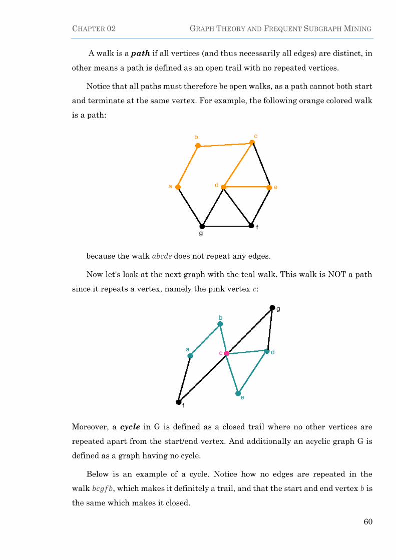
CHAPTER 02 GRAPH THEORY AND FREQUENT SUBGRAPH MINING
60
A walk is a path if all vertices (and thus necessarily all edges) are distinct, in
other means a path is defined as an open trail with no repeated vertices.
Notice that all paths must therefore be open walks, as a path cannot both start
and terminate at the same vertex. For example, the following orange colored walk
is a path:
because the walk 𝑎𝑏𝑐𝑑𝑒 does not repeat any edges.
Now let's look at the next graph with the teal walk. This walk is NOT a path
since it repeats a vertex, namely the pink vertex 𝑐:
Moreover, a cycle in G is defined as a closed trail where no other vertices are
repeated apart from the start/end vertex. And additionally an acyclic graph G is
defined as a graph having no cycle.
Below is an example of a cycle. Notice how no edges are repeated in the
walk 𝑏𝑐𝑔𝑓𝑏, which makes it definitely a trail, and that the start and end vertex b is
the same which makes it closed.
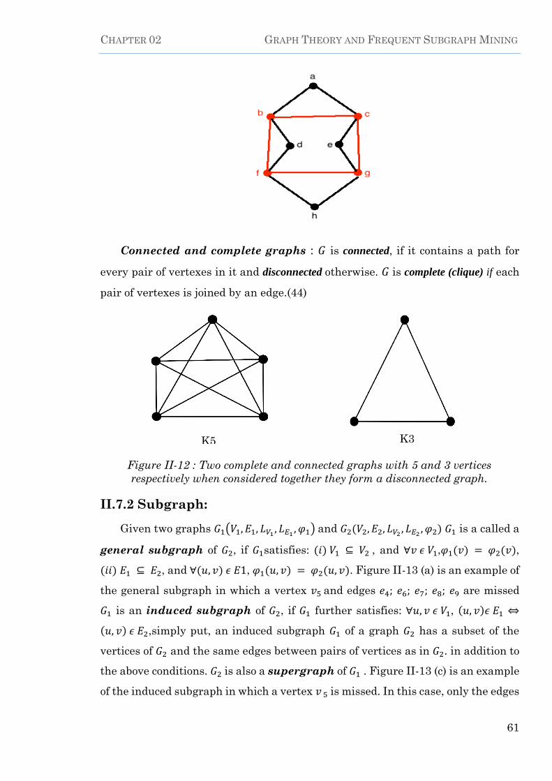
CHAPTER 02 GRAPH THEORY AND FREQUENT SUBGRAPH MINING
61
Connected and complete graphs : 𝐺 is connected, if it contains a path for
every pair of vertexes in it and disconnected otherwise. 𝐺 is complete (clique) if each
pair of vertexes is joined by an edge.(44)
II.7.2 Subgraph:
Given two graphs 𝐺1(𝑉1, 𝐸1, 𝐿𝑉1 , 𝐿𝐸1 , 𝜑1) and 𝐺2(𝑉2, 𝐸2, 𝐿𝑉2 , 𝐿𝐸2 , 𝜑2) 𝐺1 is a called a
general subgraph of 𝐺2, if 𝐺1satisfies: (𝑖) 𝑉1 ⊆ 𝑉2 , and ∀𝑣 𝜖 𝑉1,𝜑1(𝑣) = 𝜑2(𝑣),
(𝑖𝑖) 𝐸1 ⊆ 𝐸2, and ∀(𝑢, 𝑣) 𝜖 𝐸1, 𝜑1(𝑢, 𝑣) = 𝜑2(𝑢, 𝑣). Figure II-13 (a) is an example of
the general subgraph in which a vertex 𝑣5 and edges 𝑒4; 𝑒6; 𝑒7; 𝑒8; 𝑒9 are missed
𝐺1 is an induced subgraph of 𝐺2, if 𝐺1 further satisfies: ∀𝑢, 𝑣 𝜖 𝑉1, (𝑢, 𝑣)𝜖 𝐸1 ⇔
(𝑢, 𝑣) 𝜖 𝐸2,simply put, an induced subgraph 𝐺1 of a graph 𝐺2 has a subset of the
vertices of 𝐺2 and the same edges between pairs of vertices as in 𝐺2. in addition to
the above conditions. 𝐺2 is also a supergraph of 𝐺1 . Figure II-13 (c) is an example
of the induced subgraph in which a vertex 𝑣 5 is missed. In this case, only the edges
K5 K3
Figure II-12 : Two complete and connected graphs with 5 and 3 vertices
respectively when considered together they form a disconnected graph.

CHAPTER 02 GRAPH THEORY AND FREQUENT SUBGRAPH MINING
62
𝑒8 and 𝑒9 are also missed, and 𝑒4; 𝑒6; 𝑒7 are retained since they exist among 𝑣1; 𝑣3
and 𝑣4 in the original 𝐺.(43)
The third important and generic class of the substructure is a connected
subgraph where 𝑉1 ⊆ 𝑉2 , 𝐸1 ⊆ 𝐸 , and all vertices in 𝑉1 are mutually reachable
through some edges in 𝐸1. Figure II-13 (d) Is an example where 𝑣6 is further missed
from (c).
Figure II-13 : (a) a graph G , (b), (c) , (d) represent a general, induced, and
connected subgraphs respectively.(15)
II.7.3 Graph isomorphism:
A graph 𝐺1(𝑉1, 𝐸1, 𝐿𝑉1 , 𝐿𝐸1 , 𝜑1) is isomorphic to another graph
𝐺2(𝑉2, 𝐸2, 𝐿𝑉2 , 𝐿𝐸2 , 𝜑2) and is noted : 𝐺1 −̃ 𝐺2 if and only if a bijection f : 𝑉1 → 𝑉2 exists
such that: (𝑖) ∀ 𝑢 𝜖 𝑉1, 𝜙1(𝑢) = 𝜙2(𝑓(𝑢)), (𝑖𝑖)∀(𝑢, 𝑣) ∈ 𝐸1 ⇔ (𝑓(𝑢), 𝑓(𝑣)) 𝜖 𝐸2,
(𝑖𝑖𝑖) ∀(𝑢, 𝑣) ∈ 𝐸1, 𝜙1(𝑢, 𝑣) = 𝜙2(𝑓(𝑢), 𝑓(𝑣)). The bijection 𝑓 is an isomorphism
between 𝐺1and 𝐺2. A graph 𝐺1 is subgraph isomorphic to a graph 𝐺2, if and only
if there exists a subgraph 𝑔 ⊆ 𝐺2 such that 𝐺1 is isomorphic to g. In this case 𝑔 is
called an embedding of 𝐺1 in 𝐺2.(43)
Figure II-15, and Figure II-16 present respectively graph and subgraph
isomorphism:

CHAPTER 02 GRAPH THEORY AND FREQUENT SUBGRAPH MINING
63
Figure II-14 : Graph isomorphism.
The two graphs shown above are isomorphic, despite their different
looking drawings.
Figure II-15 : Subgraph Isomorphism.
Think of a graph isomorphism as of being a structure preserving bijection, and
it follows from the definition that the isomorphic graphs are identical, but
differently drawn, graphs.
Generally, the problem of recognizing isomorphic graphs is one of the grand
unsolved problems of graph theory. Construction of all N! possible mappings from
one graph to another (where N is the number of vertices), although obviously
impractical, remains as the only secure check for isomorphism of graphs.
𝜑
𝑔 𝐺1
𝐺2

CHAPTER 02 GRAPH THEORY AND FREQUENT SUBGRAPH MINING
64
An invariant of a graph 𝐺 is a quantity associated with 𝐺 which has the same
value for any graph isomorphic to 𝐺. Consequently, graph invariants are
quantities independent of the labeling of the vertices of a graph. Hence, the
number of vertices and the number of edges are invariants. A complete set of
invariants determines a graph up to isomorphism.
II.7.4 Automorphism:
An isomorphic mapping of the vertices of a graph 𝐺 onto themselves (which
also preserves the adjacency relationship) is called an automorphism of a graph
𝐺. Evidently, each graph possesses a trivial automorphism which is called the
identity automorphism. For some graphs, it is the only automorphism; these are
called identity graphs. The set of all automorphisms of a graph 𝐺 forms a group
which is called the automorphism group of 𝐺.(45)
II.7.5 Lattice:
Given a database 𝐺, a lattice is a structural form used to model the search
space for finding frequent subgraphs, where each vertex represents a connected
subgraph of the graph in 𝐺. The lowest vertex depicts the empty subgraph and the
vertexes at the highest level depict the graphs in 𝐺. A vertex 𝑝 is a parent of the
vertex 𝑞 in the lattice, if 𝑞 is a subgraph of 𝑝, and 𝑞 is different from 𝑝 by exactly
one edge. The vertex 𝑞 is a child of 𝑝. All the subgraphs of each graph 𝐺𝑖 𝜖 𝐺 which
occur in the database are present in the lattice and every subgraph occurs only
once in it.(43)

CHAPTER 02 GRAPH THEORY AND FREQUENT SUBGRAPH MINING
65
Figure II-16 : Lattice(G).
Example: given a graph data set 𝐺 = {𝐺1, 𝐺2, 𝐺3, 𝐺4}, the corresponding
Lattice(𝐺), is given in Figure II-16. In the figure, the lowest vertex ∅ represents
the empty subgraph, and the vertexes at the highest level correspond to 𝐺1, 𝐺2, 𝐺3,
and 𝐺4. The parents of the subgraph 𝐵 − 𝐷 are subgraphs 𝐴 − 𝐵 − 𝐷 (joining the
edge 𝐴 − 𝐵) and 𝐵 − 𝐷 − 𝐺 (joining the edge 𝐷 − 𝐺). Similarly, subgraphs 𝐵 − 𝐶 and
𝐶 − 𝐹 are the children of the subgraph 𝐵 − 𝐶 − 𝐹.
II.7.6 Density:
The density of a graph 𝑮 = (𝑽; 𝑬) is calculated by:
𝑑𝑒𝑠𝑛𝑠𝑖𝑡𝑦(𝐺) = 2 .|𝐸|
(|𝑉| . (|𝑉| − 1)).
The graph density measures the ratio of the number of edges compared to the
maximal number of edges in a complete graph. A graph is said to be dense if the
ratio is close to 1, and is considered as sparse if the ratio is close to 0.(13)
II.7.7 Trees:
Free Tree: a free tree is defined as an undirected graph that is connected and
acyclic.
Labelled Unordered Tree: A labeled unordered tree (an unordered tree, for
short) is directed acyclic graph denoted as 𝑇(𝑉, 𝜑, 𝐸, 𝑣𝑟), where 𝑉 is a set of vertexes
of 𝑇; 𝜑 is a labeling function, such that ∀𝑣𝑖 ∈ 𝑉, 𝜑(𝑣𝑖) → 𝑣𝑖; 𝐸 ⊆ 𝑉 × 𝑉 is a set of
CHAPTER 02 GRAPH THEORY AND FREQUENT SUBGRAPH MINING
66
edges of 𝑇; and 𝑣𝑟 is a distinguished vertex called root of 𝑇. For ∀𝑣𝑖 ∈ 𝑉, there is a
unique path (𝑣𝑟 , 𝑣1, 𝑣2, …… . . , 𝑣𝑖) from the root 𝑣𝑟 to 𝑣𝑖. If a vertex 𝑣𝑖 is on the path
from the root to the vertex 𝑣𝑗 , then 𝑣𝑖 is an ancestor of 𝑣𝑗 , and 𝑣𝑗 is a descendant of
𝑣𝑖. For each edge (𝑣𝑖 , 𝑣𝑗) 𝜖 𝐸 , 𝑣𝑖 is the parent of 𝑣𝑗, and 𝑣𝑗 is a child of 𝑣𝑖. Vertexes
that share the same parent are siblings. The size of 𝑇 is defined to be the number
of vertexes in 𝑇. A vertex without any child is a leaf vertex; otherwise it is an
intermediate vertex. The right most path of 𝑇 is the path from the root vertex to the
rightmost leaf. The depth(level) of a vertex is the length of the path from the root to
that vertex.
Labelled Ordered Tree: A labelled ordered tree (an ordered tree, for short)
is a labelled unordered tree but with a left-to-right ordering imposed among the
children of each vertex.
Other form of subtrees includes: Bottom-up subtree, Induced Subtree and
embedded Subtree.
II.8 Overview of FSM:
Frequent Subgraph Mining (FSM) is the essence of graph mining, The field of
study concentrates on the identification of frequent subgraphs within graph data
sets. The research goals are directed at: (i) effective mechanisms for generating
candidate subgraphs (without generating duplicates) and (ii) how best to process
the generated candidate subgraphs so as to identify the desired frequent
subgraphs in a way that is computationally efficient and procedurally effective.
frequent subgraphs are considered so, if their counts are above a minimum
support threshold. Figure II-8 (a) presents an overview of the domain of FSM in
terms of the number of significant FSM algorithms that have been proposed over
the period 1994 to the present. From the figure we can see periods of activity in
the early 90s (coinciding with the introduction of the concept of data mining)
followed by another period of activity from 2002 to 2007. No “new” algorithms have
been introduced over the past few years, indicating that the field is reaching
maturity, although there has been much work focused on variations of existing
algorithms.

CHAPTER 02 GRAPH THEORY AND FREQUENT SUBGRAPH MINING
67
Other than the research activity associated with FSM the importance of FSM
is also reflected in its many areas of its application. Figure II-8 (b) presents an
overview of the application domain of FSM in terms of the number of FSM
algorithms reported in the literature and the specific application domain at which
they have been directed. From the figure it can be seen that three application
domains (chemistry, web, and biology) dominated the usage of FSM algorithms.
The straightforward idea behind FSM is to “grow” candidate subgraphs, in
either a breadth first (BFS) or depth first (DFS) manner (candidate generation),
and then determine if the identified candidate subgraphs occur frequently enough
in the graph data set for them to be considered interesting (support counting). The
two main research issues in FSM are thus how to efficiently and effectively:
(i) Generate the candidate frequent subgraphs.
(ii) Determine the frequency of occurrence of the generated subgraphs.(43)
Effective candidate subgraph generation requires that the generation of duplicate
or superfluous candidates is avoided. Occurrence counting requires repeated
comparison of candidate subgraphs with subgraphs in the input data, a process
known as isomorphism checking. FSM, in many respects, can be viewed as an
extension of Frequent Itemset Mining (FIM) popularized in the context of
association rule mining (see for example (46)). Consequently, many of the proposed
solutions to addressing the main research issues effecting FSM are based on
0
2
4
6
8
10
12
(a) Year
0
5
10
15
20
25
(b) Application
Figure II-17 : The distribution of the most significant FSM algorithms with
respect to year of introduction and application domain.

CHAPTER 02 GRAPH THEORY AND FREQUENT SUBGRAPH MINING
68
similar techniques found in the domain of FIM. For example, the downward
closure property (DCP) associated with itemsets has been widely adopted with
respect to candidate subgraph generation, we will define it later in the chapter.
II.9 Formalism:
There are two separate problem formulations for FSM: (i) graph transaction
based FSM and (ii) single graph based FSM. In graph transaction based FSM, the
input data comprises a collection of medium-size graphs called transactions. Note
that the term “transaction” is borrowed from the field of Association Rule
Mining.(47)
In single graph based FSM the input data, as the name implies, comprises one
very large graph.
A subgraph 𝑔 is considered to be frequent if its occurrence count is greater than
some predefined threshold value. The occurrence count for a subgraph is usually
referred to as its support, and the consequently the threshold is referred to as the
support threshold. The support of 𝑔 may be computed using either transaction-based
counting or occurrence-based counting. Transaction based counting is only applicable
to graph transaction based FSM, while occurrence-based counting may be applied
to either transaction based FSM or single graph based FSM. However, occurrence-
based counting is typically used with single graph based FSM.
In transaction-based counting the support is defined by the number of graph
transactions that 𝑔 occurs in, one count per transaction regardless of whether 𝑔
occurs once or more than once in a particular graph transaction. Thus, given a
database 𝐺 = {𝐺1, 𝐺2, 𝐺3… . . , 𝐺𝑇} consisting of a collection of graph transactions,
and a support threshold 𝜎 𝜖 [0,1] then the set of graph transactions where a
subgraph 𝑔 occurs is defined by 𝛿𝐺(𝑔) = {𝐺𝑖|𝑔 ⊆ 𝐺𝑖 }. Thus, the support of 𝑔 is
defined as:
𝑠𝑢𝑝𝐺(𝑔) = |𝛿𝐺(𝑔)|/𝑇
where |𝛿𝐺(𝑔)| denotes the cardinality of 𝛿𝐺(𝑔) and 𝑇 the number of graphs
(transactions) in 𝐺. Therefore, 𝑔 is frequent if and only if 𝑠𝑢𝑝𝐺(𝑔) ≥ 𝜎. In

CHAPTER 02 GRAPH THEORY AND FREQUENT SUBGRAPH MINING
69
occurrence-based counting we simply count up the number of occurrences of 𝑔 in
the input set, (note that we are interested only on the transaction based FSM in
this report.)
Transaction-based counting offers the advantage that the well-known
Downward closure property can be employed to significantly reduce the computation
overhead associated with candidate generation in FSM. In the case of occurrence-
based counting, either an alternative frequency measure, which maintains the DC
property, must be established; or some heuristics adopted to keep the computation
as inexpensive as possible.(43)
II.10 Graph isomorphism detection:
The kernel of FSM is (sub)graph isomorphism detection. Graph isomorphism is
neither known to be solvable in polynomial time nor NP-complete, while subgraph
isomorphism, where we wish to establish whether a subgraph is wholly contained
within a super graph, is known to be NP-complete (48). When restricting the
graphs to trees, (sub)graph isomorphism detection becomes (sub)tree isomorphism
detection. Tree isomorphism detection can be solved in a linear time.
Subgraph isomorphism detection is fundamental to FSM. A significant
number of “efficient” techniques have been proposed, all directed at reducing, as
far as possible, the computational overhead associated with it. Subgraph
isomorphism detection techniques can be roughly categorized as being either:
exact matching (49–53) or error tolerant matching (54–57). Most FSM algorithms
adopt exact matching. A categorization of the main exact matching subgraph
isomorphism detection algorithms is presented in Table 2.
Table II-2 : Categorization of exact matching (sub) graph isomorphism testing
algorithms.
Algorithms Main Techniques Matching Types
Ullman Backtracking + look ahead Graph & subgraph isomorphism
SD Distance matrix + backtracking Graph isomorphism
Nauty Group theory + canonical labeling Graph isomorphism

CHAPTER 02 GRAPH THEORY AND FREQUENT SUBGRAPH MINING
70
VF DFS strategy + feasibility rules Graph & subgraph isomorphism
VF2 VF’s rationate + advanced data
structures
Graph & subgraph isomorphism
With reference to Table 2, Ullmann’s algorithm employs a backtracking
procedure with a look-ahead function to reduce the size of the search space (49).
The SD algorithm, in turn, utilizes a distance matrix representation of a graph
with a backtracking procedure to reduce the search (50). The Nauty algorithm
(51) uses group theory to transform graphs to be matched into a canonical form so
as to provide for more efficient and effective graph isomorphism checking.
However, it has been noted (58) that the construction of the canonical forms can
lead to exponential complexity in the worst case. Although Nauty was regarded as
the fastest graph isomorphism algorithm by Conte (58), Miyazaki in (59)
demonstrated that there exist some categories of graphs which required
exponential time to generate the canonical labelling. The VF (52) and VF2 (53)
use a Depth First Search (DFS) strategy, assisted by a set of feasibility rules to
prune the search tree. VF2 is an improved version of VF, that explores the search
space more effectively so that the matching time and the memory consumption are
significantly reduced.
II.11 Search strategy:
There are two basic search strategies employed for mining frequent
subgraphs, the depth first search (DFS) strategy and the breadth first search
(BFS) strategy.
The Depth First Search (DFS) strategy is a method for traversing or searching
tree or graph data structures. It starts at the root (selecting a node as the root in
the graph case) and explores as far as possible along each branch before
backtracking.
the Breadth First Search (BFS) uses the opposite strategy that is performed
by DFS. It starts at the tree root (or some arbitrary node of a graph, sometimes
referred to as a ‘search key’), and explores all of the neighbor nodes at the present

CHAPTER 02 GRAPH THEORY AND FREQUENT SUBGRAPH MINING
71
depth prior to moving on to the nodes at the next depth level. Figure II-9 Illustrate
the process of DFS and BFS.
Figure II-18 : DFS and BFS search strategies.
II.12 FSM algorithmic approaches:
This section provides a generic overview of the process of FSM, it is widely
accepted that FSM techniques can be divided into two categories:
(i) Apriori-based approaches.
(ii) Pattern growth-based approaches.
These two categories are similar in spirit to counterparts found in Association
Rule Mining (ARM), namely the Apriori algorithm (46) and FP-growth algorithm
(60) respectively. Before defining each of them let’s review first the apriority
property.
II.12.1 Apriori Property:
The Apriori property also known as the downward closure property (DCP),
expresses a monotonic decrease of an evaluation criterion accompanying with the
progress of a sequential pattern mining. It is activated in order to efficiently
discover all frequent sequential patterns, in simple terms this property impose
that if a graph is frequent, then all of its subgraphs will also be frequent, thus the
frequency or the support of a sequential graph is always decreasing or remaining
constant, and never increases to overpass the support of its parent subgraphs.

CHAPTER 02 GRAPH THEORY AND FREQUENT SUBGRAPH MINING
72
This property must be hold for both the Apriori and the Pattern growth based
algorithms to safely prune the candidates that are not frequent.
II.12.2 Apriori based approach:
The Apriori-based approach proceeds in a generate-and-test manner using a
Breadth First Search (BFS) strategy to explore the subgraph lattice of the given
database. Therefore, before considering (𝑘 + 1) subgraphs, this approach has to
first consider all 𝑘 subgraphs.(43)
The general framework of Apriori-based algorithms is outlined in the
Algorithm AprioriGraph below:
Figure II-19 : Apriori Algorithm.

CHAPTER 02 GRAPH THEORY AND FREQUENT SUBGRAPH MINING
73
Let 𝑆𝑘 be the frequent subgraph set of size 𝑘, the Algorithm AprioriGraph
adopts a level-wise mining methodology. At each iteration, the size of newly
discovered frequent subgraphs is increased by one. These new subgraphs are first
generated by joining two similar frequent subgraphs that are discovered in the
last call of the Algorithm. The newly formed graphs are then checked for their
frequency. The frequent ones are used to generate larger candidates in the next
round. The main design complexity of Apriori-based algorithms comes from the
candidate generation step. Although the candidate generation for frequent itemset
mining is straightforward, the same problem in the context of graph mining is
much harder, since there are many ways to merge two graphs. The diagram of
figure II-10 highlight the Apriori subgraph generation method.
II.12.3 Pattern Growth Approach:
The pattern growth-based adopts a DFS or BFS strategies to explore the
subgraph lattice, and for each discovered subgraph 𝑔, the subgraph is extended
recursively until all frequent supergraphs of 𝑔 are discovered.
Algorithm PatternGrowthGraph illustrates a framework of pattern growth-
based frequent graph mining algorithms. A graph 𝑔 can be extended by adding a
new edge 𝑒. The newly formed graph is denoted by 𝑔 𝑥 𝑒 . Edge 𝑒 may or may not
introduce a new vertex to 𝑔. For each discovered graph 𝑔, PatternGrowth performs
extensions recursively until all the frequent graphs with 𝑔 embedded are
discovered. The recursion stops once no frequent graph can be generated any more.
Figure II-20 : Apriori-based Approach.

CHAPTER 02 GRAPH THEORY AND FREQUENT SUBGRAPH MINING
74
Figure II-21 : PatternGrowth algorithm.
The Algorithm above is simple, but not efficient. The bottleneck is at the
inefficiency of extending a graph. The same graph can be discovered many times.
For example, there may exist 𝑛 different (𝑛 − 1) −edge graphs which can be
extended to the same 𝑛 −edge graph. The repeated discovery of the same graph is
computationally inefficient. A graph that is discovered at the second time is called
duplicate graph. Although Line 1 of the Algorithm gets rid of duplicate graphs, the
generation and detection of duplicate graphs may cause additional workloads. In
order to reduce the generation of duplicate graphs, each frequent graph should be
extended as conservatively as possible in a sense that not every part of each graph
should be extended.
The diagram of figure II-11 highlight the pattern growth subgraph generation
method.

CHAPTER 02 GRAPH THEORY AND FREQUENT SUBGRAPH MINING
75
Figure II-22 : PatternGrowth-based approach.
II.13 Basic Framework of FSM algorithms:
Most existing FSM algorithms (both Apriori and Pattern growth) adopt an
iterative pattern mining strategy where each iteration can be divided into two
phases: (i) candidate generation, and (ii) support computation, Generally, research
on FSM focuses on these two phases using a variety of techniques. Since it is
harder to address subgraph isomorphism detection, more research effort is
directed at how to efficiently generate subgraph candidates. Because subtree
isomorphism detection can be solved in 𝑂 (𝑘1.5
log 𝑘 𝑛) time, the computational
complexity is reduced within the context of FSM.(43)
Figure II-23 highlight the basic framework adopted by the most FSM
algorithms:
𝑭𝒓𝒆𝒒𝒖𝒆𝒏𝒕_𝑺𝒖𝒃𝒈𝒓𝒂𝒑𝒉_𝑴𝒊𝒏𝒊𝒏𝒈 (𝑮,𝒎𝒊𝒏𝒔𝒖𝒑)
//𝑮 𝒊𝒔 𝒅𝒂𝒕𝒂𝒃𝒂𝒔𝒆 𝒄𝒐𝒏𝒕𝒂𝒊𝒏𝒊𝒏𝒈 𝒈𝒓𝒂𝒑𝒉𝒔 𝒅𝒂𝒕𝒂𝒔𝒆𝒕𝒔.
𝟎 – 𝑴𝒊𝒏𝒊𝒏𝒈 𝒔𝒕𝒂𝒓𝒕𝒔 𝒘𝒊𝒕𝒉 𝒇𝒓𝒆𝒒𝒖𝒆𝒏𝒕 𝒑𝒂𝒕𝒕𝒆𝒓𝒏 𝒐𝒇 𝒔𝒊𝒛𝒆 𝟏 𝒊. 𝒆. 𝑭𝟏 (𝑷𝒐𝒑𝒖𝒍𝒂𝒕𝒆 𝑭𝟏)
𝟏 – 𝒘𝒉𝒊𝒍𝒆 𝑭𝒌 ≠ ∅
𝟐 – 𝑪𝒌+𝟏𝑪𝒂𝒏𝒅𝒊𝒅𝒂𝒕𝒆_𝒈𝒆𝒏𝒆𝒓𝒂𝒕𝒊𝒐𝒏(𝑭𝒌 , 𝑮)
𝟐 – 𝒇𝒐𝒓𝒂𝒍𝒍 𝒄 𝒊𝒏 𝑪𝒌+𝟏
𝟑 – 𝒊𝒇 𝒊𝒔𝒐𝒎𝒐𝒓𝒑𝒉𝒊𝒔𝒎_𝒄𝒉𝒆𝒄𝒌𝒊𝒏𝒈(𝒄) = 𝒕𝒓𝒖𝒆
𝟒 – 𝒔𝒖𝒑𝒑𝒐𝒓𝒕_𝒄𝒐𝒖𝒏𝒕𝒊𝒏𝒈(𝒄, 𝑮)
𝟓 – 𝒊𝒇 𝒄. 𝒔𝒖𝒑 >= 𝒎𝒊𝒏𝒔𝒖𝒑

CHAPTER 02 GRAPH THEORY AND FREQUENT SUBGRAPH MINING
76
𝟔 – 𝑭𝒌+𝟏 = 𝑭𝒌+𝟏⋃𝒄
𝟕 – 𝒌 = 𝒌 + 𝟏
𝟖 – 𝒓𝒆𝒕𝒖𝒓𝒏 𝒔𝒆𝒕 𝒐𝒇 𝒇𝒓𝒆𝒒𝒖𝒆𝒏𝒕 𝒑𝒂𝒕𝒕𝒓𝒏𝒔 ⋃ 𝑭𝒊𝒊=𝟏,….𝒌−𝟏
Figure II-23 : Baseline algorithm for FSM.
Before presenting a survey of the most FSM algorithms in literature, essential
techniques used to support their operations are first presented, such techniques
allow achieving:
01 – Efficient candidate generation.
02 – Isomorphism checking.
03 – Support computation.
representation of graphs will first be considered. The aim here is to represent
graphs in such a manner that subgraphs can be enumerated efficiently so as to
facilitate the desired FSM and facilitate isomorphism checking on subgraphs.
II.13.1 Canonical Representations:
The simplest mechanism whereby a graph structure can be represented is by
employing an adjacency matrix or adjacency list.
an adjacency matrix is a square matrix used to represent a finite graph. The
elements of the matrix indicate whether pairs of vertices are adjacent or not in the
graph. In the special case of a finite simple graph, the adjacency matrix is a (0,1)-
matrix with zeros on its diagonal. If the graph is undirected, the adjacency matrix
is symmetric.
an adjacency list is a collection of unordered lists used to represent a
finite graph. Each list describes the set of neighbors of a vertex in the graph, There
are many variations of this basic idea, differing in the details of how they
implement the association between vertices and collections, in how they
implement the collections, in whether they include both vertices and edges or only
vertices as first class objects, and in what kinds of objects are used to represent

CHAPTER 02 GRAPH THEORY AND FREQUENT SUBGRAPH MINING
77
the vertices and edges. Figure II-12 present a simple graph G along with its
corresponding adjacency matrix.
(
𝑎 1 0 1 0 0 0 1 0 01 𝑏 0 0 1 0 0 0 0 00 0 𝑐 0 1 1 0 0 0 01 0 0 𝑑 0 1 1 0 0 00 1 1 0 𝑒 1 0 0 0 00 0 1 1 1 𝑓 1 1 0 10 0 0 1 0 1 𝑔 0 0 01 0 0 0 0 1 0 ℎ 1 00 0 0 0 0 0 0 1 𝑘 00 0 0 0 0 1 0 0 0 𝑤)
Throughout this section Graph G will be used to illustrate the canonical
representations discussed, for ease of illustration, all edge labels are assumed to
be the same and are represented by “1”.
The use of the adjacency matrices and adjacency lists, although
straightforward, it does not lend itself to isomorphism detection, because a graph
can be represented in many different ways depending on how the vertexes (and
edges) are enumerated. With respect to isomorphism testing it is therefore
desirable to adopt a consistent labelling strategy that ensures that any two
identical graphs are labelled in the same way regardless of the order in which
vertexes and edges are presented (i.e. a canonical labelling strategy).
A canonical labelling strategy defines a unique code for a given graph,
Canonical labelling facilitates isomorphism checking because it ensures that if a
pair of graphs are isomorphic, then their canonical labellings will be identical. One
simple way of generating a canonical labelling is to flatten the associated
adjacency matrix by concatenating rows or columns to produce a code comprising
a list of integers with a minimum (or maximum) lexicographical ordering imposed.
To further reduce the computation resulting from the permutations of the matrix,
canonical labellings are usually compressed, using what is known as a vertex
(a) Graph G with preorder subscript (b) G’s adjacency matrix
Figure II-24 : A simple graph G with its corresponding adjacency matrix.

CHAPTER 02 GRAPH THEORY AND FREQUENT SUBGRAPH MINING
78
invariant scheme (61), that allows the content of an adjacency matrix to be
partitioned according to the vertex labels. Various canonical labelling schemes
have been proposed, some of the more significant are described in this subsection.
Minimum DFS Code (M-DFS):
There are a number of variants of DFS encodings, but essentially each vertex
is given a unique identifier generated from a DFS traversal of a graph (DFS
subscripting). Each constituent edge of the graph in the DFS code is then
represented by a 5-tuple: (𝑖, 𝑗, 𝑙𝑖 , 𝑙𝑒 , 𝑙𝑗 ) where 𝑖 and 𝑗 are the vertex identifiers,𝑙𝑖
and 𝑙𝑗 are the labels for the corresponding vertexes, and 𝑙𝑒 is the label for the edge
connecting the vertexes. Based on the DFS lexicographic order, the M-DFSC of a
graph 𝑔 can be defined as the canonical labelling of 𝑔 (17). The DFS codes for the
left-most branch and the right-most branch of the example graph if figure II-24 (a)
are : {(0, 1, a, 1, b), (1, 2, b, 1, e), (2, 3, e, 1, f), (3, 4, f, 1, c), (4, 2, c, 1, e)} and
{(0, 9, a, 1, d), (9, 10, d, 1, f), (10, 11, f, 1, g), (11, 9, g, 1, d)} respectively.
The algorithm FSM-H under study utilize M-DFS code as its coding scheme to
issue isomorphism checking on candidate patterns.
Canonical Adjacency Matrix (CAM):
Given an adjacency matrix 𝑀 of a graph 𝑔, an encoding of 𝑀 can be obtained
by the sequence obtained from concatenating the lower (or upper) triangular
entries of 𝑀, including entries on the diagonal. Since different permutations of the
set of vertexes correspond to different adjacency matrices, the canonical (CAM)
form of 𝑔 is defined as the maximal (or minimal) encoding. The adjacency matrix
from which the canonical form is generated defines the Canonical Adjacency Matrix
or CAM (62–65). The encoding for the example graph given in Figure II-24 (a),
represented by the matrix in Figure II-24 (b) is thus
{𝑎1𝑏00𝑐100𝑑0110𝑒00111𝑓000101𝑔1000010ℎ00000001𝑘000001000𝑤}.
The above two schemes are applicable to any simple undirected graph.
However, it is easier to define a canonical labelling for trees than graphs because
trees have an inherent structure associated with them. There also exist more
specific schemes that are uniquely focused on trees. Among these, DFS-LS and

CHAPTER 02 GRAPH THEORY AND FREQUENT SUBGRAPH MINING
79
DLS are directed at rooted ordered trees, DFS-LS for example adds all the labels
of vertexes along the branch during a DFS traversal of the tree, to a string S, and
whenever backtracking occurs a unique symbol, such as “−1” or “$” or “/”, is added
to 𝑆. others canonical coding schemes include BFCS and DFCS which are used for
rooted unordered trees.(43)
II.13.2 Candidate Generation:
As noted earlier in this chapter, candidate generation is an essential phase in
FSM. How to systematically generate candidate subgraphs without redundancy
(i.e. each subgraph should be generated only once) is a key issue. Many FSM
algorithms can be characterized by the strategy adopted for candidate generation.
The current methods for enumerating all the subgraphs might be classified
into two categories: the join operation adopted by FSG and AGM and the extension
operation. The major concerns for the join operation are that a single join might
produce multiple candidates and that a candidate might be redundantly proposed
by many join operations. The concern for the extension operation is to restrict the
nodes that a newly introduced edge may attach to.
A number of the most significant are briefly described below. Since a
significant proportion of strategies employed in FTM is interwoven with those
employed in FGM, no clear distinction can be made between candidate generation
strategies in terms of FTM (trees) and FGM (graphs), i.e. strategies initially
proposed for (say) FGM are equally applicable to FTM, and vice versa.
Level-Wise Join:
The level-wise join strategy was introduced by Kuramochi & Karypis (64).
Basically, 𝑎 (𝑘 + 1) subgraph6 candidate is generated by combining two frequent
𝑘 subgraphs which share the same (𝑘 − 1) subgraph. This common (𝑘 − 1)
subgraph is referred to as a core for these two frequent 𝑘 subgraphs. The main
issue concerning this strategy is that one 𝑘 subgraph can have at most 𝑘 different
(𝑘 − 1) subgraphs and the joining operation may generate many redundant
candidates. this issue was addressed by limiting the (𝑘 − 1) subgraphs to the two
(𝑘 − 1) subgraphs with the smallest and the second smallest canonical labels. By

CHAPTER 02 GRAPH THEORY AND FREQUENT SUBGRAPH MINING
80
carrying, out this adapted join operation, the number of duplicate candidates
generated was significantly reduced. Other algorithms that adopted this strategy,
and its variants, are AGM (18), DPMine (66,67), and HSISGRAM (68).
Rightmost path Extension:
If a frequent graph is extended in every possible position, it may generate a
large number of duplicate graphs, therefore a number of existing FSM algorithms
impose restriction on the extension nodes of the parent pattern so that redundant
generation paths can be reduced. One such restriction that is used in the popular
gSpan algorithm (will be defined later) is called right most path generation or
extension. The RMP extension method generates (𝑘 + 1) − 𝑠𝑢𝑏𝑡𝑟𝑒𝑒𝑠 from
frequent 𝑘 − 𝑠𝑢𝑏𝑡𝑟𝑒𝑒𝑠 by adding vertexes only to the rightmost path of the tree
Simply put, edge adjoining is done only with vertices on the right-most path.
In Figure II-25. (a) “RMB” denotes the rightmost branch, which is the path
from the root to the rightmost leaf (𝑘 − 1), and a new vertex 𝑘 is added by
attaching it to any vertexes along the RMB.
Figure II-25 : An illustration of the right most expansion.
Extension and join:
The extension and join strategy was first proposed by Huan (69), and later
used by Chi (70). It employed a BFCS representation; whereby a leaf at the bottom
level of a BFCF tree is defined as a “leg”. For a node 𝑉𝑛 in an enumeration tree, if
the height of the BFCF tree corresponding to 𝑉𝑛 is assumed to be ℎ, all children of
𝑉𝑛 can be obtained by either of the following two operations:

CHAPTER 02 GRAPH THEORY AND FREQUENT SUBGRAPH MINING
81
(a) Extension Operation: Adding a new leg at the bottom level of the BFCF
tree yields a new BFCF with height ℎ + 1.
(b) Join Operation: joining 𝑉𝑛 and one of its sibling yields a new BFCF with
height ℎ.
The above mentioned candidate generation strategies are directed at FGM
problems, other strategies that are directed to FTM, may include Equivalence
class based extension and right-and-left tree join.
Along with M-DFS code for canonical labeling of graphs and isomorphism
checking, the algorithm FSM-H, subject of the study employ also the right most
path (RMP) extension as its mechanism for reducing redundant generation paths
in candidate generation step.
II.13.3 Support Computing:
Several methods are used for graph counting. Some frequent subgraph mining
algorithms use transaction identifier (TID) lists for frequency counting. Each
frequent subgraph has a list of transaction identifiers which support it. For
computing frequency of a 𝑘 subgraph, the intersection of the TID lists of (𝑘 − 1)
subgraphs is computed. Embedding list also can be used for the purpose of
frequency counting.(13)
II.14 Frequent subgraph mining algorithms:
As was indicated in Figure II-8, FGM algorithms find substantial application
in chemical informatics and biological network analysis. There are a variety of
FGM algorithms reported in the literature. As in the case of FTM, candidate
generation and support counting are key issues. Since subgraph isomorphism
detection is known to be 𝑁𝑃 − 𝑐𝑜𝑚𝑝𝑙𝑒𝑡𝑒, a significant amount of research work has
been directed at various approaches for effective candidate generation. The
mechanism employed for candidate generation is the most significant
distinguishing feature of such algorithms. An exploration of current well-known
frequent subgraph mining algorithms is provided in this section.(43)
There exist many algorithms for solving the in memory version of frequent
subgraph mining task, most notable among them are AGM(18), FSG(64),

CHAPTER 02 GRAPH THEORY AND FREQUENT SUBGRAPH MINING
82
gSpan(17), Gaston(71) and DMTL(72). These methods assume that the dataset
is small and the mining task finishes in a reasonable amount of time using an in-
memory method. To consider the large data scenario, a few traditional database
based graph mining algorithms, such as, DB-Subdue(73), DB-FSG(74) and OO-
FSG(75) are also proposed. There also exist a couple of works that mine subgraphs
that are frequent considering the induced occurrences of those subgraphs in a
single large graph(76,77). Wu et al. developed a distributed subgraph mining
algorithm(76) which requires the graph diameter and the number of vertices for
pattern matching. Liu et al. proposed an algorithm MRPF(77) that finds motifs in
prescription compatibility network. Both of these latter two works, consider
mining from a single large graph but FSM-H mines from a large set of moderate
size graphs that can fit in a memory.
For large-scale graph mining tasks, researchers considered shared memory
parallel algorithms for frequent subgraph mining. Cook et al. presented a parallel
version of their frequent subgraph mining algorithm Subdue(78). Wang et al.
developed a parallel toolkit(79) for their MotifMiner(80) algorithm. Meinl et al.
created a software named Parmol(81) which includes parallel implementation of
Mofa, gSpan, FFSG and Gaston. ParSeMis(82) is another such tool that provides
parallel implementation of gSpan algorithm. To deal with the scalability problem
caused by the size of input graphs, there are couple of notable works,
PartMiner(83) and PartGraphMining(84) , which are based on the idea of
partitioning the graph data.(85)
In addition to being classified as in memory, database-based, shared memory
parallel algorithms, FSM algorithms could be further classified taking into
account different considerations:
II.14.1 Classification based on algorithmic approaches:
It is widely accepted that FSM techniques can be divided into two categories:
(i) Apriori-based approaches, and (ii) pattern growth-based approach.
Table II-1 and Table II-2 breaks FSM algorithms as being Apriori or pattern
growth based algorithms respectively:

CHAPTER 02 GRAPH THEORY AND FREQUENT SUBGRAPH MINING
83
Table II-3 : Classification of FSM algorithms based on Apriori based approach.
No Algorithm Input
type
Graph
repre-
sentation
Candidate
generation
Frequency
counting
Nature of
output
Limitatio ns
1. FARMER Set of graphs
Trie structure
Level-wise search ILP
Trie data structure
Frequent subgraphs
Inefficient
2. FSG Set of
graphs
Adjacency
list
One edge
extension
Transaction
identifier (TID) lists
Frequent
connected subgraphs
Np- complete
3. HSIGRAM Single
large graph
Adjacency
matrix
Iterative
merging
Maximal
indepen- dent set
Frequent
subgraphs
Ineffecien t
4. GREW Single
large
graph
Sparse
graph
representati
on.
Iterative
merging
Maximal
indepen-
dent set
Maximal
frequent
subgraphs
Misses many
interesting
patterns
5. FFSM
Set of
graphs
Adjacency
matrix
Merging
and
extension
Sub-
optimal
canonical
adjacency matrix tree
Frequent
subgraphs
Np- complete
6. ISG Set of
graphs Edge triplet Edgetriplet
extension TID lists Maximal
Frequent subgraphs
Incomplet e set
of Graphs
7. SPIN Set of
graphs
Adjacency
matrix
Join
Operation
Canonical
Spanning
Tree
Maximal
frequent
subgraphs
Non maximal
graphs can
also be found
but needs an
entire database scan
8. Dynamic GREW
Dynami c graphs
Sparse
graph
representati
on.
Iterative merging
Suffix trees Dynamic
patterns in
frequent
subgraphs .
Extra
overhead to
identify
dynamic patterns
9. AGM Graph
databas e
Adjacency
matrix
Vertex
extension
Canonical
labeling
Frequent
subgraphs
10. MUSE Uncerta
in set of
graphs
Adjaceny
Matrix Disjunctive
normal
forms
DFS coding
scheme
Frequent
subgraphs Frequent
subgraphs are
not exact.
Table II-4 : Classification of FSM algorithms based of Pattern Growth approach.
SNo Algorithm Input
type
Graph
represen-
tation
Subgraph
generation
Frequency
counting
Nature of
output
Limita- tions
1. SUBDUE Single
large
graph
Adjacenc
y matrix
Level-wise
search
Minimum
description
code length
Complete
set of
frequent subgraphs
Extremely
small no. of
patterns

CHAPTER 02 GRAPH THEORY AND FREQUENT SUBGRAPH MINING
84
2. GSpan Set of
graphs
Adjacenc
y list
Rightmost
extension
Depth first
search (DFS)
lexicographic order
frequent
graphs
Not scalable
3. Close
Graph
Set of
graphs
Adjacenc
y list
Rightmost
extension
DFS lexicographic
order
Closed
Connected
frequent
graphs
Failure
detection
takes lot of
time overhead
4. Gaston Set of
graphs
Hash
table
Extension Embedding
lists
Maximal
frequent
sugraphs
Interesting
patterns
may be lost.
5. TSP Set of
graphs
Adjacenc
y list
Extension TSP tree Closed
Temporal
frequent
sub
graphs
Extra
overhead to
check whether
temporal
patterns are
closed
6. MOFA Set of
graphs
Adjacenc
y list
Rightmost
extension
DFS lexicographic
order
All
frequent
subgraphs
Frequent
graphs
generated
may not be
exactly frequent.
7. RP-FP Set of graphs
Adjacenc y list
Rightmost extension
DFS lexicographic
order
Represen-
tative
graphs
Time for
summari-
zing the
patterns is
more than
that for mining
8. RP-GD Set of
graphs
Adjacenc
y list
Rightmost
extension
DFS lexicographic
order
Represen-
tative
graphs
Time for
summari-
zing the
patterns is
more than
that for
mining
9. JPMiner Set of
graphs
Adjacenc
y list
Rightmost
extension
DFS lexicographic
order
Frequent
jump
patterns
Sometimes
much smaller
set
of jump
patterns.
10. MSPAN Set of
graphs
Adjacenc
y list
Rightmost
extension DFS
lexicographic
order
Frequent
subgraphs
II.14.2 Classification based on Search strategy:
There are essentially two basic search strategies employed for finding out
frequent subgraphs: the breadth first search (BFS) strategy and the depth first
search (DFS) strategy.

CHAPTER 02 GRAPH THEORY AND FREQUENT SUBGRAPH MINING
85
II.14.3 Classification based on the nature of input:
The algorithms are of two types based on the exactness of the input they take.
The first type takes in an exact graph sets as input, whereas the second type takes
an uncertain set of graphs as input. Another possibility is based on the type of the
graph. The first type takes in a single large graph as input, whereas the second
type takes a set of small graphs as input. The third correctness of the graph data
where it can be accurate or uncertain.
II.14.4 Classification based on the completeness of the output:
Based on the set of the frequent subgraphs discovered, the algorithms are of
two types. The first type returns the complete set of frequent subgraphs, whereas
the second type returns a partial set of frequent subgraphs.(86)
Figure gives a diagram of all FSM algorithms with respect to the
classification mentioned above:

CHAPTER 02 GRAPH THEORY AND FREQUENT SUBGRAPH MINING
86
Figure II-26 : Classification of FSM Algorithms.(86)
Classification of FSM Algorithms
Algorithmic approches
Apriori
FARMER,FSG,HSISGRAM,GREW,FFSM,ISG,SPIN,DYNAMIC
GREW,AGM,MUSE,MARGIN
PatternGrowth
SUBDUE,GSPAN,Closed
graph,Gaston,TSP,Mofa,RPFP,RPGD,JPMINER,MS
PAN
Search strategy
Level wise search
SUBDUE,FARMER,FSG,AGM,HSISGRA
M
Depth first search
All others
Input
Nature of Graphs
Static
All others
Dynamic
Dynamic Grew, TSP
No of Graphs
Single large graph
HSISGRAM,GREW,SUBDUE
Set of small
graphs
All others
Correctness of Graphs
Exact graphs
All others
Uncertain graphs
MUSE
Output
Complete set
All others
Partial set
Closepath,RP-FP,RP-GD,TSP,JPMINER,FSG,GREW,SPIN,Dyna
mic GREW

CHAPTER 02 GRAPH THEORY AND FREQUENT SUBGRAPH MINING
87
In the subsequent paragraphs we will be discussing some of most important of
the aforementioned algorithms, to aid the discussion, the algorithms are
categorized according to three criteria: (i) the completeness of the search (exact
search or inexact search), (ii) the type of input (transactions graphs or one single
graph), and (iii) the search strategy (BFS or DFS).
II.15 Inexact FSM:
Inexact search based FSM algorithms use an approximate measure to compare
the similarity of two graphs, i.e. any two subgraphs are not required to be entirely
identical to contribute to the support count, instead a subgraph may contribute to
the support count for a candidate subgraph if it is in some sense similar to the
candidate. Inexact search is of course not guaranteed to find all frequent
subgraphs, but the nature of the approximate graph comparison often leads to
computational efficiency gains.
SUBDUE(87): There are only a few examples of inexact frequent subgraph
mining algorithms in the literature. However, one frequently quoted example is
the SUBDUE algorithm, SUBDUE uses the minimum description length principle
to compress the graph data; and a heuristic beam search method, that makes use
of background knowledge, to narrow down the search space. Although the
application of SUBDUE shows some promising results in domains such as image
analysis and CAD circuit analysis, the scalability of the algorithm is an issue, i.e.
the run time does not increase linearly with the size of the input graph.
Furthermore, SUBDUE tends to discover only a small number of patterns.
GREW(88): Another inexact search based FGM algorithm is GREW
However, GREW is directed at finding connected subgraphs which have many
vertex-disjoint embeddings (Two embeddings in a graph 𝐺 are vertex-disjoint, if
they do not share any vertexes in 𝐺.), in single large graphs. GREW uses a
heuristic based approach that is claimed to be scalable, because it employs ideas
of edge contraction and graph rewriting. GREW deliberately underestimates the
frequency of each discovered subgraph in an attempt to reduce the search space.
Experiments on synthetic data sets showed that GREW significantly

CHAPTER 02 GRAPH THEORY AND FREQUENT SUBGRAPH MINING
88
outperformed SUBDUE with respect to: runtime, number of patterns found, and
size of patterns found.
II.16 Exact FSM:
Exact FSM algorithms are much more common than inexact search based
FSM algorithms. They can be applied in the context of graph transaction based
mining or single graph based mining. A fundamental feature for exact search
based algorithms is that the mining is complete, i.e. the mining algorithms are
guaranteed to find all frequent subgraphs in the input data. However complete
mining algorithms perform efficiently only on sparse graphs with a large amount
of labels for vertexes and edges. Due to this completeness restriction, these
algorithms undertake extensive subgraph isomorphism comparison, either
explicitly or implicitly, resulting in a significant computational overhead.
We will be considering here only graph transaction based FSM.
With respect to graph transaction mining, the algorithms can be divided into
two groups: BFS and DFS, according to the traversing strategy adopted. BFS tends
to be more efficient in that it allows for the pruning of infrequent subgraphs (at
the cost of high I/O and memory usage) at an early stage in the FSM process,
whereas DFS requires less memory usage (in exchange for less efficient pruning).
We will consider the BFS algorithms first.
As in the case of Association Rule Mining algorithms, BFS based FSM
algorithms utilize the DCP, i.e. a (𝑘 + 1) subgraph cannot be frequent if its
immediate parent 𝑘 subgraph is not frequent. Using BFS the complete set of 𝑘
candidates is processed before moving on to the (𝑘 + 1) candidates, where 𝑘 refers
to the expansion unit for growing the candidates, which can be expressed in terms
of vertexes, edges, or disjoint paths.
Four well-established exact FSM algorithms are itemized below:
AGM(18) : AGM is a well-established algorithm used to identify frequent
induced subgraphs. AGM uses an adjacency matrix to represent graphs and a
level-wise search to discover frequent subgraphs. AGM assumes that all vertexes
in a graph are distinct. AGM discovers not only connected subgraphs, but also

CHAPTER 02 GRAPH THEORY AND FREQUENT SUBGRAPH MINING
89
unconnected subgraphs with several isolated graph components. A more efficient
version of AGM, called AcGM, has also been developed to mine only frequent
connected subgraphs.
FSG(64): is directed at finding all frequent connected subgraphs. FSG uses
the BFS strategy to grow candidates whereby pairs of identified frequent k
subgraphs are joined to generate (𝑘 + 1) subgraphs. FSG uses a canonical
labelling method for graph comparison and computes the support of the patterns
using a vertical transactionlist data representation, which has been used
extensively in Frequent tree mining algorithms (FTM). Experiments show that
FSG does not perform well when graphs contain many vertexes and edges that
have identical labels because the join operation used by FSG allows multiple
automorphism of single or multiple cores (In the candidate generation phase, a
core is a common (𝑘 − 1) subgraph shared by two frequent 𝑘 subgraphs. Two
frequent 𝑘 subgraphs are eligible for joining only if they contain the same core).
The FSG algorithm is directed at graph databases consisting of a two dimensional
arrangement of vertexes and edges in each graph (sometimes referred to as
topological graphs, same as what we are considering). However, in chemical
compound analysis users are often interested in graphs that have coordinates
associated with the vertexes in two-or three-dimensional space (sometimes
referred to as geometric graphs). gFSG extends the FSG algorithm to discover
frequent geometric subgraphs with some degree of tolerance among geometric
graph transactions. The extracted geometric subgraphs are rotation, scaling and
translation invariant. gFSG shares the approach of candidate generation with
FSG.
FSM algorithms that adopt a DFS strategy tend to need less memory because
they traverse the lattice of all possible frequent subgraphs in a DFS manner. the
well-known among them algorithms are listed below:
MoFa(89): is directed at mining frequent connected subgraphs describing
molecules. The algorithm stores the embedding list of previously found subgraphs
and the extension operation is restricted only to these embeddings. MoFa also uses
structural pruning and background knowledge to reduce support computation.

CHAPTER 02 GRAPH THEORY AND FREQUENT SUBGRAPH MINING
90
However, MoFa still generates many duplicates, resulting in unnecessary support
computation.
gSpan(17): uses a canonical representation, M-DFSC, to uniquely
represent each subgraph. The algorithm uses DFS lexicographic ordering to
construct a tree-like lattice over all possible patterns, resulting in a hierarchical
search space called a DFS code tree. Each node of this search tree represents a
DFS code. The (𝑘 + 1) − 𝑡ℎ level of the tree has nodes which contain DFS codes
for 𝑘 subgraphs. The 𝑘 subgraphs are generated by one edge expansion from the
𝑘 − 𝑡ℎ level of the tree. This search tree is traversed in a DFS manner and all
subgraphs with non-minimal DFS codes are pruned so that redundant candidate
generations are avoided. Instead of keeping the embedding list, gSpan only
preserves the transaction list for each discovered pattern; subgraph isomorphism
detection only operates on the graphs within the list. In comparison with
embedding list based algorithms, the gSpan algorithm saves on memory usage.
Experiments show that gSpan outperforms FSG by an order of magnitude. gSpan
is arguably the most frequently cited FSM algorithm.
GASTON(71): integrates frequent path, subtree, and subgraph mining into
one algorithm, due to the observation that most frequent sub-structures in
molecular databases are free trees. The algorithm provided a solution by splitting
up the frequent subgraph mining process into path mining, then subtree mining,
and finally subgraph mining. Consequently, the subgraph mining is only invoked
when needed. Thus, GASTON operates best when the graphs are mainly paths or
trees, because the more expensive subgraph isomorphism testing is only
encountered in the subgraph mining phase. GASTON records the embedding list
so as to grow only patterns that actually appear; thus saving on unnecessary
isomorphism detection. Experiments show that GASTON is at a competitive level
with a wide range of other FGM algorithms.(43)
II.17 Discussion:
A view of the “state of the art” of current FSM, referencing especially those
algorithms most frequently referred to in the literature, has been presented. The
most computationally expensive aspects of FSM algorithms are candidate

CHAPTER 02 GRAPH THEORY AND FREQUENT SUBGRAPH MINING
91
generation and support computation; with the latter being the most
computationally expensive.
It is trivial to mention that, because of the diversity of FSM algorithms, it is
difficult to enumerate the strong and weak points of these various algorithms.
Although there are abundant research publications on FSM applications many
important issues remain to be addressed:
Firstly, can we discover a compact and meaningful set of frequent subgraphs
instead of a complete set of frequent subgraphs? Although not mentioned
throughout the chapter, a lot of research effort has been directed at reducing the
resultant set of frequent subgraphs; for example, the use of maximal frequent
subgraphs, closed frequent subgraphs, approximate frequent subgraphs and
discriminative frequent subgraphs. However, there is no clear understanding of
what kind of frequent subgraphs are the most compact and representative for any
given application.
Secondly, can we achieve better classification using frequent subgraph based
classifiers than other approaches? Can we integrate feature selection techniques
deeply into the frequent subgraph mining process and directly identify the most
discriminative subgraphs which are effective for classification?
Thirdly, as many researchers have noted, exact frequent subgraphs are not
very helpful with respect to many real applications. Can we therefore devise more
efficient algorithms to generate approximate frequent subgraphs? Little work has been
conducted in the context of approximate frequent subgraphs mining with the
notable exception of the well-known SUBDUE algorithm.
Finally, in domains like: document image classification, work-flow mining,
social network mining, single graph based mining, and so on; there is still a lot of
work that can be done to improve the mining task. There is always a trade-off
between the combinatorial complexity of FSM algorithms and the utility of the
frequent subgraphs discovered by them.

CHAPTER 02 GRAPH THEORY AND FREQUENT SUBGRAPH MINING
92
Key Points – Chapter 02 :
We introduced the chapter by defining graph mining.
We gave some preliminary notions of graphs and graph theory.
We focused in this chapter on Frequent Subgraph Mining (FSM).
We gave the major operations that an FSM algorithm has to perform in
order to find subgraphs, for instance candidate generation, isomorphism
checking and support counting and presented the techniques associated
to perform each of them.
We presented the FSM algorithmic approaches, Apriori and Pattern
Growth.
We defined some FSM algorithms found in the literature and provided a
classification for them with respect to various considerations.

CHAPTER 03 HADOOP AND MAPREDUCE
93
Chapter III:
Hadoop and Map Reduce
CHAPTER 03 HADOOP AND MAPREDUCE
94
III. Chapter 03 :
Hadoop and MapReduce
Context:
Apache Hadoop is a widely used open source distributed computing framework
that is employed to efficiently process large volumes of data using large clusters
of cheap or commodity hardware. In this chapter, we will present the Hadoop
ecosystem, with a more focus on its core component being the MapReuce engine
and the Hadoop distributed file system (HDFS), we will consider also some
commercial distribution of Hadoop.
III.1 Presentation of Apache Hadoop:
Hadoop is a popular open source platform that is based on distributed
computing environment, was originally built by a Yahoo! engineer named Doug
Cutting and is now an open source project managed by the Apache Software
Foundation, Hadoop is a fundamental building block in our desire to capture and
process big data. Hadoop is designed to parallelize data processing across
computing nodes to speed computations and hide latency. At its core, Hadoop has
two primary components:
Hadoop Distributed File System: A reliable, high-bandwidth, low-cost,
data storage cluster that facilitates the management of related files across
machines.
MapReduce Engine: A high-performance parallel/distributed data
processing implementation of the MapReduce algorithm.
Hadoop is designed to process huge amounts of structured and unstructured
data (terabytes to petabytes) and is implemented on racks of commodity servers
as a Hadoop cluster. Servers can be added or removed from the cluster dynamically
because Hadoop is designed to be “self-healing.” In other words, Hadoop is able to

CHAPTER 03 HADOOP AND MAPREDUCE
95
detect changes, including failures, and adjust to those changes and continue to
operate without interruption.(7)
Figure III-1 : The Hadoop Kernel.
III.2 The motivation for Hadoop:
Most of traditional technologies encountered difficulties while analyzing big
data due to its volume velocity and variety as a result new technologies are
created to address these difficulties among these technologies Hadoop is most
popular name identified with big data Hadoop was developed as a practical
solution to allow companies to manage and process huge volumes of data easily
Hadoop manages different types of bi data whether structured or unstructured
encoded or formatted this makes it useful for the decision making process new
nodes or single commodity Hardware server computers can be easily added in
system when required without altering the data formats how data is loaded how
programs are written or modifying the existing applications Hadoop is an open
source platform and runs on industry standard hardware it is also fault tolerant
even if node gets lost or goes out of service the system automatically reallocates
work to another location of the data and continues processing Hadoop s
competencies are getting more and more real-time it generates cost benefits by
reduction in the cost per terabyte of storage organizations are synchronizing
Hadoop and cloud computing to manage big data thus Hadoop has become a
fundamental technology to the success of big data .

CHAPTER 03 HADOOP AND MAPREDUCE
96
III.3 History of Apache Hadoop:
big data is a word often used to promote the importance of the ever-growing
data and the technologies applied to analyze this data. Big and small companies
now understand the importance of data and are adding loggers to their operations
with an intention to generate more data every day. This has given rise to a very
important problem—storage and efficient retrieval of data for analysis. With the
data growing at such a rapid rate, traditional tools for storage and analysis fall
short. Though these days the cost per byte has reduced considerably and the
ability to store more data has increased, the disk transfer rate has remained the
same. This has been a bottleneck for processing large volumes of data. Data in
many organizations have reached petabytes and is continuing to grow. Several
companies have been working to solve this problem and have come out with a few
commercial offerings that leverage the power of distributed computing. In this
solution, multiple computers work together (a cluster) to store and process large
volumes of data in parallel, thus making the analysis of large volumes of data
possible. Google, the Internet search engine giant, ran into issues when their data,
acquired by crawling the Web, started growing to such large volumes that it was
getting increasingly impossible to process. They had to find a way to solve this
problem and this led to the creation of Google File System (GFS) and MapReduce.
The GFS or GoogleFS is a file system created by Google that enables them to
store their large amount of data easily across multiple nodes in a cluster. Once
stored, they use MapReduce, a programming model developed by Google to process
(or query) the data stored in GFS efficiently. The MapReduce programming model
implements a parallel, distributed algorithm on the cluster, where the processing
goes to the location where data resides, making it faster to generate results rather
than wait for the data to be moved to the processing, which could be a very time
consuming activity. Google found tremendous success using this architecture and
released white papers for GFS in 2003 and MapReduce in 2004, Around 2002,
Doug Cutting and Mike Cafarella were working on Nutch, an open source web
search engine, and faced problems of scalability when trying to store billions of
web pages that were crawled everyday by Nutch. In 2004, the Nutch team

CHAPTER 03 HADOOP AND MAPREDUCE
97
discovered that the GFS architecture was the solution to their problem and started
working on an implementation based on the GFS white paper. They called them
filesystem Nutch Distributed File System (NDFS).
In 2005, they also implemented MapReduce for NDFS based on Google's
MapReduce white paper. In 2006, the Nutch team realized that their
implementations, NDFS and MapReduce, could be applied to more areas and could
solve the problems of large data volume processing. This led to the formation of a
project called Hadoop. Under Hadoop, NDFS was renamed to Hadoop Distributed
File System (HDFS). After Doug Cutting joined Yahoo! in 2006, Hadoop received
lot of attention within Yahoo!, and Hadoop became a very important system
running successfully on top of a very large cluster (around 1000 nodes). In 2008,
Hadoop became one of Apache's top-level projects.(90)
Figure III-2 : Brief History of Hadoop.
III.4 Hadoop Components and Ecosystem:
Hadoop is the most comprehensive collection of tools and technologies
available today it is often compared to ecosystem just as in an ecosystem Hadoop
is a cohesive system of various tools and techniques for handling big data
challenges moreover a Hadoop develops and deploys Big data solutions with
maximum use of available resources with minimum wastage so what are the

CHAPTER 03 HADOOP AND MAPREDUCE
98
different components of the Hadoop ecosystem the core components of the Hadoop
ecosystem are Hadoop distributed file system HDFS and Hadoop Mapreduce these
components provide the basic structure and services needed to support the key
requirements of Big data solutions.
However just these two tools are not enough to manage Big data. The Hadoop
ecosystem therefore provides a collection of tools and techniques for the complete
development and deployment of Big data solutions, this ecosystem provides a
common technological framework for the different stakeholders such as
developers, database administrators and network managers who build Big data
solutions. the additional tools and technologies included in the Hadoop ecosystem
are HBase ,Hive, Pig,Sqcoop, Zookeekper ,Flume , Spark and Oozie,as we now
understand Hadoop is not a single solution but a platform with a collection of
applications and technique built on its foundation.
The tools and technologies of the Hadoop ecosystem provide the components
needed to build and manage purpose-driven big data application for the real world
let us take a look at these tools and technologies of the Hadoop ecosystem:
III.4.1 Apache HBase:
HBase is a low-latency, distributed (no relational) database built on top of
HDFS. Modeled after Google’s Bigtable, HBase presents a flexible data model with
scale-out properties and a very simple API. Data in HBase is stored in a semi
columnar format partitioned by rows into regions. It’s not uncommon for a single
table in HBase to be well into the hundreds of terabytes or in some cases petabytes.
Over the past few years, HBase has gained a massive following based on some
very public deployments such as Facebook’s Messages platform. Today, HBase is
used to serve huge amounts of data to real-time systems in major production
deployments.
III.4.2 Apache Hive:
Hive creates a relational database−style abstraction that allows developers to
write a dialect of SQL, which in turn is executed as one or more MapReduce jobs
on the cluster. Developers, analysts, and existing third-party packages already

CHAPTER 03 HADOOP AND MAPREDUCE
99
know and speak SQL (Hive’s dialect of SQL is called HiveQL and implements only
a subset of any of the common standards). Hive takes advantage of this and
provides a quick way to reduce the learning curve to adopting Hadoop and writing
MapReduce jobs. For this reason, Hive is by far one of the most popular Hadoop
ecosystem projects. Hive works by defining a table-like schema over an existing
set of files in HDFS and handling the gory details of extracting records from those
files when a query is run. The data on disk is never actually changed, just parsed
at query time. HiveQL statements are interpreted and an execution plan of
prebuilt map and reduce classes is assembled to perform the MapReduce
equivalent of the SQL statement.
III.4.3 Apache Pig:
Like Hive, Apache Pig was created to simplify the authoring of MapReduce
jobs, obviating the need to write Java code. Instead, users write data processing
jobs in a high-level scripting language from which Pig builds an execution plan
and executes a series of MapReduce jobs to do the heavy lifting. In cases where
Pig doesn’t support a necessary function, developers can extend its set of built-in
operations by writing user-defined functions in Java (Hive supports similar
functionality as well).
III.4.4 Apache Sqoop :
Not only does Hadoop not want to replace your database, it wants to be friends
with it. Exchanging data with relational databases is one of the most popular
integration points with Apache Hadoop. Sqoop, short for “SQL to Hadoop,”
performs bidirectional data transfer between Hadoop and almost any database
with a JDBC driver. Using MapReduce, Sqoop performs these operations in
parallel with no need to write code. For even greater performance, Sqoop supports
database-specific plug-ins that use native features of the RDBMS rather than
incurring the overhead of JDBC. Many of these connectors are open source, while
others are free or available from commercial vendors at a cost. Today, Sqoop
includes native connectors (called direct support) for MySQL and PostgreSQL.
Free connectors exist for Teradata, Netezza, SQL Server, and Oracle (from Quest
Software), and are available for download from their respective company websites.

CHAPTER 03 HADOOP AND MAPREDUCE
100
III.4.5 Apache Flume :
Apache Flume is a streaming data collection and aggregation system designed
to transport massive volumes of data into systems such as Hadoop. It supports
native connectivity and support for writing directly to HDFS, and simplifies
reliable, streaming data delivery from a variety of sources including RPC services,
log4j appenders, syslog, and even the output from OS commands. Data can be
routed, load-balanced, replicated to multiple destinations, and aggregated from
thousands of hosts by a tier of agents.
III.4.6 Apache Oozie :
It’s not uncommon for large production clusters to run many coordinated Map-
Reduce jobs in a workflow. Apache Oozie is a workflow engine and scheduler built
specifically, for large-scale job orchestration on a Hadoop cluster. Workflows can
be triggered by time or events such as data arriving in a directory, and job failure
handling logic can be implemented so that policies are adhered to. Oozie presents
a REST service for programmatic management of workflows and status retrieval.
III.4.7 Apache ZooKeeper :
A true workhorse, Apache ZooKeeper is a distributed, consensus-based
coordination system used to support distributed applications. Distributed
applications that require leader election, locking, group membership, service
location, and configuration services can use ZooKeeper rather than reimplement
the complex coordination and error handling that comes with these functions. In
fact, many projects within the Hadoop ecosystem use ZooKeeper for exactly this
purpose (most notably, HBase).
III.4.8 Apache Spark:
Spark is both a programming and computing model and provides a gateway
for in-memory computing. This has made Spark popular and the most widely
adopted Apache project. Spark provides an alternative for MapReduce which
enables workloads to execute in memory, instead of in disk, by implementing in-
memory computing, Spark workloads run between 10 and 100 times faster
compared to disk execution.

CHAPTER 03 HADOOP AND MAPREDUCE
101
III.4.9 Apache Ambari:
Is web-based tool for provisioning managing and monitoring Apache Hadoop
clusters, it also provides a dashboard for viewing cluster health.
Figure III-3 : The Hadoop Ecosystem.
The aforementioned tools form the Hadoop ecosystem and provide some
extension mechanism to it, but in this chapter will only concentrate on HDFS and
MapReduce, which are the core technologies of Hadoop.(91)
III.5 Understanding the Hadoop Distributed
File System (HDFS):
The data explosion was putting huge pressure on business to seek for
innovative solutions to address the big data challenges the business needed more
capable faster powerful and cost-effective computing resources including servers
networking and storage infrastructure achieving proper balance of compute power
data store and network was critical to optimal performance as a result the
company decided on series of steps to address the challenges of handling with the
volume and speed of big data the first step in this direction was to migrate from
their traditional tower model servers and adopt a more robust and cost-effective
CHAPTER 03 HADOOP AND MAPREDUCE
102
rack model of servers the rack model of servers the servers offer increased
computing power and improved reliability at reduced cost each server unit is
referred to as a node several nodes depending on business requirement are
connected with optic fibers to form cluster rack servers are ideal for virtualization
and cloud computing the is they can be easily scaled up by adding more nodes to
system as per business requirement there is also provision for replacing older
slower node with new nodes with nodes with better performance next the business
executive decided to adopt Hadoop distributed file system ( HDFS) this approach
will provide a fault-tolerant file system that can run on commodity hardware as
well as one that allowed for the reliable storage and processing of large amounts
of data.
The HDFS is a data storage cluster that facilitates the storage and
management of related files across machines. It offers several unique capabilities
and benefits, thus includes the following:
Stores data reliably.
Writes data only once.
Allows data to be read from any cached copy of files replicated on
different machines.
Fault tolerant.
Ensures portability of data and processes across heterogeneous
commodity hardware and operating systems.
Allows for reliable storage and processing of large amounts of data.
All these facilities together make HDFS the perfect solution to handle big data.
III.5.1 HDFS Architecture:
HDFS is comprises of interconnected clusters of nodes where files and
directories reside it follows a master/slave architecture (see Figure III-4) the
HDFS cluster includes single name node master server and multiple data nodes
that run on the HDFS cluster the name node manages the file system namespace
and regulates client access to files data nodes store data as blocks within files
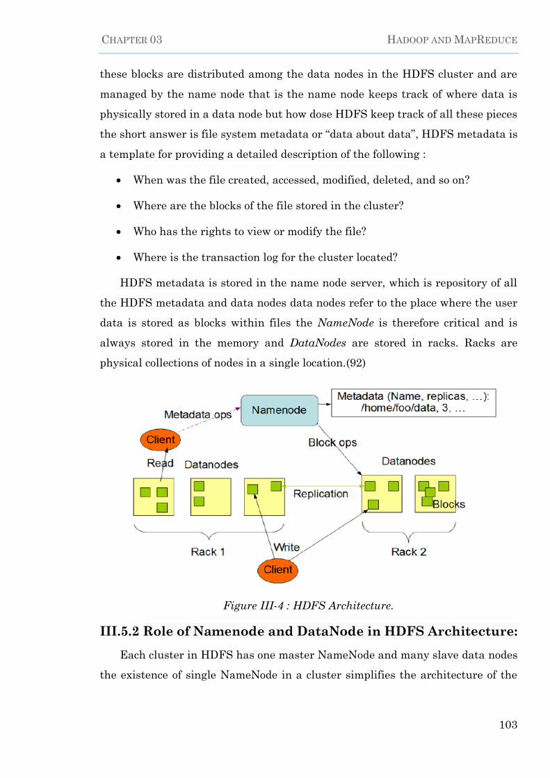
CHAPTER 03 HADOOP AND MAPREDUCE
103
these blocks are distributed among the data nodes in the HDFS cluster and are
managed by the name node that is the name node keeps track of where data is
physically stored in a data node but how dose HDFS keep track of all these pieces
the short answer is file system metadata or “data about data”, HDFS metadata is
a template for providing a detailed description of the following :
When was the file created, accessed, modified, deleted, and so on?
Where are the blocks of the file stored in the cluster?
Who has the rights to view or modify the file?
Where is the transaction log for the cluster located?
HDFS metadata is stored in the name node server, which is repository of all
the HDFS metadata and data nodes data nodes refer to the place where the user
data is stored as blocks within files the NameNode is therefore critical and is
always stored in the memory and DataNodes are stored in racks. Racks are
physical collections of nodes in a single location.(92)
Figure III-4 : HDFS Architecture.
III.5.2 Role of Namenode and DataNode in HDFS Architecture:
Each cluster in HDFS has one master NameNode and many slave data nodes
the existence of single NameNode in a cluster simplifies the architecture of the

CHAPTER 03 HADOOP AND MAPREDUCE
104
system because it acts a single arbitrator and repository for all HDFS metadata
as a result of the relatively low amount of metadata per file.
A NameNode: stores all of the metadata in the main memory,enabling a fast
random Manages all the file operations such as read/write create delete and
replicate data locks on the data nodes it also Manages the file system Namespace.
III.5.3 How NameNodes works:
The NameNode is vital to correct operation of the cluster hence to ensure the
availability of data, Secondary Name node is also available through a relationship
exists between the NameNode and the DataNodes they are loosely this allows the
cluster elements to add or subtract servers as the demand changes normally one
NameNode and possibly a data node run on one physical server in the rack while
other servers were data nodes only within the HDFS all the DataNode are
collected into a the rack the NameNode uses a rack ID to keep track of all the
DataNodes in the cluster the NameNode tracks the data on various DataNodes
that make up a complete file.
Figure III-5 : How NameNodes Works.
III.5.4 How DataNodes Works:
We know that in HDFS data is stored in multiple Data Node consequently
access to a file will require access to multiple Data Nodes, its benefit throughput
in two ways for one the Data Node, storing each HDFS data block in a separate
file on a local file system Not creating all files in the same directory of the native

CHAPTER 03 HADOOP AND MAPREDUCE
105
operating system and instead determines the optimal number of files per
directory and creates sub directories appropriately.
But how does Data Node and NameNode interact?
DataNodes constantly interact with the NameNode to check if there is
anything for them to do which alerts the NameNode about the availability of
DataNodes its also communicate among themselves to cooperate during normal
file system operations which is important as blocks for one file are likely to be
stored on multiple DataNodes.
DataNodes work by providing "heartbeat" messages to detect and ensure
connectivity between the NameNode and themselves when a heartbeat is no
longer detected the NameNode unmapped the DataNode from the cluster and
keeps on operating as though nothing has happened then when the heartbeat
returns or a new heartbeat appears it is added to the cluster.
Figure III-6 : How DataNodes Works.

CHAPTER 03 HADOOP AND MAPREDUCE
106
III.5.5 Rack Organization:
Data Notes that we have just discussed are organized within racks.
Racks are physical collections of machines in a single location using the
Hadoop rack awareness process the NameNode determines the rack ID that each
data node belongs to rack awareness also is an important characteristic of the data
storage in HDFS large HDFS instances run on a cluster of computers that is
usually spread across many racks network bandwidth and performance is usually
better between machines in the same rack than between machines in different
racks a simple policy is to place replicas on unique racks which not only prevents
losing data when entire rack is lost but also evenly distributes replicas in the
cluster in addition it also allows using bandwidth from multiple racks when
reading data an optimization of a rack aware policy is to use a number of racks
that is less than number of replicas to minimize global bandwidth consumption
and read latency.
Figure III-7 : Rack Organization.
III.5.6 How Data is stored in HDFS :
To understand how data is stored in HDFS, think of a file that contains all the
volumes of an encyclopedia with volume 1 being stored on server 1 volume 2 on
server 2 and so on if we were to equate this with the Hadoop world pieces of this
encyclopedia would be stored across the cluster which is a larger unit that is used
to organize and identify files on the disk. to reconstruct the entire encyclopedia

CHAPTER 03 HADOOP AND MAPREDUCE
107
your program would need blocks from every server in the cluster to achieve
availability if components fail HDFS replicates these smaller pieces on to
additional servers by default this redundancy offers multiple benefits.
The most obvious being higher availability therefore HDFS is so resilient that
these blocks are replicated throughout the cluster in case of a server failure.
Let us now see how this is translated to data storage in HDFS now we know
that HDFS is implemented as a block structured file system in which individual
files are broken into blocks of a fixed size and these are stored across clusters, each
data file is broken into equal size blocks of 64 MB and each block is stored in three
different DataNodes, this unique capability offers fault tolerant and faster
processing capabilities but how is this done.
The process of storing each block in replicates of three, ensures data
availability even if any one of the nodes becomes non-functional and thereby:
Enhancing the fault tolerance capabilities, the splitting of the file and equal
size blocks.
Ensures that all nodes perform at the same speed and efficiency.
Figure III-8 : Data Storage in HDFS.
III.5.6.1 Replication and Recovery:
File can become unavailable if any one of the machines is lost to avoid the
problem HDFS replicates each block across three machines by default, so the client

CHAPTER 03 HADOOP AND MAPREDUCE
108
is the HDFS user, it can read and write the data though calling the
API provided by HDFS. While in the read and write process, the client first
needs to obtain the metadata information from the NameNode, and then the
client can perform the corresponding read and write operations.(92)
III.5.7 Data Reading Process in HDFS:
The data reading process in HDFS is not difficult. It is similar to the
programming logic, which has created the object, i.e., calling the method and
performing the execution. The following section will introduce the reading
processing of the HDFS.(93)
Figure III-9 : HDFS Reading Process.
According to Figure III-9, there are six steps when the HDFS has the reading
process:
1. The client will generate a Distributed File System object of the HDFS class
library and uses the open() interface to open a file.
2. Distributed File System sends the reading request to the Namenode by
using the Remote Procedure Call Protocol to obtain the location address of the data
block. After the calculating and sorting the distance between the client and the
Datanode, the Namenode will return the location information of the data block to
the Distributed File System.

CHAPTER 03 HADOOP AND MAPREDUCE
109
3. After, the DistributedFileSystem has already received the distances and
address of the data block; it will generate an FSDataInputStream object instance
to the client. At the same time, the FSDataInputStream also encapsulates a
DFSInputStream object, which is responsible for saving the storing data blocks
and the address of the Datanode.
4. When everything gets ready, the client will call the read () method.
5. After receiving the calling method, the encapsulated DFSInputStream of
FSDataInputStream will choose the nearest Datanode to read and return the data
to the client.
6. When all the data has been read successfully, the DFSInputStream will be
in charge of closing the link between the client and the Datanode. While the
DFSInputStream is reading the data from the Datanode, it is hard to avoid the
failure that may be caused by network disconnection or node errors. When this
happens, DFSInputStream will give up the failure Datanode and select the
nearest Datanode. In the later reading process, the disfunctioning Datanode will
not be adopted anymore. It is observed that HDFS separates the index and data
reading to the Namenode and Datanode. The Namenode is in charge of the light
file index functions while the heavy data reading is accomplished by several
distributed Datanodes. This kind of platform can be easily adapted to the multiple
user access and huge data reading.
III.5.8 Data writing Process in HDFS:
The data writing process in HDFS is the opposite process of the reading but
the writing process is more complex. The following section will introduce the
writing process in HDFS briefly.

CHAPTER 03 HADOOP AND MAPREDUCE
110
Figure III-10 : HDFS Writing Process.
The structure of HDFS reading process is similar to the writing process. These
are the following seven steps:
1. The client generates a DistributedFileSystem object of the HDFS class
library and uses the create() interface to open a file.
2. DistributedFileSystem sends the writing request to the Namenode by using
the Remote Procedure Call Protocol (RPC). The Namenode will check if there is a
duplicate file name in it. After that, the client with writing authority can create
the corresponding records in the namespace. If an error occurrs, the Namenode
will return the IOException to the client.
3. After the DistributedFileSystem has received the successful return message
from the Namenode, it will generate a FSDataOutputStream object to the client.
In the FSDataOutputStream, there is an encapsulated DFSOutputStream object
which is responsible for the writing process. The client calls the write() method
and sends the data to the FSDataInputStream. The DFSOutputStream will put
the data into a data queue which is read by the DataStreamer. Before the real
writing, the DataStreamer needs to ask for some blocks and the suitable address
from the Datanode to store the data.

CHAPTER 03 HADOOP AND MAPREDUCE
111
4. For each data block, the Namenode will assign several Datanodes to store
the data block. For instance, if one block needs to be stored in three Datanodes.
DataStreamer will write the data block at the first Datanode, then the first
Datanode will pass the data block to the second Datanode, and the second one
passes to the third one. Finally, it will complete the writing data in the Datanode
chain.
5. After every Datanode has been written, Datanode will report to the
DataStreamer. Step4 and Step5 will be repeated until all the data has been
written successfully.
6. When all the data has been written, the client will call the close() method of
FSDataInputStream to close the writing operation.
7. Finally, the Namenode will be informed by the DistributedFileSystem that
all the written process has been completed. In the process of data writing, if one
Datanode makes error and causes writing failure, all the links between the
DataStreamer and the Datanode will be closed. At the same time, the failure node
will be deleted from the Datanode chain. The Namenode will notice the failure by
the returned packages and will assign a new Datanode to continue the processing.
As long as one Datanode is written successfully, the writing operation will regard
the process as completed.
III.5.9 Limitations of HDFS:
HDFS as the open source implementation of GFS is an excellent distributed
file system and has many advantages. HDFS was designed to run on the cheap
commodity hardware not on expensive machines. This means that the
probabilities of node failure are slightly high. To give a full consideration to the
design of HDFS, we may find that HDFS has not only advantages but also limits
for dealing with some specific problems. These limitations are mainly displayed in
the following aspects:
High Access Latency : HDFS does not fit fort requests which should be
applied in a short time. The HDFS was designed for the Big Data storage
and it is mainly used for it high throughput abilities. This may cost the high

CHAPTER 03 HADOOP AND MAPREDUCE
112
latency instead.Because HDFS has only one single Master system, all the
file requests need to be processed by the Master. When there is a huge
number of requests, there is inevitably has the delay. Currently, there are
some additional projects to address this limitation, such as using the Hbase
uses the Upper Data Management project to manage the data.
Poor small files performance : HDFS needs to use the Namenode to manage
the metadata of the file system to respond to the client and return the
locations so that the limitation of a file size is determined by the Namenode.
In general, each file, folder, and block need to occupy the 150 bytes’ space.
In other words, if there are one million files and each file occupies one block,
it will take 300MB space. Based on the current technology, it is possible to
manage millions of files. However, when the files extend to billions, the
work pressures on the Namenode is heavier and the time of retrieving data
is unacceptable.
Unsupported multiple users write permissions : in HDFS, one file just has
one writer because multiple users’ writer permissions are not supported yet.
The write operations can only be added at the end of the file not at the any
positions of the file by using the Append method.
We believe that, with the efforts of the developers of HDFS, HDFS will become
more powerful and can meet more requirements of the users.
III.6 MapReduce:
MapReduce is a programming model designed for processing large volumes of
data in parallel by dividing the work into a set of independent tasks. MapReduce
programs are written in a particular style influenced by functional
programming constructs, specifically idioms for processing lists of data. This
module explains the nature of this programming model and how it can be used to
write programs, which run in the Hadoop environment, MapReduce engine is a
high-performance parallel or distributed data processing implementation of the
MapReduce algorithm this means that it can be used to write programs that can

CHAPTER 03 HADOOP AND MAPREDUCE
113
process the large amounts of unstructured data by using a number of distributed
processors simultaneously.
III.6.1 MapReduce Functional Concept:
The MapReduce model is a combination of two capabilities in existing
functional computer languages Map and reduce the map function of MapReduce
distributes jobs tasks across a large number of systems it also handles the
placement of these tasks in a way that it balances the load manages recovery from
failures. The reducer function aggregates all the elements back together to provide
a result the map and reduce functions are a good choice for Big Data as they do
not modify the original data but create new data structures as their output.
Figure III-11 : How MapReduce Works.
III.6.2 Characteristics of MapReduce:
There are four main characteristics of the MapReduce:
Scheduling: In Map Reduce jobs are broken down into individual tasks for
the map and the reduce functions of the application the mapping is completed
before reducing can begin and the entire process is complete only when all the
reduced tasks have run successfully.
Synchronization: since more than one process is concurrently executed in
the cluster synchronization mechanisms must be in place this includes a function
called shuffle and sort, which collects and prepares all the mapped data for
reduction.

CHAPTER 03 HADOOP AND MAPREDUCE
114
Code /Data co-location: where code refers to the mapping functions the code
and data must be co-located or located on the same machine or node to ensure
effective processing.
Fault and error handling: most MapReduce engines have error handling,
fault tolerance mechanisms in place that recognize when something wrong, and
make the necessary correction.
III.6.3 The working process of MapReduce:
When to use big data efficiently it is necessary to access large amounts of input
data select relevant parts from it and to then compute something of value for
businesses from these parts all the while ensuring that the original data does not
get changed to ensure that this is done without human error an application needs
to perform these tasks, the MapReduce framework consists of a single master
which is called the job tracker and three slaves(see Figure III-12) , referred to as
task trackers the client application provide jobs to job tracker which in turn
submits or schedules the jobs to different task trackers these task trackers then
process the data the processed data also Known as map outputs is then is
forwarded to reduce tasks which integrates the data from different task trackers
and generates the final output MapReduce performs its tasks in a series of steps:
1. The input is split into multiple pieces of data.
2. The master and workers are created and the worker processes is executed
remotely.
3. The map worker uses the map function to extract relevant data, and then
generates a key-value pair for the extracted data.
4. The map worker uses the partitioning function to partition the data into R
regions.
5. The master now instructs the reduce workers to contact the map workers to
get the key/value data for their partition. The data received is sorted as per keys,
a process termed as the shuffle process.
6. After storing of the data the reduce function is called for every unique key,
and is used to write the output sent to file.

CHAPTER 03 HADOOP AND MAPREDUCE
115
7. When the reduce workers complete their work, the master transfers the
control to the user program.
Figure III-12 : MapReduce Procedure.
III.6.4 Limitations of MapReduce:
Although MapReduce is popular all over the world, most people still have
realized the limits of the MapReduce. The following are the four main limitations
of the MapReduce:
The bottleneck of Job Tracker:
The JobTracker should be responsible for jobs allocation, management, and
scheduling. In addition, it should also communicate with all the nodes to know the
processing status. It is obvious that the JobTracker which is unique in the
MapReduce, takes too many tasks. If the number of clusters and the submission
jobs increase rapidly, it will cause network bandwidth consumption. As a result,
the JobTracker will reach bottleneck and this is the core risk of MapReduce.
TaskTracker:
Because the jobs allocation information is too simple, the TaskTracker might

CHAPTER 03 HADOOP AND MAPREDUCE
116
assign a few tasks that need more sources or need a long execution time to the
same node. In this situation, it will cause node failure or slow down the processing
speed.
Jobs Delay:
Before the MapReduce starts to work, the TaskTracker will report its own
resources and operation situation. According to the report, the JobTracker will
assign the jobs and then the TaskTracker starts to run. Consequently, the
communication delay may make the JobTracker to wait too long so that the jobs
cannot be completed in time.
Inflexible Framework:
Although the MapReduce currently allows the users to define its own functions for
different processing stages, the MapReduce framework still limits the
programming model and the resources allocation.
III.7 YARN (Yet Another Resource Negotiator) :
In order to solve above limitations, the designers have put forward the next
generation of MapReduce: YARN (Yet Another Resource Negotiator) is Hadoop’
s cluster resource management System.
YARN was introduced in Hadoop 2 to improve the MapReduce
implementation, but it is general enough to support other distributed computing
paradigms as well. YARN provides APIs for requesting and working with cluster
resources, but these APIs are not typically used directly by user code. Instead,
users write to higher-level APIs provided by distributed computing frameworks,
which themselves are built on YARN and hide the resource management details
from the user. The situation is illustrated in Figure III-13, which shows some
distributed computing frameworks (MapReduce, Spark, and so on) running as
YARN applications on the cluster compute layer (YARN) and the cluster storage
layer (HDFS and HBase).(94)

CHAPTER 03 HADOOP AND MAPREDUCE
117
Figure III-13 : YARN Applications.
Given the limitations of MapReduce, the main purpose of YARN is to divide
the tasks for the JobTracker.
In YARN resources are managed by the ResourceManager and the jobs are
traced by the ApplicationMaster. The TaskTracker has become the NodeManager.
Hence, the global ResourceManager and the local NodeManager compose the data
computing framework. In YARN, the ResourceManager will be the resources
distributor while the ApplicationMaster is responsible for the communication with
the ResourceManager and cooperate with the NodeManager to complete the tasks.
III.7.1 YARN architecture:
Compared with the old MapReduce Architecture, it is easy to find out that
YARN is more structured and simple. Then, the following section will introduce
the YARN architecture:
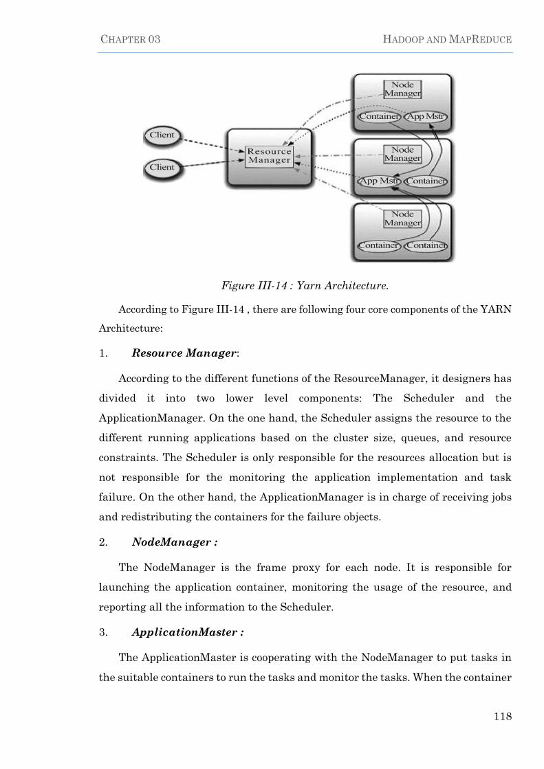
CHAPTER 03 HADOOP AND MAPREDUCE
118
Figure III-14 : Yarn Architecture.
According to Figure III-14 , there are following four core components of the YARN
Architecture:
1. Resource Manager:
According to the different functions of the ResourceManager, it designers has
divided it into two lower level components: The Scheduler and the
ApplicationManager. On the one hand, the Scheduler assigns the resource to the
different running applications based on the cluster size, queues, and resource
constraints. The Scheduler is only responsible for the resources allocation but is
not responsible for the monitoring the application implementation and task
failure. On the other hand, the ApplicationManager is in charge of receiving jobs
and redistributing the containers for the failure objects.
2. NodeManager :
The NodeManager is the frame proxy for each node. It is responsible for
launching the application container, monitoring the usage of the resource, and
reporting all the information to the Scheduler.
3. ApplicationMaster :
The ApplicationMaster is cooperating with the NodeManager to put tasks in
the suitable containers to run the tasks and monitor the tasks. When the container

CHAPTER 03 HADOOP AND MAPREDUCE
119
has errors, the ApplicationMaster will apply for another resource from the
Scheduler to continue the process.
4. Container :
In YARN, the Container is the source unit which is the available node splitting
the organization resources. Instead of the Map and Reduce source pools in
MapReduce, the ApplicationMaster can apply for any numbers of the Container.
Due to the same property Containers, all the Containers can be exchanged in the
task execution to improve efficiency.
III.7.2 Advantages of YARN:
Compared to the MapReduce, there are many advantages of the YARN
framework. There are four main advantages of YARN compared to the
MapReudce:
YARN greatly enhances the scalability and availability of the cluster by
distributing the tasks to the JobTracker. The ResourceManager and the
ApplicationMaster greatly relieves the bottleneck of the JobTracker and the safety
problems in the MapReduce.
In YARN, the ApplicationMaster is a customized component. That means
that the users can write their own program based on the programming model. This
makes the YARN more flexible and suitable for wide use.
YARN, on the one hand, supports the program to have a specific checkpoint.
It can ensure that the ApplicationMaster can reboot immediately based on the
status which was stored on HDFS. On the other hand, it uses the ZooKeeper on
the ResourceManager to implement the failover. When the ResourceManager
receives errors, the backup ResourceManager will reboot quickly. These two
measures improve the availability of YARN.
The cluster has the same Containers are the Reduce and Map pools in Map
Reduce. Once there is a request for resources, the Scheduler will assign the
available resources in the cluster to the tasks and regard the resource type. It will
increase the utilization of the cluster resources.

CHAPTER 03 HADOOP AND MAPREDUCE
120
III.8 Commercial distribution of Hadoop:
Apart from the aforementioned open source distribution of Hadoop which is
maintained by Apache, several other commercial distribution versions exist too,
each of them offers unique features to address big data challenges. Together these
distributions complete the ecosystem of Hadoop, Cloudera, Hortoworks, intel,
Greenplum,MapR,and AWS EMR are example of such distributions:
Hortonworks: Hortonworks data platform is a complete solution offering
not just data processing and management, but the enterprise spanning
security and governance.
MapR: this Apache Hadoop distribution claims to provide full data
protection, no single points of failure, improved performance, and dramatic ease
of use advantages.
Cloudera : Cloudera is seen by many people as the market leader in the
Hadoop space because it released the first commercial Hadoop distribution and it
is a highly active contributor of code to the Hadoop ecosystem, in addition to its
commercial distribution cloudera also maintain a free and open source version
which integrate the Hadoop core component , called CDH (Cloudera Distribution
with Hadoop), this will be discussed in detail in the next section as it is the
platform used for building the cluster and running the application subject of the
present thesis.
The Hadoop system can be extended with other technologies such as Dremel,
HPCC in deploying big data solutions, the diagram (See Figure III-) shows the
different tools and technologies that are based on Hadoop framework.
Together all the various elements mentioned above :(i) the Hadoop framework
(ii) the core components (iii) the commercial distributions and (iv) the related
technologies form a comprehensive toolset for targeting different big data
challenges.

CHAPTER 03 HADOOP AND MAPREDUCE
121
Figure III-15 : The Hadoop Ecosystem along with the Commercial Distributions.
III.8.1 Cloudera's Distribution with Hadoop (CDH):
Cloudera is an organization that has been working with Hadoop and its related
technologies for a few years now. It is an expert in the field of handling large
amounts of data using Hadoop and various other open source tools and projects. It
is one of the major contributors to several of the Apache projects. Over the years,
Cloudera has deployed several clusters for hundreds of its customers. It is
equipped with practical knowledge of the issues and details of real production
clusters. To solve these issues, Cloudera built CDH. In most distributed computing
clusters, several tools need to work Together to provide the desired output. These
tools are individually installed and are then configured to work well with each
other. This approach often creates problems as the tools are never tested together.
Also, the setup and configuration of these tools is tedious and prone to errors. CDH
solves this problem as it is packaged with thoroughly tested tools that work well
together in a single powerful distribution. Installation and configuration of the
various tools and components is more organized with CDH. CDH has everything
an enterprise needs for its big data projects. The components packaged into CDH
provide tools for storage as well as the computation of large Volumes of data. By
using CDH, an enterprise is guaranteed to have good support from the community

CHAPTER 03 HADOOP AND MAPREDUCE
122
for its Hadoop deployment.
Note that for this thesis we used CDH as our implementation platform.
Figure III-16 : CDH Main Admin Console “Cloudera Manager”.
III.8.1.1 Cloudera Manager:
Cloudera Manager is a web-browser-based administration tool to manage
Apache Hadoop clusters. It is the centralized command center to operate the entire
cluster from a single interface. Using Cloudera Manager, the administrator gets
visibility for each and every component in the cluster. A few of the important
features of Cloudera Manager are listed below:
It provides an easy-to-use web interface to install and upgrade CDH across
the cluster.
It provides an easy-to-use web interface to install and upgrade CDH across
the cluster.
Each node in the cluster can be assigned roles and can be configured
accordingly. It allows the starting and stopping of services across all nodes from a
single web interface.

CHAPTER 03 HADOOP AND MAPREDUCE
123
It provides complete information for each node, for example, CPU, memory
disk, and network statuses.
Cloudera Manager is available in the following two editions:
Cloudera Manager Standard (free).
Cloudera Manager Enterprise (licensed).
Cloudera Manager Standard Edition, though free, is a feature packed tool that
ca be used to deploy and manage Apache Hadoop clusters with no limitation on
the number of nodes. However, there are a few features that are not part of the
standard edition. These are as follows:
Lightweight Directory Access Protocol (LDAP) authentication.
Alerts via SNMP (Simple Network Management Protocol).
Operational reports and support integration.
Enhanced cluster statistics.
Disk quota management.
III.8.1.2 Understanding the Cloudera Manager Architecture:
The Cloudera Manager Server is the master service that manages the data model
of the entire cluster in a database. The data model contains information regarding
the services, roles, and configurations assigned for each node in the cluster.
The Cloudera Manager Server is responsible for performing the following
functions:
It communicates with Cloudera Manager Agents that are installed on each
node of the cluster and assigns tasks as well as checking the health of each agent
by monitoring its periodic heartbeats.
It provides an administrator web interface for the end user to perform
administrator operations.
It calculates and displays dashboards of the health for the entire cluster.

CHAPTER 03 HADOOP AND MAPREDUCE
124
It monitors the important parameters such as disk usage, CPU, and RAM
for each node in the cluster. It also allows full control on the Hadoop daemons
running on the cluster.
It manages the Kerberos credentials for the services running on the cluster.
Kerberos is the tool used to manage the authentication and authorization
requirements of the cluster.
It exposes a set of easy-to-use APIs that helps developers write their own
applications to interact with the Cloudera Manager Server.
The Cloudera Manager Agent is installed on each node of the cluster. It is
responsible for accepting tasks from the Cloudera Manager Server and performs
the starting and stopping of Hadoop daemons on its own node. It is also responsible
for gathering all system-level information and statistics and is relayed back to the
Cloudera Manager Server.
Figure III-17 depicts the cloudera manager architecture.
Figure III-17 : Cloudera Manager Architecture.(90)

CHAPTER 03 HADOOP AND MAPREDUCE
125
Key Points – Chapter 03 :
We Introduced the chapter by presenting the general History and a
concepts of Hadoop platform.
We described the main component that make up what is known by the
Hadoop ecosystem such as Hbase, Hive,Flume,……etc
We presented in detail the core component of Hadoop. HDFS its main
fault tolerant storage system that provides the basic structure and service
needed to support the core requirement of storage for Big Data and
MapReuce its computational engine for distributed computing.
We concluded the chapter by defining in brief the Cloudera Distribution
with CDH and its main management console Cloudera Manager, which
are used in conjunction as a platform for running the application.

CHAPTER 04 IMPLEMENTATION
126
Chapter IV:
Implementation

CHAPTER 04 IMPLEMENTATION
127
IV. Chapter 04
Implementation
Context:
As cited in previous chapters, frequent subgraph mining is one of the most
challenging tasks, this task has been highly motivated by the tremendously
increasing size of existing graph databases especially datasets in certain domains
such as bioinformatics, chemoinformatics and social networks. Due to this fact,
there is urgent need for efficient and scaling approaches for frequent subgraph
discovery, in this chapter, we study a novel iterative map reduce based method for
distributed large scale subgraph mining called FSM-H implemented with Hadoop.
The algorithm allows for using a different filtering and partitioning schemes, and
breaks the mining into different phases.
IV.1 Background:
In this work we are interested in frequent subgraph mining in a large graph
database containing small-medium size graphs:
Let, 𝐺 = {𝐺1, 𝐺2, …… . . , 𝐺𝑛} be a graph database, where each 𝐺𝑖 𝜖 𝐺, ∀ 𝑖 =
{1,…… , 𝑛} represents a labeled, undirected, simple (no multiple edges between a
pair of vertices), and connected graph. For a graph g, its size is defined as the
number of edges it contains. Now, 𝑡(𝑔) = { 𝐺𝑖 ∶ 𝑔 ⊆ 𝐺𝑖 𝜖 𝐺} , ∀𝑖 = {1…𝑛}, is the
support-set of the graph g (here the subset symbol denotes a subgraph relation).
Thus, 𝑡(𝑔) contains all the graphs in G that has a subgraph isomorphic to 𝑔. The
cardinality of the support-set is called the support of 𝑔. 𝑔 is called frequent if
𝑠𝑢𝑝𝑝𝑜𝑟𝑡 ≥ 𝜋𝑚𝑖𝑛 , where π𝑚𝑖𝑛 is predefined/user specified minimum
𝑠𝑢𝑝𝑝𝑜𝑟𝑡 (minsup) threshold. The set of frequent patterns are represented by 𝐹.
Based on the size (number of edges) of a frequent pattern, we can partition 𝐹 into
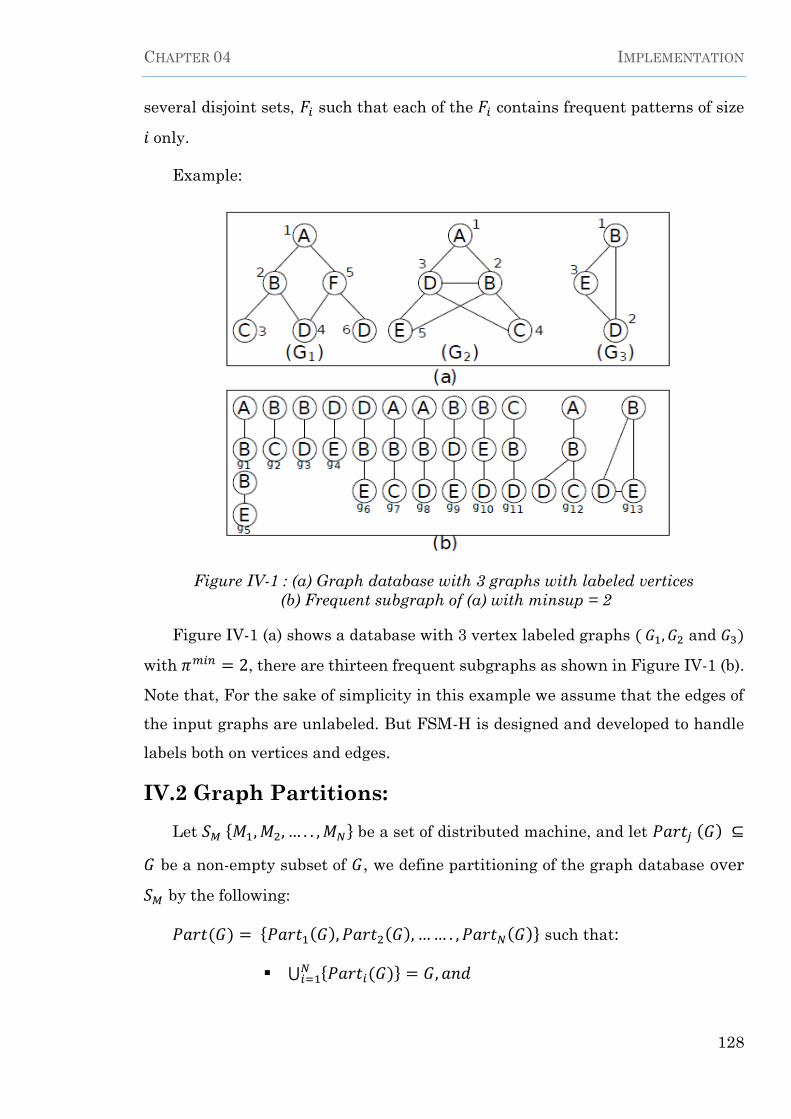
CHAPTER 04 IMPLEMENTATION
128
several disjoint sets, 𝐹𝑖 such that each of the 𝐹𝑖 contains frequent patterns of size
𝑖 only.
Example:
Figure IV-1 : (a) Graph database with 3 graphs with labeled vertices
(b) Frequent subgraph of (a) with minsup = 2
Figure IV-1 (a) shows a database with 3 vertex labeled graphs ( 𝐺1, 𝐺2 and 𝐺3)
with 𝜋𝑚𝑖𝑛 = 2, there are thirteen frequent subgraphs as shown in Figure IV-1 (b).
Note that, For the sake of simplicity in this example we assume that the edges of
the input graphs are unlabeled. But FSM-H is designed and developed to handle
labels both on vertices and edges.
IV.2 Graph Partitions:
Let 𝑆𝑀 {𝑀1, 𝑀2, … . . , 𝑀𝑁} be a set of distributed machine, and let 𝑃𝑎𝑟𝑡𝑗 (𝐺) ⊆
𝐺 be a non-empty subset of 𝐺, we define partitioning of the graph database over
𝑆𝑀 by the following:
𝑃𝑎𝑟𝑡(𝐺) = {𝑃𝑎𝑟𝑡1(𝐺), 𝑃𝑎𝑟𝑡2(𝐺), …… . , 𝑃𝑎𝑟𝑡𝑁(𝐺)} such that:
⋃ {𝑃𝑎𝑟𝑡𝑖(𝐺)} = 𝐺, 𝑎𝑛𝑑 𝑁𝑖=1

CHAPTER 04 IMPLEMENTATION
129
∀ 𝑖 ≠ 𝑗, 𝑃𝑎𝑟𝑡𝑖(𝐺) ∩ 𝑃𝑎𝑟𝑡𝑗(𝐺) = ∅.(13)
The above definition presents the general idea of partitioning graph datasets
over a set of machines, later in the chapter we define the heuristic employed by
FSM-H when doing so, for instance edge based of transaction based partitioning.
IV.3 Challenges:
Solving the task of frequent subgraph mining (FSM) on a distributed platform
like Map Reduce is challenging for various reasons. First, an FSM method
computes the support of a candidate subgraph pattern over the entire set of input
graphs in a graph dataset.
In a distributed platform, if the input graphs are partitioned over various
worker nodes like in our case. the local support of a subgraph in the respective
partition at a worker node is not much useful for deciding whether the given
subgraph is frequent or not. Also, local support of a subgraph in various nodes
cannot be aggregated in a global data structure, because, MapReduce
programming model does not provide any built-in mechanism for communicating
with a global state. Also, the support computation cannot be delayed arbitrarily,
as following Apriori principle, future candidate patterns can be generated only
from a frequent pattern.
IV.4 Contribution and Goals:
We study here an FSM-H algorithm which implements a distributed frequent
subgraph mining method over Map Reduce programming model. Given a graph
database, and a minimum support threshold, FSM-H generates a complete set of
frequent subgraphs. To ensure completeness, it constructs and retains all patterns
in a partition that have a non-zero support in the map phase of the mining, and
then in the reduce phase, it decides whether a pattern is frequent by aggregating
its support computed in other partitions from different computing nodes. To
overcome the dependency among the states of a mining process, FSM-H runs in
an iterative fashion, where the output from the reducers of iteration 𝑖 − 1 is used
as an input for the mappers in the iteration 𝑖. The mappers of iteration 𝑖 generate
candidate subgraphs of size 𝑖 (number of edge), and also compute the local support

CHAPTER 04 IMPLEMENTATION
130
of the candidate pattern. The reducers of iteration 𝑖 then find the true frequent
subgraphs (of size 𝑖) by aggregating their local supports. They also write the data
in disk that are processed in subsequent iterations.an external condition decides
the termination of an iteration (job).
Pseudo code for iterative MapReduce algorithm is presented in Figure VI-2 :
Figure IV-2 : Iterative MapReduce Algorithm
In the subsequent sections to come:
We introduce, FSM-H, a novel iterative MapReduce based frequent
subgraph mining algorithm, which is complete.
We describe the data structures that is used to save and consequently
propagate the states of the mining process over different iterations.
We empirically demonstrate the performance of FSM-H on synthetic as well
as real world large datasets.
IV.5 Method:
As mentioned earlier FSM-H is designed as an iterative MapReduce process
At the beginning of iteration 𝑖, FSM-H has at its disposal all the frequent
patterns of size 𝑖 − 1 (𝐹𝑖−1) and at the end of iteration 𝑖, it returns all the frequen
patterns of size 𝑖 (𝐹𝑖) Note that, in this work, the size of a graph is equal to the
number of edges it contains.
For a mining task if 𝐹 is the set of frequent patterns,FSM-H runs for a total of
𝑙 iterations, where 𝑙 is equal to the size of the largest graph in 𝐹.
To distribute a frequent subgraph mining (FSM) task, FSM-H partitions the
graph dataset 𝐺 = {𝐺𝑖}𝑖=1,…,𝑛 into 𝑘 disjoint partitions, such that each partition

CHAPTER 04 IMPLEMENTATION
131
contains roughly equal number of graphs; thus it mainly distributes the support
counting (discussed in details later) subroutine of a frequent pattern mining
algorithm. Conceptually, each node of FSM-H runs an independent FSM task over
a graph dataset which is 1 𝑘′⁄ th of the size of |𝐺|.Note that, 𝑘 is an important
parameter and details on how to choose it optimally is explained later In this
chapter.(85)
FSM algorithms in general are an adaptation of the baseline algorithm shown
in Figure II-23 far earlier in chapter 02, which actually runs in a sequential
machine, although just mentioned in chapter 02 below we provide more details on
this algorithm. Note that we do so with pattern growth approach as it is adopted
by FSM-H:
The pseudo-code The pseudo-code shown in Figure II-23 implements an FSM
algorithm that follows a typical candidate generation-and-test paradigm with
breadth-first candidate enumeration. In this paradigm, the mining task starts
with frequent patterns of size one (single edge patterns), denoted as 𝐹1 (Line0).
Then in each of the iterations of the while loop (Line 1-6), the method progressively
finds 𝐹2, 𝐹3 and so on until the entire frequent pattern set 𝐹 is obtained. If 𝐹𝑘 is
nonempty at the end of an iteration of the above while loop, from each of the
frequent patterns in 𝐹𝑘 the mining method creates possible candidate frequent
patterns of size 𝑘 + 1 (Line 2). These candidate patterns are represented as the set
𝐶. For each of the candidate patterns, the mining method computes the pattern’s
support against the dataset 𝐺 (Line 5). If the support is higher than the minimum
support threshold (𝑚𝑖𝑛𝑠𝑢𝑝), the given pattern is frequent, and is stored in the set
𝐹𝑘+1 (Line 6). Before support counting, the method also ensures that different
isomorphic forms of a unique candidate patterns are unified and only one such
copy is processed by the algorithm (Line 4). Once all the frequent patterns of size
𝑘 + 1 are obtained, the while loop in Line 1 to 7 continues. Thus each iteration of
the while loop obtains the set of frequent patterns of a fixed size, and the process
continues until all the frequent patterns are obtained. In Line 8, the FSM
algorithm returns the union of 𝐹 𝑖: 1 ≤ 𝑖 ≤ 𝑘 − 1.

CHAPTER 04 IMPLEMENTATION
132
Below, we provide a short description of each of the subroutines that are called
in the pseudo-code.
IV.5.1 Candidate Generation:
Given a frequent pattern (say, 𝑐) of size 𝑘, this step adjoins a frequent edge
(which belongs to 𝐹 1) with 𝑐 to obtain a candidate pattern d of size 𝑘 + 1. If 𝑑
contains an additional vertex then the added edge is called a forward edge,
otherwise it is called a back edge; the latter simply connects two of the existing
vertices of 𝑐. Additional vertex of a forward edge is given an integer id, which is
the largest integer id following the ids of the existing vertices of 𝑐; thus the vertex-
id stands for the order in which the forward edges are adjoined while building a
candidate pattern. 𝑐 is called the parent of 𝑑, and 𝑑 is a child of 𝑐, and based on
this parent-child relationship we can arrange the set of candidate patterns of a
mining task in a candidate generation tree (see figure IV-3) :
Note however that, if 𝑑 has 𝑘 + 1 edges, based on the order how its edges
have been adjoined, 𝑑 could have many different generation paths in a candidate
generation tree; FSM-H impose a restriction on the generation paths and only one
of which is considered valid, so that multiple copies of a candidate pattern are not
generated. Thus the candidate generation tree of an FSM-H can be unambiguously
defined. FSM-H also impose restriction on the extension nodes of the parent
pattern by allowing edge adjoining only with vertices on the right most path. Right
most path is the mechanism used in the so popular gSpan algorithm, so simply
put “right most vertex” (RMV) is the vertex with the largest id in a candidate
subgraph and “right most path” (RMP) is the shortest path from the lowest id
vertex to the RMV strictly following forward edges.(85)
Example: In the figure IV-3 below we define part of the candidate generation
tree of the FSM-H task that we defined in figure IV-1.

CHAPTER 04 IMPLEMENTATION
133
Figure IV-3 : Candidate generation subtree rooted under A-B.
Suppose we have explored all frequent level-1 patterns (𝑔1 to 𝑔4 in figure IV-1
– (b)) and we want to generate candidates from one of those patterns, namely 𝐴 −
𝐵. Figure IV-3 shows the part of the candidate generation subtree that is rooted
at the pattern 𝐴 − 𝐵. The nodes at the level 2 (root of the subtree is level 1) of this
subtree shows all possible candidate patterns of size 2 that are built by adjoining
the edge 𝐵 − 𝐶, 𝐵 − 𝐷, and 𝐵 − 𝐸, respectively, with the pattern 𝐴 − 𝐵. Note
that, all these candidate patterns are created by introducing a forward edge. At
this level, no candidate can be obtained by adding back edges because doing so will
create a multi-graph, which we do not allow. Also note, we do not extend 𝐴 − 𝐵
with another copy of 𝐴 − 𝐵 to create the pattern 𝐴 − 𝐵 − 𝐴 because none of the
database graphs in Figure IV-1 – (a) has multiple copies of the edge 𝐴 − 𝐵. Among
these three candidate patterns, the pattern 𝐴 − 𝐵 − 𝐸 is infrequent which is
denoted with the mark (𝐼) near the pattern. The remaining two patterns are
frequent, and they are subsequently extended to generate level-3 candidates. For
example, the pattern 𝐴 − 𝐵 − 𝐷 is extended with a back-edge to obtain the
triangle pattern 𝐴 − 𝐵 –𝐷 (all level-3 or level-4 candidates are not shown in this
figure). There are other important observations in Figure IV-3. First, the
extension of a pattern is only made on the rightmost path of that pattern. For
visual clarification, for each pattern we draw its rightmost path along a horizontal
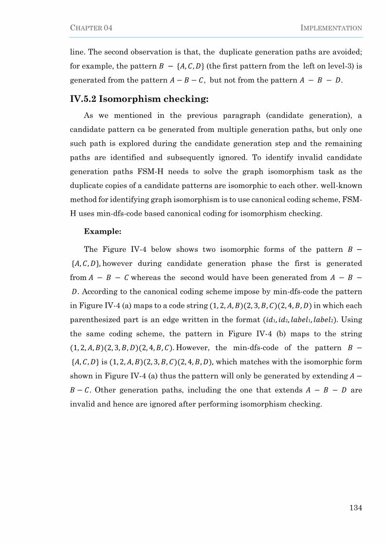
CHAPTER 04 IMPLEMENTATION
134
line. The second observation is that, the duplicate generation paths are avoided;
for example, the pattern 𝐵 − {𝐴, 𝐶, 𝐷} (the first pattern from the left on level-3) is
generated from the pattern 𝐴 − 𝐵 − 𝐶, but not from the pattern 𝐴 − 𝐵 − 𝐷.
IV.5.2 Isomorphism checking:
As we mentioned in the previous paragraph (candidate generation), a
candidate pattern ca be generated from multiple generation paths, but only one
such path is explored during the candidate generation step and the remaining
paths are identified and subsequently ignored. To identify invalid candidate
generation paths FSM-H needs to solve the graph isomorphism task as the
duplicate copies of a candidate patterns are isomorphic to each other. well-known
method for identifying graph isomorphism is to use canonical coding scheme, FSM-
H uses min-dfs-code based canonical coding for isomorphism checking.
Example:
The Figure IV-4 below shows two isomorphic forms of the pattern 𝐵 −
{𝐴, 𝐶, 𝐷}, however during candidate generation phase the first is generated
from 𝐴 − 𝐵 − 𝐶 whereas the second would have been generated from 𝐴 − 𝐵 −
𝐷. According to the canonical coding scheme impose by min-dfs-code the pattern
in Figure IV-4 (a) maps to a code string (1, 2, 𝐴, 𝐵)(2, 3, 𝐵, 𝐶)(2, 4, 𝐵, 𝐷) in which each
parenthesized part is an edge written in the format (𝑖𝑑1, 𝑖𝑑2, 𝑙𝑎𝑏𝑒𝑙1, 𝑙𝑎𝑏𝑒𝑙2). Using
the same coding scheme, the pattern in Figure IV-4 (b) maps to the string
(1, 2, 𝐴, 𝐵)(2, 3, 𝐵, 𝐷)(2, 4, 𝐵, 𝐶). However, the min-dfs-code of the pattern 𝐵 −
{𝐴, 𝐶, 𝐷} is (1, 2, 𝐴, 𝐵)(2, 3, 𝐵, 𝐶)(2, 4, 𝐵, 𝐷), which matches with the isomorphic form
shown in Figure IV-4 (a) thus the pattern will only be generated by extending 𝐴 −
𝐵 − 𝐶. Other generation paths, including the one that extends 𝐴 − 𝐵 − 𝐷 are
invalid and hence are ignored after performing isomorphism checking.

CHAPTER 04 IMPLEMENTATION
135
Figure IV-4 : Graph isomorphism.
IV.5.3 Support Counting:
Support counting of a graph pattern g is important to determine whether g is
frequent or not. To count g’s support we need to find the database graphs in which
g is embedded. One possible way to compute the support of a pattern without
explicitly performing the subgraph isomorphism test across all database graphs is
to maintain the occurrence-list (OL) of a pattern; such a list stores the embedding
of the pattern (in terms of vertex id) in each of the database graphs where the
pattern exists. When a pattern is extended to obtain a child pattern in the
candidate generation step, the embedding of the child pattern must include the
embedding of the parent pattern, thus the occurrence-list of the child pattern can
be generated efficiently from the occurrence list of its parent. Then the support of
a child pattern can be obtained trivially from its occurrence-list.
Example:
In Figure IV-5 we illustrate a simple scenario of support counting based on
occurrence list as it is performed by FSM-H. In the top three rows of Figure IV-5,
we show the OL of the pattern 𝐴 − 𝐵, 𝐵 − 𝐷 and 𝐵 − 𝐸. The Pattern 𝐴 – 𝐵 occurs
in Graph 𝐺1 and 𝐺2 in vertex pair (1, 2) and(1, 2), respectively; so its OL is:
1: [(1,2)]; 2: [(1,2)]. If we adjoin 𝐵 − 𝐷 with the pattern 𝐴 − 𝐵 and form the
pattern 𝐴 − 𝐵 − 𝐷, then we can construct the OL of 𝐴 − 𝐵 − 𝐷 (shown in 4th
row) by intersecting the OLs of 𝐴 − 𝐵 and 𝐵 − 𝐷. Note that, the intersection
considers both the graph ids and the vertex ids in the OLs. By counting the graph
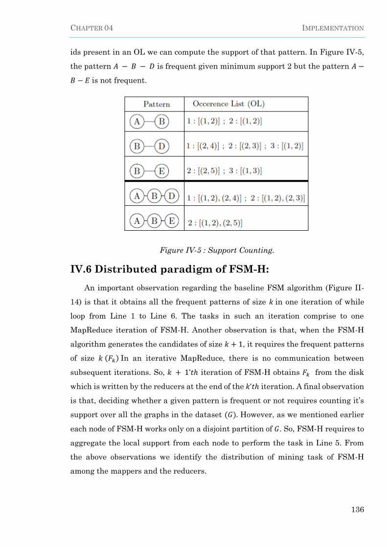
CHAPTER 04 IMPLEMENTATION
136
ids present in an OL we can compute the support of that pattern. In Figure IV-5,
the pattern 𝐴 − 𝐵 − 𝐷 is frequent given minimum support 2 but the pattern 𝐴 −
𝐵 − 𝐸 is not frequent.
Figure IV-5 : Support Counting.
IV.6 Distributed paradigm of FSM-H:
An important observation regarding the baseline FSM algorithm (Figure II-
14) is that it obtains all the frequent patterns of size 𝑘 in one iteration of while
loop from Line 1 to Line 6. The tasks in such an iteration comprise to one
MapReduce iteration of FSM-H. Another observation is that, when the FSM-H
algorithm generates the candidates of size 𝑘 + 1, it requires the frequent patterns
of size 𝑘 (𝐹𝑘) In an iterative MapReduce, there is no communication between
subsequent iterations. So, 𝑘 + 1’𝑡ℎ iteration of FSM-H obtains 𝐹𝑘 from the disk
which is written by the reducers at the end of the 𝑘’𝑡ℎ iteration. A final observation
is that, deciding whether a given pattern is frequent or not requires counting it’s
support over all the graphs in the dataset (𝐺). However, as we mentioned earlier
each node of FSM-H works only on a disjoint partition of 𝐺. So, FSM-H requires to
aggregate the local support from each node to perform the task in Line 5. From
the above observations we identify the distribution of mining task of FSM-H
among the mappers and the reducers.

CHAPTER 04 IMPLEMENTATION
137
IV.6.1 Pseudo code for the mapper:
Figure IV-6 shows the pseudo-code of a mapper. The argument 𝐹𝑘𝑝
represents
the set of 𝑠𝑖𝑧𝑒 − 𝑘 frequent subgraph having non-zero support in a specific
partition 𝑝. The mapper reads it from Hadoop Distributed FileSystems (HDFS).
Each pattern (𝑠𝑎𝑦 𝑥) in 𝐹𝑘𝑝
is read as a key-value pair. The key is the min-dfs-code
of the pattern (𝑥.𝑚𝑖𝑛 − 𝑑𝑓𝑠 − 𝑐𝑜𝑑𝑒) and the value is a pattern object (𝑥. 𝑜𝑏𝑗); here
“object” stands for its usual meaning from the object oriented programming. This
pattern object contains all the necessary information of pattern i.e., its support,
neighborhood lists, and occurrence list within partition 𝑝. It also contains
additional data structure that are used for facilitating candidate generation from
this pattern in the same partition. We will discuss the pattern object in details in
a later section.
Figure IV-6 : Mapper of distributed FSM-H Algorithm.
The mapper then generates all possible candidates of size 𝑘 + 1 (Line 1) by
extending each of the patterns in 𝐹𝑘𝑝
. For each of the generated candidates (𝑠𝑎𝑦, 𝑐),
the mapper performs isomorphism checking to confirm whether 𝑐 is generated
from a valid generation path; in other words, it tests whether 𝑐 passes the min-
dfs-code based isomorphism test (Line 3). For successful candidates, the mapper
populates their occurrence list (Line 4) over the database graphs in the partition
𝑝. If the occurrence list of a candidate pattern is non-empty, the mapper constructs
a keyvalue pair, such as, (𝑐.𝑚𝑖𝑛 − 𝑑𝑓𝑠 − 𝑐𝑜𝑑𝑒, 𝑐. 𝑜𝑏𝑗) and emits the constructed pair
for the reducers to receive (Line6).

CHAPTER 04 IMPLEMENTATION
138
IV.6.2 Pseudo code for the reducer:
shows the pseudo code for a reducer in distributed frequent subgraph mining.
The reducer receives a set of key-value pairs, where the key is the min-dfs-code of
a pattern namely 𝑐.𝑚𝑖𝑛 − 𝑑𝑓𝑠 − 𝑐𝑜𝑑𝑒 and the value is a list of 𝑐. 𝑜𝑏𝑗’𝑠 constructed
from all partitions where the pattern 𝑐 has a non-zero support.
Figure IV-7 : Reducer of distributed FSM-H Algorithm.
The Reducer then iterates (Line 1) over every 𝑐. 𝑜𝑏𝑗 and from the length of the
occurrence list of each 𝑐. 𝑜𝑏𝑗 it computes the aggregated support of 𝑐. If the
aggregated support is equal or higher than the minimum support threshold (Line
3), the reducer writes each element in the list paired with the 𝑚𝑖𝑛 − 𝑑𝑓𝑠 − 𝑐𝑜𝑑𝑒 of
𝑐 in HDFS for the mappers of the next iteration.
IV.7 Execution flow of FSM-H:
The Figure IV-8 below illustrates the execution flow of FSM-H. The execution
starts from the mappers as they read the key-value pair of size 𝑘 patterns in
partition 𝑝 from the HDFS. As shown in the Figure IV-8, the mappers generate
all possible 𝑘 + 1 − 𝑠𝑖𝑧𝑒 candidate patterns and perform the isomorphism checking
within partition 𝑝. For a pattern of size 𝑘 + 1 that passes the isomorphism test and
has a non-zero occurrence, the mapper builds its key-value pair and emits that for
the reducers. These key-value pairs are shuffled and sorted by the key field and
each reducer receives a list of values with the same key field. The reducers then
compute the support of the candidate pattern by aggregating the support value
computed in the partitions where the respective pattern is successfully extended.
If a pattern is frequent, the reducer writes appropriate key-value pairs in the
HDFS for the mappers of the next iteration. If the number of frequent 𝑘 + 1 size
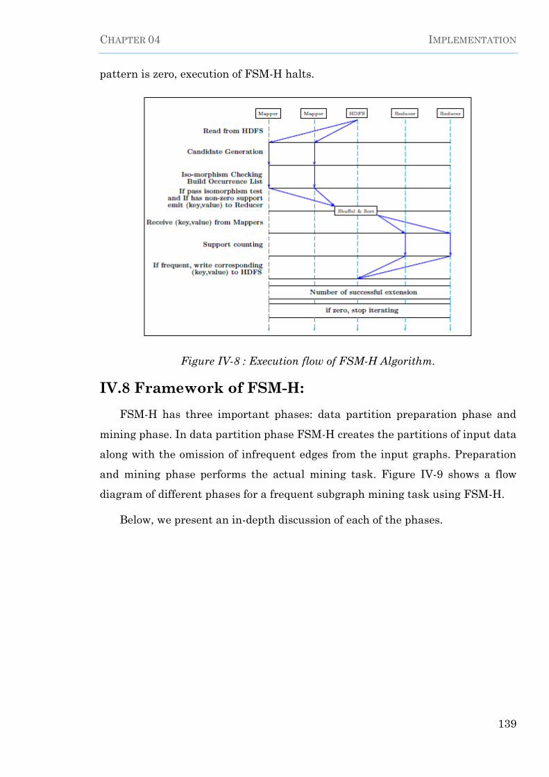
CHAPTER 04 IMPLEMENTATION
139
pattern is zero, execution of FSM-H halts.
Figure IV-8 : Execution flow of FSM-H Algorithm.
IV.8 Framework of FSM-H:
FSM-H has three important phases: data partition preparation phase and
mining phase. In data partition phase FSM-H creates the partitions of input data
along with the omission of infrequent edges from the input graphs. Preparation
and mining phase performs the actual mining task. Figure IV-9 shows a flow
diagram of different phases for a frequent subgraph mining task using FSM-H.
Below, we present an in-depth discussion of each of the phases.

CHAPTER 04 IMPLEMENTATION
140
Figure IV-9 : Framework of FSM-H.
IV.8.1 Data partition Phase:
In data partition phase, FSM-H splits the input graph dataset (𝐺) into many
partitions. One straightforward partition scheme is to distribute the graphs so
that each partition contains the same number of graphs from 𝐺. This works well
for most of the datasets. However, for datasets where the size (edge count) of the
graphs in a dataset vary substantially, FSM-H offers another splitting option in
which the total number of edges aggregated over the graphs in a partition are close
to each other. In experiment section, we show that the latter partition scheme has
a better runtime performance as it improves the load balancing factor of a
MapReduce job. For FSM-H, the number of partition is also an important tuning
parameter. In experiment section, we show that for achieving optimal
performance, the number of partitions for FSM-H should be substantially larger
than the number of partitions in a typical MapReduce task. During the partition

CHAPTER 04 IMPLEMENTATION
141
phase, input dataset also goes through a filtering procedure that removes the
infrequent edges from all the input graphs. While reading the graph database for
partitioning, FSM-H computes the support-list of each of the edges from which it
identifies the edges that are infrequent for the given minimum support threshold.
Example:
For the graph dataset in Figure IV-1, for a minimum support threshold of 2,
the edges 𝐴 − 𝐵, 𝐵 − 𝐶, 𝐵 − 𝐷, 𝐷 − 𝐸 and 𝐵 − 𝐸 are frequent and the remaining
edges are infrequent. Now suppose FSM-H makes two partitions for this dataset
such that the first partition contains 𝐺1, and the second partition contains 𝐺2 and
𝐺3.While making these partitions FSM-H filters the infrequent edges. Figure IV-
10 shows the partitioning where the infrequent edges are stripped off from the
database graphs.
Figure IV-10 : Input dataset after partition and filtering phase.
IV.8.2 Preparation Phase:
The mappers in this phase prepare some partition specific data structures
such that for each partition there is a distinct copy of these data structures. They
are static for a partition in the sense that they are same for all patterns generated
from a partition. The first of such data structure is called 𝑒𝑑𝑔𝑒 − 𝑒𝑥𝑡𝑒𝑛𝑠𝑖𝑜𝑛 − 𝑚𝑎𝑝,
which is used for any candidate generation that happens over the entire mining
session. It stores the possible extension from a vertex considering the edges that
exists in the graphs of a partition. For example, the graphs in partition two have
edges such as 𝐵 − 𝐷,𝐵 − 𝐶, 𝐵 − 𝐴, and 𝐵 − 𝐸. So, while generating candidates, if 𝐵
is an extension stub, the vertex 𝐴, 𝐶, 𝐷 or 𝐸 can be the possible vertex label of the

CHAPTER 04 IMPLEMENTATION
142
vertex that is at the opposite end of an adjoined edge. This information is stored
in the 𝑒𝑑𝑔𝑒 − 𝑒𝑥𝑡𝑒𝑛𝑠𝑖𝑜𝑛 − 𝑚𝑎𝑝 data structure for each of the vertex label that exist
in a partition. The second data structure is called 𝑒𝑑𝑔𝑒 − 𝑂𝐿, it stores the
occurrence list of each of the edges that exist in a partition; FSM-H use it for
counting the support of a candidate pattern which is done by intersecting the OL
of a parent pattern with the OL of an adjoint edge.
Example:
Figure IV-11 (a) and Figure IV-11 (b) shows these data structures for the
Partition 1 and 2 defined in Figure IV-10. In partition 1, the edge-extension choice
from a vertex with label 𝐷 is only 𝐵 (shown as 𝐷 ∶ (𝐵)), as in this partition 𝐵 − 𝐷
is the only frequent edge with a 𝐵 vertex. On the other hand, the corresponding
choice for partition 2 is 𝐵 and 𝐸 (shown as, 𝐷 ∶ (𝐵; 𝐸)), because in partition 2 we
have two edges, namely 𝐵 − 𝐷 and 𝐷 − 𝐸 that involve the 𝐷 vertex. In partition
1, the edge 𝐵 − 𝐷 occurs in 𝐺1 at vertex 𝑖𝑑 (2, 4); on the other hand in partition 2,
the same edge occurs in 𝐺2 and 𝐺3at vertex 𝑖𝑑 (2, 3) and (1, 2), respectively. This
information is encoded in the 𝑒𝑑𝑔𝑒 − 𝑂𝐿 data structures of these partitions as
shown in this figure.
Figure IV-11 : The static data structures and A-B-C pattern object in partition 1
and 2 (a) Edge-extension-map (b) Edge-OL (c) and (d) A-B-C Pattern object.

CHAPTER 04 IMPLEMENTATION
143
The mappers in the preparation phase also start the mining task by emitting
the frequent single edge patterns as key-value pair. Note that, since the partition
phase have filtered out all the infrequent edges, all single edges that exist in any
graph of any partition is frequent. As we mentioned earlier the key of a pattern is
its 𝑚𝑖𝑛 − 𝑑𝑓𝑠 − 𝑐𝑜𝑑𝑒 and the value is the pattern object.
Each pattern object has four essential attributes: (a) 𝑂𝑐𝑐𝑢𝑟𝑟𝑒𝑛𝑐𝑒 𝐿𝑖𝑠𝑡 (𝑂𝐿) that
stores the embedding of the pattern in each graph in the partition, (b) 𝑅𝑖𝑔ℎ𝑡 −
𝑀𝑜𝑠𝑡 − 𝑃𝑎𝑡ℎ (c) 𝑉𝑆𝐸𝑇 that stores the embedding of the Right Most Path in each
graph in the partition, and (d) 𝑠𝑢𝑝𝑝𝑜𝑟𝑡 value. Mappers in the preparation phase
compute the 𝑚𝑖𝑛 − 𝑑𝑓𝑠 − 𝑐𝑜𝑑𝑒 and create the pattern object for each single-edge
patterns. While emitting a key-value pair to a reducer, the mappers also bundle
the static data structures, 𝑒𝑑𝑔𝑒 − 𝑒𝑥𝑡𝑒𝑛𝑠𝑖𝑜𝑛 − 𝑚𝑎𝑝 and 𝑒𝑑𝑔𝑒 − 𝑂𝐿 with each of the
pattern object. FSM-H uses Java serialization to convert these objects in to byte
stream while sending them as value in a key-value pair. The reducers of this phase
actually do nothing but writing the input key-value pairs in HDFS since all the
single length patterns that the mappers send are frequent. In Figure IV-9, the
second block portrays the preparation phase.
Example:
Figure IV-11 (c) and IV-11 (d) exhibits the 𝑃𝑎𝑡𝑡𝑒𝑟𝑛 object along with their
attributes for the pattern 𝐴 − 𝐵 − 𝐶 in partition 1 and 2, respectively. The
attribute 𝑂𝐿 records the occurrence of this pattern in the corresponding database
graphs; if a pattern has multiple embeddings in a database graph all such
embeddings are stored. 𝑅𝑖𝑔ℎ𝑡 − 𝑀𝑜𝑠𝑡 − 𝑃𝑎𝑡ℎ records the id of the 𝑟𝑖𝑔ℎ𝑡 − 𝑚𝑜𝑠𝑡 −
𝑝𝑎𝑡ℎ vertices in the pattern object and 𝑉𝑆𝐸𝑇 stores the corresponding ids in the
database graphs. Like 𝑂𝐿, 𝑉𝑆𝐸𝑇 is also a set and it stores information for multiple
embedding if it applies. Finally, Support stores the support value of the pattern.
In the following discussion, we use ♣ and ♠ to denote a pattern object from
partition 1 (𝐺1) and 2 (𝐺2, 𝐺3), respectively. For example, ♠𝑎𝑏𝑐identifies the pattern
𝐴 − 𝐵 − 𝐶 from partition 2 as shown in Figure IV-11 (d).

CHAPTER 04 IMPLEMENTATION
144
IV.8.3 Mining Phase:
In this phase, mining process discovers all possible frequent subgraphs
through iteration. Preparation phase populates all frequent subgraphs of size one
and writes it in the distributed file system. Iterative job starts by reading these
from HDFS. Each of the mappers of an ongoing iteration is responsible for
performing the mining task over a particular chunk of the data written in HDFS
by the preparation phase. The map function of mining phase reconstructs all the
static data structures that are required to generate candidate patterns from the
current pattern. Using the static data structures and the pattern object, the
mappers can independently execute the subroutine that is shown in Figure IV-6.
The reducers in this phase simply execute the routine in Figure IV-7.
Example:
The figure IV-12 below provides a detail walk-through of a MapReduce job in
iteration phase with respect to the partitioned toy dataset mentioned in Figure IV-
10. Figure IV-12 (a) and (b) indicates the key-value pairs for pattern 𝐴 − 𝐵 from
partition 1 and 2. Suppose these key-value pairs are feed as input for Mapper 1
and Mapper 2 in Figure IV-12. The mappers first extract all data structures from
the value field of key-value pair including the partition-specific static data
structures (𝑆𝐷𝑆 in Figure IV-12) such as 𝑒𝑑𝑔𝑒 − 𝑒𝑥𝑡𝑒𝑛𝑠𝑖𝑜𝑛 − 𝑚𝑎𝑝 and 𝑒𝑑𝑔𝑒 − 𝑂𝐿.
Then they perform the steps mentioned in Figure IV-6. Figure IV-12 (c) and (d)
show the key-value pairs of 𝐴 − 𝐵 − 𝐶 that are generated by Mapper 1 and Mapper
2 by extending the pattern 𝐴 − 𝐵. The Reducers collect all the values for a key and
compute the support of the pattern by adding the supports from individual
partitions. In this example, the support of the pattern 𝐴 − 𝐵 − 𝐶 is 2; since
𝑚𝑖𝑛𝑠𝑢𝑝 = 2, this pattern is frequent. Reducers then write the key-value pairs
corresponding to the pattern 𝐴 − 𝐵 − 𝐶 in HDFS.

CHAPTER 04 IMPLEMENTATION
145
Figure IV-12 : One iteration of the mining phase of FSM-H with respect to pattern
A-B.
IV.9 Hadoop Pseudo Code:
In this section, we present the pseudo code of each phase using the syntax of
Hadoop framework. Figure IV-13, IV-14 and IV-15 demonstrate data partitioning,
preparation and mining phase, respectively. In Line 3 and 4 of Figure IV-13, FSM-
H performs the filtering and partitioning of the input dataset and writes each
partition and write in the HDFS.
Figure IV-13 : Data partitioning Phase.
In line 1-7 of Figure IV-14 the mappers generate static data structure along
with emit key-value pair of all single length pattern to reducer. Since all patterns
are frequent, Reducers just relay the input key, value pair to the output file in
HDFS.

CHAPTER 04 IMPLEMENTATION
146
Figure IV-14 : Preparation Phase.
In Line 1-3 of Mapper mining function in Figure IV-15, the mappers
reconstruct the pattern object of size 𝑘 a long with the static data structures and
generates the candidates from the current pattern. In Line 4-9, the mappers
iterate over all possible candidates of size 𝑘 + 1 and on success in isomorphism
and occurrence list test mappers emit the key-value pair for the reducer. Reducer
mining function computes the aggregate support (Line 2) of the pattern and if the
pattern is frequent, reducers write back the key, value pairs to HDFS for the
mappers of the next iteration.

CHAPTER 04 IMPLEMENTATION
147
Figure IV-15 : Mining Phase.
IV.10 Implementation Details:
We used Cloudera’s open source Distribution with Hadoop CDH 15-4, that
include Hadoop version 2-6-0, as a platform for running the application. The
baseline mining algorithm is written in java, as well as the map and the reduce
function for both the preparation and the mining phases. A custom input reader
is used instead of the default ones that came built-in with Hadoop.
To improve the execution time data is compressed when written to HDFS. we
used global counters provided by Hadoop to monitor and track the stopping point
of the iterative mining task.
IV.10.1 Map reduce job configuration:
Success of the job depends on the accurate configuration of it, and since the
type of the value that is read by a mapper and emit by the reducer is ByteWritable,
FSM-H sets the input and output format of each job as SequenceFileInputFormat

CHAPTER 04 IMPLEMENTATION
148
and SequenceFileOutputFormat respectively. Another job property, named
mapred.task.timeout also need to be set properly for better execution of FSM-
H. This parameter controls the duration for which the master node waits for a
data node to reply. If the mining task that FSM-H commence is computationally
demanding, the default timeout which is 10 minutes may not be enough. To be on
the safe side, FSM-H sets the timeout of the job to 5 hours (300 minutes). FSM-H
also sets the mapred.output.compress property to true. This configuration lets
the output of a MapReduce job to be compressed which eventually decreases
network load and improves the overall execution time. The codec that is used for
compression is BZip2Codec instead of the default one. BZip2Codec is shipped
with Hadoop. FSM-H also increases the heap size of a job using
mapred.child.java.opts property. The same configuration is used for both
the preparation and mining phase of FSM-H.
A list of some of the main configuration options that may enhance the
performance of the execution of jobs could be found in the appendix.

CHAPTER 04 IMPLEMENTATION
149
Key Points – Chapter 04 :
We introduced the chapter by defining the general formulation of FSM
problem where the input data is a database containing small to medium
sized transactions (graphs).
We highlighted the theoretic approaches adopted along with the different
data structures that is maintained by FSM-H in order to perform
candidate generation, isomorphism checking and support counting.
We highlighted the pseudo code for the mapper and the reducer of FSM-
H with respect to a configuration where we have a fully distributed
system.
We presented the general framework and execution flow of FSM-H for
instance partition, preparation and mining phases.
We concluded the chapter by presenting some tuning parameter that
once configured allow for best execution of the jobs.
CHAPTER 05 EXPERIMENTS AND RESULTS
150
Chapter V:
Experiments and Results

CHAPTER 05 EXPERIMENTS AND RESULTS
151
V. Chapter 05:
Experiments and Results
V.1 Experiments:
In this Section we present experimental results that demonstrate the
performance of FSM-H for solving frequent subgraph mining task where we have
a graph database containing a collection of small – to – medium sized graphs.
We have done several experiments on real datasets, taking into account a
variation of multiple factors (number of data nodes, number of mappers, reducers,
…. etc.).
For each test results we analyses it and demonstrate the efficiency of FSM-H.
V.2 Experimental setup:
V.2.1 Datasets:
In chemistry graphs can represent different chemical objects: molecules,
reactions, crystals, polymers, clusters, etc. The common feature of chemical
systems is the presence of sites and connections between them. Sites may be atoms,
electrons, molecules, molecular fragments, groups of atoms, intermediates,
orbitals, etc. The connections between sites may represent bonds of any kind,
bonded and no bonded interactions, elementary reaction steps, rearrangements,
van der Waals forces, etc. Chemical systems may be depicted by chemical graphs
using a simple conversion rule:
Site vertex
Connection edge
A special class of chemical graphs are molecular graphs. Molecular graphs are
chemical graphs which represent the constitution of molecules. They are also
called constitutional graphs. In these graphs vertices correspond to individual
atoms and edges to chemical bonds between them.

CHAPTER 04 IMPLEMENTATION
152
So as input we use six real-world graph datasets which are taken from an
online source that contains graphs extracted from the PubChem website.
PubChem is an open chemistry database at the National Institutes of Health
(NIH). It provides information on biological activities of small molecules and the
graph datasets from PubChem represent atomic structure of different molecules.
Table V-1: highlight some statistics about these real world graph datasets:
Table V-1 : statistics of real life graph datasets.
Name of Transaction
Graph dataset.
Assay
ID
# Transactions
(Graphs)
Tumor Description Average size
of each graph
SN12C 145 40004 Renal 27.7
NCI-H23 1 40353 Non-small Cell
Lung
28.6
OVCAR-8 109 40516 Ovarian 28.1
SF-295 47 40271 Central Nerv syst 28.0
YEAST 167 79601 Yeast Anticancer 22.8
Name of Transaction Graph dataset: refer to the name of the anticancer
screen test, the graphs in each dataset represent chemical compounds that
were exposed to some test cell lines in laboratory.
Assay id: refers to the bioassay ID as it is identified in the PubChem
database.
# Transactions (Graphs): represent the number of transactions (graphs)
in each dataset.
Tumor description: Refers to the cancer type that these chemical
compounds (graphs in our case) were tested against.
Average size of each graph: refers to the average size (number of edges)
of graphs in each dataset.
Rq: the graphs in each dataset (chemical compounds) are grouped into
two categories depending on the bioactivity outcome:

CHAPTER 04 IMPLEMENTATION
153
Active: means that the tested chemical molecule (compound)
has an active outcome with respect to the objective of the test
which is in general the growth inhibition of the tumor in the
cells tested.
Inactive: means that the tested chemical compound didn’t
present any activity against the cell that it was exposed to.
Performing frequent subgraph mining against these chemical graph datasets
could reveal the main component (frequent subgraph: frequent compounds) that
are shared amongst them, which could be of huge value because these frequent
patterns help in the fabrication of drugs for the treatment of malignant,
or cancerous diseases.
V.2.1.1 Graph representation in machine:
Each graph from the graphs mentioned in Table V-1 and their mappings to
chemical structures are represented and stored in text files as captured in the
figure V-1 below:
(a): represent a graph (a chemical compound):
o t # 0: refers to transaction number 0 (first graph in the dataset).
o v 0 0: vertex 0 has a label 0 (labels here correspond to atoms
example: O, C, H, Br, …. etc.
(a) (b)
Figure V-1 : (a) Exerpt from the yeast graph dataset file.
(b) Exerpt from the mapping text file that correspond to yeast graph dataset.

CHAPTER 04 IMPLEMENTATION
154
o e 1 13 1: there is an edge between vertex 0 and vertex 13 that has
a label of 1.
o Labels can be represented by an integer 1 or 2, labels define the type
of the bond that exist between atoms(vertexes)
1: define simple bond between elements(atoms).
2: define double bonds between two elements (atoms)
(b): correspond to an excerpt from the file mapping.txt that store the
mapping of chemical elements(atoms) to an integer id: for example, C 3 in
the file means that C (carbon) has an integer id of 3, so whenever we find
in the graph dataset a vertex with label 3 we know that it represents C
(carbon) and from this observation we can define the chemical structure
that we are dealing with, that is represented here as a transaction.
It is important to note here that mapping.txt does not include the Hydrogen
atom and thus the type of graphs that we are dealing with are called
“hydrogen-suppressed molecular graphs”, example of such graphs are
presented in the example below.
Example:
Figure V-2 : Example of two hydrogen-suppressed molecular graphs depicting
butane and cyclobutane.
.
CHAPTER 04 IMPLEMENTATION
155
V.2.2 Implementation platform:
We used Cloudera’s distribution with Hadoop CDH 15-4, that include Hadoop
version 2.6.0 as a platform for running the program, note also that all experiments
were conducted on real Cluster composed of four nodes, running each of them
Cent-OS version 7.0.
Each of the four nodes is equipped with 12 Core Xeon, 2.5 Ghz CPU and having
125 Gb of memory and 1TB or storage space.
Note that for each of the tests (see next section) we keep each partition with
approximately 100 graphs. And balances the graphs in each of them to be having
approximately the same number of edges.
V.3 Tests and Evaluations:
V.3.1 Runtime of FSM-H for different minimum support:
In this experiment, we analyze the runtime of FSM-H for varying minimum
support threshold. We conduct this experiment for the real world datasets
mentioned above. Here we fix the number of data nodes to 4 and keep 100
transactions for each partition. and we observe the running time of FSM-H for a
minimum support threshold that vary between 50 and 120 (with values 50, 70, 90
and 120 respectively). In Figure V-3 (a-e) we show the result. As expected, the
runtime decreases as minimum support threshold increases. In figure V-4(a-d), we
show the overall running time of FSM-H distributed over “Map” and ”Reduce“
phases. We pick “yeast” and “SN12C” dataset for this experimentation. In all cases
(different supports), the “Reduce” phase takes large time to execute than the
”Map” phase. More precisely, the running time of “Reduce“ phase is approximately
70% of overall running time.

CHAPTER 04 IMPLEMENTATION
156
Figure V-3 : Line Plot Showing the relationship between the minimum support
threshold and the running time n minutes for (a) Yeast, (b) SN12C (c) OVCAR-8
(d) NCI-H23 and (e) SF295.
0
20
40
60
80
100
50 70 90 120
Ru
nti
me
(in
min
ute
s)
Support
SN-12C
0
20
40
60
80
50 70 90 120
Ru
nti
me
(in
min
ute
s)
Support
Yeast
0
20
40
60
80
100
120
50 70 90 120R
un
tim
e (i
n m
inu
tes)
Support
NCI-H23
0
20
40
60
80
100
50 70 90 120
Ru
nti
me
(in
min
ute
s)
Support
OVCAR-8
0
20
40
60
80
100
50 70 90 120
Ru
nti
me
(in
min
ute
s)
Support
SF295
(a) (b)
(c) (d)
(e)
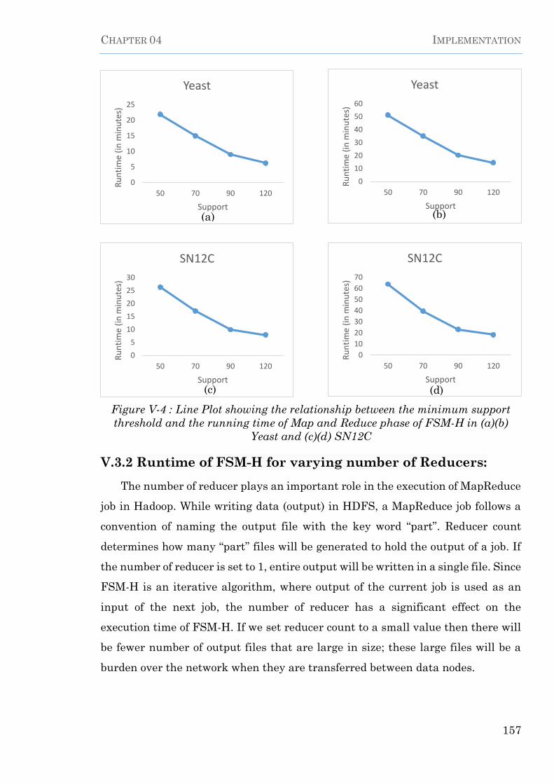
CHAPTER 04 IMPLEMENTATION
157
Figure V-4 : Line Plot showing the relationship between the minimum support
threshold and the running time of Map and Reduce phase of FSM-H in (a)(b)
Yeast and (c)(d) SN12C
V.3.2 Runtime of FSM-H for varying number of Reducers:
The number of reducer plays an important role in the execution of MapReduce
job in Hadoop. While writing data (output) in HDFS, a MapReduce job follows a
convention of naming the output file with the key word “part”. Reducer count
determines how many “part” files will be generated to hold the output of a job. If
the number of reducer is set to 1, entire output will be written in a single file. Since
FSM-H is an iterative algorithm, where output of the current job is used as an
input of the next job, the number of reducer has a significant effect on the
execution time of FSM-H. If we set reducer count to a small value then there will
be fewer number of output files that are large in size; these large files will be a
burden over the network when they are transferred between data nodes.
0
5
10
15
20
25
50 70 90 120
Ru
nti
me
(in
min
ute
s)
Support
Yeast
0
10
20
30
40
50
60
50 70 90 120
Ru
nti
me
(in
min
ute
s)
Support
Yeast
0
5
10
15
20
25
30
50 70 90 120
Ru
nti
me
(in
min
ute
s)
Support
SN12C
0
10
20
30
40
50
60
70
50 70 90 120
Ru
nti
me
(in
min
ute
s)
Support
SN12C
(a) (b)
(c) (d)

CHAPTER 04 IMPLEMENTATION
158
On the other hand, large number of reducers might create many output files
of zero size (reducer is unable to output any frequent pattern for the next stage
Mapper). These zero size output files will also become an overhead for the next
stage mappers as these files will still be used as input to a mapper. Note that,
loading an input file is costly in Hadoop.
In this experiment, we measure the runtime of FSM-H for various
configurations where we set the number of reducers to, 10, 20, 30 and 40
respectively. We run the experiment on biological datasets for a minimum support
threshold of 100 and we keep approximately 100 database graphs in each partition.
Figure V-5 (a-b) shows the relationship between execution time and the
number of reducers using bar charts. As we can see, 30 is the best choice for the
number of reducers in our cluster setup. This finding is actually intuitive, because
we have 4 data nodes each having 12 reduce slots (12 core processor), yielding 48
processing units. So keeping a few units for system use and other services, 30 is
the best choice for the number of reducers.
Figure V-5 : Bar Plot showing the relationship between the number of Reducer
and the running time of FSM-H in (a) Yeast (b) OVCAR-8..
V.3.3 Runtime of FSM-H on varying number of data nodes:
In this experiment, we demonstrate how FSM-H’s runtime varies with the
number of active data nodes (slaves). We use the Yeast dataset and 100 minimum
support threshold and keep 100 database graphs in one partition. We vary the
count of data nodes among 2, 3 and 4 and record the execution time for each of the
23.5
24
24.5
25
25.5
26
26.5
10 20 30 40
Ru
nti
me
(in
min
ute
s)
No of Reducer
Yeast
35
35.5
36
36.5
37
37.5
38
38.5
10 20 30 40
Ru
nti
me
(in
min
ute
s)
No of Reducer
OVCAR-8
(a) (b)

CHAPTER 04 IMPLEMENTATION
159
configurations. As shown in Figure V-6 (a) the runtime reduces significantly with
an increasing number of data nodes. In Figure V-6 (b) we plot the speedup that
FSM-H achieves with an increasing number of data nodes, with respect to the 2-
datanodes configuration. We can see that the speedup.
Figure V-6 : Relationship between the execution time and the number of data
nodes : (a) Bar plot shows the execution time (b) Line plot shows the speedup with
respect to the execution time using 2 data nodes configuration .
V.3.4 Effect of partition scheme on runtime:
An important requirement for achieving the optimal performance of a Hadoop
cluster is to find the appropriate number of mappers. In such a cluster, the setup
and scheduling of a task wastes a few seconds. If each of the tasks is small and the
number of tasks is large, significant amount of time is wasted for task scheduling
and setup. So the experts advise that a mapper should execute for at least 40
seconds Another rule of thumbs is that the number of mappers should not over-
run the number of partitions.
In our cluster setup, we have 4 data nodes, each with 12 cores that allow us to
have 48 mappers. Then, the perfect number of input partitions should be less than
or equal to 48. But this rules do not fit well for frequent subgraph mining task. For
example, the Yeast dataset has close to 80,000 graphs and if we make 30 partitions,
then each partition ends up consisting of 2666 graphs. Since, frequent subgraph
mining is an exponential algorithm over its input size, performing a mining task
0
10
20
30
40
50
60
70
23
4
Ru
nti
me
(in
min
ute
s)
Data nodes
Yeast
(a)
0
10
20
30
40
50
2 3 4
Spee
d-U
p (
in %
)
Support
Yeast
(b)
CHAPTER 04 IMPLEMENTATION
160
over these many graphs generally becomes computationally heavy. In this case,
the map function ends up taking more time than is expected.
As a result, the optimal number of partitions for an FSM task should set at a
much higher value (compared to a tradition data analysis task) so that the runtime
complexity of the mappers reduces significantly. Note that, the higher number of
partitions also increases the number of key-value pairs for a given pattern which
should be processed by the reducers. However, the performance gain from running
FSM over small number of graphs supersedes the performance loss due to the
increased number of key-value pairs. This is so, because the gain in execution time
in the mappers follows an exponential function, whereas the loss in execution time
in the reducers and the data transmission over the network follow a linear
function.
On the other hand, selecting the number of partitions in such a way so that,
each mapper gets to process only one transaction will not be an optimal choice.
The reason is, average processing time of only one transaction will be much less
than average task scheduling and setup time.
We will see in this experiment that increment of the number of partitions has
negative effects on overall running time.
The following experiment validates the argument that we have made in the
above paragraph. In this experiment, we run FSM-H on Yeast dataset for different
number of partitions and compare their execution time.
Figure V-7 shows the result using bar charts. The charts show that as we
increase the partition count, the performance keeps improving significantly until
it levels off at around 1000 partitions. When the partition count is 1561, there is a
slight loss in FSM-H’s performance compared to the scenario when the partition
count is 796. The strategy of finding the optimal number of partitions depends on
the characteristics of input graphs that control the complexity of the mining task,
such as the density, number of edges, number of unique labels for vertices and
edges in an input graph and so on.

CHAPTER 04 IMPLEMENTATION
161
Figure V-7 : Bar plot showing the relationship between the partition count and the
running time of FSM-H for Yeast dataset.
15
1
25
.9
26
.2
3 4 7 ( 2 0 0 ) 7 9 7 ( 1 0 0 ) 1 5 6 1 ( 1 5 0 )
Ru
nti
me(
in m
inu
tes)
No of partition(approx. # of transaction in each partition)
Yeast

Conclusion
162
VI. Conclusion:
The term “Big Data” refers to the large amounts of data in which traditional
data processing procedures and tools would not be able to handle, data is
constantly generated from various business and scientific fields, and this data data
comes in multiple forms : structured and unstructured.
Contrary to much of the traditional data types, most of the Big Data is
unstructured or semi-structured in nature, which requires different techniques
and tools to process and analyze them.
Graphs are common data structures used to represent / model real-world
systems and the data associated with it. Graph Mining is one of the arms of Data
mining in which voluminous complex data are represented in the form of graphs
and mining is done to infer knowledge from them. This thesis was focused in the
particular problem of frequent subgraph mining.
Frequent sub graph mining or for short (FSM) is extensively used for graph
classification, building indices and graph clustering purposes, the purpose of an
FSM algorithm is to discover subgraphs that appears frequently in a set of graphs
or a single large graph.
The research goals of FSM are directed at: (𝑖) effective mechanisms for
generating candidate subgraphs (without generating duplicates) and (𝑖𝑖) how best
to process the generated candidate subgraphs so as to identify the desired frequent
subgraphs in a way that is computationally efficient and procedurally effective.
The thesis presented a survey for the most FSM algorithms that are reported
in the literature, and as in the case of frequent tree mining, candidate generation
and support counting are key issues of such algorithms. Since subgraph
isomorphism detection is known to be NP-complete, a significant amount of
research work has been directed at various approaches for effective candidate
generation. The mechanism employed for candidate generation is the most
significant distinguishing feature of such algorithms.

Conclusion
163
In this thesis we studied a novel approach for frequent subgraph mining called
FSM-H, this algorithm adopt an iterative map reduce based approach for mining
graph datasets, this allows for load balancing and performance gains.
We evaluated the effectiveness of FSM-H on real graph datasets in terms of
the performance and the quality of results.
References
164
VII. References:
1. Chen M, Mao S, Zhang Y, Leung VCM. Big Data - Related Technologies,
Challenges and Future Prospects [Internet]. Springer; 2014. 89 p. Available
from: http://www.springer.com/gb/book/9783319062440
2. Rojo S. Big Data vs. Business Intelligence In Analytics | Arcadia Data
[Internet]. [cited 2018 Feb 13]. Available from:
https://www.arcadiadata.com/blog/big-data-and-business-intelligence-
differences/
3. Singh M. Effective Big Data Management and Opportunities for
Implementation [Internet]. IGI Global; 2016 [cited 2018 Feb 15]. 324 p.
Available from:
https://books.google.com/books?hl=en&lr=&id=vVOiDAAAQBAJ&oi=fnd&p
g=PR1&dq=Effective+Big+Data+Management+and+Opportunities+for+Im
plementation&ots=j__fDpC6FT&sig=uoGAzd-HZZDoEe3cA5GZJtOpxT4
4. Marr B. Why only one of the 5 Vs of big data really matters | IBM Big Data
& Analytics Hub [Internet]. [cited 2018 Feb 12]. Available from:
http://www.ibmbigdatahub.com/blog/why-only-one-5-vs-big-data-really-
matters
5. Dietrich D, Heller B, Yang B, editors. EMC Data Science and Big Data
Analytics. Wiley. Jhon Wiley & Sons, Inc.; 2015. 435 p.
6. Buyya R, Calheiros RN, Dastjerdi AV. Big Data: Principles and Paradigms.
Elsevier I. Big Data: Principles and Paradigms. Cambridge: Todd Green;
2016. 1-468 p.
7. Hurwitz J, Nugent A, Halper F, Kaufman M. Big Data for Dummies. Wiley.
Jhon Wiley & Sons, Inc.; 2013. 339 p.
8. Big Data 101 : Streaming Data - YouTube [Internet]. Wiley. [cited 2018 Jun
15]. Available from: https://www.youtube.com/watch?v=AyqRk2zrmxA
9. Tariq RS NT, RS T. Big Data Challenges. Comput Eng Inf Technol

References
165
[Internet]. 2015 Jul 29 [cited 2018 Jun 2];04(03). Available from:
http://scitechnol.com/big-data-challenges-Vfcv.php?article_id=3549
10. Big Data 101 : Big Data Technology Stack Architecture - YouTube [Internet].
[cited 2018 Feb 18]. Available from:
https://www.youtube.com/watch?v=DVMsneOBWl8
11. Azure Data Architecture Guide | Microsoft Docs [Internet]. [cited 2018 Mar
11]. Available from: https://docs.microsoft.com/en-
us/azure/architecture/data-guide/
12. Big Data 101 : Virtualization and Cloud Computing in Big Data - YouTube
[Internet]. [cited 2018 Jun 15]. Available from:
https://www.youtube.com/watch?v=kWdzc-DxYUY
13. Aridhi S. Distributed Frequent Subgraph Mining in the Cloud. Engineering
Doctoral School of Clermont Ferrand; 2013.
14. Müller DE. Lesematerial | Big Data Analytics | openHPI [Internet]. [cited
2018 May 25]. Available from:
https://open.hpi.de/courses/bigdata2017/items/4TO9c3oDe1AhP9tecEUDp5
15. Washio T, Motoda H. State of the art of graph-based data mining. ACM
SIGKDD Explor Newsl [Internet]. 2003;5(1):59. Available from:
http://portal.acm.org/citation.cfm?doid=959242.959249
16. Holder LB, Cook. Substructure Discovery in the SUBDUE System. J Chem
Inf Model. 2013;53(9):1689–99.
17. Xifeng Yan, Jiawei Han. gSpan: graph-based substructure pattern mining.
EEE Int Conf Data Min [Internet]. 2002;1(d):721–4. Available from:
http://ieeexplore.ieee.org/document/1184038/
18. Inokuchi A, Washio T, Motoda H. An Apriori-Based Algorithm for Mining
Frequent Substructures from Graph Data. 2000;13–23. Available from:
http://link.springer.com/10.1007/3-540-45372-5_2
19. Ozaki T, Ohkawa T. Mining correlated subgraphs in graph databases. In:
Pacific-Asia Conference on Knowledge Discovery and Data Mining. 2008. p.

References
166
272–83.
20. Yan X, Cheng H, Han J, Yu PS. Mining significant graph patterns by leap
search. Proc 2008 ACM SIGMOD Int Conf Manag data - SIGMOD ’08
[Internet]. 2008;433. Available from:
http://portal.acm.org/citation.cfm?doid=1376616.1376662
21. Chen C, Yan X, Zhu F, Han J. gApprox: Mining frequent approximate
patterns from a massive network. Proc - IEEE Int Conf Data Mining, ICDM.
2007;445–50.
22. Yan X, Cheng H, Han J, Xin D. Summarizing itemset patterns. Proceeding
Elev ACM SIGKDD Int Conf Knowl Discov data Min - KDD ’05 [Internet].
2005;314. Available from:
http://portal.acm.org/citation.cfm?doid=1081870.1081907
23. Huan J, Wang W, Prins J, Yang J. Spin: mining maximal frequent
subgraphs from graph databases. In: Proceedings of the tenth ACM SIGKDD
international conference on Knowledge discovery and data mining. 2004. p.
581–6.
24. Flake GW, Tarjan RE, Tsioutsiouliklis K. Graph clustering and minimum
cut trees. Internet Math. 2004;1(4):385–408.
25. Huang Y, Niu B, Gao Y, Fu L, Li W. CD-HIT Suite: a web server for
clustering and comparing biological sequences. Bioinformatics.
2010;26(5):680–2.
26. Yan X, Yu PS, Han J. Graph indexing: a frequent structure-based approach.
In: Proceedings of the 2004 ACM SIGMOD international conference on
Management of data. 2004. p. 335–46.
27. Yan X, Yu PS, Han J. Substructure similarity search in graph databases. In:
Proceedings of the 2005 ACM SIGMOD international conference on
Management of data. 2005. p. 766–77.
28. Shasha D, Wang JTL, Giugno R. Algorithmics and applications of tree and
graph searching. In: Proceedings of the twenty-first ACM SIGMOD-
SIGACT-SIGART symposium on Principles of database systems. 2002. p.

References
167
39–52.
29. Gärtner T, Flach P, Wrobel S. On graph kernels: Hardness results and
efficient alternatives. In: Learning Theory and Kernel Machines. Springer;
2003. p. 129–43.
30. Borgwardt KM, Kriegel H-P. Shortest-path kernels on graphs. In: Data
Mining, Fifth IEEE International Conference on. 2005. p. 8--pp.
31. Kashima H, Tsuda K, Inokuchi A. Marginalized kernels between labeled
graphs. In: Proceedings of the 20th international conference on machine
learning (ICML-03). 2003. p. 321–8.
32. Chakrabarti S, Dom BE, Kumar SR, Raghavan P, Rajagopalan S, Tomkins
A, et al. Mining the Web’s link structure. Computer (Long Beach Calif).
1999;32(8):60–7.
33. Kosala R, Blockeel H. Web mining research: A survey. ACM Sigkdd Explor
Newsl. 2000;2(1):1–15.
34. Getoor L, Diehl CP. Link mining: a survey. Acm Sigkdd Explor Newsl.
2005;7(2):3–12.
35. Kleinberg JM. Authoritative sources in a hyperlinked environment. In: In
Proceedings of the ACM-SIAM Symposium on Discrete Algorithms. 1998.
36. Brin S, Page L. The anatomy of a large-scale hypertextual web search
engine. Comput networks ISDN Syst. 1998;30(1–7):107–17.
37. Greco G, Guzzo A, Manco G, Sacca D. Mining and reasoning on workflows.
IEEE Trans Knowl Data Eng. 2005;17(4):519–34.
38. Hu H, Yan X, Huang Y, Han J, Zhou XJ. Mining coherent dense subgraphs
across massive biological networks for functional discovery. Bioinformatics.
2005;21(suppl_1):i213--i221.
39. Yan X. Mining, indexing and similarity search in large graph data sets. 2006;
Available from: https://www.ideals.illinois.edu/handle/2142/11256
40. Kavitha D, Rao BVM, Babu VK. A Survey on Assorted Approaches to Graph
Data Mining. Int J Comput Appl. 2011;14(1):43–6.

References
168
41. Trlnajstic N. CHEMICAL GRAPH THEORY. Randie M, Klein DJ, Mezey P
0., Trinajstic N, editors. 323 p.
42. Aldrich H, Bates T, Kuhn T. Open HPI Mooc Courses. 2001. p. 1–5.
43. Chuntao Jiang FC and MZ. A Survey of Frequent Subgraph Mining
Algorithms. Knowl Eng Rev. 2004;00(January):1–24.
44. Walks, Trails, Paths, Cycles and Circuits - Mathonline [Internet]. [cited
2018 Jun 3]. Available from: http://mathonline.wikidot.com/walks-trails-
paths-cycles-and-circuits
45. Gutman I, Polansky OE. Mathematical concepts in organic chemistry.
Springer Science & Business Media; 2012. 28 p.
46. Agrawal R, Srikant R, others. Fast algorithms for mining association rules.
In: Proc 20th int conf very large data bases, VLDB. 1994. p. 487–99.
47. Agrawal R, Srikant R. Fast Algorithms for Mining Association Rules in
Large Databases. J Comput Sci Technol [Internet]. 1994;15(6):487–99.
Available from: http://portal.acm.org/citation.cfm?id=645920.672836
48. Garey MR, Johnson DS. Computers and intractability: a guide to NP-
completeness. WH Freeman and Company, San Francisco; 1979.
49. Ullmann JR. An algorithm for subgraph isomorphism. J ACM.
1976;23(1):31–42.
50. Schmidt DC, Druffel LE. A fast backtracking algorithm to test directed
graphs for isomorphism using distance matrices. J ACM. 1976;23(3):433–45.
51. McKay BD, others. Practical graph isomorphism. 1981;45–87.
52. Cordella LP, Foggia P, Sansone C, Vento M. Subgraph transformations for
the inexact matching of attributed relational graphs. In: Graph based
representations in pattern recognition. Springer; 1998. p. 43–52.
53. Cordella L Pietro, Foggia P, Sansone C, Vento M. An improved algorithm for
matching large graphs. In: 3rd IAPR-TC15 workshop on graph-based
representations in pattern recognition. 2001. p. 149–59.

References
169
54. Pong CPTC, Shapiro LG, Haralick RM. A facet model region growing
algorithm. In: Pattern recognition and image processing Proc IEEE
Computer Society conference, Dallas, 1981,(IEEE, New York; CH1595 8).
1981.
55. Bunke H, Allermann G. Inexact graph matching for structural pattern
recognition. Pattern Recognit Lett. 1983;1(4):245–53.
56. Christmas WJ, Kittler J, Petrou M. Structural matching in computer vision
using probabilistic relaxation. IEEE Trans Pattern Anal Mach Intell.
1995;17(8):749–64.
57. Messmer BT, Bunke H. A new algorithm for error-tolerant subgraph
isomorphism detection. IEEE Trans Pattern Anal Mach Intell.
1998;20(5):493–504.
58. Conte D, Foggia P, Sansone C, Vento M. Thirty years of graph matching in
pattern recognition. Int J pattern Recognit Artif Intell. 2004;18(03):265–98.
59. Miyazaki T. The complexity of McKays canonical labeling algorithm. In:
Groups and Computation II. 1997. p. 239–56.
60. Han J, Pei J, Yin Y. Mining frequent patterns without candidate generation.
In: ACM sigmod record. 2000. p. 1–12.
61. Read RC, Corneil DG. The graph isomorphism disease. J Graph Theory.
1977;1(4):339–63.
62. Inokuchi A, Washio T, Motoda H. An apriori-based algorithm for mining
frequent substructures from graph data. In: European Conference on
Principles of Data Mining and Knowledge Discovery. 2000. p. 13–23.
63. Inokuchi A. A fast algorithm for mining frequent connected subgraphs. IBM
Res Rep. 2002;
64. Kuramochi M, Karypis G. Frequent subgraph discovery. In: Data Mining,
2001 ICDM 2001, Proceedings IEEE international conference on. 2001. p.
313–20.
65. Huan J, Wang W, Washington A, Prins J, Shah R, Tropsha A. Accurate

References
170
classification of protein structural families using coherent subgraph
analysis. In: Biocomputing 2004. World Scientific; 2003. p. 411–22.
66. Vanetik N, Gudes E, Shimony SE. Computing frequent graph patterns from
semistructured data. In: Data Mining, 2002 ICDM 2003 Proceedings 2002
IEEE International Conference on. 2002. p. 458–65.
67. Gudes E, Shimony SE, Vanetik N. Discovering frequent graph patterns
using disjoint paths. IEEE Trans Knowl Data Eng. 2006;18(11):1441–56.
68. Kuramochi M, Karypis G. Finding frequent patterns in a large sparse graph.
Data Min Knowl Discov. 2005;11(3):243–71.
69. Huan J, Wang W, Prins J. Efficient mining of frequent subgraphs in the
presence of isomorphism. In 2003. p. 549.
70. Chi Y, Wang H, Yu PS, Muntz RR. Moment: Maintaining closed frequent
itemsets over a stream sliding window. In: Data Mining, 2004 ICDM’04
Fourth IEEE International Conference on. 2004. p. 59–66.
71. Nijssen S, Kok JN. A quickstart in frequent structure mining can make a
difference. In: Proceedings of the tenth ACM SIGKDD international
conference on Knowledge discovery and data mining. 2004. p. 647–52.
72. Chaoji V, Al Hasan M, Salem S, Zaki MJ. An integrated, generic approach
to pattern mining: data mining template library. Data Min Knowl Discov.
2008;17(3):457–95.
73. Chakravarthy S, Beera R, Balachandran R. DB-Subdue: Database approach
to graph mining. In: Pacific-Asia Conference on Knowledge Discovery and
Data Mining. 2004. p. 341–50.
74. Chakravarthy S, Pradhan S. Db-fsg: An sql-based approach for frequent
subgraph mining. In: International Conference on Database and Expert
Systems Applications. 2008. p. 684–92.
75. Srichandan B, Sunderraman R. Oo-FSG: An object-oriented approach to
mine frequent subgraphs. In: Proceedings of the Ninth Australasian Data
Mining Conference-Volume 121. 2011. p. 221–8.

References
171
76. Wu B, Bai Y. An efficient distributed subgraph mining algorithm in extreme
large graphs. In: International Conference on Artificial Intelligence and
Computational Intelligence. 2010. p. 107–15.
77. Liu Y, Jiang X, Chen H, Ma J, Zhang X. Mapreduce-based pattern finding
algorithm applied in motif detection for prescription compatibility network.
In: International Workshop on Advanced Parallel Processing Technologies.
2009. p. 341–55.
78. Cook DJ, Holder LB, Galal G, Maglothin R. Approaches to parallel graph-
based knowledge discovery. J Parallel Distrib Comput. 2001;61(3):427–46.
79. Wang C, Parthasarathy S. Parallel algorithms for mining frequent
structural motifs in scientific data. In: Proceedings of the 18th annual
international conference on Supercomputing. 2004. p. 31–40.
80. Parthasarathy S, Coatney M. Efficient discovery of common substructures
in macromolecules. In: Data Mining, 2002 ICDM 2003 Proceedings 2002
IEEE International Conference on. 2002. p. 362–9.
81. Meinl T, Wörlein M, Urzova O, Fischer I, Philippsen M. The parmol package
for frequent subgraph mining. Electron Commun EASST. 2007;1.
82. Philippsen M, Worlein M, Dreweke A, Werth T. Parsemis: the parallel and
sequential mining suite. Available www2 Inform uni-erlangen
de/EN/research/ParSeMiS. 2011;
83. Wang J, Hsu W, Lee ML, Sheng C. A partition-based approach to graph
mining. In: Data Engineering, 2006 ICDE’06 Proceedings of the 22nd
International Conference on. 2006. p. 74.
84. Nguyen SN, Orlowska ME, Li X. Graph mining based on a data partitioning
approach. In: Proceedings of the nineteenth conference on Australasian
database-Volume 75. 2008. p. 31–7.
85. Bhuiyan MA, Al Hasan M. An iterative MapReduce based frequent subgraph
mining algorithm. IEEE Trans Knowl Data Eng. 2015;27(3):608–20.
86. Lakshmi K, Meyyappan T. Frequent Subgraph Mining Algorithms - a

References
172
Survey and Framework for Classification. Cs It. 2012;04:189–202.
87. Holder LB, Cook DJ, Djoko S, others. Substucture Discovery in the SUBDUE
System. In: KDD workshop. 1994. p. 169–80.
88. Kuramochi M, Karypis G. Grew-a scalable frequent subgraph discovery
algorithm. In: Data Mining, 2004 ICDM’04 Fourth IEEE International
Conference on. 2004. p. 439–42.
89. Borgelt C, Berthold MR. Mining molecular fragments: Finding relevant
substructures of molecules. In: Data Mining, 2002 ICDM 2003 Proceedings
2002 IEEE International Conference on. 2002. p. 51–8.
90. Menon R. Cloudera Administration Handbook. PACKT; 2014. 254 p.
91. Sammer E. Hadoop Operations. Vol. 53, Journal of Chemical Information
and Modeling. 2012. 283 p.
92. Big Data 101 : Storing Files in HDFS - YouTube [Internet]. [cited 2018 Jun
18]. Available from: https://www.youtube.com/watch?v=xj3_27hRPXM
93. Wu S. Big Data Processing with MapReduce. 2015;295–313.
94. Cutting D. Hadoop the Definitive Guide. White T, editor. 2009. 805 p.

Appendices
173
VIII. Appendices:
01-The application as mentioned earlier in chapter 05 works on a four node
Hadoop cluster, each machine runs CentOS v7 and Cloudera’s Distribution with
Hadoop CDH V15.4.
Each machine has a:
12 Core Intel Xeon Processor.
125 GB of RAM.
And 1.5TB of disk storage.
Yealding : 48Core for Processing, 500 GB of RAM in Total and 6TB of disk
space across the Cluster.
One of the node serves as the master as well as a slave node having the :
NameNode, and RssourceManager and DataNode Roles.
The remaining Three have each :
DataNode and the NodeManager Roles.
The following lists the /etc/hosts file on each of the machines:
10.42.0.2 master.FSMCluster.local master
10.42.0.3 datanode1.FSMCluster.local datanode1
10.42.0.4 datanode2.FSMCluster.local datanode2
10.42.0.5 datanode3.FSMCluster.local datanode3
02-We used for the purpose of running the application: 32 Cores and a total of
320 GB of RAM across the Cluster, and a 6TB of disk space for the purpose of DFS
Storage, the remaining resources are reserved to the system overhead.
Here are some configuration parameters (organized in groups) that were
necessary for getting the best performance according to our setup :

Appendices
174
A- YARN Container Configuration Property (Vcores) : Configuration parameter Value yarn.scheduler.minimum-allocation-vcores 1 yarn-scheduler.maximum-allocation-vcores 1 yarn.scheduler.increment-allocation-vcores 1
B- YARN Container Configuration Property (Memory):
Configuration parameter Value yarn.scheduler.minimum-allocation-mb 1024 yarn.scheduler.maximum-allocation-mb 10240 yarn.scheduler.increment-allocation-mb 512
C- MapReduce Configuration:
Configuration parameter Value yarn.app.mapreduce.am.resource.cpu-vcores 1 yarn.app.mapreduce.am.resource.mb 10240 ApplicationMaster Java Maximum Heap Size (available in CM) 10240 mapreduce.map.cpu.vcores 1 mapreduce.map.memory.mb 10240 mapreduce.map.java.opts.max.heap 10240 mapreduce.reduce.cpu.vcores 1 mapreduce.reduce.memory.mb 10240 mapreduce.reduce.java.opts 10240 mapreduce.task.io.sort.mb 256