TREBALL FI DE MÀSTER

Màster en Enginyeria Química esp. Polimers

INJECTION MOLDING OPTIMIZATION IN ORDER TO IMPROVE

THE DISPERSION OF THE NANOCLAYS

Memòria i Annexos

Autor: Enric Pascual Cuenca

Director: Alfonso Rodríguez Galán

Co-Director: Encarnación Escudero Martínez

Convocatòria: Maig 2018

Memoria

1

Memoria

2

Abstract

Injection molding is the most commonly manufacturing process used for the fabrication of plastic parts.

Different products can be manufactured using injection molding which vary greatly in their size,

complexity and application. Automotive industry is the most important sector that uses this technology.

A wide variety of additives are used to modify the raw polymers and achieve new properties.

Nanoadditives and nanoclays specifically, are used to improve various physical properties, such as

reinforcement, synergistic flame retardant and barrier.

This work is focused on the study the different parameters in the injection molding process in order to

optimize the process using a specific grade of polypropylene and a specific grade of nanoclay. The main

goal of the project is to improve the flexural modulus of the studied part using a lineal model taking into

account the behavior the selected parameters.

Memoria

3

Memoria

4

Index

1. Introduction .......................................................................................................................................... 6

1.1. Polymer processing ....................................................................................................................... 7

1.2. Injection molding process ............................................................................................................. 9

1.3. Thermoplastic nanocomposites .................................................................................................. 11

1.4. Nano-clays ................................................................................................................................... 14

2. State of the art: Automotive Sector .................................................................................................... 16

3. Objective ............................................................................................................................................. 19

4. Experimental ....................................................................................................................................... 20

4.1. Materials ..................................................................................................................................... 20

4.2. Injection molding machine ......................................................................................................... 22

4.3. Injection molding tool ................................................................................................................. 24

4.4. Characterization methods ........................................................................................................... 25

4.5. Injection molding process optimization ...................................................................................... 28

4.6. Design of experiments (DOE) ...................................................................................................... 38

4.7. Lineal modelling .......................................................................................................................... 40

4.8. Residuals ..................................................................................................................................... 41

4.9. Model signification study ............................................................................................................ 44

4.10. Model validation ..................................................................................................................... 46

4.11. Results ..................................................................................................................................... 48

5. Conclusions ......................................................................................................................................... 50

6. References .......................................................................................................................................... 52

7. Annex .................................................................................................................................................. 56

7.1. Annex 1. Surface responses ........................................................................................................ 56

Memoria

5

Memoria

6

1. Introduction

Injection molding process is one of the most important technology used in the automotive industry. Three

main components are required: injection molding machine (IMM), tool or mold and plastic pellets.

Depends on the final part, different plastic will be selected based on the final part properties.

Additives are usually used with the aim of enhance some properties of the standard material.

Nanoadditives are commonly used to enhance properties like barrier properties, mechanical properties,

thermal properties, optical properties among others. Good dispersions is related directly to a high

performance of these nanofiller within the polymer matrix.

All experiment carried out during this work were performed in EURECAT, a technology center in Catalonia.

EURECAT-Cerdanyola has experience in plastic injection for more than 30 years. The center participates

in public and private projects researching in different applications using the injection molding process as

a basis.

This work is focused on study how some injection parameters may affect to the dispersion of the

nanoadditives and the mechanical properties of the final part.

Memoria

7

1.1. Polymer processing

There are many different types of plastics processed by different methods to produce products meeting

many different performance requirements, including costs. The basics in processing relate to

temperature, time and pressure. In turn they interrelate with product requirements, including plastics

type and the process to be used. Europe plastics consumtion in 2016 was 60 million tonnes and the

worldwide plastic consumtion was 355 million tones. Packaging is the market sector which converts 39.9%

of the consumtion and the autmotive sector consumes 10% of the total in Europe.

All of this processes are used to fabricate all types and shapes of plastic products; household convenience

packages, electronic devices and many others, including the strongest products in the world, used in space

vehicles, aircraft, building structures, and so on.

Proper process selection depends upon the nature and requirements of the plastic, the properties desired

in the final product, the cost of the process, its speed, and product volume. Some materials can be used

with many kinds of processes; others require a specific or specialized machine. Numerous fabrication

process variables play an important role and can markedly influence a product's esthetics, performance,

and cost. The relative use of these methods in Europe in 2016 is shown in Fig. 1 [1].

Figure 1. Plastic consumption by process. Europe 2016

Many of these variables and their behaviors are the same in the different processes, as they all relate to

temperature, time, and pressure. The process depends on several interrelated factors: (1) designing a part

to meet performance and manufacturing requirements at the lowest cost; (2) specifying the plastic; (3)

specifying the manufacturing process, which requires (a) designing a tool 'around' the part, (b) putting the

'proper performance' fabricating process around the tool, (c) setting up necessary auxiliary equipment to

interface with the main processing machine, and (d) setting up 'completely integrated' controls to meet

the goal of zero defects; and (4) 'properly' purchasing equipment and materials, and warehousing the

materials.

Major advantages of using plastics include formability, consolidation of parts, and providing a low cost-

to-performance ratio. For the majority of applications that require only minimum mechanical

Extrusion36%

Injection32%

Blow10%

Calendring6%

Coating5%

Compression3%

Powder2%

Others6%

Memoria

8

performance, the product shape can help to overcome the limitations of commodity resins such as low

stiffness; here improved performance is easily incorporated in a process. However, where extremely high

performance is required, reinforced plastics or composites are used.

Polymers are usually obtained in the form of granules, powder, pellets, and liquids. Processing mostly

involves their physical change (thermoplastics), though chemical reactions sometimes occur (thermosets).

Two of the main characteristics of the processing methods are compared in Fig. 2 [1]. One group consists

of the extrusion processes (pipe, sheet, profiles, etc.). A second group takes extrusion and sometimes

injection molding through an additional processing stage (blow molding, blown film, quenched film, etc.).

A third group consists of injection and compression molding (different shapes and sizes), and a fourth

group includes various other processes (thermoforming, calendaring, rotational molding, etc.).

Figure 2. Process characteristics graph

The common features of these groups are (1) mixing, melting, and plasticizing; (2) melt transporting and

shaping; (3) drawing and blowing; and (4) finishing. Mixing, melting and plasticizing produce a plasticized

melt, usually made in a screw (extruder or injection). Melt transport and shaping apply pressure to the

hot melt to move it through a die or into a mold. The drawing and blowing technique stretches the melt

to produce orientation of the different shapes (blow molding, forming, etc.). Finishing usually means

solidification of the melt. The most common feature of all processes is deformation of the melt with its

flow, which depends on its rheology. Another feature is heat exchange, which involves the study of

thermodynamics. Changes in a plastic's molecular structure are chemical.

0

1

2

3

4

5Blow molding

Injection Molding

CompressionThermoforming

Extrusion

Part complexity Part size

Memoria

9

1.2. Injection molding process

Injection molding is a repetitive process in which melted (plasticized) plastic is injected into a mold cavity

or cavities, where it is held under pressure until it is removed in a solid state, basically duplicating the

cavity of the mold. The mold may consist of a single cavity or a number of similar or dissimilar cavities,

each connected to flow channels, or runners, which direct the flow of the melt to the individual cavities.

The process is divided in three steps: (1) heating the plastic in the injection or plasticizing unit so that it

will flow under pressure, (2) allowing the plastic melt to solidify in the mold, and (3) opening the mold to

eject the molded product. These three steps are the operations in which the mechanical and thermal

inputs of the injection equipment must be coordinated with the fundamental properties and behavior of

the plastic being processed; different plastics tend to have different melting characteristics, with some

being extremely different. They are also the prime determinants of the productivity of the process, since

the cycle time (Fig. 3) will depend on how fast the material can be heated, injected, solidified, and ejected.

Depending on shot size and/or wall thicknesses, cycle times range from fractions of a second to many

minutes. Other important operations in the injection process include feeding the injection molding

machine (IMM), usually gravimetrically through a hopper, and controlling the barrel’s thermal profile to

ensure high product quality.

Figure 3. Typical cycle time break-down

IMMs are characterized by their shot capacity and their clamping force. A shot represents the maximum

volume of melt that is injected into the mold. It is usually about 20 to 80% of the actual available volume

in the barrel. Injection pressure in the barrel can range from 15 to 400 MPa. The characteristics of the

plastic being processed determine what pressure is required in the mold to obtain good products. Given

Memoria

10

a required cavity pressure, the barrel pressure has to be high enough to meet pressure flow restrictions

going from the barrel into the mold cavity or cavities.

Otherwise, the clamping force on the mold halves required in the IMM also depends on the plastic being

processed. A specified clamping force is required to retain the pressure in the mold cavity. It also depends

on the projected area of any melt located on the parting line of the mold, including any cavities and mold

runner(s) that are located on the parting line. By multiplying the pressure required to inject the part and

the projected area, the clamping force required is determined. To provide a safety factor, 10 to 20%

should be added.

Many thousands of different plastics (also called polymers, resins, reinforced plastics, elastomers, etc.)

are processed every year. Each of the plastics has different melt behavior, product and cost. To ensure

that the quality of the different plastics meets requirements, tests are carried out on melts as well as

molded products. There are many different tests to provide all kinds of information. Important tests on

molded products are mechanical tests.

There are basically two types of plastic materials molded: 1) thermoplastics (TPs), which are

predominantly used, can go through repeated cycles of heating/melting usually at least to 260°C and

cooling/solidification. The different TPs have different practical limitations on the number of heating-

cooling cycles before appearance and/or properties are affected. Thermosets (TSs), upon their final

heating [usually at least to 120°C, become permanently insoluble and infusible. During heating they

undergo a cross-linking process. Certain plastics require higher melt temperature, some may require

400°C. Most of the literature on injection molding processing refers entirely or primarily to TPs; very little,

if any at all, refers to thermoset TS plastics. At least 90% of all injection-molded plastics are TPs.

Memoria

11

1.3. Thermoplastic nanocomposites

Extensive compounding of different amounts and combinations of additives (colorants, flame retardants, heat and light stabilizers, etc.), fillers (calcium carbonate, etc.), and reinforcements (glass fibers, glass flakes, graphite fibers, whiskers, etc.) are used with plastics.

Thermoplastic nanocomposites are the combinations between a nanostructured inorganic or organic filler with size typically between 1 and 100 nm in at least one dimension, and a polymeric matrix. The main advantage of use this fillers over the conventional composite material is the extremely high surface area, which have proportionally more surface atoms than their micro-scale counterparts, thus allowing intimate interphase interactions and conferring extraordinary properties to the polymer. The size of the nano-fillers favors the use of small amount of them and a more effective transfer to the polymer matrix of their unique molecular properties.

Typical nano-fillers include nanoclays, carbon nanotubes (CNT), nanoparticle silver, nanoalumina, among others. Nanocomposite materials exhibit unique material properties, such as improved barrier properties, flame retardant, and mechanical properties, depending on the choice of filler. This materials have application for lighter weight structural parts, barrier materials for improved packaging (e.g MREs), EMI shielding, and antimicrobial performance.

Compound processing of polymers is mainly performed via extrusion. Extrusion allows melting a polymer with a high energy input during short time. Due to the supply of heat and energy input caused by friction between the screws, the mass melts, becomes formable and is pressed through the extruder die [2]. During the whole process the mass can be compressed, mixed, plasticized, homogenized, chemically transformed, degasificated or gasificated [3], [4]. It is also possible to incorporate nanoparticles in a compounding process, in the last years different types of nano-composites are available. In case of processing exfoliated nano-composites, the dispersion quality mainly depends on the extruder and screw configuration [5]. Exfoliation is favored at high shear rates [6], while longer residence time favors a better dispersion [5]. Also, the location where the nano-clay is introduced has been shown to be an important factor [7]. However, the major factor whether a good dispersion or exfoliation is possible is the thermodynamic affinity between the nanoclay/nanoparticle and the polymer matrix [8]. When attractive interactions between matrix and nanoclay are not sufficient, intercalation is acquired, while exfoliation can be obtained when strong attractive interactions are present [9]. Figure 4 shows how exfoliation can be achieved via extrusion/melt processing [8].

The nanocomposite performance depends on number of nanoparticles features such as the size, aspect ratio, specific surface area, volume fraction used, compatibility with the matrix and dispersion. In fact, although a long time has gone in the nanocomposites’ era, the dispersion state of nanoparticles remains the key challenge in order to obtain the full potential of properties enhancement at lower filler loading than for microcomposites. Not only the nanoparticles themselves can explain the observed effects, the impact of the interface between the matrix and particle also play a very important role. Indeed, the extremely high surface area leads to change in the macromolecular state around the nanoparticles (e.g. composition gradient, crystallinity, changed mobility, etc.) that modifies the overall material behavior [10].

Memoria

12

Figure 4. Mechanism of organoclay dispersion and exfoliation during melt processing [50, 52]

The nanoparticles dispersion can be characterized by different states at nano-, micro- and macroscopic scales. For example, nanoclay based composites can show three different types of morphology: immiscible (eg. microscale dispersion, tactoid), intercalated or exfoliated (miscible) composites [8]. The affinity between matrix and filler increases from tactoid over intercalated to exfoliated clays [6].

Different techniques can be used to study the dispersion quality of nano-particles within the polymeric matrix: XRD, SEM, TEM, infrared spectroscopy (IR) and atomic force microscopy (AFM). Figure 5 shows the different states of dispersion for a nano-composite prepared with nano-clays and a polymer matrix, using TEM and XRD and its correspondent illustration.

Widely performed melt processes specialized in packaging and automotive are injection molding, film extrusion and extrusion coating. Since many different process parameters have a direct influence on the processed materials, Taguchi methods are commonly used in plastic injection molding industry as a robust optimization technique for applications from product design to mold design; and from optimal material selection to processing parameter optimization. Pötschke et al. (2008) studied the influence of injection molding parameters on the electrical resistivity of nanocomposite formed by PP/CNT using a four-factor factorial design with keeping pressure, injection velocity, mold temperature and melt temperature. Sample with lower melt temperature and higher injection velocity shown a better dispersion compared with injection molded at low velocity and high melt temperature [11]. Chandra et al. (2007) summarized their research on PC and CNT nanocomposite in order to achieve homogeneous distribution of CNT and to obtain high electrical conductivity the nanocomposites should be processed at high melt temperatures and low injection speeds to ensure proper and uniform electrical conductivity [12]. Recently, the F. Stan group has made a study about the influence of the process parameters in the nanocomposite (PP/CNT) to improve the mechanical properties. The injection molding parameters affect the degree of crystalline morphology of the molded polymers. Therefore, these effects could affect the physical and mechanical properties of the injection molded parts. On the other hand, the effect of crystallinity on the mechanical properties is less important than the effect of the carbon nanotubes. Their research work, concluded that the most significant injection molding parameter is the injection pressure [13].

Memoria

13

Figure 5. Different states of nano-additive’s dispersion. a)TEM, b) XRD.

Additionally, the use of compatibilizers can change the optimal parameters to the process. P. Constantino et al. studied the microstructure of the same nanocomposites PP/nanoclay produced by a non-conventional method of extrusion, SCORIM (Shear Controlled Orientation in Injection Molding). This method is based on the concept of in-mold shear manipulation of the melt during the polymer solidification phase. The degree of clay exfoliation not only depends on the affinity and compatibility of the organoclay with the matrix, but also on the shear stress which is an extrinsic factor dependent on processing conditions and clay loading. High shear rate induced a thicker skin, while high temperature induced a thinner skin [14]. An interesting work was made by P.F. Rios, comparing the behavior of different polymers with the same nanofiller. He studies the influence of injection molding parameters in HDPE, PA6, PA66, PBT and PC with carbon nanotubes. The main objective was to evaluate the electrical resistivity, thermal conductivity and the mechanical properties. The literature reveal how the different parameters of the injection molding process might affect directly in the quality of the part injected and their properties. The formulation is important, but the process parameters show a relevant importance [15].

Memoria

14

1.4. Nano-clays

From the end of the last century, the discovery of various clays and their use in a variety of applications

resulted in a continuous developments in polymer science and nanotechnology. The term ‘clay’ is referred

to a class of materials generally made up of layered silicates or clay minerals with traces of metal oxides

and organic matter. Clay minerals, usually crystalline, are hydrous aluminum phyllosilicates, sometimes

with variable amounts of iron, magnesium, alkali metals, alkaline earths, and other cations.

As a low cost inorganic material, clays are used in industrial, engineering and scientific fields. In science,

these are commonly also used as catalysts, decoloration agents and adsorbents and in industrial and

engineering fields, these are used in oil drilling, ceramics and the paper industry.

Generally, clay particles have lateral dimensions of centimeters, micrometers in one dimension and the

thickness of a single clay platelets in order of nanometers. These layered clays are characterized by strong

intralayer covalent bonds within the individual sheets comprising the clay [16]. This is the reason why

dispersion of them in a polymer matrix is very difficult during the preparation of polymer nano-

composites, generally requiring modification of the clay.

Figure 6. Classification of natural clay

The modification of the space between layers of clay by intercalating long chains or by grafting with

different functional groups results in a change from hydrophilic to hydrophobic character, and a wide

range of new and fascinating properties. Therefore, nowadays the modification of clay has a lot of interest

in the preparation of polymer-clay nanocomposites [17], [18]. However, the nanolayers of the clay tend

to stack face to face leading to agglomerated tactoids in nanocomposites, which may work again the

properties of the individual components. The dispersion of the tactoids into discrete monolayers is related

to the intrinsic incompatibility of hydrophilic clay and hydrophobic engineering polymers. Since proper

dispersion of these nanostructures in a polymer matrix is essential for the improvement of material

properties compared with pristine polymer or conventional micro- and macro-composites [19], [20].

Memoria

15

Different methods have been developed in order to improve the clays dispersion, based on two main

methods of modification: (1) physical absorption and (2) chemical modifications, such as grafting

functional polymers or functional groups on to the surface of clay or ion exchange with organic cations or

anions [17]. First method is based on thermodynamics which improves their physical and chemical

properties for composite and the structure of the clays remain unaltered. In this case, exists a weak force

between the adsorbed molecules and the clay is an important disadvantage. Otherwise, the second

method improves the interaction force between clays and modifiers, controlling and tuning their

properties.

Generally, clay can be classified into two categories: natural and synthetic clays. Figure 6 shows the

classification of natural clays. They are basically composed of alternating sheets of SiO2 and AlO6 units in

ratios of 1:1 (kaolinite), 2:1 (montmorillonite and vermiculite) and 2:2 (chlorite) [21]. Modification of clay

minerals such as organoclay and organo-modified clay is a new path of clay mineral research.

Memoria

16

2. State of the art: Automotive Sector

The basic trends that nanotechnology enables for the automobile are

lighter but stronger materials (for better fuel consumption and increased safety)

improved engine efficiency and fuel consumption for gasoline-powered cars (catalysts; fuel

additives; lubricants)

reduced environmental impact from hydrogen and fuel cell-powered cars

improved and miniaturized electronic systems

better economies (longer service life; lower component failure rate; smart materials for self-

repair)

The use of polymer nanocomposites in the manufacturing chain started in 1991 when Toyota Motor Co.,

in collaboration with Ube Industries, introduced nylon-6/clay nano composites in the market to produce

timing belt covers as a part of the engine for their Toyota Camry cars [22]. Then, Japan introduced nylon-

6 nanocomposites for engine covers on Mitsubishi GDI engines [23] manufactured by injection moulding.

The product is said to offer a 20% weight reduction and excellent surface finish. In 2002, General Motors

launched a step-assist automotive component made of polyolefin reinforced with 3% nanoclays, in

collaboration with Basell (now LyondellBasell Industries) for GM's Safari and Chevrolet Astro vans,

followed by the application of these nanocomposites in the doors of Chevrolet Impalas [24], [25].

The important increase in the commercialization of nanocomposites production occurred over the last

years. In 2009, a one-piece compression moulded rear floor assembly was manufactured by General

Motor for their Pontiac Solace using nano-enhanced Sheet Moulding Compounds (SMCs) developed by

Molded Fiber Glass Companies (MFG), Ohio. This technology is also in use on GM's Chevrolet Corvette

Coupe and Corvette ZO6. The nano-filled SMCs exhibit significantly lower density than conventional SMCs

resulting in improved fuel efficiency [26]. At this point, the automotive industry can benefit from this

material in several applications such engines, suspension, break systems, frames and body parts, paints

and coatings, tires and electric and electronic equipment.

In the latter part of the 1980s and the beginning of the 1990s, a research team from Toyota Central

Research Development Laboratories (TCRDL) in Japan reported a work on a Nylon-6/clay nanocomposite

and disclosed improved methods for producing nylon-6/ clay nanocomposites using in situ polymerization

similar to the Unichika process [27] [28] [29] [30].

he research findings demonstrated a significant improvement in a wide range of physico-mechanical

properties by reinforcing polymers with clay on the nanometer scale [31] [32]. The Toyota research team

also reported various other types of clay nanocomposites based on polymers such as polystyrene, acrylic,

polyimides, epoxy resin, and elastomers using a similar approach [33] [34] [35] [36] [37]. Since then,

extensive research in nanocomposites field has been carried out worldwide. Figure 7 shows timeline for

the commercialization of products by automotive players.

Memoria

17

Figure 7. Timeline for the commercialization of products by automotive players.

Among nanomaterials, nanoclays are the most commonly used commercial additive for the preparation

of nanocomposites, accounting for nearly 80% of the volume used. Carbon nanofibers, carbon nanotubes

(mainly MWCNTs), and Polyhedral Oligomeric Silsesquioxanes (POSS) are also being used commercially in

nanocomposites, gaining ground fast with improvements in cost/performance and processability

characteristics.

The OEMs/Tier I, Tier II, Tier III, raw materials/nanointermediates manufacturers, researchers and

technologists are realizing that other than clays, nanomaterials like graphene, carbon nanofibers,

nanofoams, multiscale hybrid reinforcement and graphene-enabled rubber nanocomposites could drive

the market dynamics.

The price and performance advantages of graphene are challenging carbon nanotubes in polymer

nanocomposites applications due to its intrinsic properties and it is predicted that a single, defect-free

graphene platelet could have an intrinsic tensile strength higher than that of any other material [38].

In June 2010, a U.S. Patent was granted to The Trustees of Princeton University for functional graphene-

rubber nanocomposites [39], which can be produced at a much lower cost than carbon nanotubes and

exhibits excellent mechanical strength, superior toughness, higher thermal stability and electrical

conductivity. This graphene-rubber nanocomposite can be employed in all the areas for gas barrier

applications including tires and packaging.

Memoria

18

Another patent was granted in 2011, for a composite material of nanoscale graphene and an elastomer

for vehicle tire application [40]. The multiscale hybrid reinforcement is another potential polymer

nanocomposite material for the automotive industry due to its enhanced load transfer at the

reinforcement/matrix interface, i.e. by tailoring the interfacial shear strength, which is made of micro

sized carbon-fibre yarns and fabrics coated with carbon nanostructures. The high performance racing cars

and high-end sports cars require excellent properties such as structural stiffness, heat shielding, impact

and compressive strength, and many others.

Otherwise, different works has been carried out regarding to the surface properties of the produced parts

in order to enhance their properties. In 2009, viscoelastic properties and scratch morphologies were

studied using various amounts of nano silica [41]. Different nano-silica particles were incorporated in an

automotive OEM clear-coat based on acrylic/melamine chemistry in order to study their effect in the

scratch/mar resistances using nano-indentation hardness measurements [42]. In 2014, H. Yari, et. al.

studied the influence of OH-functionalized polyhedral oligomeric silsesquioxane(POSS) nano-structure in

the same clear coat [43].

In 2015, the impact behaviour of hybrid nano-/micro-modified composite was investigated in Glass Fiber

Reinforced Plastics (GFRP). The hybrid nano-/micro fillers chosen were Cloisite® 30B nanoclay and 3M™

Glass Bubbles iM16K [44].

Memoria

19

3. Objective

The aim of this project is to optimize the injection molding process to achieve the best nano-additive

dispersion in order to improve mechanical properties of the injected part.

A good dispersion of the nano particles and their compatibility with the matrix polymer are the two critical

points to assure the improvement of the properties comparing with the raw polymer. This work will be

focused on the dispersion of the nano additives during the injection molding. A study of the interaction

between some injection parameters and the dispersion will be carry out.

First of all, the injection molding process needs to be optimized taking into account the most relevant

injection parameters during the process, using Scientific Injection Molding (SIM). Once the process is

optimized for the selected thermoplastic composite, injection tool and injection molding machine, four

injection parameters will be selected to study their behavior related to the dispersion of the nanofiller.

A mathematical model will be used to study how each parameter affect to the dispersion of the composite

and determine which parameter combination enhance the selected mechanical property.

In this work, Flexural Modulus is selected as an output of the linear model. Considering the Flexural

Modulus of the raw polypropylene, the goal of the project will be to increase this value as much as

possible.

Memoria

20

4. Experimental

In order to characterize the material within the project, a dog-bone specimens were produced using a

special mold. Standardized specimens were tested and this data was used as an input to carry out a

mathematical model.

First step was to select the most important injection parameters related to the nano-additive dispersion

and then to set up a design of experiments to study their behavior related to the dispersion.

4.1. Materials

Plastic used to carry out this work is made up of two commercial grades: polypropylene and nanoclay

additive. The formulation is composed by 8 wt. % of nanoclay.

4.1.1. Polymer matrix

Polymer used during the whole work was polypropylene, in particular ISPLEN PP080G2M from Repsol.

This is a homopolymer grade characterised by good flow properties that enables to fill the mould easier

and by short cycle times with big articles. Parts manufactured with this grade have excellent chemical

resistance, are easily decorated and can accept different colouring systems.

Recommended melt temperatures range from 190 to 250°C. Main properties are shown in Table 1:

PROPERTIES VALUE UNIT METHOD General Melt flow rate (230°C/ 2,16 kg) 20 g/10 min ISO 1133 Density at 23ºC 905 kg/m3 ISO 1183 Mechanical Flexural modulus of elasticity 1600 MPa ISO 178 Charpy impact strength (23°C,notched) 3 kJ/m2 ISO 179 Thermal HDT 0,45 MPa 85 °C ISO 75 Others Shore Hardness 70 - ISO 868

Table 1. Matrix polymer properties

This material should be stored in a dry atmosphere, on a paved, drained and not flooded area, at

temperatures under 60ºC and protected from UV radiation. Regarding to the pre-treatment of the

material, it is not necessary to pre-dry the material due it not contains mineral additives.

Memoria

21

4.1.2. Nanoclay additive

The nanoclay used during this work was Cloisite 20 from BYK. This grade is bis(hydrogenated tallow

alkyl)dimethyl, salt with bentonite. In Table 2 are shown the typical properties of this grade:

PROPERTIES VALUE UNIT Moisture <3 % Typical Dry Particle Size <10 μm (d50) Color Off White Packed Bulk Density 175 g/l Density 1.77 g/cm3

X Ray Results 3.16 nm (d001) Table 2. Nanoclay main properties

Using this material as an additive with the matrix, a pre-drying was needed in order to avoid processability

problems during the injection process.

Memoria

22

4.2. Injection molding machine

An ENGEL E-motion 200/55 full electric was used in Eurecat to inject the dog-bone specimens and

therefore to test the mechanical properties of the samples. Technical specifications of the machine used

are shown in Table 3 and a picture of the machine in the Figure 8.

VALUE UNIT

Clamping unit

Clamping force 550 kN

Opening stroke 270 mm

Ejector stroke 100 mm

Ejector force 23 kN

Injection unit

Screw diameter 25 mm

Max swept volume 59 cm3

Screw speed max 400 r/min

Screw speed max current 400 r/min

Injection rate 109 cm3/s

Injection rate increased 109 cm3/s

Spec. Injection pressure 2400 bar

Spec. Injection pressure increased 2400 bar

Nozzle stroke 225 mm

Nozzle cont. pressure 28 kN Table 3. Injection machine specifications

The election of this machine was determined by the mould used to inject the samples. There are some

advantages of using fully electric injection moulding machines:

Electric machines are digitally controlled and mechanically driven. Their processes do not vary

over time since they have no hoses to expand, no valves to potentially stick and no hydraulic fluid

to heat up or compress.

Electric machines turn injection moulding into a more predictable operation. With a more

consistent machine, the same process setup can be used repeatedly, without affecting part

consistency or quality. For example, screw position for fill and pack is controlled with digital

precision, eliminating over-packing and greatly reducing moulded-in stress. Consistent machine

performance also allows labour cost reductions with unmanned shifts at night or on weekends.

Utilization of skilled labour is greatly enhanced.

From the day the machine starts up, it reduces cost per part. All-electric machines produce faster

cycle times because of independent clamp/injection functions. Their precision shot control saves

material and prevents using more resin, colorant or additive than the part needs.

Memoria

23

Figure 8. IMM used for this work

Memoria

24

4.3. Injection molding tool

A mould was manufactured in order to obtain samples to carry out mechanical characterization. Four

different standardized specimens can be injected as shown in Figure 9:

A. Tensile strength B. Hardness C. Tensile strength for thermoplastic elastomers D. Impact

Figure 9. Standardized specimens which can be manufactured with injection

The mould was designed with selectors to choose what part/s could be injected. Figure 10 shows the

ejection side with the four parts and the sprue selector and the injection side. Injection side was equipped

with a hot runner in order to ease the injection and to reduce the waste of material.

Figure 10. Ejection side (left) and injection side (right).

Only the A specimen were injected within the frame of the project. A variety of specimen shape can be

used for this test, but the most commonly used specimen size for ASTM is 3.2mm x 12.7mm x 125mm and

for ISO is 10mm x 4mm x 80mm. Figure 11 shows the dimensions of the standard sample used:

Figure 11. Left: Standard sample dimensions. Right: 3D model of the sample

Memoria

25

4.4. Characterization methods

Different methods were used to characterize the material used within the work. Regarding to the

mechanical properties, a Flexural Modulus test was carried out. On the other hand, two rheology

properties were measured. Rheology properties are important when processing the material. Using

additives may cause variations in some properties that can cause problems during the injection molding

process.

Following are shown the methods used, equipment used and test conditions:

4.4.1. Density

Density is the mass per unit volume of a material. Specific gravity is a measure of the ratio of mass of a

given volume of material at 23°C to the same volume of deionized water. Specific gravity and density are

especially relevant because plastic is sold on a cost per kilogram basis and a lower density or specific

gravity means more material per kilogram or varied part weight.

Equipment: Electronic Densimeter METROTEC MD300S

Test conditions:

Standard: UNE EN ISO 1183-1 (2004)

A method: Immersion method for solid plastics (except dust).

Sample preparation: standardized test section 4 x 10 mm

Immersion liquid: Distilled water

Test atmosphere:

Test temperature: 20 ± 1⁰C

4.4.2. Flow rate determination (MFR)

Melt Flow Rate measures the rate of extrusion of thermoplastics through an orifice at a prescribed

temperature and load. It provides a means of measuring flow of a melted material which can be used to

differentiate grades as with polyethylene, or determine the extent of degradation of the plastic as a result

of molding. Degraded materials would generally flow more as a result of reduced molecular weight, and

could exhibit reduced physical properties. Typically, flow rates for a part and the resin it is molded from

are determined, then a percentage difference can be calculated. Alternatively, comparisons between

"good" parts and "bad" parts may be of value.

Approximately 7 grams of the material is loaded into the barrel of the melt flow apparatus, which has

been heated to a temperature specified for the material. A weight specified for the material is applied to

a plunger and the molten material is forced through the die. A timed extrudate is collected and weighed.

Melt flow rate values are calculated in g/10 min. At least 14 grams of material is needed.

Equipment: CEAST Modular Flow Index

Memoria

26

Test conditions:

Standard: EN ISO 1133-1 (2011)

Method: procedure B of the standard

Amount of material in the cylinder: 7 g

Test temperature: 230ºC (for PP) and 190ºC (for PE and PHB)

Weight: 2.16 Kg

Filter size: 8 mm

Filter diameter: 2,095mm

Number of readings: minimum 40

Drying of the sample prior minimum 2 h at 90 ° C in convection oven

4.4.3. Flexural strength test

The flexural test measures the force required to bend a beam under three point loading conditions. The

data is often used to select materials for parts that will support loads without flexing. Flexural modulus is

used as an indication of a material’s stiffness when flexed. Since the physical properties of many materials

(especially thermoplastics) can vary depending on ambient temperature, it is sometimes appropriate to

test materials at temperatures that simulate the intended end use environment.

Most commonly the specimen lies on a support span and the load is applied to the center by the loading

nose producing three point bending at a specified rate. The parameters for this test are the support span,

the speed of the loading, and the maximum deflection for the test. These parameters are based on the

test specimen thickness and are defined differently by ASTM and ISO. For ASTM D790, the test is stopped

when the specimen reaches 5% deflection or the specimen breaks before 5%. For ISO 178, the test is

stopped when the specimen breaks. Of the specimen does not break, the test is continued as far a possible

and the stress at 3.5% (conventional deflection) is reported.

Equipment: Universal Testing Machine INSTRON 6025

Test conditions:

Standard: UNE EN ISO 178 (2013)

Cell load: 50 KN

Type test: standard Section 4 x 10 mm

Distance between supports 64 mm

Calculation of modulus of elasticity:

- Preload: 2N 1 mm / min

- Measuring Range: 0:05 to 12:25%

- Speed: 2mm / min

Speed trial: 10mm / min

deformation maximum 10%

Num. specimens 5

Test atmosphere:

Memoria

27

Temperature: 23 ± 2 ° C

Relative Humidity: 50 ± 10%

4.4.4. Material properties comparison

In order to ensure the good processability of the composite injected in this work, a comparison

between raw polymer and the nano composite was carried out using the methods described above:

Material MFI (2,16kg 230ºC) MFI (2,16kg 230ºC) Density theory

Density measured

cc/10'' g/10'' g/cm3 g/cm3 Raw PP 25,0 22,6 0,905 0,906 NCC - - 1,770 - Compound 28,5 26,3 0,928 0,920

Table 4. Comparison between raw polymer and the nanocomposite

Memoria

28

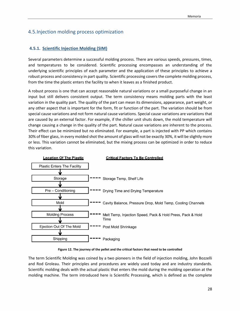
4.5. Injection molding process optimization

4.5.1. Scientific Injection Molding (SIM)

Several parameters determine a successful molding process. There are various speeds, pressures, times,

and temperatures to be considered. Scientific processing encompasses an understanding of the

underlying scientific principles of each parameter and the application of these principles to achieve a

robust process and consistency in part quality. Scientific processing covers the complete molding process,

from the time the plastic enters the facility to when it leaves as a finished product.

A robust process is one that can accept reasonable natural variations or a small purposeful change in an

input but still delivers consistent output. The term consistency means molding parts with the least

variation in the quality part. The quality of the part can mean its dimensions, appearance, part weight, or

any other aspect that is important for the form, fit or function of the part. The variation should be from

special cause variations and not form natural cause variations. Special cause variations are variations that

are caused by an external factor. For example, if the chiller unit shuts down, the mold temperature will

change causing a change in the quality of the part. Natural cause variations are inherent to the process.

Their effect can be minimized but no eliminated. For example, a part is injected with PP which contains

30% of fiber glass, in every molded shot the amount of glass will not be exactly 30%, it will be slightly more

or less. This variation cannot be eliminated, but the mixing process can be optimized in order to reduce

this variation.

Figure 12. The journey of the pellet and the critical factors that need to be controlled

The term Scientific Molding was coined by a two pioneers in the field of injection molding, John Bozzelli

and Rod Groleau. Their principles and procedures are widely used today and are industry standards.

Scientific molding deals with the actual plastic that enters the mold during the molding operation at the

molding machine. The term introduced here is Scientific Processing, which is defined as the complete

Memoria

29

activity the plastic is subjected to from the storage of the plastic as pellets to the shipping of the plastic

as molded parts. Scientific processing is applying scientific principles to each of the steps involved in the

conversion the plastic to the final product. Figure 12 shows critical points during the injection process.

4.5.2. Process optimization – The 6-Step study

The optimization process consists in 6 steps shown below:

Step 1: Optimization of the Injection Phase – Rheology Study

Step 2. Determining the Pressure Drop – Pressure Drop Studies

Step 3. Determining the Process Window – Process Window Study

Step 4: Determining the Gate Seal Time – Gate Seal Study

Step 5. Determining the Cooling Time – Cooling Time Study

Step 6. Determining the Screw Speed and Back Pressure – Dosing Phase Study

Step 1: Optimization of the Injection Phase – Rheology Study

All plastic melts are non-Newtonian. This means that their viscosity does not remain constant over a given

range of shear rates. In the strict sense, the rheological behavior of a plastic is combination of non-

Newtonian and Newtonian behavior. At extremely low shear rates, which are rarely encountered in

injection molding, the plastic is Newtonian; but as the shear rates increases, the plastic tends to show

non-Newtonian behavior. Interestingly, as the shear rates increase further, the plastic tends to act more

and more Newtonian after an initial steep drop in viscosity.

On a linear scale graph it can be seen that the change or drop in viscosity is much greater at low shear

rates as compared to higher shear rates. This happens because with increasing shear rate, the polymer

molecules start to untangle from each other and start to align themselves in the direction of the flow. This

reduces the resistance to flow (viscosity). The plastic tends to get more Newtonian at higher shear rates.

Although there is still a continuing drop in viscosity, the change is no as significant as at the lower rates.

Figures 13 shows this phenomenon.

During the injection molding process, the material is subjected to high shear forces during the injection

phase. The shear rate is proportional to the injection speed. If the shear rates are low and are set in the

initial non-Newtonian region of the curve, the small variations in the shear rate will cause a large shift in

viscosity. Since there is always some natural variations, the mold filling will be inconsistent and will

therefore result in a shot-to-shot inconsistencies. However, if the injection speeds are set to a higher

values, the viscosity tends to be consistent. At high injection speeds, the shear rates are higher and the

effect of shear rate on the viscosity is not as significant as it was at low injection speeds. Small changes in

injection speeds result in small or almost no change in the viscosity of the melt.

Memoria

30

Figure 13. Orientation of the molecules in the direction of flow at different injection speeds

Any natural variation in the speed will not have a significant effect on the cavity fill in the Newtonian

region of the curve and it is therefore important to find the region of the curve and set the injection speed,

and with that the shear rate.

The procedure to determine the viscosity curve was first developed by John Bozzelli. The basic principle

is based on the melt rheometer that is used to study the viscosity of plastics (MFR determination). The

injection molding machine can also be treated as a rheometer, where the nozzle orifice is the die of the

rheometer and the screw is the piston. The hydraulic pressure is applied to the molten plastic with the

help of the screw. The pressure required to move the screw at a set speed is recorded.

The table below (Table 5), was obtained varying the injection rate and recording the peak of specific

pressure (bar) and the filling time (s).

Injection rate (mm/s)

Filling time (s)

Peak spec. Pressure (bar)

Shear rate (1/s)

Relative viscosity (P)

5 5,00 150 0,20 750 10 2,51 183 0,40 459 15 1,68 206 0,60 346 20 1,27 228 0,79 290 25 1,02 241 0,98 246 30 0,86 257 1,16 221 35 0,74 266 1,35 197 40 0,65 279 1,54 181 45 0,59 290 1,69 171 50 0,53 297 1,89 157

Memoria

31

55 0,48 305 2,08 146 60 0,44 312 2,27 137 65 0,41 321 2,44 132 70 0,39 328 2,56 128 75 0,37 335 2,70 124 80 0,34 342 2,94 116 85 0,33 346 3,03 114 90 0,32 354 3,13 113 95 0,30 362 3,33 109

100 0,29 367 3,45 106 105 0,28 371 3,57 104 110 0,26 374 3,85 97 115 0,26 380 3,85 99 120 0,25 386 4,00 97 125 0,24 389 4,17 93

Table 5. Viscosity curve worksheet

The optimal injection rate will be closer to the ‘knee’ part of the curve which in this case is 2.5 1/s of shear

rate. Using the worksheet this shear rate corresponds to a 65 – 70 mm/s of injection rate. This is where a

shift in the viscosity and greater consistency can be observed.

Figure 14. Viscosity curve of composite used

0

100

200

300

400

500

600

700

800

0.00 0.50 1.00 1.50 2.00 2.50 3.00 3.50 4.00 4.50

Ap

par

ant

Shea

r V

isco

siy

(P)

Aparant shear rate (1/s)

Rheology Study

Memoria

32

Step 2. Determining the Pressure Drop – Pressure Drop Studies

As plastic flows through the different sections of the nozzle and the mold, the flow front of the plastic

experiences a loss of applied pressure because of drag and frictional effects. Additionally, as the plastic

hits the walls of the mold, it begins to cool, increasing the viscosity o the plastic, which in turn requires

additional pressure to push the plastic. The skin plastic that is formed on the internal walls of the runner

system decreases the cross sectional area of the plastic flow, which also results in a pressure drop.

Measurement zone Weight

(g) Peak pressure

(bar) % of total pressure

Drop pressure

(bar)

Drop pressure

(%) Nozzle n/a 50 2.3 50 2.3 Sprue/Hot sprue 3.64 170 7.7 120 5.5 Gate 4.73 195 8.9 25 1.1 95% of filling part 10.32 318 14.5 123 5.6 Max. pressure of the machine - 2200 100.0 Reserve pressure on the machine 1882 85.5

Table 6. Pressure Drop Worksheet

Depending on the pump capacity of the molding machine, there is a limited maximum amount of pressure

available to push the screw at the set injection speed. The required pressure to push the screw at the set

injection speed should never be more than the maxim available pressure. If the pressure required is

higher, the screw will never be able to maintain the set injection speed throughout the injection phase

and the process is considered pressure limited. Initially the set speed may be reached, but as soon as

process becomes pressure limited, the screw slows down.

In order to determine the pressure drop during the whole injection process, several pressure data were

recorded. Table 6 shows the data recorded during the experiments. Additionally, the different peak

pressures are shown in Figure 16.

Figure 15. Pressure Drop Graph

0

500

1000

1500

2000

2500

Nozzle Sprue/Hot sprue Gate 95% of fillingpart

Max. pressure ofthe machine

IMM

pre

sure

(b

ar)

Pressure Drop Study

Memoria

33

Step 3. Determining the Process Window – Process Window Study

Injection molding process is divided in two phases: the first phase in injection and the second phase is

packing and holding phase. The holding pressure is the responsible of pack additional melt plastic into the

cavity in order to avoid the shrinkage caused by the cooling phase when plastic is in contact with the cold

mold walls. Packing pressure, holding pressure, packing time and holding time are the parameters which

controls this second phase. In this work, packing and holding has not been differentiated mentioned as

holding phase.

The ideal holding pressure is determined by evaluation the process window of the mold. Two process

variables were varied to establish the process window: holding pressure and melt temperature. This

windows process is referred to the molding area diagram which is the area where the molded parts are

aesthetically accepted. The bigger the window, the more robust process will be the process. It means that

the parts which are located outside the illustrated process window will not be acceptable due to defects

such as sinks, flash, or internal stresses.

In order to determine the values which will form the process window, an experiment was carried out as

follows in Figure 17:

Figure 16. Process window study graph

Following table (Table 7) was constructed using the data of the graph. The size of the process window is

an indicator of how much variation the process will tolerate while still producing aesthetically acceptable

parts. Regarding to the temperature, both values were applied taking into account the manufacturer

recommendation. On the other hand, steps of 50 bar were used during the experiment. Due to the low

complexity of the injected part, this values was considered enough. More complex parts could require

smaller steps in order to ensure proper performance of the mold used.

Memoria

34

Melt temperature (°C)

Low Holding Pressure (bar)

High Holding Pressure (bar)

195 150 100 265 400 350

Table 7. Process Window Worksheet

Step 4: Determining the Gate Seal Time – Gate Seal Study

The molten plastic enters the cavity through the gate. The mold filing phase is dynamic, during which melt

temperature, pressure, and flow velocity are all changing with time. For the mold fill phase, time begins

with injection, which is the start of the forward movement of the screw. As the cavity begins to fill and is

nearly full, the pack and hold pressure phase starts. The melt flow velocity is reduced and the melt

temperature simultaneously drops. This cause an increase of viscosity of the melt. The gate has a fixed

cross sectional area. When the viscosity of the plastic in this and the surrounding area it drops to a value

at which the plastic cannot flow anymore, the gate is considered frozen. The plastic molecules in the gate

are now immobile and cannot flow into the cavity anymore. The time it takes to reach this stage is called

the gate freeze time.

Within the injection molding process, the pressure must be applied to the melted plastic until such time

that the gate is frozen. If the pressure is no applied enough time, either the part will appear with internal

voids sinks or plastic pressure inside the cavity is high enough to flow back out of the cavity and then will

also result in a under-packing part.

Figure 17. Gate seal graph

Gate freeze time is a function of the type of plastic, gate geometry and the processing parameters of the

machine. A gate freeze study is a graph of part weight versus holding time. Once the gate is froze, the part

11.00

11.10

11.20

11.30

11.40

11.50

11.60

0 100 200 300 400 500 600

Par

t w

eigh

t (g

)

Holdin pressure (bar)

Gate Seal Study

Memoria

35

weight will remain constant due the plastic can no longer get into or out of the cavity. A constant part

weight is an indication of gate freeze. Figure 18 shows the study for part studied in this work.

In this procedure, the injection speed was set to the value obtained from viscosity curve experiment. HP

time was set high enough to no influence in the experiment. The value 300 bar of HP was considered the

value in which part weight start to remain constant. Table 8 shows the values plotted in the gate seal

graph.

HP time (s)

HP (bar)

Average part weight (g)

SD

30 50 11.11 ± 0.035 30 100 11.30 ± 0.007 30 150 11.36 ± 0.000 30 200 11.40 ± 0.000 30 250 11.43 ± 0.007 30 300 11.46 ± 0.000 30 350 11.47 ± 0.006 30 400 11.47 ± 0.002 30 450 11.47 ± 0.001 30 500 11.47 ± 0.001 30 550 11.47 ± 0.006

Table 8. Gate Seal Study Worksheet

Once the optimal HP value was obtained, a study of optimal HP time was carried out. It consists on, using

the optimal HP value, decrease the HP time until the weight part starts to also decrease. Table 9 shows

the experiment.

HP time (s)

HP (bar)

Average part weight (g)

SD

30 300 11.46 ± 0.000 27 300 11.45 ± 0.000 24 300 11.43 ± 0.000 21 300 11.40 ± 0.000 18 300 11.30 ± 0.006 15 300 11.17 ± 0.061 12 300 10.54 ± 0.055

Table 9. Gate Seal Time Worksheet

From this study, the optimal HP time was set to 18s. Figure 19 shows how the part weight varies when HP

time decreases.

Memoria

36

Figure 18. Gate Seal Time Graph

Step 5. Determining the Cooling Time – Cooling Time Study

Once the Holding Pressure Time is finished, the set cooling time starts. The plastic starts to cool down as

soon as it hits the walls of the mold. The mold will remain closed until the end of the cooling time. After

that, the part is ejected.

Before the part is ejected, it needs to be reach the ejection temperature. If the part is ejected with not

enough cooling time, it will be too soft and will get deformed during the injection. Otherwise, excessive

cooling time is related to a waste of machine time and therefor profits. Cooling time should also be set so

that the part dimensions remain consistent and the process is capable of molding acceptable parts over

the time. The process used to determine to optimal cooling time is based on the final dimension part

which depends directly on the time that the part remains inside the mold after to be injected.

The standard process was not followed due to the dimensions of the part were not considered a critical

point for the work. Different cooling times were tested and 18s was considered as good in order to obtain

good parts ensuring that the part was solid enough to be ejected.

Step 6. Determining the Screw Speed and Back Pressure – Dosing Phase Study

There are no scientific experiments that can be easily performed to optimize screw speed or back

pressure. The screw speed should be set such that the screw always recovers before the end of the cooling

time and not degrades the material due shear stresses. Unlike amorphous plastics, in crystalline plastics,

higher screw speeds are recommended because the melting of the crystallites require high energy that

can be supplied by shear of the rotating screw. The heat from the heater bands may not be sufficient to

produce a homogeneous and uniform melt.

10.00

10.20

10.40

10.60

10.80

11.00

11.20

11.40

11.60

10 15 20 25 30 35

Par

t w

eigh

t (g

)

Holdin pressure time (s)

Gate Seal Time Study

Memoria

37

Maximal lineal screw speed recommended by the material manufacturer is 0.7 m/s for this grade. Taking

into account the diameter of the screw used in this work, the maximal RPM used in this work was

calculated as follows:

𝜔 =𝑣 ∗ 60

∅ ∗ 𝜋= 534.76 𝑟𝑝𝑚

(eq. 1)

Where:

v is the lineal speed (m/s)

ø is the diameter of the screw used (m)

1 revolution is 2 π rad

The obtained value is the maximum recommended by the manufacturer in rpm taking into account the

screw used in this work. The value obtained above is high due to the small value of the screw diameter.

The shear from the rotating screw contributes a significant amount of energy to help melt the plastic. The

mold does not open until the screw recovery is completed and the cooling times are reached. If screw

recovery takes longer than cooling time, the effective cooling time increases because the mold is still

closed.

Then taking into account the cooling time determined previously, the lowest value for the screw speed

was set to 50 rpm. Otherwise, highest screw speed was limited by the IMM used to 300 rpm and not by

the material manufacturer.

The optimum back pressure is the lowest possible pressure to keep the screw recovery time consistent

and avoid any surface and/or internal defects visible on the part. Surface defect would include splay and

internal defects would include bubbles and voids. Back pressure was set to 55 bar as optimal value taking

into account the recommendation of the manufacturer and finally, fine tuning by the necessity of the

process.

At the end of the optimization of the process, most important injection molding parameters were fixed.

Table 10 shows all of this parameters:

Parameter Value Unit Injection speed 70 mm/s Melt temp. Range 195-265 °C HP 300 bar HP time 18 s Screw speed <300 rpm Back pressure 55 bar

Table 10. Summary of optimal injection molding parameters

Memoria

38

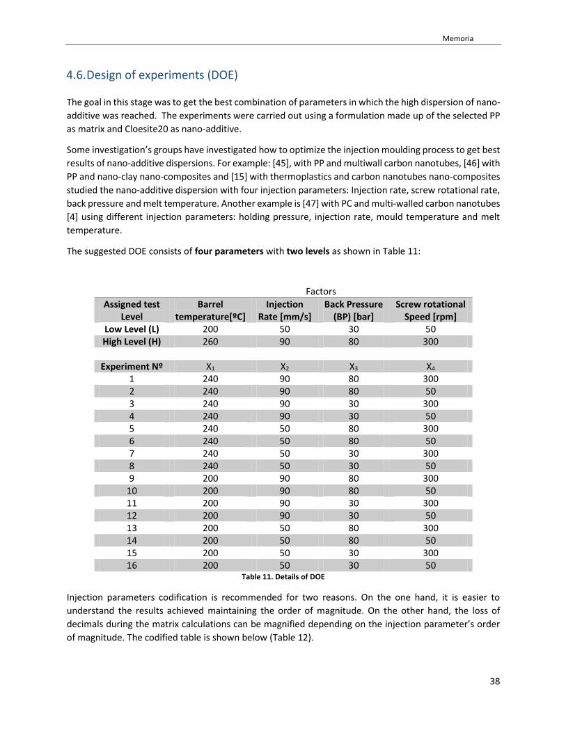
4.6. Design of experiments (DOE)

The goal in this stage was to get the best combination of parameters in which the high dispersion of nano-

additive was reached. The experiments were carried out using a formulation made up of the selected PP

as matrix and Cloesite20 as nano-additive.

Some investigation’s groups have investigated how to optimize the injection moulding process to get best

results of nano-additive dispersions. For example: [45], with PP and multiwall carbon nanotubes, [46] with

PP and nano-clay nano-composites and [15] with thermoplastics and carbon nanotubes nano-composites

studied the nano-additive dispersion with four injection parameters: Injection rate, screw rotational rate,

back pressure and melt temperature. Another example is [47] with PC and multi-walled carbon nanotubes

[4] using different injection parameters: holding pressure, injection rate, mould temperature and melt

temperature.

The suggested DOE consists of four parameters with two levels as shown in Table 11:

Factors

Assigned test Level

Barrel temperature[ºC]

Injection Rate [mm/s]

Back Pressure (BP) [bar]

Screw rotational Speed [rpm]

Low Level (L) 200 50 30 50 High Level (H) 260 90 80 300

Experiment Nº X1 X2 X3 X4

1 240 90 80 300 2 240 90 80 50 3 240 90 30 300 4 240 90 30 50 5 240 50 80 300 6 240 50 80 50 7 240 50 30 300 8 240 50 30 50 9 200 90 80 300

10 200 90 80 50 11 200 90 30 300 12 200 90 30 50 13 200 50 80 300 14 200 50 80 50 15 200 50 30 300 16 200 50 30 50

Table 11. Details of DOE

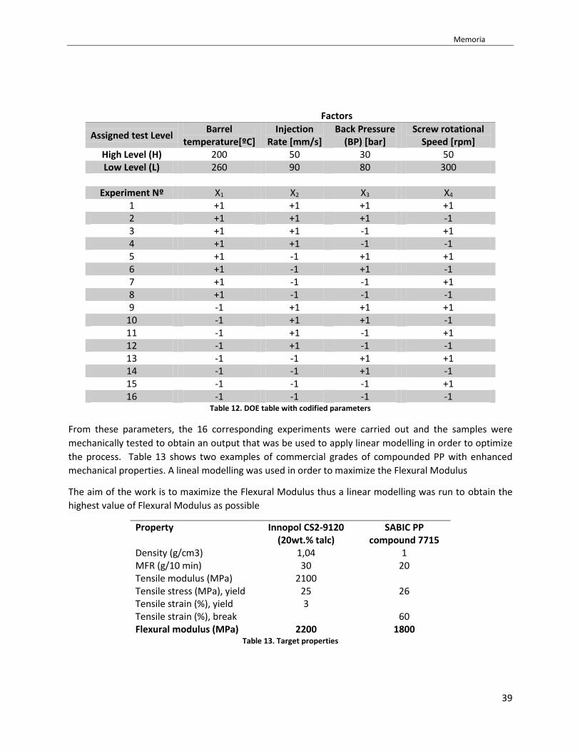
Injection parameters codification is recommended for two reasons. On the one hand, it is easier to

understand the results achieved maintaining the order of magnitude. On the other hand, the loss of

decimals during the matrix calculations can be magnified depending on the injection parameter’s order

of magnitude. The codified table is shown below (Table 12).

Memoria

39

Factors

Assigned test Level Barrel

temperature[ºC] Injection

Rate [mm/s] Back Pressure

(BP) [bar] Screw rotational

Speed [rpm] High Level (H) 200 50 30 50 Low Level (L) 260 90 80 300

Experiment Nº X1 X2 X3 X4

1 +1 +1 +1 +1 2 +1 +1 +1 -1 3 +1 +1 -1 +1 4 +1 +1 -1 -1 5 +1 -1 +1 +1 6 +1 -1 +1 -1 7 +1 -1 -1 +1 8 +1 -1 -1 -1 9 -1 +1 +1 +1

10 -1 +1 +1 -1 11 -1 +1 -1 +1 12 -1 +1 -1 -1 13 -1 -1 +1 +1 14 -1 -1 +1 -1 15 -1 -1 -1 +1 16 -1 -1 -1 -1

Table 12. DOE table with codified parameters

From these parameters, the 16 corresponding experiments were carried out and the samples were

mechanically tested to obtain an output that was be used to apply linear modelling in order to optimize

the process. Table 13 shows two examples of commercial grades of compounded PP with enhanced

mechanical properties. A lineal modelling was used in order to maximize the Flexural Modulus

The aim of the work is to maximize the Flexural Modulus thus a linear modelling was run to obtain the

highest value of Flexural Modulus as possible

Property Innopol CS2-9120 (20wt.% talc)

SABIC PP compound 7715

Density (g/cm3) 1,04 1 MFR (g/10 min) 30 20 Tensile modulus (MPa) 2100 Tensile stress (MPa), yield 25 26 Tensile strain (%), yield 3 Tensile strain (%), break 60 Flexural modulus (MPa) 2200 1800

Table 13. Target properties

Memoria

40

4.7. Lineal modelling

For the four selected parameters and two levels for each one, a lineal model has been used to determine

the effect of each parameter in the dispersion. The output for modelling was the Flexural Modulus and

the input was all 16 experiments. Five samples have been tested for each experiment getting a total of 80

flexural tests. General equation to solve for a lineal model was:

𝑌 = �̂�𝑋 → �̂� = (𝑋′𝑋)−1𝑋′𝑌 → �̂� = �̂�𝑋 (eq. 2)

Where:

𝑌 =

[ 𝑌1

𝑌2

𝑌3

⋮𝑌𝑛]

; 𝑋 =

[ 1 𝑋11 𝑋21 𝑋11𝑋21 𝑋𝑛𝑘

𝑚

1 𝑋11 𝑋22 … …

11⋮1

𝑋12

𝑋12

⋮𝑋1𝑘

𝑋21 … … 𝑋22 … …

⋮𝑋2𝑘

… …]

→ �̂� =

[ �̂�0

�̂�1

�̂�2

�̂�12

⋮�̂�𝑛 ]

(eq. 3)

�̂� is the output or response of the model

𝑋 is the input from all experiments (independent variables)

�̂� are the estimated coefficients

In this case, a first model was proposed taking into account all possible interactions between the selected

parameters:

�̂� = 𝛽0 + 𝛽1𝑋1 + 𝛽2𝑋2 + 𝛽3𝑋3 + 𝛽4𝑋4 + 𝛽12𝑋1𝑋2 + 𝛽13𝑋1𝑋3 + 𝛽14𝑋1𝑋4 + 𝛽23𝑋2𝑋3 + 𝛽24𝑋2𝑋4 (eq. 4)

Where:

𝛽0 is the origin de coordinates

𝛽1 coefficient related to barrel temperature

𝛽2 coefficient related to injection rate

𝛽3 coefficient related to back pressure

𝛽4 coefficient related to screw rotational rate

𝛽12 is related to interactions between 𝛽1and 𝛽2

𝛽13 is related to interactions between 𝛽1and 𝛽3

𝛽14 is related to interactions between 𝛽1and 𝛽4

𝛽23 is related to interactions between 𝛽2and 𝛽3

𝛽24 is related to interactions between 𝛽2and 𝛽4

Memoria

41

Scilab 6.0 was used to solve the matrix operations due the size of the matrix. The size of X was 80x10 and

�̂� was 80x1 and the resulting matrix �̂� was 10x1.

This model will only be valid and repeatable if the process has remained constant and has not changed its

conditions for data collection. Therefore, ensure that the configuration of the control parameters will not

affect the working conditions of the process, falsifying measured response. This is done via a study of

residuals, as well as verification of the significance of the model obtained.

4.8. Residuals

First step corresponds to verify the difference between the estimated response in a defined point and the

experimental responses obtained at the same point, known as residuals (𝜀 = �̂� − 𝑌) with 0 of average

and a constant variance (for every control factor) (Figure 20).

𝐻𝑦𝑝𝑜𝑡ℎ𝑒𝑠𝑖𝑠 1: 𝜀~𝑁(0, 𝜎2 = 𝑐𝑡)

Figure 19. Residuals of a normal experimental sample

To ensure this hypothesis, a test fit normal values of residues obtained has been performed.

The normal setting test is to perform a linear regression between the normal statistical standard (Z) and

the concerned values of the sorted residuals (ε). The normal statistical standard classification corresponds

to a supposed normal variable (ε) in a normal distribution equivalent on average zero and variance the

unit (Z):

𝜀~𝑁(𝑚 = 0; 𝜎2 = 𝑐𝑡) → 𝑍 =𝜀 − 𝑚

𝜎→ 𝑍~𝑁(0; 1)

(eq. 5)

Memoria

42

Figure 20. Residuals normal test

In Figure 20 is shown an example of residual normal test and in Figure 21 is shown an example of the

model.

Therefore, if the slope of the line obtained approximates the inverse of the standard deviation (σ),

estimated from the data, and the average calculated from the origin ordinate (m / σ) corresponds to the

value estimated from the data (in this case, should be 0), can be considered part of the first validated

hypotheses. Figure 22 shows the residual normal test for studied case.

Figure 21. Residual normal test for the third iteration of the model

Figure 22 confirmed that the variance remains constant for all control factors involved in the design of

experiments (k).

y = 0.028x - 2E-13R² = 0.9859

-3.00

-2.00

-1.00

0.00

1.00

2.00

3.00

-100.00 -80.00 -60.00 -40.00 -20.00 0.00 20.00 40.00 60.00 80.00 100.00

Z

e

Residual normal test

Memoria

43

To confirm this, the residual graphic is obtained for each control factors separately. If there is any trend

in terms of the extent of dispersion values or the variation of the average value for each factor level, it

can be confirmed that the residual corresponds to a normal random variable probability distribution, with

constant variance for all levels of control factors. Two extreme examples are shown in Figure 23.

Figure 22. Two examples of probability distribution. Left graph with constant variance and right graph with unstable variance

Figure 24 shows that residuals variance remains constant during all values.

Figure 23. Residual variance for the third iteration of the model

-100

-80

-60

-40

-20

0

20

40

60

80

100

1500 1600 1700 1800 1900 2000

e

Estimated Y

Variance residuals

Memoria

44

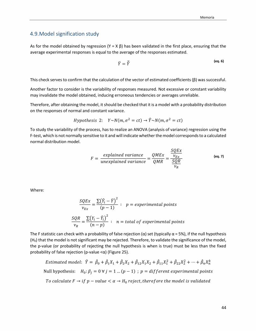
4.9. Model signification study

As for the model obtained by regression (Y = X β) has been validated in the first place, ensuring that the

average experimental responses is equal to the average of the responses estimated.

�̅� = �̅̂� (eq. 6)

This check serves to confirm that the calculation of the vector of estimated coefficients (β) was successful.

Another factor to consider is the variability of responses measured. Not excessive or constant variability

may invalidate the model obtained, inducing erroneous tendencies or averages unreliable.

Therefore, after obtaining the model, it should be checked that it is a model with a probability distribution

on the responses of normal and constant variance.

𝐻𝑦𝑝𝑜𝑡ℎ𝑒𝑠𝑖𝑠 2: 𝑌~𝑁(𝑚, 𝜎2 = 𝑐𝑡) → �̂�~𝑁(𝑚, 𝜎2 = 𝑐𝑡)

To study the variability of the process, has to realize an ANOVA (analysis of variance) regression using the

F-test, which is not normally sensitive to it and will indicate whether the model corresponds to a calculated

normal distribution model.

𝐹 = 𝑒𝑥𝑝𝑙𝑎𝑖𝑛𝑒𝑑 𝑣𝑎𝑟𝑖𝑎𝑛𝑐𝑒

𝑢𝑛𝑒𝑥𝑝𝑙𝑎𝑖𝑛𝑒𝑑 𝑣𝑎𝑟𝑖𝑎𝑛𝑐𝑒=

𝑄𝑀𝐸𝑥

𝑄𝑀𝑅=

𝑆𝑄𝐸𝑥𝜈𝐸𝑥

𝑆𝑄𝑅𝜈𝑅

(eq. 7)

Where:

𝑆𝑄𝐸𝑥

𝜈𝐸𝑥=

∑(�̂�𝑖 − �̅�)2

(𝑝 − 1) ∶ 𝑝 = 𝑒𝑥𝑝𝑒𝑟𝑖𝑚𝑒𝑛𝑡𝑎𝑙 𝑝𝑜𝑖𝑛𝑡𝑠

𝑆𝑄𝑅

𝜈𝑅=

∑(𝑌𝑖 − �̂�𝑖)2

(𝑛 − 𝑝) ∶ 𝑛 = 𝑡𝑜𝑡𝑎𝑙 𝑜𝑓 𝑒𝑥𝑝𝑒𝑟𝑖𝑚𝑒𝑛𝑡𝑎𝑙 𝑝𝑜𝑖𝑛𝑡𝑠

The F statistic can check with a probability of false rejection (α) set (typically α = 5%), if the null hypothesis

(H0) that the model is not significant may be rejected. Therefore, to validate the significance of the model,

the p-value (or probability of rejecting the null hypothesis is when is true) must be less than the fixed

probability of false rejection (p-value <α) (Figure 25).

𝐸𝑠𝑡𝑖𝑚𝑎𝑡𝑒𝑑 𝑚𝑜𝑑𝑒𝑙: �̂� = �̂�0 + �̂�1𝑋1 + �̂�2𝑋2 + �̂�12𝑋1𝑋2 + �̂�11𝑋12 + �̂�22𝑋2

2 + ⋯+ �̂�𝑛𝑋𝑛𝑘

Null hypothesis: 𝐻0: 𝛽𝑗 = 0 ∀ 𝑗 = 1… (𝑝 − 1) ; 𝑝 = 𝑑𝑖𝑓𝑓𝑒𝑟𝑒𝑛𝑡 𝑒𝑥𝑝𝑒𝑟𝑖𝑚𝑒𝑛𝑡𝑎𝑙 𝑝𝑜𝑖𝑛𝑡𝑠

𝑇𝑜 𝑐𝑎𝑙𝑐𝑢𝑙𝑎𝑡𝑒 𝐹 → 𝑖𝑓 𝑝 − 𝑣𝑎𝑙𝑢𝑒 < 𝛼 → 𝐻0 𝑟𝑒𝑗𝑒𝑐𝑡, 𝑡ℎ𝑒𝑟𝑒𝑓𝑜𝑟𝑒 𝑡ℎ𝑒 𝑚𝑜𝑑𝑒𝑙 𝑖𝑠 𝑣𝑎𝑙𝑖𝑑𝑎𝑡𝑒𝑑

Memoria

45

Figure 24. F or Snedecor probabilistic distribution

Once validated the significance of global model, the meaning of each of coefficients separately has been

studied because they may have terms that are not valid saturated model, so little impact on the decline,

inducing errors estimation and interpretation of the resulting function.

The T-test is a statistical tool that is commonly used for variables that follow normal distributions to

determine equality between different populations. In regressions can be used to determine the

significance of the various pending induced model of each term.

Therefore, it is defined as the null hypothesis (H0) that the value of the estimated coefficient (�̂�𝑗) can be

considered zero for each of the coefficients. The statistics associated T corresponds to the estimated

coefficient divided by the estimated variance (𝑆�̂�𝑗). In the same way that the test of hypothesis F must be

defined in a probability of false rejection (α, typically 5%). If the p-value (or probability of rejecting the

null hypothesis when is true) obtained is less than the probability of false rejection (p-value <α), we can

reject the null hypothesis a, and therefore accept meaning of the term in particular (¡Error! No se

encuentra el origen de la referencia.).

𝐸𝑠𝑡𝑖𝑚𝑎𝑡𝑒𝑑 𝑚𝑜𝑑𝑒𝑙: �̂� = �̂�0 + �̂�1𝑋1 + �̂�2𝑋2 + �̂�12𝑋1𝑋2 + �̂�11𝑋12 + �̂�22𝑋2

2 + ⋯ + �̂�𝑛𝑋𝑛𝑘

(eq. 8)

Null hypothesis: 𝐻0: 𝛽𝑗 = 0

(𝑓𝑜𝑟 𝑒𝑎𝑐ℎ 𝑐𝑜𝑒𝑓𝑓𝑖𝑐𝑖𝑒𝑛𝑡 𝑠𝑒𝑝𝑎𝑟𝑎𝑡𝑒𝑙𝑦, 𝑒𝑥𝑐𝑙𝑢𝑑𝑖𝑛𝑔 𝑡ℎ𝑒 𝑜𝑟𝑖𝑔𝑖𝑛 𝑜𝑟𝑑𝑖𝑛𝑎𝑡𝑒)

𝑆𝑡𝑎𝑡𝑖𝑐 𝑇 =�̂�𝑗

𝑆�̂�𝑗

(eq. 9)

Memoria

46

=�̂�𝑗

√𝑄𝑀𝑅 · 𝑑�̂�𝑗

; 𝑤ℎ𝑒𝑟𝑒 𝑑�̂�𝑗 𝑐𝑜𝑟𝑟𝑒𝑠𝑝𝑜𝑛𝑑𝑠 𝑡𝑜 𝑡ℎ𝑒 𝑡𝑒𝑟𝑚 𝑜𝑓 𝑡ℎ𝑒 𝑑𝑖𝑎𝑔𝑜𝑛𝑎𝑙 (𝑋′𝑋−1) 𝑎𝑠𝑠𝑜𝑐𝑖𝑎𝑡𝑒𝑑 𝑡𝑜 �̂�𝑗

𝑇𝑜 𝑐𝑎𝑙𝑐𝑢𝑙𝑎𝑡𝑒 𝑇 → 𝑖𝑓 𝑝 − 𝑣𝑎𝑙𝑢𝑒 < 𝛼 → 𝐻0 𝑟𝑒𝑗𝑒𝑐𝑡𝑒𝑑 , 𝑡ℎ𝑒𝑟𝑒𝑓𝑜𝑟 𝑡ℎ𝑒 𝑚𝑜𝑑𝑒𝑙 𝑖𝑠 𝑣𝑎𝑙𝑖𝑑𝑎𝑡𝑒𝑑

Figure 25. T or Student probabilistic distribution

The t-test was applied to each of the terms is not significant if any should be removed. As deleting a term

involves the modification of the model, always will be removed less significant term, and the model must

be re-calculated and re-validated, becoming an iterative process to get a model with all significant terms.

4.10. Model validation

Following the steps explained above, several iterations were carried out to validate the proposed model.

First model was calculated obtaining a matrix of 10 coefficients. The p column gives the p-value for each

coefficient. To ensure the model is consistent, p-value must be < 0.025 because α was considered 0.05.

Table 14 shows that there are p-values above the 0.025.

Coefficient β Diagonal (𝑿′𝑿) −𝟏 Error (Sβj ) T p

β0 1756,63 0,0125 5,944 β1 -112,88 0,0125 5,944 -18,991 0,000 β2 -2,13 0,0125 5,944 -0,358 0,722 β3 -1,38 0,0125 5,944 -0,231 0,818 β4 15,63 0,0125 5,944 2,629 0,010 β12 -53,63 0,0125 5,944 -9,022 0,000 β13 -15,38 0,0125 5,944 -2,587 0,012 β14 -18,38 0,0125 5,944 -3,092 0,003 β23 -1,63 0,0125 5,944 -0,273 0,785 β24 -13,63 0,0125 5,944 -2,292 0,025

Table 14. First model calculation

Memoria

47

First step consisted of deleting the highest value, which was related to β3. Next steps consisted of

recalculate the model without the rejected coefficient. This two steps will be carried out until all p-values

are below 0.025. Iterations are shown in Table 15 to Table 17.

Coefficient β Diagonal (𝑿′𝑿) −𝟏 Error (Sβj ) T p

β0 1760,92 0,013 4,181 β1 -108,58 0,013 4,181 -25,972 0,000 β2 2,17 0,013 4,181 0,519 0,605 β4 16,67 0,013 4,170 3,997 0,000 β12 -49,33 0,013 4,181 -11,799 0,000 β13 -1108,07 0,013 4,181 -265,041 0,000 β14 -17,33 0,013 4,170 -4,156 0,000 β23 2,67 0,013 4,181 0,638 0,525 β24 -12,58 0,013 4,170 -3,017 0,004

Table 15. Model validation's first iteration

Coefficient β Diagonal (𝑿′𝑿) −𝟏 Error (Sβj ) T p

β0 1760,82 0,013 4,189 β1 -108,68 0,013 4,189 -25,947 0,000 β4 16,71 0,013 4,178 3,999 0,000 β12 -49,43 0,013 4,189 -11,801 0,000 β13 -11,18 0,013 4,189 -2,670 0,009 β14 -17,29 0,013 4,178 -4,139 0,000 β23 2,57 0,013 4,189 0,613 0,542 β24 -12,54 0,013 4,178 -3,002 0,004

Table 16. Model validation's second iteration

Coefficient β Diagonal (𝑿′𝑿) −𝟏 Error (Sβj ) T p

β0 1760,70 0,013 4,200 β1 -108,80 0,013 4,200 -25,906 0,000 β4 16,75 0,013 4,189 3,999 0,000 β12 -49,55 0,013 4,200 -11,798 0,000 β13 -11,30 0,013 4,200 -2,690 0,009 β14 -17,25 0,013 4,189 -4,118 0,000 β24 -12,50 0,013 4,189 -2,984 0,004

Table 17. Model validation's third iteration

After all iterations, a consistent model was obtained. Note that some coefficient parameters or coefficient

interaction between parameter have been disappeared. The coefficients related to injection rate and back

pressure were deleted but remained in the interactions. The final model is shown below:

�̂� = 𝟏𝟕𝟔𝟎, 𝟕 − 𝟏𝟎𝟖, 𝟖𝐗𝟏 + 𝟏𝟔, 𝟕𝟔𝐗𝟒 − 𝟒𝟗, 𝟓𝟓𝐗𝟏𝐗𝟐 − 𝟏𝟏, 𝟑𝐗𝟏𝐗𝟑 − 𝟏𝟕, 𝟐𝟓𝐗𝟏𝐗𝟒 − 𝟏𝟐, 𝟓𝐗𝟐𝐗𝟒 (eq.10)

Memoria

48

4.11. Results

Once the model was solved, four response surfaces had been plotted. Each surface can represent 2 inputs

(i.e. injection rate and back pressure) and the behaviour of the two remaining related to the output can

be observed. An example is shown in Figure 26:

Figure 26. Example of a surface response

Note that the plot above has two variable parameters (melt temperature and injection rate) which varies

from -1 to +1 due to the codification. The other two parameters (back pressure and screw rotational rate)

have been fixed which in this case, are represented +1 for back pressure and +1 for screw rotational rate

(maximum level). All 16 response surfaces are shown in ¡Error! No se encuentra el origen de la

eferencia..

In one hand, if two parameters are fixed and two are variable, four combinations of them are possible.

On the other hand, 4 combinations between fixed and variable parameters are possible which results in

16 surfaces.

A summary of all combinations is shown in Table 18:

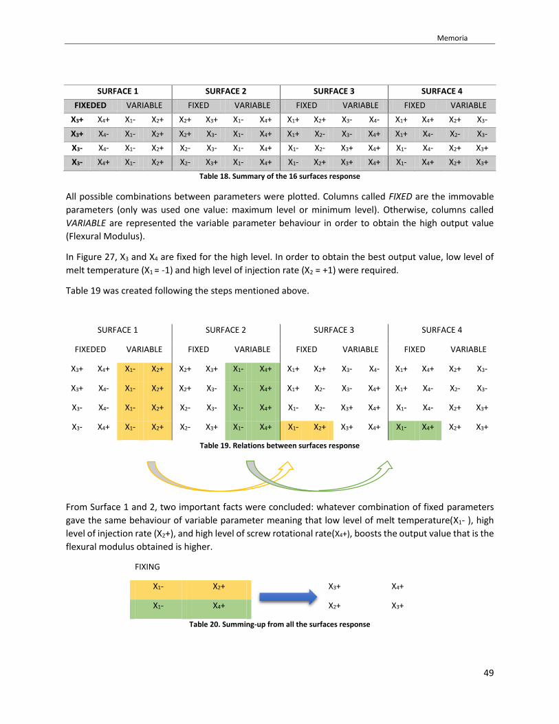
Memoria

49

SURFACE 1 SURFACE 2 SURFACE 3 SURFACE 4

FIXEDED VARIABLE FIXED VARIABLE FIXED VARIABLE FIXED VARIABLE

X3+ X4+ X1- X2+ X2+ X3+ X1- X4+ X1+ X2+ X3- X4- X1+ X4+ X2+ X3-

X3+ X4- X1- X2+ X2+ X3- X1- X4+ X1+ X2- X3- X4+ X1+ X4- X2- X3-

X3- X4- X1- X2+ X2- X3- X1- X4+ X1- X2- X3+ X4+ X1- X4- X2+ X3+

X3- X4+ X1- X2+ X2- X3+ X1- X4+ X1- X2+ X3+ X4+ X1- X4+ X2+ X3+

Table 18. Summary of the 16 surfaces response

All possible combinations between parameters were plotted. Columns called FIXED are the immovable

parameters (only was used one value: maximum level or minimum level). Otherwise, columns called

VARIABLE are represented the variable parameter behaviour in order to obtain the high output value

(Flexural Modulus).

In Figure 27, X3 and X4 are fixed for the high level. In order to obtain the best output value, low level of

melt temperature (X1 = -1) and high level of injection rate (X2 = +1) were required.

Table 19 was created following the steps mentioned above.

SURFACE 1 SURFACE 2 SURFACE 3 SURFACE 4

FIXEDED VARIABLE FIXED VARIABLE FIXED VARIABLE FIXED VARIABLE

X3+ X4+ X1- X2+ X2+ X3+ X1- X4+ X1+ X2+ X3- X4- X1+ X4+ X2+ X3-

X3+ X4- X1- X2+ X2+ X3- X1- X4+ X1+ X2- X3- X4+ X1+ X4- X2- X3-

X3- X4- X1- X2+ X2- X3- X1- X4+ X1- X2- X3+ X4+ X1- X4- X2+ X3+

X3- X4+ X1- X2+ X2- X3+ X1- X4+ X1- X2+ X3+ X4+ X1- X4+ X2+ X3+

Table 19. Relations between surfaces response

From Surface 1 and 2, two important facts were concluded: whatever combination of fixed parameters

gave the same behaviour of variable parameter meaning that low level of melt temperature(X1- ), high

level of injection rate (X2+), and high level of screw rotational rate(X4+), boosts the output value that is the

flexural modulus obtained is higher.

FIXING

X1- X2+ X3+ X4+

X1- X4+ X2+ X3+

Table 20. Summing-up from all the surfaces response

Memoria

50

5. Conclusions

Scientific Injection Molding is a tool that should be used for every mold set-up in order to ensure the best

performance during the injection molding process. It allows to study the most significant parameters

taking into account the IMM, the tool features and the rheology of the material used for each specific

case. Minimal variation on the system i.e. material batch variation, gate tool, etc. will require a new

iteration of the SIM steps. Therefore, this project is focused on a specific system but may be useful as a

guideline for another system.

1. Four parameters have been studied to see the significance of them into the mechanical properties

of the final part. In this case, the target properties was Flexural Modulus of a standard specimen

and depends on the application of the injected part, different property could be studied.

2. After the model was calculated and validated some trends were obtained. High values of back

pressure, screw rotational speed and injection speed boosted the output of the model (Flexural

Modulus) while low values of melt temperature also boosted the Flexural Modulus.

3. On one hand, high values of back pressure and screw rotational speed may maintain or improve

the dispersion achieved during the extrusion compounding. High injection rate may aid the

additives orientation and then keep them homogenous.

4. On the other hand, at first sight, high melt temperature should improve the nano-additives

mobility but in this case, high temperature and then high viscosity may ease the nano-additive re-

aggregation and then reduce the mechanical.

5. To sum up, low values of melt temperature and high values of injection rate, back pressure and

screw rotational speed will be required to achieve high values of Flexural Modulus.

Memoria

51

Memoria

52

6. References

[1] “https://www.plasticseurope.org,” [Online].

[2] P. E. P. E. a. T. H. H. Domininghaus, Kunststoffe: Eigenschaften und Anwendungen ; mit 240 Tabellen,

Springer-Verlag GmbH, 2008.

[3] D. Braun, Kunststofftechnik für Einsteiger, Hanser, 2003.

[4] W. Kaiser, Kunststoffchemie für Ingenieure, Hanser Fachbuchverlag, 2007.

[5] D. L. H. D. C. S. K. J. L. W. J. W. C. e. a. H. R. Dennis, “Effect of melt processing conditions on the

extent of exfoliation in organoclay-based nanocomposites,” Polymer, vol. 42, pp. 9513-9522, 2001.

[6] N. E. H. J. J. L. a. R. A. P. C. P. McAdam, “Synthesis and characterization of nylon 6/clay

nanocomposites prepared by ultrasonication and in situ polymerization,” Journal of Applied Polymer

Science, vol. 108, pp. 2242-2251, 2008.

[7] R. K. S. D. L. H. a. D. R. P. F. Chavarria, “Effect of melt processing conditions on the morphology and

properties of nylon 6 nanocomposites,” Polymer Engineering and Science, vol. 47, pp. 1847-1864,

2007 xxxxx.

[8] D. R. P. a. L. M. Robeson, “Polymer nanotechnology: Nanocomposites,” Polymer, vol. 49, pp. 3187-

3204, 2008.

[9] S. K. S. a. A. I. I. S. Lapshin, “Ultrasound aided extrusion process for preparation of polyolefin-clay

nanocomposites,” Polymer Engineering and Science, vol. 48, pp. 1584-1591, 2008.

[10] E. Bugnicourt, “Development of sub-micro structured composites based on an epoxy matrix and

pyrogenic silica: mechanical behavior related to the interactions and morphology at multi-scale,”

Villeurbanne, INSA, 2005.

[11] S. P. P. P. a. U. W. T. Villmow, “Influence of injection molding parameters on the electrical resistivity

of polycarbonate filled with multi-walled carbon nanotubes,” Composites Science and Technology,

vol. 68, pp. 777-789, 2008.

[12] A. J. K. X. H. a. L. S. T. A. Chandra, "Effect of injection molding parameters on the electrical

conductivity of polycarbonate/carbon nanotube nanocomposites," in Annual Technical Conference

- ANTEC, 2007.

[13] L. I. S. a. C. F. F. Stan, “Effect of processing parameters and strain rate on mechanical properties of

carbon nanotube-filled polypropylene nanocomposites,” Composites Part B-Engineering, vol. 59, pp.

109-122, 2014.

Memoria

53

[14] V. P. J. V. A. P. A. P. a. P. F. A. Costantino, “Microstructure of PP/clay nanocomposites produced by

shear induced injection moulding,” in 11th International Congress on Metallurgy & Materials, 2011.

[15] P. F. Rios, A. Ophir, S. Kenig, R. Efrati, L. Zonder and R. Popovitz-Biro., "Impact of injection-moulding

processing parameters on the electrical, mechanical, and thermal properties of

thermoplastic/carbon nanotube nanocomposites.," 11th October 2010. [Online]. [Accessed 7th

January 2018].

[16] M. Okamoto, “Recent advances in polymer/layered silicate nanocomposites: an overview from

science to technology,” Materials Science and Technology , vol. 22, no. 7, pp. 756-779 , 2006.

[17] J. Zhang, E. Manias and C. A. Wilkie, "Polymerically Modified Layered Silicates: An Effective Route to

Nanocomposites," Journal of Nanoscience and Nanotechnology, vol. 8, no. 4, pp. 1597-1615, 2008.

[18] C. D. P. S. Pavlidou, “A review on polymer–layered silicate nanocomposites,” Progress in Polymer

Science, vol. 33, no. 12, pp. 1119-1198, 2008.

[19] p. a. u. o. a. n. c. o. m. Polymer-layered silicate nanocomposites: preparation, “Michael Alexandre,

Philippe Dubois,” Polymer-layered silicate nanocomposites: preparation, properties and uses of a

new class of materials, vol. 28, no. 1-2, pp. 1-63, 2000.

[20] A. K. B. C. O. Anusuya Choudhury, “Novel role of polymer–solvent and clay–solvent interaction

parameters on the thermal, mechanical and optical properties of polymer nanocomposites,”

Polymer, vol. 50, no. 1, pp. 201-210, 2009.

[21] H. H.Murray, “Overview — clay mineral applications,” Applied Clay Science, vol. 5, no. 5-6, pp. 379-

395, 1991.

[22] [Online]. Available: www.moldedfiberglass.com/library/news/newsCW8-09.pdf.

[23] J. G. H. D. S. B. L.W Carter, "Elastomer Reinforced with a Modified Clay". US Patent 2,531,396, 1950.

[24] P. G. N. a. P. S. Backlund, "Organoclay-Polyolefin Compositions". US Patent 3,084,117, 1963.

[25] T. S. S. Fujiwara, “Method for Manufacturing a Clay/Polyamide Composite”. Japanese Kokai Patent

Application Patent 109,998, 1976.

[26] Y. F. a. S. Inagaki, “Synthesis of an Intercalated Compound of Montmorillonite and 6-Polyamide,”

Journal of Inclusion Phenomena, vol. 5, pp. 473-482, 1987.

[27] Y. K. M. K. A. O. Y. F. T. K. a. O. K. A. Usuki, “Synthesis of Nylon 6–Clay Hybrid,” Journal of Materials

Research, no. 8, pp. 1179-1184, 1993.

[28] T. M. Y. F. M. F. K. F. Y. K. ,. N. T. K. a. O. K. A. Usuki, “Composite Material containing a Layered

Silicate”. US Patent 4,889,885, 1989.

Memoria

54

[29] Y. K. e. al., “Sorption of Water in Nylon 6-clay Hybrid,” Journal of Applied Polymer Science, no. 4, pp.

1259-1264, 1993.

[30] K. F. A. U. Y. K. N. S. T. K. a. O. K. A. Okada, “Rubber-Clay Hybrid-Synthesis and Properties,” ACS Polym

Preprints, no. 32, pp. 540-541, 1991.

[31] A. U. A. Okada, “The Chemistry of Ppolymer-Clay Hybrids,” Materials Science and Engineering, no. C

3, pp. 109-115, 1995.

[32] K. Y. K. U. A. O. a. A. T. Kurauch, “Polyimide Composite Material and Process for Producing the

Same”. US Patent 5,164,46, 17 Nov 1992.

[33] A. U. a. A. O. K. Yano, “Synthesis and Properties of Polyimide-Clay Hybrid Films,” Journal of Applied

Polymer Science: Part A, Polym Chem., no. 35, pp. 2289-2294, 1997.

[34] F. Gao, “Clay/Polymer Composites:The Story,” Materials Today, no. 7, pp. 50-55, 2004.

[35] C. Edser, “Auto Applications of Drive Commercialization of Nanocomposites,” Plastic Additives

Compounding, no. 4, pp. 30-33, 2002.

[36] A. O. T. N. T. N. S. S. a. R. D. T. Kurauchi, “Nylon 6-Clay Hybrid - Synthesis, Properties and Application

to Automotive Timing Belt Cover,” SAE Technical Paper Ser, 910584, 1991.

[37] e. a. H.Cox, “Nanocomposite Systems for Automotive Applications,” in 4th World Congress in

Nanocomposites, EMC, San Francisco, 2004.

[38] M. N. J. B. Q.Z. Zhao, “Ultimate Strength of Carbon nanotubes: A Theoretical Study,” Phys. Rev. B,

no. 65, 2002.

[39] B. O. I. A. R. R. a. D. A. R. Prud'homme, “"Functional Graphene–Rubber Nanocomposites"”. US Patent

7,745,528, 29 Jun 2010.

[40] B. Z. J. Aruna Zhamu, “Pristine Nano Graphene-Modified Tires”. US Patent 7,999,027, 16 Aug 2011.

[41] S. B. A. S. N. Tahmassebi, "Effect of addition of hydrophobic nano silica on viscoelastic properties

and scratch resistance of an acrylic/melamine automotive clearcoat," TribologyInternational, no. 43,

p. 685–693, 2010.

[42] S. R. Zahra Ranjbara, “Nano mechanical properties of an automotive clear-coats containing nano

silica,” Progress in Organic Coatings, no. 72, pp. 40-43, 2011.

[43] M. M. M. M. Z. R. H. Yari, “Tribological properties and scratch healing of a typical automotive nano

clearcoat modified by a polyhedral oligomeric silsesquioxane compound,” European Polymer

Journal, no. 60, pp. 79-91, 2014.

[44] A. K. M. H. L. T. D. G. B. Ermias G Koricho1, “Effect of hybrid (micro- and nano-) filler on impact

response of GFRP composite,” Composite Structures, 2015.

Memoria

55

[45] K. Prashantha, J. Soulestin, M. F. Lacrampe, E. Lafranche, P. Krawczak, G. Dupin and M. Claes.,

"Taguchi analysis of shrinkage and warpage ofinjection-moulded polypropylene/multiwall carbon

nanotubes nanocomposites.," eXPRESS Polymer Letters, pp. 630-638, 2009.

[46] J. J. Rajesh, J. Soulestin, M. F. Lacrampe and P. Krawczak., "Effect of injection moulding parameters

on nanofillers dispersion in masterbatch based PP-clay nanocomposites.," eXPRESS Polymer Letters

Vol.6, p. 237–248, 2012.

[47] T. Villmow, S. Pegel, P. Pötschke and U. Wagenknecht., "Influence of injection moulding parameters

on the electrical resistivity of polycarbonate filled with multi-walled carbon nanotubes.," Composites

Science and Technology 68, p. 777–789, 2008.

[48] S. Kulkarni, Robust Process Development. Theory and Practice, Munich: Hanser, 2010.

[49] P. Dominick V. Rosato, Plastic Processing Data Handbook,, Second ed., Chatham, MA, 02633:

Chapman & Hall, 1997.

[50] D. M. Bryce, Plastic Injection Molding, vol. Manufacturing process fundamentals, Dearborn,

Michigan: Society of Manufacturing Engineers, 1996.

Memoria

56

7. Annex

7.1. Annex 1. Surface responses

All surfaces response are shown as a result of the mathematical model in this annex.

Figure 27. Surface response 1. Fixed parameters: Back pressure and Screw rotational rate. Variable parameters: Melt

temperature and Injection rate.

Memoria

57

Figure 28. Surface response 2. Fixed parameters: Back pressure and Screw rotational rate. Variable parameters: Melt

temperature and Injection rate.

Figure 29. Surface response 3. Fixed parameters: Back pressure and Screw rotational rate. Variable parameters: Melt

temperature and Injection rate.

Memoria

58

Figure 30. Surface response 4. Fixed parameters: Back pressure and Screw rotational rate. Variable parameters: Melt

temperature and Injection rate.

Figure 31. Surface response 5. Fixed parameters: Back pressure and injection rate. Variable parameters: Melt temperature

and screw rotational rate.

Memoria

59

Figure 32. Surface response 6. Fixed parameters: Back pressure and injection rate. Variable parameters: Melt temperature

and screw rotational rate.

Figure 33. Surface response 7. Fixed parameters: Back pressure and injection rate. Variable parameters: Melt temperature

and screw rotational rate.

Memoria

60

Figure 34. Surface response 8. Fixed parameters: Back pressure and injection rate. Variable parameters: Melt temperature

and screw rotational rate.

Figure 35. Surface response 9. Fixed parameters: Injection rate and melt temperature. Variable parameters: back pressure

and screw rotational rate.

Memoria

61

Figure 36. Surface response 10. Fixed parameters: Injection rate and melt temperature. Variable parameters: back pressure

and screw rotational rate.

Figure 37. Surface response 11. Fixed parameters: Injection rate and melt temperature. Variable parameters: back pressure

and screw rotational rate.

Memoria

62

Figure 38. Surface response 12. Fixed parameters: Injection rate and melt temperature. Variable parameters: back pressure

and screw rotational rate.

Figure 39. Surface response 13. Fixed parameters: Screw rotational rate and melt temperature. Variable parameters:

injection rate and back pressure.

Memoria

63

Figure 40. Surface response 14. Fixed parameters: Screw rotational rate and melt temperature. Variable parameters:

injection rate and back pressure.

Figure 41. Surface response 15. Fixed parameters: Screw rotational rate and melt temperature. Variable parameters:

injection rate and back pressure

Memoria

64

Figure 42. Surface response 16. Fixed parameters: Screw rotational rate and melt temperature. Variable parameters:

injection rate and back pressure.