InnoALM:

An Innovest Austrian Pension Fund

Financial Planning Model

William T. Ziemba

University of British Columbia

Joint paper with

Alois Geyer, University of Economics, Vienna, Austria

Wolfgang Herold and Konrad Kontriner, Innovest, Vienna, Austria

2

What is InnoALM?

• A multi-period stochastic linear programming model designed byZiemba and implemented by Geyer with input from Herold andKontriner

• For Innovest to use for Austrian pension funds

• A tool to analyze Tier 2 pension fund investment decisions

Why was it developed?

• To respond to the growing worldwide challenges of ageingpopulations and increased number of pensioners who put pressureon government services such as health care and Tier 1 nationalpensions

• To keep Innovest competitive in their high level fund managementactivities

Features of InnoALM

• A multiperiod stochastic linear programming framework with aflexible number of time periods of varying length.

• Generation and aggregation of multiperiod discrete probabilityscenarios for random return and other parameters

• Various forecasting models

• Scenario dependent correlations across asset classes

• Multiple co-variance matrices corresponding to differing marketconditions

• Constraints reflect Austrian pension law and policy

3

Technical features include:

• Concave risk averse preference function maximizes expectedpresent value of terminal wealth net of expected convex (piecewiselinear) penalty costs for wealth and benchmark targets in eachdecision period.

• InnoALM user interface allows for visualization of key modeloutputs, the effect of input changes, growing pension benefits fromincreased deterministic wealth target violations, stochasticbenchmark targets, security reserves, policy changes, etc.

• Solution process using the IBM OSL stochastic programming codeis fast enough to generate virtually online decisions and results andallows for easy interaction of the user with the model to improvepension fund performance.

InnoALM anticipates and reacts to all market conditions:severe as well as normal

4

Description of the Pension Fund

Siemens AG Österreich is the largest privately owned industrialcompany in Austria. Turnover (EUR 2.4 Bn. in 1999) is generated ina wide range of business lines including information andcommunication networks, information and communication products,business services, energy and traveling technology, and medicalequipment.

• The Siemens Pension fund, established in 1998, is the largestcorporate pension plan in Austria and follows the definedcontribution principle.

• More than 15.000 employees and 5.000 pensioners are members ofthe pension plan with about EUR 500 million in assets undermanagement.

• Innovest Finanzdienstleistungs AG, which was founded in 1998,acts as the investment manager for the Siemens AG Österreich, theSiemens Pension Plan as well as for other institutional investors inAustria.

• With EUR 2.2 billion in assets under management, Innovestfocuses on asset management for institutional money and pensionfunds.

• The fund was rated the 1st of 19 pension funds in Austria for thetwo-year 1999/2000 period

5

Factors that led Innovest to develop the pension fund asset-liability management model InnoALM.

• Changing demographics in Austria, Europe and the rest of theglobe, are creating a higher ratio of retirees to working population.

• Growing financial burden on the government making it paramountthat private employee pension plans be managed in the bestpossible way using systematic asset-liability management modelsas a tool in the decision making process.

• A myriad of uncertainties, possible future economic scenarios,stock, bond and other investments, transactions costs and liquidity,currency aspects, liability commitments

• Both Austrian pension fund law and company policy suggest thatmultiperiod stochastic linear programming is a good way to modelthese uncertainties.

• Faster computers have been a major factor in the development anduse of such models, SP problems with millions of variables havebeen solved by my students Edirisinghe and Gassmann and bymany others such as Dempster, Gonzio, Kouwenberg, Mulvey,Zenios, etc

• Good user friendly models now need to be developed that wellrepresent the situation at hand and provide the essentialinformation required quickly to those who need to make soundpension fund asset-liability decisions.

InnoALM and other such models allow pension funds to strategicallyplan and diversify their asset holdings across the world, keeping trackof the various aspects relevant to the prudent operation of a companypension plan that is intended to provide retired employees asupplement to their government pensions.

6

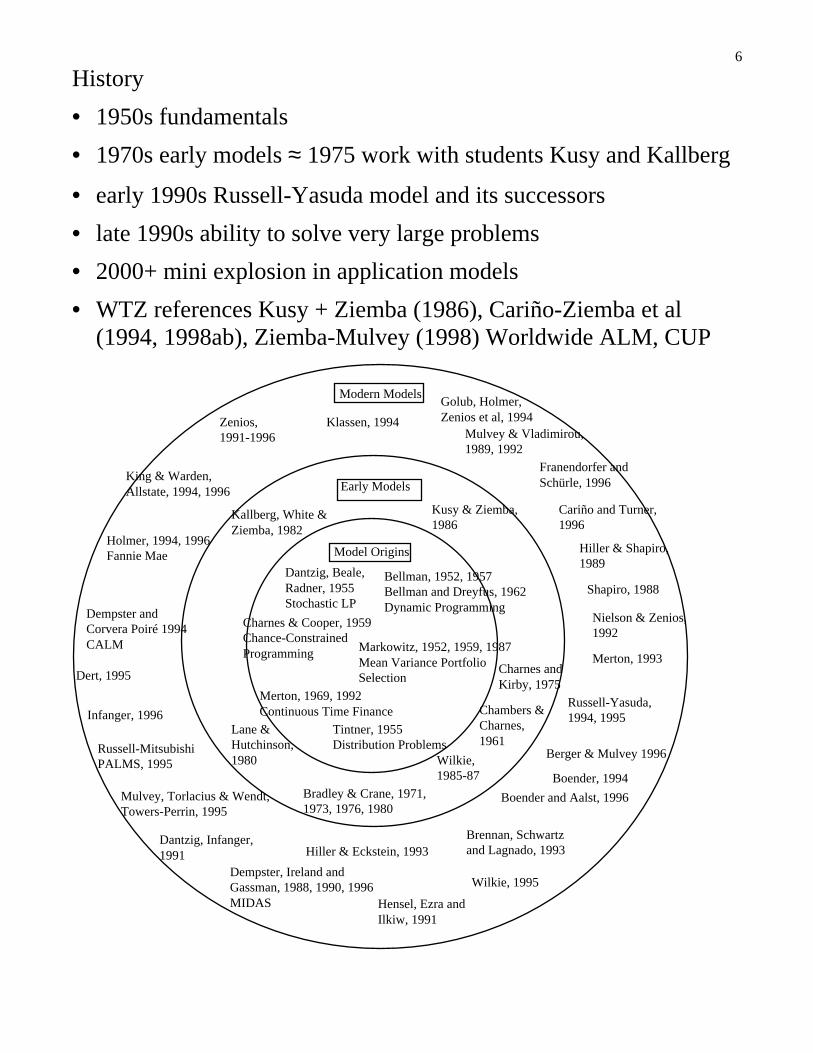
History

• 1950s fundamentals

• 1970s early models ≈ 1975 work with students Kusy and Kallberg

• early 1990s Russell-Yasuda model and its successors

• late 1990s ability to solve very large problems

• 2000+ mini explosion in application models

• WTZ references Kusy + Ziemba (1986), Cariño-Ziemba et al(1994, 1998ab), Ziemba-Mulvey (1998) Worldwide ALM, CUP

Dantzig, Beale, Radner, 1955Stochastic LP

Tintner, 1955Distribution Problems

Bellman, 1952, 1957Bellman and Dreyfus, 1962Dynamic Programming

Charnes & Cooper, 1959Chance-Constrained Programming Markowitz, 1952, 1959, 1987

Mean Variance Portfolio Selection

Bradley & Crane, 1971, 1973, 1976, 1980

Kallberg, White & Ziemba, 1982

Kusy & Ziemba, 1986

Early Models

Model Origins

Modern Models

Dempster, Ireland and Gassman, 1988, 1990, 1996MIDAS

Brennan, Schwartz and Lagnado, 1993

Mulvey & Vladimirou, 1989, 1992

Hiller & Shapiro, 1989

Nielson & Zenios, 1992

Merton, 1993

Russell-Yasuda, 1994, 1995

Berger & Mulvey 1996

Boender and Aalst, 1996

Zenios, 1991-1996

King & Warden, Allstate, 1994, 1996

Holmer, 1994, 1996 Fannie Mae

Dert, 1995

Infanger, 1996

Russell-Mitsubishi PALMS, 1995

Mulvey, Torlacius & Wendt, Towers-Perrin, 1995

Golub, Holmer, Zenios et al, 1994Klassen, 1994

Franendorfer and Schürle, 1996

Dantzig, Infanger, 1991 Hiller & Eckstein, 1993

Wilkie, 1985-87

Dempster and Corvera Poiré 1994CALM

Hensel, Ezra and Ilkiw, 1991

Cariño and Turner, 1996

Charnes and Kirby, 1975

Boender, 1994

Wilkie, 1995

Shapiro, 1988

Merton, 1969, 1992 Continuous Time Finance

Lane & Hutchinson, 1980

Chambers & Charnes, 1961

7

Advantages of Multiperiod Stochastic Programming Approach

• This approach has a number of practical advantages overalternative approaches for asset & liability management as staticmean-variance analysis (Sharpe and Tint, 1990), continuous timemodeling (Rudolf and Ziemba, 2000), shortfall risk minimization(Leibowitz and Henriksson, 1988) and other approaches (Ziembaand Mulvey, 1998 and Samuelson, 1989).

• This approach includes more of the essential elements of the realproblem.

• Insight follows from the study of alternative approaches and muchof that theory is embedded in InnoALM.

• Ex post studies of pension fund performance over time such asBrinson, Hood and Beebower (1986), Hensel, Ezra and Iikiw(1991) and Blake, Lehmann and Timmermann (1999) focus onvarious possible sources of performance enhancement such asstrategic asset allocation, market timing and security selection.

• These studies indicate that strategic asset allocation is the crucialvariable in successful pension fund performance.

InnoALM provides a good procedure for implementing crucialaspects of pension fund management policies, constraints and goalsto achieve superior long run performance while at the same timeproviding short-term risk management through diversification acrossvarious scenarios.

8

Project Team

• For the Russell Yasuda-Kasai model, we had a very large team andoverhead cost was very high.

• At Innovest we were a team of four with Geyer implementing myideas with Herold and Kontriner contributing guidance andinformation about the Austrian situation.

• The IBM OSL Stochastic Programming Code of Alan King wasused with various interfaces allowing lower development costs[for a survey of codes see in forthcoming Wallace-Ziemba book,Applications of Stochastic Programming, a friendly users guide toSP modeling, computations and applications, SIAM MPS]

The success of InnoALM demonstrates that a small team ofresearchers with a limited budget can quickly produce a valuablemodeling system that can easily be operated by non-stochasticprogramming specialists on a single PC.

9

The Pension Fund Situation in Austria and Europe

• Rapid ageing of the developed world’s populations - the retireegroup, those 65 and older, will roughly double from about 20% toabout 40% of compared to the worker group, those 15-64

• Better living conditions, more effective medical systems, a declinein fertility rates and low immigration into the Western worldcontribute to this ageing phenomenon.

• By 2030 two workers will have to support each pensionercompared with four now.

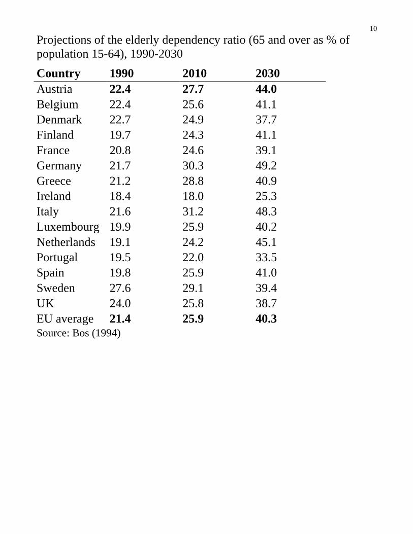
10

Projections of the elderly dependency ratio (65 and over as % ofpopulation 15-64), 1990-2030

Country 1990 2010 2030Austria 22.4 27.7 44.0Belgium 22.4 25.6 41.1Denmark 22.7 24.9 37.7Finland 19.7 24.3 41.1France 20.8 24.6 39.1Germany 21.7 30.3 49.2Greece 21.2 28.8 40.9Ireland 18.4 18.0 25.3Italy 21.6 31.2 48.3Luxembourg 19.9 25.9 40.2Netherlands 19.1 24.2 45.1Portugal 19.5 22.0 33.5Spain 19.8 25.9 41.0Sweden 27.6 29.1 39.4UK 24.0 25.8 38.7EU average 21.4 25.9 40.3Source: Bos (1994)

11

EU State pensions (pillar 1) are about 88% of total pension costs.

• Demographics will have a major impact on public and privatepension plans in Europe.

• Without a change in the policy towards financing methods ofpension expenditures, future costs will increase significantly -especially in the public social security systems, which are usuallybased on the pay-as-you-go principle,.

• Without any changes the pension payouts will grow from 10% ofGDP in 1997 to over 15% of GDP in 2030 for many EU countries.

• Contribution rates must be raised significantly to enable the publicsocial security system to cope with this problem.

In the UK and Ireland, pension costs will remain stable over theprojection period.

• These countries have pension schemes linked to employment(second pillar) and pension provisions taken out by individuals(third pillar) are well established.

12

OECD projections of pension costs, Pension expenditure/GDP

1995 2000 2010 2020 2030 2040Belgium 10.4 9.7 8.7 10.7 13.9 15.0Denmark 6.8 6.4 7.6 9.3 10.9 11.6Finland 10.1 9.5 10.7 15.2 17.8 18.0France 10.6 9.8 9.7 11.6 13.5 14.3Germany 11.1 11.5 11.8 12.3 16.5 18.4Ireland 3.6 2.9 2.6 2.7 2.8 2.9Italy 13.3 12.6 13.2 15.3 20.3 21.4Netherlands 6.0 5.7 6.1 8.4 11.2 12.1Portugal 7.1 6.9 8.1 9.6 13.0 15.2Spain 10.0 9.8 10.0 11.3 14.1 16.8Sweden 11.8 11.1 12.4 13.9 15.0 14.9UK 4.5 4.5 5.2 5.1 5.5 5.0Source: Rosevaere et al. (1996)

13

Pension fund assets as a percent of GDP are rather low, except forthe UK, the Netherlands and to a lesser extent Ireland and Sweden.

• In 1997 only 7% of total pension payments for the whole EUwere from pillar two and less from pillar three.

• The Netherlands (32%) and the UK (28%) have more developedprivate pension fund systems.

• In Austria they were less than half of the EU average at barely10% of GDP.

Pension Fund Assets as a percentage of GDP in 1997, in bn. ECU

Countries Assets GDP as a % of GDPAustria 20.9273 181.8278 11.51Belgium 10.3493 213.8373 4.84Denmark 29.3019 143.7339 20.39Finland 8.8766 103.6119 8.57France 84.4193 1,229.0572 6.87Germany 270.7216 1,865.3663 14.51Greece 4.5854 105.0228 4.37Ireland 34.4642 64.1071 53.76Italy 21.5814 1,010.7227 2.14Luxembourg 0.0283 13.6679 0.21Netherlands 361.6643 320.0063 113.02Portugal 9.3663 85.9758 10.89Spain 18.6856 470.3538 3.97Sweden 96.1839 202.3738 47.53U.K. 891.2270 1,127.2971 79.06

Total EU 1,862.3823 7,136.9617 26.09Source: European Federation for Retirement Provision (EFRP) (1996)

14

Effective private pension plans will need to play a more major rolegiven the countries’ demands for health care and other social servicesin addition to pensions.

• Reforms of the public pension systems will be necessary alongwith an effective environment for pillar 2 and 3 private pensionsystems.

InnoALM is a model for the effective operation of second pillarprivate pension funds in Austria.

• These funds usually work on a funded basis where the pensionbenefits depend on an employment contract or the pursuit of aparticular profession.

• Schemes are administered by private institutions.

• Benefits are not guaranteed by the state.

• Employer pension schemes vary throughout Europe.

• Contributions to such systems are made by the employer and, onan optional basis, by employees.

• The contribution level may depend on the wage level or theposition within a company.

• Defined contribution plans (DCP), have fixed contributions and thepayout depends on the capital accumulation of the plan. Definedbenefit plans (DBP) have payouts guaranteed by the company andthe contribution is variable depending on the capital accumulationover time.

15

Risk Bearer

In DBP’s, the employer guarantees the pension payment - usuallytied to some wage at or near retirement.

• If asset returns do not cover pension liabilities, the companywould have to inject money into the pension plan.

• If asset returns of the plan are higher than required to fundliabilities, the company would gain, or equivalently reduce futurecontributions.

For DCPs, employees and pensioners bear the risk of low assetreturns.

• Their pensions are not fixed and depend on the asset returns.

• High returns will increase pensions and vice versa.

• There is no direct financial risk for the employer although withpoor returns the employer would suffer negative image effects.

• The Siemens pension plan for Austria is a DCP but InnoALM isdesigned to handle either pension system.

16

Examples of national investment restrictions on pension plans

Country Investment Restrictions

Germany Max. 30% equities, max. 5% foreign bonds

Austria Max. 40% equities, max. 45% foreign securities,min. 40% EURO bonds

France Min. 50% EURO bonds

Portugal Max. 35% equities

Sweden Max. 25% equities

UK, US Prudent man rule

Source: European Commission (1997)

In new proposals, the limit for worldwide equities would rise to 70%versus the current average of about 35% in EU countries.

17

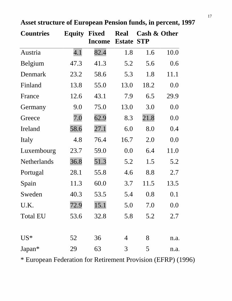
Asset structure of European Pension funds, in percent, 1997

Countries Equity FixedIncome

RealEstate

Cash &STP

Other

Austria 4.1 82.4 1.8 1.6 10.0

Belgium 47.3 41.3 5.2 5.6 0.6

Denmark 23.2 58.6 5.3 1.8 11.1

Finland 13.8 55.0 13.0 18.2 0.0

France 12.6 43.1 7.9 6.5 29.9

Germany 9.0 75.0 13.0 3.0 0.0

Greece 7.0 62.9 8.3 21.8 0.0

Ireland 58.6 27.1 6.0 8.0 0.4

Italy 4.8 76.4 16.7 2.0 0.0

Luxembourg 23.7 59.0 0.0 6.4 11.0

Netherlands 36.8 51.3 5.2 1.5 5.2

Portugal 28.1 55.8 4.6 8.8 2.7

Spain 11.3 60.0 3.7 11.5 13.5

Sweden 40.3 53.5 5.4 0.8 0.1

U.K. 72.9 15.1 5.0 7.0 0.0

Total EU 53.6 32.8 5.8 5.2 2.7

US* 52 36 4 8 n.a.

Japan* 29 63 3 5 n.a.

* European Federation for Retirement Provision (EFRP) (1996)

18

Why do European pensions invest so much in bonds?

• More “mature” pillar 2 countries such as the UK and Ireland,which have managed portfolios for outside investors for a longtime, have a higher equity exposure which may better reflect thelong term aspect of pension obligations.

• In countries like Austria, Germany, Italy, Spain and France equitymarkets that were not developed until recently have pension plansthat are invested more in local government bonds.

• Such asset structures reflect the attitude towards equities in variouscountries.

• The introduction of the EURO in 1999 is a first important steptowards a more integrated capital market, especially for equities.

• In Austria, pension funds are now starting to increase their equitypositions, but it will take some time to reach a structure similar tothose in well established US, UK and Irish pension industries.

• Strict regulations, lack of investment products, fear of foreigninvestment, a short term outlook, and traditional investmentbehavior have led to this policy in the past.

• The regulations, and especially how they are perceived, are still notflexible enough to allow pension managers to diversify theirportfolios across asset classes, currencies and worldwide markets.

19

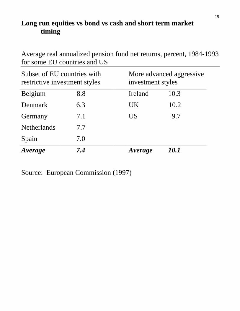
Long run equities vs bond vs cash and short term markettiming

Average real annualized pension fund net returns, percent, 1984-1993for some EU countries and US

Subset of EU countries withrestrictive investment styles

More advanced aggressiveinvestment styles

Belgium 8.8 Ireland 10.3

Denmark 6.3 UK 10.2

Germany 7.1 US 9.7

Netherlands 7.7

Spain 7.0

Average 7.4 Average 10.1

Source: European Commission (1997)

20

Hensel-Ziemba, 1942-1997, 56 years in Keim-Ziemba (2000)

A 100% US Small Caps Democrats

100% US Large Caps Republicans 14.1%/yr

B 60-40% Large Cap/Bonds 12.6%

A/B 24.5 times

• Studies such as Dimson, Marsh and Staunton (2000), Keim andZiemba (2000), Siegel (1998) and Goetzmann and Jorion (1999)have indicated that over long periods equity returns have greatlyoutperformed bond returns.

• Moreover, the longer the period the more likely is this dominanceto occur.

• How much to invest in cash, stocks and bonds over time is a deepand complex issue. For a theoretical analysis where theuncertainty of mean reversion is part of the model, see Barbaris(2000).

One thing is clear, equities have had an enormous advantage overcash and bonds during most past periods in most countries so that theoptimal blend is much more equity than 5%.

21

Between 1982 and 1999 the return of equities over bonds was over10% per year in EU countries.

• High equity returns of the distant past and the 1982-2000 bullmarket have led to valuations of price-earnings and other measuresthat in 1999-2001 were are at historically high levels in Europe,the US and elsewhere.

• Studies by Siegel (1999), Campbell and Shiller (1998), Berge andZiemba (2000) and especially Shiller (2000) suggest that thisoutperformance is unsustainable and the weak equity return resultsin 2000 and 2001 are consistent with this view.

The big questions is: will interest rate cuts in the US and othercountries lead to robust stock markets or will the poor returns last foryears?

• It is unclear when higher returns will return and whether they willbe very high in the 2001-2005 period.

• The specification of the benchmark (a linear combination of assets)around which the fund is to be evaluated greatly influences pensioninvestment behavior.

InnoALM is designed to help pension fund managers prudently makethese choices taking basically all aspects of the problem into account.

22

Austrian pension fund managers had considerably moreflexibility in their asset allocation decisions than the aboveinvestment rules would indicate.

• If an investment vehicle is more than 50% invested in bonds thanthat vehicle is considered to be a bond fund. Investment in 45%equities and 55% in bond funds (whose average bond and stockweightings are 60-40), gives a fund’s average equity of 67%,which is similar to that of the higher performing UK managers.

• Moreover, currency hedged assets are considered to be Eurodenominated.

• The minimum of 40% in Euro bonds is effectively a 40% limit onworldwide bonds but because of the above rules on weighting ofassets, this limit is not really binding either.

• The 5% rule on option premium means that managers hadeffectively full freedom for worldwide asset allocations.

• Use of the rules was not typical by actual pension fund managers.In some scenarios such allocations away from typical pension fundasset allocation in other Austrian pension funds could have led todisaster.

Without being armed with a model such as InnoALM whichcalculates the possible consequences of asset weight decisions, it wassafest for managers to go with the crowd.

23

Formulating the InnoALM as a multistage stochastic linearprogramming model

• Model determines the optimal purchases and sales for each of Nassets in each of T planning periods.

• Typical asset classes used at Innovest are US, Pacific, European,and Emerging Market equities and US, UK, Japanese andEuropean bonds.

• Objective is to maximize expected terminal wealth less convexpenalty costs subject to various constraints.

The stochastic program has a concave risk averse utility functionsubject to linear constraints.

• Decision variables are wealth (after transactions costs) itW ,purchases itP and sales itS for each asset (i=1,...,N).

• Purchases and sales take place at stages t=0,...,T–1.

• Returns are associated with time intervals. itR~ (t=1, ...,T) are the

(random) gross returns for asset i between t–1 and T. Tilda‘sdenote scenario-dependent random parameters or decisionvariables.

• Uncertainty is introduced by generating multiperiod scenariosusing statistical properties of the asset's returns.

• Optimal allocations are from a stochastic linear program using theIBMOSL library routines.

• Except for stage 0, purchases and sales are scenario dependent.

• Non-anticipatory constraints are imposed to guarantee that adecision made at a specific node is identical for all scenariosleaving that node. That is the future cannot be anticipated.

24

• Wealth accumulation

000 iiinit

ii SPWW −+= , t=0

110

~~~~iiiitit SPWRW −+= , t=1

itittiitit SPWRW~~~~~

1, −+= − , t=2,...,T-1

1,

~~~−= TiitiT WRW , t=T.

initiW is the prespecified initial value of asset i.

• Budget constraints are

01

01

0 )1()1( CtcsStcpP i

N

iii

N

ii +−=+ ��

==t=0,

ti

N

iiti

N

iit CtcsStcpP +−=+ ��

==

)1(~

)1(~

11

t=1,...,T–1,

itcp and itcs denote asset-specific linear transaction-costs forpurchases and sales, and tC is the fixed (non-random) net cashflow

• Short sales are not allowed, sales are no greater than currentholdings

initii WS ≤0 i=1,...,N t=0,

1,

~~~−≤ titit WRS i=1,...,N t=1,...,T–1.

25

• Model has built in bounds on portfolio weights so that the usermay specify the desired restrictions.

• Impact of such decisions may be investigated using the dual pricesobtained from the optimization of the large linear program inextensive.

• αk is the maximum percentage of asset k

0~~

1

≤− �=

N

iitkkt WW t=0,...,T-1.

• βk is the minimum percentage of asset k

0~~

1

≤+ �=

N

iitkkt WW t=0,...,T-1.

• Constraints on linear combinations of assets

0~~

1

≤−� � =lAi

N

iitAit WW ,

� � =

+−PBi

N

iitBit WW

1

~~ , t=0, …, T-1

where Al and Bp are the subsets of assets i=1, …, N

The αk’s, βk’s, γA’s, δB’s, Al ‘s and Bp’s may be time dependent.

26

In practice, Austrian, Germany and other European Union countrieshave specified restrictions that vary from country to country but notover time.

• Austrian limits:

a maximum of 40% in total equities

a maximum of 45% in foreign securities

a minimum of 40% in Euro currency bonds, and

a maximum 5% of total premiums in non-currency hedged optionshort and long positions.

• Typically, tW , the wealth target at stage t, is assumed to grow 7.5%in each period. This is a deterministic target goal for the increasein the pension fund’s assets assuming the number of employees inthe pension fund is in a steady state.

• Wealth targets

t=1,...,T,

where WtM

~ ≥0 is the wealth-target shortfall or slack variable.

27

• Benchmark targets tB~ are scenario dependent, based on stochastic

asset returns and on fixed weights defining the benchmarkportfolio.

�=

?+N

it

Btit BMW

1

~~~ t=1,...,T,

the variables BtM

~ equal the benchmark-target shortfalls.

• Shortfalls are also penalized by means of a piecewise linear convexrisk measure, which may differ from the penalty function forwealth targets.

• If total wealth is above the target a percentage , typically 0.1, ofthe exceeding amount is allocated to the reserve account. Thuswealth targets for future stages are further increased. For thatpurpose additional non-negative decision variables tD

~ areintroduced and the wealth target constraints above become

� �=

−

=−+=+−+−

N

i

t

jjtt

Wttititit DWMDSPW

1

1

1

~~~)

~~~( , t=1,...,T-1, where 0

~1 =D .

• Since actual pension payments are based on wealth levels,increasing these levels is tantamount to increasing pensionpayments.

• Deterministic target increases are typically targeted at 7.5% peryear.

• Actual reserves generated by the stochastic benchmark targetsprovide security for the pension plans increase of actual pensionpayments at each stage t.

28

• The pension plan’s concave risk averse objective function is tomaximize the expected present value of terminal wealth in period Tnet of expected penalty costs captured by the convex risk measure:

���

�

���

�√√↵

����

− ���

===

2

111

)~

(~

Max j

jtjj

T

ttt

N

iiTTS McvwdWdE ,

where )(?jc (j={W,B}) are the penalty functions for wealth- andbenchmark-targets.

• The jtu are weights attached to wealth- and benchmark target-shortfalls for each stage. jv are overall weights for the two types ofshortfalls.

• tw are overall weights for total shortfalls of each stage.

• Weights are normalized

121 =+ vv TvT

tt =�

=1

.

• tt rd −+= )1( , are discount factors and expectation is over T period

scenarios S.

• Usually the interest rate, r, is the three or six month Treasury-billrate. Campbell and Viceira (1998) argue that, in a multiperiodworld, the proper risk-free asset is an inflation-indexed annuityrather than the short dated T-bill. Analysis based on a model whereagents desire to hedge against unanticipated changes in the realrate of interest.

• Ten-year inflation-index bonds are then suggested for r as theirduration closely approximates the indexed annuity.

29

Liability side of the Siemens Pension Plan

• Employees, for which Siemens is contributing payments usingDCP

• Retired employees receiving pension payments.

• Simulation of the liabilities for a 30-year horizon assuming:

• Active employees are in steady state; staff replaced by a newemployee with the same qualification and sex.

• Salary is increasing 3.5 % to 4.5% annually.

• Annual Pension Plan contributions are a fixed fraction of salary

• The set of retired employees is modeled according to mortality andmarital tables

• Widows are entitled to 60% of the pension payments.

• Retired employees are receiving pension payments after reachingage 65 for men and 60 for women in accordance with the legalPension Plan.

• Pension payments to retired employees are calculated based uponthe individually accumulated contribution and performance duringactive employment; for the annuities a discount rate of 6% is used.

• Indexation of pension payments is set equal to 1.5% per annum tocompensate for inflation.

30

• Assets grow 7.5% per year to match liability growth.

• Liabilities related to active employees are simulated on anindividual level, due to the steady state assumption.

• Growth reflects only salary increases.

• Pensioners are likely to increase as currently active employees areretiring.

• Besides the target growth of assets, another output of thesimulation of liabilities is the estimated annual net cash flow ofplan contributions minus payments.

• Number of pensioners rising faster than plan payments.

• These cash flows are negative.

• Plan is declining in size.

Estimated payment growth breakdown active and retiredemployees, 2000-2030

0

50

100

150

200

250

300

350

400

20

00

20

02

20

04

20

06

20

08

20

10

20

12

20

14

20

16

20

18

20

20

20

22

20

24

20

26

20

28

20

30

Year

Paym

ents

(1999 =

100)

0

50

100

150

200

250

300

350

400

Pensioners

Active

Source: Innovest (2000)

31

Scenario Generation and Statistical Inputs

10 8 6 2

Scenario tree with a 10-8-6-2 node structure (960 total scenarios)

• Discrete scenarios

• Scenario dependent correlation matrices

• Fat tails/normal, t, general

• Means, standard deviations, correlations

• Embedded data1986-2000 bonds1970-2000 equity1992-2000 emerging market equity (also to 1800 for US and US)

• James-Stein mean reversion adjustments

32

Implementation, output and sample results

• An Excel spreadsheet is the user interface.

• The spreadsheet is used to select assets, define the number ofperiods and the scenario node-structure.

• The user specifies the wealth targets, cash in- and out-flows andthe asset weights that define the benchmark portfolio (if any).

• The input-file contains a sheet with historical data and sheets tospecify expected returns, standard deviations, correlation matricesand steering parameters.

33

Elements of InnoALM

Front-end user interface (Excel)• Periods (targets, node structure, fixed cash-flows, ...)• Assets (selection, initial values, transaction costs, ...• Liability data• Statistics (mean, standard deviation, correlation)• Bounds• Weights• Historical data• Options• Controls

GAUSS• read input• compute statistics• simulation returns (generate scenarios)• generate SMPS files

IBMOSL solver• read SMPS input files• solve the problem• generate output file (solutions for all nodes and variables)

Rear-end user interface (GAUSS)• read optimal solutions• generate tables and graphs• retain key variables in memory to allow for further analyses

34

Example

• Four asset classes (stocks Europe, stocks US, bonds Europe, andbonds US) with five periods (six stages).

• The periods are twice 1 year, twice 2 years and 4 years (10 yearsin total

• 10000 scenarios based on a 100-5-5-2-2 node structure.

• The wealth target grows at an annual rate of 7.5%.

• RA=4 and the discount factor equals 5.

• Theory: Kallberg-Ziemba (1983)

Means, standard deviations & correlations based on 1986-2000 data

StocksEurope

StocksUS

BondsEurope

BondsUS

Stocks US 0.763Bonds Europe 0.291 0.236Bonds US 0.493 0.763 0.286

normalperiods(70% of thetime) standard deviation 17.5 18.3 3.8 11.3

Stocks US 0.784Bonds Europe 0.178 0.107Bonds US 0.438 0.718 0.166

flat &decliningmarkets (20%of the time) standard deviation 18.3 21.1 4.1 12.2

Stocks US 0.832Bonds Europe -0.075 -0.182Bonds US 0.315 0.618 -0.104

crash periods(10% of thetime)

standard deviation 21.7 27.1 4.4 12.9all periods mean 12.0 13.0 6.5 7.2

35

N return distributions normally distributed and no mixing ofcorrelations matrices is performed

NM mixing correlations; 10% of the time, markets are extremelyvolatile, 20 % of the time there are flat or declining markets and70% of the time markets are assumed to be typically correlated.Mixing correlations also implies mixing different levels ofvolatility.

TM the same mixing proportions but equities have fat-tails. Annualreturns of all asset classes are well described by a joint normaldistribution. Monthly returns for equities are clearly non-normal. Equity returns have a t-distribution with 5 degrees offreedom.

TMCall assumptions of case TM but add Innovest's constraints onasset weights. Eurobonds must be at least 40% and equity atmost 40%.

36

Optimal initial asset weights at stage 0 obtained under variousassumptions

StocksEurope

StocksUS

BondsEurope

BondsUS

single-period, mean-varianceoptimal weights

15.6% 39.7% 44.7% 0.0%

case N: no mixing (only normalperiods);normal distributions

5.3% 48.1% 46.7% 0.0%

case NM: mixing correlations(70-20-10); normaldistributions

46.2% 49.6% 4.2% 0.0%

case TM: mixing correlations(70-20-10); t-distributions forstocks

56.1% 26.2% 17.7% 0.0%

case TMC: mixing correlations(70%-20%-10%); t-distributions for stocks;constraints on asset weights

27.7% 12.3% 60.0% 0.0%

Expected portfolio weights at the final stage in various cases.

StocksEurope

StocksUS

BondsEurope

BondsUS

case N 35.8% 53.5% 7.8% 3.0%

case NM 38.7% 51.8% 6.1% 3.3%

case TM 38.7% 53.3% 5.6% 2.4%

case TMC 17.7% 24.1% 46.2% 12.0%

37

• Break down the rebalancing decisions at later stages into groupsof achieved wealth level.

• This reveals the 'decision rule' implied by the model depending onthe current state.

• Quintiles of wealth were formed at stage 1 and the average optimalweights assigned to each quintile were computed.

Optimal weights conditional on the average level ofportfolio wealth at stage 1 and stage 4.

0%

20%

40%

60%

80%

100%

94.1 102.8 109.2 117.8 132.6

average wealth in quintile at stage 1

Bonds US

Bond Europe

Equities US

Equities Europe

0%

20%

40%

60%

80%

100%

143.1 174.3 205.3 243.5 333.7

average wealth in quintile at stage 4

Bonds US

Bond Europe

Equities US

Equities Europe

38

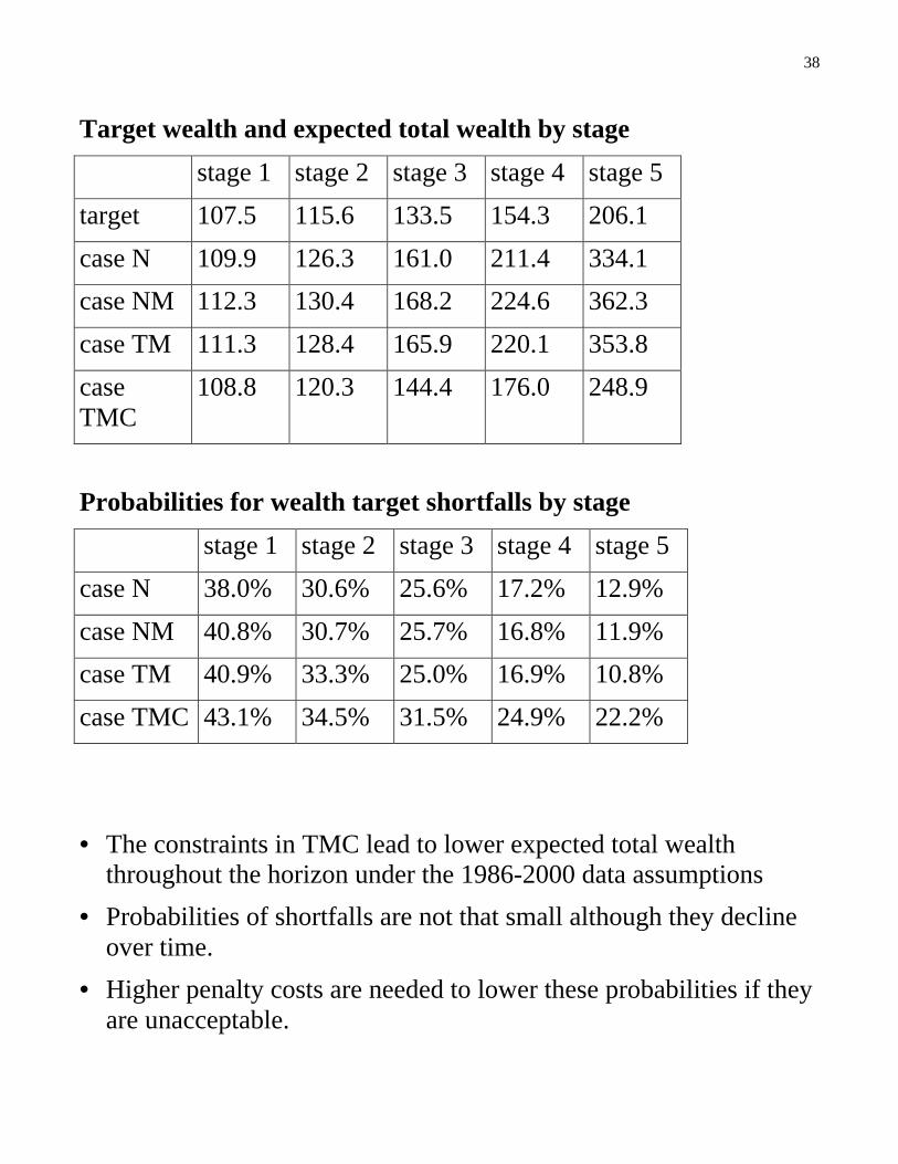
Target wealth and expected total wealth by stage

stage 1 stage 2 stage 3 stage 4 stage 5

target 107.5 115.6 133.5 154.3 206.1

case N 109.9 126.3 161.0 211.4 334.1

case NM 112.3 130.4 168.2 224.6 362.3

case TM 111.3 128.4 165.9 220.1 353.8

caseTMC

108.8 120.3 144.4 176.0 248.9

Probabilities for wealth target shortfalls by stage

stage 1 stage 2 stage 3 stage 4 stage 5

case N 38.0% 30.6% 25.6% 17.2% 12.9%

case NM 40.8% 30.7% 25.7% 16.8% 11.9%

case TM 40.9% 33.3% 25.0% 16.9% 10.8%

case TMC 43.1% 34.5% 31.5% 24.9% 22.2%

• The constraints in TMC lead to lower expected total wealththroughout the horizon under the 1986-2000 data assumptions

• Probabilities of shortfalls are not that small although they declineover time.

• Higher penalty costs are needed to lower these probabilities if theyare unacceptable.

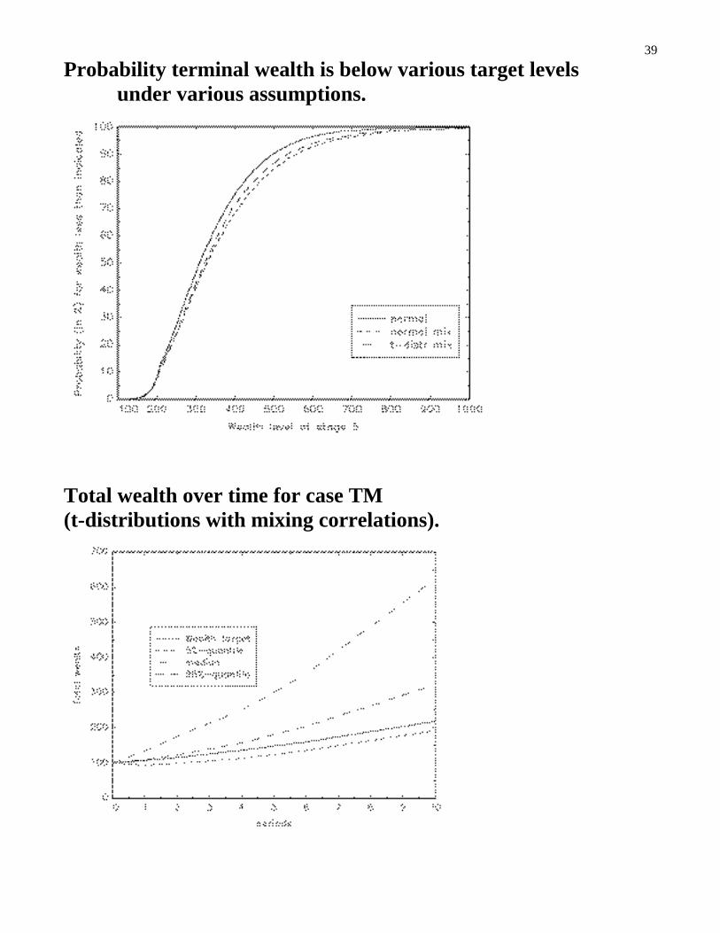
39

Probability terminal wealth is below various target levelsunder various assumptions.

Total wealth over time for case TM(t-distributions with mixing correlations).

40

• If the level of portfolio wealth exceeds the target, the surplus jD~

is allocated to a reserve account

• The expected value of reserves at stage t is computed from �=

t

jjD

1

~

• These values are in monetary units given an initial wealth level of100. They can be put into context by comparing them to the wealthtargets.

• For the unconstrained cases (N, NM and TM) expected reservescan go up to 130% of the target level at the final stage.

• Depending on the scenario the reserves can be as high as 2500.Their standard deviation (across scenarios) ranges from 10 at thefirst stage to 250 at the final stage.

Expected reserves by stage, w0=100

stage 1 stage 2 stage 3 stage 4 stage 5

case N 5 19 48 103 222

case NM 9 26 62 128 273

case TM 7 23 56 119 257

case TMC 4 10 23 45 87

41

Development of expected reserves across the planning horizon.

0

50

100

150

200

250

300

1 2 3 4 5 6 7 8 9 10

period (years)

normal

normal;mixing

t-distribution;mixing

t-distribution; mixingconstraints

Who is right? Abby Cohen/WTZ or Bob Shiller or ??

The effect associated with changing the forecasted future means ofequity returns.

• Econometric model shows that the future mean return for USequities is some value.

• The parameterized mean is assumed to be 6 to 16%.

• The mean of European equities is adjusted to maintain the relativemeans from the 1986-1990 data: the ratio of European and USequity means is 12/13.

• Retain all other assumptions of case TM (t-distribution and mixingcorrelations).

42

Optimal asset weights at stage 0 for varying levels of US equitymeans.

0%

20%

40%

60%

80%

100%

6 7 8 9 10 11 12 13 14 15 16

Mean return US equities

Bonds US

Bonds Europe

Equities US

Equities Europe

Probability for wealth target shortfall at all stages for varyinglevels of US equity means.

0

10

20

30

40

50

60

6 7 8 9 10 11 12 13 14 15 16

Mean return US equity

Pro

babi

lity

stage 1

stage 2

stage 3

stage 4

stage 5

43

The impact of the design of the scenario tree and the number ofstages.

• 10000 scenarios generated according to 100x20x5

• using periods of length one, three and six years (total ten years).

• same assumptions about returns statistics and consider case TM.

• A slightly more cautious policy is implemented if there are lessopportunities to rebalance the portfolio (19.3% versus 17.7%weight of bonds).

Comparing optimal portfolio weights at stage 0 and at the finalstage for a three-period and a five-period problem (10000scenarios each).

StocksEurope

StocksUS

BondsEurope

Bonds US

stage 03 periods

49.7% 31.0% 19.3% 0.0%

stage 05 periods

56.1% 26.2% 17.7% 0.0%

final stage3 periods

38.0% 58.6% 2.8% 0.6%

final stage5 periods

38.7% 53.3% 5.6% 2.4%

44

Conclusions and final remarks

• InnoALM is a tool to evaluate pension fund asset allocationdecisions.

• Multiple period scenarios/fat tails/uncertain means.

• Ability to make decision recommendations taking into accountgoals and constraints of the pension fund.

• Provides useful insight to pension fund allocation committee.

• Ability to see in advance the likely results of particular policychanges and asset return realizations.

• Gives more confidence to policy changes and recommends moreequity and less bonds than has traditionally been the case inAustria.