innovative statistical inference for anomaly detection in
TRANSCRIPT

Innovative Statistical Inference for Anomaly
Detection in Hyperspectral Imagery
by Dalton Rosario
ARL-TR-3339 September 2004 Approved for public release; distribution unlimited.
ARMY RESEARCH LABORATORY

NOTICES
Disclaimers The findings in this report are not to be construed as an official Department of the Army position unless so designated by other authorized documents. Citation of manufacturer’s or trade names does not constitute an official endorsement or approval of the use thereof. Destroy this report when it is no longer needed. Do not return it to the originator.

Army Research Laboratory Adelphi, MD 20783-1197
ARL-TR-3339 September 2004
Innovative Statistical Inference for Anomaly Detection in Hyperspectral Imagery
Dalton Rosario
Sensors and Electron Devices Directorate, ARL Approved for public release; distribution unlimited.

ii
REPORT DOCUMENTATION PAGE Form Approved
OMB No. 0704-0188 Public reporting burden for this collection of information is estimated to average 1 hour per response, including the time for reviewing instructions, searching existing data sources, gathering and maintaining the data needed, and completing and reviewing the collection information. Send comments regarding this burden estimate or any other aspect of this collection of information, including suggestions for reducing the burden, to Department of Defense, Washington Headquarters Services, Directorate for Information Operations and Reports (0704-0188), 1215 Jefferson Davis Highway, Suite 1204, Arlington, VA 22202-4302. Respondents should be aware that notwithstanding any other provision of law, no person shall be subject to any penalty for failing to comply with a collection of information if it does not display a currently valid OMB control number. PLEASE DO NOT RETURN YOUR FORM TO THE ABOVE ADDRESS.
1. REPORT DATE (DD-MM-YYYY)
September 2004 2. REPORT TYPE
Final 3. DATES COVERED (From - To)
October 2003 to September 2004 5a. CONTRACT NUMBER
5b. GRANT NUMBER
4. TITLE AND SUBTITLE
Innovative Statistical Inference for Anomaly Detection in Hyperspectral Imagery
5c. PROGRAM ELEMENT NUMBER
5d. PROJECT NUMBER
5e. TASK NUMBER
6. AUTHOR(S)
Dalton Rosario
5f. WORK UNIT NUMBER
7. PERFORMING ORGANIZATION NAME(S) AND ADDRESS(ES)
U.S. Army Research Laboratory ATTN: AMSRD-ARL-SE-SE 2800 Powder Mill Road Adelphi, MD 20783-1197
8. PERFORMING ORGANIZATION REPORT NUMBER ARL-TR-3339
10. SPONSOR/MONITOR'S ACRONYM(S)
9. SPONSORING/MONITORING AGENCY NAME(S) AND ADDRESS(ES)
U.S. Army Research Laboratory 2800 Powder Mill Road Adelphi, MD 20783-1197
11. SPONSOR/MONITOR'S REPORT NUMBER(S)
12. DISTRIBUTION/AVAILABILITY STATEMENT
Approved for public release; distribution unlimited.
13. SUPPLEMENTARY NOTES
14. ABSTRACT
A statistical motivated idea is proposed and its application to hyperspectral imagery is presented, as a viable alternative to testing a two-sample hypothesis using conventional methods. This idea led to the design of two novel algorithms for object detection. The first algorithm, referred to as semiparametric (SemiP), is based on some of the advances made on semiparametric inference. A logistic model, based on case-control data, and its maximum likelihood method are presented, along with the analysis of its asymptotic behavior. The second algorithm, referred to as an approximation to semiparametric (AsemiP), is based on fundamental theorems from large sample theory and is designed to approximate the performance properties of the SemiP algorithm. Both algorithms have a remarkable ability to accentuate local anomalies in a scene. The AsemiP algorithm is particularly more appealing, as it replaces complicated SemiP’s equations with simpler ones describing the same phenomenon. Experimental results using real hyperspectral data are presented to illustrate the effectiveness of both algorithms. 15. SUBJECT TERMS
Hyperspectral anomaly detection, large sample theory
16. SECURITY CLASSIFICATION OF: 19a. NAME OF RESPONSIBLE PERSON Dalton Rosaro
a. REPORT
Unclassified b. ABSTRACT
Unclassified c. THIS PAGE
Unclassified
17. LIMITATIONOF ABSTRACT
UL
18. NUMBER OF PAGES
40 19b. TELEPHONE NUMBER (Include area code)
(301) 394-4235 Standard Form 298 (Rev. 8/98) Prescribed by ANSI Std. Z39.18

iii
Content
List of Figures iv
Acknowledgment v
1. Introduction 1
1.1 Objective .........................................................................................................................1
1.2 Survey of Prior Art ..........................................................................................................1
2. Approach 3
2.1 Problem Formulation.......................................................................................................3
2.2 Statistical-Motivated Idea ...............................................................................................6
2.3 Logistic Model ................................................................................................................7
2.4 SemiP Algorithm.............................................................................................................9
2.5 Approximating SemiP Performance: AsemiP Algorithm .............................................10
3. Alternative Techniques 12
4. Results 13
4.1 Data Description............................................................................................................13
4.2 Implementation Notes ...................................................................................................14
4.3 Comparative Results .....................................................................................................15
5. Conclusion 19
6. References 20
Appendix A 23
Appendix B 27
Distribution List 31

iv
List of Figures
Figure 1. Nonhomogeneous, multicomponent scene from the hyperspectral digital imagery collection experiment (HYDICE). (A pixel in an HYDICE imagery is represented by a vector.) Typically, local anomaly detectors produce an intolerable high number of false alarms (non-anomalies) in similar scenes; local region discontinuities degrade detectors’ performances. The sampling mechanism is discussed in the text..............................................4
Figure 2. ROC curves for the HYDICE data scene shown in figure 1. The SemiP and AsemiP detectors are noticeably less sensitive to different decision thresholds; their performances almost achieve an ideal ROC curve for that scene, i.e., a step function starting at point (PFA=0,PD=1). ........................................................................................................................16
Figure 3. Decision surfaces for a HYDICE data scene (far left). The intensity of local peaks reflects the strength of evidences as seen by different anomaly detectors. Boundary issues were ignored in this test; surfaces were magnified to about the size of the original image only for the purpose of visual comparison...............................................................................17
Figure 4. Decision surfaces (3-dim version) produced by the SemiP and AsemiP detectors, their 2-dim versions are shown in figure 3. The dominant peaks represent the presence of the 14 targets parked near the treeline. Less-dominant peaks represent areas in the scene most prone to cause nuisance detections (e.g., region discontinuity). The SemiP and AsemiP detectors show a remarkable ability to accentuate genuine local anomalies from their surroundings. ...................................................................................................................18

v
Acknowledgment
I would like to take this opportunity to thank Prof. Rama Chellappa (UMD, U. of Md. at College Park), Prof. Benjamin Kedem (UMD), Prof. Eric Slud (UMD), and Dr. Nasser Nasrabadi (ARL) for occasional live discussions during the course of this work, and Dr. Patti Gillespie (ARL) for her encouragement and unconditional support.*
* This work was supported in pat by the ARL Director’s Research Initiative award FY04-SED-29.

vi
INTENTIONALLY LEFT BLANK

1
1. Introduction
1.1 Objective
This report focuses on the design of a new family of local anomaly detectors for hyperspectral sensor imagery (HSI). These detectors employ an indirect sample comparison via the mathematics of semiparametric statistics and large sample theory to test the likelihood that local HSI random samples belong to the same population, or class. The employed notion is not based on a physical motivation but on a statistical one, and it is proposed as a viable alternative to testing a two-sample hypothesis using conventional methods. The aim is to achieve a significant reduction of meaningless detections via unsupervised learning methods, while maintaining a high probability of meaningful detections. The notion I seek to implement is relatively simple, but some of the mathematics presented in this report are nontrivial, as Normality is not assumed in the models.
1.2 Survey of Prior Art
Hyperspectral sensors are passive sensors that simultaneously record images for many contiguous and narrowly spaced regions of the electromagnetic spectrum. A data cube is created from these images in which each image corresponds to the same ground scene and contains both spatial and spectral information about objects and backgrounds in the scene. These sensors employ several bands and have been used in various fields including urban planning, mapping, and military surveillance. Good references to some of these topics in the context of remote sensing and descriptions of the most popular sensors since the mid 1960’s are included in the reference section.1,2,3
With the introduction of sensors capable of high spatial and spectral resolution, there has been an increasing interest in using spectral imagery to detect objects or features of interest (targets). However, detection algorithms that presume a target signature are subject to signal mismatch losses because of the complications of converting sensor data into material spectra.4 Target matching approaches are further complicated by the large number of possible targets and uncertainty as to the reflectance/emission spectra of these objects. For example, the surface of a target may consist of several materials, and the spectra may be affected by weathering or other unknown factors. One may be interested in a large number of possible objects each with several signatures. Thus, the multiplicity of possible spectra associated with targets and complications of 1 Schowengerdt, 1997. 2 Coompbell, 1996. 3 Lillesand, 1994. 4 Schott, 1977.

2
atmospheric compensation have led to the development and application of anomaly detectors that seek to distinguish observations of unusual materials from typical background materials without reference to target signatures or target subspaces. Quite often objects consisting of unusual materials are detected as local anomalies in a scene; hence, anomaly detection will be used interchangeably in this paper with object detection.
Anomalies are defined with reference to a model of the background. Background models are developed adaptively using reference data from either a local neighborhood of the test pixel or a large section of the image. Local and global spectral anomalies are defined as observations that deviate in some way from the neighboring clutter background and from the overall scene, respectively. Both approaches have their merits. The local spectral anomaly detector is susceptible to false alarms that are isolated spectral anomalies. An algorithm commonly referred to as RX algorithm,5 for instance, has become a benchmark for multispectral data, based on this principle. The RX algorithm is a maximum likelihood anomaly detection procedure that simplifies the clutter to being spatially white. Researchers have also adapted some classic approaches6 (e.g., Fisher’s Linear Discriminant [FLD], Principal Component Analysis [PCA]) in the same spirit of the RX algorithm to anomaly detection in hyperspectral sensor imagery. Global spectral anomaly detection algorithms, on the other hand, are not susceptible to this type of clutter-generated false alarms. However, a global anomaly detector will not find an isolated target in the open if the signature is similar to that of previously classified background material. Examples of global detectors are the global normal mixture mode7 and the global linear mixture model.8 A comprehensive comparative analysis among different approaches for HSI anomaly detection can be found in.9,10,11,12
Earlier laboratory experiments using SAR (synthetic aperture radar) imagery13 produced compelling evidences to suggest that using conventional approaches to compare sample pairs, i.e., two-sample hypothesis tests treating the two samples individually, promotes an intolerable high number of meaningless detections (false alarms [FA]) in areas characterized by region discontinuities in the imagery. At that time, I proposed a post-processing method from mathematical morphology to account for those observations and adapted it to a SAR target-detection system.13,14 The approach produced some surprisingly good results using real SAR data. 5 Yu, 1997 6 Kwon, 2003. 7 Stein, 2002 8 Stein, 2002. 9 Manolakis, 2002. 10 Crist, 1999. 11 Haskett, 1999. 12 Grossmann, 1998. 13 Rosario, 1999. 14 Rosario, 2000.

3
The novelty in this paper is the mathematical means that is proposed to address HSI anomaly detection. The main contribution of this report is threefold: (i) a recently proposed local anomaly detector15 shall be discussed for the first time using extended details; I shall describe a suitable mathematical model16,17,18,19,20 that elegantly materializes a combining idea and shall study the model’s maximum likelihood method and its asymptotic behavior; I shall design an effective local anomaly detector based on the model’s asymptotic behavior, which for convenience shall be named the semiparametric (SemiP) algorithm; (ii) a second anomaly detector shall be proposed to the community, an approximation to the semiparametric (AsemiP) algorithm, which may be used to replace the complicated equations of the first model’s solution with simpler equations—yet describing the same phenomenon; I shall state a proposition of the second model and prove its statement. Derivation of the AsemiP algorithm is motivated by the SemiP’s output properties, not by the semiparametric model itself—although, its derivation is also based on approximation theorems of mathematical statistics; and (iii) in order to promote the use of models whose mathematics are based on the statistical assumption of independent, identically distributed random samples, an inside/outside window mechanism shall be introduced aimed at transforming local HSI information into independent sample pairs. Comparative results are also presented between SemiP, AsemiP and other approaches commonly used with hyperspectral data.
2. Approach
2.1 Problem Formulation
Figure 1 shows a hyperspectral scene that consists of 14 ground vehicles parked across a grassy area along a treeline. For surveillance applications in similar scenes, human analysts do well quickly ignoring most of the imagery and concentrating their attentions to those vehicles and their shadows. Humans, of course, use both global and local information to focus their attention to meaningful objects in the scene, a capability that can only be reproduced by applying, for instance, layers of unsupervised learning methods complementing each other to perform this single task. For example, a suite of algorithms that includes an edge detector, an edge elongation, a clustering method, and a morphological size test would probably reproduce the humans’ performance in such a scene, but with a huge cost: computational time.
15 Rosario, 2004 16 Qin, 1997. 17 Fokianos, 2001 18 Anderson, 1972. 19 Prentice, 1979. 20 Cox, 1996.

4
Figure 1. Nonhomogeneous, multicomponent scene from the hyperspectral digital imagery collection experiment (HYDICE). (A pixel in an HYDICE imagery is represented by a vector.) Typically, local anomaly detectors produce an intolerable high number of false alarms (non-anomalies) in similar scenes; local region discontinuities degrade detectors’ performances. The sampling mechanism is discussed in the text.
My interest is to approach humans’ performance using a single unsupervised learning algorithm that functions as a local anomaly detector. Figure 1 illustrates the sampling mechanism I propose to transform local imagery information into sample pairs for our statistical models. It introduces three window cells from which samples will be drawn from the data. These windows are referred to as: test cell, reference cell, and variability cell. Information between the variability and reference cells will be used to form a control or reference feature vector, and information between the variability and test cells will be used to form an unknown test feature vector.
The test cell provides a spectral sample average (µ1) from a (w x w) window; the reference cell provides a spectral sample average (µ0) from M vectors surrounding a guard region, i.e., a blind area between test and reference cells to account for larger than (w x w) targets; and the variability cell provides J individual spectral vectors (vj) each consisting of k = 1,…,K spectral
Scene Variability Cell Variability Cell
Reference Cell Test Cell
Vj^Aj^Äß-AjQ^
Visible/SWIR

5
responses (λjk) for K distinct wavelengths in the visible to SWIR (shortwave infrared) region of the electromagnetic spectrum, i.e., region from 0.4 µm to 2.4 µm.
Hyperspectral data have highly correlated—hence, dependent—spatial and spectral clutter, so to promote statistical independence, given that we will make this assumption in our models, I propose to apply a high-pass (HP) filter in the spectral domain, thus transforming vj into ∆j (see figure 1), and then use ∆j to compute a feature that promotes spatial independence. The feature is known as spectral angle mapper (SAM),21 which in essence computes the angle between two vectors, or
180 arccos ,tj i
j iijx µ
µπ
∆ ∆
∆ ∆
=
(1)
where ∆j = λjk - λj(k-1) (∆j is a [K-1] x 1 vector); ∆µi = λµi,k - λµi,(k-1) (using spectral components from vectors µ0 and µ1), xi = [xij]; i=0,1; j=1,…,J (J is the total number of vectors in the variability cell); xij range from 0 to 90 degrees (0 representing minimum class difference between reference and test samples and 90 representing the maximum class difference between these samples); the operator || z || denotes the squared root of ztz; and [*]t denotes the vector transpose operator.
Let x0 denote the reference feature vector, x1 the test feature vector, and let both vectors be distributed (~) by unknown joint distributions f0 and f1, respectively, or
)(~ ],,[
)(~ ],,[
00010
11111
0
1
xfxxx
xfxxx
n
n
=
= (2)
where, n0 = n1 = J in this particular implementation.
The window cells are expected to systematically move throughout the imagery and at each location this question will be posed: Do x0 and x1 belong to the same population, or class, in the feature space? If the answer is no, the test sample will be labeled as an anomaly with respect to its surroundings at that location.
A conventional two-sample hypothesis test would work very well if samples x0 and x1 do belong to distinct classes C0 and C1, or to one of these classes. Problems occur, however, when one of the samples (e.g., x0) belongs to a composite class consisting of both classes C0 and C1, denote x0(C0C1), and then it is compared to x1(C1). In those cases, standard statistical tests may reject the hypothesis that x0(C0C1) and x1(C1) belong to the same class. This rejection—correct as it may seem—is arguably the most dominant driving force affecting the number of FA produced by most—if not all—local anomaly detectors using sensor imagery. The reason is that region discontinuities (e.g., boundaries between tree clusters and their shadows) are abundant in sensor imagery, and they are not taken into account in conventional statistical models. 21 Kelly, April 1989.

6
2.2 Statistical-Motivated Idea
I propose an indirect comparison approach to circumvent the problem discussed in section 2.1. The approach is not based on a physical motivation but on a statistical one. The key is not to compare samples x0 and x1 directly, but to make that comparison indirectly by constructing a new sample z, consisting of both x0 and x1, and then by comparing z in some form to either x0 or x1. To clarify this notion, consider the following case studies when comparing x0 and x1: (1) samples belong to distinct classes, x0(C0) and x1(C1); (2) samples belong to a single class, x0(C0) and x1(C0); and (3) one of the samples holds information from two classes while the other sample belong to one of these classes, x0(C0C1) and x1(C1). Now consider the following, where U denotes the union of samples:
Case 1 Plausible Result
Conventional x0(C0) =? x1(C1) No
Proposed z(C0C1) = {x0(C0) U x1(C1)} =? x1(C1) No
Case 2 Plausible Result
Conventional x0(C0) =? x1(C0) Yes
Proposed z(C0C0) = {x0(C0) U x1(C0)} =? x1(C0) Yes
Case 3 Plausible Result
Conventional x0(C0C1) =? x1(C1) No
Proposed z(C0C1C1) = {x0(C0C1) U x1(C1)} =? x1(C1) Maybe
It is plausible that the proposed comparison approach would yield the same results produced by conventional methods for case studies 1 and 2, where No and Yes denote anomalies and non-anomalies, respectively. In particular, z in Case 1 would have been labeled as a strong anomaly in respect to x1 for the same reason a conventional test would have rejected the hypothesis that a composite sample (e.g., tree and shadow) belongs to the same class of a relatively pure sample (e.g., shadow). In Case 3, however, the proposed and conventional approaches would probably disagree in the intensity of their results because z(C0C1C1) shows more evidence of C1 than does

7
x0(C0C1). Sample x1(C1) would seem statistically closer to z(C0C1C1) than to x0(C0C1), and that difference would help to interpret x1(C1) as a soft-anomaly (labeled in Case 3 as Maybe).
My goal is to propose statistical models that are capable of accentuating, significantly, local anomalies (No) from soft-anomalies (Maybe) and non-anomalies (Yes). Such a capability would allow a detector to retain a high probability of correct detections while significantly reducing the number of nuisance detections. The first statistical model that I propose combines samples by relating in some form the probability distribution functions of x0 and x1. The model is discussed next.
2.3 Logistic Model
Let vectors xk have their components independently, identically distributed (iid). Let x0 be independent of x1. And consider the following:
1
0
1 11 1 1
0 01 0 0
[ , , ] ~ ( )
[ , , ] ~ ( ),n
n
x x x iid g x
x x x iid g x
=
= (3)
1
0
( ) exp( ( )),( )
g x h xg x
α β= + (4)
where g1 is regarded as an exponential distortion of g0 and h(x) is an arbitrary but known function of x. Note in (3)-(4) that no parametric assumption is given to g0 and that g1 depends only on the unknown parameters α and β, hence, justifying the model’s name: semiparametric.
The rationale for proposing to use (4), as our baseline, is that many common distribution families can be expressed as a canonical exponential function. These families fall under a category of probability density functions called exponential families, which are known to have many nice mathematical and statistical properties. (Some of these properties are discussed, for instance, in.22) One of these mathematical properties, for example, is that an exponential-family distribution can always be expressed as a shift of another exponential-family distribution, as shown in (4). Reference23 provides a good discussion on this topic.
Model (3)-(4) is based on case-control data and its mathematical development depends on some of the advances made on the theory of semiparametric inference. Semiparametric approaches are commonly used in analyzing binary data that arise in studying relationships between disease and
22 Casella, 1990. 23 Kay, 1987.

8
environment of genetic characteristics.18,19,20 Equation 4 has its roots in the standard logistic function having the general form
),()exp(1
)exp()( zz
zzP ηβγ
βγ≡
+++
= (5)
where γ is a scale parameter and β interpreted as a constant rate both defining a proportion P, which is dependent on a variable z. The logistic function was invented in the 19th century for the description of the growth of populations and the course of autocatalytic chemical reactions. Pierre-Francois Verhulst (1804-1849), a Belgian statistician, named5 as the logistic function and published his suggestions between 1838 and 1847. For an elaborate historical account, see.24
Using the independence assumptions in model (3)-(4), with h(x)= x, the MLE (maximum likelihood estimate) of α and β can be attained via the likelihood function,
. )exp()(
)()exp()(),,(
101
10
11
10
101
11
000
∏∏
∏∏
=
+=
=
==
+=
+=
n
jj
nnn
ii
j
n
jj
n
ii
xtg
xgxxgg
βα
βαβαζ (6)
where, n = n0+n1 and the combined feature vector t is
1 011 1 01 0 1[ , , , , , ] [ , , ].n n nt x x x x t t= = (7)
Notice in (6) that the part involving g0(ti) (reference distribution) reflects the combined-sample property of a model we sought, and the part involving the exponential distortion reflects only the property of the sample that is not the reference. Both properties fit well into the proposed framework of merging samples and then, in some form, comparing this combined structure with one of its original samples.
Notice also that g0 in (6) is unknown, thus, deriving MLE of α and β via standard procedures cannot be attained. However, using profiling one can express g0 in terms of α and β and then replace g0 with its new representation back in (6). Using profiling, the method of Lagrange multiplier was proposed18 to attain the maximization of ζ by fixing (α,β) and then maximizing ζ with respect to g0(ti) for i=1,…,n, subject to constraints
,0)(]1)[exp(
,0)(,1)(
0
00
=−+
≥=
∑∑
ii
ii
tgttgtg
βα (8)
5 Yu, 1997. 18 Anderson, 1972. 19 Prentice, 1979. 20 Cox, 1996. 24 Cramer, 2002.

9
where the last constraint reflects the fact that exp(α+βx)g0(x) is a distribution function. Following this approach, it can be shown16 that the maximum value of ζ is attained at
,
)exp(111)(
00
ii tn
tgβαρ ++
= (9)
where ρ=n1/n0, and that ignoring a constant, the log-likelihood function is
.])exp(1log[)(),(
111
1∑∑==
++−+=n
ii
n
ji txl βαρβαβα
(10)
A system of score equations that maximizes (10) over (α,β) is shown below,
0
]exp[1]exp[),(
11
=+++
+−=
∂∂
∑=
nt
tl n
i i
iβαρ
βαρα
βα (11)
.0
)exp(1)exp(),( 1
11=+
+++
−=∂
∂ ∑∑==
n
jj
n
i i
ii xt
ttlβαρ
βαρβ
βα (12)
Let (α∗,β∗) satisfy (11)-(12), then using (9) it can be shown16 that the MLE of g0(x) is
.
)exp(111)(ˆ **
00
ii
tntg
βαρ ++=
(13)
2.4 SemiP Algorithm
In this subsection, I adapt the theory in section 2.3 to the framework of object (anomaly) detection. The mathematics for this adaptation is nontrivial, as we employ the asymptotic behavior of (α∗,β∗) under a model that does not assume Normality. We strive to reach a reasonable balance between showing the most important parts of the mathematical development and length of this report.
First, notice that for g1(x) = exp(α + β x)g0(x) to be a density, a hypothesis of β = 0 in (4) must imply α = 0, as the term exp(α) functions as a normalizing factor so that g1 integrates over x to a total mass unity. Second, notice that the hypothesis H0: β = 0 (given that α must also be equal to zero) in (4) implies that a test population and a reference (control) population are equally distributed, namely, g1 = g0. With this logic, one can design an anomaly detector from the following composite hypothesis test:
0 1 0
1 1 0
: 0 ( ) anomaly absent : 0 ( ) anomaly present.
H g gH g g
ββ
= =
≠ ≠ (14)
16 Qin, 1997.

10
Under this test, local regions in the entire imagery would be individually tested to reject the null hypothesis (H0) yielding in the process a binary surface of values of 1, depicting a rejection of H0, and values of 0, depicting a non-rejection of H0. An isolated object in a scene would be expected to produce a cluster of 1 values (anomalies) in the resulting binary surface. But to design the hypothesis test in (14), one must know the asymptotic behavior of the extremum estimator β∗, which one can verify (see Appendix A) that it converges to Normality, or
1 2
* (1 )0, .( )
n NVar t
ρ ρβ− +
→
(15)
Squaring the left side of (15) and normalizing the result by the asymptotic variance, one can conclude (see convergence results, for instance, in22) that the resulting random variable
21
*2*2 )()1( χβρρχ →+= − tVn (16)
converges to a chi square distribution with 1 degree of freedom, where V*(t) estimates Var(t).
2.5 Approximating SemiP Performance: AsemiP Algorithm
In reference to (16), there are two major factors working in harmony and in complementary fashion to promote maximum separation between signal (anomalies) and noise (non-anomalies), they are: the squared value of β∗ and the estimated combined variance, V*(t), which is also quadratic.
These factors work in the following way: When two samples from the same class are compared (i.e., is H0: β=0 [g1=g0] true?), the term (β∗)2 tends to approach zero very fast, specially for β∗ values less than unity. On the other hand, if two samples from distinct classes are compared, the term V*(t) tends to a relatively high number, also very fast, asserting the fact that a combined sample vector t consists of components belonging to distinct populations.
Motivated by these properties, I shall state and prove an approximation algorithm based on large sample theory that replaces complicated SemiP equations with simpler ones describing the same phenomenon.
Proposition 1 (AsemiP Algorithm). Let
;)( , )( , ],,[
;)( , )( , ],,[200000010
211111111
0
1
∞<===
∞<===
σµ
σµ
iin
iin
xVarxEiidbexxx
xVarxEiidbexxx (17)
assume that x0 and x1 are independent and that, for some x0 and x1, the combined vector t
;)( , ],...,[],,,,,[ 21001111 0101
∞<=== += σtVariidis ttxxxxt nnnnn (18)
22 Casella, 1990.

11
and define
. , ;~
21
2
220
2
101σ
σζ
σ
σζµµβ ≡≡−≡
(19)
Under some regularity conditions, if hypothesis H0: ( )1 ;0~21 === ζζβ is true and
;1,0 , ,~̂
1
101 ==−= ∑
=
− ixnxxxin
kikiiβ
(20)
, , ,),()()(~
1
101
101
2 ∑∑=
−
==+=⋅−=
n
ii
n
ii tntwherennnxxgtttV
(21)
;11~ ;
)()(
)2(),(1
012
1
200
1
211
2
0101
−
==
+=
∑ −+∑ −
−=
nn and
xxxx
nxxgn
ii
n
ii
ρ
(22)
where, β̂ is an estimate of β , then the random variable
21
21 )(~~̂)1(~~ χβρχ →−= − tVn (23)
converges in distribution to a chi-squared distribution with 1 degree of freedom.
I shall make some insightful comments on (23) and refer the reader to its proof in Appendix B.
By inspection, one should readily recognize the behavior of the chosen function β~ , in Proposition 1, as it approximates the behavior of β. If two samples from the same population are compared using (23), the estimate of β~ , β̂~ in (20), would also tend to approach zero—as the sample size increases, and tend otherwise for samples belonging to distinct populations.
The real challenge, however, is to derive a relatively simple estimate of Var(t), as defined in (7A), to replace V*(t), as shown in (16). Var(t) is a sum of squared errors individually weighted by their probability of occurrence. In Proposition 1, g(x1,x0) is proposed to provide that probability feature, but as an average probability of occurrence, instead. In this sense, comparing two samples from distinct populations would produce very high cumulative square errors using the combined vector t, but appropriately weighted by an average proportion. The proof of Proposition 1 is presented in Appendix B.
In principle, the overall behavior of (23) seems to track that of (16), and both random variables are asymptotically identically distributed under 2
1χ . Note that the AsemiP’s performance will not asymptotically approach that of the SemiP’s performance, as the number of samples increases; the former approximates the general behavior of the latter, i.e., it promotes a high separation

12
between meaningful signals (isolated objects) from noise (homogeneous and non-homogenous local regions).
3. Alternative Techniques
In this section, I make a few general comments on four other anomaly detection techniques, which shall be used in this paper for comparison purposes: their mathematical representations are presented in this section, without proofs, and a reference that fully describes their implementation issues and performances in the HYDICE dataset will be cited.
The four techniques are known as: RX (reed-xiaoli), PCA (principal component analysis), EST (eigen separation transform), and FLD (Fisher’s linear discriminant). These techniques—or variations of them—are commonly used in the hyperspectral community. The RX technique is based on the generalized likelihood ratio test and on the assumption that the population distribution family of both test and reference samples are multivariate normal. The FLD technique is also based on the same assumption, but differs in its subtleties in answering the question whether the test and reference samples are drawn from the same normal distribution. The FLD technique promotes separation between classes and variance reduction within each class. The PCA and EST techniques are both based on the same general principle, i.e., data are projected from their original high dimensional space onto a significantly lower dimensional space using a criterion that promotes highest sample variability within each domain in this lower dimensional space. Differences between PCA and EST are better appreciated through their mathematical representations.
These four techniques were implemented with the conventional inside-outside window approach, where optimum window sizes were chosen to account for the target-size range of interest (see section 4.1), i.e., 5x5 inside window embraced by a 9x9 outside window and leaving a guard area between pixels 6 and 7, inclusive, from the center of the inside window. These techniques are represented by the following set of equations:
)()( 1outinout
toutinRX xxCxxScore −−= − (24)
)( outintinPCA xxEScore −= (25)
)( outint
CEST xxEScore −= ∆ (26)
)(/ outint
SSFLD xxEScorewb
−= (27)
where inx is a sample mean vector from the set of inside-window vectors, each having 150
spectral bands (see section 7.1); outx is similar but sampled from the outside window; 1outC− is

13
the inverse sample covariance using all vectors sampled from the outside window; tinE is the
highest energy eigenvector of the eigenvector decomposition of the inside-window covariance; tCE∆ is the highest positive energy eigenvector of the eigenvector decomposition of the
covariance difference (inside-widow minus outside-widow); and /b
tS SwE is the eigenvector
decomposition of the scatter matrices ratio 1B WS S − , where
∑∑==
−−+−−=M
i
tout
ioutout
iout
N
i
tin
iinin
iinW XxXxXxXxS
1
)()(
1
)()( ))(())(( (28)
∑∑==
−−+−−=M
i
ttotal
iouttotal
iout
N
i
ttotal
iintotal
iinB XxXxXxXxS
1
)()(
1
)()( ))(())(( (29)
and totalX is the total sample average using all samples from the inside and outside windows.
For additional details on the implementation and performance of these techniques, see.6
4. Results
4.1 Data Description
An experiment was carried out on the data set from the hyperspectral digital imagery collection experiment (HYDICE) sensor. The HYDICE sensor records 210 spectral bands in the visible to near infrared (VNIR) and short-wave infrared (SWIR) and, for the purpose of this paper, it is sufficient to know that each pixel in a scene is actually a vector, consisting of 210 components. An extended description of this dataset can be found, for example, in.25
The results shown in this section for one data sub-cube are representative for other sub-cubes in the HYDICE (forest radiance) dataset. An illustrative sub-cube (shown as an average of 150 bands; 640 x 100 pixels) is shown in figure 1 (left). (I only used 150 bands by discarding water absorption and low signal to noise ratio bands; the bands used are the 23rd-101st, 109th-136th, and 152nd-194th.) The scene consists of 14 stationary motor vehicles (targets near a treeline) in the presence of natural background clutter (e.g., trees, dirt roads, grasses). Each target consists of about 7x4 pixels, and each pixel corresponds to an area of about 1.3 x 1.3 square meters at the given altitude. The main goals of local anomaly detection algorithms on these types of scenes are to detect objects that seem clearly anomalous to its immediate surroundings, in some predetermined feature space, and to yield in the process a tolerable number of nuisance detections. Targets are often found to be anomalous to its immediate surroundings. 6 Kwon, 2003. 25 Schweizer, 2000.

14
4.2 Implementation Notes
I now present some helpful hints on the implementation of the SemiP and AsemiP algorithms.
1. SemiP Anomaly Detector
• Sampling Mechanism: Use the mechanism described in section 2.1 to sample a pair of random feature vectors xij (i = 0 [reference], 1 [test]; j=1,…,J) from HSI. I used a 9-pixel (3x3) test window, a 56-pixel reference window, and a 60-pixel variability window, as shown in figure 1. Note that the size of the variability window determines the size of the feature vectors, that is, x0j and x1j have the same size, J = 60.
• Statistical Independence: An attempt should be made to promote statistical independence in HSI. See discussion in section 2.1.
• Function Maximization: Perform an unconstrained maximization of l(α,β) in (10), or minimization of [-l(α,β)], to obtain the extremum estimates (α∗,β∗). For this report, I used one of the standard unconstrained minimization routines available in MATLABΤΜ software (i.e., fminsearch), and set the initial values of (α,β) to (0,0).
Variance Under the Null Hypothesis: V*(t) in (16) should be computed using (13) and a discrete version estimate of (7A):
)(ˆ)(ˆ)(;)(ˆ)(ˆ 122*0
== −== ∑ kki i
ki
k tEtEtVtgttE . (31)
• Decision Threshold: Using (16), high values of χ reject hypothesis Ho, hence, detecting anomalies. Set a decision threshold based on the Type I error, i.e., based on the probability of rejecting Ho given that Ho is true. Using a standard integral table for the chi square distribution, with 1 degree of freedom, find a threshold that yields an acceptable probability of error (e.g., 0.001), or alternatively find and use a suitable threshold that yields a value at the knee of the SemiP’s corresponding ROC curve.
2. AsemiP Anomaly Detector
In contrast to the SemiP algorithm, the AsemiP algorithm is significantly simpler to implement, as the latter suite does not require specialized subroutines (unconstrained minimization) to perform its function. Using the sampling mechanism described in section 2.1, the variables in Proposition 1 are straightforward to implement. One is also expected to promote statistical independence and to take a sufficiently large number of samples (larger than 30) to justify the use of approximation theorems of mathematical statistics. We used the sampling mechanism proposed in section 2.1 to obtain a pair of random feature vectors xij (i = 0 [reference], 1 [test]; j=1,…,J). I used a 9-pixel (3x3) test window, a 56-pixel reference window, and a 60-pixel variability window, as shown in figure 1, where J = 60. For a statistical decision, high values obtained by using (23), or equivalently (14B), reject the hypothesis Ho in Proposition 1, thus, detecting anomalies. Set a decision threshold based on a choice of type I error using, as the base

15
distribution, the chi-square distribution with 1 degree of freedom. Alternatively, find and use a suitable threshold that yields a value at the knee of the AsemiP’s corresponding ROC curve.
4.3 Comparative Results
ROC curves will be used in this subsection as a means to quantitatively compare the six approaches described in this paper.
As described in section 4.1, the set of 14 ground vehicles near the treeline in figure 1 constitutes our target set. However, since anomaly detectors are not designed to detect a particular target set, the meaning of false alarms is not absolutely clear in this context. For instance, a genuine local anomaly not belonging to the target set would be incorrectly labeled as a false alarm. Nevertheless, it does add some value to our analysis to compare detections of targets versus non-targets among the different algorithms.
Figure 2 shows ROC curves produced by the output of the six algorithms on the HYDICE data scene shown in figure 1. Detection performance was measured using the ground truth information for the HYDICE imagery. We used the coordinates of all the rectangular target regions and their shadows to represent the ground truth target set; call it TargetTruth. If we denote the region outside the TargetTruth as ClutterTruth, then the intersection between TargetTruth and ClutterTruth is zero and the entire scene is the union of TargetTruth and ClutterTruth. In this paper, for a given decision threshold, the proportion of target detection (PD) is measured as the proportion between the number of detected pixels belonging to TargetTruth over all pixels belonging to TargetTruth. On the other hand, the proportion of false alarms (PFA) is measured as the proportion between the number of detected pixels belonging to ClutterTruth over all pixels belonging to ClutterTruth.

16
Figure 2. ROC curves for the HYDICE data scene shown in figure 1. The SemiP and AsemiP detectors are noticeably less sensitive to different decision thresholds; their performances almost achieve an ideal ROC curve for that scene, i.e., a step function starting at point (PFA=0,PD=1).
In general, the quality of a detector can be readily assessed by noticing a key feature in the shape of its ROC curve: The closer the knee of a ROC curve is to the PD axis, the less sensitive the approach is to different decision thresholds. In other words, PFA does not change significantly as PD increases. (An ideal ROC curve resembles a step function that starts at point [PFA=0,PD=1].) As it can be readily assessed from figure 2, the SemiP and AsemiP detectors clearly outperform the other four techniques on the tested scene. That difference in performance can be better appreciated in figure 2 (right), where PFA is further restricted to a maximum value of 0.02 compared to 0.4 in figure 2 (left). Beyond the value of PFA = 0.4, these ROC curves reach PD near 1.0.
The significant display of performance shown in figure 2 by the proposed algorithms can be further appreciated by taking a closer look at the output surfaces produced by all six detectors, as they show evidences of local candidate anomalies in the scene. The intensity of local peaks shown in figure 3 reflects the strength of the evidence. It is evident from figure 3 that the surfaces produced by RX, PCA, EST, and FLD detectors are expected to be significantly more sensitive to changing decision thresholds then the ones produced by the SemiP and AsemiP detectors.
PI)
0(» 0 1 0 15 0? 0?1 0? 0 ?i
Proportion of False Alarms (PFA)
ScmiP TOCTWWPP A g 9 ft Qe^A+^
AsemiP
0 0.002 0.004 0.006 0.008 0.01 0.012 0.014 0.016 0.018 0.02
Proportion of False Alarms (PFA)

17
Although the 2-dim (2-dimensional) version of the output surfaces shown in figure 3 displays useful differences among the responses of the six detectors, they do not make full justice to the quality of the SemiP and AsemiP detectors, as a 3-dim perspective of their surfaces would. A 3-dim perspective of the SemiP’s and AsemiP’s output surfaces are depicted in figure 4.
Figure 3. Decision surfaces for a HYDICE data scene (far left). The intensity of local peaks reflects the strength of evidences as seen by different anomaly detectors. Boundary issues were ignored in this test; surfaces were magnified to about the size of the original image only for the purpose of visual comparison.
Both surfaces in figure 4 were clipped at the value of 3,000, but some of their values do continue to significantly higher numbers. The dominant (clipped) peaks are the results produced by the fourteen targets near the treeline.
Areas containing the presence of clutter mixtures (e.g., edge of terrain, edge of tree clusters), where other methods usually yield a high number of false alarms (false anomalies), are suppressed by the new approaches. The reason for this suppression is that, as part of the overall comparison strategy, the reference and test feature vectors are not compared as two individual samples. Instead, a new sample is constructed—the union of both cells—and compared to the test sample. This indirect comparison approach, which is inherent in both detectors, ensures that a component of a mixture (e.g., shadow) shall to be detected as a local anomaly when it is tested

18
Figure 4. Decision surfaces (3-dim version) produced by the SemiP and AsemiP detectors, their 2-dim versions are shown in figure 3. The dominant peaks represent the presence of the 14 targets parked near the treeline. Less-dominant peaks represent areas in the scene most prone to cause nuisance detections (e.g., region discontinuity). The SemiP and AsemiP detectors show a remarkable ability to accentuate genuine local anomalies from their surroundings.
against the mixture itself (e.g., trees and shadows). Performances of such cases are represented in figure 4 in the form of softer anomalies (significantly less-dominant peaks).
It is evident from figure 3 and figure 4 that both detectors perform remarkably well accentuating the presence of dominant local anomalies (e.g., targets and their shadows) from softer anomalies (e.g., region discontinuity). This ability explains the SemiP’s and AsemiP’s superior ROC-curve performances shown in figure 2.
Processing Time: For completeness, we report the processing time in minutes (min) for a cube of size 640 x 100 (pixels) x 150 (bands) using a personal computer (CPU speed: 1.80 GHz; RAM memory: 1.0 Gbytes), MATLAB software (release 13), and three detectors (RX, AsemiP, and SemiP). The recorded times were: 20.6 min (RX), 22.1 min (AsemiP), 42.9 min (SemiP). Computing the local variance-covariance matrix and its inverse dominated the RX processing time. Applying locally a HP filter in the spectral domain and applying SAM on the resulting vectors dominated the AsemiP processing time. And, finally, applying locally a HP filter and a
SemiP
3C0
0 0 o o

19
spatial SAM, and using an unconstrained minimization routine (see section 4.3) dominated the SemiP processing time.
5. Conclusion
I have presented an indirect approach to test two-sample hypotheses in HSI. The approach is not based on a physical motivation but on a statistical one. Using this approach, I designed two fully unsupervised object detectors (SemiP and AsemiP) for HSI. I showed performance agreement between these detectors through ROC curves, and other means. Performances of both detectors in the visible to short-wave infrared region of the spectrum were compared to performances of four other techniques. The proposed algorithms clearly outperform the others. The asymptotic distribution of the test statistic under Ho in both proposed algorithms is independent of the unknown parameters, which implies that both SemiP and AsemiP have the constant probability-of-error property. With this property, one can—in theory—select a decision threshold that yields a virtual zero probability of error. Error in this context means detection of non-anomalies, which is purely based on class similarities between test samples and their immediate surroundings, not necessarily non-targets (targets defined as particular objects of interest). This distinction should be noted.

20
6. References
1. Schowengerdt, R. A. Remote Sensing, Models and Methods for Image Processing, 2nd ed. Academic: San Diego, CA, 1997.
2. Campbell, J. B. Introduction to Remote Sensing, 2nd ed. Guilford: New York, 1996.
3. Lillesand, T. M.; Kiefer, R. W. Remote Sensing and Image Interpretation. Wiley: New York, 1994.
4. Schott, J. R. Remote Sensing: The Image Chain Approach. Oxford Univ. Press: Oxford, U.K., 1997.
5. Yu, X.; Hoff, L.; Reed, I.; Chen, A.; Stotts, L. Automatic target detection and recognition in multiband imagery: A unified ML detection and estimation approach, IEEE Tran. Image Processing, January 1997, 6, pp. 143–156.
6. Kwon, H.; Der, S.Z.; Nasrabadi, N.M. Adaptive anomaly detection using subspace separation for hyperspectral imagery. Opt. Eng. November 2003, 42 (11), pp. 3342–3351.
7. Stein, D. W.; Beaven, S. G. The fusion of quadratic detection statistics applied to hyperspectral imagery. IRIA-IRIS Proc. 2000 Meeting of the MSS Specialty Group on Camouflage, Concealment, and Deception, March 2002, pp. 271–280.
8. Stein, D.; Beaven, S.; Hoff, L.; Winter, E.; Scheaum, A.; Stocker, A. Anomaly detection from hyperspectral imagery. IEEE Signal Processing Mag, January 2002, 19, pp. 58–69.
9. Manolakis, D.; Shaw, G. Detection algorithms for hyperspectral imaging applications. IEEE Signal Processing Magazine January 2002, pp 29.
10. Crist, E., Schwartz, C.; Stocker, A. Pairwise adaptive linear matched-filter algorithm. in Proc DARPA Adaptive Spectral Reconnaissance Algorithm Workshop, January 1999.
11. Haskett, H. T.; Sood, A. K. Adaptive real-time endmember selection algorithm for sub-pixel target detection using hyperspectral data. in Proc. 1997 IRIS Specialty Group Camouflage, Concealment, Deception, October 1999.
12. Grossmann, J.; Bowles, J.; Hass, D.; Antoniades, J.; Grunes, M.; Palmadesso, P.; Gillis, D.; Tsang, K.; Baumback, M.; Daniel, M.; Fisher, J.; Triandaf, I. Hyperspectral analysis and target detection system for the adaptive-spectral reconnaissance program (ASRP). Proc SPIE, April 1998, 372, pp.2–13.

21
13. Rosario, D. S. Simultaneous Multi-Target Detection and False Alarm Mitigation Algorithm for the Predator UAV TESAR ATR System. Proc. of the 10th International Conference on Image Analysis and Processing (ICIAP'99), sponsored by the IEEE Computer Society, Venice, Italy, September 1999.
14. Rosario, D. S. End-to-End Performance of the TESAR ATR System. Proc. of the SPIE 14th Annual International Symposium on Aerospace/Defense Sensing, Simulation, and Control, Orlando, FL, April 2000.
15. Rosario, D. S. Highly Effective Logistic Regression Model for Signal (Anomaly) Detection. in Proc. 2004 IEEE ICASSP, Montreal, Canada, May 2004.
16. Qin , J.; Zhang, B. A goodness of fit test for logistic regression models based on case-control data. Biometrika, 1997, 84, 609–618.
17. Fokianos, K.; Kedem, B.; Qin, J. A semiparametric approach to the one-way layout. Technometrics 2001, pp. 56–65.
18. Anderson, J. A. “Separate sample logistic discrimination,” Biometrika 1972, 59, 19–35.
19. Prentice, R.; Pyke, R. Logistic disease incidence models and case-control studies. Biometrika 1979, 66, pp. 403–411.
20. Cox, D. R. Some procedures associated with the logistic qualitative response curve. Research Papers in Statistics: Festschrift for J. Neyman, John Wiley: New York, 1966, pp. 55–71.
21. Kelly, E. J. Adaptive Detection and Parameter Estimation for Multidimensional Signal Models, MIT Lincoln Laboratory: Lexington, MA, Tech. Rep. 848, April 1989.
22. Casella, G.; Berger, R. L. Statistical Inference, Duxbury Press: Belmont, CA 1990, pp. 112–120, 184, 222.
23. Kay, R.; Little, S. Transformations of the explanatory variables in the logistic regression model for binary data. Biometrika 1987, 74, 495–501.
24. Cramer, J. S. The Origin of Logistic Regression. Tinbergen Institute, U. of Amsterdam: TI 2002-119/4. Available on: http://ideas.repec.org/p/dgr/uvatin/20020119.html.
25. Schweizer, S. M.; Moura, J. M. F. Hyperspectral Imagery: Clutter Adaptation in Anomaly Detection. IEEE Trans. Information Theory August 2000, 46, no. 5, pp. 1855–1871.
26. Amemiya, T. Advanced Econometrics, Harvard U. Press : Cambridge, MA, 1985, pp. 110–112.

22
27. Lehmann, E. L. Theory of Point Estimation, Wadsworth & Brooks: Pacific Grove, CA, 1991, pp. 333–336, and Chapter 5.
28. Serfling, R. J. , Approximation Theorems of Mathematical Statistics, Wiley: New York, 1980, pp. 19.

23
Appendix A
Proof of the SemiP algorithm: Lemma 1A is relevant to estimators based on function maximization with respect to unknown parameters.
Lemma 1A.26 Assumptions:
(i) Let Θ be an open subset of the Euclidean K-space. (Thus the true value θo is an interior point of Θ.)
(ii) QT(y,θ) is a measurable function of vector y for all θ ∈Θ and /TQ θ∂ ∂ exists and is continuous in an open neighborhood N1(θo) of θo. (Note that this implies QT(y,θ) is continuous forθ ∈ N1, where T is the sample size.)
(iii) There exists an open neighborhood N2(θo) of θo such that T -1 QT(θ) converges to a nonstochastic function Q(θ) in probability uniformly in θ in N2(θo), and Q(θ) attains a strict local maximum at θo.
Let ΘΤ be set of roots of the equation
0=∂∂
θTQ (1A)
corresponding to the local maxima. If that set is empty, set ΘΤ equals to {0}. Then, for any ε >0,
.0])()(inf[lim 0
'0 =>−−
Θ∈∞→εθθθθ
θ TP
T
(2A)
In essence, Lemma 1A affirms that there is a consistent root of (1A). (For the proof, see26). Under certain conditions, a consistent root of (1A) is asymptotically Normal. The affirmation is shown in Theorem 1A, where asymptotic convergence is denoted by BA → .
Theorem 1A.26 Assumptions:
(i) All the assumptions of Lemma 1.
(ii) 2
'TQ
θ θ∂
∂ ∂ exists and is continuous in an open, convex neighborhood of θo.
(iii) 2
'TQ
θ θ∂
∂ ∂ converges to a finite nonsingular matrix
0
21
0 '( ) lim [ ( ) ]TQS E T θθθ θ
− ∂=
∂ ∂ in probability
for any sequence *Tθ such that *
0.Tθ θ=
26 Amemiya, 1985.

24
(iv) whereVNQT T )],(,0[)( 00
θθ θ →
∂∂ (3A)
].)()([lim)(
00 '1
0 θθθθ
θ∂
∂×
∂∂
= − TT QQTEV (4A)
Let ˆ{ }Tθ be a sequence obtained by choosing one element from ΘΤ defined in Lemma 1 such
that 0ˆ .Tθ θ→
Then ( ) ),,0(ˆ 0 whereNT T Σ→−θθ (5A)
1 10 0 0( ) ( ) ( ) .S V Sθ θ θ− −Σ = (6A)
For the proof, see also.26
The semiparametric model’s MLE solution satisfies the assumptions of Lemma 1A, including of course (1A) via (11) and (12). Therefore, by Lemma 1, (α∗,β∗) is consistent and, as we shall see by Theorem 1A, it converges asymptotically to a Normal distribution.
Under H0: β=0 (g1=g0), I shall use the following notation for the moments of t (the combined sample vector) with respect to the reference distribution g0:
)()()(
,)()(22
0
tEtEtVar
dttgttE kk
−≡
≡ ∫ (7A)
Let (α0,β0) be the true value of (α,β) under model (3)-(4) and assume ρ = n1/n0 remains constant
as both n1 and n0 go to infinity. Define ( ),α β∂ ∂
∂ ∂∇ ≡ and notice from (11) and (12) that
( )0 0, 0E l α β ∇ = . Under the null hypothesis (H0: β = 0 [g1 = g0]), using (4), (9), (11), (12)
and (7A) one can verify that
0 0
0 0
2exp( )0 0
1 01 exp( )
2 0 0 0 0
( , )1 ( )
( )[exp( ) ( )]
( ),1
t tt
l K g t dtn
K t g t t g t dt
E t
α βρ α β
α βα β
α β
ρρ
++ +
∂− →
∂ ∂
= ⋅ +
=+
∫
∫ (8A)
26 Amemiya, 1985.

25
where K1 and K2 are constants involving (n1,n0) and ρ/(1+ ρ) = n1/n (where n = n1+n0). Using similar argument to arrive at (8A) and applying the weak law of large numbers (WLLN) (see, for instance,27), one can use assumption (iii) in Theorem 1A to recognize that
+
=→∇∇−)()()(1
1),('1
200 tEtEtE
Sln ρ
ρβα (9A)
in probability as ∞→n . It follows that S is nonsingular and its inverse is
2
12 2
1 1( ) ( ) .( ) 1( ) ( )
E t E tSE tE t E t
ρρ
− +−= −− (10A)
Our interest is only in the parameter β, so, let Sβ denote the lower-right component of the expanded version of S –1 and use (7A) to obtain
.1
)(11
)()(1
22 ρρ
ρρ
β+
=+
−=
tVartEtES
(11A)
Using also the application of the central limiting theorem (CLT) in Theorem 1A (iv) and the fact that
[ ] ,0),( 00 =∇ βαlE (12A)
from (11) and (12), one can write
[ ]0 0 0 0( , ) [0, ( , )],n l N Vα β α β∇ → (13A)
where
[ ]0 0 1 2
1 ( ) 1( , ) 1 ( ).
( )( ) ( )
E tV E t
E tE t E tρρα β ρ+
= −
(14A)
V(α0,β0) is a direct result from (4A), see, for instance16. Using the conclusion of Theorem 1A, or (5A)-(6A), in terms of Sβ in (11A) and the lower-right component of the expanded version of V(α0,β0) in (14A), one can verify that
1 2
* (1 )0,( )
n NVar t
ρ ρβ− +
→
(15A)
16 Qin, 1997. 27 Lehmann, 1991.

26
and having the left side of (15A) normalized by the asymptotic variance and then squared, one can conclude (see convergence results, for instance, in22) that the resulting random variable
21
*2*2 )()1( χβρρχ →+= − tVn (16A)
converges to a chi square distribution with 1 degree of freedom, where V*(t) estimates Var(t). A multivariate solution is presented in17.
17 Fokianos, 2001. 22 Casella, 1990.
27
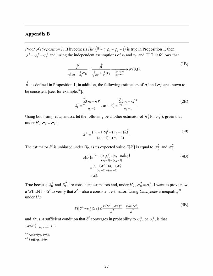
Appendix B
Proof of Proposition 1: If hypothesis H0: ( )1 ;0~21 === ζζβ is true in Proposition 1, then
20
21
2 σσσ == and, using the independent assumptions of x1 and x0, and CLT, it follows that
),1,0(
~̂~̂
10
11 11
01
01
01
Nnn
nnnn
→+
=+ ∞→
∞→σβ
σβ
(1B)
β̂ as defined in Proposition 1; in addition, the following estimators of 21σ and 2
0σ are known to be consistent [see, for example,26]:
( ) ( ).
1 and ,
1 0
1
200
20
1
1
211
21
01
−
∑ −=
−
∑ −= ==
n
xxS
n
xxS
n
ii
n
ii (2B)
Using both samples x1 and x0, let the following be another estimator of 20σ (or 2
1σ ), given that under H0 2
120 σσ = ,
.
)1()1()1()1(
01
200
2112
−+−−+−
=nn
SnSnS (3B)
The estimator S2 is unbiased under H0, as its expected value E[S2] is equal to 20σ and 2
1σ :
( ) ( ) ( )
.
)1()1()1()1(
)1()1()1()1(
20
01
200
211
01
200
2112
σ
σσ
=
−+−−+−
=
−+−−+−
=
nnnn
nnSEnSEn
SE (4B)
True because 20S and 2
1S are consistent estimators and, under H0 , 2 20 1σ σ= . I want to prove now
a WLLN for S2 to verify that S2 is also a consistent estimator. Using Chebychev’s inequality28 under H0:
2
2
2
220
220
2 )()()|(|εε
σεσ SVarSESP =
−≤≥−
(5B)
and, thus, a sufficient condition that S2 converges in probability to 20σ , or 2
1σ , is that ( ) ( ) 0
10 ,2 → ∞→nnSVar .
26 Amemiya, 1985. 28 Serfling, 1980.

28
Note that Var(S2) can be expressed as
[ ] [ ] )()()( 20
2
)1()1()1(2
12
)1()1()1(2
01
0
01
1 SVarSVarSVar nnn
nnn
−+−−
−+−− += (6B)
and, as 20S and 2
1S are both consistent estimators, their variances must converge to zero,
,0)( ;0)(01
20
21 → →
∞→∞→ nnSVarSVar (7B)
also
[ ] .1,0 ;0),(
2)1()1(
)1(0101
= → →∞−+−− knnnn
nk (8B)
Then ( )1 0
2,
( ) 0n n
Var S→∞
→ and, therefore, under H0:
.),( as ,1 102
21
2
20 ∞→→= nn
SSσσ (9B)
Using the same argument to arrive at (9B), we can also show that under H0:
,)( as ,1 012121
2
20
2
∞→+===→= nnnSS tt ζζσσ
(10B)
where 2tS is a consistent estimator of 2σ under H0, or
. ,)()1(1
1
1
212 ∑∑=
−
=
− =−−=n
ii
n
iit tntttnS (11B)
Furthermore, since 2tS is the sample variance of t (the combined vector) under H0, one can
readily verify that
∞→+=→= )( as ,1 01
10nnnSS tt
σσ (12B)
(see, for example,26 Chapter 5).
To finalize the proof, consider Theorem 1B below.
26 Amemiya, 1985.

29
Theorem 1B (Slutsky). Let Xn tend to X in distribution and Yn tend to c in probability, where c is a finite constant. Then
(i) Xn + Yn tend to X+c in distribution;
(ii) Xn Yn tend to cX in distribution;
(iii) Xn/Yn tend to X/c in distribution, if c is not zero.
See proof in.28
Using (1B), (9B), (12B) and the Slutsky Theorem, one can conclude that
)1,0(
~̂
10
10
2
20
01
01
NSS n
nt
nn
→
+ ∞→∞→σ
σσ
β (13B)
and that by squaring (13B) and using convergence results from,22 one can also conclude that
( ) ,~̂
~ 214
2
10
1
2
10
1
χβχ →+
=∞→∞→
nn
t
nn SS
(14B)
which can be readily reformatted into (23) using the definitions given in Proposition 1 and in this proof. Equation (14B) concludes the proof.
22 Casella, 1990. 28 Serfling, 1980.

30
INTENTIONALLY LEFT BLANK.

31
Distribution List
Admnstr Defns Techl Info Ctr ATTN DTIC-OCP (Electronic copy) 8725 John J Kingman Rd Ste 0944 FT Belvoir VA 22060-6218 DARPA ATTN IXO S Welby ATTN R Hummell 3701 N Fairfax Dr Arlington VA 22203-1714 Ofc of the Secy of Defns ATTN ODDRE (R&AT) The Pentagon Washington DC 20301-3080 Army Rsrch Physics Div ATTN AMSRD-ARL-RO-MM R Launer PO Box 12211 Research Triangle Park NC 27709-2211 AVCOM ATTN AMSAM-RD-WS-PL W Davenport Bldg 7804 Redstone Arsenal AL 35898 US Army TRADOC Battle Lab Integration & Techl Dirctrt ATTN ATCD-B 10 Whistler Lane FT Monroe VA 23651-5850 CECOM NVESD ATTN AMSRD-CER-NV-D J Ratches 10221 Burbeck Rd Ste 430 FT Belvoir VA 22060-5806 Dir for MANPRINT Ofc of the Deputy Chief of Staff for Prsnnl ATTN J Hiller The Pentagon Rm 2C733 Washington DC 20301-0300
US Army Aberdeen Test Center ATTN CSTE-DT-AT-WC-A Carlen ATTN CSTE-DTC-AT-TC-N D L Jennings 400 Colleran Road Aberdeen Proving Ground MD 21005-5059 US Army ARDEC ATTN AMSTA-AR-TD Bldg 1 Picatinny Arsenal NJ 07806-5000 US Army Aviation & Mis Lab ATTN AMSRD-AMR-SG-IP H F Anderson Redstone Arsenal AL 35809 US Army Avn & Mis Cmnd ATTN AMSAM-RD-SG-IP R Sims Redstone Arsenal AL 35898 Commanding General US Army Avn & Mis Cmnd ATTN AMSAM-RD W C McCorkle Redstone Arsenal AL 35898-5000 US Army CERDEC, NVESD ATTN AMSRD-CER-NV J Hilger ATTN AMSRD-CER-NV P Perconti ATTN AMSRD-CER-NV R Driggers FT Belvoir VA 22060-5806 US Army Natick RDEC Acting Techl Dir ATTN SBCN-TP P Brandler Kansas Street Bldg78 Natick MA 01760-5056 US Army PM NV/RSTA ATTN SFAE-IEW&S-NV D Ferrett 10221 Burbeck Rd FT Belvoir VA 22060-5806 US Army RDECOM ARDEC ATTN AMSRDL-AAR-QES P Willson Radiographic Laboratory, B.908 Picatinney Arsenal NJ 07806-5000

32
US Army Soldier & Biological Chem Ctr ATTN AMSSB-RRT-DP B Loerop Edgewood Chem & Biological Ctr Bldg E-5544 Aberdeen Proving Ground MD 21010-5424 US Army Tank-Automtv Cmnd RDEC ATTN AMSTA-TR-R G Gerhart Warren MI 48397-5000 US Army Topographic Engrg Ctr ATTN CEERD-RR-S R Rand 7701 Telegraph Rd Alexandria VA 22315 Commander USAISEC ATTN AMSEL-TD Blau Building 61801 FT Huachuca AZ 85613-5300 AFRL/SNAA ATTN M Jarratt 2241 avionics Circle Area B, Bldg 620 Wright Patterson AFB OH 45433-7321 CMTCO ATTN MAJ A Suzuki 1030 S Highway A1A Patrick AFB FL 23925-3002 SMDC ATTN SMDC-TC-TD-YF A Aberle PO Box 1500 Redstone Arsenal AL 35898
SITAC ATTN H Stiles ATTN K White ATTN R Downie 11981 Lee Jackson Memorial Hwy Suite 500 Fairfax VA 22033-3309 Director US Army Rsrch Lab ATTN AMSRD-ARL-RO-D JCI Chang ATTN AMSRD-ARL-RO-EL W Sander PO Box 12211 Research Triangle Park NC 27709-2211 US Army Rsrch Office ATTN AMSRD-ARL-RO-PP R Hammond PO box 12211 Research Triangle Park NC US Army Rsrch Lab ATTN AMSRD-ARL-CI-OK-T Techl Pub (2 copies) ATTN AMSRD-ARL-CI-OK-TL Techl Lib (2 copies) ATTN AMSRD-ARL-D A Grum ATTN AMSRD-ARL-D J M Miller ATTN AMSRD-ARL-SE J Pellegrino ATTN AMSRD-ARL-SE J Rocchio ATTN AMSRD-ARL-SE-S J Eicke ATTN AMSRD-ARL-SE-SE D Rosario (5 copies) ATTN AMSRL-SE-SE N Nasrabadi ATTN AMSRL-SE-SE P Gillespie ATTN IMNE-AD-IM-DR Mail & Records Mgmt Adelphi MD 20783-1197