ISO-NE PUBLIC

M A Y 1 5 , 2 0 1 9 | T E L E C O N F E R E N C E

Resource Studies and AssessmentsP E T E R W O N G A N D F E I Z E N G

Installed Capacity Requirement Development Webinar

ISO-NE PUBLIC

Disclaimer

2

ISO New England (ISO) provides information sessions to enhance participant and

stakeholder understanding. Not all issues and requirements are addressed by the technical

session. Consult the effective Transmission, Markets and Services Tariff and the relevant

Market Manuals, Operating Procedures and Planning Procedures for detailed information.

In case of a discrepancy between the technical session provided by ISO and the Tariff or

Procedures, the meaning of the Tariff and Procedures shall govern.

ISO-NE PUBLIC

Purpose

3

Explain how Installed Capacity Requirement (ICR) and other associated values used in the Forward Capacity Market (FCM) are developed

ISO-NE PUBLIC

Topics

• ICR Background

• ICR Calculations

• Simulation Model for Resource Adequacy Reliability Assessments

• System and Locational Capacity Requirements

• FCM System and Zonal Demand Curves

• ICR Assumption Developments

• Tie Benefits

• Summary

4

ISO-NE PUBLIC

Installed Capacity Requirement Background

5

ISO-NE PUBLIC

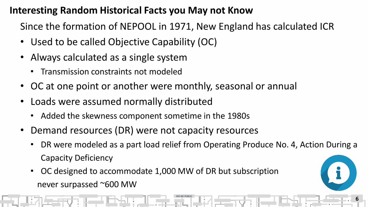
Interesting Random Historical Facts you May not Know

Since the formation of NEPOOL in 1971, New England has calculated ICR

• Used to be called Objective Capability (OC)

• Always calculated as a single system

• Transmission constraints not modeled

• OC at one point or another were monthly, seasonal or annual

• Loads were assumed normally distributed

• Added the skewness component sometime in the 1980s

• Demand resources (DR) were not capacity resources

• DR were modeled as a part load relief from Operating Produce No. 4, Action During a

Capacity Deficiency

• OC designed to accommodate 1,000 MW of DR but subscription

never surpassed ~600 MW

6

ISO-NE PUBLIC

Interesting Random Historical Facts you May not Know, cont.

• Capacity imports had priority over tie benefits

• Limited by transmission line import capability

• Tie benefits based on left over import capability

• OP-4 load relief were not used to meet ICR

• OP-4 load relief assumption used to include load relief from customer

appeals

• Tie benefits were seasonal – summer and winter

• Reflect the value of the Firm Energy Contract with hydro Quebec over the Phase II tie

• ICR would change based on the performance of new units

• Credits for units that decrease ICR

• Penalties for units that increase ICR

7

ISO-NE PUBLIC

8

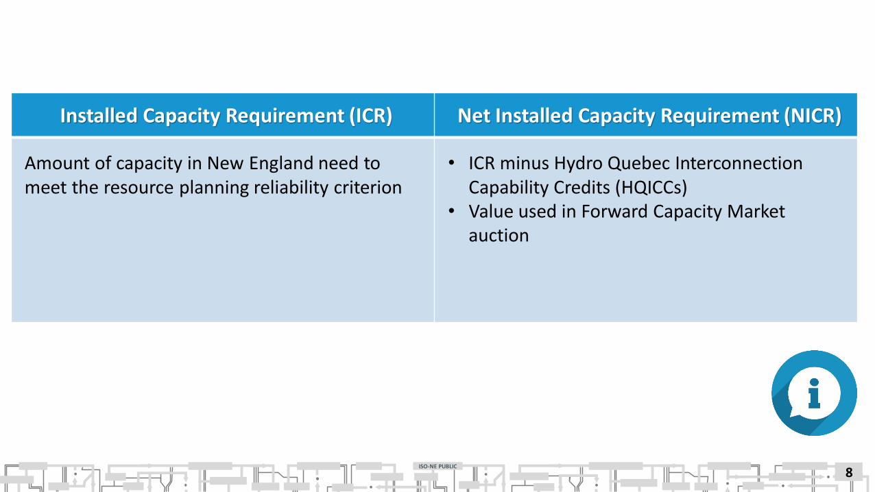
Installed Capacity Requirement (ICR) Net Installed Capacity Requirement (NICR)

Amount of capacity in New England need to meet the resource planning reliability criterion

• ICR minus Hydro Quebec Interconnection Capability Credits (HQICCs)

• Value used in Forward Capacity Market auction

ISO-NE PUBLIC

Installed Capacity Requirement Needed to Meet Compliance

ISO is required to conduct ICR calculations to meet compliance requirements

• Section III.12 of ISO Market Rule 1 – Calculation of Capacity Requirements

‒ Develop Installed Capacity Requirement (ICR)-Related Values for each FCM auction:

FCA, ARA1, ARA2, and ARA3

‒ Use a stakeholder process (NEPOOL committee processes) to develop ICR-Related Values

‒ File values with FERC for approval

• Northeast Power Coordinating Council (NPCC) Regional Reliability Reference Directory # 1 –

Design and Operation of Bulk Power System requires ISO New England to do the following:

‒ Conduct comprehensive review of resource adequacy every three years with an interim

update for years in between

‒ Demonstrate to NPCC that New England system meets the resource adequacy design criterion

9

ISO-NE PUBLIC

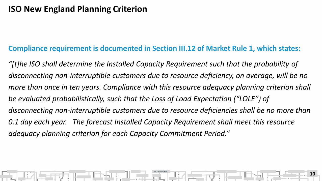
ISO New England Planning Criterion

Compliance requirement is documented in Section III.12 of Market Rule 1, which states:

“[t]he ISO shall determine the Installed Capacity Requirement such that the probability of

disconnecting non-interruptible customers due to resource deficiency, on average, will be no

more than once in ten years. Compliance with this resource adequacy planning criterion shall

be evaluated probabilistically, such that the Loss of Load Expectation (“LOLE”) of

disconnecting non-interruptible customers due to resource deficiencies shall be no more than

0.1 day each year. The forecast Installed Capacity Requirement shall meet this resource

adequacy planning criterion for each Capacity Commitment Period.”

10

ISO-NE PUBLIC

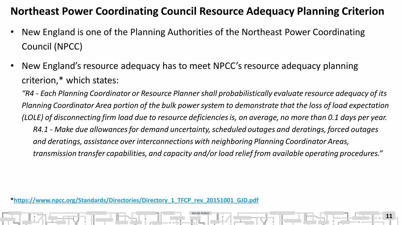
Northeast Power Coordinating Council Resource Adequacy Planning Criterion

• New England is one of the Planning Authorities of the Northeast Power Coordinating

Council (NPCC)

• New England’s resource adequacy has to meet NPCC’s resource adequacy planning

criterion,* which states:

“R4 - Each Planning Coordinator or Resource Planner shall probabilistically evaluate resource adequacy of its

Planning Coordinator Area portion of the bulk power system to demonstrate that the loss of load expectation

(LOLE) of disconnecting firm load due to resource deficiencies is, on average, no more than 0.1 days per year.

R4.1 - Make due allowances for demand uncertainty, scheduled outages and deratings, forced outages

and deratings, assistance over interconnections with neighboring Planning Coordinator Areas,

transmission transfer capabilities, and capacity and/or load relief from available operating procedures.”

*https://www.npcc.org/Standards/Directories/Directory_1_TFCP_rev_20151001_GJD.pdf

11

ISO-NE PUBLIC

Shows market participants expected capacity

needs of region

• FCM Period (Years 1-3) - Actual ICRs are the latest

values approved by FERC for the FCM auctions

• Beyond FCM timeframe - Representative ICRs are

values calculated to inform market participants of

region’s needs

Installed Capacity Requirement Needed to Meet Resource AdequacyAssessments

12

Results of up to 10 years of ICR calculations are used in:

Regional System Plan (RSP)

ISO-NE PUBLIC

Installed Capacity Requirement Development Process Timeline for FCM

13

ISO develops necessary assumptions, according to

Section III.12 of Market Rule 1, and reviews them

with PSPC

(May – August)

ISO calculates ICR-Related Values and

reviews them with PSPC (August – October)

After PSPC reviews and comments, ISO may

recalculate ICR-Related Values (August – October)

Presents PSPC recommended

ICR-Related Values and assumptions to Reliability

Committee (RC) for comment

(August – September)

RC takes action on the PSPC recommended FCA

ICR-Related Values(September)

Annual process involving stakeholders normally runs from April through December and consists of the following:

RC takes action on the PSPC recommended ARAs

ICR-Related Values(October)

ICR-Related Values for three ARAs to be conducted in following year filed with FERC

(December 1 for ARAs)

Participants Committee (PC) takes action on the

PSPC recommended FCAICR-Related Values

(October)

PC takes action on the PSPC recommended ARAs

ICR-Related Values(November)

ICR-Related Values for FCA filed with FERC

(Early November)

ISO-NE PUBLIC

Installed Capacity Requirement Development Process Timeline forRSP, NPCC, and NERC Assessments

14

Actual and representative ICR values are developed in around

May of Regional System Plan (RSP) publication year

ISO reviews with Planning Advisory Committee

New England resource needs for Northeast Power Coordinating

Council (NPCC) Resource Adequacy Review are developed in

September

ISO reviews with NPCC CP 8 Working Group, NPCC Task Force on Coordination of Planning andReliability Coordinating Committee

ISO-NE PUBLIC 15

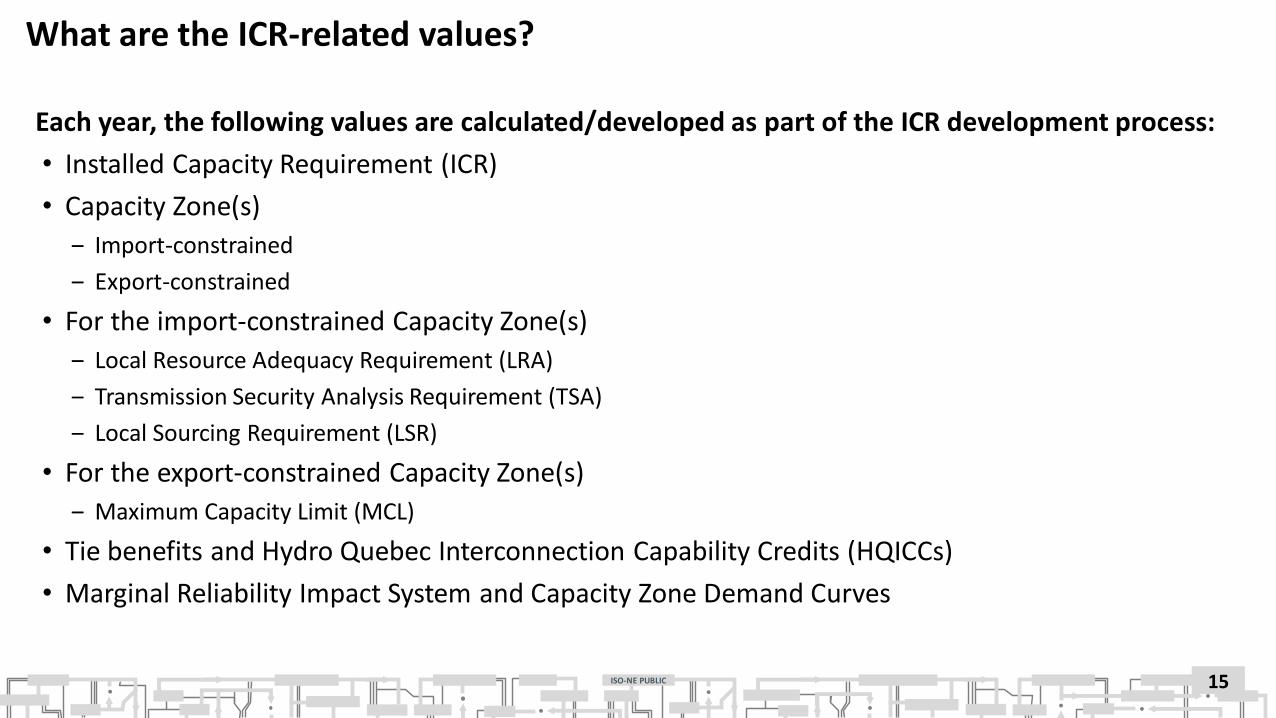
What are the ICR-related values?

Each year, the following values are calculated/developed as part of the ICR development process:

• Installed Capacity Requirement (ICR)

• Capacity Zone(s)

‒ Import-constrained

‒ Export-constrained

• For the import-constrained Capacity Zone(s)

‒ Local Resource Adequacy Requirement (LRA)

‒ Transmission Security Analysis Requirement (TSA)

‒ Local Sourcing Requirement (LSR)

• For the export-constrained Capacity Zone(s)

‒ Maximum Capacity Limit (MCL)

• Tie benefits and Hydro Quebec Interconnection Capability Credits (HQICCs)

• Marginal Reliability Impact System and Capacity Zone Demand Curves

ISO-NE PUBLIC

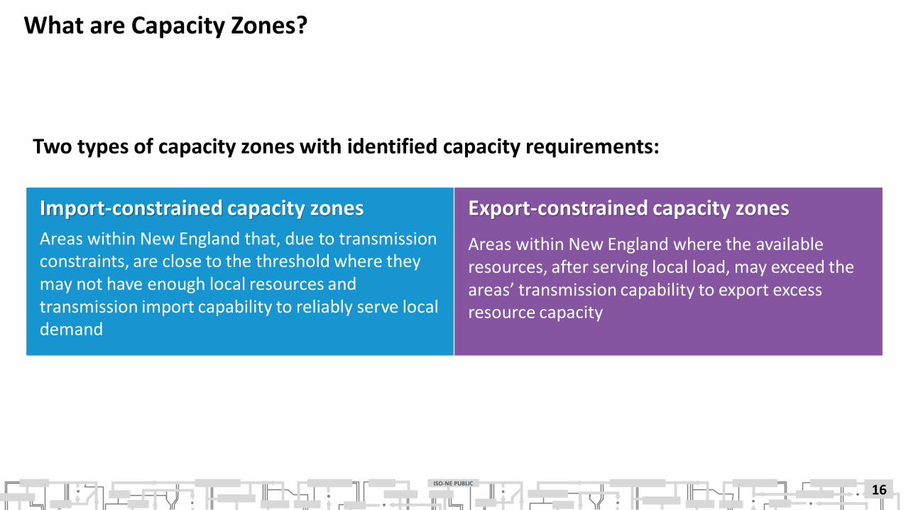
What are Capacity Zones?

Two types of capacity zones with identified capacity requirements:

16

Import-constrained capacity zones

Areas within New England that, due to transmission constraints, are close to the threshold where they may not have enough local resources and transmission import capability to reliably serve local demand

Export-constrained capacity zones

Areas within New England where the available resources, after serving local load, may exceed the areas’ transmission capability to export excess resource capacity

ISO-NE PUBLIC

17

Local Resource Adequacy Requirement (LRA)

Minimum amount of resources, determined probabilistically, that must be located in a zone to meet system-reliability requirement

Transmission Security Assessment Requirement (TSA)

• Deterministic reliability screen of an import-constrained area

• Basic security review to determine requirement of import-constrained area to meet its load through internal generation and import capability

Local Sourcing Requirement (LSR)

Minimum amount of capacity that must be electrically located within an import-constrained capacity zone

• Value representing point where adding more capacity in an import-constrained zone may no longer improve system

reliability more than adding capacity elsewhere in system

• Mechanism used to assist in valuing capacity appropriately in constrained areas

• Amount of capacity needed to satisfy the higher of LRA or TSA

Higher of the Two

ISO-NE PUBLIC

What is Maximum Capacity Limit?

Maximum amount of capacity that is

electrically located in an export-constrained

capacity zone used to meet the Installed

Capacity Requirement

• Value representing point where adding more

capacity in an export-constrained zone may no

longer improve system reliability as much as

adding capacity elsewhere in the system

18

ISO-NE PUBLIC

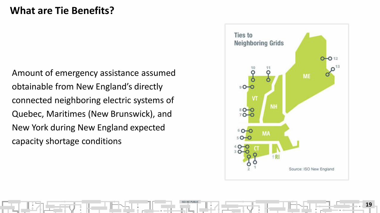
What are Tie Benefits?

Amount of emergency assistance assumed

obtainable from New England’s directly

connected neighboring electric systems of

Quebec, Maritimes (New Brunswick), and

New York during New England expected

capacity shortage conditions

19

ISO-NE PUBLIC

What are Hydro Quebec Interconnection Capability Credits?

• Tie benefits associated with Hydro Quebec Phase I/II HVDC Transmission Facilities

(HQ Phase II)

• Capacity credits that are allocated to Interconnection Rights Holders, which are entities

that pay for and, consequently, hold certain rights over the HQ Phase II interconnection,

in proportion to their individual rights over the HQ Phase II interconnection

• ISO must file Hydro Quebec Interconnection Capability Credits (HQICCs) values with

FERC for FCM

20

ISO-NE PUBLIC

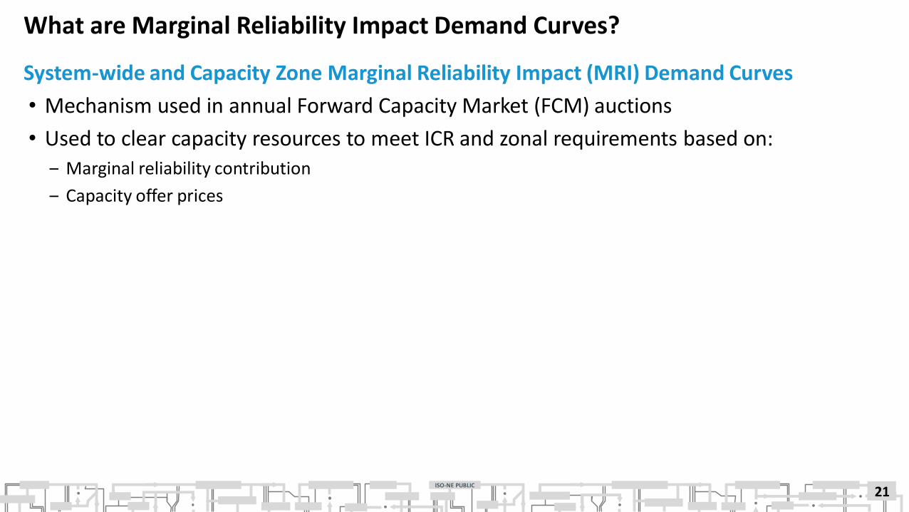
What are Marginal Reliability Impact Demand Curves?

System-wide and Capacity Zone Marginal Reliability Impact (MRI) Demand Curves

• Mechanism used in annual Forward Capacity Market (FCM) auctions

• Used to clear capacity resources to meet ICR and zonal requirements based on:

‒ Marginal reliability contribution

‒ Capacity offer prices

21

ISO-NE PUBLIC

Installed Capacity Requirement Calculations

22

ISO-NE PUBLIC

Installed Capacity Requirement Calculations

Based on probabilistic analysis to measure the risks of insufficient resources to serve load

• Reliability indices that quantify risks are a part of simulation model output

•

23

Loss of Load Expectation (LOLE)Expected days of system not having

enough capacity to serve load

Loss of Load Hours (LOLH)Expected hours of system not having

enough capacity to serve load

Expected Energy Not Served (EENS)Expected amount of energy from loss of

load events

Used for determining ICR values Used in developing the demand curves

ISO-NE PUBLIC

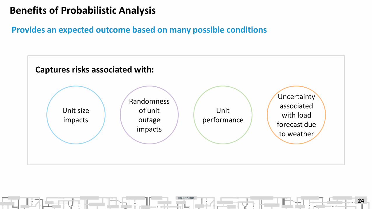
Benefits of Probabilistic Analysis

Provides an expected outcome based on many possible conditions

24

Unit size impacts

Randomness of unit outage impacts

Unit performance

Uncertainty associated with load

forecast due to weather

Captures risks associated with:

ISO-NE PUBLIC

Risk Factors Considered in Installed Capacity Requirement Calculations

• Resource availability due to planned and unplanned outages

‒ Risks from resource unplanned outages are considered random and independent; one resource outage does not

affect outage of another resource

‒ Resource annual maintenance requirement is an input to represent planned outage (MARS would distribute resource

Maintenance to the weeks with the lowest risk of load loss)

• Deliverability of resources due to transmission limitation

• Load forecast uncertainty (due to weather)

25

Examples of correlated risks:• All areas/regions see the same heat wave at the same time• Resource outage can be correlated to an interface rating change• Seasonal derating affecting similar generator

Operational risks are not considered (perfect foresight)• All resources are assumed to be available if they are not on outage• All resources are assumed to be committed in a timely manner• No resources are unavailable due to higher than expected loads

ISO-NE PUBLIC

Simulation Model for Resource Adequacy Reliability Assessments

26

ISO-NE PUBLIC

General Electric Multi-Area Reliability Simulation Model (MARS)

• Computer program that uses a sequential Monte Carlo simulation to probabilistically

compute the resource adequacy of the system by simulating the random nature of

resources and the uncertainty of load forecast

• Major transmission interfaces are modeled by using the pipe and bubble approach

(subarea presentation with limitations between subareas)

between subareas ‒ Loads and generators are assumed to be connected to different subareas within the system

27

Rest of Pool

Maine

ISO-NE PUBLIC

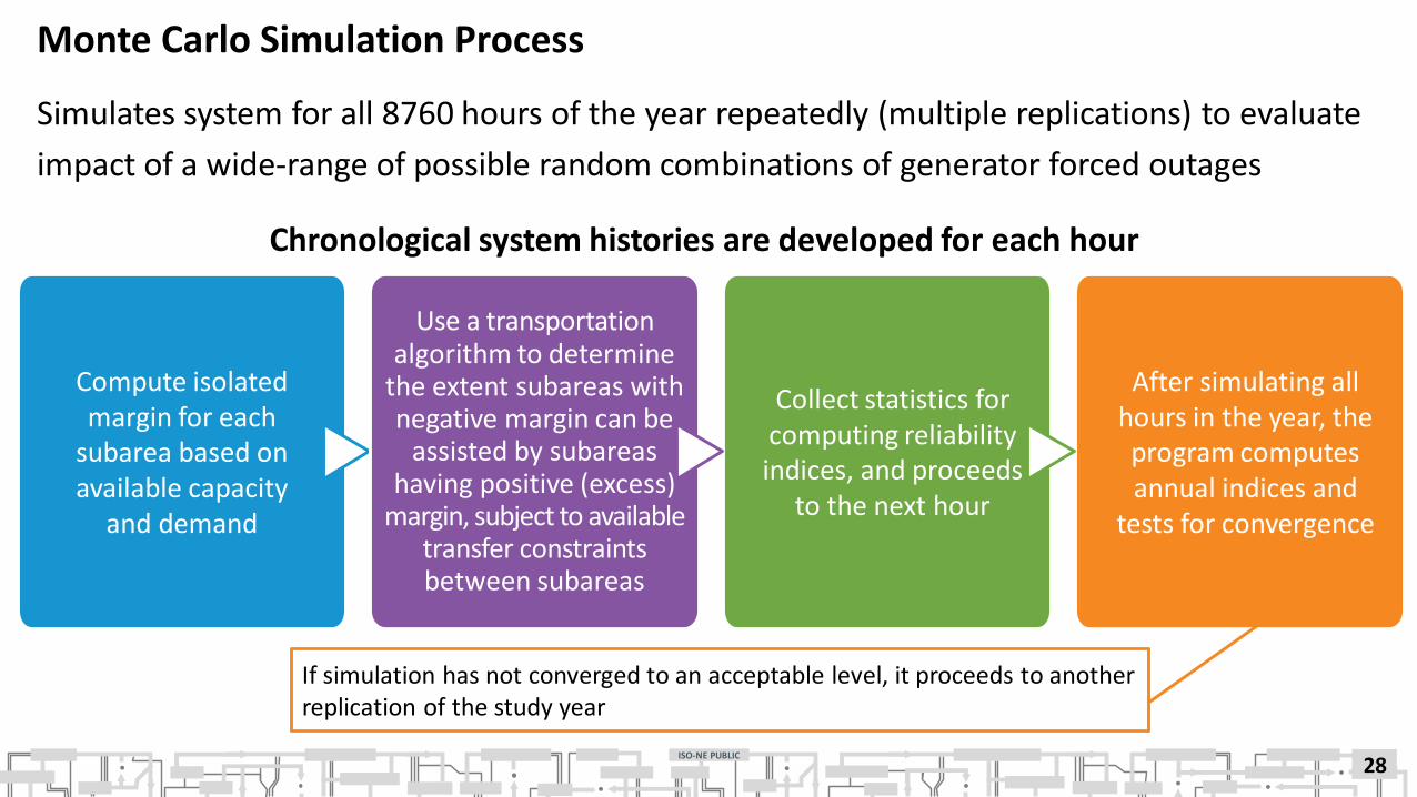
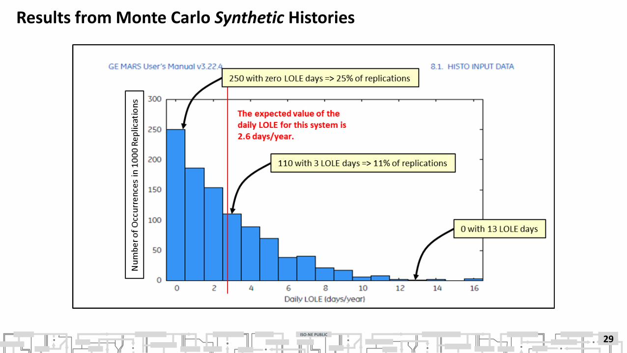
Monte Carlo Simulation Process

Simulates system for all 8760 hours of the year repeatedly (multiple replications) to evaluate

impact of a wide-range of possible random combinations of generator forced outages

28

Compute isolated margin for each

subarea based on available capacity

and demand

Use a transportation algorithm to determine

the extent subareas with negative margin can be

assisted by subareas having positive (excess)

margin, subject to available transfer constraints between subareas

Collect statistics for computing reliability indices, and proceeds

to the next hour

After simulating all hours in the year, the program computes annual indices and

tests for convergence

If simulation has not converged to an acceptable level, it proceeds to another replication of the study year

Chronological system histories are developed for each hour

ISO-NE PUBLIC

Results from Monte Carlo Synthetic Histories

29

ISO-NE PUBLIC

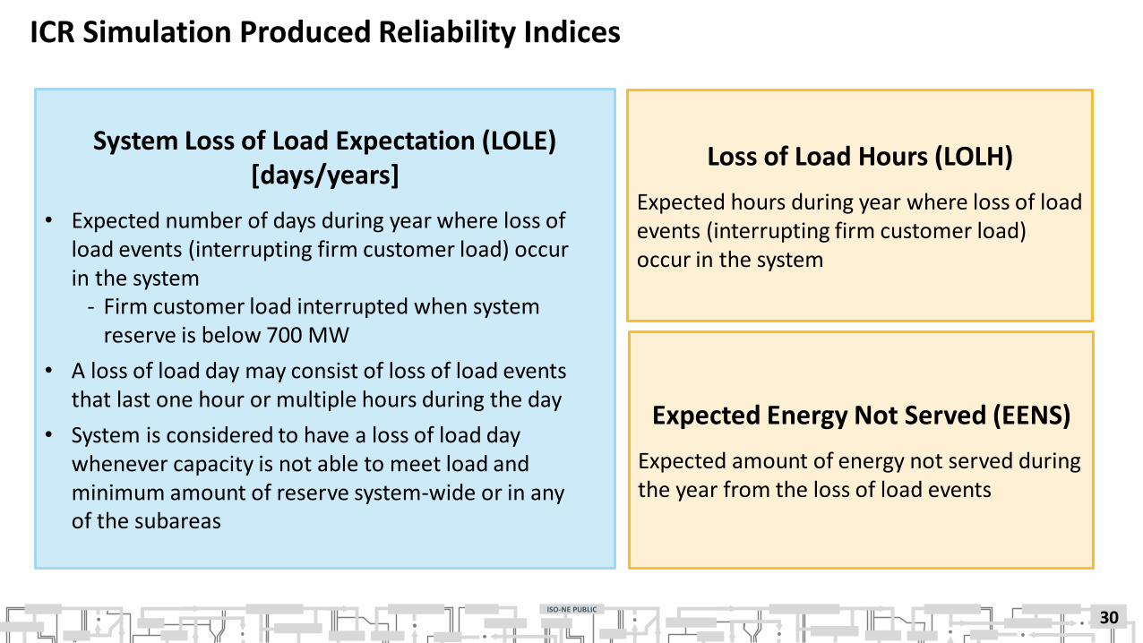
ICR Simulation Produced Reliability Indices

30

System Loss of Load Expectation (LOLE) [days/years]

• Expected number of days during year where loss of load events (interrupting firm customer load) occur in the system

- Firm customer load interrupted when system reserve is below 700 MW

• A loss of load day may consist of loss of load events that last one hour or multiple hours during the day

• System is considered to have a loss of load day whenever capacity is not able to meet load and minimum amount of reserve system-wide or in any of the subareas

Loss of Load Hours (LOLH)

Expected hours during year where loss of load events (interrupting firm customer load) occur in the system

Expected Energy Not Served (EENS)

Expected amount of energy not served duringthe year from the loss of load events

ISO-NE PUBLIC

System and Locational Capacity Requirements

31

ISO-NE PUBLIC

System-Wide and Zonal Requirements

For each FCM auction, ISO establishes:

32

System-Wide ICR Locational Requirements

Minimum amount of resources needed system-wide to meet the reliability target

Given the total amount of resources needed for the system, where should these resources be located within the system to reflect possible transmission bottle necks

Determine without assuming transmission bottle necks (one bus system)

Minimum requirement established for areas with limited import capability

Maximum requirement established for areas with limited export capability

ISO-NE PUBLIC

Calculating Installed Capacity Requirement

Using General Electric (GE) Multi-Area Reliability Simulation (MARS) model, the ISO

determines system loss-of-load expectation (LOLE) for given set of inputs

• If model determines system is:

‒ Less reliable than reliability criterion (LOLE > 0.1 days per year), proxy unit(s) are added

‒ More reliable than reliability criterion (LOLE < 0.1 days per year), load is increased so that LOLE

equals 0.1 days per year

• Additional load is termed Additional Load Carrying Capability (ALCC)

‒ Amount of extra load that can be served by surplus capacity resources

• ICR can then be calculated (notice the inputs are also used in this calculation)

33

𝐼𝑛𝑠𝑡𝑎𝑙𝑙𝑒𝑑 𝐶𝑎𝑝𝑎𝑐𝑖𝑡𝑦 𝑅𝑒𝑞𝑢𝑖𝑟𝑒𝑚𝑒𝑛𝑡 𝐼𝐶𝑅 =𝐶𝑎𝑝𝑎𝑐𝑖𝑡𝑦 − 𝑇𝑖𝑒 𝐵𝑒𝑛𝑒𝑓𝑖𝑡𝑠 − 𝑂𝑃4 𝐿𝑜𝑎𝑑 𝑅𝑒𝑙𝑖𝑒𝑓

1 +𝑨𝒅𝒅𝒊𝒕𝒊𝒐𝒏𝒂𝒍 𝑳𝒐𝒂𝒅 𝑪𝒂𝒓𝒓𝒚𝒊𝒏𝒈 𝑪𝒂𝒑𝒂𝒃𝒊𝒍𝒊𝒕𝒚

𝐴𝑛𝑛𝑢𝑎𝑙 𝑃𝑒𝑎𝑘 𝐿𝑜𝑎𝑑

+ 𝐻𝑄𝐼𝐶𝐶𝑠

ISO-NE PUBLIC

Net Installed Capacity Requirement

• Tie benefits from Hydro Québec Phase II Interconnection Capability Credits (HQICCs)

are allocated to specific entities holding contractual rights to this interconnection,

and monetized as credits in the form of reduced capacity requirements

• When referencing New England’s Installed Capacity Requirement, we generally mean the

Net Installed Capacity Requirement

34

𝑁𝑒𝑡 𝐼𝑛𝑠𝑡𝑎𝑙𝑙𝑒𝑑 𝐶𝑎𝑝𝑎𝑐𝑖𝑡𝑦 𝑅𝑒𝑞𝑢𝑖𝑟𝑒𝑚𝑒𝑛𝑡 𝐼𝐶𝑅 =𝐶𝑎𝑝𝑎𝑐𝑖𝑡𝑦 − 𝑇𝑖𝑒 𝐵𝑒𝑛𝑒𝑓𝑖𝑡𝑠 − 𝑂𝑃4 𝐿𝑜𝑎𝑑 𝑅𝑒𝑙𝑖𝑒𝑓

1 +𝐴𝐿𝐶𝐶

𝐴𝑛𝑛𝑢𝑎𝑙 𝑃𝑒𝑎𝑘 𝐿𝑜𝑎𝑑

𝑁𝑒𝑡 𝐼𝑛𝑠𝑡𝑎𝑙𝑙𝑒𝑑 𝐶𝑎𝑝𝑎𝑐𝑖𝑡𝑦 𝑅𝑒𝑞𝑢𝑖𝑟𝑒𝑚𝑒𝑛𝑡 𝑁𝑒𝑡 𝐼𝐶𝑅 = 𝐼𝑛𝑠𝑡𝑎𝑙𝑙𝑒𝑑 𝐶𝑎𝑝𝑎𝑐𝑖𝑡𝑦 𝑅𝑒𝑞𝑢𝑖𝑟𝑒𝑚𝑒𝑛𝑡 𝐼𝐶𝑅 − 𝐻𝑄𝐼𝐶𝐶𝑠

ISO-NE PUBLIC

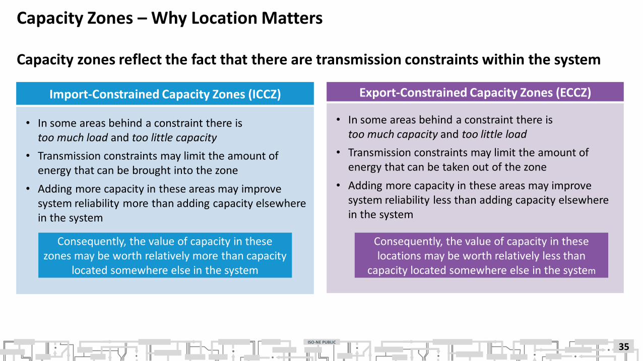
Capacity Zones – Why Location Matters

Capacity zones reflect the fact that there are transmission constraints within the system

35

Import-Constrained Capacity Zones (ICCZ)

• In some areas behind a constraint there is too much load and too little capacity

• Transmission constraints may limit the amount of energy that can be brought into the zone

• Adding more capacity in these areas may improve system reliability more than adding capacity elsewhere in the system

Export-Constrained Capacity Zones (ECCZ)

• In some areas behind a constraint there istoo much capacity and too little load

• Transmission constraints may limit the amount of energy that can be taken out of the zone

• Adding more capacity in these areas may improve system reliability less than adding capacity elsewhere in the system

Consequently, the value of capacity in these zones may be worth relatively more than capacity

located somewhere else in the system

Consequently, the value of capacity in these locations may be worth relatively less than

capacity located somewhere else in the system

ISO-NE PUBLIC

Identifying Potential Zonal Boundaries

• ISO performs an annual assessment of transmission transfer capabilities to identify

potential zonal boundaries and associated transfer limits between those boundaries for

capacity zone modeling in the Forward Capacity Auction

• Changes in power grid are also assessed and would include updates to transmission

topology, retirements of existing resources, and addition of new capacity resources

36

ISO-NE PUBLIC

Capacity ZonesFCA 10

Capacity ZonesFCA 11, 12, & 13

Examples of Capacity Zones Used in Past FCAs

• ISO analyzes and identifies capacity

zones for every Capacity Commitment

Period (CCP)

• Once established for a CCP, capacity

zones will not change

• Capacity zones provide locational

market signals

37

Export-Constrained

Import-ConstrainedRest of

Pool

Rest ofPool

Import-Constrained

ISO-NE PUBLIC

Zonal Requirements Determination

• ISO uses the same GE MARS model and assumptions used for the ICR calculation to

determine expected capacity zone demand requirements for Capacity Commitment

Periods where internal constraints are modeled

• Two area model (Capacity Zone vs. Rest-of-Pool)

38

Rest-of-Pool into export-constrained capacity zone

until system LOLE reaches at 0.105 days per year

(indicating interface is binding)

Import-constrained capacity zone into Rest-of-Pool

until system LOLE reaches at 0.105 days per year

(indicating interface is binding)

For import-constrained zone this point is called

local-resource adequacy requirement (LRA)

For export-constrained zone this point is called

maximum capacity limit (MCL)

With amount of capacity in system being held constant at ICR level, capacity is transferred from:

ISO-NE PUBLIC

FCM System and Zonal Demand Curves

39

ISO-NE PUBLIC

Demand Curves: Marginal Reliability Impact Approach

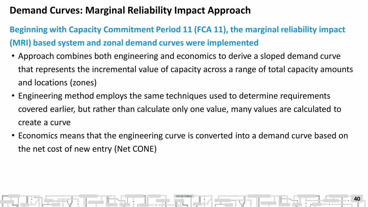
Beginning with Capacity Commitment Period 11 (FCA 11), the marginal reliability impact

(MRI) based system and zonal demand curves were implemented

• Approach combines both engineering and economics to derive a sloped demand curve

that represents the incremental value of capacity across a range of total capacity amounts

and locations (zones)

• Engineering method employs the same techniques used to determine requirements

covered earlier, but rather than calculate only one value, many values are calculated to

create a curve

• Economics means that the engineering curve is converted into a demand curve based on

the net cost of new entry (Net CONE)

40

ISO-NE PUBLIC

Marginal Reliability Impact

• Represents incremental impacts on system reliability

‒ Reflects incremental improvement in reliability associated with adding incremental capacity

‒ Calculated at various capacity levels in 10 MW blocks

• Requires hundreds of simulations for each curve

• MRI curve is derived using the same MARS model and inputs used to derive the ICR

requirements covered earlier

41

ISO-NE PUBLIC

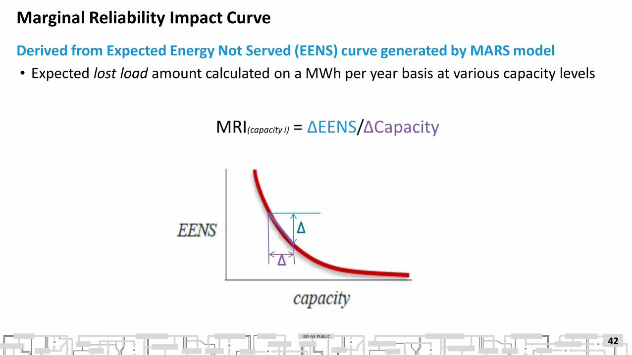
Marginal Reliability Impact Curve

Derived from Expected Energy Not Served (EENS) curve generated by MARS model

• Expected lost load amount calculated on a MWh per year basis at various capacity levels

42

ISO-NE PUBLIC

Marginal Reliability Impact Curve Characteristics

43

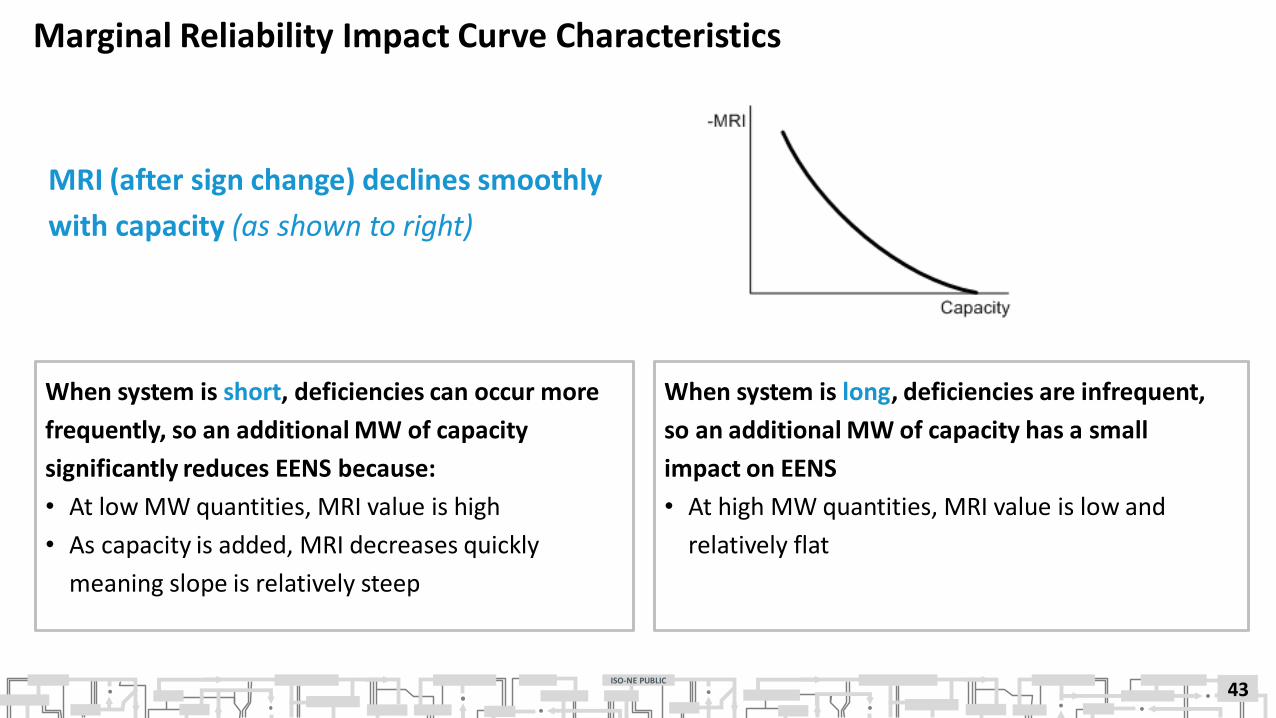
MRI (after sign change) declines smoothly

with capacity (as shown to right)

When system is short, deficiencies can occur more

frequently, so an additional MW of capacity

significantly reduces EENS because:

• At low MW quantities, MRI value is high

• As capacity is added, MRI decreases quickly

meaning slope is relatively steep

When system is long, deficiencies are infrequent,

so an additional MW of capacity has a small

impact on EENS

• At high MW quantities, MRI value is low and

relatively flat

ISO-NE PUBLIC

Economics of a MRI Based Demand Curve

System MRI curve is converted into a price-quantity curve

• This is done by scaling curve so price at intersection of Net Installed Capacity Requirement

(ICR) is equal to net cost of new entry (Net CONE)

44

ISO-NE PUBLIC

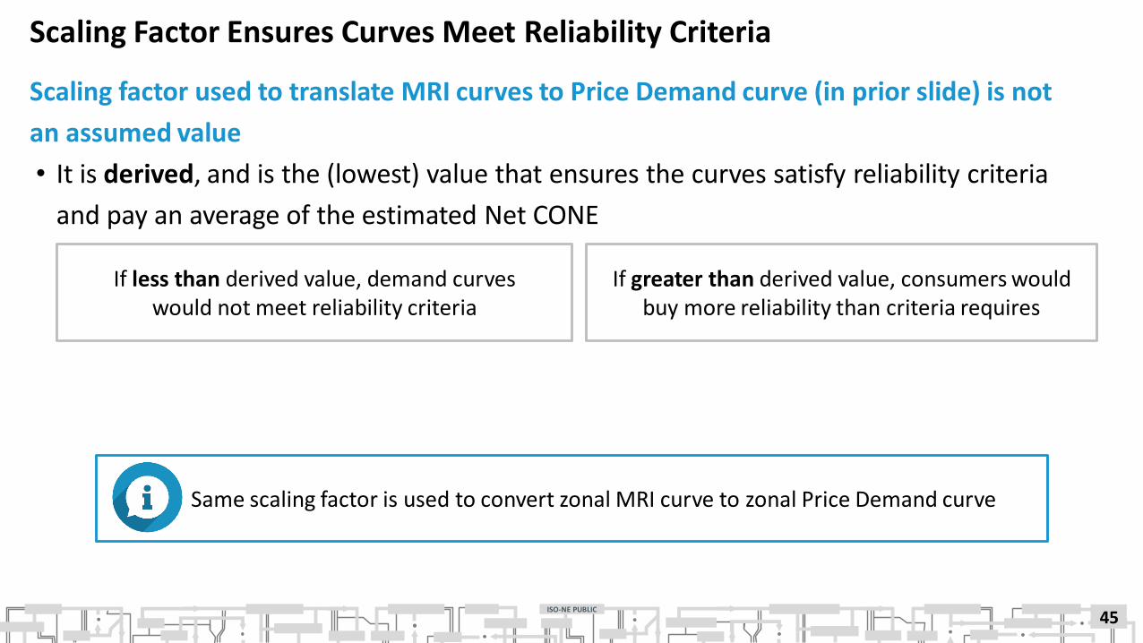
Scaling Factor Ensures Curves Meet Reliability Criteria

Scaling factor used to translate MRI curves to Price Demand curve (in prior slide) is not

an assumed value

• It is derived, and is the (lowest) value that ensures the curves satisfy reliability criteria

and pay an average of the estimated Net CONE

45

Same scaling factor is used to convert zonal MRI curve to zonal Price Demand curve

If less than derived value, demand curves would not meet reliability criteria

If greater than derived value, consumers would buy more reliability than criteria requires

ISO-NE PUBLIC

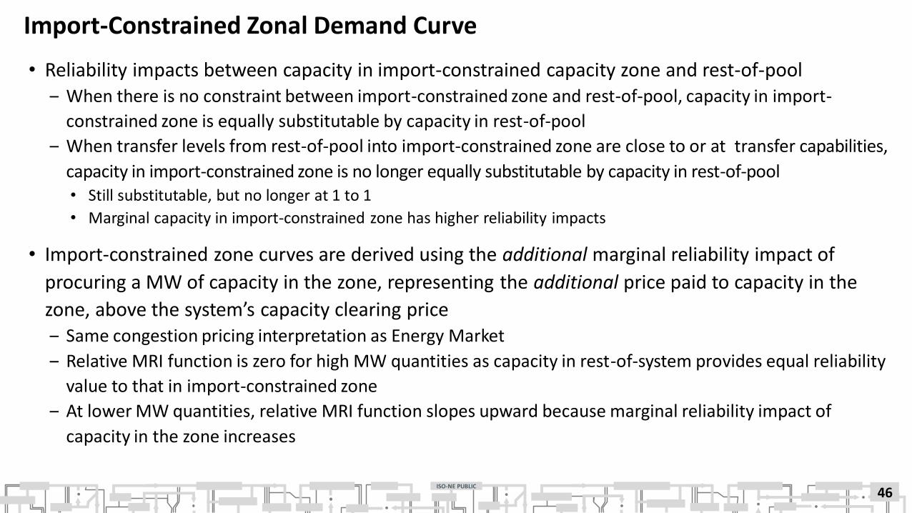
Import-Constrained Zonal Demand Curve

• Reliability impacts between capacity in import-constrained capacity zone and rest-of-pool‒ When there is no constraint between import-constrained zone and rest-of-pool, capacity in import-

constrained zone is equally substitutable by capacity in rest-of-pool

‒ When transfer levels from rest-of-pool into import-constrained zone are close to or at transfer capabilities,

capacity in import-constrained zone is no longer equally substitutable by capacity in rest-of-pool• Still substitutable, but no longer at 1 to 1

• Marginal capacity in import-constrained zone has higher reliability impacts

• Import-constrained zone curves are derived using the additional marginal reliability impact of

procuring a MW of capacity in the zone, representing the additional price paid to capacity in the

zone, above the system’s capacity clearing price‒ Same congestion pricing interpretation as Energy Market

‒ Relative MRI function is zero for high MW quantities as capacity in rest-of-system provides equal reliability

value to that in import-constrained zone

‒ At lower MW quantities, relative MRI function slopes upward because marginal reliability impact of

capacity in the zone increases

46

ISO-NE PUBLIC

Import-Constrained Zonal Demand Curve, continued

Import-constrained zonal demand curve is generated using similar process for developing

system-wide demand curve

• Generate EENS curve for various zonal capacity levels using two area model

(import-constrained zone vs. rest-of-pool)

‒ Import capability is adjusted if zonal TSA requirement is greater than LRA requirement

• Derive MRI curve from EENS curve

• Translate MRI curve into demand curve using same Scaling Factor used for system-wide

demand curve

47

= (N-1 limit) – max(TSA-LRA,0)

ISO-NE PUBLIC

Import-Constrained Zonal Demand Curve (FCA 11 Example for SENE)

48

ISO-NE PUBLIC

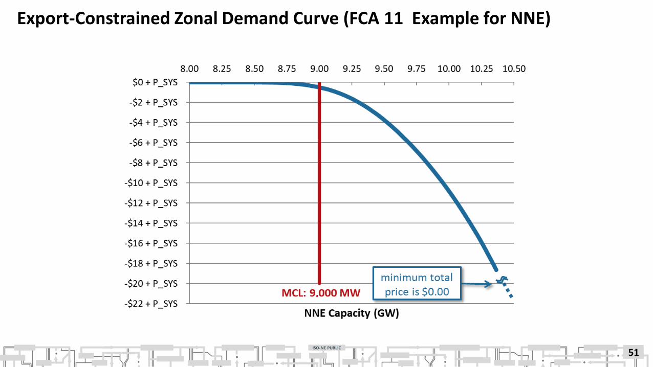
Export-Constrained Zonal Demand Curve

• Reliability impacts between capacity in export-constrained capacity zone and rest-of-pool‒ When there is no constraint between export-constrained zone and rest-of-pool, capacity in rest-of-pool is

equally substitutable by capacity in export-constrained zone

‒ When transfer levels from export-constrained zone into rest-of-pool are close to or at transfer capabilities,

capacity in rest-of-pool is no longer equally substitutable by capacity in export-constrained zone • Still substitutable, but no longer at 1 to 1

• Marginal capacity in export-constrained zone has lower reliability impacts

• Export-constrained zone curves are derived using the additional marginal reliability impact of

procuring a MW of capacity in the zone, representing the additional price paid to capacity in the

zone, above the system’s capacity clearing price‒ Additional price is negative as capacity in export-constrained zone has lower reliability impact due to constraints

‒ Relative MRI function is zero for lower MW quantities as capacity in export-constrained zone provides

equal reliability value to that in rest-of-pool

‒ At higher MW quantities, relative MRI function slopes downward because marginal reliability impact of

capacity in export-constrained zone decreases

49

ISO-NE PUBLIC

Export-Constrained Zonal Demand Curve, continued

Export-constrained zonal demand curve is generated using similar process for developing

system-wide demand curve

• Generate EENS curve for various zonal capacity levels using two area model

(export-constrained zone vs. rest-of-pool)

• Derive MRI curve from EENS curve

• Translate MRI curve into Demand Curve using same Scaling Factor used for system-wide

demand curve

50

ISO-NE PUBLIC

Export-Constrained Zonal Demand Curve (FCA 11 Example for NNE)

51

ISO-NE PUBLIC

Installed Capacity Requirement Assumption Developments

52

ISO-NE PUBLIC

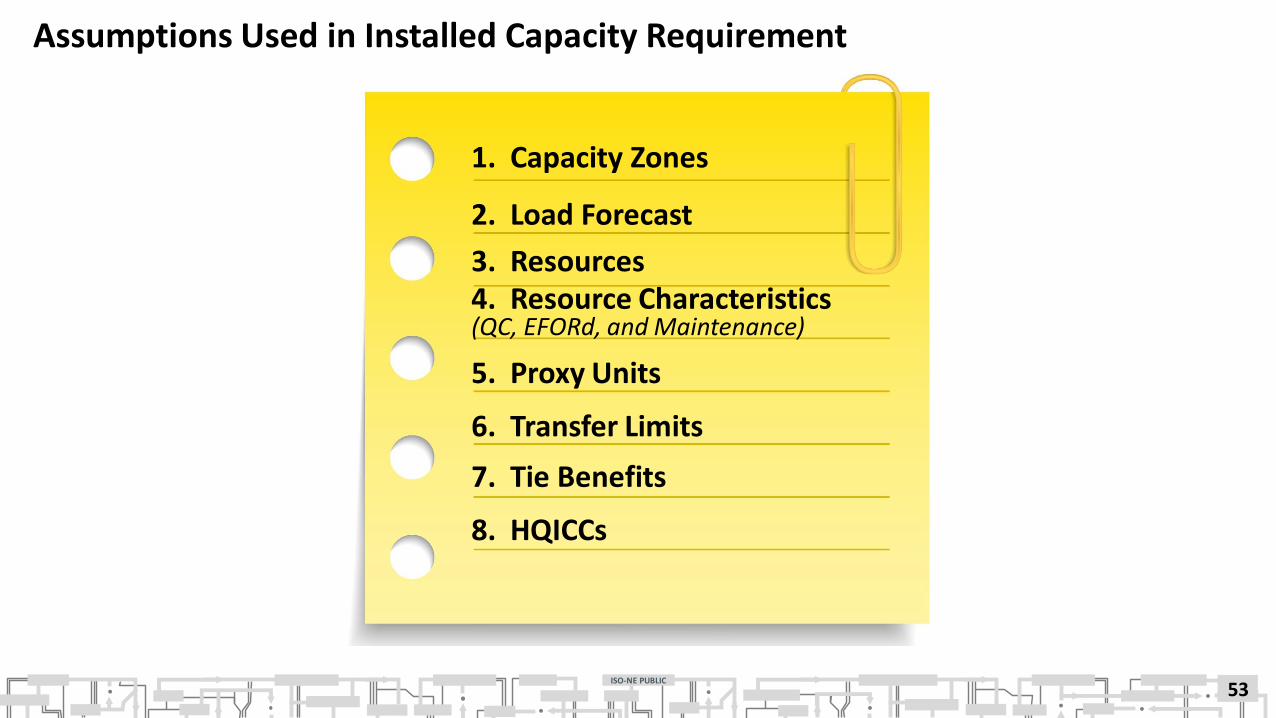
Assumptions Used in Installed Capacity Requirement

53

1. Capacity Zones

2. Load Forecast

3. Resources4. Resource Characteristics(QC, EFORd, and Maintenance)

5. Proxy Units

6. Transfer Limits

7. Tie Benefits

8. HQICCs

ISO-NE PUBLIC

Load Forecast Used for Installed Capacity Requirement Calculation

• Latest load forecast is used in ICR development and updated on annual basis

‒ Load forecast goes through a stakeholder process (LFC, DGFWG, EEFWG, RC, PAC)

‒ Published in CELT report: System Planning > Plans and Studies > CELT Reports

• Component of Load Forecast Model

‒ Annual peak demands

‒ Distributions of weekly peak loads (Load Forecast Uncertainty due to Weather)

‒ Hourly gross load shape (2002)

‒ Hourly peak load reduction from BTM PV

• Methodology and assumptions for the Load Forecast are developed by the ISO

based on guidelines in the Market Rule and discussions with stakeholders

throughout the committee processes

54

ISO-NE PUBLIC

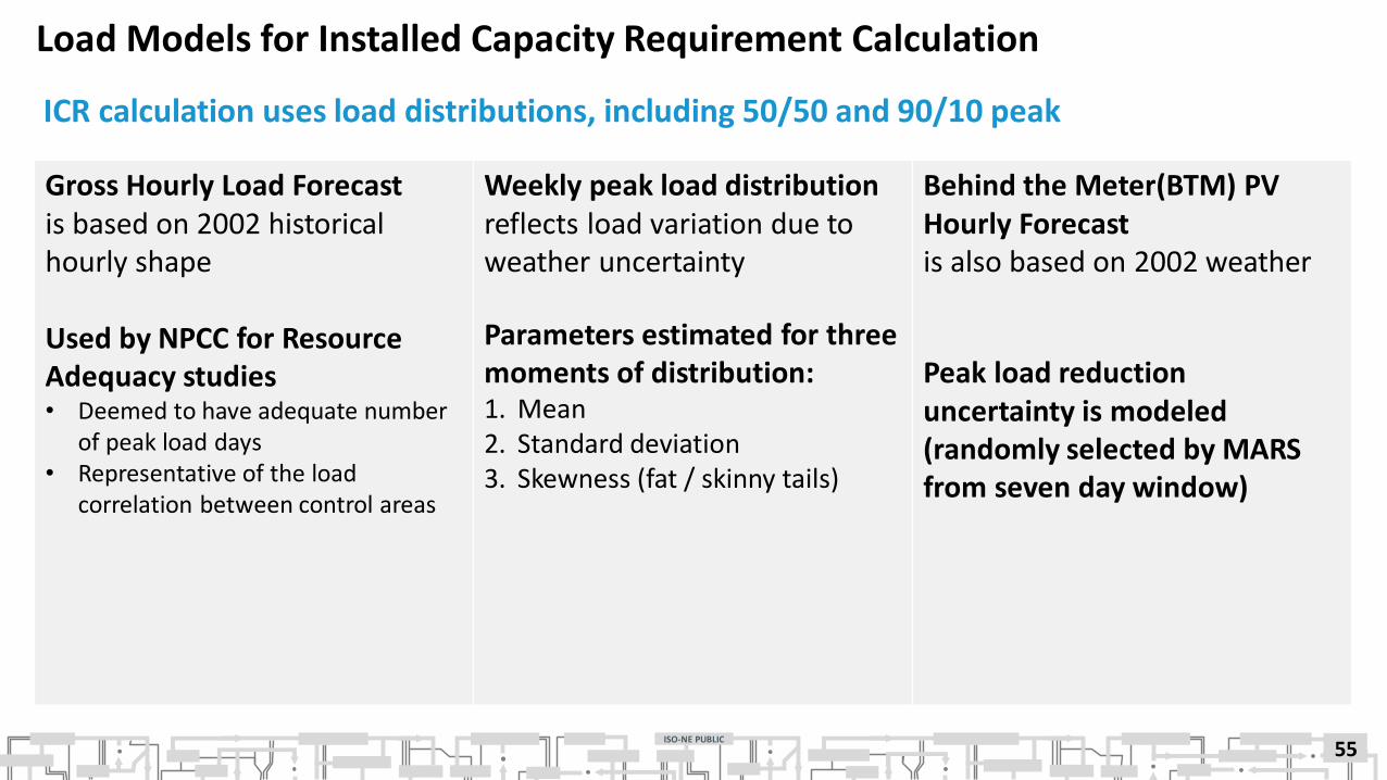
Load Models for Installed Capacity Requirement Calculation

ICR calculation uses load distributions, including 50/50 and 90/10 peak

55

Gross Hourly Load Forecast is based on 2002 historicalhourly shape

Used by NPCC for Resource Adequacy studies• Deemed to have adequate number

of peak load days• Representative of the load

correlation between control areas

Weekly peak load distribution reflects load variation due to weather uncertainty

Parameters estimated for three moments of distribution: 1. Mean2. Standard deviation3. Skewness (fat / skinny tails)

Behind the Meter(BTM) PV Hourly Forecast is also based on 2002 weather

Peak load reduction uncertainty is modeled (randomly selected by MARS from seven day window)

ISO-NE PUBLIC

Existing Capacity Resources

When calculating ICR-Related Values, model utilizes qualified capacity of Existing Capacity Resources

56

Qualified Existing Non-Intermittent Generating

Capacity Resources

Qualified Existing Intermittent Power

Resources

Qualified Existing Import Capacity

Resources

Qualified Existing Demand Capacity Resources

(DCR)

• On-Peak (Passive)• Seasonal Peak (Passive)• Active Demand Capacity

Resource (ADCR)

Generation Imports Demand Response

ISO-NE PUBLIC

Capacity Resource Data

• Only FCM resources are modeled‒ Resources that participate in Energy Market only are not included

• Intermittent Power Resources

‒ Scheduled maintenance is not modeled specifically because it is considered to be reflected

in resource rating

‒ Forced outages are not modeled specifically because it is considered to be reflected

in resource rating

‒ Resource rating is based on the actual MW output during the

reliability hours, therefore maintenance and outages have been

accounted for

57

ISO-NE PUBLIC

Capacity Resource Data, continued

Non-intermittent existing resources are modeled within ICR-related value calculations at their summer Qualified Capacity (QC) rating, a forced outage rate (EFORd), and scheduled maintenance outages• Both are based on historical data; most recent 5-years of data

58

Scheduled maintenance outage assumptions

Each generating units annual weeks of maintenance are used and based on a five-year average of each generator’s actual historical average of planned and maintenance outages (i.e., outages scheduled at least 14 days in advance)

Forced outage assumptions

• Each generating units equivalent forced outage rate - demand is used and is based on a five-year average of submitted Generating Availability Data System (GADS) data

• EFORd is a outage parameter that best describe units that are infrequently operated

If unit is not operational for a full 5 years, NERC-GADS class average data

is used to substitute for the missing EFORd and maintenance outage assumptions.

ISO-NE PUBLIC

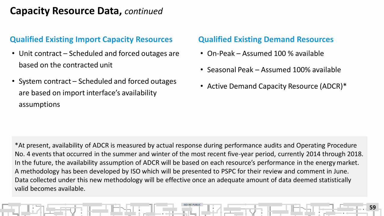
Qualified Existing Import Capacity Resources Qualified Existing Demand Resources

Capacity Resource Data, continued

• Unit contract – Scheduled and forced outages are

based on the contracted unit

• System contract – Scheduled and forced outages

are based on import interface’s availability

assumptions

• On-Peak – Assumed 100 % available

• Seasonal Peak – Assumed 100% available

• Active Demand Capacity Resource (ADCR)*

59

*At present, availability of ADCR is measured by actual response during performance audits and Operating Procedure No. 4 events that occurred in the summer and winter of the most recent five-year period, currently 2014 through 2018. In the future, the availability assumption of ADCR will be based on each resource’s performance in the energy market. A methodology has been developed by ISO which will be presented to PSPC for their review and comment in June. Data collected under this new methodology will be effective once an adequate amount of data deemed statistically valid becomes available.

ISO-NE PUBLIC

New Capacity Resources

• Non-commercial resources that cleared in previous FCA(s) are modeled

‒ MW amount based on CSO (not QC)

‒ Maintenance weeks assumed based on US NERC-GADS class average for the resource technology

type

‒ EFORd assumed based on US NERC-GADS class average for resource technology type

• New Capacity Resources seeking qualification for the CCP in which ICR-Related Values are

being developed are not included in the model

60

For more information on NERC-GADS data: https://www.nerc.com/pa/RAPA/gads/Pages/Reports.aspx

ISO-NE PUBLIC

Why use proxy units when calculating ICR-Related Values?

What are proxy unit* characteristics?

Proxy Units

• Use of proxy units avoids an unjustified

increase or decrease in the system LOLE

that may result from assuming a specific

type of resource addition

• Proxy unit is effectively neutral to

ICR calculations

• 400 MW generator

• Scheduled outage – 4 weeks/year

• Forced outages – 5.47 EFORd

61

*Based on a study conducted in 2014. ISO plans to conduct a new study this year. Copy of the presentation is available at https://www.iso-ne.com/static-

assets/documents/committees/comm_wkgrps/relblty_comm/pwrsuppln_comm/mtrls/2014/may222014/proxy_unit_2014_study.pdf

ISO-NE PUBLIC

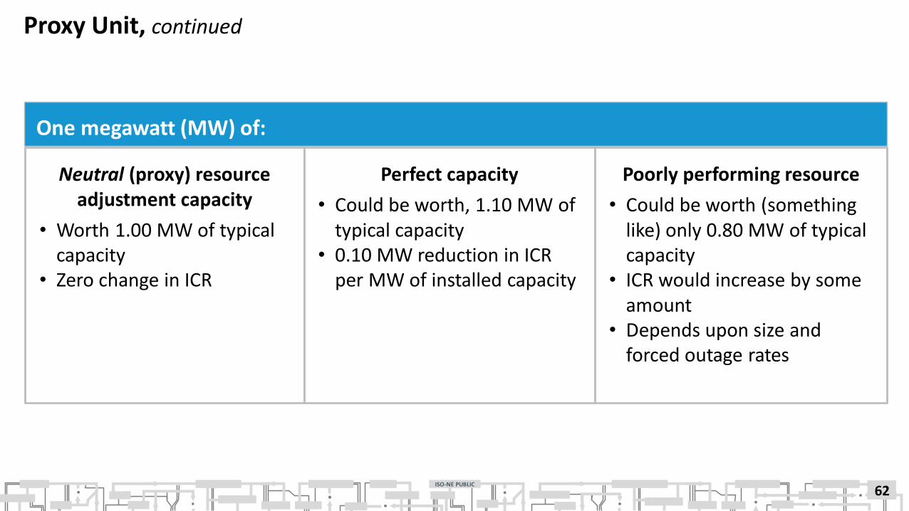
Proxy Unit, continued

One megawatt (MW) of:

62

Neutral (proxy) resource adjustment capacity

• Worth 1.00 MW of typical capacity

• Zero change in ICR

Perfect capacity

• Could be worth, 1.10 MW of typical capacity

• 0.10 MW reduction in ICR per MW of installed capacity

Poorly performing resource

• Could be worth (something like) only 0.80 MW of typical capacity

• ICR would increase by some amount

• Depends upon size and forced outage rates

ISO-NE PUBLIC

Transmission Limits

Interface limits are determined pursuant to ISO Tariff Section II, Attachment K

Use network models that include all resources, existing transmission lines and proposed

transmission lines that the ISO determines, in accordance with Section III.12.6, will be in

service no later than the first day of the relevant Capacity Commitment Period. The

transmission interface limits shall be established, using deterministic analyses, at levels that

provide acceptable thermal, voltage and stability performance of the system both with all

lines in service and after any criteria contingency occurs as specified in ISO New England

Manuals and ISO New England Administrative Procedures.

63

ISO-NE PUBLIC

Transmission Limits, continued

• System ICR calculation do not model transmission constraints

• Capacity zone requirements (LRA and MCL) use the N-1 limit of the transmission interface

associated with capacity zone

• Import constrained capacity zone requirement (TSA) use N-1 and N-1-1 limits of the

transmission interface associated with capacity zone

• Tie Benefits study use both internal and external transmission interface (N-1)‒ External interfaces availability assumptions are based on historical maintenance and forced outages

‒ Currently the EFORd associated with external ties are:

64https://www.iso-ne.com/static-assets/documents/2018/04/a9_fca13_zonal_development.pdf

Update to table will be discussed at May 30, 2019 PSPC Meeting: https://www.iso-ne.com/event-details?eventId=137697

ISO-NE PUBLIC

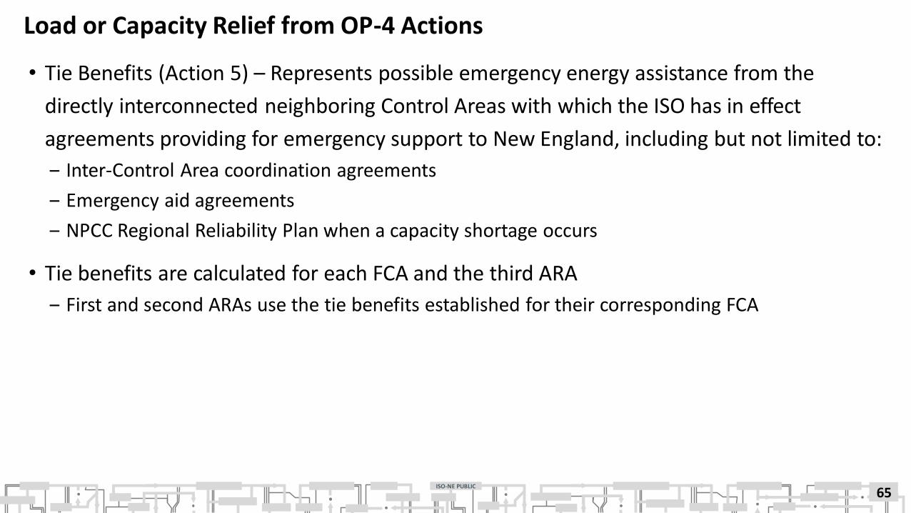
Load or Capacity Relief from OP-4 Actions

• Tie Benefits (Action 5) – Represents possible emergency energy assistance from the

directly interconnected neighboring Control Areas with which the ISO has in effect

agreements providing for emergency support to New England, including but not limited to:

‒ Inter-Control Area coordination agreements

‒ Emergency aid agreements

‒ NPCC Regional Reliability Plan when a capacity shortage occurs

• Tie benefits are calculated for each FCA and the third ARA

‒ First and second ARAs use the tie benefits established for their corresponding FCA

65

ISO-NE PUBLIC

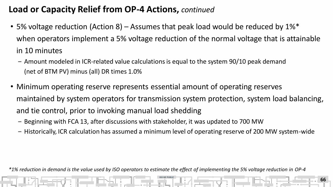
Load or Capacity Relief from OP-4 Actions, continued

• 5% voltage reduction (Action 8) – Assumes that peak load would be reduced by 1%*

when operators implement a 5% voltage reduction of the normal voltage that is attainable

in 10 minutes

‒ Amount modeled in ICR-related value calculations is equal to the system 90/10 peak demand

(net of BTM PV) minus (all) DR times 1.0%

• Minimum operating reserve represents essential amount of operating reserves

maintained by system operators for transmission system protection, system load balancing,

and tie control, prior to invoking manual load shedding

‒ Beginning with FCA 13, after discussions with stakeholder, it was updated to 700 MW

‒ Historically, ICR calculation has assumed a minimum level of operating reserve of 200 MW system-wide

66

*1% reduction in demand is the value used by ISO operators to estimate the effect of implementing the 5% voltage reduction in OP-4

ISO-NE PUBLIC

OP-4 Resources and Total Resources Needed to Meet Resource AdequacyCriterion

67

Total resources needed to meet resource adequacy criterion

OP-4 Resources

OP-4 Resources

New England Installed Capacity including External

Capacity Purchases

Operating Reserve

Operating Reserve

“Fewer” OP-4 Events

“More” OP-4 Events

New England Installed Capacity including External

Capacity Purchases

ISO-NE PUBLIC

Tie Benefits

68

ISO-NE PUBLIC

Tie Benefits

• In the event of a capacity shortage in New England, tie benefits reflect the amount of

emergency assistance assumed to be available from neighboring control areas

• Tie benefits are an input in the determination of ICR-Related Values and displace

(i.e., lower) the capacity amount needed to meet reliability criterion by an almost

one-to-one ratio

• Tie benefits from Hydro Québec Phase II interconnection, called Interconnection Capability

Credits (HQICCs) are allocated to specific entities holding contractual rights to this

interconnection, and monetized as credits in the form of reduced capacity requirements

69

ISO-NE PUBLIC

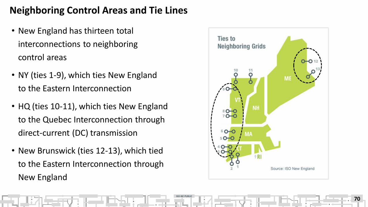
Neighboring Control Areas and Tie Lines

• New England has thirteen total

interconnections to neighboring

control areas

• NY (ties 1-9), which ties New England

to the Eastern Interconnection

• HQ (ties 10-11), which ties New England

to the Quebec Interconnection through

direct-current (DC) transmission

• New Brunswick (ties 12-13), which tied

to the Eastern Interconnection through

New England

70

ISO-NE PUBLIC

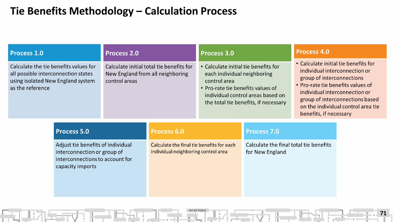
Tie Benefits Methodology – Calculation Process

71

ISO-NE PUBLIC

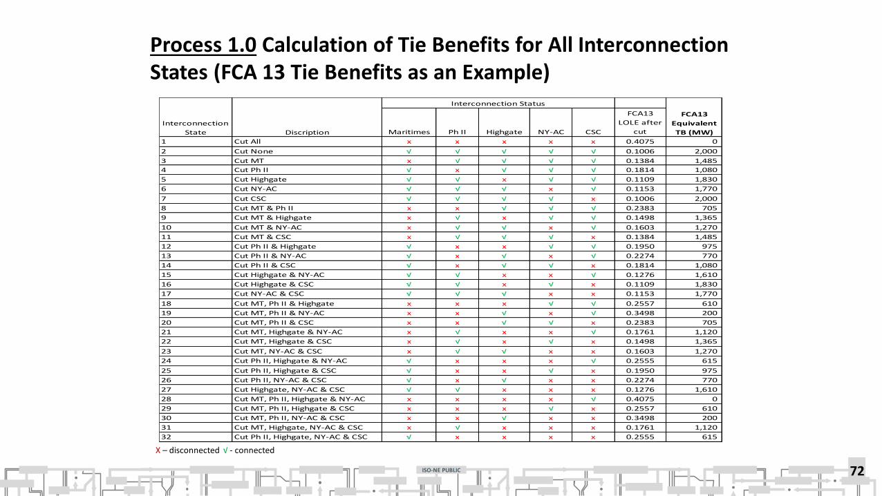
Process 1.0 Calculation of Tie Benefits for All Interconnection States (FCA 13 Tie Benefits as an Example)

72

X – disconnected √ - connected

Maritimes Ph II Highgate NY-AC CSC

FCA13

LOLE after

cut

1 Cut All x x x x x 0.4075 0

2 Cut None √ √ √ √ √ 0.1006 2,000

3 Cut MT x √ √ √ √ 0.1384 1,485

4 Cut Ph II √ x √ √ √ 0.1814 1,080

5 Cut Highgate √ √ x √ √ 0.1109 1,830

6 Cut NY-AC √ √ √ x √ 0.1153 1,770

7 Cut CSC √ √ √ √ x 0.1006 2,000

8 Cut MT & Ph II x x √ √ √ 0.2383 705

9 Cut MT & Highgate x √ x √ √ 0.1498 1,365

10 Cut MT & NY-AC x √ √ x √ 0.1603 1,270

11 Cut MT & CSC x √ √ √ x 0.1384 1,485

12 Cut Ph II & Highgate √ x x √ √ 0.1950 975

13 Cut Ph II & NY-AC √ x √ x √ 0.2274 770

14 Cut Ph II & CSC √ x √ √ x 0.1814 1,080

15 Cut Highgate & NY-AC √ √ x x √ 0.1276 1,610

16 Cut Highgate & CSC √ √ x √ x 0.1109 1,830

17 Cut NY-AC & CSC √ √ √ x x 0.1153 1,770

18 Cut MT, Ph II & Highgate x x x √ √ 0.2557 610

19 Cut MT, Ph II & NY-AC x x √ x √ 0.3498 200

20 Cut MT, Ph II & CSC x x √ √ x 0.2383 705

21 Cut MT, Highgate & NY-AC x √ x x √ 0.1761 1,120

22 Cut MT, Highgate & CSC x √ x √ x 0.1498 1,365

23 Cut MT, NY-AC & CSC x √ √ x x 0.1603 1,270

24 Cut Ph II, Highgate & NY-AC √ x x x √ 0.2555 615

25 Cut Ph II, Highgate & CSC √ x x √ x 0.1950 975

26 Cut Ph II, NY-AC & CSC √ x √ x x 0.2274 770

27 Cut Highgate, NY-AC & CSC √ √ x x x 0.1276 1,610

28 Cut MT, Ph II, Highgate & NY-AC x x x x √ 0.4075 0

29 Cut MT, Ph II, Highgate & CSC x x x √ x 0.2557 610

30 Cut MT, Ph II, NY-AC & CSC x x √ x x 0.3498 200

31 Cut MT, Highgate, NY-AC & CSC x √ x x x 0.1761 1,120

32 Cut Ph II, Highgate, NY-AC & CSC √ x x x x 0.2555 615

Interconnection

State Discription

Interconnection Status

FCA13

Equivalent

TB (MW)

ISO-NE PUBLIC

Process 2.0 Calculation of Initial Total Tie Benefits

Compare state 1 (without any ties) and state 2 (with all the ties)

• TB_total_initial = 2,000 MW

• This value is subject to the adjustment later to account for imports

73

ISO-NE PUBLIC

Process 3.0 Calculation of Tie Benefits for Neighboring Control Areas

All interconnections connected to a given neighboring control area are grouped together to represent the state of interconnection between New England and that neighboring control area. The simple average of values for all the interconnection states represents the tie benefits of the target neighboring control area (four states for each area)

Tie Benefits from Maritimes• 1 vs. 32 = 615 2 vs. 3 = 515 12 vs. 18 = 365 17 vs. 23 = 500• Average = 499 MW

Tie Benefits from Hydro Quebec• 1 vs. 23 = 1,270 2 vs. 12 = 1,025 3 vs. 18 = 875 17 vs. 32 = 1,155• Average = 1,081 MW

Tie Benefits from New York• 1 vs. 18 = 610 2 vs. 17 = 230 3 vs. 23 = 215 12 vs. 32 = 360• Average = 354 MW

Tie Benefits after Proration (since 499 + 1,081 + 354 = 1,934 ≠ 2,000)• TB_MTCA_initial = 2,000 * 499 / (499 +1,081 + 354) = 2,000 * 0.2579 = 516 MW• TB_HQCA_initial = 2,000 * 1,081 / (499 +1,081 + 354) = 2,000 * 0.5591 = 1,118 MW• TB_NYCA_initial = 2,000 * 354 / (499 + 1,081 + 354) = 2,000 * 0.1829 = 366 MW

74

ISO-NE PUBLIC

Process 4.0 Calculation of Tie Benefits for Individual or Group of Interconnections

Each individual interconnection or group of interconnections subject to the individual tie benefits contribution calculation is treated independently. The simple average of values for all the interconnection states represents tie benefits of the target interconnection or group of interconnections

Interconnections with Maritimes• No individual interconnections subject to the calculation

Interconnections with Quebec• Phase II and Highgate are subject to the calculation

• Phase II ‒ 1 vs. 31 = 1,120 2 vs. 4 = 920 3 vs. 8 = 780 5 vs. 12 = 855‒ 9 vs. 18 = 755 17 vs. 26 = 1,000 23 vs. 30 = 1,070 27 vs. 32 = 995‒ Average = 937 MW

• Highgate‒ 1 vs. 30 = 200 2 vs. 5 = 170 3 vs. 9 = 120 4 vs. 12 = 105‒ 8 vs. 18 = 95 17 vs. 27 = 160 23 vs. 31 = 150 26 vs. 32 = 155‒ Average = 144 MW

• Tie Benefits after proration (since 937 + 144 = 1,081 ≠ 1,118)‒ TB_Ph-II_initial = 1,118 * 937 / (937 + 144) = 1,118 * 0.8665 = 969 MW‒ TB_HG_initial = 1,118 * 144 / (937 + 144) = 1,118 * 0.1335 = 149 MW

75

ISO-NE PUBLIC

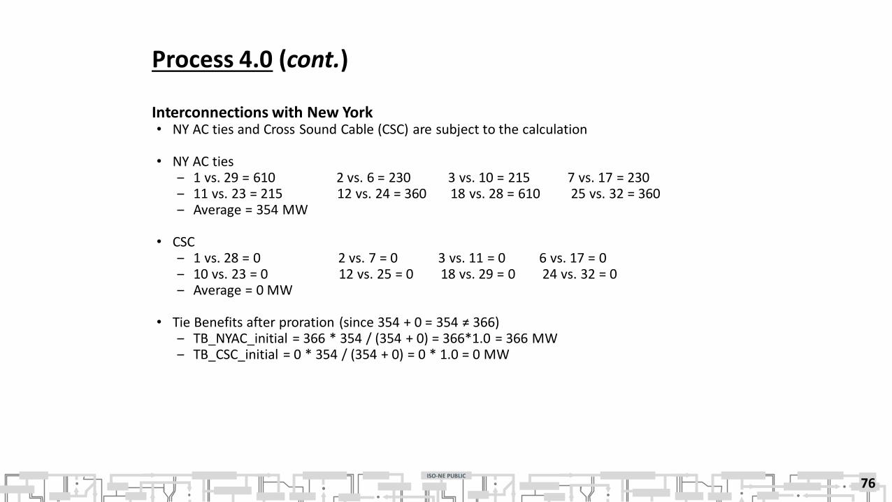
Process 4.0 (cont.)

Interconnections with New York• NY AC ties and Cross Sound Cable (CSC) are subject to the calculation

• NY AC ties‒ 1 vs. 29 = 610 2 vs. 6 = 230 3 vs. 10 = 215 7 vs. 17 = 230‒ 11 vs. 23 = 215 12 vs. 24 = 360 18 vs. 28 = 610 25 vs. 32 = 360‒ Average = 354 MW

• CSC‒ 1 vs. 28 = 0 2 vs. 7 = 0 3 vs. 11 = 0 6 vs. 17 = 0‒ 10 vs. 23 = 0 12 vs. 25 = 0 18 vs. 29 = 0 24 vs. 32 = 0‒ Average = 0 MW

• Tie Benefits after proration (since 354 + 0 = 354 ≠ 366)‒ TB_NYAC_initial = 366 * 354 / (354 + 0) = 366*1.0 = 366 MW‒ TB_CSC_initial = 0 * 354 / (354 + 0) = 0 * 1.0 = 0 MW

76

ISO-NE PUBLIC

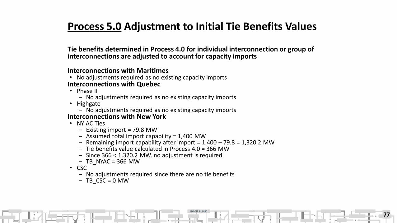
Process 5.0 Adjustment to Initial Tie Benefits Values

Tie benefits determined in Process 4.0 for individual interconnection or group of interconnections are adjusted to account for capacity imports

Interconnections with Maritimes• No adjustments required as no existing capacity imports

Interconnections with Quebec• Phase II

‒ No adjustments required as no existing capacity imports• Highgate

‒ No adjustments required as no existing capacity importsInterconnections with New York• NY AC Ties

‒ Existing import = 79.8 MW‒ Assumed total import capability = 1,400 MW‒ Remaining import capability after import = 1,400 – 79.8 = 1,320.2 MW‒ Tie benefits value calculated in Process 4.0 = 366 MW‒ Since 366 < 1,320.2 MW, no adjustment is required‒ TB_NYAC = 366 MW

• CSC ‒ No adjustments required since there are no tie benefits‒ TB_CSC = 0 MW

77

ISO-NE PUBLIC

Process 6.0 Determination of Tie Benefits for Individual Neighboring Control Area

Final tie benefits for each neighboring control area are the sum of the tie benefits from the individual interconnections or groups of interconnections with that control area, after accounting for the adjustments for capacity imports as determined in Process 5.0

• Maritimes‒ TB_MTCA = 516 MW

• Quebec‒ TB_HQCA = 969 + 149 = 1,118 MW

• New York‒ TB_NYCA = 366 + 0 = 366 MW

78

ISO-NE PUBLIC

Process 7.0 Determination of Total Tie Benefits for New England

Final tie benefits for each neighboring control area are the sum of the tie benefits from the individual interconnections or groups of interconnections with that control area after accounting for the adjustments for capacity imports as determined in Process 5.0

• TB_Total = 516 + 1,118 + 366 = 2,000 MW

79

ISO-NE PUBLIC

Methods for Contacting Customer Support

Ask ISO (preferred)

• Self-service interface for submitting inquiries

• Recommended browsers are Google Chrome and Mozilla Firefox

• For more information, see the Ask ISO User Guide

Email custserv@iso-ne.com

Phone

• (413) 540-4220

• (833)248-4220

Inquiries will be responded to during business hours (Monday through Friday; 8:00 a.m. to 5:00 p.m.)

Outside of regular business hours, the pager (877) 226-4814 may be used for emergency inquiries

Customer Support Information

8080

ISO-NE PUBLIC

Summary

In this workshop, we explained how the Installed Capacity Requirement and other

associated values used in the Forward Capacity Market are developed including:

• The reason Installed Capacity Requirement (ICR) is developed

• Where ICR and related values (ICR-Related Values) are used

• Defining the components associated with ICR

• Inputs to ICR (specifically capacity zones and transmission interface limits)

• Assumptions used to develop ICR

• Methodology and software used to calculate ICR

• Development of System-Wide and Capacity Zone Marginal Reliability Impact (MRI) Demand Curve

Values based on ICR

81