Instance Based Learning

k-NN

YZM 3226 – Makine Öğrenmesi

Outline

◘ Eager vs. Lazy Learning

◘ Instance Based Learning

◘ K-Nearest Neighbor Algorithm

– Nearest Neighbor Approach

– Basic k-Nearest Neighbor Classification

– Distance Formula

– k-NN Variations

– k-NN Time Complexity

– Discussion: Advantages / Disadvantages

Eager vs. Lazy Learning

◘ Eager learning (eg. Decision trees, SVM, NN): Bir örneklemin sınıflandırılmasından önce, training set verilerine göre sınıflandırma modelinin oluşturulması.

◘ Lazy learning (e.g., instance-based learning): Bir örnek sınıflandırılacağı anda tarining veri setinin kullanılması.

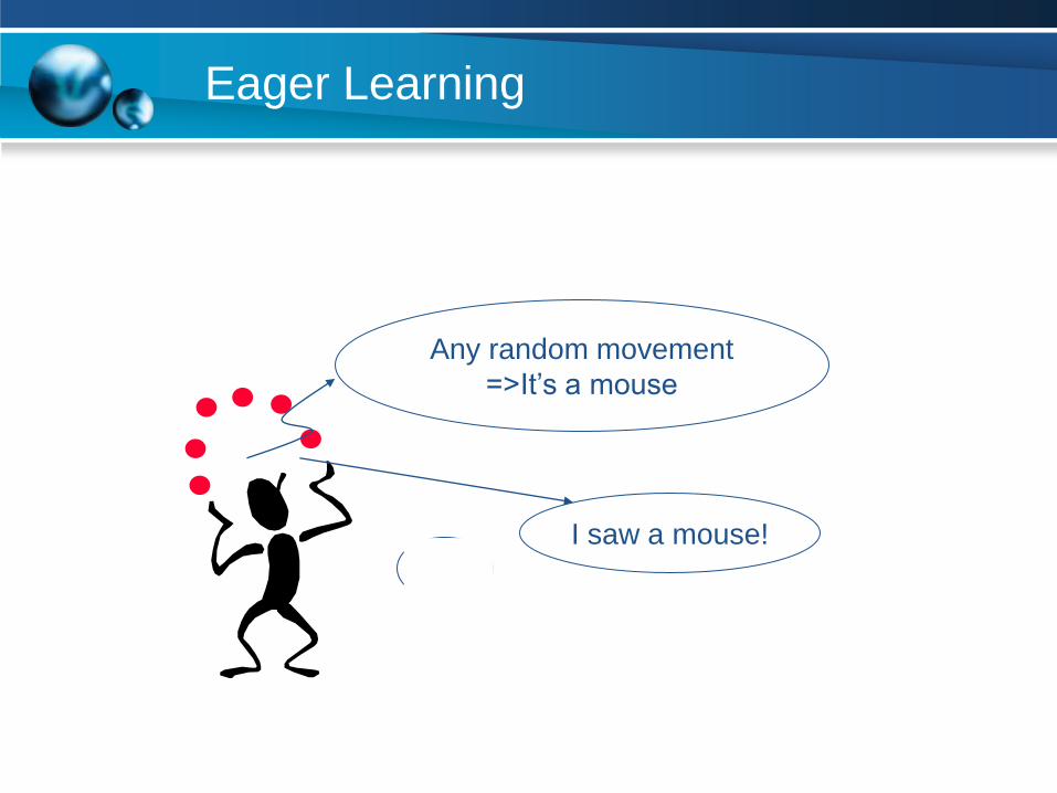
Any random movement

=>It’s a mouse

I saw a mouse!

Eager Learning

Its very similar to a

Desktop!!

Lazy Learning

Eager Learning

◘ Bir örneklemin sınıflandırılmasından önce, training set

verilerine göre sınıflandırma modelinin oluşturulması.

◘ Example models:

Decision tree Neural Network Support Vector Machine

Lazy Learning

◘ Sınıflandırılacak bir örneklem gelene kadar training verisi saklanır.

◘ Training süresi kısa fakat tahminleme/sınıflandırma süresi daha fazladır.

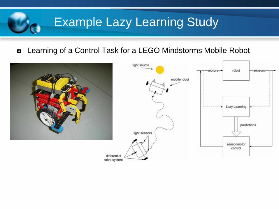
Example Lazy Learning Study

◘ Learning of a Control Task for a LEGO Mindstorms Mobile Robot

Lazy Learner: Instance-Based Methods

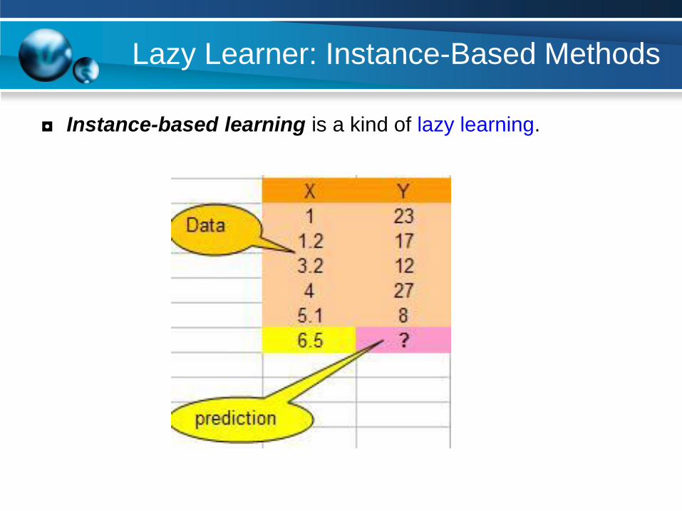
◘ Instance-based learning is a kind of lazy learning.

Instance Based Learning

◘ No model is learned

◘ The training instances which have been stored in memory

themselves represent the knowledge

◘ Training instances are searched for instance that most closely

resembles new instance

Instance Based Learning

Typical approaches

◘ k-Nearest Neighbor

◘ Weighted regression

◘ Case-based reasoning

k-Nearest Neighbor

k-Nearest Neighbor

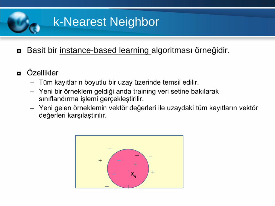
◘ Basit bir instance-based learning algoritması örneğidir.

◘ Özellikler

– Tüm kayıtlar n boyutlu bir uzay üzerinde temsil edilir.

– Yeni bir örneklem geldiği anda training veri setine bakılarak sınıflandırma işlemi gerçekleştirilir.

– Yeni gelen örneklemin vektör değerleri ile uzaydaki tüm kayıtların vektör değerleri karşılaştırılır.

.

_ +

_ xq

+

_ _ +

_

_

+

k-Nearest Neighbor Classification

◘ Sınıflandırmada (classification) kullanılan bu algoritmaya göre,

sınıflandırma sırasında çıkarılan özelliklerden (feature extraction),

sınıflandırılmak istenen yeni bireyin daha önceki bireylerden k

tanesine yakınlığına bakılmasıdır.

k-Nearest Neighbor

◘ Genelde real valued attributeleri destekler.

◘ Genelde Euclidean distance formülü kullanılır.

◘ Örneklemin sınıfı, kendisine en yakın k komşunun sahip olmuş olduğu çoğunluk sınıfıdır.

where (x,y) = 1 if x = y, else 0.

dist(x,y) (xi yi)2

i1

m

f^

(xq ) argmaxvV

(v, f (x i))i1

k

k-Nearest Neighbor

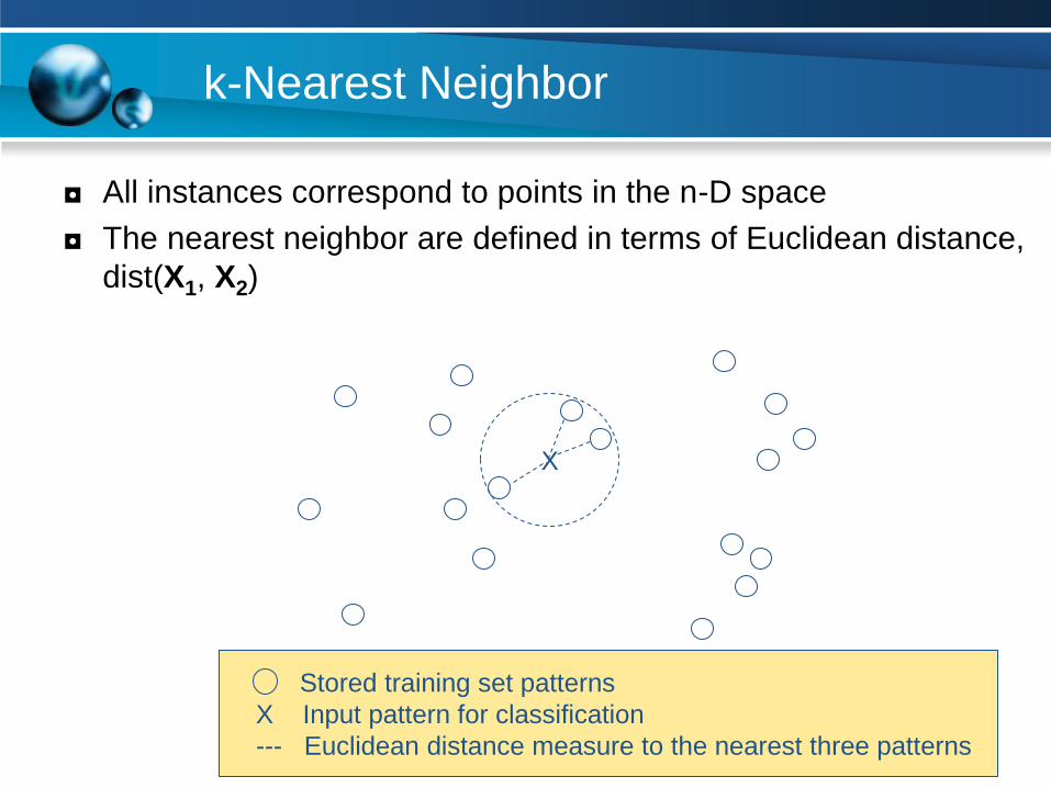
◘ All instances correspond to points in the n-D space

◘ The nearest neighbor are defined in terms of Euclidean distance,

dist(X1, X2)

X

Stored training set patterns

X Input pattern for classification

--- Euclidean distance measure to the nearest three patterns

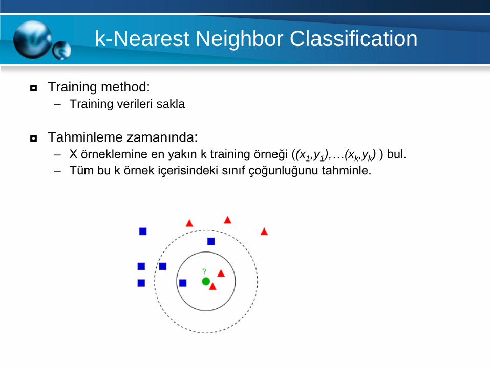
k-Nearest Neighbor Classification

◘ Training method:

– Training verileri sakla

◘ Tahminleme zamanında:

– X örneklemine en yakın k training örneği ((x1,y1),…(xk,yk) ) bul.

– Tüm bu k örnek içerisindeki sınıf çoğunluğunu tahminle.

Example Application

Document Classification (k=6)

Government

Science

Arts

P(science| )?

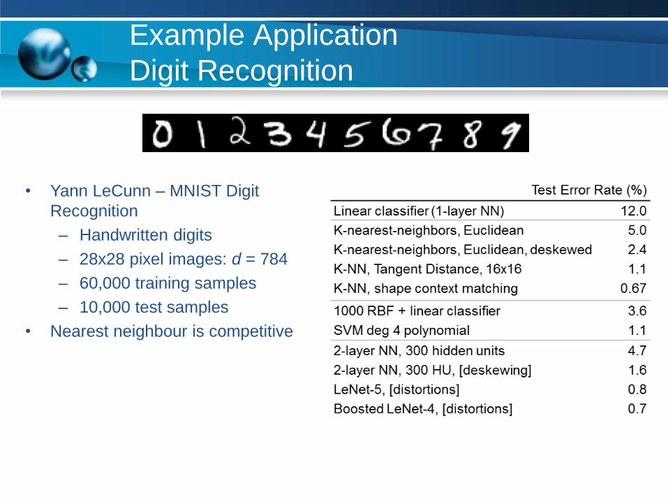
Example Application

Digit Recognition

• Yann LeCunn – MNIST Digit

Recognition

– Handwritten digits

– 28x28 pixel images: d = 784

– 60,000 training samples

– 10,000 test samples

• Nearest neighbour is competitive

Distance Formula

◘ Euclidian distance: square root of sum of squares of differences for two features: (x)2 + (y)2

◘ Intuition: similar samples should be close to each other

5-nearest neighbors:

q1 is classified as negative

+ +

+ +

-

- -

-

-

- q1

Other Distance Measures

◘ City-block distance (Manhattan dist)

◘ Cosine similarity

◘ Jaccard distance

◘ Others

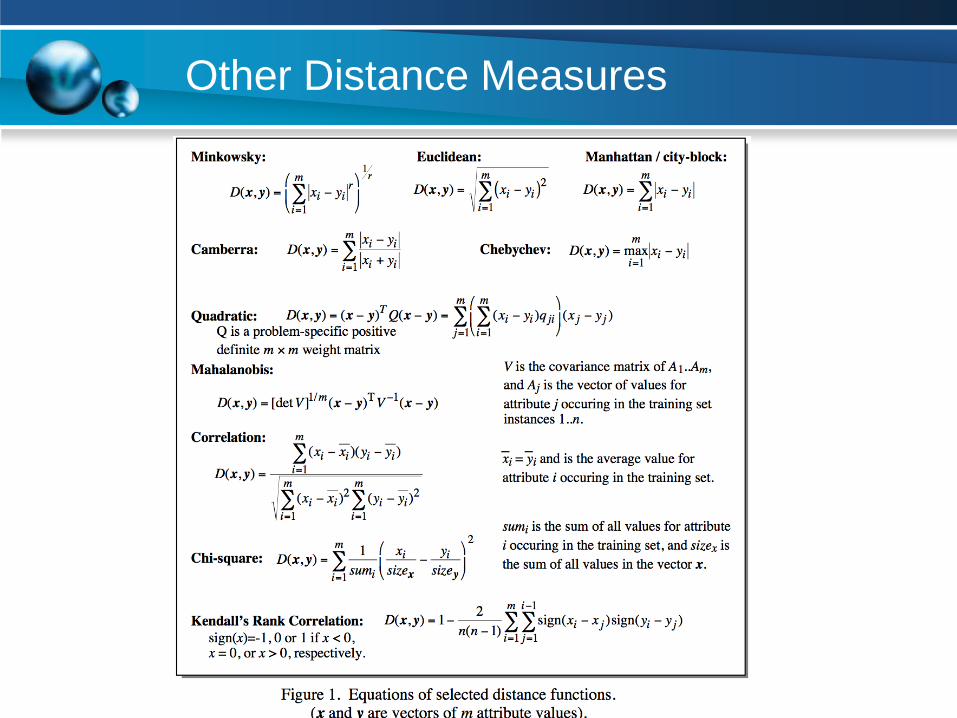
Other Distance Measures

Non-Numeric Data

◘ Peki özellik değerleri sayısal değilse?

◘ Example

– Boolean values: Yes or no, presence or absence of an attribute

– Categories: Colors, educational attainment, gender

◘ Uzaklık nasıl hesaplanacak?

Dealing with Non-Numeric Data

◘ If the attribute a is discrete, then :

◘ Boolean values => convert to 0 or 1

– Applies to yes-no/presence-absence attributes

◘ Non-binary characterizations

– Use natural progression when applicable; e.g., educational attainment: GS, HS, College, MS, PHD => 1,2,3,4,5

– Assign arbitrary numbers but be careful about distances; e.g., color: red, yellow, blue => 1,2,3

◘ How about unavailable data? (0 value not always the answer)

otherwise.1,

)a()a( if0, jijia

xx),x(xd

Examples

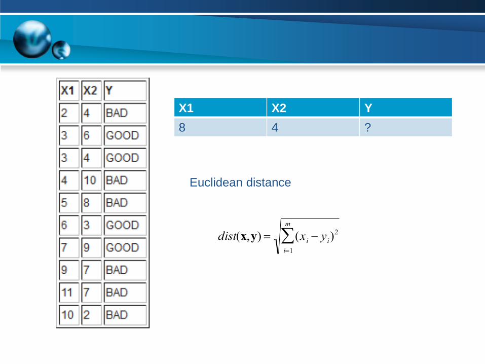
X1 X2 Y

8 4 ?

dist(x,y) (xi yi)2

i1

m

Euclidean distance

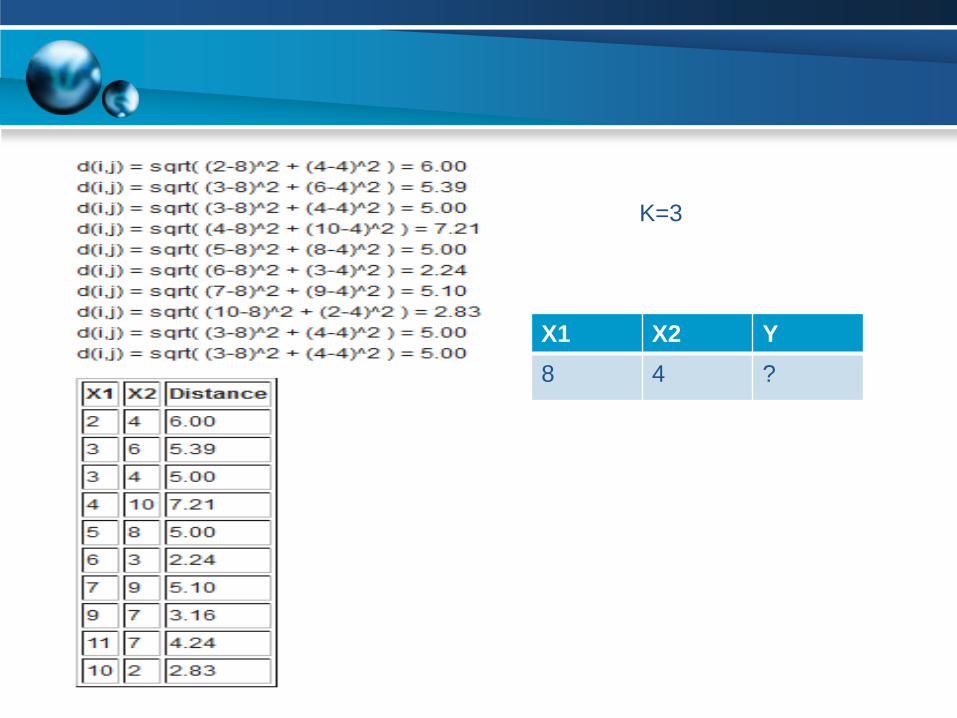
X1 X2 Y

8 4 ?

K=3

X1 X2 Y

6 3 GOOD

10 2 BAD

9 7 BAD

K=3

X1 X2 Y

8 4 BAD

New instance

Discussion on k-NN

k-NN Time Complexity

◘ Suppose there are m instances and n features in the dataset

◘ Nearest neighbor algorithm requires computing m distances

◘ Each distance computation involves scanning through each

feature value

◘ Running time complexity is proportional to m X n

Advantages

◘ Learning is very simple (fast learning)

◘ Robust to noisy data by averaging k-nearest neighbors

◘ Scales well with large number of classes

◘ In most cases it’s more accurate than NB or Rocchio

◘ Easy to understand which facilitates implementation and

modification.

Disadvantages

◘ Classification is time consuming

◘ Have to calculate the distance of the test case from all training

cases

◘ Memory intensive: require significant storage

◘ The accuracy of the algorithm degrades with increase of

irrelevant attributes.