institutions, credit rationing and housing development

Institutions, Credit rationing and housing development Fernanda Brollo and Fernando Garcia São Paulo School of Economics, Getulio Vargas Foundation, Brazil

Abstract

One of the basic principles that allow a smooth operation of the markets is the equilib-rium between supply and demand. According to this principle, when demand exceeds supply, the price mechanism will try to bring the system back into equilibrium. When this thinking is applied to the housing market, it leads to the conclusion that any inequality in housing supply or demand is transitory. Nonetheless, the fact that a considerable share of the population live in precarious homes for generations seems to speak against the virtues of market mechanisms in the resolution of housing disequilibria. Stiglitz and Weiss (1981) argue that in the face of asymmetric information, under some conditions the equilibrium of the credit market can be marked by rationing. Asymmetric information – working through the effects of adverse selection and of incentive – has im-pacts on the return function of bank loans, which leads to interest rates used in housing loans to be different from those that balance supply and demand for credit, causing credit rationing. Literature of the New Institutional Economics (NIE) in turn points out the fact that institutions can reduce the degree of uncertainty by lessening the effects of asymmet-ric information. Regarding the housing market, the degree of property rights, as well as the mortgage institution which acts as a contract enforcement tool, provide the credit market with information on the quality of the borrower and thus broaden the social scope of this market. The purpose of this article is to understand how the equilibrium in the housing market is influenced by credit rationing and to what extend institutional devel-opment affects this scarcity and the interest rates of housing loans. The model developed in this article, which combines the tradition of dynamic models of housing investment with the premises of the New Institutional Economics and the considerations of Stiglitz and Weiss (1981) and (1992) on rationing in the credit market, allows us to identify the role of institutions on housing development.

Key-words: Property rights, Mortgage foreclosure costs, Asymmetric information, Rationed credit market, Housing development

JEL Code: R21, R31, G21, D23

1

1. Introduction

One of the basic principles that allow a smooth operation of markets is the equi-librium between supply and demand. According to this principle, when demand exceeds supply, the price mechanism brings the system back into equilibrium, re-ducing demand or increasing supply until a balance is reached where no shortage of goods is found. The lack and surplus of goods in market are, within this context, transitory situations that temporally bind two stable equilibriums. When this thinking is applied to the housing market, it leads to the conclu-sion that any inequality in housing supply or demand is also transitory. A possible excess of demand caused, say, by a demographic boom or by a large migration flow would raise housing prices in a given region, i.e., leading to higher rents. These higher prices would in turn trigger new investment, considering that at a given interest rate, the yield of real estate investment would be more attractive than that of other investment alternatives. In the case of a family renting a home, higher rent in comparison to the interest rate would signal that this would be a good time to seek a mortgage. In the case of a family with savings, this higher rent would tell them that this would be the right moment to use their assets invested in other ways to buy a home. In either case, a shortage of homes in the market would lead, through higher prices, to greater real estate investment, with a simul-taneous growth of both demand and supply of credit in financial market. The price mechanism in housing markets was first formalized in Muth (1960), later improved on by Muth and Goodman (1989), summarizing the hous-ing-market analysis in the partial equilibrium tradition. By admitting the exis-tence of an homogeneous housing stock, the capacity to generate housing services became an increasing function of the capital stock. Following this tradition, the financial market supplies all the necessary capital for investment in the housing market, a fact which renders any disequilibria transitory. The same argument of investment behavior was established in a dynamic context by Tobin (1969). Considering the case of housing market, Tobin’s q can be defined as the ratio between housing market price and the cost of replacing a housing capital unit. This relative price would signal the real estate market, which price would also reflect the net return of housing investments. In this ap-

2

proach, real estate appreciation is given by the difference in current price and ex-pected value of housing capital, less its depreciation, plus the rent owned. The equilibrium condition in the financial market, which presupposes the existence of arbitrage, imposes the equality between the return on investment and the market interest rate. Any excess demand for housing services would appreciate real state market price relatively to the cost of replacing a housing capital unit, leaving Tobin’s q higher than 1, which induces investments. At the long term, housing capital accumulation would increase the supply of housing services clearing this market. The excess demand lasts only for the time necessary for the planning and building of new homes.1 One aspect in common in all these approaches is the perfect credit market premise, which provides all the necessary capital to carry out the desired real es-tate investments. Nonetheless, if the capital market does not supply the necessary capital for carrying out the desired real estate investments, the rise in rent prices caused by an excess demand will not necessarily subside. Consequently, there will be other factors affecting the equilibrium in the real estate market. In particular, if the housing credit market is rationed, for any reason whatsoever, the adjust-ment dynamics can be different from that analyzed by the approaches above de-scribed. In addition, the fact that a considerable share of the population, particu-larly in less-developed nations, has lived in precarious homes for generations ap-parently speaks against the virtues of market mechanisms in the resolution of housing disequilibria. We use the word “apparently”, because in most of these na-tions, it must be said, both the real state market as well as the credit market are not necessarily of the sort that ensures stable dynamic equilibriums without ra-tioning. The line of thinking described above assumes a series of conditions to achieve this, which are not necessarily fulfilled in developed countries and mainly in developing nations: (i) property rights must be secured; (ii) legal safeguards must ensure the binding of contracts; (iii) both the rent and the interest rate must be freely set by the parties; and (iv) there must be only one financial market, which efficiently allocates savings.

1 Following the tradition of rational expectations, Sheffrin (1983) sums up the previous argu-ments and formalizes a dynamic model of housing, in which appreciation of housing prices, inflation, and taxes drive housing investments.

3

Obviously, if one or more of these conditions is not fully satisfied, the mar-ket mechanisms will lose their equilibrium-seeking characteristics and the rela-tive scarcity will not be addressed automatically along time. This happens because in a market in which these conditions are not present, the return on investments will be surrounded by uncertainty and real estate credit could be rationed. Stiglitz and Weiss (1981) argue that in the presence of asymmetric infor-mation, the equilibrium of the credit market can be rationed, in the sense that, among apparently identical credit applicants, some are able to secure credit and others not, or there are some particular groups of individuals in society that are redlined from the credit market. This happens because when banks provide credit, they try to maximize their return by focusing on the following two aspects: the cost of loanable funds, and the risk involved in the project undertaken. According this authors, because the imperfect market information, the terms of credit con-tracts – the need for collateral and the interest rate set by the bank – as well as the amount of the loan can indeed affect the quality of the group of borrowers in two ways: (i) the adverse selection effect of borrowers2; and (ii) the incentive effect3. This article analyzes the real estate market, emphasizing the role of credit in long-term adjustment. It goes on to evaluate how asymmetric information and the absence of liquidity mechanisms, the result of the lack of the four conditions described above can end up rationing real estate credit. Finally, it suggests a ra-tioned-credit model for housing market, in which the short-term interest rate, credit availability and institutional development play a fundamental role in the equilibrium of the housing market.

2 By dissuading “safe” investors, i.e., those who invest in less risky projects, from seeking loans in banks, the contract can change the distribution of the group of borrowers. Considering that the bank’s expected return depends on the probability of those loans being repaid, borrowers who are aware of the scant probability of paying back their loans and are willing to pay higher interest rates will automatically be considered low-quality borrowers. Likewise, inasmuch as higher guarantee demands reduce the average degree of risk-aversion of the group of borrow-ers, the banks’ return is also reduced. 3 The incentive effect reflects changes in the behavior of investors, who prefer higher-risk pro-jects. Adjustments in the prime interest rate (which is also a part of the loan’s cost) and in the terms of the contracts {C, r} affect the behavior of the borrower: with a higher prime interest rate, we see a reduction in the expected return for the investor of the project to be financed, which leads such investor to seek higher-risk projects. These are projects with slim chances of success, but if successful can bring substantial returns.

4

2. Rationing in credit market: the general argument

Following Stiglitz and Weiss (1981), in a market with imperfect information, banks do not know how to screen the individual borrower, because they are not able to directly control the actions of all borrowers4. Thus, loan contracts are drafted so as to induce borrowers to take actions that are of interest to the bank and to lure high-quality borrowers, with low-risk projects. One of the mechanisms that help sort out “good” and “bad” borrowers is the loan’s interest rate. For a given interest rate, the expected profits of the firm increase with the risk of the project. To see if the interest rate acts as a protection mechanism for banks, the following is set by the authors: for a given loan interest rate ( r ), there is a critical value of risky project θ for which the agent borrows from the bank, if and only if

θθ ˆ> . Supposing that all loans have the same amount, the net return for the bor-rower is described by equation (1). In this equation, the investor’s expected return is the higher of the following values: (i) the level of wealth (W), plus the return of the project (R), less the amount of the loan, interests included (B + r.B); or (ii) the level of wealth, less the amount of the collaterals required by the credit contract (C). The first value holds if project is successful, otherwise holds the second value. Therefore, the value of θ for which the agent’s expected return is zero must sat-isfy the following condition:

(1) [ ]∏ ∫∞

=θ−+−+≡θ0

0),(;)1(max),( RdFCWBrRWr ,

where i is the prime interest rate, W0 is the initial level of wealth, C0 denotes the present value of collateral C. Therefore, )1(0 iWW += and ).1(0 iCC +=

Analyzing the credit supply side, the banks’ expected return on a loan, be-cause of the adverse selection effect, is a decreasing function of the risk degree of the loan and is given by expression (2). According to this equation, the borrower must pay to the bank the total amount of the debt or the most he can pay if the project failures, (R + C).

4 In this paper, we consider only loans supplied by the formal credit market. An extension of this argument to an economy with informal credit market, in which social norms are the true mechanism of contract enforcement, could be seen in Ghosh, Mookherjee and Ray (2000).

5

(2) ))1(;min(),( rBCRrR ++=ρ

The adverse selection argument, in which higher interest rates can lead to falling bank returns, comes from the fact that on average the quality of the bor-rowers deteriorates; i.e., the higher the interest rates, the greater the value of θ . This result is obtained when equation (1) is differentiated:

0ˆ/

)ˆ,(ˆ )1( >θ∂∏∂

θ=

θ ∫∞

−+ CBrRdFB

drd

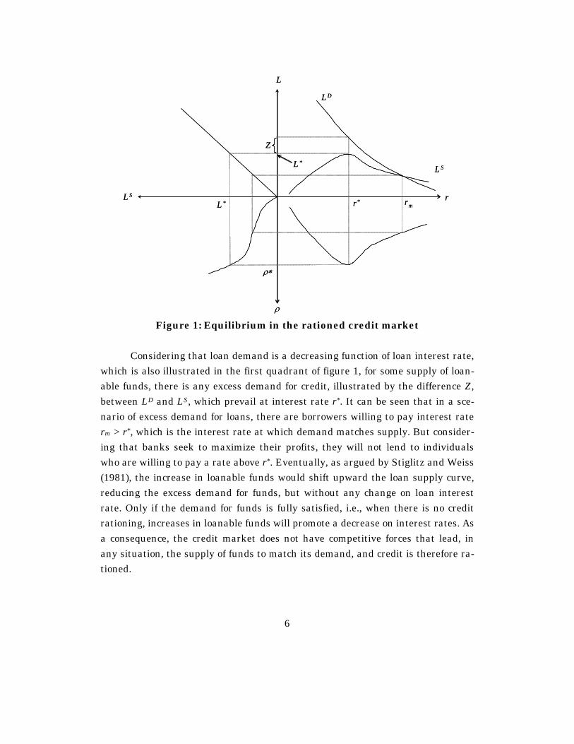
The second way in which the interest rate affects the banks’ expected re-turn on granted loans is the change in borrower behavior: as climbing interest rates raise the attractiveness of high-risk projects, the banks’ return is dimin-ished. Therefore, with an increase of r, the expected return of a project with a high chance of liquidation falls less than the expected return of a project with a smaller chance of liquidation. If a risk-neutral investor feels indifferently before two pro-jects, a rise in the interest rate will lead the agent to choose the project with a smaller chance of liquidating the loan. From this argument follows the main proposition about the relation be-tween loan interest rate and the expected return of banks. According to this proposition, ρ(r) will not be a monotonic function of r, which implies that there will be a ρ*, associated to r*, that maximizes expected returns of banks. Since is sup-posed that loans supply is an increasing monotonic function of the expected return of banks, there will be a level L* of loans supply that maximizes banks profits. Figure 1 illustrates how the credit market works when the interest rate is used as a shield against the incentive effect and the adverse selection effect that can re-duce the banks’ expected return.

In figure 1, the third quadrant shows the banks’ credit supply in relation to the expected return: the higher the loan’s expected return, the greater the credit offered. However, as shown in the second quadrant, the banks’ expected return increases at decreasing rates in relation to the interest rate. Therefore, there is an optimal rate of interest r*, that maximizes the banks’ expected return, above which this return starts to decrease. At equilibrium interest rate r*, which maxi-mizes the banks’ expected return, they supply L*. Any loan interest rate increase above r* would also reduce loan supply.

6

L

Z

LS

LD

r* rm

ρ

rLS

L*

ρ∗

L*

L

Z

LS

LD

r* rm

ρ

rLS

L*

ρ∗

L*

Figure 1: Equilibrium in the rationed credit market

Considering that loan demand is a decreasing function of loan interest rate,

which is also illustrated in the first quadrant of figure 1, for some supply of loan-able funds, there is any excess demand for credit, illustrated by the difference Z, between LD and LS, which prevail at interest rate r*. It can be seen that in a sce-nario of excess demand for loans, there are borrowers willing to pay interest rate rm > r*, which is the interest rate at which demand matches supply. But consider-ing that banks seek to maximize their profits, they will not lend to individuals who are willing to pay a rate above r*. Eventually, as argued by Stiglitz and Weiss (1981), the increase in loanable funds would shift upward the loan supply curve, reducing the excess demand for funds, but without any change on loan interest rate. Only if the demand for funds is fully satisfied, i.e., when there is no credit rationing, increases in loanable funds will promote a decrease on interest rates. As a consequence, the credit market does not have competitive forces that lead, in any situation, the supply of funds to match its demand, and credit is therefore ra-tioned.

7

However, according to Stiglitz and Weiss (1981), the interest rate is not the only contract factor that matters. The amount of the loan and its collaterals also affect the borrowers’ behavior. If banks demand higher guarantees, this can lead to borrowers willing to bear smaller risks, in less risky projects. On the other hand, demand for higher collateral can lead to a reduction in the banks’ return: if there is total aversion to decreasing risk, and if all individuals (with identical util-ity functions) face the same investment opportunities, wealthier individuals will be more willing to offer more collateral, which illustrates their disposition to em-bark on riskier projects than are less wealthy individuals. The effect of this ad-verse selection can dominate the positive effects of collateral requirement. As a consequence, there is also a limit after which it is no longer lucrative for banks to raise the requirement for guarantees in the presence of excess demand for credit, just as it happens with the loan’s interest rate.

Thus, the rationing of the credit market takes place if the following three conditions are met: (i) there is imperfect information; (ii) the effects of adverse se-lection and incentive are considerable; and (iii) the banks’ expected return under the Walrasian equilibrium must be lower than in any other contract with credit rationing. In Stiglitz and Weiss (1992) this analysis is expanded for the case in which both problems – incentive and adverse selection – are present. In this model, the banks use the required guarantees and the interest rates as instru-ments to screen and encourage borrowers. One of findings of this work is that the whole class of loan applicants can be rationed and that this rationing must take place with every contract.

3. The rationed credit market for real estate projects

Based on the Stiglitz and Weiss (1981) and (1992) rationing model, it is possible to describe a market for lending to real estate projects, with minor changes. Let’s initially consider that information is imperfect, that is, banks do not know how to screen the individual borrower credit risk. Therefore, the loan interest rate and the mortgage requirements end up being the mechanisms that reduce the effects of adverse selection and incentive. Equation (3) expresses the optimal loan interest rate, which is set up in order to maximize bank’s expected returns. In the same way, we can define the amount of credit supplied by banks,

8

L*, as a monotonic function of r* and of the amount of loanable funds in real estate market (S).

(3) )),((max* rRr ρ≡ ρ

(4) 0 and 0),,( *** >′>′≡ SrSrL lll

Note that the banks’ profits are defined as the difference between r* and loan costs, which are determined by the economy’s prime interest rate, the oppor-tunity costs, and the costs relative to safeguarding the property rights, incurred, say, in evaluating the value of the real estate property and in foreclosing mort-gages. In this sense, we say that operational costs associated with the degree of institutional development are included in banks spread.5

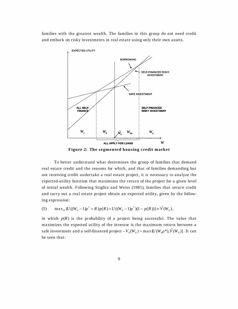
The credit demand for real estate projects satisfies three basic premises: (i) it is segmented into four different levels of wealth6 – Wc, Wb, Wba e Wa, such as Wc < Wb < Wba < Wa; (ii) wealth is comprised real assets, which can be used as col-laterals C, being that Cc < Cb < Cba < Ca, and of human capital income, from likely inheritance and retirement, H; and (iii) there is a minimum initial wealth level (Wi0 > C) to allow family i to be included in the group demanding housing credit, which will have its projects reviewed by the banks.

Figure (2) illustrates agent’s behavior in this market. Each individual has a safe investment alternative with return ρ*, with expected utility Ui(Wi0,r*). Fami-lies belonging to the c group are not part of the credit demand because they do not possess the minimum wealth requirement (Wc0 < C). For these families, both the expected utility of investing in a safe investment as well as that of a self-financed housing investment are greater than the expected utility of taking out a loan to undertake7 a real estate project. Families with wealth between Wb and Wa de-mand credit, because the expected utility for taking out a loan at the bank is greater than the risk-free investment. However, a subset of families, those which have wealth located in the Wba interval, will still undertake a project, even if they do not qualify for a loan, because the expected utility from these loans is above that of other investment alternatives. Lastly, the group Wa represents the set of

5 By construction, these costs are a nonmonotonic function of institutional development. 6 According to Stiglitz (1981) it is supposed that all borrowers are risk-averse with the same utility function U(W), U’ > 0, U” < 0 and that individuals differ only when it comes to wealth. 7 Housing investment with self-financing, for low-income families, can be seen as self-building.

9

families with the greatest wealth. The families in this group do not need credit and embark on risky investments in real estate using only their own assets.

ALL APPLY FOR LOANS

ALL SELF-FINANCE

SELF-FINANCED RISKY INVESTMENT

EXPECTED UTILITY

W


SAFE INVESTMENT

BORROWING

WbWc Wba WabW

ALL APPLY FOR LOANS

ALL SELF-FINANCE


EXPECTED UTILITY

W


SAFE INVESTMENT

BORROWING

WbWc Wba WabW

Figure 2: The segmented housing credit market

To better understand what determines the group of families that demand

real estate credit and the reasons for which, and that of families demanding but not receiving credit undertake a real estate project, it is necessary to analyze the expected-utility function that maximizes the return of the project for a given level of initial wealth. Following Stiglitz and Weiss (1981), families that secure credit and carry out a real estate project obtain an expected utility, given by the follow-ing expression:

(5) )(ˆ))}(1)()1(()())1(({max 0*

0*

0 WVRpWURpRWUR ≡−ρ−++ρ− ,

in which p(R) is the probability of a project being successful. The value that maximizes the expected utility of the investor is the maximum return between a safe investment and a self-financed project – )](ˆ*),(max{)( 0000 WVWUWV ρ= . It can be seen that:

10

**)(0

0 ρ′=ρ U

dWWdU and *)]1([)(ˆ

210

0 ρ−′+′= pUpUdW

WVd .

It can thus be established that risk aversion is absolutely decreasing; the greater the family’s initial level of wealth, the lesser the expected utility of the safe investment in relation to the investment in a risky project with self-financing, since:

0

0

0

0 )(ˆ*)(dW

WVddW

WdU<

ρ .

Therefore, there is a critical value of wealth Wb, such as, if the wealth is greater than this value, families not able to secure credit still embark on the real estate project – these are families in the interval Wba. For families with absolute and decreasing risk aversion and wealth below this critical value, the expected utility is give by equation (6):

(6) )()1)()(())ˆ1((max{ 0*

0*

0 WVpCWUpRrWU BR≡−ρ−+++−ρ .

In this case, individuals take out loans if, and only if, )()( 000 WVWVB ≥ . But since *

21 ))1((/ ρ−′+′= pUpUdWdVB , only when Wi0 > C, it is profitable to take out a loan. It is assumed that there is wealth different from zero, called Wb, such as Vb(Wb) = U(ρ*,Wb) – which is true for some values of ρ*. Using the same argument above, it becomes clear that in Wb the act of taking out a loan ensures medium utility that preserves the spread of terminal wealth in comparison with not taking out the loan and not embarking on the project. Therefore, if

0000 /)(/ dWWdVdWdVB > ,

for bb WWW ˆ0 << , all individuals qualify to take out a loan. Considering that

bWW ˆ0 < , if there is a loan, the wealthiest individual will be the one benefited8.

It is time now to analyze the effects of changes in exogenous variables on the housing credit market. Particular attention is given to the effects on equilib-rium in regards to: (a) institutional changes that lead to a reduction in the mort-gage transaction costs; (b) changes in monetary policy that imply in varying the

8 This restriction is weaker than the imposition of a scale of projects that exceeds the wealth of any individual.

11

cost of opportunity of loans or of loanable funds; (c) policies for the granting of subsidies; and (d) policies that secure property rights.

(a) The effects of a reduction in the mortgage transaction costs

The cost of foreclosing mortgages is one of the components of the banks’ to-tal loan cost that is intimately associated to the legal structure and to law en-forcement. In supposing a reduction is such costs – brought, say, by the creation of a real estate fiduciary ownership title – the banks’ total loan cost is thus reduced and, when passed on to the loan’s interest rate, changes the equilibrium of the rationed credit market. The effect of the reduction in the cost of foreclosing real guarantees on the demand and offer of credit is shown in figure (3).

ALL APPLY FOR LOANS

ALL SELF-FINANCE


EXPECTED UTILITY

W


SAFE INVESTMENT

BORROWING

WbWc Wab WabW

L

LS

LD

r*

ρ

rLS r**

ALL APPLY FOR LOANS

ALL SELF-FINANCE


EXPECTED UTILITY

W


SAFE INVESTMENT

BORROWING

WbWc Wab WabW

L

LS

LD

r*

ρ

rLS r**

L

LS

LD

r*

ρ

rLS r**

(a) (b)

Figure 3: The reduction in the cost of foreclosing mortgages The reduction in the loan’s interest rate gives the investor’s expected-utility

function in relation to his initial wealth (W0) a steeper slope. This means that equality between the expected return of the safe investment and that of borrowing assets and embarking on the real estate project becomes true for a lower level of initial wealth. This means that the number of families that seek credit rises, for a given wealth distribution. The result on the credit supply of loanable funds is shown in figure (3.b). In the graph’s second quadrant, we see the curve that re-lates the loan’s interest rate and the banks’ expected return shift downwards and

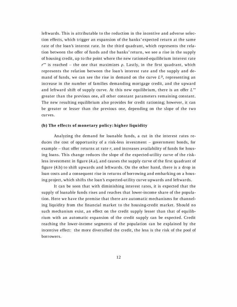
12

leftwards. This is attributable to the reduction in the incentive and adverse selec-tion effects, which trigger an expansion of the banks’ expected return at the same rate of the loan’s interest rate. In the third quadrant, which represents the rela-tion between the offer of funds and the banks’ return, we see a rise in the supply of housing credit, up to the point where the new rationed-equilibrium interest rate r** is reached – the one that maximizes ρ. Lastly, in the first quadrant, which represents the relation between the loan’s interest rate and the supply and de-mand of funds, we can see the rise in demand on the curve LD, representing an increase in the number of families demanding mortgage credit, and the upward and leftward shift of supply curve. At this new equilibrium, there is an offer L** greater than the previous one, all other constant parameters remaining constant. The new resulting equilibrium also provides for credit rationing; however, it can be greater or lesser than the previous one, depending on the slope of the two curves.

(b) The effects of monetary policy: higher liquidity

Analyzing the demand for loanable funds, a cut in the interest rates re-duces the cost of opportunity of a risk-less investment – government bonds, for example – that offer returns at rate r, and increases availability of funds for hous-ing loans. This change reduces the slope of the expected-utility curve of the risk-less investment in figure (4.a), and causes the supply curve of the first quadrant of figure (4.b) to shift upwards and leftwards. On the other hand, there is a drop in loan costs and a consequent rise in returns of borrowing and embarking on a hous-ing project, which shifts the loan’s expected-utility curve upwards and leftwards. It can be seen that with diminishing interest rates, it is expected that the supply of loanable funds rises and reaches that lower-income share of the popula-tion. Here we have the premise that there are automatic mechanisms for channel-ing liquidity from the financial market to the housing-credit market. Should no such mechanism exist, an effect on the credit supply lesser than that of equilib-rium with an automatic expansion of the credit supply can be expected. Credit reaching the lower-income segments of the population can be explained by the incentive effect: the more diversified the credit, the less is the risk of the pool of borrowers.

13

L

LS

LD

r*

ρ

rLS r**

W

WbWc Wab WabW

EXPECTED UTILITYBORROWING


SAFE INVESTMENT


ALL APPLY FOR LOANS

ALL SELF-FINANCE

L

LS

LD

r*

ρ

rLS r**

L

LS

LD

r*

ρ

rLS r**

W

WbWc Wab WabW

EXPECTED UTILITYBORROWING


SAFE INVESTMENT


ALL APPLY FOR LOANS

ALL SELF-FINANCE

(a) (b)

Figure 4: Higher liquidity in the credit market

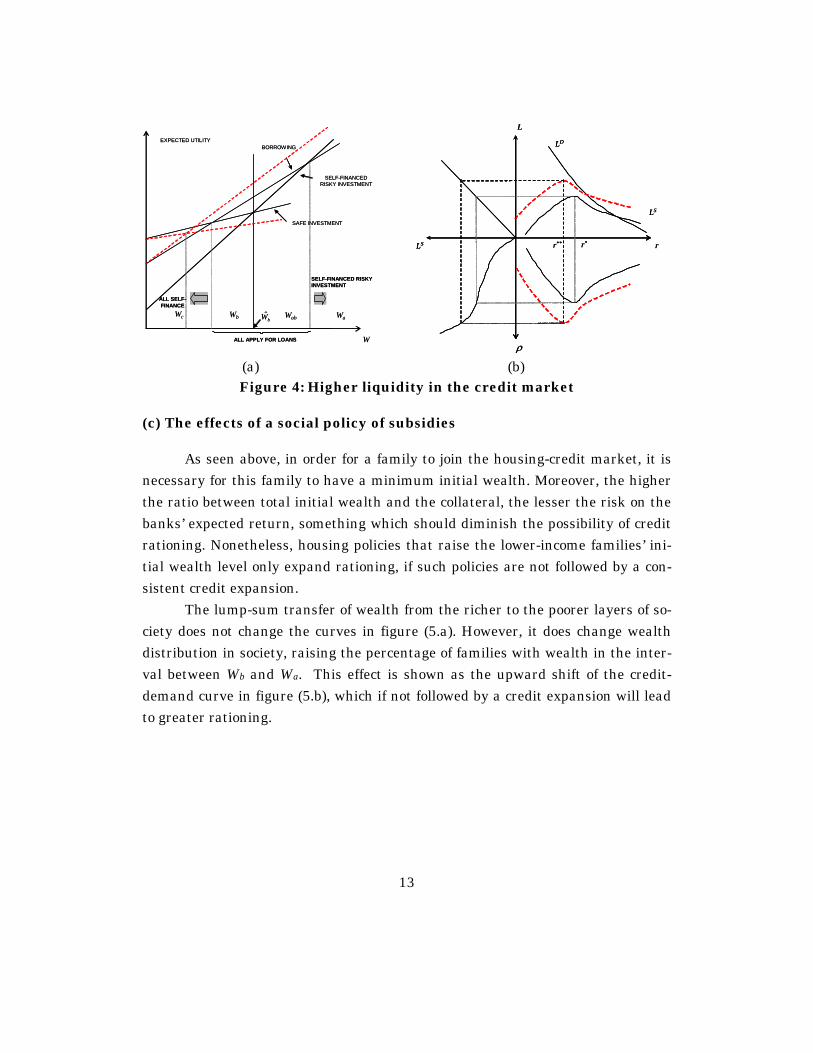
(c) The effects of a social policy of subsidies

As seen above, in order for a family to join the housing-credit market, it is necessary for this family to have a minimum initial wealth. Moreover, the higher the ratio between total initial wealth and the collateral, the lesser the risk on the banks’ expected return, something which should diminish the possibility of credit rationing. Nonetheless, housing policies that raise the lower-income families’ ini-tial wealth level only expand rationing, if such policies are not followed by a con-sistent credit expansion. The lump-sum transfer of wealth from the richer to the poorer layers of so-ciety does not change the curves in figure (5.a). However, it does change wealth distribution in society, raising the percentage of families with wealth in the inter-val between Wb and Wa. This effect is shown as the upward shift of the credit-demand curve in figure (5.b), which if not followed by a credit expansion will lead to greater rationing.

14

W

WbWc Wab Wa

L

LS

LD

r*

ρ

rLS r**

LD´

ALL APPLY FOR LOANS

ALL SELF-FINANCE


EXPECTED UTILITY


SAFE INVESTMENT

BORROWING

W

WbWc Wab Wa

L

LS

LD

r*

ρ

rLS r**

LD´

ALL APPLY FOR LOANS

ALL SELF-FINANCE


EXPECTED UTILITY


SAFE INVESTMENT

BORROWING

(a) (b)

Figure 5: The policy of subsidies

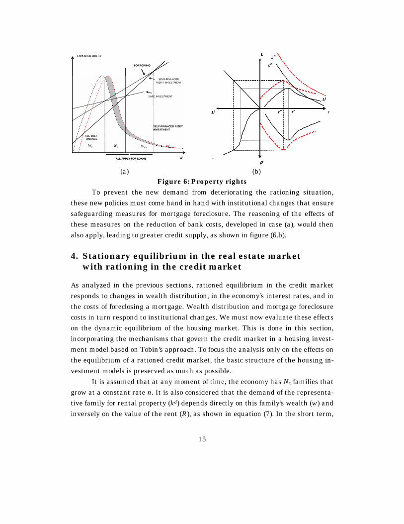
(d) The effects of securing property rights

To shed some light on the importance of secure property rights, and its re-lation with the development of a credit market, it might be worthwhile to quote De Soto (2000). The author argues that there are families in poor countries that hold substantial assets, but the lack of due property rights prevents these assets from being used as collateral for credit purposes, thus limiting the potential use of this property. In contrast, he cites the case of rich countries, where property rights are well defined and the full potential of assets is exploited. This means that within an environment where property rights are safeguarded, there would be room for a secondary market for mortgage securities. Raising the level of wealth of these families stokes the credit market, which in turn leads to housing development. Figure (6) shows the effects of securing property rights in the housing-credit market. Considering that property rights raise the wealth of the families, the curve of the families’ wealth is shifted right-wards, increasing the number of families demanding housing credit. However, in order to have a positive effect of these policies on the credit market, and conse-quent improvement of the housing development, it is not enough to secure prop-erty rights. If the credit offer remains unchanged, the result will be a higher ex-cess demand for credit.

15

W

WbWc Wab Wa

L

LS

r*

ρ

rLS r**

LD

LD´

ALL APPLY FOR LOANS

ALL SELF-FINANCE


EXPECTED UTILITY


SAFE INVESTMENT

BORROWING

W

WbWc Wab Wa

L

LS

r*

ρ

rLS r**

LD

LD´ L

LS

r*

ρ

rLS r**

LD

LD´

ALL APPLY FOR LOANS

ALL SELF-FINANCE


EXPECTED UTILITY


SAFE INVESTMENT

BORROWING

(a) (b)

Figure 6: Property rights To prevent the new demand from deteriorating the rationing situation, these new policies must come hand in hand with institutional changes that ensure safeguarding measures for mortgage foreclosure. The reasoning of the effects of these measures on the reduction of bank costs, developed in case (a), would then also apply, leading to greater credit supply, as shown in figure (6.b).

4. Stationary equilibrium in the real estate market with rationing in the credit market

As analyzed in the previous sections, rationed equilibrium in the credit market responds to changes in wealth distribution, in the economy’s interest rates, and in the costs of foreclosing a mortgage. Wealth distribution and mortgage foreclosure costs in turn respond to institutional changes. We must now evaluate these effects on the dynamic equilibrium of the housing market. This is done in this section, incorporating the mechanisms that govern the credit market in a housing invest-ment model based on Tobin’s approach. To focus the analysis only on the effects on the equilibrium of a rationed credit market, the basic structure of the housing in-vestment models is preserved as much as possible. It is assumed that at any moment of time, the economy has Nt families that grow at a constant rate n. It is also considered that the demand of the representa-tive family for rental property (kd) depends directly on this family’s wealth (w) and inversely on the value of the rent (R), as shown in equation (7). In the short term,

16

the supply of real estate property is fixed – expression (8) – which implies that the rent rate is determined only by demand conditions, as stated in equation (9).

(7) 0and0,.)( >β>′β−= wttdt fRwfk

(8) ttst kkk == 0

(9) β

−= tt

tkwfR )(

Following Tobin (1969), tq is defined as the ratio between market price ( tp ) and the replacement cost of one unit of housing capital ( tc ) – equation (5.4). When

tq > 1, the market price of one housing unit is greater than the cost of building an identical housing unit. In this case, it is said that there is incentive to invest, more specifically in our case, in the building of new housing units. If tq < 1, conversely, it is cheaper to buy a ready home than to build one; in this case the families are not encouraged to invest in the building of homes.

(10) t

tt c

pq =

If we suppose that the construction cost is constant, tq becomes the relative real estate property’s market value, and it will vary according to tp fluctuations, which is determined by return, less depreciation, provided by rental income. For the rental sector, the return from one period to the next will be the ratio between the total amount available to the owner in the following period and the value of the property in the initial period. The total amount available to the owner in the subsequent period will be the following: the new market value of the property, plus rent income, less depreciation of the previous stock. For continuous time, equation (11) defines the investment’s rate of return:

(11) Returnt

ttt

qqRq δ−+

=&

Because capital market is not perfect – it can be affected by asymmetric information that leads to credit rationing – families are not able to fully arbitrage between gains in the rent market and those from the financial assets market. In fact, if the rent income, net of depreciation, is above the interest rate, families will

17

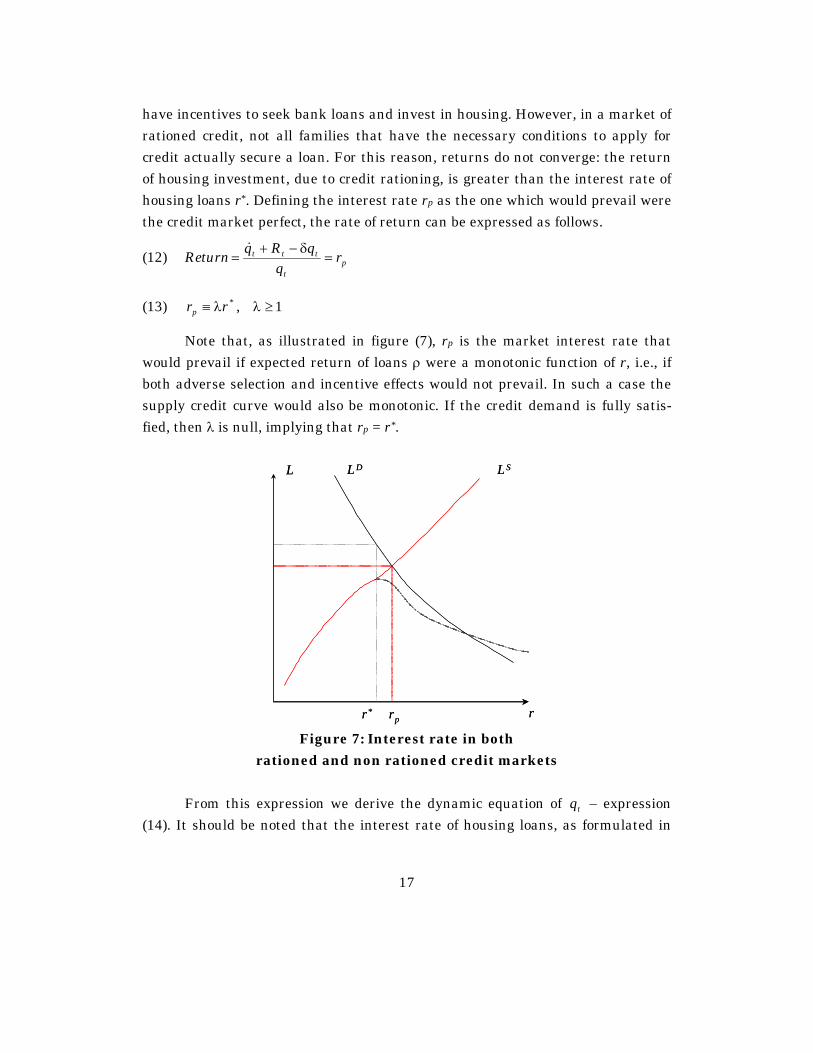
have incentives to seek bank loans and invest in housing. However, in a market of rationed credit, not all families that have the necessary conditions to apply for credit actually secure a loan. For this reason, returns do not converge: the return of housing investment, due to credit rationing, is greater than the interest rate of housing loans r*. Defining the interest rate rp as the one which would prevail were the credit market perfect, the rate of return can be expressed as follows.

(12) Return pt

ttt rq

qRq=

δ−+=&

(13) *rrp λ≡ , 1≥λ

Note that, as illustrated in figure (7), rp is the market interest rate that would prevail if expected return of loans ρ were a monotonic function of r, i.e., if both adverse selection and incentive effects would not prevail. In such a case the supply credit curve would also be monotonic. If the credit demand is fully satis-fied, then λ is null, implying that rp = r*.

L LSLD

r* rp r

L LSLD

r* rp r Figure 7: Interest rate in both

rationed and non rationed credit markets From this expression we derive the dynamic equation of tq – expression (14). It should be noted that the interest rate of housing loans, as formulated in

18

section 3, is a function of the market interest rate, of mortgage foreclosure costs, and of the other administrative costs, and is defined by the process in which banks maximize the return of their loans. Note that we assume a decreasing relation between the degree of institutional development, given by law enforcement and property rights, and the mortgage foreclosure costs. In this sense, less institution-ally developed economies will show greater loan rates in housing credit market.

(14) β

−−δ+λ=−δ+= tt

tttp

tkwfqrRqrq )().().( *&

(15) ttt knik )( δ+−=&

The accumulation of the housing capital per family is given by expression (15). What in essence changes is the investment function of the families. Here it is defined with the aggregation of investment performed by three wealth layers of society: a, b and c, such that Wc < Wb < Wa. We assume that all layers grow at a constant rate n. As already argued in section 3, there is a W0, which is the mini-mum critical wealth level that a family must have to belong to the rationed-credit market, such that Wc < W0 < Wb. The investment of families that belong to the a and c layers are self-financed, as described in section 3, and it depends only on the real estate market value, because they are supposed to be based on identical and homothetic preference structures. Equation (16) expresses this relation, where

1−=π tt q is the excess of real estate market price over unit construction costs, and 0>σ , showing that a greater real estate market value will stimulate invest-ments.

(16) tta

tc ii πσ≡≡ .

For the b layer of wealth, the investment function is defined by the sum of the financed investment, which is determined in the equilibrium of the credit market L*, with self-investment performed by those families that seek credit but do not receive it. Please note that L* is the financed value of the property, which can be expressed by the product of the number of contracts with the price of fi-nanced real estate. On behalf of simplicity, it is assumed that the self-investment share of this layer of wealth is identical to the investment function of the other wealth layers. Expression (17) shows this relation.

19

(17) ).(*ttt

bi πσ+≡ l

Loans per family )( tl in the rationed-credit market are given by equation (18), which establishes the basic relation discussed in the last section among the amount of loans, interest rate, mortgage foreclosure costs and loanable funds.

(18) ),( **ttt srg=l

In this equation, a reduction on the prime interest rate has positive impacts on the credit supply per family, so that 0<′rg . On the other hand, an expansion on loanable funds per family ( ts ) has a positive effect on credit supply, so that,

0>′sg . Thus, the investment per family is defined by expression (19). Substitut-ing this last expression in (20) we arrive at the equation of capital accumulation.

(19) )1.(),( * −σ+≡ tttt qsrgi

(20) ttttt knqsrgk ).()1.(),( * δ+−−σ+=&

Equations (14) and (20) form a system of differential equations with saddle stability, as showed in the Mathematical Appendix. Based on these equations, in the appendix we also derive the curves of stationary dynamics of tq and of tk , as well as the steady state equilibrium. This system is showed in figure 8.

tk

tq0kt =&

0qt =&

*q

*k Figure 8: Steady state equilibrium in housing market

20

Finally, it is worthwhile to point out the effects of institutional changes on the equilibrium of the housing market, which compete with changes in wealth distribution and monetary policy. These effects can be evaluated by the model’s comparative statics, which is calculated from the application of the implicit func-tion theorem in the system formed by equations (A.1) and (A.12), if all other pa-rameters remain constant.

dsg

dwf

drgq

dkdq

nr

s

w

tr

t ⋅

′−

+⋅

β

′+⋅

′−

λ−=

⋅

δ+−σβδ+λ 0

0)(1)( *

*

**

Propositions 1, 2 and 3 below bring the reaction of changes in the interest rate, in the economy’s average wealth, and in the availability of loanable funds in the equilibrium of the housing market. Proposition 1: A rise in prime interest rates depresses the price of real estate, but this it can have either positive or negative impacts on the steady-state stock of housing capital per family. This conclusion emerges directly from the derivates of q* and k* in relation to r*. The first derivate,

0))((

).(.(*

*

*

*

<δ+λδ+β+σσλ−δ+λ′β

=rn

qrgdrdq r ,

is negative, since the numerator is negative, unlike the denominator, which is positive. But the second derivate could have either positive or negative signal, since rg′ is a negative parameter:

))(())((

**

*

δ+λδ+β+σδ+βλ+′−

=rn

nqgdrdk r .

Proposition 2: The expansion of wealth raises market prices of real estate and leads to a greater stock of capital. This result comes from the derivates of q* and k* in relation to w, due to the positive effect of wealth on demand for housing services:

0))((

).(.*

*

>δ+λδ+β+σ

δ+′β=

rnnf

dwdq w and 0

))((..

*

*

>δ+λδ+β+σ

σ′β=

rnf

dwdk w .

21

Proposition 3: An increase in loanable funds brings a steady-state equilibrium with greater level of welfare, in which the housing capital per family is higher, and the price of real estate is lower. This argument is implied directly by the fact that an expansion on loanable funds has a positive impact on credit supply per family, as discussed in section 3.

0))(( *

*

<δ+λδ+β+σ

′−=

rng

dsdq S

t and 0

))(().(.

*

**

>δ+λδ+β+σ

δ+λβ′=

rnrg

dsdk S

t.

Therefore, the monetary policy that leads to a low prime interest rate, al-though leaves real estate investments more attractive, does not necessarily leads to an increase in the stock of housing capital, since rationing on real estate credit market can inhibit housing investments. In its turn, housing policies that drive more funds to credit market, as a consequence of developing an environment where property rights are safeguarded, i.e. improving the secondary market for mortgage securities, have unambiguous welfare effects, since they leads to low real estate property prices and high housing capital per family.

5. Concluding remarks

The model developed in this article, which combines the tradition of dynamic models of housing investment with the premises of the New Institutional Econom-ics and the considerations of Stiglitz and Weiss (1981) and (1992) on rationing in the credit market, allows us to identify the role of institutions on housing devel-opment. Economies that better ensure property rights, with the effects this has on wealth distribution in society, reach higher levels of housing development. This degree of property rights is intimately associated to the granting of property titles. In societies in which land is not properly held, this attribution is smaller, which in turn reduces the demand for credit and the role this market can play in housing development. On the other hand, institutions that ensure due fulfillment of contracts, such as legislation that allows automatic mortgage foreclosure, or a secondary market for mortgages, reduce the transaction costs and consequently the interest rate of real estate loans. This has a negative effect on credit rationing, which al-

22

lows banks to finance more families, with the consequent impact on housing de-velopment. The argument formalized in this paper corroborates the arguments of Barzel (1997) and De Soto (2000), among others, on the role of institutions and of property rights in economic development. Future research in this field should therefore seek to empirically identify if credit is rationed and if property rights affect the equilibrium price of housing loans. In this area, it is worthwhile to com-pare countries with developed credit markets and institutions with others in which neither institutions nor the financial market are developed.

References

Barzel, Y. (1997): Economic Analysis of Property Rights, Cambridge University Press.

De Soto, H. (2000): The mystery of capital: why capitalism triumphs in the West and fails everywhere else. Basic Books.

Ghosh, P., Mookherjee, D. and Ray, D. (2000): Credit Rationing in Developing Countries: An Overview of the Theory. In Mookherjee, D and Ray, D., A Reader in Development Economics, London: Blackwell (2000).

Muth, R.C. (1960): The Demand for Non-Farming Housing. In Harberger, A.C.: The Demand for Durable Goods. Chicago. The University of Chicago Press, 1960.

Muth, R.C. e Goodman, A.C. (1989): The Economics of Housing Markets. Har-wood Academic Publishers.

Sheffrin, S. (1983): Rational Expectations. Cambridge University Press.

Stiglitz J. E; Weiss A. (1981): Credit Rationing in Markets with Imperfect In-formation. The American Economic Review, Vol. 71, No. 3, pp. 393-410.

23

Stiglitz J. E; Weiss A. (1992): Asymmetric information in credit markets and its implication for macroeconomics. Oxford Economic Papers, New series Vol. 44, No. 4, pp. 694-724.

Tobin, J. (1969): General Equilibrium Approach to Monetary Theory. Journal of Money, Credit and Banking, vol 1, 15-29.

Mathematical Appendix

δ+−−σ+=

β−

−δ+λ=

tttt

tttt

knqsrgk

kwfqrq

).()1.(),(

)().(

*

*

&

&

δ+−σβδ+λ

=

∂∂

∂∂

∂∂

∂∂

=)(

1)( *

nr

kk

qk

kq

qq

J

t

t

t

t

t

t

t

t

&&

&&

01.).)(( * <β

σ−δ+λδ+−= rnJ

(A.1) )(

)(0 * δ+λβ−

=⇒=r

kwfqq tttt& , 0

).(1*

0

<δ+λβ

−==

rdkdq

tqt

t

&

(A.2) )(

)1.(),(0*

δ+−σ+

=⇒=n

qsrgkk ttttt

& , ( ) 00

>σ

δ+=

=

ndkdq

kt

t

&

(A.3) )).(.(

)1.(),()).((*

**

δ+δ+λβ−σ++δ+

=nr

qsrgnwfq tttt ,

(A.4) )).(.(

).()).1.(),((*

***

δ+δ+λβδ+λβ−σ+

=nr

rqsrgk ttt

institutions, credit rationing and housing development

Documents