Low-level RF

Part I: Longitudinal dynamics and beam-based loops in synchrotrons

P. Baudrenghien

CERN, Geneva, Switzerland

Abstract

The low-level RF system (LLRF) generates the drive sent to the high-power

equipment. In synchrotrons, it uses signals from beam pick-ups (radial and

longitudinal) to minimize the beam losses and provide a beam with

reproducible parameters (intensity, bunch length, average momentum and

momentum spread) for either the next accelerator or the physicists. This

presentation is the first of three: it considers synchrotrons in the low-

intensity regime where the voltage in the RF cavity is not influenced by the

beam. As the author is in charge of the LHC LLRF and currently

commissioning it, much material is particularly relevant to hadron machines.

A section is concerned with radiation damping in lepton machines.

1 Applied longitudinal dynamics in synchrotrons

Synchrotrons are circular accelerators whose RF frequency varies during the acceleration ramp to keep

the particles on a centred orbit. In this section we study the dynamics of a particle that periodically

crosses the accelerating cavities and gains or loses energy by interaction with the electric field. The

intent is to cover the basics of longitudinal dynamics, required to understand low level RF (LLRF).

Please consult Refs. [1]–[8] for a more detailed coverage.

1.1 The synchronous particle

We first consider a reference particle that stays exactly on the centred orbit turn after turn. This

fictitious particle is called the synchronous particle.

The RF frequency fRF must be locked to the revolution frequency frev of the synchronous particle

to have a coherent effect turn after turn. The ratio (integer h) is called the harmonic number

revRF fhf . (1)

00 22

.R

ch

R

vhf RF (2)

c

v (3)

with 2R0 the machine circumference and v the speed of the particle.

In order for the synchronous particle to stay exactly on the centred orbit, the radial component

of the magnetic force must compensate the centrifugal force. Let be the bending radius of the

magnet, and q the charge of the particle, we then have

2.

. . ,m v

q v B

(4)

. . .p q B (5)

Using the relations between (ratio of particle velocity to the velocity of light), p (momentum), and (ratio of particle total energy E to the rest energy E0) we get (see Appendix A)

22

0 00

1 11 ,

2 2

1.

RF

hc hcf f

R RE

c p

(6)

with the RF frequency at infinite energy

0

.2

h cf

R (7)

Using the linear relation between the momentum and the dipole field — Eq. (5) — Eq. (6) can be

rewritten

2

2 0

.

1

.

RF

Bf f

EB

c q

(8)

Let us now analyse Eqs. (6) and (8):

– The fRF vs B relation is non-linear.

– The frequency swing depends on the range of from injection to extraction. We have a large

frequency swing when the injection energy is low so that the speed varies greatly during the

ramp (non-relativistic machine).

– For highly relativistic machines (electrons) the RF frequency can be kept constant.

– Low-energy proton or ion machines will have a large frequency swing.

– Heavy ions have a larger E0/q ratio than protons because neutrons have no charge. If

accelerated with the same magnetic ramp, the frequency swing will be larger.

– If the frequency swing is large, the RF frequency would best be controlled from a

measurement of the dipole field.

– It is the responsibility of the LLRF to make the RF frequency track the dipole field according

to Eq. (8).

Some examples:

– e+e

- (E0 = 0.511 MeV) acceleration in the SPS as LEP injector, from 3 GeV/c to 22 GeV/c at

constant frequency 200.395 MHz.

– Proton (E0 = 938.26 MeV) acceleration in the LHC from 450 GeV/c (400.788860 MHz) to

3.5 TeV/c (400.789713 MHz).

– Original proton acceleration in the CPS (1959, h = 20) from 50 MeV/c (2.9 MHz) to 25 GeV/c

(9.54 MHz).

– Lead ion 208

Pb82+

acceleration in the SPS from 5.87 GeV/u (kinetic energy per nucleon) at

198.501 MHz to 160 GeV/u (200.393 MHz) for injection in the LHC.

Figure 1 shows the LHC frequency ramp used at the beginning of 2010 for protons. By the end of the

year the ramp was shortened to 15 minutes. The frequency swing is less than 1 kHz at 400 MHz.

Fig. 1: The 45 minute long LHC frequency ramp from 450 GeV/c (400.788 860 MHz) to

3.5 TeV/c (400.789 713 MHz) used at the beginning of 2010

Let us now consider the phase s of the RF when the synchronous particle crosses the electric

field. This phase is called synchronous or stable phase. The energy increase per turn, caused by the

electric field is

sin .turn sE q V (9)

The interaction with the electric field takes place at each turn. Assuming that the timescale of

longitudinal dynamics is much longer than a revolution period, discrete interactions can be

approximated by continuous-time derivatives and we get

1

sin .srev

dEq V

f dt (10)

Using the linear relation between energy and momentum (Appendix A)

02 sin .s

dpR q V

dt (11)

The LHS is defined by the machine momentum ramp. That, in turn, defines the product V sin s

– in hadron colliders dp/dt = 0 and the stable phase is zero or 180 degrees,

– in ramping synchrotrons, s is chosen to give the desired bucket area (Section 1.3).

1.2 Useful differential relations

The previous section showed that the synchronous RF frequency and consequently the revolution

frequency of the synchronous particle must track the B field to keep the beam centred, Eq. (8). This

corresponds to imposing the average radius of the particle trajectory R (R = R0) and the dipole field B,

and deriving frev (or fRF). Of the four variables (f, B, p, R), only two are independent for the

synchronous particle. The relationship is non-linear but it can be linearized locally. This leads to four

very useful differential relations [3]

2( , ) ,t

p R Bp p R B

p R B

(12)

2 2( , ) ,p f R

p p f Rp f R

(13)

2 2

2

2( , ) ,t

t

B f pB B f p

B f p

(14)

2 2 2( , ) .t

B f RB B f R

B f R

(15)

The transition energy t will be presented shortly. Let us now use the above relations.

– Matching the magnetic field at injection: We measure the radial displacement on first turn

R and wish to trim the magnetic field B to centre the beam. Since the momentum is fixed

(defined by the injector), we will use Eq. (12), with p = 0, to derive the appropriate B from

the measured R:

2 at constant .t

B Rp

B R

(16)

– Displacing the circulating beam by trimming the RF frequency: This operation is used

routinely for chromaticity measurement. We keep the magnetic field B constant and wish to

relate radial displacement R with the frequency trim f. We can use Eq. (15), setting

This gives the desired Hz/mm scaling factor

2

21 at B constant .tf R

f R

(17)

Or we can relate the frequency trim to a momentum offset using Eq. (14) with B constant

2 2

1 1at constant .

t

f p pB

f p p

(18)

Hereis called the slippage factor. It changes sign at the transition energy. At constant

magnetic field, if the momentum is increased, both particle mass and speed will increase. An

increase of mass drives the particle on an outer orbit, therefore reducing the revolution

frequency as the trajectory is longer. On the other hand, an increase of particle speed always

tends to increase the revolution frequency as the particle travels faster.

At low energy the effect of the particle speed dominates and the revolution frequency

increases with momentum (positive ). At high energy the speed barely changes and the

lengthening of the orbit dominates. The revolution frequency decreases with momentum

(negative ). At transition energy the two effects compensate and the revolution frequency

becomes insensitive to momentum.

When using a formula including the slippage factor, beware that some authors use revolution

period instead of revolution frequency in the definition (18). The resulting has the same

absolute value but inverted sign. So check the definition.

1.3 Non-synchronous particles

So far we have considered the synchronous particle: it has the correct momentum — Eq. (5) — so that

it stays exactly on the centred orbit turn after turn. The RF frequency is an integer multiple of the

synchronous particle revolution frequency so that this fictitious particle crosses the electric field at a

constant phase s, turn after turn. In this section we now consider a particle P having a small

momentum offset with respect to the synchronous particle. As a consequence it has a different

revolution frequency and crosses the cavity at a slightly different RF phase. Let (ps, s) refer to the

synchronous particle and (p, ) refer to particle P. Given the small momentum difference P has also a

different revolution frequency

,s (19)

2 .rev

dh f

dt

(20)

We have a minus sign because is the RF phase when P crosses the cavity. (In this paper the

superscript ~ represents deviations with respect to the synchronous particle while the subscript s refers

to the synchronous particle.) The above relation is kinematic only. Let us now introduce the electric

force.

Crossing the cavity at a different RF phase, the momentum increase is different for P and for the

synchronous particle

02 sin ,ss

dpR q V

dt (21)

02 sin ,dp

R q Vdt

(22)

02 sin sin .s

d pR q V q V

dt (23)

The slippage factor — Eq. (18) — relates a momentum offset to a frequency offset, at constant

magnetic field

2 2 .rev revs

d ph f h f

d t p

(24)

Differentiating Eq. (24) we get

2

2

2.rev

s

h fd d p

p dtd t

(25)

Now merging the above two equations we get a second-order differential equation describing the

synchrotron motion. Notice the non-linearity (sine term)

2

20

sin sin 0 .RFs

s

d fqV

R pd t

(26)

Let us first consider small phase deviations with respect to the synchronous particle

sin sin sin cos sin cos sin cos .s s s s s (27)

And Eq. (26) becomes linear

0~cos

~

0

2

2

s

sRF

pR

qVf

td

d (28)

or

0~

~2

2

2

std

d (29)

with

0

cos.

RF ss

s

f qV

R p

(30)

If s2 is positive, the equation of synchrotron motion represents an undamped harmonic

oscillator with resonant frequency s, called the synchrotron frequency. Given a phase or

momentum error as initial conditions, the particle will oscillate endlessly around the stable phase,

exchanging longitudinal displacement with momentum offset. The period of the synchrotron

frequency is the characteristic time-response of the beam in the longitudinal plane. We will call

adiabatic the evolutions that are slow with respect to this period.

If s2 is negative, the solutions of Eq. (29) will be the combination of a decaying and a

growing exponential and the motion is unbounded. We are interested in situations where the distance

between particle P and the synchronous particle remains bounded and that requires

cos 0 .s (31)

In that case the motion will be periodic. Recall that the slippage factor is

2 2

1 1.

t

B cst

f

f

p

p

(32)

The sign of cos s therefore changes at transition. We have

– Acceleration below transition

0 cos 0 0 , .2

t s s

(33)

– Acceleration above transition

0 cos 0 , .2

t s s

(34)

Let us return to the synchrotron motion Eq. (26), before linearization. After a first integration, it

becomes

2

cos sin1.

2 cos

s

s s

d

d tC

(35)

For each value of the constant C we have a different trajectory. Figure 2 shows a phase space

representation of these trajectories.

Analysis

– For small deviations from the stable phase the trajectories are circular in phase space. This

corresponds to the linearized Eq. (29). For larger deviations the trajectories are deformed, but

still closed, corresponding to a quasi-harmonic undamped oscillator. Closed trajectories

(stable motion) are marked in blue on Fig. 2.

– Above some excursion the trajectories are not closed anymore and these particles are not

controlled by the RF (green traces). The limiting closed trajectory is called the separatrix

marked in red on the figure. The enclosed surface in phase space is called the bucket area.

– If there is no acceleration (Fig. 2, top left) the particles outside the separatrix drift in the

machine, ‗surfing‘ over the buckets. Such a situation is found during injection, when some

particles fall outside the buckets and are not captured by the RF. They are called unbunched

beam.

Fig. 2: Trajectories in normalized phase space (, 1/ s d/dt) above transition for

synchronous phase 180 degrees (top left), 170 (top right), 160 (bottom left) and

150 degrees (bottom right). The separatrix is in red. Stable trajectories are shown

in blue, unstable motion appears in green. The particles move clockwise on the

trajectories.

– The previous phase space plots are in normalized (, 1/s (d/dt)) units. The trajectories

are similar if the horizontal axis is time and the vertical axis is or (momentum or

energy deviation with respect to synchronism). However, momentum and energy

deviations are related to d/dt via the slippage factor that changes sign at transition,

Eq. (24). Using these for the y-axis, the phase space trajectories will thus be travelled in

the anti-clockwise direction below transition and in the clockwise direction above

transition (Fig. 3).

– In the presence of acceleration, the unbunched beam sees its momentum decrease with

respect to the synchronous particle as it does not interact with the electric field coherently

turn after turn. Considering the correct direction of travel on the trajectories, we see on

Fig. 3 that the momentum deviation decreases in all cases. (In reality it is the momentum

of the synchronous particle that increases.) As the magnetic field increases, these particles

move inwards in the vacuum chamber and are lost.

– The bucket area A is usually expressed in physical energy × time unit (eVs)

3

2

16.

2

ss

RF

EqA V

fh

(36)

The function (s) is a non-linear function describing the rapid reduction of bucket area

with the stable phase (Fig. 2). It is equal to 1 for 0 or 180 degrees and drops to 0.3 for 30

or 150 degrees [2], [3], [9].

Fig. 3: Trajectories in phase space (, (, ). x-axis in radian. The y-axis is the relative momentum

deviation. The figure would be identical using the relative energy deviation. Accelerating bucket.

Left: situation below transition, 20 degrees stable phase. The trajectories are travelled in the anti-

clockwise direction. Right: situation above transition, 170 degrees stable phase. Trajectories

travelled in the clockwise direction.

– The particles will occupy an area inside the bucket. We call this area the bunch longitudinal

emittance. The RF voltage must be dimensioned to allow for capture and acceleration without

loss. The bucket area must always be significantly larger than the bunch emittance. The ratio

is called the filling factor.

1.4 Synchrotron tune spread and its consequences

The synchrotron motion in a non-accelerating bucket (s = 0) is described exactly by the pendulum

system shown on Fig. 4.

Fig. 4: Pendulum of mass m and length R

We derive the equations of motion by writing the tangential part of Newton‘s equation

,m j F (37)

2

2sin ,

dm R m g

d t

(38)

2

2sin 0 .

d g

Rd t

(39)

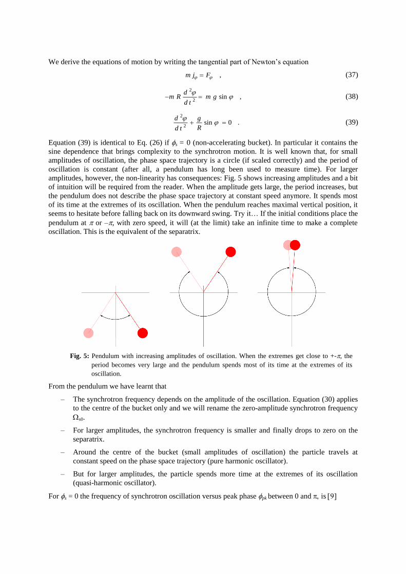
Equation (39) is identical to Eq. (26) if s = 0 (non-accelerating bucket). In particular it contains the

sine dependence that brings complexity to the synchrotron motion. It is well known that, for small

amplitudes of oscillation, the phase space trajectory is a circle (if scaled correctly) and the period of

oscillation is constant (after all, a pendulum has long been used to measure time). For larger

amplitudes, however, the non-linearity has consequences: Fig. 5 shows increasing amplitudes and a bit

of intuition will be required from the reader. When the amplitude gets large, the period increases, but

the pendulum does not describe the phase space trajectory at constant speed anymore. It spends most

of its time at the extremes of its oscillation. When the pendulum reaches maximal vertical position, it

seems to hesitate before falling back on its downward swing. Try it… If the initial conditions place the

pendulum at or –, with zero speed, it will (at the limit) take an infinite time to make a complete

oscillation. This is the equivalent of the separatrix.

Fig. 5: Pendulum with increasing amplitudes of oscillation. When the extremes get close to +-, the

period becomes very large and the pendulum spends most of its time at the extremes of its

oscillation.

From the pendulum we have learnt that

– The synchrotron frequency depends on the amplitude of the oscillation. Equation (30) applies

to the centre of the bucket only and we will rename the zero-amplitude synchrotron frequency

s0.

– For larger amplitudes, the synchrotron frequency is smaller and finally drops to zero on the

separatrix.

– Around the centre of the bucket (small amplitudes of oscillation) the particle travels at

constant speed on the phase space trajectory (pure harmonic oscillator).

– But for larger amplitudes, the particle spends more time at the extremes of its oscillation

(quasi-harmonic oscillator).

For s = 0 the frequency of synchrotron oscillation versus peak phase pk between 0 and is

0

2

120

2 2

.

2

1 sin sin2

ss pk

pk

du

u

(40)

It is plotted in Fig. 6, together with an approximation (very) valid for moderate amplitudes

2

0 1 .4

pks pk s

(41)

Fig. 6: s/s0 as a function of the maximum phase deviation in radian. Exact

formula (bottom trace, blue) and approximation Eq. (41). Non-

accelerating bucket (s = 0).

Analysis

– Given its length, the bunch will have a spread in the synchrotron tunes of the various particles.

The longer the bunch, the larger the tune spread (for a given RF frequency).

– In hadron machines this tune spread will provide a stabilizing mechanism against coherent

instabilities, called Landau damping.

– Harmonic RF systems: Adding an harmonic system (2 × or 4 × RF) we can shape the

synchrotron tune vs. peak deviation curve. We may wish to increase the spread to increase

Landau damping for stability (200/800 MHz systems in the SPS for example). Or we may

wish to reduce the spread, to make the potential more linear and reduce the filamentation at

injection (see below). Both are possible by adjusting the relative amplitude and phase of the

fundamental and harmonic.

During filling, if the bunch is injected off-centred in the receiving bucket, its shape will be modified as

the particles have different synchrotron frequencies: the trajectories in phase space will be travelled at

different speed, fast for the particles around the centre of the bucket and slow for the ones injected

close to the separatrix. Parts of the bunch will lag behind the core, resulting in filamentation in phase

space (Fig. 7). After complete filamentation, the emittance will be much larger, filling the entire space

within the blue trace in the simulation shown on Fig. 7.

Fig. 7: Simulation of the filamentation at injection in the LHC bucket

(phase space in [momentum, phase] units, above transition and thus

clockwise displacement on the trajectories). The bunch is injected

with a small phase/momentum error. The separatrix is in red. The

evolution is left to right and top to bottom. After filamentation the

bunch will fill the full area inside the blue contour resulting in an

almost-full bucket. Courtesy of J. Tuckmantel.

1.5 RF capture optimization

We consider bunch-into-bucket transfer: the bunches must be transferred from the buckets of an

injecting machine into the middle of the buckets in the receiving machine. In accelerator chains the

optimal RF frequency tends to increase with energy so that the width of the receiving bucket is much

smaller than the width of the injecting bucket if expressed in seconds. So the tolerance to phase errors

is small. In the SPS–LHC case we transfer from a 200.4 MHz bucket into a 400.8 MHz bucket. We

assume that the two RF systems are properly locked together. See Refs. [10] and [11] for technical

details on RF synchronization between synchrotrons.

As the momentum and charge do not change in the transfer line, Eq. (5) requires

1 1 2 2 ,B B (42)

where index 1 and 2 refer to the two machines. Coarse matching of the two magnetic fields is first

done with RF OFF: the beam is injected and the trajectories are measured on the first few turns in the

receiving machine. Then using Eq. (16) one can derive the trim on B2 that will centre the average

beam trajectory.

Once the magnetic fields are matched we can switch the RF ON and move to the fine

adjustments of the RF parameters of the receiving machine: frequency, phase, and voltage. The

capture simulated on Fig. 7 is a catastrophe: the injected bunch density is colour-coded with dark red

for the dense core and light yellow for the edges. It is injected with a phase and momentum error.

Recall that momentum and frequency are equivalent at constant B field, Eq. (18). As explained in the

figure caption, it will filament and finally fill most of the bucket. As a result the bunch emittance has

been blown up by a factor four to five during transfer and we end up with a significant population very

close to the separatrix, ready to be lost out of the bucket at the weakest perturbation. So we need to

inject in the centre of the bucket and that calls for fine-adjustment of the RF frequency and phase.

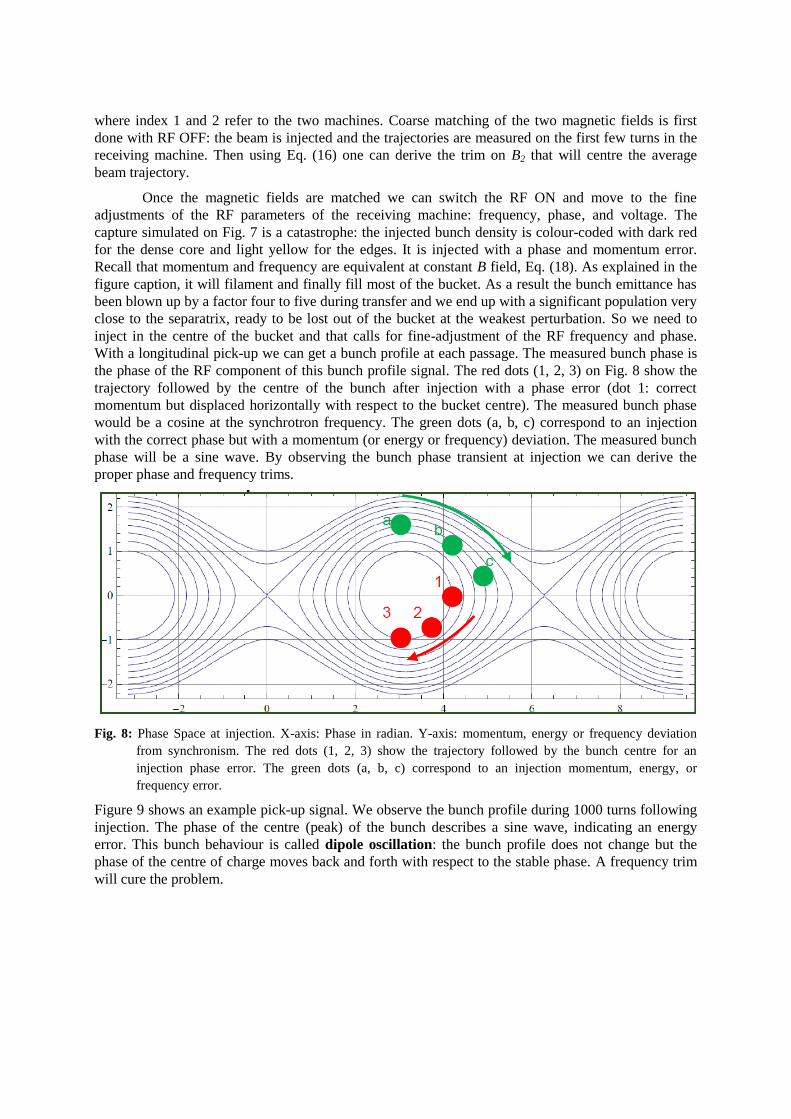
With a longitudinal pick-up we can get a bunch profile at each passage. The measured bunch phase is

the phase of the RF component of this bunch profile signal. The red dots (1, 2, 3) on Fig. 8 show the

trajectory followed by the centre of the bunch after injection with a phase error (dot 1: correct

momentum but displaced horizontally with respect to the bucket centre). The measured bunch phase

would be a cosine at the synchrotron frequency. The green dots (a, b, c) correspond to an injection

with the correct phase but with a momentum (or energy or frequency) deviation. The measured bunch

phase will be a sine wave. By observing the bunch phase transient at injection we can derive the

proper phase and frequency trims.

Fig. 8: Phase Space at injection. X-axis: Phase in radian. Y-axis: momentum, energy or frequency deviation

from synchronism. The red dots (1, 2, 3) show the trajectory followed by the bunch centre for an

injection phase error. The green dots (a, b, c) correspond to an injection momentum, energy, or

frequency error.

Figure 9 shows an example pick-up signal. We observe the bunch profile during 1000 turns following

injection. The phase of the centre (peak) of the bunch describes a sine wave, indicating an energy

error. This bunch behaviour is called dipole oscillation: the bunch profile does not change but the

phase of the centre of charge moves back and forth with respect to the stable phase. A frequency trim

will cure the problem.

Fig. 9: Mountain range display: bunch profile measured turn after turn following

injection. Horizontal axis in ns. Vertical axis in turn number (1000 turns total).

The first few traces are recorded just before injection.

Be aware that, as the injector RF is locked to the receiving machine for transfer, a trim of the

receiving RF frequency will also change the situation in the injector (small radial displacement at top

energy and small change in the momentum at transfer). This may call for re-adjustment of the

magnetic field in both machines. In theory, from a proper application of Eqs. (12) to (15) to the two

machines, one could implement perfect energy matching in a single trial but I have observed that

several iterations were always needed for a good result. The magnetic field and RF frequency are well

adjusted when both first turn and beam circulating after injection transient, are centred.

Let us now consider matching the RF voltage at injection. Figure 10 shows the capture of a

bunch (marked in red) with perfect phase and energy matching. The centre of the bunch falls in the

middle of the bucket. The bunch has a non-zero length and therefore occupies an area defined by the

phase space trajectories in the injector. But it is not matched to the phase space trajectories in the

receiving machine (the voltage is too high). The particles of the bunch will follow these trajectories,

resulting in the evolution shown on the figure: after one-quarter synchrotron period, the bunch length

has been reduced (projection on the phase axis) and the momentum spread has been increased. We call

this a quadrupole oscillation. It is a modulation of the bunch length (and momentum spread) at twice

the synchrotron frequency. After filamentation the bunch emittance will be much increased and this

must be avoided.

Fig. 10: Evolution in phase space. injection of a bunch (dark red) in the exact centre

of the bucket but with phase space trajectories mismatched to the two-

dimensional phase-momentum bunch profile. The result is a quadrupole

oscillation at twice the synchrotron frequency and, after filamentation,

significant emittance increase.

Figure 11 shows the time evolution of the bunch profile at injection with voltage mismatch. It

corresponds to the phase space shown on Fig. 10. The voltage here is too high, resulting in a reduction

of bunch length first. If the voltage was too low, the bunch length would first increase.

Fig. 11: Mountain range display: quadrupole oscillation at injection (plus some

dipole and loss) indicating a voltage mismatch. Voltage too high.

Voltage matching is very easy. Feeding the longitudinal pick-up signal into a simple peak-

detector, we get a monitoring of the bunch profile peak over time. In the absence of loss the product of

bunch peak and length is constant. So quadrupole oscillations are clearly visible at the peak-detector

output. Figure 12 shows this signal at the LHC injection for two different RF voltages, mismatched on

the left and matched on the right.

Fig. 12: Peak-detected pick-up signal showing quadrupole oscillation. Left: 8 MV. Right: 2.5 MV.

The RF voltage should be matched at capture to preserve the longitudinal emittance. In high-

intensity machines, however, a larger voltage helps fight the effect of beam loading. If the emittance

budget allows for some blow-up during transfer, we would then best capture with an higher-than-

matched voltage. In 2010 we operated the SPS–LHC transfer with 3.5 MV while Fig. 12 shows that

2.5 MV would be matched best.

1.6 Radiation damping

When a relativistic charged particle is accelerated (meaning that its speed vector changes) it radiates

energy at a rate proportional to the square of the accelerating force. In a circular accelerator the main

accelerating force is the bending of the trajectory. For a particle moving at constant speed on a circular

orbit of radius the power radiated is

4 4

0 0 2

2,

3P r E c

(43)

where r0 is the particle classical radius. The radiated energy must be compensated by the RF voltage.

At 104.5 GeV/c per beam, LEP required 3.66 GV RF. In the presence of significant radiation loss, the

stable phase will not be zero (or 180 degrees) even if the magnetic field is constant. The energy lost by

the synchronous particle must be compensated by a corresponding acceleration in the cavities. Notice

that the radiated power increases sharply with energy (fourth power). During a synchrotron period in

phase space, the mechanism will have a damping effect on the synchrotron oscillation of the non-

synchronous particle: when its energy is larger than the synchronous energy it will radiate more and

thereby lose part of the excess. Then in the bottom half of its synchrotron oscillation where its energy

is lower than the synchronous energy, it will radiate less, thereby reducing its energy deviation

(Fig. 13). This is modeled as a damping rate in the synchrotron motion equation

220

22 sin sin 0 .

cos

ss

s

d d

d td t

(44)

The damping term is proportional to the derivative of P with respect to and, after some

manipulations, we get a simple and elegant approximated expression for the damping rate [2], [4], [5]

,s

s

P

E

(45)

where Ps is the power radiated by the synchronous particle. The damping time is thus the time that it

would take for the synchronous particle to radiate out all its energy. Radiation damping is significant

for circular electron accelerators and storage rings only because the radiated power scales as 4 and

hadrons are not relativistic enough yet. In the LHC the radiation damping time is ~24 hours at 7 TeV/c

and ~ 384 hours (more than two weeks) at the reduced 3.5 TeV/c used in 2010. Not much damping!

The 7 TeV/c protons in the LHC have ~ 7000 while the 100 GeV/c electrons and positrons in LEP

had ~ 200 000.

Fig. 13: Phase space trajectory of a non-synchronous particle with

radiation damping. Evolution predicted from Eq. (44).

Where significant, radiation damping has a decisive impact on the bunch profile. With the

damping introduced above, all non-synchronous particles would slowly spiral in phase space as shown

on Fig. 13, converging to the centre of the bucket, resulting in zero longitudinal emittance and a point-

like bunch. This is not the case. Radiation damping does indeed lead to very short, but not point-like,

bunches in high-energy lepton storage rings. Electromagnetic radiation is emitted in quanta of discrete

energy. In the phase-space representation, when a quantum is emitted, the momentum of the particle

changes and it jumps on another, lower energy trajectory. This brings the bunch closer to the centre of

the bucket if the quantum was emitted in the excess-energy part of the trajectory, but away from

synchronism if emitted in the lower-energy part. This is similar to the classic statistical random walk

process: at each trial we can take one step forward or backward. After a large number of trials, the

average position is still zero but the variance keeps growing. The effect of many small jumps in phase

space creates diffusion. The bunch length will be an equilibrium between the damping and the

excitation due to the stochastic nature of the process. Refer to Refs. [4] and [5] for a detailed

presentation. The bunch profile is also shaped by the radiation emission: for a given particle,

emissions of successive quanta are independent. The central limit theorem states that, if a random

variable is the sum of a large number of independent variables, its distribution becomes Gaussian no

matter what the distribution of the individual random variables is. In high-energy lepton storage rings

the bunch profile is indeed Gaussian and the distribution can be characterized by a single number

(usually the variance of the longitudinal bunch profile in either length or time, as measured by a

longitudinal pick-up). That is not the case in hadron machines where the bunch profile depends greatly

on the manipulations suffered in the acceleration chain.

1.7 Adiabatic evolution

So far we have considered the synchronous particle parameters (ps, Es, s) and the RF voltage as

constant and have moved them out of the time derivatives. In an accelerator these parameters vary

during the ramp. The voltage is matched to the injector at capture, then increased during the ramp to

keep a sufficient bucket area with a non-zero (or 180 degrees) stable phase. The evolution is adiabatic

if the relative variation of the synchrotron frequency in one synchrotron period is small

0

1

0 0

2.

s

s s

d

dt e

(46)

In that case the particle stays on the same trajectory in phase space as this trajectory slowly adapts to

the changing bucket. The Boltzman–Ehrenfest adiabatic theorem can be applied [2]: ―If (p,q) are

canonically conjugate variables of an oscillatory system with slowly changing parameters, then the

action integral, evaluated over one period of oscillation, is constant.‖

I = pdqò =C . (47)

Applying this theorem to a closed trajectory in the longitudinal phase space we get the following

relations describing the evolution of the maximum time tpk and energy Epk deviations in E–t phase

space, valid for adiabatic ramping (changes of Es) and adiabatic voltage (V) variations:

41

,cos

pkRF s

tf V

(48)

4cos

.spk RF

VE f

(49)

Apart from the singularity at transition (= 0), bunch length shrinks and energy spread increases with

voltage increase and slow ramping (constant stable phase), if adiabatic. The effect is, however,

moderate (fourth root). For the handling of the singularity at transition, see Ref. [2]. Figure 14 shows

the evolution of the LHC bunch length (4 ) during adiabatic manipulations: voltage increase before

the start of the magnetic ramp (resulting in a sharp bunch shortening), followed by ramping.

Fig. 14: Bunch length evolution for both beams in one early LHC ramp: capture at 450 GeV/c with 3.5 MV,

voltage increase to 5 MV before start ramp then rise to 8 MV in the first part of the ramp (up to

3.5 TeV/c). Bunch length (4) evolution. Beam 1: 1.82 ns -> 1.61 ns -> 0.83 ns / Beam 2: 1.75 ns

-> 1.58 ns -> 0.77 ns

Applying Eqs. (48) and (49) to the outer trajectory of the bunch in E–t phase space we conclude that

the longitudinal emittance (in eVs) remains constant during adiabatic evolution.

2 Beam-based loops for synchrotrons

In this section, we study control loops that use signals from beam pick-ups, either longitudinal (beam

phase) or transverse (beam position) and that act on all bunches.

2.1 Beam-phase loop

In the previous section we saw that phase/energy/voltage mismatch at capture will trigger dipole or

quadrupole oscillations resulting in emittance blow-up after filamentation. In static conditions, the RF

noise will excite the synchrotron oscillation of each particle individually, with the same result. In

electron machines the synchrotron radiation provides a natural damping mechanism and will be

sufficient in most cases except for the injection transient. In proton and ion machines there is no such

natural damping. The bunch lengthening caused by the RF noise may lead to beam loss when particles

reach the separatrix (major concern in colliders where beams are kept colliding for several hours). The

beam-phase loop is designed to damp the dipole oscillation of the bunch.

Let us first consider the synchrotron oscillation in presence of a small RF modulation of the

RF frequency. The kinematic relation for the RF phase at cavity crossing time, Eq. (20), becomes

2 .rev RF

dh f

dt

(50)

The first term is the effect of the momentum error and the second term is the RF frequency

modulation. Following the derivation of the previous section, we get a modified linearized synchrotron

motion equation

2

202

.RFs

d d

dtd t

(51)

The phase of the beam is defined as the phase of the Fourier component of the beam current at the RF

frequency. If the buckets are not evenly filled around the machine, the beam current will have a

strong amplitude modulation at the revolution frequency. Its spectrum thus shows side-bands at

frf ± nfrev. These must be filtered out of the beam phase signal to avoid exciting higher order coupled

bunch dipole oscillations, (n > 0) with the phase loop.

Fig. 15: Beam-phase loop

Consider the LLRF system shown on Fig. 15: a longitudinal pick-up provides a measurement of the

beam phase that is compared to the phase of the cavity field (or to the vectorial sum of the cavity

fields, with proper compensation for the time of flight, if the accelerator contains several cavities). The

difference (beam–cavity phase error) minus the stable phase is used to correct the RF frequency via

the phase loop amplifier. The inherent delays and bandwidth limitations in the beam-phase loop make

it impossible to act bunch per bunch. We assume that the beam phase is, at each turn, averaged over

all bunches in the machine. The simplest regulation is proportional only. s is the RF frequency (in

rad/s) derived from a measurement or an estimation of the magnetic field, Eq. (8). rf is the

correction applied by the phase loop. We have

~kRF (52)

where the brackets stand for averaging over all bunches. The equation of synchrotron motion becomes

2

202

0 .s

d dk

d td t

(53)

The synchrotron frequency is not changed but we have introduced the desired damping term. The

above equation much resembles the damped equation resulting from radiation, Eq. (44). However,

while radiation damps each particle individually, the LLRF phase loop can only act on the average

dipole oscillation of all bunches. It must be fast compared to the filamentation time in order to damp

phase and energy errors at injection before significant emittance blow-up. Figure 16 illustrates the

action of the phase loop in normalized phase space. It considers injection in a non-accelerating bucket

above transition. The point-like test bunch is injected at point (0, 1) in the normalized phase space,

corresponding to a - phase error and a momentum error equal to one half the bucket half-height.

(The bucket is shown at the top left.) Displayed are the evolutions without phase loop (top right)

resulting in no capture, and with phase loop for two different loop gain settings. These plots are

somewhat confusing however: recall that the phase loop does not displace the beam. It changes the

RF phase and frequency to jump the bucket onto the injected bunch. In Fig. 16 the phase loop actually

displaces the axis to bring the (, 0) point right on the beam. This explains why a phase loop can

be much faster than the synchrotron period while remaining adiabatic.

Fig. 16: Injection transients in normalized phase space (, 1/ s d/dt) above transition for synchronous

phase 180 degrees. RF bucket (top left). Injection of a point-like bunch with phase and energy

error point (0, 1). The evolution without phase loop is shown on the top right: the bunch surfs over

the bucket and is not captured. The bottom two traces are with phase loop on at low gain (left) and

high gain (right): the bunch is captured.

Figure 17 shows the fast damping of the LHC injection error, achieved with the phase loop.

Fig. 17: Damping of the phase error at injection into the LHC. Single bunch (89 s revolution period). Left:

beam–cavity phase error, 500 s/Div. After a four-turn latency, the error is brought to zero in

about ten turns. Right: mountain range of the bunch at injection showing the fast damping of the

phase error. The bunch profile is colour-coded. Notice the quadrupole oscillation caused by a

voltage mismatch.

After injection, in quiet conditions, the phase loop is very efficient in fighting the effect of RF

noise. This is important in hadron colliders where beams must be kept for several hours with minimal

emittance blow-up and there is no natural damping. RF phase noise is more damaging than amplitude

noise as the synchrotron phase is practically zero or 180 degrees in hadron colliders. The effect of RF

noise can be observed by monitoring the bunch length. Figure 18 shows the clear correlation between

bunch lengthening and phase loop gain in the LHC. A strong phase loop was also essential in the SPS

when used as p–pbar collider. Be aware that the phase loop is useful only if the bunch fills a small

portion of the bucket. With a full bucket any injection error or RF noise will result in particles

escaping.

Fig. 18: LHC single bunch at 3.5 TeV/c, 1E10 p. Evolution of bunch length with time while varying the

phase loop gain [12].

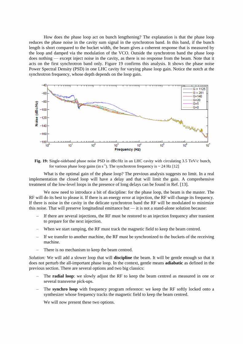
How does the phase loop act on bunch lengthening? The explanation is that the phase loop

reduces the phase noise in the cavity sum signal in the synchrotron band. In this band, if the bunch

length is short compared to the bucket width, the beam gives a coherent response that is measured by

the loop and damped via the modulation of the VCO. Outside the synchrotron band the phase loop

does nothing — except inject noise in the cavity, as there is no response from the beam. Note that it

acts on the first synchrotron band only. Figure 19 confirms this analysis. It shows the phase noise

Power Spectral Density (PSD) in one LHC cavity for varying phase loop gain. Notice the notch at the

synchrotron frequency, whose depth depends on the loop gain.

Fig. 19: Single-sideband phase noise PSD in dBc/Hz in an LHC cavity with circulating 3.5 TeV/c bunch,

for various phase loop gains (in s-1

). The synchrotron frequency is ~ 24 Hz [12]

What is the optimal gain of the phase loop? The previous analysis suggests no limit. In a real

implementation the closed loop will have a delay and that will limit the gain. A comprehensive

treatment of the low-level loops in the presence of long delays can be found in Ref. [13].

We now need to introduce a bit of discipline: for the phase loop, the beam is the master. The

RF will do its best to please it. If there is an energy error at injection, the RF will change its frequency.

If there is noise in the cavity in the delicate synchrotron band the RF will be modulated to minimize

this noise. That will preserve longitudinal emittance but — it is not a stand-alone solution because:

– If there are several injections, the RF must be restored to an injection frequency after transient

to prepare for the next injection.

– When we start ramping, the RF must track the magnetic field to keep the beam centred.

– If we transfer to another machine, the RF must be synchronized to the buckets of the receiving

machine.

– There is no mechanism to keep the beam centred.

Solution: We will add a slower loop that will discipline the beam. It will be gentle enough so that it

does not perturb the all-important phase loop. In the context, gentle means adiabatic as defined in the

previous section. There are several options and two big classics:

– The radial loop: we slowly adjust the RF to keep the beam centred as measured in one or

several transverse pick-ups.

– The synchro loop with frequency program reference: we keep the RF softly locked onto a

synthesizer whose frequency tracks the magnetic field to keep the beam centred.

We will now present these two options.

2.2 Radial loop

Figure 20 shows the combination of phase and radial loop. One (or several) transverse pick-ups

provide a measurement of the beam radial position error that is used to correct the frequency via the

radial loop amplifier.

Fig. 20: A classic combination for proton and ion synchrotrons: phase loop and radial loop

The simplest regulation is proportional only. We have

.RF Rk k R (54)

At constant magnetic field, the radial displacement is proportional to the momentum deviation. From

Eq. (12)

p

p

R

R

t

~1

~

2

(55)

and the frequency trim becomes

2

.RF R

t s

Rk k p

p

(56)

Using Eqs. (51) and (23), we get, after linearization

2

202 2

cos0 .

2

sRs

s t

d d qVk k

d td t p

(57)

Analysis:

– The radial loop does not provide damping. It only increases the frequency of oscillation. The

damping is provided by the phase loop.

– The phase loop/radial loop tandem has very good behaviour during transients. At injection, for

example, if the beam is injected with a phase and energy error the first turn will be on an off-

centred orbit and the beam will see a non-zero RF voltage. The phase loop reacts in a few

turns and the RF jumps on the bunch, thereby preventing emittance blow-up. Thereafter the

radial loop will slowly modify the beam energy to drive it back to the centre orbit.

– In the system shown on Fig. 20, the stable phase s must be subtracted from the beam–cavity

phase error measured by the phase discriminator. It is computed from a measurement of the

RF voltage and the momentum, Eq. (11). An error in the stable phase computation will

introduce a radial displacement of the beam if the phase-loop amplifier is DC-coupled. To

avoid this, the phase loop can be AC-coupled. This method is used in the PS accelerator at

CERN [14].

– If one neglects the delays, the combination of phase loop/radial loop is unconditionally stable.

A comprehensive treatment of the low-level loops in the presence of delays can be found in

Ref. [13]. Other interesting references are [15], [16] (application to the CERN PS during the

1970s), and [17] (application to the CERN PS Booster).

– The sign of the radial gain must be changed at transition because cos s changes sign. It must

be positive below transition and negative above.

– The radial loop is very efficient for reducing the effect of frequency errors on the radial

position. Let us assume a small error in the RF frequency. From Eq. (17) we derive the

resulting error on the radial position (without radial loop)

2

2 2.

t

R

R

(58)

At transition, the sensitivity becomes infinite! With the radial loop the effect is limited by the

closed loop gain, that cannot be too large in order to remain adiabatic. The radial loop is

required to cross transition.

– The radial loop couples the transverse and longitudinal planes using transverse measurements

to estimate momentum and correct the frequency. This causes problems: transverse betatron

oscillations are interpreted as momentum error. This effect can be minimized by using two

pick-ups at 180 degrees in betatron phase.

– The radial loop typically looks at one or few PUs only. It centres the beam in one location

only, instead of centring the average orbit.

2.3 Synchro loop

Instead of monitoring the beam radial position we can lock the RF frequency on an external reference

via a synchro loop. This loop must have a much smaller gain than the phase loop to guarantee

adiabaticity. Figure 21 shows the combination of phase and synchro loop. We measure the phase of

the RF (or beam) and compare it with the reference generator. This error is used to correct the RF

frequency via the synchro loop amplifier. The reference generator will be set at the injection frequency

during filling, then follow the frequency program during ramping, Eq. (8), and finally be locked to the

receiving machine if needed for transfer.

Fig. 21: Another classic combination for proton and ion synchrotrons: phase loop and synchro loop

The overall system is described by a third-order differential equation. Its analysis is easier if we use

Laplace transforms. First the beam transfer function (undamped resonator at s0), from Eq. (51)

22

0

( ) ( ) ( ) .RF

s

ss s B s

s

(59)

The open-loop transfer function from RF to RF (the phase modulation applied to the RF) with

phase loop closed but synchro loop open is

2 20

2 20

( ) 1 1( ) .

( ) 1 ( )

RF s

olRF s

s sH s

s k B s s s s k s

(60)

If the synchro loop amplifier is proportional only, the response gives too low a phase margin. It can be

corrected by using a phase advance network as corrector in the synchro loop amplifier

1

( ) .1

sync sync

a sH s k

s

(61)

Figure 22 shows the Nyquist plot without and with the corrector. The parameters a and can be

optimized using classical controls theory to provide the usual 60 degrees phase margin. They will

depend on the synchrotron frequency and, if this one varies much during the acceleration, the corrector

parameters must track.

Fig. 22: Nyquist plots of Hol(j).Hsync(j) without phase advance network (left) and with correction

optimized. Phase margin increased from ~45 to >60 degrees.

Analysis:

– The synchro loop must respond in a time that is larger than the synchrotron period to remain

adiabatic and to avoid exciting the beam with noise around the synchrotron frequency.

– The loop can be used throughout the acceleration cycle: it is set at the injection frequency

during filling, then ramped following either a measurement of the magnetic field (SPS proton

for LHC) or a function if the magnetic field is well modelled (LHC).

– If the accelerator is an injector, the loop can remain in use while rephasing takes place locking

the reference generator on the receiving machine RF (SPS proton for LHC).

– If it is a collider, using a single reference for both rings from filling to physics, makes the

beam cross in the correct position from injection on (LHC).

– If needed, a slow measurement of the orbit displacement using all ring transverse horizontal

PUs can feed back on the reference frequency (LHC real-time orbit correction).

– Limitation: It is not practical if transition is crossed during the acceleration. Equation (58)

shows that, near transition, a very small frequency error will cause a large radial displacement.

The radial loop is preferred if the acceleration cycle crosses transition.

– Limitation: The range of the phase discriminator is 360 degrees only. And the synchro loop

is much slower than the phase loop to remain adiabatic. At injection, with large offsets

(energy error or stable phase offset), the phase discriminator may reach its limits before the

loop is locked. It will later lock with an error of one or several RF periods. This is not

acceptable if the filling requires successive injections. In the LHC the drifts are very small and

the offsets do not result in a synchro transient exceeding ± 180 degrees. The situation is

different in the SPS where analog electronics is still in use and offsets vary much more from

injection to injection. The problem has been solved by implementing the synchro loop at a

sub-harmonic of the RF (40 MHz = fifth sub-harmonic). The 360 degrees range at the sub-

harmonic virtually implements a multi-period phase range at the RF frequency.

The phase loop/synchro loop tandem performs very well in the LHC. We inject at 450 GeV/c, well

above transition (~ 50 GeV/c). Figure 23 shows the injection transients: phase loop error on the left

and synchro loop error on the right. The time is scaled in turns. Notice the different scales. The fast

phase loop ‗jumps‘ the RF on the beam in about ten turns, nulling any phase and energy error. In the

presence of an energy error, the RF frequency will thus be driven away from the reference frequency

as it follows the off-energy beam. The result is the observed linear phase ramp in the synchro loop

error. After about three hundred turns (27 ms), the synchro loop has reacted slowly and brought the RF

and beam back to the reference. Figure 23 is a screenshot of the display used by the LHC operation to

monitor LLRF injection transients.

Fig. 23: LHC phase loop (left) and synchro loop (right) injection transients. Beam 1 (top) and beam 2 (bottom).

Horizontal axis in turns (89 s revolution period). Notice the different scales. Synchrotron frequency

around 60 Hz.

Instead of using the RF phase one could implement a synchro loop comparing the beam phase

with the reference generator. This adds a complication if the beam intensity covers a wide dynamic

range: the design of a zero phase-shift limiter. The dynamics are similar but different. Refer to Refs.

[14] and [17] for details.

References

[1] John J. Livingood, Principles of Cyclic Particle Accelerators (Van Nostrand, New York, 1961).

[2] H. Brück, Accélérateurs circulaires de particules (Presses Universitaires de France, Paris, 1966).

[3] C. Bovet et al., A Selection of Formulae and Data Useful for the Design of A.G. Synchrotrons,

rev. version, CERN-MPS-SI-INT-DL-70–4 (CERN, April 23, 1970).

[4] S. Y. Lee, Accelerator Physics, 2nd

ed. (World Scientific, Singapore, 2004).

[5] H. Wiedemann, Particle Accelerator Physics, 3rd

ed. (Springer, Berlin, 2007).

[6] J. Le Duff, Longitudinal beam dynamics, CERN Accelerator School: Basic Course on General

Accelerator Physics, Loutraki, Greece, 2000, CERN 2005–004.

[7] W. Pirkl, Longitudinal beam dynamics, CERN Accelerator School: Fifth Advanced Accelerator

Physics Course, Rhodes, Greece, 1993, CERN 95–06.

[8] L. Rinolfi, Longitudinal beam dynamics, Application to Synchrotron, CERN/PS 2000–008

(LP), Joint Universities Accelerator School (JUAS), April 2000.

[9] A. W. Chao and M. Tigner, Handbook of Accelerator Physics and Engineering (World

Scientific, Singapore, 1999).

[10] R. Garoby, Timing aspect of bunch transfer between circular machines. State of the art in the PS

complex, PS/RF/Note 84–6, December 1984.

[11] P. Baudrenghien et al., SPS beams for LHC: RF beam control to minimize rephasing in the

SPS, EPAC 98, Stockholm, Sweden.

[12] T. Mastorides et al., LHC beam diffusion dependence on RF noise: models and measurements,

IPAC 2010, 23–28 May 2010, Kyoto, Japan.

[13] S. Koscielniak, RF systems aspects of longitudinal beam control (in the low current regime), US

Particle Accelerator School, 1989–90, M. Month and M. Dienes eds., AIP conference

proceedings 249 (AIP, New York, 1992) Vol. 1, p. 89.

[14] R. Garoby, Low level RF and feedback, Proc. Joint US-CERN-Japan International School,

Frontiers of Accelerator Technology, Tsukuba, 1996.

[15] D. Boussard, Une présentation élémentaire du système Beam Control du PS [An elementary

presentation of the PS Beam Control System], MPS/SR/Note/73–10 (1973).

[16] W. Schnell, Equivalent circuit analysis of phase-lock beam control systems, CERN 68–27

(1968).

[17] P. Baudrenghien, Low-level RF systems for synchrotrons, Part I, CERN Accelerator School:

Radio Frequency Engineering, Seeheim, 2000, CERN 2005–003.

Appendix A: Relations between E (total energy), E0 (rest energy), p (momentum), v

(speed), and

0

2

2

22 2 20

2

2

0

0

0

11

1

1

1

1

938.26 MeV proton rest energy

0.511 MeV electron rest energy

p

e

v

c

E

E

E E c p

dE p cv

dp E

E

cp

E

E