instructor: zhou, xin february 15, 2018web.math.ucsb.edu/~zhou/math241a_2017.pdfp 2, and smooth map...

Notes on Minimal Surface

Instructor: Zhou, Xin

February 15, 2018

Contents

1 Preliminary 3

2 Minimal Graph 4

3 The Calibration Properties 73.1 Calibrated property of minimal graphs . . . . . . . . . . . . . 73.2 A general calibrated argument . . . . . . . . . . . . . . . . . 8

4 First Variation 104.1 First Variation Formula . . . . . . . . . . . . . . . . . . . . . 104.2 Examples . . . . . . . . . . . . . . . . . . . . . . . . . . . . . 114.3 Convex hull property . . . . . . . . . . . . . . . . . . . . . . . 124.4 Fluxes . . . . . . . . . . . . . . . . . . . . . . . . . . . . . . . 12

5 Monotonicity formula and Bernstein Theorem 145.1 Monotonicity formula . . . . . . . . . . . . . . . . . . . . . . 145.2 Bernstein’s theorem (n=2) . . . . . . . . . . . . . . . . . . . . 16

6 Second variation and Stability 196.1 Second Variation of Volume . . . . . . . . . . . . . . . . . . . 196.2 Jacobi operator and Stability . . . . . . . . . . . . . . . . . . 21

7 Additional Topics in Stability I 25

8 Criterion for stability 28

9 The Generalized Bernstein Theorem 329.1 Bochner Technique . . . . . . . . . . . . . . . . . . . . . . . . 329.2 Proof of Generalized Bernstein Theorem . . . . . . . . . . . . 35

10 Curvature Estimate 37

1

CONTENTS 2

11 Choi-Schoen’s Theorem 40

12 Small Curvature implies Graphical 44

13 Schoen’s Curvature Estimate 47

14 Bernstein’s Theorem and Minimal Cone 51

15 The Topology of Minimal surface 56

16 Closed Minimal Surfaces in S3 60

17 General Relativity 6317.1 Einstein Equations . . . . . . . . . . . . . . . . . . . . . . . . 6417.2 Initial value problem . . . . . . . . . . . . . . . . . . . . . . . 64

17.2.1 Derivation of (CE) . . . . . . . . . . . . . . . . . . . . 6517.3 Asymptotical Flatness . . . . . . . . . . . . . . . . . . . . . . 65

18 Geometric Measure Theory and Minimal Surfaces 67

Chapter 1

Preliminary

Absent for the first 20 minutes.Let Σ ⊂ (Mn, g) be a hypersurface of an n-dimensional Riemannian man-ifold (Mn, g), where D is the corresponding Riemannian connection. Letg|Σ be the induced metric. Given tangent vectors X,Y of Σ, the secondfundamental form II, which is a vector valued symmetric 2-tensor on Σ, isdefined as:

II(X,Y ) = (DXY )⊥.

Definition 1.1 (Mean Curvature). The mean curvature of Σ is defined asthe trace of the second fundamental form II, which is

H = trII(X,Y ) = II(ei, ei),

where ei are orthonormal basis of TΣ.

Proposition 1.2. Assume M is a n-dimensional manifold, and Σ is a .Let X be the normal on Σ, i.e. X(p) ⊥ TpΣ for any p ∈ Σ, then we havedivΣX = − < X,H > .

Proof.

divΣX =< DeiX, ei >= − < X,Deiei >

= − < X, (Deiei)⊥ >= − < X,H >

3

Chapter 2

Minimal Graph

Let Ωn−1 ⊂ Rn−1 is a domain, u : Ω 7→ R1 is a smooth function with |∇u| 6=0, then, the graph of u, denoted Σu = (x, u(x)) : x = (x1, ..., xn−1) ∈ Ω.Let F : Ω 7→ Rn, F (x) = (x, u(x)) be the C∞ embedding of Σu = F (Ω)to Rn. Then, we are going to compute the volume form of Σu with localchart (F (Ω), F−1). Let g be the induced metric of Euclidean Space Rn onΣ. Hence, we have

g(∂

∂xi,∂

∂xj) =<

∂F

∂xi,∂F

∂xj>= δij +

∂u

∂xi

∂u

∂xj,

i.e.g = I +∇u(∇u)T .

Moreover, since

g∇u = (I +∇u(∇u)T )∇u = ∇u+∇u∇uT∇u= ∇u+∇u(∇uT∇u) = ∇u+ |∇u|2∇u= (1 + |∇u|2)∇u

(2.1)

we know that 1 + |∇u|2 is a eigenvalue of g with eigenvector ∇u. SinceRank(g − I) = Rank(∇u(∇u)T ) = 1, we know that 1 is also a eigenval-ue of g with multiplicity of n − 2. Since g is symmetry, we could finde2, ..., en−1,Hence det(g) = 1 + |∇u|2. Let dx = dx1...dxn−1, we now havevolume form dvol =

√det(g)dx =

√1 + |∇u|2dx.

By now, we can see that

Area(Σu) =

∫Ω

√1 + |∇u|2dx.

4

CHAPTER 2. MINIMAL GRAPH 5

Let η ∈ C∞c (Ω), we then consider Area(Σu+tη), if the graph Σu is minimal,we must have d

dtArea(Σu+tη)|t=0 = 0 for any η ∈ C∞c (Ω). Hence, we compute

d

dtArea(Σu+tη)|t=0 =

d

dt

∫Ω

√1 + |∇(u+ tη)|2dx|t=0 =

∫Ω

d

dt

√1 + |∇(u+ tη)|2dx|t=0

=

∫Ω

(∇u+ t∇η)∇η√1 + |∇(u+ tη)|2

dx|t=0 =

∫Ω

∇u∇η√1 + |∇u|2

dx

= −∫

Ωηdiv(

∇u√1 + |∇u|2

),

where the last equality follows from Stoke Formula. Hence, we can see thatif Σu is minimal graph, we must have div( ∇u√

1+|∇u|2) = 0. We are going to

show that H = div( ∇u√1+|∇u|2

).

Since

g(∇u(∇u)T ) = (g∇u)(∇u)T = ((1 + |∇u|2)∇u)(∇u)T (By(2.1))

= (1 + |∇u|2)∇u(∇u)T = (1 + |∇u|2)(g − I),

we haveg((1 + |∇u|2)I −∇u(∇u)T ) = (1 + |∇u|2)I.

Consequently,

(gij) = g−1 = I − ∇u(∇u)T

1 + |∇u|2.

It’s clear that we can regard Σu as lever set given by h : Rn 7→ R, h(x1, ..., xn) =xn − u(x1, ..., xn−1). Hence v = ∇h

|∇h| = 1√1+|∇u|2

(−∇u, 1) is unit normal of

Σu. So

H = gijII(∂

∂xi,∂

∂xj) = gij(D ∂

∂xi

∂

∂xj)⊥ = gij < D ∂

∂xi

∂

∂xj, v >

=1√

1 + |∇u|2gijuij =

1√1 + |∇u|2

(δij − uiuj1 + |∇u|2

)uij

=uii√

1 + |∇u|2− uiujuij

(1 + |∇u|2)32

while

div(∇u√

1 + |∇u|2) =

∂

∂xi(

ui√1 + |∇u|2

) =uii√

1 + |∇u|2− uiujuij

(1 + |∇u|2)32

.

Hence, we have

CHAPTER 2. MINIMAL GRAPH 6

Proposition 2.1. ddt(AreaΣu+tη)|t=0 = HΣu

Chapter 3

The Calibration Properties

3.1 Calibrated property of minimal graphs

We now consider tubular neighbor OΣ = ∪t∈(−ε,ε)Σu+t of Minimal graphΣu. We can extend normal field v to v ∈ OΣ, s.t. v(x1, ..., xn−1, t) =v(x1, ..., xn−1). We claim that:

Proposition 3.1. Σu is minimal graph iff divRn v = 0.

Proof.

divRn v =n−1∑i=1

∂vi

∂xi+∂vn

∂t=

n−1∑i=1

∂vi

∂xi

= divΣuv = 0

For any X ∈ Γ(TRn), we define iX : Ω∗ 7→ Ω∗−1, by iX(α)(∗, ..., ∗) =α(∗, ..., ∗, X). Let ω = ivdx1...dxn be the calibrated form.

Definition 3.2. Given any n − 1 dimensional subspace V ⊂ Rn, where Vis spanned by n-1 orthonormal basis e1, ..., en, then define

ω(V ) = ω(e1, ..., en−1).

Lemma 3.3. Assume divRn v = 0, then we have(1)dω = 0(2)|ωp(V )| ≤ 1 for any p ∈ Σu+t and any n-1 dimensional subspace V ofRn, the equality holds when iff v ⊥ V iff V ∈ Tp(Σu+t).

7

CHAPTER 3. THE CALIBRATION PROPERTIES 8

Proof. (1)First, we observe that ivdvolRn =∑n−1

i=1 (−1)i−1vidx1... ˆdxi...dxn−1,while d(ivdvol) = ∂v

∂xidvolRn = divRn vdvolRn = 0.

(2)) It’s easy to see that

dx1...dxn(e1, ..., en−1, v) = det(e1, ..., en−1, v)

Let v⊥ = P (v), where P : Rn 7→ V ⊥ is a projection. It’s easy to see that|v⊥| ≤ |v|, and

|det(e1, e2, ..., en−1, v)| = |det(e1, e2, ..., en−1, v⊥)| ≤ 1,

while the equality holds iff |v⊥| = |v| iff v ⊥ V.

Theorem 3.4. Let Σu be a minimal graph defined on Ω ∈ Rn−1, then(1) Σu is volume minimizing in Ω× R;(2) If Ω is convex, then Σu is volume minimizing in Rn.

Proof. (1) For any n − 1 dimensional sub manifold Σ1 ∈ Ω × R , with∂Σ1 = ∂Σu, we can form the n dimensional chain U such that Σ1∩Σu = ∂U .Using the Stokes Theorem, we can see∫

∂Uw =

∫Σ1

w −∫

Σu

w =

∫Udw = 0,

while by Lemma 3.3 (2), we have

0 =

∫Σ1

w −∫

Σu

w =

∫Σ1

w(Tp(Σ1))dvolΣ1(p)−∫

Σu

w(Tp(Σu))dvolΣu(p)

≤ Area(Σ1)−Area(Σu)

(2) Since Ω is convex, the nearest point projection map F : Rn 7→ Ω× R iswell defined, and |∇F | ≤ 1 a.e. Hence, for any Σ1 ∈ Rn, we consider F (Σ1).By (1), we can see that

Area(Σu) ≤ Area(F (Σ1)) ≤ Area(Σ1),

where the last equality follows from |∇F | ≤ 1.

3.2 A general calibrated argument

Definition 3.5 (Foliation). We say a domain Ω → (Mn, g) in an orientedRiemannian Manifold is foliation (lamination) by hypersurface Σt, t ∈ Rof Ω, if

CHAPTER 3. THE CALIBRATION PROPERTIES 9

(1)Σt are disjointed.(2)∪t∈RΣt = Ω(∪t∈RΣt ⊂ Ω).(3)∀p ∈ Ω, ∃ a neighborhood Up ∈ Ω, and smooth map f : Up 7→ Rn, s.t.f(Σt) is a set of xn = t for all small t ∈ R.

Theorem 3.6. Suppose Ω is an open region in an oriented Riemannianmanifold Mn, and there exist a foliation of Ω by oriented minimal hypersurfaces, then every leaves of the foliation minimizes volume in Ω.

Proof. Let ν(x) be the unit normal vector fields of the foliation, i.e. ν ∈Γ(TΣ⊥t ) for some t. ThenClaim: divν = 0 in Ω if each Σ is minimal.To prove this, take e1, · · · , en−1 to be tangent orthonormal frames of thefoliation, then:

divν =

n−1∑i=1

< Deiν, ei > + < Dνν, ν >= −HΣt + 0 = 0.

The last two equality follow from 0 = ν < ν, ν >= 2 < Dνν, ν > and Σt isminimal. Define

ω = (−1)n−1iνdvolM .

Using ω as a calibrated form and arguments above, we can show the mini-mizing property.

Chapter 4

First Variation

4.1 First Variation Formula

Consider Σk ⊂ Mn. Let X be a smooth vector field on M with compactsupport. Let Ft : M →M be the flow defined by X, i.e.a

F0 = id

d

dt|t=0Ft(p) = X(p), p ∈M.

Let Σt = Ft(Σ), the first variation δΣ(X) := ddtArea(Σt)|t=0. Then

Theorem 4.1.

δΣ(X) =

∫Σ

divΣ(X)dvolΣ, (4.1)

where divΣ(X) =< DeiX, ei >, with e1, · · · , ek an orthonormal basisfor TΣ.

When Σ is smooth, we can decompose X = XT + X⊥ to tangent XT

and normal X⊥ parts. So

divΣ(X) = divΣ(XT ) + divΣ(X⊥),

where divΣ(X⊥) = − < X,H >. Using the divergence theorem, for generalX, we have

δΣ(X) = −∫

Σ〈X,H〉dµ+

∫∂Σ〈X, η〉dσ,

where η is the outer normal of ∂Σ. So we know that

Σ is minimal( ~H = 0)⇐⇒ δΣ(X) = 0, ∀X of compact support.

10

CHAPTER 4. FIRST VARIATION 11

Proof. Consider a local parametrization

F : Σ× (−ε, ε)→M,

where F (x, t) = Ft(x) with Ft given to be the integration of X above.Let e1, · · · , ek be an orthnormal basis of TΣ, θ1, ..., θk be the dual basis,(gt)ij = (Ft)

∗g(ei, ej) then

d

dt(gt)ij |t=0 = (LXg)(ei, ej) = Xg(ei, ej)− g([X, ei], ej)− g(ei, [X, ej ])

= g(DeiX, ej) + g(DeiX, ej)− g(DXei, ej)− g(ej , DXei)

= g(DeiX, ej) + g(DeiX, ej)

Hence tr( ddt(gt)ij |t=0) = 2g(DeiX, ei) = 2divΣX.Moreover, we have

d

dtdet(gt)|t=0 = tr(

d

dt((gt)ij)|t=0) = 2divΣ(X) (4.2)

d

dtArea(Σt)|t=0 =

∫Σ

d

dt

√detg(t)|t=0θ

1...θk

=

∫Σ

ddtdet(gt)|t=0

2θ1...θk =

∫Σ

divΣXθ1...θk

4.2 Examples

Definition 4.2. Let Σk ⊂ (Mn, g), then Σ is called minimal iff H = 0.

Example 4.3. (1)R2 ⊂ R3 is minimal.(2) The Helicoid H ⊂ R3 is minimal, where H = (t cos s, t sin s, s), i.e.,H is minimal graph defined by u(x1, x2) = arctan(x2

x1). It’s straightforward

to check that

div(∇u√

1 + |∇u|2) = 0.

(3) The Catenoid C, which is C = (x1, x2, x3) : x21 + x2

2 = (coshx3)2 isminimal. In addition, we could see that the surface is scale invariant, thenlet λC := (x1, x2, x3) :


4.3 Convex hull property

Consider i : Σk → Rn be the C∞ embedding. Let x = (x1, · · · , xn) becoordinates on Rn, then we have:

Proposition 4.4.∆Σx|Σ = H

Proof. Let e1, · · · , ek be a local orthonormal basis for TΣ, then

∆Σxi =

k∑j=1

(ejejxi − (∇Σ

ejej)xi) =

k∑j=1

(∇⊥ejej)xi.

As ejx = ej and∑∇⊥ejej = H, ∆Σx = H.

Corollary 4.5. if Σ is minimal, ∆Σx = 0.

Definition 4.6 (Convex Hall). For any subset X ∈ Rn, we defined itsconvex hall C(X) by

C(X) = ∩H : H is the half space of Rn contains X

Corollary 4.7. If (Σk, ∂Σ) is compact minimal in Rn, then Σ ⊂ C(∂Σ).

Proof. We just need to prove for any Half space H also contains ∂Σ, Hcontains Σ. Assume H = x ∈ Rn : l(x) ≤ a, v ∈ Rn, a ∈ R for some linearfunction l. Now restrict l on Σ. Since l is linear, ∆Σl(x) = l(∆Σx) = 0,which mean l is harmonic on Σ. Moreover, since l|∂Σ ≤ a, by weak maximalprinciple(Lemma 4.8), we have lΣ ≤ a, which mean Σ ⊂ H.

The following lemma is a standard result in EPDE:

Lemma 4.8. Let Ω ∈ Rn be a bounded domain. For f ∈ C2(Ω) ∩ C0(Ω)satisfying ∆f ≤ 0, we have supΩ f = sup∂Ω f.

4.4 Fluxes

In the case of a minimal sub manifold Σk ⊂ Rn,

∆Σxi = 0⇔ (∗d ∗ d+ d ∗ d∗)xi = 0⇔ d ∗ dx = 0⇔ ∗dxi is closed.


Hence ∗dxi defines a (k − 1) dimensional deRham cohomology class. So forany k − 1 cycle Γk−1 ⊂ Σk, we can define

F ([Γ]) =

∫Γ∗dxi =

∫Γ〈 ∂∂xi

, η〉dσ,

where η is the unit outer normal of Γ. The second equality follows from thefact that ∗dxi = i ∂

∂xi

dvΣ = 〈 ∂∂xi , η〉dσ, with i∗dv the inner multiplication.

Proposition 4.9. F depends on the homotopy class of Γ.

Proof. Assume Γ1 and G2 are homotopic to each other, then there existk-cycle T , s.t. ∂T = Γ1 − Γ− 2. Then we have∫

Γ1

∗dxi −∫

Γ2

∗dxi =

∫∂T∗dxi =

∫Td ∗ dxi = 0.

Hence we have a group homeomorphism:

F : Hk−1(Σ,Z)→ R.

For the general cases, if Σk ⊂ (Mn, g) is a minimal sub manifold, i.e.H = 0, and X a Killing vector field on M , i.e. LXg = 0, then there exists ahomeomorphism:

FX : Hk−1(Σ,Z)→ R.

Proof. Let V = XT the tangential part of X on Σ, then

divΣ(V ) =k∑i=1

〈Dei(X −X⊥), ei〉 =k∑i=1

〈DeiX, ei〉 −k∑i=1

〈DeiX⊥, ei〉 = 0.

For the last equality, we have

〈DeiX⊥, ei〉 = −〈X⊥, Deiei〉 = H(X) = 0,

and since

0 = LXg(ei, ei) = 2〈[X, ei], ei〉 = 〈DXei, ei〉 − 〈DeiX, ei, 〉

we know that

〈DeiX, ei〉 = 〈DXei, ei〉 = 1/2X〈ei, ei〉 = 0.

Let ω = iV dvolΣ, then ω is a closed k − 1 form on Σ, since d(iV dvol) =divV dvol. Hence we can define the flux as above.

Chapter 5

Monotonicity formula andBernstein Theorem

5.1 Monotonicity formula

Fix x0 ∈ Σ, let s, t > 0 small enough s.t. Bs(x0)∂Σ = ∅, Br(x0)∂Σ = ∅,where Bt(x0) is a ball of radius t with center x0 in Rn.

Theorem 5.1. Let Σk ⊂ Rn be a minimal surface, then

Area(Bt(x0) ∩ Σ)

tk−Area(Bs(x0) ∩ Σ)

sk=

∫Σ∩(Bt(x0)\Bs(x0))

|(x− x0)⊥|2

|x− x0|k+2dvolΣ,

where (x− x0)⊥ is the projection to the normal part of Σ of (x− x0)⊥.

We need the co-area formula before the proof.

Lemma 5.2. (Co-area Formula) Let h : Σ→ R+ be a nonnegative Lipschitzfunction on a Riemannian manifold Σ, and proper i.e. x ∈ Σ : h(x) ≤ ais compact for all a. Given f integrable on Σ, then∫

h≤tf |∇Σh| =

∫ t

−∞(

∫h=t

f)dτ.

Remark 5.3. This follows heuristically from the ideas that dvΣ =dt∧dvh=t|∇Σh|

when t is a regular value and Fubini Theorem.

Proof. (Monotonicity formula)Take h(x) = |x− x0|, then h ≤ t = Bt(x0).Let X = x − x0, then divΣ(X) =

∑ki=1∇eiX · ei =

∑ki=1 ei · ei = k, where

14

CHAPTER 5. MONOTONICITY FORMULA AND BERNSTEIN THEOREM15

e1, · · · , ek is an orthornormal basis on Σ. Then by the first variationformula 4.1,

δΣBr(x0)(X) =

∫Σ∩Br(x0)

divΣ0(X) =

∫Σ∩∂Br(x0)

X · η,

where η is the co-normal vector of Σ ∩ ∂Br(x0), and η = ∇Σ|x−x0||∇Σ|x−x0|| =

(x−x0)T

|(x−x0)T | . Using the Co-area formular,

k|Σ ∩Br(x0)| =∫

Σ∩|x−x0|=r|(x− x0)T | = r

∫Σ∩|x−x0|=r

|(x− x0)T ||x− x0|

= rd

dr

∫Σ∩Br(x0)

|(x− x0)T ||x− x0|

|∇Σ|x− x0|| = rd

dr

∫Σ∩Br(x0)

|(x− x0)T |2

|x− x0|2

= rd

dr

∫Σ∩Br(x0)

(1− |(x− x0)⊥|2

|x− x0|2)

= rd

dr|Σ ∩Br(x0)| − r d

dr

∫Σ∩Br(x0)

|(x− x0)⊥|2

|x− x0|2.

Multiplying the above by r−k−1, we can re-write it as,

d

dr(r−k|Σ ∩Br(x0)|) = r−k

d

dr

∫Σ∩Br(x0)

|(x− x0)⊥|2

|x− x0|2,

=d

dr

∫Σ∩Br(x0)

|(x− x0)⊥|2

|x− x0|k+2.

In the last step, we can use the co-area formula again to absorb the factor r−k

into the integration. So we can get the monotonicity formula by integratingthe above equation.

Corollary 5.4. Let Σk be a smooth minimal surface in Rn, with boundaryΣ∩∂BR(0) inside the ball BR(0). If x0 ∈ Σ∩BR(0), and σ < R−|x0|, then

ωkσk ≤ Area(Σ ∩Bσ(x0)) ≤ σk

(R− |x0|k)Area(Σ ∩BR(0)),

where ωk is the volume of unit ball Bk1 (0) in Rk.

Proof. The first inequality comes from the Monotonicity formula while com-paring Bσ(x0) with an arbitrary small ball Br(x0), with limr→0 r

−k|Σ ∩Br(x0)| = ωk, when x0 ∈ Σ and Σ smooth. The second inequality is a directconsequence of the Monotonicity formula while comparing Bσ(x0) with alarge ball Br(x0) exhausting the whole BR(0).


Definition 5.5. The density of Σ at x0 is defined as:

Θx0 = limr→0

(ωkrk)−1|Σ ∩Br(x0)|.

Example 5.6.

5.2 Bernstein’s theorem (n=2)

Theorem 5.7 (S. Bernstein (1912)). Given a minimal graph Σ2 ⊂ R3,Σ = (x, u(x)) : x ∈ R2. If u is defined on all of R2, then u is a linearfunction, and Σ is a plane.

Theorem 5.8 (Bernstein’s Big Theorem:). 1 PDE version: let u ∈ C2(R2)and

∑2i,j=1 aijuiuj = 0, with (aij) > 0. If u is bounded, then u ≡ const;

2 : Σ2 − Graphu, where u is defined on R2 and bounded, if the Gaussiancurvature KΣ ≤ 0, then Σ is a plane.

Consider the Gauss Maps:N : Σ2 → S2,

where N maps a point to the unit normal vector at that point.

Lemma 5.9. If ~H = 0, then N is a conformal and orientation reversingmap, i.e. ∀v, w ∈ TxΣ, if v ·w = 0 and |v| = |w|, then ∇vN ·∇wN = 0, and|∇vN | = |∇wN |. Furthermore |∇vN | ≤ 1√

2|A||v|, and N∗(ωS2) = KΣωΣ =

−12 |A|

2ωΣ.

Proof. We only need to check that under principle vector fields. Take prin-ciple vector fields e1, e2 for Σ, i.e. ∇e1N = −K1e1, ∇e2N = −K2e2.So |∇e1N | = |K1| = |K2| = |∇e2N |, by the minimality H = K1 + K2 =0. Hence |∇vN | ≤ |K||v| = 1√

2|A|. Furthermore, the Jacobian of N is

Jac(N) = K1K2 = −12 |A|

2.

Remark 5.10. We are going to prove Bernstein’s theorem based on thefollowing two facts:(1) We could choose an coordinate system and orientation of Σ, s.t. theimage of Gauss map lie in S2

+.(2) By Theorem 3.4(2), Σu is area minimizing.

To apply fact (1), we have:


Proposition 5.11. Given a minimal Σ2 ⊂ R3, with the image of the GaussMaps lying in the upper hemisphere N(Σ) ⊂ S2

+, if ϕ has compact supporton Σ, then there exists a constant C > 0, such that∫

Σ|A|2ϕ2 ≤ C

∫Σ|∇ϕ|2.

Proof. Since S2+ is simply connected, the closed form ωS2 = dα is also exact.

Hence

−|A|2

2ωΣ = N∗ωS2 = d(N∗α).

So ∫Σ|A|2ϕ2ωΣ = −2

∫Σϕ2d(N∗α) = 4

∫Σϕdϕ ∧N∗α

≤ 4

∫Σ|ϕ||∇ϕ||N∗α|ωΣ.

Since |N∗α| ≤ |A||α| ≤ C|A|,∫Σ|A|2ϕ2 ≤ C

∫Σ

(|ϕ||A|)(|∇ϕ|) ≤ Cε

2

∫|A|2ϕ2 +

C

2ε

∫|∇ϕ|2.

Choose ε > 0 so that Cε = 1/2, we get the inequality.

To apply fact (2), we have

Proposition 5.12. Let Σ be an entire minimal graph, then |Σ ∩ BR(0)| ≤4πR2, ∀R > 0.

Proof. This comes from the area-minimizing property of minimal graphs.We can compare |Σ ∩ BR(0)| with the large area of the truncated surfacesof BR(0) by Σ.

From Proposition 5.11, if we could find a suitable cut-off function ϕ, s.t.ϕ = 1 on BR and vanish outside B2R. Moreover, it makes right hand side ofequality in Proposition 5.11 goes to 0 as R goes to ∞. Then, we must haveA = 0.

Lemma 5.13. When Σ = Graphu and u is an entire function on R2, thenwe can choose a Lipschetz ϕ = ϕR, such that

∫Σ |∇ϕ|

2 → 0 as R→∞.


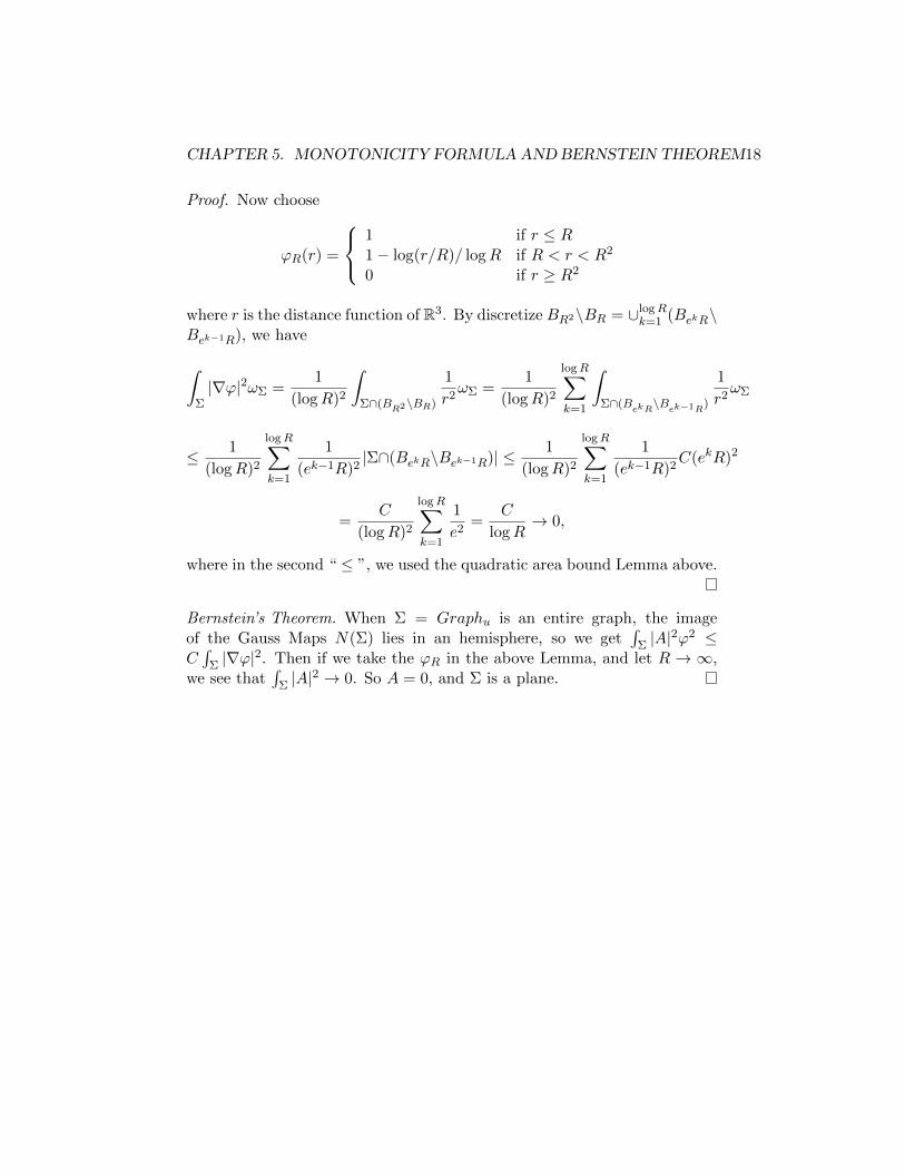
Proof. Now choose

ϕR(r) =

1 if r ≤ R1− log(r/R)/ logR if R < r < R2

0 if r ≥ R2

where r is the distance function of R3. By discretize BR2\BR = ∪logRk=1 (BekR\

Bek−1R), we have

∫Σ|∇ϕ|2ωΣ =

1

(logR)2

∫Σ∩(BR2\BR)

1

r2ωΣ =

1

(logR)2

logR∑k=1

∫Σ∩(B

ekR\B

ek−1R)

1

r2ωΣ

≤ 1

(logR)2

logR∑k=1

1

(ek−1R)2|Σ∩(BekR\Bek−1R)| ≤ 1

(logR)2

logR∑k=1

1

(ek−1R)2C(ekR)2

=C

(logR)2

logR∑k=1

1

e2=

C

logR→ 0,

where in the second “ ≤ ”, we used the quadratic area bound Lemma above.

Bernstein’s Theorem. When Σ = Graphu is an entire graph, the imageof the Gauss Maps N(Σ) lies in an hemisphere, so we get

∫Σ |A|

2ϕ2 ≤C∫

Σ |∇ϕ|2. Then if we take the ϕR in the above Lemma, and let R → ∞,

we see that∫

Σ |A|2 → 0. So A = 0, and Σ is a plane.

Chapter 6

Second variation andStability

6.1 Second Variation of Volume

Consider a minimal Σk ⊂Mn, i.e. ~H = 0. Given a vector field X on Σ, letFt be the geometric flow related to X, i.e.

F0 = id

d

dtFt(p)|t=0 = X(p), p ∈M

Theorem 6.1 (Second Variation Formula).

δ2Σ(X,X) :=d2

dt2|t=0Area(Σt) =

∫Σ

[|D⊥X|2−|〈 ~A,X〉|2−k∑i=1

RM (ei, X, ei, X)],

(6.1)where e1, · · · , ek is an orthonormal basis tangent to Σ, and X is compactsupported and normal on Si.

Proof. • F : Σ × (−ε, ε) → M , with x1, · · · , xk local coordinates onΣ, s.t. F (p, t) = Ft(p), p ∈ Σ. Then dvolt =

√detg(t)dx, where

gij(t) = 〈 ∂F∂xi, ∂F∂xj〉.

•d

dt

√detg(t) =

1

2gij gij

√detg(t)

19

CHAPTER 6. SECOND VARIATION AND STABILITY 20

•

d2

dt2

√detg(t) =

1

4(gij gij)

2√detg +

1

2gij gij

√detg +

1

2(gij gij)

√detg,

where gij = −gikgjlgkl.•

gij = 〈D ∂F∂t

∂F

∂xi,∂F

∂xj〉+ 〈 ∂F

∂xj, D ∂F

∂t

∂F

∂xi〉

= 〈D ∂F∂xi

∂F

∂t,∂F

∂xj〉+ 〈 ∂F

∂xj, D ∂F

∂xi

∂F

∂t〉

= −〈∂F∂t,D ∂F

∂xi

∂F

∂xj〉 − 〈D ∂F

∂xi

∂F

∂xj,∂F

∂t〉

= −〈 ~A(∂

∂xi,∂

∂xj), X〉.(When t = 0.)

So(gij gij)|t=0 = −2〈 ~H,X〉 = 0,

and(gij gij)|t=0 = −4|〈 ~A,X〉|2.

•

gij = 〈D ∂F∂tD ∂F

∂xi

∂F

∂t,∂F

∂xj〉+ 〈D ∂F

∂xj

∂F

∂t,D ∂F

∂t

∂F

∂xi〉

+ 〈D ∂F∂tD ∂F

∂xj

∂F

∂t,∂F

∂xi〉+ 〈D ∂F

∂xi

∂F

∂t,D ∂F

∂t

∂F

∂xj〉

= 〈RM (∂F

∂t,∂F

∂xi)∂F

∂t,∂F

∂xj〉+ 〈D ∂F

∂xiF ,

∂F

∂xj〉+ 〈D ∂F

∂xiX,D ∂F

∂xjX〉

+ 〈RM (∂F

∂t,∂F

∂xj)∂F

∂t,∂F

∂xi〉+ 〈D ∂F

∂xjF ,

∂F

∂xi〉+ 〈D ∂F

∂xjX,D ∂F

∂xiX〉

= −RM (X,∂

∂xi, X,

∂

∂xj) + 〈D ∂

∂xiF ,

∂

∂xj〉+ 〈D ∂

∂xiX,D ∂

∂xjX〉

−RM (X,∂

∂xj, X,

∂

∂xi) + 〈D ∂

∂xjF ,

∂

∂xi〉+ 〈D ∂

∂xjX,D ∂

∂xiX〉

So

(gij gij)|t=0 = −2gijRM (X,∂

∂xi, X,

∂

∂xj)+2divΣF+2|D⊥X|2+2gij〈DT

∂

∂xiX,DT

∂

∂xjX〉︸︷︷︸

=2|〈 ~A,X〉|2


• Combining all the above,

d2

dt2|t=0

√detg(t) = divΣF+|D⊥X|2−|〈 ~A,X〉|2−gijRM (X, ∂xi, X, ∂xj).

An integration on Σ finishes the proof.

Theorem 6.2. In the case Σn−1 ⊂Mn is a hyper surface and 2-sided(thereexist global unit normal ν), X = ϕν, with ϕ a function with compact support,then

δ2Σ(ϕ,ϕ) =

∫Σ

[|∇ϕ|2 − (|A|2 +RicM (ν, ν))ϕ2] (6.2)

Proof. We have

|D⊥X| = 〈D⊥X, ν〉 = 〈∇φν, ν〉+ 〈φD⊥v, v〉 = |∇φ|,

|〈A,X〉|2 = |φ|2|〈A, v〉|2 = φ2|A|2,n−1∑i=1

R(X, ei, X, ei) =n−1∑i=1

φ2R(ν, ei, ν, ei) = φ2Ric(ν, ν).

6.2 Jacobi operator and Stability

Definition 6.3 (Stability). Σ is stable if I(X,X) := δδΣ(X,X) ≥ 0, ∀Xnormal with compact support.

Corollary 6.4. If Ric ≥ 0, then there is no closed 2-sided stable minimalhypersurface.

Proof. Take φ = 1 in Theorem 6.2.

Corollary 6.5. If Σn−1 ⊂Mn is two-sided and stable minimal surface, thenRic(ν, ν) = 0 on Σ, where ν is normal on Σ. Moreover, Σ is total geodesic.

Proof. Take φ = 1.

Remark 6.6. The 2-side condition is essential. Since RP 2 → RP 3 isstable, but Ric 6= 0.

Proof.


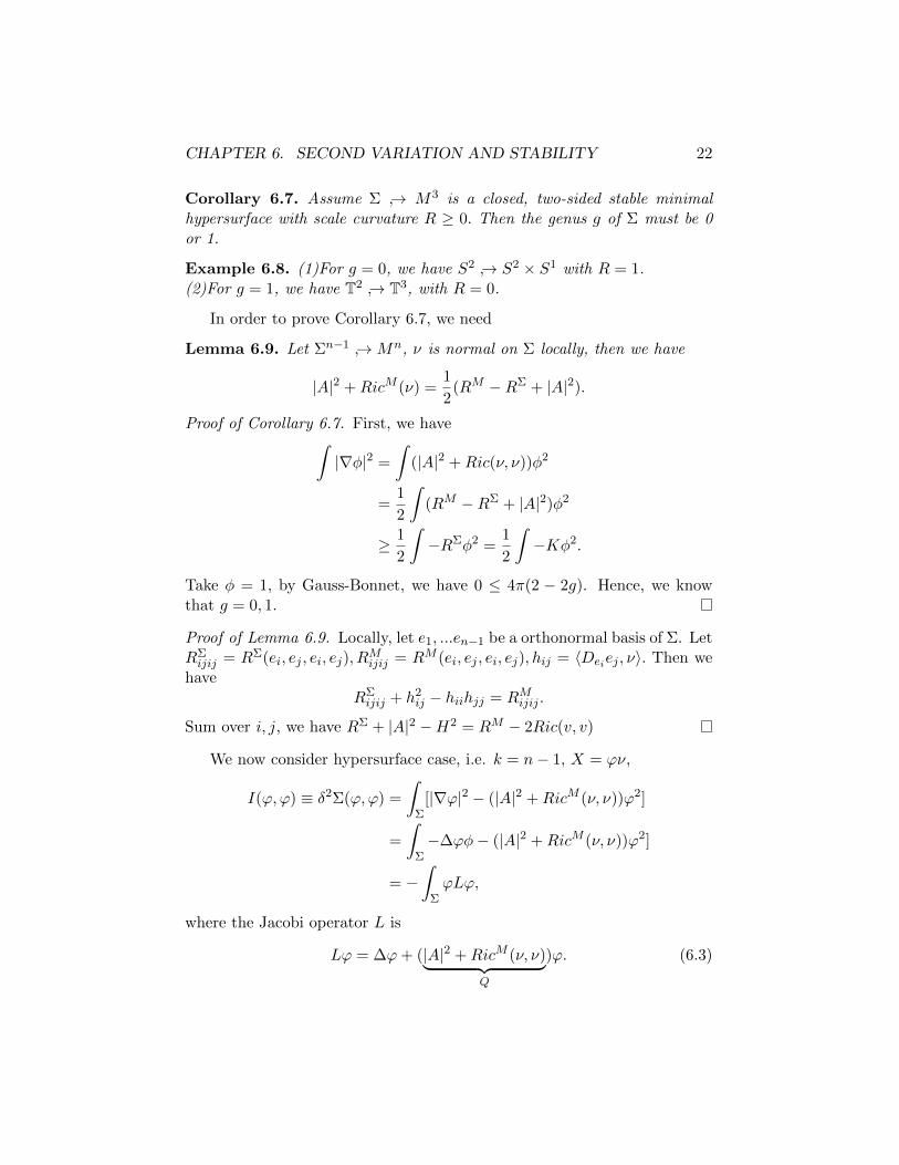
Corollary 6.7. Assume Σ → M3 is a closed, two-sided stable minimalhypersurface with scale curvature R ≥ 0. Then the genus g of Σ must be 0or 1.

Example 6.8. (1)For g = 0, we have S2 → S2 × S1 with R = 1.(2)For g = 1, we have T2 → T3, with R = 0.

In order to prove Corollary 6.7, we need

Lemma 6.9. Let Σn−1 →Mn, ν is normal on Σ locally, then we have

|A|2 +RicM (ν) =1

2(RM −RΣ + |A|2).

Proof of Corollary 6.7. First, we have∫|∇φ|2 =

∫(|A|2 +Ric(ν, ν))φ2

=1

2

∫(RM −RΣ + |A|2)φ2

≥ 1

2

∫−RΣφ2 =

1

2

∫−Kφ2.

Take φ = 1, by Gauss-Bonnet, we have 0 ≤ 4π(2 − 2g). Hence, we knowthat g = 0, 1.

Proof of Lemma 6.9. Locally, let e1, ...en−1 be a orthonormal basis of Σ. LetRΣijij = RΣ(ei, ej , ei, ej), R

Mijij = RM (ei, ej , ei, ej), hij = 〈Deiej , ν〉. Then we

haveRΣijij + h2

ij − hiihjj = RMijij .

Sum over i, j, we have RΣ + |A|2 −H2 = RM − 2Ric(v, v)

We now consider hypersurface case, i.e. k = n− 1, X = ϕν,

I(ϕ,ϕ) ≡ δ2Σ(ϕ,ϕ) =

∫Σ

[|∇ϕ|2 − (|A|2 +RicM (ν, ν))ϕ2]

=

∫Σ−∆ϕφ− (|A|2 +RicM (ν, ν))ϕ2]

= −∫

ΣϕLϕ,

where the Jacobi operator L is

Lϕ = ∆ϕ+ (|A|2 +RicM (ν, ν)︸︷︷︸Q

)ϕ. (6.3)


When boundary exists (Σ, ∂Σ), L has discrete eigenvalues λj and eigen-functions uj with Dirichlet condition, i.e.

Luj + λjuj = 0, in Σ

uj = 0, on ∂Σ

andλ1 < λ2 ≤ λ3 ≤ · · · ,

with λn → +∞.

Definition 6.10. Morse Index of Σ is defined as the number of negativeeigenvalues counted with multiplicity.

Proposition 6.11. (1)λ1 has multiplicity 1;(2)If u1 is an eigenfunction of λ1, u1 does not change sign.

Proof. We just prove (2) Here. By the variational characterization, u1

minimizes I(ϕ,ϕ) among all ϕ with ϕ ≡ 0 on ∂Σ and∫

Σ ϕ2 = 1. Since

|(|ϕ|, |ϕ|) = I(ϕ,ϕ), if u1 is the first eigenfunction, so is |u1|. So u1 = |u1|,or there is a contradiction to u1 ∈ C∞. The fact that u1 does not changesign shows that the dimension of the eigen space of λ1 is 1, or we can alwaysform some eigenfunction changing sign.

Definition 6.12. When Σ is non-compact, then

Ind(Σ) = limi→∞

Ind(Ωi),

where Ωi∞i=1 is an open exhaustion of Σ, i.e. Σ = ∪∞i=1Ωi, Ωi ⊂ Ωi+1, with∂Ωi smooth and compact.

Remark 6.13. In fact, the definition is independent of the exhaustion, sayΩi and Ωi.

Proof. First, we have λk = infλ(V ) : V ⊂ C∞c (Ω), dim(V ) = k, whereλ(V ) = sup−

∫Lff : f ∈ V,

∫|f |2 = 1(cf. [1] section 4.5). By this we can

see Ind(Ω) is non decreasing when Ω is expanding (since C∞c (Ω) ⊂ C∞c (Ω′)when Ω ⊂ Ω′), so we can always embed Ωi ⊂ Ωi′ for i′ i, so Ind(Ωi) ≤Ind(Ωi′), and limi→∞ Ind(Ωi) ≤ limi′→∞ Ind(Ωi′), and vise versa.

When Σ is open:

λ1(Σ) = limi→∞

λ1(Ωi) ∈ [−∞, λ1(Ω1)),

Σ is stable if λ1(Σ) ≥ 0, or equivalently λ1(Ω) ≥ 0 for all Ω ⊂ Σ.


Remark 6.14. By the variational characterization, λ1(Ω) is strictly de-creasing as Ω is expanding, so we can argue as above to show the well-definedness of λ1(Σ).

Chapter 7

Additional Topics inStability I

• Let Σ2 ⊂M3 be a closed, two-sided stable minimal hypersurface withpositive scale curvature R. In the proof Corollary 6.7, we know that ifthe scale curvature R > 0, we must have Σ = (S2, g). Hence, we havethe following positive mass theorem

Theorem 7.1. There is no positive scale metric on T3.

Proof. By an Theorem 4.1 in [6] given by Schoen-Yau, there exists anarea-minimizing immersion u : T2 → T3. If there exists a positivescale metric on T3, then we know from the proof of Corollary 6.7 thatthe genus of u(T) must be 0, which is a contradiction.

• We now focus on the 3-manifold M , which admits a scale curvatureR ≥ 6 in the following. Marques-Neves(2013) and Song(2015) (???Not sure) show that if there exists a least area minimal surface ofΣ ⊂M , then Area(Σ) ≤ 4π. The equality holds iff M is the standard3-sphere S3.(1)We would like to study the stable 1-sided minimal surfaces first.An example is that RP 2 → RP 3.Let Σ2 ⊂ M3 be a stable 1-side minimal surface, X be a normal fieldon Σ with compact support. Moreover, let π : Σ 7→ Σ be a 2-cover ofΣ, ν be a unit normal vector field of Σ →M3, i : Σ 7→ Σ be the decktransformation. Then we have(a)ν i = −ν.

25

CHAPTER 7. ADDITIONAL TOPICS IN STABILITY I 26

(b)Let X = X π, then X i = X.Hence, if we assume X = φν, then we have φ i = −φ.Since Σ is stable, for any φ ∈ C∞(M), s.t. φ i = φ, we have∫

Σ|∇φ|2 ≥

∫Σ

(Ric(ν, ν) + |A|2)φ2 (7.1)

Moreover, we have a conformal map F : Σ 7→ S2(1) → R3, s.t. degF ≤g(Σ) + 1, F i = F, where g(Σ) is the genus of Σ. Assume F =(f1, f2, f3), then∫

Σ(Ric(ν, ν) + |A|2) =

3∑i=1

∫Σ

(Ric(ν, ν) + |A|2)f2i

≤∑∫

Σ|∇fi|2 =

∫Σ|∇F |2

= 2deg(F )Area(S)(integration by substitution)

= 8πdeg(F ) ≤ 8π(g(Σ) + 1).

(7.2)

while∫ΣRic(ν, ν) + |A|2 =

1

2

∫ΣRM −RΣ + |A|2

≥ 1

2

∫Σ

6−K

=

∫Σ

6−K = 6Area(Σ)− 4π(1− g)

(7.3)

By (7.2) and (7.3), we have Area(Σ) ≤ 2π, whenever g = 0 or 1.

(2)We then consider the 2-sided minimal surface Σ ⊂M , with ind(Σ) =1, i.e., there exists one and only one negative eigenvalue λ1 for Jacobioperator L. Let u1 be the eigenvector for λ1, then for any φ ⊥ u1, wehave ∫

(Ric(ν, ν) + |A|2)φ2 ≤∫|∇φ|2. (7.4)

Since φ lies in a subspace that generated by nonnegative eigenvector.Moreover, there exist holomorphic map F : Σ 7→ S2, s.t. degF ≤[3g+1

4 ], where [x] is the integer-valued function. Notice that

w =

∫Σu1F ∈ B3,

CHAPTER 7. ADDITIONAL TOPICS IN STABILITY I 27

where B3 = x ∈ R3 : |x| < 1. For any v ∈ B3, there exist conformalfunction F : B3 7→ B3, s.t. Fv(v) = 0. Let G = Fw F , we have∫

Σu1G = 0. (7.5)

Let G = (g1, g2, g3), by (7.4) and (7.5), we have∫Lgigi ≥ 0.

Hence,∫Σ

(Ric(ν, ν) + |A|2 ≤∫

Σ|∇G|2 ≤ degGArea(S2) ≤ 4π[

3g + 1

4]

while∫ΣRic(ν, ν) + |A|2 =

1

2

∫ΣRM −RΣ + |A|2

≥ 1

2

∫Σ

6−K

=1

2

∫Σ

6−K = 3Area(Σ)− 2π(1− g),

(7.6)

we have 3Area(Σ) ≤ 2π(1− g) + 4π[3g+14 ].

Moreover, it’s straightforward to check that Ric(ν, ν) + |A|2 ≥ −2K.So we have 4π(g − 1) ≤ 4π[3g+1

4 ]. Consequently, g ≤ 3.

• We have the following estimate:

Theorem 7.2 (Schoen-Yau). Let (Σ2, ∂Σ) → (M3, g) be a stable min-imal surface. Moreover, the scale curvature Rg of M has a positivelower bound Λ, i.e. Rg ≥ Λ > 0. Then, we have rinf(Σ, ∂Σ) ≤ C√

Λfor

some positive constant C, where rinf = maxp∈Σ dist(p, ∂Σ).

Corollary 7.3. Let (M, g) be a noncompact Riemannian manifoldwith Rg ≥ Λ > 0, then there is no complete stable minimal surface in(M3, g).

Chapter 8

Criterion for stability

Theorem 8.1. Let Σ ⊂M be a 2-sided minimal surface, Σ is stable iff(1)when Σ closed, there exist u > 0, s.t. LΣu ≤ 0.(2)when Σ is complete and noncomplete, there exist u > 0, s.t. LΣu = 0.

Remark 8.2. This can be viewed as an infinitesimal version of the Calibra-tion argument i.e. using foliation of minimal surfaces.

Corollary 8.3. Σ ⊂ M is 2-sided minimal surface, Σ is stable, then forany covering map π : Σ 7→ Σ, if Σ ⊂M , then Σ is also 2-sided and stable.

Proof. Let u > 0 satisfy the condition in Theorem 8.1, then we have

LΣ(u π) =

≤ 0,when Σ is compact,

= 0,when Σ is noncompact.

Remark 8.4. The ”2-sided” condition is essential, consider RP 2 → RP 3

is stable, but S2 → RP 3 is not.

Proof for Theorem 8.1. ⇐=: Since Lu = ∆Σu+Qu ≤ 0, let w = log u(u >0), we have

∆w =∆u

u− |∇w|2 ≤ −Q− |∇w|2.

Then ∀ϕ compactly supported,∫Σϕ2(∆w +Q) ≤ −

∫Σϕ2|∇w|2.

28

CHAPTER 8. CRITERION FOR STABILITY 29

Using integration by part formula,∫ΣQϕ2 ≤

∫2ϕ〈∇ϕ,∇w〉 − |∇w|2ϕ2 ≤

∫2|ϕ||∇ϕ||∇w| − |∇w|2ϕ2

≤∫|∇ϕ|2 + ϕ2|∇w|2 − |∇w|2ϕ2 ≤

∫Σ|∇ϕ|2.

Hence we have the stability inequality for Σ.=⇒(1) Assume Σ is compact, then ∃u > 0, which is the first eigenfunction,such that λ1(Σ) ≥ 0, so

Lu = −λ1u ≤ 0.

(2) Assume Σ is non-compact and stable, then Σ has an exhaustionΣ = ∪∞i=1Ωi, and λ1(Ωi) > 0 for all i. Now by elementary elliptic PDE,∀ψ ∈ C(∂Ωi), ∃!u in Ωi, such that

Lui = 0, in Ωi,

ui = ψ, on ∂Ωi.

Claim: λ1(Ωi) > 0 =⇒ if ψ > 0, then u > 0.Otherwise, if u ≤ 0, then Ωu≤0 has eigenvalue equals 0, since u is then aDirichlet eigenfunction on Ωu≤0 with 0 boundary values, extend u by 0 tou ∈W 1,2(Ωi), let w be the λ1(Ωi) eigenfunction of L, then we have

0 < λ1(Ω) =

∫Ωi

(−Lw)w∫Ωi|w|2

= infv ∈W 1,2(Ωi) :

∫Ωi

(−Lv)v∫Ωi|v|2

≤∫

Ωi(−Lu)u∫Ωi|u|2

= 0,

(8.1)which is a contradiction.

Now we can solve the boundary value problem for ui > 0:Lui = 0 in Ωi,

u = 1 on ∂Ωi.

Fix p ∈ Ω1, then consider the normalized sequence uiui(p)∞i=1,

Claim: Let ui = uiui(p)

, then there exists a subsequence i′ →∞, u ∈ C∞(Σ),such that

ui′ → u in C2 on any compact subset of Σ,

andLu = 0.

Proof of Claim: Fix any compact subset K ⊂ Σ, then when i big enough,K ⊂⊂ Ωi. Hence, we may assume K ⊂⊂ Ωi for all i > 0. Fix Ω,Ω′ s.t.


K ⊂⊂ Ω ⊂⊂ Ω′ ⊂⊂ Ω1.By Hanack inequality (cf. Theorem 4.3.3 [2]), we have

supx∈Ω′|ui(x)| ≤ C(n,Ω′,Ω1) inf

x∈Ωi|ui| ≤ C(n,Ω′,Ω1)u(p) = C(n,Ω′,Ω1).

By a standard regularity theorem of EPDE, we could see that ui ∈ C∞(Ω1).Hence, by Gradient Estimate of EPDE (cf. Proposition 2.3.2 in [2]), we have

supx∈Ω|Dui(x)| ≤ C(n,Ω,Ω′) sup

x∈Ω′|ui(x)| ≤ C(n,Ω,Ω′,Ω1).

By Schauder Estimate, we have

‖ ui ‖C3(K)≤ C(n,K,Ω1).

The claim follows from standard application of Ascoli.The limit u is a positive solution of Lu = 0.

Definition 8.5 (Convergence in the C∞ sense). We say a sequence of min-imal surface Σn−1 ⊂ Rn converge to Σ in the sense of C∞, if for any p ∈ Σ,there exist r > 0, s.t.

Σi ∩Br(p) = Graph of ui over TpΣ for i large enough,

and ui → u in C∞ topology, where u is a function s.t. Σ is a graph of uover TpΣ.

Example 8.6. (1)Let Σ → Mn be the C∞ embedding hypersurface. Forany p ∈ Σ, ri → 0, Σp,ri = Σ−p

ri→ TpΣ in the sense of C∞.

(2)Let C be the Catenoid, then λiC → 2R in C∞ sense, except for 0.

Theorem 8.7 (L. Simon). If Σi → Σ in C∞ sense, then there exists u 6= 0,s.t. LΣu = 0. If Σ lie in one side of Σ, we could find u > 0, s.t. LΣu = 0.

Remark 8.8. The Proof of Theorem 8.7 is similar to Theorem 8.1.

Proposition 8.9. 1. Let Σn−1 ⊂ Rn be a 2-sided minimal surface, and ifthe Gauss image G(Σ) ⊂ Sn−1

+ , then Σ is stable;2. Let Σ2 ⊂ R3 be a 2-sided minimal surface, and if G(Σ) ⊂ Uopen ⊂ S2,with µ1(U) ≥ 1, where µ1(U) is the Dirichlet eigenvalue of ∆S2 on U , thenΣ is stable. In perticular, µ1(U) ≥ 1 is true if the area |U | ≤ 2π.


Proof. 1. Let e ∈ Rn be the direction vector to the north pole, and letu = e·ν, where ν is the normal vector field of Σ, since the parallel translationin the e direction does not change the area of Σ, we have Lu = 0. SinceG(Σ) ⊂ Sn−1

+ ⇐⇒ e · ν > 0, so u > 0, hence Σ is stable.2. µ1(U) ≥ 1 =⇒ ∃v > 0 on U such that

∆S2v = µi(U)v ≤ −v, in U,v = 0, on U.

Let u = v G, where G is the Gauss Map. By Lemma 5.9, G : Σ→ S2 is aconformal map, so

∆Σu = |A|2(∆S2v) G ≤ −|A|2u,

i.e. Lu ≤ 0, hence Σ is stable. (In fact, on 2-dimension, the Jacobi operatorL = G∗(∆S2 + 1).)

Chapter 9

The Generalized BernsteinTheorem

This chapter, we are going to prove:

Theorem 9.1 (The Generalized Bernstein Theorem). Any complete non-compact 2-sided stable minimal immersion Σ2 ⊂ R3 is a plane.

9.1 Bochner Technique

In this section, we will use Bochner Technique to prove:

Theorem 9.2 (Vanishing of Harmonic 1-Forms). If Σn−1 ⊂ Rn is a com-plete, stable and 2-sided minimal surface, then any L2 harmonic 1-form onΣ vanishes.

Let (Σk, g) be a Riemannian manifold, and e1, · · · , ek an o.n. frame,with θ1, · · · , θk the dual frame. Denote

(∇ejα) =∑i

αi,jθi,

∇ei(∇α) =∑i,j

αi,jkθi ⊗ θj ;

then∇α =

∑i,j

αi,jθi ⊗ θj , ∇2α =

∑i,j,k

αi,jkθi ⊗ θj ⊗ θk.

Ricci Formula:αi,jk − αi,kj =

∑p αpR

Σpijk.

32

CHAPTER 9. THE GENERALIZED BERNSTEIN THEOREM 33

Definition 9.3. α is harmonic if dα = 0 and δα = 0(i.e. αi,j = αj,i and∑i αi,i = 0).

Bochner Formula: If α is harmonic, then

∆α = Ric(α], ·),

where α] the vector field dual to α, and ∆α =∑

i,j αi,jjθi is the rough laplacian.

Proof. ∑j

αi,jj =∑j

αj,ij =∑j

αj,ji︸︷︷︸=0

+∑p,j

αpRΣpjij =

∑p

αpRicΣpi.

Hence we have:

12∆|α|2 = 〈α,∆α〉+ |∇α|2 = Ric(α], α]) + |∇α|2 .

In the case Σn−1 ⊂ Rn is minimal, RΣijkl = hikhjl− hilhjk under the o.n.

frame ei by the Gauss equation, hence

RicΣik =

∑j

RΣijkj = −

∑j

hijhjk, (∑j

hjj = 0).

=⇒ 1

2∆|α|2 = |∇α|2+

∑ij

RicΣijαiαj = |∇α|2−

∑i

(∑j

hijαj)2 ≥ |∇α|2−|A|2|α|2.

Plug in 12∆|α|2 = |α|∆|α|+

∣∣∇|α|∣∣2,

|α|(∆|α|+ |A|2|α|︸︷︷︸L|α|

) ≥ |∇α|2 −∣∣∇|α|∣∣2 ≥ c(n)

∣∣∇|α|∣∣2,where Lu = ∆u + |A|2u is the stability operator, and c(n) a constant de-pending only on n.

In general, choose the o.n. basis e1, · · · , ek such that under this basisα1 = |α| and αj = 0 for j = 2, · · · , k, then

|∇α|2 −∣∣∇|α|∣∣2 =

∑ij

α2i,j −

∑j(∑

i αiαi,j)2

|α|2=∑i,j

α2i,j −

∑j

α21,j


=∑i>1,j

α2i,j ≥

k∑i=2

α2i,i +

k∑i=2

α2i,1 ≥

1

k − 1(k∑i=2

αi,i︸︷︷︸=−α1,1

)2 +k∑i=2

α21,i

≥ 1

k − 1[α2

1,1 +k∑i=2

α21,i] =

1

k − 1

∣∣∇|α|∣∣2.Proof of Theorem 9.2. 2-sided and stability means that −

∫Σ ϕLϕ ≥ 0 for

any ϕ compactly supported. So ∀ϕ compactly supported

−∫

Σϕ|α|L(ϕ|α|) ≥ 0,

i.e. ∫Σϕ|α|(∆(ϕ|α|)︸︷︷︸

I

+|A|2ϕ|α|) ≤ 0,

where

I =

∫Σϕ|α|(ϕ∆|α|+2〈∇ϕ,∇|α|〉+|α|∆ϕ) =

∫Σϕ2|α|∆|α|+1

2〈∇ϕ2,∇|α|2〉+|α|2ϕ∆ϕ

≤∫

Σϕ2|α|∆|α| −

∫Σ

1

2∆(ϕ2)|α|2 +

∫Σ|α|2ϕ∆ϕ

=

∫Σϕ2|α|∆|α| − (ϕ∆ϕ+ |∇ϕ|2)|α|2 + |α|2ϕ∆ϕ

=

∫Σϕ2|α|∆|α| − |∇ϕ|2|α|2.

Plug into the above ∫Σϕ2|α|L(|α|) ≤

∫Σ|∇ϕ|2|α|2.

Now by taking ϕ = ϕR to be cutoff functions on geodesic disk, and let-ting R → ∞, the righthand side of the above inequality is zero, hence by|α|L(|α|) ≥ c(n)

∣∣∇|α|∣∣ proved above,

c(n)

∫Σ

∣∣∇|α|∣∣2 ≤ ∫Σ|α|L(|α|) = 0,

which means that |α| is a constant, and hence is 0 since the area of Σ is ∞by the monotonicity |Bσ(p)| ≥ wkσk.


9.2 Proof of Generalized Bernstein Theorem

First, it’s easy to see that:

Lemma 9.4. Let (Σ2k, g) be 2k-dimensional manifolds, for any ω ∈ ΩkΣ,the L2 norm of ω is comformally invariant.

Lemma 9.5. If α is harmonic in (Σ2, g), then α is also harmonic in (Σ, ρg),for any smooth function ρ > 0.

Proof. We notice that dα = 0,

δρgα = ρ−2δgα = 0.

Proposition 9.6. Σ ∼= D2 cannot be conformally imersed into R3 as acomplete noncompact 2-sided stable minimal surface.

Proof. Let (R3, δ) be standard Euclidean space, and i : Σ 7→ D be the con-formal map. By Lemma 9.4 and Lemma 9.5, we could see that L2 harmonic1-form on (Σ, i ∗ δ) is one to one correspond to L2 harmonic form on (D, δ).

Since there are many harmonic 1-forms on D by just taking df where fis harmonic functions, so it is a contradiction to the Theorem 9.2.

Proof of Theorem 9.1. (Σ, g) is an oriented Riemann surface, where g is therestriction metric. If z = x + iy then g = λ2(dx2 + dy2) locally. So Σ hasa complex striation. Let Σ be the universal cover of Σ, then Σ is a simplyconnected non-compact Riemann surface, hence by uniformization theoremof Riemann surface,

Σ '

C, the complex plane,D, the unit disk.

By Proposition 9.6, second situation could not happen.Hence, Σ ' C, then let F : C → R3, where F = i π is given by the

composition of the minimal immersion i : Σ → R3 with the covering mapπ : C ' Σ→ Σ. Since i is harmonic, and the harmonic?property is preservedunder the conformal change Σ ' C, we know that F is both conformal andharmonic, i.e. ∆CF = 0. Since Σ is stable and 2-sided, Σ is also stable and2-sided, =⇒ ∃u > 0, such that Lu = ∆Σu + |A|2u = 0 on Σ. So ∆Σu ≤ 0,hence ∆C(u F ) ≤ 0. So u F is a super-harmonic function. Since C hasquadratic area growth,together with the fact that u F > 0, we know thatu F = 0, and hence |A|2 = 0 by the following Proposition.


Definition 9.7. A Riemannian manifold Σk is called parabolic if everypositive super-harmonic function is constant.

Proposition 9.8. If h : Σ → R1+ is a proper Lipschitz function |∇h| ≤ c,

and if |Σa| ≤ ca2 for some c > 0, where Σa = p ∈ Σ : h(p) ≤ a, then Σis parabolic.

Proof. Take a positive super-harmonic function u, i.e. ∆u ≤ 0 and u > 0.Take w = log u, then

∆w =∆u

u− |∇w|2 ≤ −|∇w|2.

Take ϕ a compactly supported function,∫Σϕ2|∇w|2 ≤ −

∫Σ

∆wϕ2 =

∫2〈∇w,ϕ〉ϕ

≤ 2

∫|ϕ||∇w||∇ϕ| ≤ ε

∫ϕ2|∇w|2 +

1

ε

∫|∇ϕ|2.

Taking ε = 12 , then ∫

Σϕ2|∇w|2 ≤ 4

∫Σ|∇ϕ|2.

By taking h = distΣ(·, p), we know that Σ has more than quadratic areagrowth, so we can take ϕ = ϕR as in Lemma 5.13, and use the same loga-rithmic cut-off trick, to get

∫Σ |∇ϕR|

2 → 0, and ϕR → 1. So |∇w| = 0, andw hence u is a constant.

Chapter 10

Curvature Estimate

Theorem 10.1. Let Σn−11 ,Σn−1

2 be two connected, imbedded minimal hy-persurfaces of Rn, s.t.

Σi ∩Br(0) 6= ∅, Br(0) ∩ ∂Σi = ∅.

Moreover, we assume Σ1 separate Br(0), and Σ2 lie in one side of Σ1, i.e.

Br(0)Σ = U1 ∪ U2,Σ2 ∩Br(0) ⊂ U1,

where Ui is open and connected. Then, either Σ1 ∩ Σ2 = ∅ or Σ1 = Σ2.

Proof. Assume p ∈ Σ1 ∩ Σ2, then locally, they can be written as graphs ofu1, u2, s.t.

(δij −uαi u

αj

1 + |∇uα|)uαij = 0, α = 1, 2.

Substract the two equations, we have

δij(u1ij − u2

ij) + bi(u1 − u2)i + c(u1 − u2) = 0,

for some bi, c. Hence by maximal principle, u1 = u2 locally.

Let Σn−1 → Rn be a immersed minimal hypersurface, 0 ∈ Σ, let

Lr = Σ ∩Br(0) 6= ∅, ∂Σ ∩Br(0) = ∅,

we want to prove

|A|2(x) ≤ C

d2(x, ∂Br(0)).

37

CHAPTER 10. CURVATURE ESTIMATE 38

By a suitable dilation and translation, we just need to prove

|A|2(0) ≤ C.

Let e1, · · · , en−1 be local o.n. frames on Σ, and denote hij,klm by thecovariant derivatives of the second fundamental form h on Σ. The roughlaplacian for h is defined as

∆hij =

n−1∑k=1

hij,kk.

Proposition 10.2.

∆hij + |A|2hij = 0, 0 ≤ i, j ≤ n− 1 (10.1)

Proof. Firstly we have the Ricci identity:

hij,kl − hij,lk =∑p

hpjRpikl +∑p

hipRpjkl,

Gauss Equation:RΣijkl = hikhjl − hilhjk,

and Codazzi equation:hij,k = hik,j .

Using the Eistein summation, we have

∆hij = hij,kk = hik,jk = hik,kj︸︷︷︸=hkk,ij=0

+hpkRΣpijk + hipR

Σpkjk

= hpk(hpjhik − hpkhij) + hip(hpj hkk︸︷︷︸=0

−hpkhkj)

= −|A|2hij + (hikhkphpj − hipHpkhkj︸︷︷︸=0

).

So we finished the proof.

Now recall that the stability operator is Lϕ = ∆ϕ+ |A|2ϕ.

Proposition 10.3.

|A|(L|A|) ≥ 2

n− 1

∣∣∇|A|∣∣2. (10.2)

CHAPTER 10. CURVATURE ESTIMATE 39

Proof. By the Bochner Formula,

1

2∆|A|2 = |∇A|2 + 〈A,∆A〉 = |∇A|2 − |A|4.

While 12∆|A|2 = |A|∆|A|+ |∇|A||2,

|A|L(|A|) = |∇A|2 −∣∣∇|A|∣∣2 =

∑i,j,k

h2ij,k −

∑k(∑

ij hijhij,k)2

|A|2. (10.3)

In an o.n. eigenbasis e1, · · · , en−1 of h, hij = λiδij , so

∣∣∇|A|∣∣2 =

∑k(∑

i λihii,k)2

|A|2≤∑i,k

h2ii,k =

∑i 6=k

h2ii,k +

∑i

h2ii,i

=∑i 6=k

h2ii,k +

∑i

(−∑j 6=i

hjj,i)2 ≤

∑i 6=k

h2ii,k + (n− 2)

∑i 6=j

h2jj,i

= (n− 1)∑i 6=k

h2ii,k =

n− 1

2(∑i 6=k

h2ik,i +

∑i 6=k

hki,i).

So

(1 +2

n− 1)∣∣∇|A|∣∣2 ≤∑

i,k

h2ii,k +

∑i 6=k

h2ik,i +

∑i 6=k

h2ki,i ≤

∑i,j,k

h2ij,k = |∇A|2.

So we finished the proof.

Chapter 11

Choi-Schoen’s Theorem

Theorem 11.1 (Choi-Schoen [4]). Suppose Σ2 ⊂M3 is a minimal surface.Assume 0 ∈ Σ2, and ∂Σ ∩ Br0(0) = ∅. Moreover, there exists ε, ρ > 0(depending only on M), such that

∫Σ∩Br0

|A|2 < ε, then

d2(x, ∂Bρ(0))|A|2(x) ≤ δ.

Proof. Let us give a proof when M3 = R3, and the general cases follow bythe fact that M3 is locally near R3 when ρ is small enough. Assume δ = 1and

F (x) = d2(x, ∂Bρ(0))|A|2(x),

Since F |∂Br0 = 0, then ∃x0 ∈ Bρ, such that F (x0) = maxBr0 F (x).Need to show: F (x0) ≤ 1.

Suppose otherwise F (x0) > 1, let δ = ρ−r(y0)2 , then

• supBδ(y) |A|2 ≤ 4|A|2(x0).

This is because d2(x, ∂Bρ(0))|A|2(x) ≤ 4d2(x0, ∂Bρ(0))|A|2(x0), hence

|A|2(x) ≤ (d2(x0,∂Bρ(0))d2(x,∂Bρ(0))

)2|A|2(x0) ≤ (d2(x0,∂Bδ(x0))d2(x,∂Bδ(x0))

)2|A|2(x0) ≤ 4|A|2(x0).

• (2δ)2|A|2(x0) = F (x0) > 1 =⇒ δ2|A|2(x0) > 1/4.

Let δ0 = 1|A|(x0) , hence δ2 ≥ 1

4δ20 =⇒ δ0/2 < δ. So Bδ0/2(x0) ⊂ Bδ(x0). Let

Σδ0 =2

δ0(Σ− x0),

=⇒

supB1|AΣδ0

|2 = 4|AΣδ0|2 = δ2

0 |A|2(x0) = 1,∫B1|AΣδ0

|2 ≤ ε.

40

CHAPTER 11. CHOI-SCHOEN’S THEOREM 41

By Simon’s equation, let A = AΣδ0, on B1, we have

∆|A|2 = 2(|∇A|2 − |A|4) ≥ −2|A|4 ≥ −2|A|2

Hence by mean value property of subsolution of EPDE, we have |A(0)|2 ≤c∫

Σ∩B1|A|2 ≤ cε, which is a contradiction.

Corollary 11.2. Assume Σ2 ⊂ R3 is stable and 2-sided with quadratic areagrowth, i.e. Area(Σ ∩Br0) ≤ cr2

0, then

supΣ∩Br0/2

|A|2 ≤ cr−20 .

Proof. By stability, we have∫

Σ |A|2ϕ2 ≤

∫Σ |∇ϕ|

2. Since Σ has quadraticarea growth, we can use the logarithmic cutoff trick to get,∫

Σ∩Br0/k|A|2 ≤ C

log k, k 1.

So for k large enough, we have∫

Σ∩Br1 (y) |A|2 < ε, where r1 = r0/k, hence

|A|2(y) ≤ cr−21 ≤ c′r−2

0 , c′ = kc.

Lemma 11.3 (Generalized Monotone formula). Let Σk ⊂ Rn be a minimalsurface, ∂Σ ∩Bρ(0) = ∅, f : Σ 7→ R is smooth, then∫

Σ∩Bt fdvol

tk−∫

Σ∩Bs fdvol

sk

=

∫Σ∩(Bt\Bs)

f|x⊥|2

|x|k+2dvol +

1

2

∫ t

s

1

τk+1

∫Σ∩Bτ

(τ2 − |x|2)∆Σfdvoldτ,

where 0 < s < t, and x⊥ is the projection of x to the normal part of TxΣ.

Proof. First, we have∫Σ∩Bt

div(fx)dvolΣ =

∫∂(Σ∩Bt)

fx · ndσ =

∫∂(Σ∩Bt)

f |xT |dσ, (11.1)

where n = xT

|xT | is exterior normal vector field on ∂(Σ ∩Bt). While∫Σ∩Bt

div(fx)dvolΣ =

∫Σ∩Bt

∇f · xdvolΣ +

∫Σ∩Bt

fdiv(x)dvolΣ

=

∫Σ∩Bt

∇f · xdvolΣ +

∫Σ∩Bt

kfdvolΣ = I +

∫Σ∩Bt

kfdvolΣ.

(11.2)


We have estimate

I =

∫Σ∩Bt

∇f∇(|x|2

2)dvolΣ

=

∫Σ∩Bt

div(|x|2

2f)− |x|

2

2∆ΣfdvolΣ

=

∫∂(Σ∩Bt)

t2

2∇f · ndσ −

∫Σ∩Bt

|x|2

2∆ΣfdvolΣ

=

∫Σ∩Bt

(t2 − |x|2

2)∆ΣfdvolΣ

(11.3)

Take h(x) = |x|, then h ≤ t = Bt(0), then ∇h = xT

|x| For the right hand

side of (11.1), we have∫∂(Σ∩Bt)

f |xT |dσ = t

∫∂(Σ∩Bt)

f|xT ||x|

dσ

= td

dt

∫Σ∩Bt

f|xT ||x||∇h|dvol

= td

dt

∫Σ∩Bt

f|xT |2

|x|2

= td

dt

∫Σ∩Bt

f(1− |x⊥|2

|x|2)

= td

dt

∫Σ∩Bt

f −∫∂(Σ∩Bt)

f|x⊥|2

|xT |( By coarea formula)

(11.4)

Let F (t) =∫

Σ∩Bt f , by (11.1),(11.2),(11.3) and (11.4), we have

kF (t) = tF ′(t)−∫∂(Σ∩Bt)

f|x⊥|2

|xT |−∫

Σ∩Bt(t2 − |x|2

2)∆ΣfdvolΣ. (11.5)

The lemma then follows easily from the above ODE.

Lemma 11.4 (Mean Value Properity). If ∆Σf ≥ −cf in Σ ∩ B1, f > 0,then

f(0) ≤ c′∫

Σ∩B1

fdvolΣ.


Proof. Since ∆Σf ≥ −cf, (11.5) imply that

d

dt(t−kF (t)) = t−k−1(

∫∂(Σ∩Bt)

f|x⊥|2

|xT |+

∫Σ∩Bt

(t2 − |x|2

2)∆ΣfdvolΣ)

≥ − c2t−k+1

∫Σ∩Bt

fdvolΣ),

where F (t) =∫

Σ∩Bt f. Hence, we know that ect/2F (t) is increasing. Hence

f(0) = F (0) ≤ ec/2F (1) = ec/2∫

Σ∩B1f.

Chapter 12

Small Curvature impliesGraphical

Let us firstly give a technical lemma used in the argument of the abovesection.

Lemma 12.1. Σ2 ⊂ Rn is minimal. Assume that s2 supΣ |A|2 ≤ 116 . If

x0 ∈ Σ2 and distΣ(x0, ∂Σ) ≥ 2s (i.e. ∂Σ ∩B2s(x) = ∅), then

(i) BΣ2s(x0) is graphical over Tx0Σ of some function u, where BΣ

2s(x0) isthe geodesic ball of Σ, and |∇u| ≤ 1 and |Hessu| ≤ 1√

2s;

(ii) Let Σ′ be a connected component of Bs(x) ∩ Σ containing x0, thenΣ′ ⊂ BΣ

2s(x0).

Proof. Define d(x, y) = distSn−1(N(x), N(y)). Connect x to y ∈ Σ∩BΣ2s(x0)

by unit speed geodesic u : [0, r] 7→ Σ, s.t. u(0) = x0, u(r) = y. Then

d(x0, y) ≤∫ r

0|∇ΣN |dt ≤

∫ r

0|A|dt ≤

∫ r

0

1

4sdt <

1

2<π

4,

Hence Σ∩BΣ2s(x0) is contained in the graph of a function u over a subset of

Tx0Σ. Since

1√2≥ cos(d(x, y)) =< N(x0), N(y) >=

1√1 + |∇u(y)|2

,

we have |∇u(y)| ≤ 1. Since

A =1

1 + |∇u|2

ux1x1 ... ux1xn−1

.... . .

...uxn−1x1 ... uxn−1xn−1

, g =

1 + u2x1

... ux1uxn−1

.... . .

...uxn−1ux1 ... 1 + u2

xn−1

,

(12.1)

44

CHAPTER 12. SMALL CURVATURE IMPLIES GRAPHICAL 45

and|A|2 = AikAjlg

ijgkl,

we have|Hess(u)|2

(1 + |∇u|2)3≤ |A|2 ≤ 1

16s2,

Consequently,

|Hess(u)| ≤ 1√2s

Now we are going to prove:If y ∈ BΣ

2s(x0), then dRn(y, x0) > s. Therefore, Σ ∩BRn

s (x0) ⊂ BΣ2s(x0). Let

w : [0, 2s] 7→ Σ be a unital speed geodesic, and w(0) = x0, w(2s) = y. Since

|w(2s− w(0))| = |w(2s− u(0))||w′(0)| ≥ 〈w(2s)− u(0), w′(0)〉,

in order to prove |w(2s)− w(0))| > s, we just need to show

〈w(2s)− w(0), w′(0)〉 > s.

Let f(t) = 〈w(t)− w(0), w′(0)〉, we have f(0) = 0, f ′(0) = 1. Moreover

|f ′′(t)| = |〈u′′(t), u(0)〉| < 1

4s,

which mean

f(2s) = f(0) + 2f ′(0)s+1

2f ′′(ξ)(2s)2 > 2s− 1

4s(2s)2 = s.

Remark 12.2. Let U ⊂ R3, then Lc1,c2 = Σ ⊂ U, ∂Σ ∩ U = ∅, H(Σ) ≡0,maxU |AΣ| ≤ c1,Area(Σ) ≤ c2 is closed in C∞ topology.

Theorem 12.3. Let Σk ⊂ Rn be minimal. ∃ε = ε(n, k), if x ∈ Σ, ∂Σ ⊂∂Br0(x), and Θx(r0)− 1 < ε, then

supΣ∩Br0/2(x)

|A|2 ≤ r−20 .

Proof. • It suffices to assume that Θy(r1)− 1 < ε for all y ∈ Br1(x) ∩Σby the monotonicity formula 5.1.

CHAPTER 12. SMALL CURVATURE IMPLIES GRAPHICAL 46

• By rescaling the function (r1 − |y|)2|A|2(y) near the maximum pointas in the proof of Theorem 11.2, we can get another minimal surface,denoted still as Σ, such that 0 ∈ Σ, ∂Σ ⊂ ∂B1(0), |A|2 ≤ 1 on Σ, and|A|2(0) = 1

4 . Furthermore, by the small excess condition, |Σ∩B1(0)| ≤(1 + ε)ωk.

• This is not possible if ε ≤ ε0, for some ε0 > 0 small enough, by thefollowing argument.

• Compactness argument: consider the class

Cε = Σ : 0 ∈ Σ, ∂Σ ⊂ ∂B1(0), |A|2 ≤ 1, |A|2(0) =1

4, |Σ∩B1(0)| ≤ (1+ε)ωk.

If the curvature estimates is not true, then we can find a sequence Σi,with Σ ∩B1(0) ≤ (1 + 2−i)ωk. A subsequence Σi → Σ in Ck norm tosome minimal Σ∞, such that Σ∞ ∈ C0, i.e. |Σ∞ ∩B1(0)| = ωk, =⇒ Σis a disk, hence contradiction to the curvature assumption |A|2(0) = 1

4 .

Chapter 13

Schoen’s Curvature Estimate

Theorem 13.1. Assume that Σ2 is stable and 2-sided in R3. If x ∈ Σ anddist(x, ∂Σ) ≥ r0, then

Area(BΣr0(x0) ∩ Σ) ≤ 4π

3r2

0.

Proof. It suffices to assume π1(Σ) = 1, or we can pass to the universal

cover Σ of Σ, which is also stable and 2-sided. Since Area(BΣr0(x0) ∩ Σ) ≥

Area(BΣr0(x0) ∩ Σ), we can get the result. Let φ(x) = r0 − r(x, x0), then

φ ∈ C1c (Σ ∩BΣ

r0(x0)) and |∇φ| = 1 a.e.Moreover, by Stability, we have∫Σ∩BΣ

r0(x0)|A|2φ2dvolΣ ≤

∫Σ∩BΣ

r0(x0)|∇φ|2dvolΣ = Area(Σ ∩BΣ

r0(x0)).

(13.1)While∫

Σ∩BΣr0

(x0)|A|2φ2dvolΣ =

∫ r0

0

∫∂(Σ∩BΣ

r (x0))|A|2dσ|r0 − r|2dr (13.2)

Let f(r) =∫ r

0

∫ s0

∫∂(Σ∩BΣ

τ (x0)) |A|2dσdτds =

∫ r0

∫Σ∩BΣ

s (x0) |A|2dvolΣds, g(r) =

|r − r0|2. Then we have

f(0) = g(0) = 0, f ′(0) = g′(0) = 0.

Moreover,

LHS of (13.2) =

∫ r0

0f ′′(r)g(r)dr =

∫ r0

0f(r)g′′(r)

= 2

∫ r0

0

∫ r

0

∫Σ∩BΣ

τ (x0)|A|2dvolΣdτdr.

(13.3)

47

CHAPTER 13. SCHOEN’S CURVATURE ESTIMATE 48

Since

d

drLength(Σ ∩ ∂BΣ

r ) =

∫Σ∩∂BΣ

r (x0)kgdΣ = 2π −

∫Σ∩BΣ

r

KdvolΣ

= 2π +1

2

∫Σ∩BΣ

r (x0)|A|2dvolΣ,

we have

Area(Σ∩BΣr0) =

∫ r0

0Length(Σ∩∂BΣ

r )dr = πr20+

1

2

∫ r0

0

∫Σ∩BΣ

r (x0)|A|2dvolΣdr.

Combine with (13.1), (13.2) and (13.3), we have

Area(Σ ∩BΣr0) <

4

3πr2

0.

Hence, by Corollary 11.2, we have

Corollary 13.2. Let Σ2 ⊂ R3 be a minimal surface, x0 ∈ Σ, and ∂Σ ∩BR3

r0 (x0) = ∅. If Σ is stable and two-sided, then

supΣ∩BR3

r0(x0)

|A|2 ≤ C/r20.

Theorem 13.3. If p < 2 +√

2n−1 , then ∀φ ∈ C1

c (Br0(x0) ∩ Σ), we have∫Br0 (x0)∩Σ

|A|2pφ2p ≤ C(p)

∫Σ|∇φ|2p.

Proof. First, we claim:

2

n− 1

∫Σ

∣∣∇|A|∣∣2ϕ2 ≤∫

Σ|∇ϕ|2|A|2, ∀ϕ ∈ C1

c (Σ).

By plug in ϕ|A| to the stability inequality −∫

Σ(ϕ|A|)L(ϕ|A|) ≥ 0, andusing the tricks in Theorem 9.2, we have∫

Σϕ2|A|L(|A|) ≤

∫Σ|∇ϕ|2|A|2.

Using Proposition 10.3, we can prove the claim.


Now change ϕ→ ϕ|A|q, for some q > 0, then we get

2

n− 1

∫Σ

∣∣∇|A|∣∣2ϕ2|A|2q ≤∫

Σ|A|2

∣∣∇(ϕ|A|q)∣∣2 =

∫Σ|A|2

∣∣(∇ϕ)|A|q+q|A|q−1ϕ(∇|A|)∣∣2

≤ (q2 + ε)

∫Σ|A|2qϕ2

∣∣∇|A|∣∣2 + (1 +1

ε)

∫Σ|∇ϕ|2|A|2q+2.

Hence if q <√

2n−1 , by moving the first term on the right hand side to the

left,

=⇒∫

Σ

∣∣∇|A|∣∣2ϕ2|A|2q ≤ C(q)

∫Σ|A|2q+2|∇ϕ|2,

=⇒∫

Σ

∣∣∇|A|q+1∣∣ϕ2 ≤ C(q)

∫Σ

(|A|q+1)2|∇ϕ|2.

Set p = q + 2,

=⇒∫

Σ

∣∣∇|A|p−1∣∣ϕ2 ≤ C(p)

∫Σ

(|A|p−1)2|∇ϕ|2.

Now replace ϕ by ϕ|A|p−1 in the stability inequality∫

Σ |A|2ϕ2 ≤

∫Σ |∇ϕ|

2,

=⇒∫

Σ|A|2pϕ2 ≤

∫Σ

∣∣∇(ϕ|A|p−1)∣∣2 ≤ 2

∫Σϕ2∣∣∇(|A|p−1)

∣∣2 + |∇ϕ|2|A|2p−2.

Using the above inequality,

=⇒∫

Σ|A|2pϕ2 ≤ C(p)

∫Σ|A|2p−2|∇ϕ|2.

Replace ϕ by ϕp, then∫Σ|A|2pϕ2 ≤ C(p)

∫Σ|A|2p−2|∇ϕp|2 = Cp2

∫Σ

(ϕ|A|)2p−2|∇ϕ|2

≤ C(p)∫

Σ(ϕ|A|)2p

(p−1)/p∫Σ|∇ϕ|2p

1/p.

=⇒∫

Σ(ϕ|A|)2p ≤ C(p)

∫Σ|∇ϕ|2p, ∀p < 2 +

√2

n− 1. (13.4)


Theorem 13.4. (Schoen-Simon-Yau [5]) Let Σn−1 ⊂ Rn be a stable 2-sidedminimal surface. Assume x0 ∈ Σ, ∂Σ ⊂ ∂Br0(x0), |Σ ∩Br0(x0)| ≤ V rn−1

0

and n ≤ 6. Thensup

Σ∩Br0/2(x0)|A|2 ≤ c(n, V )r−2

0 .

Proof. When n ≤ 6, take 2p = n − 1, and use the logarithmic cut off trickand the volume growth =⇒

∫Σ |A|

n−1 is small in small ball, and hence thecurvature estimates.

Corollary 13.5. A complete 2-sided stable Σn−1 ∈ Rn with Rn−1 volumegrowth and n ≤ 6 is a hyperplane.

Proof. Let Σn−1 ⊂ Rn be complete, stable, 2-sided, n ≤ 6 and Σ ∩ BR ≤CRn−1 =⇒ Σ is hyperplane.

Take 2p > n−1, =⇒∫

Σ(ϕ|A|)2p ≤ C∫

Σ |∇ϕ|2p ≤ C

R2p |Σ∩B2R| → 0.

Chapter 14

Bernstein’s Theorem andMinimal Cone

Theorem 14.1. If u : Rn−1 7→ R is an entire solution if the minimal surfaceequation, and n ≤ 8, then u is linear.

Proof. Let Σu be the minimal graph of u, and assume 0 ∈ Σu. Recall mono-tonicity formula:

Area(Σu ∩BR)

Rn−1− Area(Σu ∩Br)

rn−1=

∫Σ∩(BR\Br)

|x⊥|2

|x|n+1dσ. (14.1)

Consider the density at infinite Θ∞ := limr→∞Area(Σu∩Br)wn−1rn−1 . By area bound

of area-minimizing surface, we have

Θ∞ <Area∂Bn

1

2AreaBn−11

.

We need the following lemma to complete the proof:

Lemma 14.2. We have Θ∞ ≥ 1 and the equality holds iff Σ is a plane.

Proof. It’s clear that Θ∞ ≥ 1. When Θ∞ = 1, since we know that thedensity of Σ is 1 at original point, in (14.1), let R → ∞, r → 0, we havex⊥ ≡ 0, i.e. x ∈ TxΣ.

We then claim: If x ∈ TxΣ, Σ is a cone.This is because, consider the following linear equations in Rn,

ddtx(t) = x(t),

x(0) = x0,

51

CHAPTER 14. BERNSTEIN’S THEOREM AND MINIMAL CONE 52

Then we can see that x(t) = etx0, which is a straight line pass x0. Sincex ∈ TxΣ, we could see that x(t) ∈ Σ, ∀t. Hence, Σ is a cone.

Then blow up at original, since Σu is a cone, we have

Σu = limn→∞

Σu

rn= T0Σu,

where rn → 0.

By the lemma, if Σu is not affine, then we have Θ∞ > 1. We then considerblow-down of Σu at 0, i.e. consider

Σ∞ = limn→∞

rnΣu,

with rn → 0.We claim that

AreaΣ∞ ∩BRn

wn−1Rn−1≡ Θ∞.

This is simply because,

Area(Σ∞ ∩BRnR )

wn−1Rn−1= lim

n→∞

Area(rnΣu ∩BRnR )

wn−1Rn−1= lim

n→∞

Area(Σu ∩BRnR/rn

)

wn−1(R/rn)n−1= Θ∞.

Since rjΣu is also minimizing, by station varifold theory or Integral currentstheory, we could see that Σ∞ is also minimizing. Because Σ∞ has constantdensity and satisfy the monotonicity formula, by the same argument asbefore, we can see that Σ∞ is a cone.

But existence of such Σ would imply that there exists nonflat volumeminimizing cone Cm1 , m ≤ n − q with an isolated singularity at 0 by thesplitting theorem of De Giorgi, which contradicts with the following theorem.

Given Σk−1 ⊂ Sn−1, the cone based on Σ is defined as

C(Σ) = λx : x ∈ Σ, λ ≥ 0. (14.2)

Theorem 14.3 (Simon, 1968). Every Area minimizing hypersurface inRn(3 ≤ n ≤ 7) is flat.

Proof. Let Σ′ = Σ∩Sn(1), and assume that Σ = C(Σ′) ⊂ Rn+1 is a regularminimal hypercone(i.e. smooth away from 0). Let A = (hij) be the secondfundamental forms. We have (c.f. (10.3))

|A|LΣ|A| = |∇A|2 − |∇|A||2.


We then claim:

|∇A|2 − |∇|A||2 ≥ 2|A|2(x)

|x|2

Proof of Claim:Let e1, ...en−1, en be orthornormal basis of Σ, s.t. e1, ..., en ∈ TΣ′, anden = x

|x| . Then

hij,n = ∇enhij =∂

∂rhij(x) =

∂

∂rhij(r

x

|x|) =

∂

∂r

hij(x/|x|)r

= − 1

r2hij(

x

|x|) +

1

r

∂

∂rhij(

x

|x|) = − 1

r2hij(

x

|x|) = −1

rhij(x)

Moreover, hin = 〈∇enei, v〉 = 0 since ∇enei = 0.

|∇A|2 − |∇|A||2 =

n∑i,j,k=1

h2ij,k −

∑ni,j,k=1(hijhij,k)

2∑ns,t=1 |hst|2

=1

|A|2((

n∑i,j,k=1

h2ij,k)(

n∑s,t=1

|hst|2)−n∑

i,j,k=1

(hijhij,k)2)

=1

2|A|2n∑

i,j,r,s,k=1

(hrshij,k − hijhrs,k)2

≥ 2

|A|2(

n∑j,r,s,k=1

(hrshnj,k − hnjhrs,k)2)(By symmetry.)

=2

|A|2(

n∑j,r,s,k=1

(hrshnj,k) =2

|A|2(

n∑j,r,s,k=1

(hrshjk,n)

=2|A|2

|x|2

By stability, we have ∫ΣφLφ ≤ 0.

Plug |A|φ in, we have ∫Σφ2|A|L|A| ≤

∫Σ|A|2|∇φ|2.

By our claim, we can see that

2

∫Σ

|A|2

r2φ2 ≤

∫Σ|A|2|∇φ|2.


By multiply a suitable cut-off function, we can prove that the above inequal-ity still holds true for φ ∈ Lip(Rn+1) provided∫

Σ

|A|2

r2φ2 <∞

Our next step is to find a suitable φ ∈ Lip(Rn+1), s.t.

(2− ε)∫

Σ

|A|2

r2φ2 ≥

∫Σ|A|2|∇φ|2,

for some ε > 0. Hence, |A| ≡ 0, which means that Σ is actually a plane.Since ∫

Σ

|A|2

r2φ2 =

∫ ∞0

∫Σ∩Sn(r)

|A|2

r2φ2dr

=

∫ ∞0

rn−1

∫Σ∩Sn(1)

|A|2

r4φ2dr

If we takeφ(x) = max1, |x|1−

n2−2ε|x|1+ε,

then ∫Σ

|A|2

r2φ2 <∞,

provided n ≥ 2. Also, we can see that

|φ(x)| =

|x|2−

n2−ε,when |x| is big enough,

|x|1+ε,when |x| is small,

and by directly calculation, we have

|∇φ(x)| ≤

|2− n

2 − ε|φ(x)|x| ,when |x| is big enough,

(1 + ε)φ(x)|x| ,when |x| is small.

Hence,∫Σ|A|2|∇φ|2 =

∫ ∞0

rn−1

∫Σ∩Sn(1)

|A|2

r2|∇φ|2

≤ max1 + ε, |2− n

2− ε|

∫ ∞0

rn−1

∫Σ∩Sn(1)

|A|2

r4|φ|2

≤ (2− ε)∫

Σ

|A|2

r2φ2,

provided n ≤ 7.


Proposition 14.4. C(Σ) is minimal⇐⇒ Σ is minimal in Sn−1 ⇐⇒ ∆Σxi+

(k − 1)xi = 0, i = 1, · · · , n, where x1, · · · , xn is coordinates of Rn.

Proof. Given ~X = (x1, · · · , xn), then C(Σ) is minimal ⇐⇒ ∆C(Σ)~X = 0.

Take a o.n. basis e1, · · · , ek−1 for TΣ, and ek = ~X/| ~X|, then e1, · · · , ekis an o.n. basis for C(Σ). Then

∆C(Σ)~X =

k−1∑i=1

eiei ~X + ekek ~X −k∑i=1

(∇eiei)TC(Σ) ~X.

Here ∇ekek = ∇ ∂∂r

∂∂r = 0, with r = | ~X| the radial function. ∇eiei · ~X =

−ei·(∇ei ~X) = −ei·ei = −1, hence (∇eiei)TC(Σ) = (∇eiei)TΣ+(∇eiei· ~X) ~X =(∇eiei)TΣ − ~X. So

∆C(Σ)~X = ∆Σ

~X + (k − 1) ~X.

So we prove the equivalence of the first and the third conclusion.Now Σ is minimal in Sn−1 if and only if ~HΣ =

∑k−1i=1 (∇eiei)TS

n−1,

hence (∑k−1

i=1 (∇eiei)) lies in the normal direction of Sn−1. So ~HC(Σ) =

(∑k−1

i=1 (∇eiei) +∇ekek)⊥(Σ) =∑k−1

i=1 (∇eiei)⊥(Σ) = 0.

Now we can give some counter example of Theorem 14.3 when n ≥ 7:Clifford Hypersurfaces: Given Sp(r1) ⊂ Rp+1 and Sq(r2) ⊂ Rq+1, take

Σ = Sp(r1)× Sq(r2) ⊂ Rp+q+1.

Then Σ ⊂ Sp+q+1 ⇐⇒ r21 + r2

2 = 1. Given (~x, ~y) ∈ Σ, where ~x ∈ Sp, and~y ∈ Sq, hence ∆Σ~x = − p

r21~x, and ∆Σ~y = − q

r22~y. Hence

Σp+q ⊂ Sp+q+1 is minimal, ⇐⇒ p

r21

=q

r22

= p+ q.

Hence such class of Σ form lots of examples of minimal suffices in Sn andhence minimal cones in Rn+1.

Example 14.5. 1.For p = 3, q = 3 : C(S3(1/

√2) × S3(1/

√2))

is stable,and area minimizing;

2. For p = 1, q = 5 : C(S1(1/

√6) × S5(

√5/6)

)is stable, but not area

minimizing.

Chapter 15

The Topology of Minimalsurface

In this chapter, we assume that Σ2 → S3(1) ⊂ R4 is a closed minimalsurface.

Lemma 15.1. We always have KΣ ≤ 1, and KΣ = 1 iff |A| ≡ 0.

Proof. Since RicS3(v, v) + |A|2 = 1

2(RS3 −RΣ + |A|2), i.e.

2 + |A|2 =1

2(6− 2K + |A|2).

Consequently, K = 2−|A|22 ≤ 1, and K = 1 iff |A| ≡ 0.

Lemma 15.2. Let Σ2 → (M3, g) is minimal surface, then there exist f :Σ →M , s.t. f is conformal and harmonic.

Theorem 15.3 (Hopf-Almgren). Σ is immersed minimal surface of S3(1),then if the genus g(Σ) of Σ is zero, then

Σ ∼= S2(1) → S3(1).

Sketch of Proof. Let f : S2 7→ S3(1) be conformal and harmonic. Considerthe Hopf Differential w = A(∂f∂z ,

∂f∂z )dz ⊗ dz. Since H ≡ 0, we know that w

is holomorphic. However, there is no nonzero holomorphic quadratic formin S2 (cf. [7], Section 1.6). Hence w = 0, i.e. h11 = h22, which means A = 0.Therefore, Σ is the equator.

Lemma 15.4 (Lawson). Let Σ ⊂ S3(1). If g(Σ) = 1, then Σ has noumbilical point iff |A| > 0.

56

CHAPTER 15. THE TOPOLOGY OF MINIMAL SURFACE 57

Proof. Σ is umbilical at p ∈ Σ iff w(p) = 0. However, the zeros of w is4g − 4.

Theorem 15.5 (Brendle [8]). Suppose that F : Σ → S3 is an embeddedminimal torus in S3. Then F is congruent to the Clifford torus.

Sketch of Proof. We just need to prove Ψ = 1√2|A| = 1.

Let

κ = supx,y∈Σ, x 6=y

√2

|〈ν(x), F (y)〉||A(x)| (1− 〈F (x), F (y)〉)

<∞,

Zκ(x, y) =κ√2|A(x)| (1− 〈F (x), F (y)〉) + 〈ν(x), F (y)〉

Case 1: if κ ≤ 1, then Z1(x, y) ≥ 0. For simplicity, let us identify the surfaceΣ with its image under the embedding F , so that F (x) = x. Let us fix anarbitrary point x ∈ Σ. We can find an orthonormal basis e1, e2 of TxΣsuch that h(e1, e1) = Ψ(x), h(e1, e2) = 0, and h(e2, e2) = −Ψ(x). Let γ(t)be a geodesic on Σ such that γ(0) = x and γ′(0) = e1. We define a functionf : R→ R by

f(t) = Z(x, γ(t)) = Ψ(x) (1− 〈x, γ(t)〉) + 〈ν(x), γ(t)〉 ≥ 0.

A straightforward calculation gives −γ′′(t) = γ(t)+h(γ′(t), γ′(t))γ′(t), hence

f ′(t) = −〈Ψ(x) x− ν(x), γ′(t)〉,

f ′′(t) = 〈Ψ(x) x− ν(x), γ(t)〉+ h(γ′(t), γ′(t)) 〈Ψ(x) x− ν(x), ν(γ(t))〉,

and

f ′′′(t) = 〈Ψ(x) x− ν(x), γ′(t)〉+ h(γ′(t), γ′(t)) 〈Ψ(x) x− ν(x), Dγ′(t)ν〉+ (DΣ

γ′(t)h)(γ′(t), γ′(t)) 〈Ψ(x) x− ν(x), ν(γ(t))〉.

In particular, we have f(0) = f ′(0) = f ′′(0) = 0. Since f(t) is nonnegative,we conclude that f ′′′(0) = 0. From this, we deduce that (DΣ

e1h)(e1, e1) =0. An analogous argument with e1, e2, ν replaced by e2, e1,−ν yields(DΣ

e2h)(e2, e2) = 0. Using these identities and the Codazzi equations, weconclude that the second fundamental form is parallel. In particular, theintrinsic Gaussian curvature of Σ is constant. Consequently, the induced


metric on Σ is flat. On the other hand, Lawson [3] proved that the Cliffordtorus is the only flat minimal torus in S3. Putting these facts together, theassertion follows.

Case 2: κ > 1. In order to handle this case, we apply the maximumprinciple to the function

Z(x, y) =κ√2|A(x)| (1− 〈F (x), F (y)〉) + 〈ν(x), F (y)〉. (15.1)

By definition of κ, the function Z(x, y) is nonnegative for all points x, y ∈Σ. Moreover, after replacing ν by −ν if necessary, we can find two pointsx, y ∈ Σ such that x 6= y and Z(x, y) = 0. Moreover, we claim that:

Ω = x ∈ Σ : there exists a point y ∈ Σ \ x such that Z(x, y) = 0

is non-empty and open. Moreover, ∇Ψ(y) ≡ 0,∀y ∈ Ω. This is because, bysome computations and the fact that Z attain its local minimal at (x, y),we have

0 ≤2∑i=1

∂2Z

∂x2i

(x, y) + 2

2∑i=1

∂2Z

∂xi ∂yi(x, y) +

2∑i=1

∂2Z

∂y2i

(x, y)

= −κ2 − 1

κ

Ψ(x)

1− 〈F (x), F (y)〉

2∑i=1

⟨ ∂F∂xi

(x), F (y)⟩2≤ 0, (15.2)

This gives ⟨ ∂F∂xi

(x), F (y)⟩

= 0.

Also, since Z attain its local minimal at (x, y), by some computation, wehave At the point (x, y), we have

0 =∂Z

∂xi(x, y) =

∂Φ

∂xi(x) (1− 〈F (x), F (y)〉)

− Φ(x)⟨ ∂F∂xi

(x), F (y)⟩

+ hki (x)⟨ ∂F∂xk

(x), F (y)⟩

(15.3)

= κ∂Ψ

∂xi(x) (1− 〈F (x), F (y)〉), (15.4)

which imply ∇Ψ = 0 in Ω.Since Ω is open, it follows from the claim that ∆ΣΨ(x) = 0 for each

point x ∈ Ω. Since

∆ΣΨ− |∇Ψ|2

Ψ+ (|A|2 − 2) Ψ = 0,


we can see that φ ≡ 1 in Ω. Using standard unique continuation theorems forsolutions of elliptic partial differential equations (see e.g. [9]), we concludethat Ψ(x) = 1 for all x ∈ Σ. Consequently, the Gaussian curvature of Σvanishes identically. As above, it follows from a result of Lawson [3] that Fis congruent to the Clifford torus.

Chapter 16

Closed Minimal Surfaces inS3

Let Σ2 → S3 be a immersed minimal surface, then the Jacobi operator

LΣφ = ∆φ+ (|A|2 +RicS3(ν, ν))φ = ∆φ+ (2 + |A|2)φ,

and

Q(φ, φ) := −∫

ΣφLΣφ =

∫Σ|∇φ|2 − (2 + |A|2)φ2,

where ν is unit normal vector fields on Σ.Recall that Morse index Ind(LΣ) := number of negative eigenvalue of LΣ

with multiplicity. Moreover, since Q(1, 1) < 0, we can see that Ind(LΣ) ≥ 1.Let λ1(Σ) be the first eigenvalue of LΣ.

Proposition 16.1. Let S2 → S3 be a equator, i.e. |A| = 0, then it’s obviousS2 is minimal, also, we have λ1(Σ) = −2 and λ2(Σ) = 0.

Proof. Since function 1 is a eigenfunction with eigenvalue −2, and 1 doesn’tchange sign, by Proposition 6.11, λ1(S2) = −2. By Theorem 5.1 in [10], wecan see that λ2(S2) ≥ 0. By Proposition 14.4, we have λ2(S2) = 0.

Proposition 16.2. Let Tc → S3 be the Clifford torus. Then Ind(T 2c ) = 5

with λ1 = −4 with multiplicity 1 and its eigenfunction is u1 = const; λ2 =−2, with multiplicity 4 and its eigenfunctions are: cos(

√2θ1), sin(

√2θ1),

cos(√

2θ2) and sin(√

2θ2); λ3 = 0.

Proof. LTcφ = ∆φ + 4φ. This is because, K = 1 − |A|2

2 ≡ 0. Hence, 1 isa eigenfunction with eigenvalue −4, and since 1 doesn’t change sign, λ1 =

60

CHAPTER 16. CLOSED MINIMAL SURFACES IN S3 61

−4. By Theorem 5.1 in [10] again, λ2 ≥ −2. By Proposition 14.4 again,it’s easy to check that cos(

√2θ1), sin(

√2θ1), cos(

√2θ2) and sin(

√2θ2) are

eigenfunctions with eigenvalue −2, hence λ2 = −2, or it’s straightforward toverify that the first three eigenvalues of ∆Tc on Tc ∼= S1 × S1 are 0, 2 (withmultiplicity 4), 4. Thus, λ2 = −2, λ3 = 0.

Proposition 16.3. Let Σ2 → S3 be immersed minimal surfaces, let ν bethe unit normal vector field on Σ, then we have

∆Σν + |A|2ν = 0.

Therefore, Σ always have eigenvalue −2.

Proof. Consider C(Σ) → R4, then for any w ∈ R4, we have Ct(Σ) = C(Σ)+tw is isometry. Hence, 〈w, ν〉 is a Jacobi field, which means

∆Σ〈w, ν〉+ |A|2〈w, ν〉 = 0.

Equivalently,∆Σν + |A|2ν = 0.

Theorem 16.4. Let Σ2 → S3 be immersed minimal surfaces, if Σ is not aequator, then Ind(Σ) ≥ 5. When Ind(Σ) = 5, Σ ∼= T 2

c .

Proof. Let ν = (ν1, ..., ν4) denotes the unit normal vector to Σ. If λ1 = −2,then by Proposition 6.11, we have a1, a2, a3 ∈ R, s.t. ν1 = a1ν2 = a2ν3 =a3ν4. Since Σ 3 x · ν = 0, we have x1 + a1x2 + a2x3 + a3x4 = 0, which meanΣ lie in a plane pass through 0. Thus, Σ is a equator, which is impossible.

Moreover, Since Σ is not total geodesic (otherwise Σ is an equator), wecan see v1, v2, v3, v4 are linear independent. Hence, by now we have proveInd(Σ) ≥ 5.

Suppose now that the Jacobi operator L has exactly five negative eigen-values. Let ρ denote the eigenfunction associated with the eigenvalue λ1.Note that ρ is a positive function. We consider a conformal transformationψ : S3 → S3 of the form

ψ(x) = a+1− |a|2

1 + 2 〈a, x〉+ |a|2(x+ a),

where a is a vector a ∈ R4 satisfying |a| < 1. We can choose the vector a ina such a way that ∫

Σρψi(x) = 0

CHAPTER 16. CLOSED MINIMAL SURFACES IN S3 62

for i ∈ 1, 2, 3, 4, where ψi(x) denotes the i-th component of the vectorψ(x) ∈ S3 ⊂ R4.

By assumption, L has exactly five negative eigenvalues. In particular, Lhas no eigenvalues between λ1 and −2. Since the function ψi is orthogonalto the eigenfunction ρ, we conclude that∫

Σ(|∇Σψi|2 − |A|2 ψ2

i ) =

∫Σψi (Lψi + 2ψi) ≥ 0 (16.1)

for each i ∈ 1, 2, 3, 4. On the other hand, the conformal invariance of theWillmore functional implies that

4∑i=1

∫Σ|∇Σψi|2 = 2 area(ψ(Σ)) ≤ 2 W (ψ(Σ)) = 2 W (Σ) = 2 area(Σ).

(16.2)where

W (Σ) =

∫Σ

1 +H2

4=

∫ΣK +

|A|2

2

is conformal invariant. Moreover, it follows from the Gauss-Bonnet theoremthat

4∑i=1

∫Σ|A|2 ψ2

i =

∫Σ|A|2 = 2

∫Σ

(1−K) ≥ 2 area(Σ). (16.3)

Combining the inequalities (16.2) and (16.3) gives

4∑i=1

∫Σ

(|∇Σψi|2 − |A|2 ψ2i ) ≤ 0. (16.4)

Putting these facts together, we conclude that all the inequalities must,in fact, be equalities. In particular, we must have W (ψ(Σ)) = area(ψ(Σ)).Consequently, the surface ψ(Σ) must have zero mean curvature. This impliesthat 〈a, ν〉 = 0 at each point on Σ. Since Σ is not totally geodesic, it followsthat a = 0. Furthermore, since

∫Σ ρψi = 0 and

∫Σ(|∇Σψi|2−|A|2 ψ2

i ) = 0, weconclude that the function ψi is an eigenfunction of the Jacobi operator witheigenvalue −2. Consequently, ∆Σψi + |A|2 ψi = 0 for each i ∈ 1, 2, 3, 4.Since a = 0, we conclude that ∆Σxi + |A|2 xi = 0. Since ∆Σxi + 2xi = 0,we conclude that |A|2 = 2 and the Gaussian curvature of Σ vanishes. Thisimplies that Σ is the Clifford torus.

Chapter 17

General Relativity

(Sn+1, g) is used to model the space-time, where Sn+1 is an n+1 dimensionalsmooth oriented manifold, g is a Lorentz metric with signature (−1, 1, ..., 1).

Example 17.1 (Flat model). Rn,1

• x0, x1, ..., xn are coordinates

• g = −dx20 +

∑ni=1 dx

2i is the Lorentzian metric;

• 〈v, w〉 = −v0w0 +∑n

i=1 viwi;

We have 3 types of vectors:

• space-like: 〈v, v〉 > 0;

• time-like: 〈v, v〉 < 0;

• null: 〈v, v〉 = 0.

Let Hn ⊂ Rn,1 be a plane, then there exists a unique v 6= 0 up to scale, suchthat H = w : 〈v, w〉 = 0.

• H is space-like if v is time-like, then g|H has positive signature;

• H is time-like if v is space-like, then g|H has Lorentz signature;

• H is null if v ∈ H and 〈v, v〉 = 0, then g|H is degenerate.

Mn ⊂ Rn,1 is space-like if TxM is space like for all x ∈M.

63

CHAPTER 17. GENERAL RELATIVITY 64

17.1 Einstein Equations

The Einstein equation is given by

Ricn − 1

2Rng = T, (17.1)

where Ric and R are Ricci curvature and Scale curvature respectively. WhenT = 0, we call (17.1) Vacuum Einstein Equation(VEE).

Example 17.2 (Schwartzchild). For any m > 0, (R3/0 × R, g), and

g = −(1− 2m

r)dt2 + (1− 2m

r)−1dr2 + r2dσ,

where r = |x|, x = rσ.

Given v a time-like unit vector s.t. 〈v, v〉 − 1, then

• T (v, v) is the observed energy density of observer;

• T (v, ·)∗ is energy-momentum density vector.

Dominant Energy Condition(DEC): ∀v unit time-like vector ⇒ T (v, .)∗

is forward pointing time-like or null. Given v = e0, e1, ..., en an o.n. basis,and let Tab = T (ea, eb), then (DEC) requires T00 ≥

√∑ni=0T0i.

17.2 Initial value problem

The initial data is modeled by a triple (Mn, g, h), where g is a Riemmanianmetric, and h a symmetric (0, 2) tensor.

Our problem is: Given initial data, find a local evolution (Sn+1, eta) ofVEE with M ⊂ S, g = η|M ;h = second fundamental form.

We need the constraint equations (CE) for g, h so that such (S, η) exists:T00 = µ = 1

2(R+ (trg)2 − |h|2),

T0i = J = divg(h− (trgh)g).

We call T00 the observed energy density, T(0j) observed momentum density.The vacuum constraint equations (VCE) are given by:

0 = 12(R+ (trgh)2 − |h|2),

0 = divg(h− (trgh)g).


17.2.1 Derivation of (CE)

Given (Sn+1, η) the space-time, let (Mn, g, h) be the initial data set, suchthat (g, h) are the restriction and second fundamental form ofM ⊂ (Sn+1, η).Take e0, e1, ..., en an o.n. frame of S at p ∈M , with e0 ⊥M and ei ∈ TpM .Consider the Einstein equation

Rab −1

2Rη = Tab, 0 ≤ a, b ≤ n.

First, by Gauss Equation, M ⊂ S, X,Y, Z,W ∈ TM ,

RM (X,Y, Z,W ) = RS(X,Y, Z,W )+〈II(X,Z), II(YW )〉−〈II(X,W ), II(Y, Z)〉,

where II(X,Y ) = (DXY )⊥ = h(X,Y )e0. Plug in ei, ej , ek, el,

RMijkl = RSijkl − hikhjl + hilhjk.

Summing over i, k and j, l respectively,

RM =

n∑i,j=1

RMijij =

n∑i,j=1

RSijij(trgh)2 + |h|2 :

Now

n∑i,j=1

RSijij =n∑

i,j=1

RSijij − 2n∑i=1

RS0i0i + 2n∑i=1

RS0i0i = 2(RS00 −1

2RSg00) = 2T00.

Similarly By Codazzi Equation, we get the equation for T0i.

Theorem 17.3. There is a one-one corresponding between (M, g, h) satisfy(VCE) and its maximal hyperbolic evolution (up to diffeomorphism).

17.3 Asymptotical Flatness

(Mn, g, h) is is an Initial data set satisfying the (CE). Roughly speaking, wesay (M, g, h) is asymptotically flat (AF) if outside a compact set K ⊂ M ,M\K is diffeomorphic to Rn\Bn. Moreover denote x1, ..., xn to be thecoordinates on Rn\B, then we assume g ∈ C2,α(Rn\B) and

gij(x) = δij + Γ,

where |Γ| ∈ O(r−1/2), |∂Γ| = O(r−3/2), |∂2Γ| = O(r−5/2).


Definition 17.4 (Weighted Sobolev space). We say f ∈ W k,p−q (M3), q >

1/2, p > 3, if

‖f‖Wk,p−q

= ‖f‖W 2,p(K) + (

∫R3\B

∑|β|≤k

(|x|q+|β||∂βf |)p dx|x|n

)1/p <∞.

Definition 17.5. (Mn, g, h) is called asymptotically flat (with one end), if:1. K ⊂ M is compact, such that M\K is diffeomorphic to Rn\B. Letx1, ..., xn be the local coordinates given by Rn\B.

2. g ∈ C2,α(M), h ∈ C1,α(M), and

gij = δij + γij , γ ∈W 2,p−q (M), q >

n− 2

2, p > n

andh ∈W 1,p

−1−q(M)

3. The mass density µ and momentum density J in (CE) satisfy: µ, J ∈C0,α−q0(M) , q0 > n.

Example 17.6 (Schwartzchild Solution (SC)). Consider (R0\0, g, 0), where

gij = (1 +m

2|x|n−2)

4n−2 δ.

When m > 0, u = 1 + m2|x|n−2 is harmonic on R\0. Moreover Rg =

−4n−4n−2 u

−n+2n−2 (∆u) = 0, so it is vacuum.

Definition 17.7. Given (M, g, h) satisfy AF, the ADM mass is

mADM =1

16limr→∞

∫∂Sr

∑i,j

(gij,i − gii,j)νjdσ

Example 17.8. For (SC), mADN = m.

Theorem 17.9 (Positive mass theorem, Schoen-Yau 1978, Witten 1980).Let (Mn, g) be AF with Rg ≥ 0. Then we have mADM ≥ 0. Moreover, m = 0iff (Mn, g) ∼= (Rn, δij)

Proof. See section 5.5 in http://www.mit.edu/~cmad/Papers/MinimalSubmanifoldNotes.

pdf.

http://www.mit.edu/~cmad/Papers/MinimalSubmanifoldNotes.pdf

http://www.mit.edu/~cmad/Papers/MinimalSubmanifoldNotes.pdf

Chapter 18

Geometric Measure Theoryand Minimal Surfaces

Let U ⊂ Mn be open, let V k(U) denote the C∞ section of k−form withcompact support in U . We can endow the locally smooth topology on V k(U).For any ω ∈ V k(U), denote ‖ ω ‖L∞= supx∈U 〈ω(x), ω(x)〉1/2.

Definition 18.1. A k−dimensional current Vk(U) in U is just a boundedlinear functional on V k(U).

Remark 18.2. 1. When k = 0, V0(U) = is just the Schwartz distribution.2. If N is a k−dimensional submanifold in U , then we regard it as a

element in Vk(U) as following

〈[N ], ω〉 =

∫Nω.

Moreover, if we have a family k−dimensional submanifolds of Nt in U , bychoose a good function f(t), we can define a current∫

(

∫Nt

ω)f(t)dt.

Given a current T ∈ Vk(U), we could define its boundary ∂T by

∂T (w) = T (dw), ∀w ∈ V k−1(U).

Moreover, it’s easy to see that ∂2T = 0.

Definition 18.3. The mass of T ∈ Vk(U) is defined by

MU (T ) = supω∈V k(U),‖ω‖L∞≤1

T (ω).

67

CHAPTER 18. GEOMETRICMEASURE THEORYANDMINIMAL SURFACES68

For any T ∈ Vk(U), by Riesz representation theory (Compare Theorem4.1 in [11]), we could always find τ ∈ V k(U), a Borel measure uT on U , s.t.for any ω ∈ V k, we have

T (ω) =

∫U〈τ, w〉duT .

Moreover, for any open set W ⊂ U , we have

uT (W ) = supω∈V k(W ),‖ω‖L∞≤1

T (ω) =MW (T ).

Now we are able to define the restriction. Let A be a uT−measurable subsetof U , then we define the restriction of T on A, denoted by T |A by

T |A(ω) =

∫A〈w, τ〉duT .

In addition, we define the support spt(T ) of T ∈ Vk(U) by

spt(T ) = spt(uT ) ⊂ U.

Definition 18.4. We say Tj ∈ Vk(U) converge to T weakly, which is denotedby Tj T , if for any ω ∈ V k(U),

limj→∞

Tj(ω) = T (ω).

Lemma 18.5 (Compactness). If supkMW (Ti) <∞,∀W ⊂⊂ U. Then thereexist a subsequence Ti′ of Ti, s.t.

Ti′ T,

for some T ∈ Vk(U).

Now we are considering the locally Lipchitz submanifolds.

Definition 18.6. A sub M ⊂ U is called countably k−retifiable if

M ⊂ ∪∞j=0M0,

s.t.Hk(M0) = 0,Mj ⊂ Fj(Aj),

where Aj is a domain in Rk and Hk is k−Hausdorff measure (See [11] fora detail).


Proposition 18.7 (Criterion for rectifiable). M is rectifiable iff for Hk−a.e.x ∈M , there exist unique k dimensional tangent plane P , s.t.∫

ηx,λ(M)f(y)θ(x+ λy)dHk(y)→ θ(x)

∫Pf(y)dHk(y), λ→ 0+,

where θ is a locally Hk−integrable function on M , and ηx,λ(y) = y−xλ

Definition 18.8. We say T is an inter-rectifiable k−current, if

T (ω) =

∫M〈ω, ξ〉θ(x)dHk,

where M is a Hk−measurable countably k−rectifiable subset of U, ξ : M 7→∧k(Rn) s.t. for Hk−a.e. on M , ξ(x) = τ1 ∧ ...∧ τk, τ1, ...τk are orientablebasis of P = TxM, θ : M 7→ Z is locally Hk−integrable.

Such a T is called integrable if

MW (∂T ) <∞,∀W ⊂⊂ U. (18.1)

Example 18.9. We would like to explain that condition 18.1 is nontrivialby this example. More specific, M(T ) <∞ doesn’t imply M(∂T ) <∞.

Let T = x ∈ R2 : |x| = 2−n, n ∈ Z+, T ′ = x ∈ R2 : |x| = 2−n, n ∈Z+ ∩ (a, b) ∈ R2 : B > 0.

Then, it’s easy to see that

M(T ) = 2, ∂T = 0,

butM(T ′) = 1,M(∂T ′) =∞.

Theorem 18.10. If Tj ⊂ Vk(U) integrable, and

supMW (Tj) +MW (∂Tj) <∞,∀W ⊂⊂ U,

then there exist T integrable, s.t. T ′j T for some subsequence.

Example 18.11. Let Tm = ∪m−1j=0 [ 2j

2m ,2j+12m ], we have Tm 1

2 [0, 1]

Definition 18.12 (Flat Norm). Let Ik(U) be the space of k−dimensionalintegral current. Given T1, T2 ∈ Ik(U),W ⊂⊂ U , the flat norm

F(T1, T2) := infS∈Ik+1(U)

M(S) +M(∂S − T1 − T2).


Theorem 18.13. Tj , T ⊂ Ik(U), Tj T iff F(Tj , T )→ 0.

We now consider the Plateau problem: Given T k−1 = ∂Mk0 → Rn, if

there exist an area minimizing M , s.t. ∂M = T.

Theorem 18.14. Let S ∈ Ik−1(Rn) with compact support, ∂S = 0. Thenthere exist T ∈ Ik(Rn), s.t.

T has compact support,

∂T = S,

M(T ) ≤M(R), ∀R ∈ Ik(Rn), s.t. ∂R = S.

We could build a homology theory for Ik.Let (Mn, g) → Rl be a Riemannian manifold, let

Ik(M) = T ∈ Ik(Rl), spt(T ) ⊂M,

Zk(M) = T ∈ Ik(M), ∂T = 0,Bk(M) = T ∈ Ik(M), T = ∂S for some S ∈ Ik+1(M),

Then we define

Hk(M,Z) = Zk(M)⊗ Z/Bk(M)⊗ Z

Theorem 18.15. H(M,Z) ∼= HSing(M,Z), where HSing is the singularhomology.

Remark 18.16 (Not Sure if it is correct?). If [T ] ∈ Hk(M) 6= 0, then thereexist T0 ∈ Zk(M), s.t. M(T ) ≤M(R), ∀R ∈ [T ].

Definition 18.17 (Varifold). Let U ⊂ Rl be an open set. An varifold Vof dimension k in U is a pair (M, θ), where M ⊂ U is a rectifiable set ofdimension k and θ : M 7→ Z+ a Borel map. We can identify a VarifoldV = (M, θ) with an inter-rectifiable k−current, as follow

V (ω) =

∫M〈ω, ξ〉θ(x)dHk,

Hence, we can define M(V ) on V.

Proposition 18.18 (First Variation). Let V = (M, θ), and M be a sub-manifold of Rl, let φt be the flow of vector field X, then define φt(V ) =(φt(M), θ φ−t), we have

δV (X :=d

dtM(φt(M, θ))|t=0 =

∫M

divM (X)dHk,


We say V is stationary if δV (X) ≡ 0, ∀X with compact support.

Theorem 18.19. If V is stationary and θ = 1,Hk−a.e., then there exist

ε = ε(n, k), s.t. ifM(V |B(x,r))

wkrk< 1+ε, then M |B(x,r) is C∞ embedded minimal

submanifold.

Theorem 18.20. T ∈ Ik−1(U) is area minimizing and n ≤ 7, where U ⊂Rk, then T is regular.

Proof. See Section 4 in [12] for a sketch of proof.

Bibliography

[1] Davies, E.B., Spectral Theory and Differential Operators, CambridgeStudies in Advanced Mathematics, Cambridge University Press (1996)

[2] Han, Qing and Lin, Fanghua, Elliptic partial differential equations,American Mathematical Soc. (2011)

[3] H.B. Lawson, Jr., Local rigidity theorems for minimal hypersurfaces,Ann. of Math. 89, 187–197 (1969)

[4] H. Choi, R. Schoen, The space of minimal embeddings of a surface intoa three-dimensional manifold of positive Ricci curvature, Invent. Math.81 (1985), no. 3, 387-394.

[5] R. Schoen, L. Simon and S.T. Yau, Curvature estimates for minimalhypersurfaces, Acta Math. 134, 275-288(1975).

[6] R. Schoen and S.T. Yau, Existence of incompressible minimal surfacesand the topology of three dimensional manifolds with non-negative s-calar curvature , Annals of Mathematics. 110, 127-142(1979).

[7] R.M. Schoen, S.T. Yau, Lectures on harmonic maps, International Press1997.

[8] Simon Brendle, Embedded minimal tori in S3 and the Lawson conjec-ture, arXiv preprint arXiv:1203.6597, 2012.

[9] N. Aronszajn, A unique continuation theorem for solutions of ellipticpartial differential equations or inequalities of second order, J. Math.Pures Appl. (9) 36, 235–249 (1957)

[10] Simon Brendle, Minimal surfaces in S3: a survey of recent results,Bulletin of Mathematical Sciences. (1) 3, 133-171 (2014)

72

BIBLIOGRAPHY 73

[11] L. Simon, Lectures on geometric measure theory, The Australian Na-tional University, Mathematical Sciences Institute, Centre for Mathe-matics & its Applications (1983)

[12] Camillo De Lellis, The size of the singular set of area-minimizing cur-rents, Surveys in differential geometry 2016. Advances in geometry andmathematical physics. 21, 1-83 (2016)

[13] R. Schoen and S.T. Yau, On the proof of the positive mass conjecturein general relativity, Communications in Mathematical Physic. (1)65,45-76 (1979)

instructor: zhou, xin february 15, 2018web.math.ucsb.edu/~zhou/math241a_2017.pdfp 2, and smooth map...

Documents