insuring consumption and happiness through religious...

Autho

r's

pers

onal

co

py

Insuring consumption and happiness throughreligious organizations☆

Rajeev Dehejia a,b, Thomas DeLeire c,d, Erzo F.P. Luttmer b,e,⁎

a Tufts University, United Statesb NBER, United States

c Michigan State University, United Statesd Congressional Budget Office, United States

e Harvard University, United States

Received 10 August 2005; received in revised form 22 May 2006; accepted 22 May 2006Available online 10 July 2006

Abstract

This paper examines whether involvement with religious organizations can help insure consumption andhappiness. Using data from the Consumer Expenditure Survey (CEX), we find that households who contributeto a religious organization are better able to insure their consumption against income shocks. Using the NationalSurvey of Families and Households (NSFH), we find that individuals who attend religious services are betterable to insure their happiness against income shocks. Overall, our results suggest that religious organizationsprovide insurance though the form of this insurance may differ by race.© 2006 Elsevier B.V. All rights reserved.

Keywords: Informal insurance; Social networks; Religion

Journal of Public Economics 91 (2007) 259–279www.elsevier.com/locate/econbase

☆ The authors thank Jeff Biddle, Gordon Dahl, Todd Elder, Bill Evans, Roland Fryer, Jonathan Gruber, Dan Hungerman,Tim Nelson, two anonymous referees, and seminar participants at Duke University, the PSE Conference on Economics ofReligion, George Washington University, RAND, Rutgers University, the University of Chicago, and the Upjohn Institute,for helpful comments and suggestions. We especially thank Roberta Gatti for helping us conceive of and begin this project.All errors are our own. The views expressed in this paper are those of the authors and should not be interpreted as those ofthe Congressional Budget Office.⁎ Corresponding author. Harvard University, United States.E-mail addresses: [email protected] (R. Dehejia), [email protected] (T. DeLeire), [email protected]

(E.F.P. Luttmer).

0047-2727/$ - see front matter © 2006 Elsevier B.V. All rights reserved.doi:10.1016/j.jpubeco.2006.05.004

Autho

r's

pers

onal

co

py

1. Introduction

In the standard life-cycle model of consumption with perfect capital markets, the optimalconsumption path is insensitive to transitory income shocks (Friedman, 1957). In practice,however, individuals have only limited opportunities in the formal capital market to borrowagainst expected future income and, as a result, a range of alternative mechanisms has arisen toinsure consumption against income shocks. Individuals may “self-insure” by holding extrasavings (Leland, 1968) or by having other household members increase their labor supply after anegative shock (Cullen and Gruber, 2000).

Similarly, if markets are complete, consumption should not vary across individuals in responseto idiosyncratic income shocks (Cochrane, 1991, Mace, 1991, Deaton, 1992a). In practice,however, private insurance companies do not offer insurance against income risk, likely becauseprivate information about income prospects would lead to severe adverse selection. Given thetrade-off between moral hazard and the value of insurance, the government only provides partialinsurance against income risk, mainly through the tax and transfer system and programs likeunemployment insurance.

Informal insurance provided by families, the local community, or social networks may overcomesome of the adverse selection and moral hazard issues plaguing formal insurance, because thesegroupsmay be better able tomonitor the behavior of those with income shocks and because selectioninto or out of such groups is costly. For example, Putnam (2000) argues that community (and hencealso religious) organizations play an important role in providing social capital and in fostering normsof mutual aid and reciprocity among individuals. Iannaccone (1992) and Berman (2000) show thatmany of the costs of religious participation, such as adherence to religious strictures, can berationalized as mechanisms to prevent free-riding on benefits provided by the religious group; inother words, religious organizations have mechanisms to limit adverse selection. Moreover, themonitoring of fellow members of the organization is likely to reduce moral hazard. One wouldtherefore expect religious organizations to be well positioned to provide consumption insuranceagainst income shocks, which is one of the hypotheses we investigate in this paper.1

Religious organizations also may influence their members in non-material ways, in particularby influencing beliefs, attitudes, and values. For example, Guiso, Sapienza, and Zingales (2003)suggest that religious belief is positively associated with attitudes conducive to economic growth.Similarly, religious beliefs can dampen or exacerbate the impact of stressful shocks on well-beingby altering the value that the individual attaches to such a shock. For example, Clark and Lelkes(2005) show that, in cross-sectional European data, marital dissolution has a greater negativeimpact on the happiness of Catholics than the non-religious, but that members of all religiousorganizations experience a smaller impact of unemployment on happiness compared to non-members. In this paper, we use longitudinal U.S. data to examine whether members of religiousorganizations experience a smaller impact of income shocks on their subjective self-reportedhappiness. Such “happiness insurance” could both be driven by consumption insurance providedby the religious organization and by the members of religious organizations attaching less value tochanges in material circumstances.

We use two data sources to examine whether religion provides insurance in response to incomeshocks: the Consumer Expenditure Survey (CEX) to examine consumption insurance and the

1 This adds to the possible benefits of religious participation suggested by the literature, which include increased utilityin the afterlife and the consumption of religious goods in the present (see, inter alia, Azzi and Ehrenberg, 1975;Iannaccone, 1990; Biddle, 1992).

260 R. Dehejia et al. / Journal of Public Economics 91 (2007) 259–279

Autho

r's

pers

onal

co

py

National Survey of Families and Households (NSFH) to examine happiness insurance. In ourbaseline specification, we find that religious participation (measured in the CEX as making anycontribution to a religious organization) reduces the impact of income changes on consumptionby roughly 40%. This estimate is mainly driven by white households, which constitute themajority of the sample. The consumption insurance effect is imprecisely estimated for blacks,and, as a result, we can neither reject that it is zero nor reject that it is as large for blacks as for therest of the sample. We find marginally significant evidence of happiness insurance in the fullsample, but this estimate is mainly driven by the black subsample. Blacks experience significanthappiness insurance by regularly attending religious services; attending weekly rather than once ayear approximately fully offsets the effect of income shocks on happiness. For whites, however,we find no statistically significant happiness insurance effect of religious attendance in thebaseline specification, though the point estimate indicates that attending weekly rather than once ayear offsets about one third of the effect of income shocks on happiness.

The finding that religious organizations serve an insurance function has two implications forgovernment-provided social insurance. First, there will be less demand for social insurance in morereligious areas and bymore religious individuals, which is indeedwhat Stasavage and Scheve (2005,2006) find using both individual-level data on preferences for social spending and country-levelsocial insurance expenditure. Second, it implies that social insurance may crowd out insuranceprovided by religious organizations. Hungerman (2005) and Gruber and Hungerman (2005) showthat government social insurance spending in fact crowds out religious charitable spending.

The paper is organized as follows. In Section 2, we present a brief review of the literature. InSection 3, we discuss our two data sets. In Section 4, we outline our specifications and discussidentification issues. In Section 5, we present our results. Section 6 concludes.

2. Previous literature

The first major study to examine the economics of religious participation is Azzi andEhrenberg (1975). They model participation in church activities based on the idea that the streamof benefits from participation extends to the afterlife (“the salvation motive”), while they alsoallow that people derive enjoyment from church activities (“the consumption motive”) and thatreligious membership can increase the probability of succeeding in business (“the social-pressuremotive”). Their model implies that participation in church activities will increase with agebecause individuals are investing in the afterlife.

In an excellent overview of the growing literature on the economics of religion, Iannaccone(1998) discusses a range of studies of the economic consequences or correlates of religiousparticipation, for example Freeman's (1986) finding that blacks that attend church are less likely tosmoke, drink, or engage in drug use. Iannaccone also reviews models of religious participation,including those of “religious capital”, which can help to explainwhy religious participation increaseslater in life and why as wages increase religious participation will be reflected to a greater extentthrough contributions rather than though attendance. Using the CEX and the General Social Survey,Gruber (2004) provides evidence for this hypothesis, finding an implied elasticity of attendancewithrespect to religious giving of −0.9.

More recent studies have focused on the consequences of religious participation. Gruber(2005) finds that increased religious participation leads to higher educational attainment andincome, less dependence on social insurance programs and higher rates of marriage. To establishcausality, he instruments an individual's own religious attendance by the local density of otherethnic groups sharing the same denomination. Using micro data, MacCulloch and Pezzini (2004)

261R. Dehejia et al. / Journal of Public Economics 91 (2007) 259–279

Autho

r's

pers

onal

co

py

find that religious participation reduces the taste for revolution, while based on macro data, Barroand McCleary (2003) argue that there is a causal link between religiosity and economic growth.

There is also a large literature examining the correlation between religious participation andsubjective measures of wellbeing and distress (Diener et al., 1999; Pargament, 2002; Smith et al.,2003).2 While we know of no other study looking at the ability of religious participation to bufferagainst income shocks, a number of studies find that it can attenuate the effect of traumatic eventson subjective wellbeing or depression (Ellison, 1991; Strawbridge et al., 1998). Based onEuropean data, Clark and Lelkes (2005) find that religiosity may dampen or exacerbate thehappiness effect of a traumatic event depending on the denomination and the type of the event.

Religious organizations may be one of many institutions that provide informal insurance. Familiescan help insure their members against shocks, though evidence suggests that in the U.S. insuranceprovided by families is far from perfect (Cox, 1987; Altonji et al., 1997). In developing countries, thereis considerable evidence of households partially sharing income risk (Deaton, 1992b; Townsend,1994). This has spawned a large literature on self-enforcing risk-sharing agreements and other informalinsurance schemes such as group lending or mutual credit (for example, Foster and Rosenzweig, 2001;Gertler and Gruber, 2002; Genicot and Ray, 2003). Religion has received relatively little attention inthis contextwith the notable exception ofChen (2004),who shows that individuals particularly affectedby the Asian financial crisis were more likely to increase their religious participation and interprets thisas religious organizations providing “ex-post” insurance for individuals hit by negative shocks.

3. Data

The data for our empirical analysis come from two sources. First, we use the CEX to examinewhether participation in religious organizations (measured by financial contributions to theseorganizations) provides consumption insurance against changes in income. Second, we use theNSFH to examine whether participation (measured by attendance at religious services) provideshappiness insurance against changes in income.

3.1. The Consumer Expenditure Survey

We use data from the 1986 through 2000 panels of the Consumer Expenditure Survey (CEX).3

The CEX is a nationally representative survey of roughly 5000 households per year, is the basicsource of data for the construction of the items and weights in the market basket of consumerpurchases to be priced for the Consumer Price Index, and is widely regarded as the best source ofU.S. consumption expenditure data. It contains information on the characteristics of each house-hold member including their relationships, income and demographics, as well as detailedhousehold-level information on expenditures. Each household is interviewed up to four times atthree-month intervals. Three months of expenditure data are collected retrospectively at eachquarterly interview. Income over the past 12 months is asked only in the first and fourth interviews.In the fourth interview, data on five types of contributions — contributions to religious orga-nizations, charitable organizations, political organizations, educational organizations, and miscel-laneous contributions — over the past year are collected.

2 There is also a large literature on the correlation between religious belief and health outcomes. See, for example,McCullough et al. (2000).3 Beginning in 2001, the CEX changed the way in which it collected information on contributions. We only use data up

to 2000 to help ensure that the data is comparable across years.


Autho

r's

pers

onal

co

py

We consider two measures of consumption based on the expenditure data reported in the CEX,non-durable consumption and total consumption. Non-durable consumption consists of expen-diture on food to be consumed in the home, food consumed outside of the home, alcohol, tobacco,clothing, personal care, and transportation. Total consumption includes non-durables plus dura-bles (furniture, appliances, and consumer goods), housing, and housing related expenses (homemortgage interest and home maintenance). We prefer using expenditures on non-durables as ourmeasure of consumption because expenditures on durables do not measure the consumption flowfrom them and, therefore, provide a rather noisy measure of true consumption. Consumption ofgoods provided in-kind is not measured in the Consumer Expenditure Survey. We measure thechange in consumption as the difference in log quarterly expenditure between the first and lastinterviews. Our measure of income is log real household income (in 1998 dollars) and the changein household income is the difference in log income between the first and fourth interviews.

We use contributions to religious organizations as our measure of religious participation. About40% of households make a contribution to a religious organization and these contributions representabout 1.2% of household income in the CEX. These findings are consistent with other sources;according to Iannaccone (1998), total religious contributions represent roughly 1% of GNP.

3.2. National Survey of Families and Households

We use the first twowaves of the NSFH, a nationally representative sample of individuals, age 19or older, living in households, and able to speak English or Spanish (Sweet et al., 1988; Sweet andBumpass, 1996). The first wave of interviews took place in 1987–88, and a second wave ofinterviews took place in 1992–94. Though the questionnaires are not identical in both waves, manyquestions were asked twicemaking it possible to treat the data as a panel of about 10,000 individuals.

Themain outcome variable we use is self-reported happiness, which is the answer to the question:“Next are some questions about how you see yourself and your life. First taking things all together,how would you say things are these days?”Respondents answered on a seven-point scale where 1 isdefined as “very unhappy” and 7 is defined as “very happy” but intermediate values are not explicitlydefined. Because this question is asked in both surveys, we are able to measure the change inindividual-level happiness between 1987/88 and 1992/94. The use of self-reported happiness

Table 1Distribution of religious attendance

Percentile inown distribution

Full sample White Black

Times/year Times/year Times/year

1% 0 0 05% 0 0 010% 0 0 125% 1 1 750% 13 12 2775% 50 44 5290% 78 76 10495% 104 104 15699% 189 182 234Mean 29.3 27.1 40.7Std. deviation 40.4 38.0 48.3N 5716 4697 924

Note: Each attendance measure is the average of the non-missing values of that variable for waves 1 and 2.


Autho

r's

pers

onal

co

py

measures has become increasingly popular in economics; see, for example, Frey and Stutzer (2002),Blanchflower and Oswald (2004), and Gruber and Mullainathan (2005). One of the conclusions ofthis literature is that self-reported happiness is a useful proxy for well-being, and responds toeconomic variables as expected.

We use attendance of religious services as a measure of participation in religious organizations.In our baseline specification we use the percentile location of an individual in the distribution ofattendance, but we also use a dummy for attending more than the median as a robustness check.The distribution of religious service attendance is reported in Table 1.

3.3. Baseline sample

Of the 100,549 households interviewed in the 1986 through 2000 panels of the CEX, 44,270households are present in both the first and fourth interviews and were not coded by the BLS as anincomplete income respondent. In the NSFH 7486 main respondents have non-missing happinessin both waves, out of a total of 10,005 observations in the NSFH panel. In both the CEX and theNSFH, we restrict the baseline sample to those where the head and spouse are under the age of 60at the last interview in order to minimize the relatively predictable income shock from retirement.This restriction yields a final CEX sample of 31,787 households of which 27,190 are white, 3322are black, and 1275 are of other races, while the final NSFH sample consists of 5716 respondentsof which 4697 are white or Hispanic, 924 are black, and 95 are from other race/ethnic groups.

4. Empirical strategy

4.1. Specifications

Our empirical test of whether religious organizations help insure their members against incomeshocks consists of two parts. First, using the CEX, we examine whether religious contributionsinsure a household's consumption against changes in income, and second, using the NSFH, weexamine whether religious attendance buffers an individual's happiness against income shocks.

To examine whether religious affiliation insures a household's consumption or an individual'shappiness, we run regressions of the form:

DOutcomei ¼ DIncomeib1 þ Religib2 þ DIncomei � Religib3 þ X ib4 þ dt þ ei; ð1Þ

where ΔOutcomei, is either the change in log consumption or the change in happiness, ΔIncomeiis the change in log income, Religi the measure of religiosity (contributions in the CEX,attendance in the NSFH) and Xi an extensive set of demographic controls in levels and firstdifferences. Finally, δt is a set of month×year-of-interview dummies and ei is an error term.4

Unless indicated otherwise, all variables in levels are the average of the responses in bothinterviews and all variables in first difference are the response in the last interview minus theresponse in the first interview.5 In our baseline specification, we use log household income rather

4 Because in the NSFH the time period between the first and second interview is not always the same, we include both afull set of month×year dummies for the first interview and a full set of month×year dummies for the second interview. Inthe CEX, the time period between interviews is constant, so a single set of month×year dummies suffices.5 This specification ensures that the variables in levels and first differences are orthogonal by construction. We

therefore do not have to worry that the estimate on the level variable is affected by noise in the first difference variable.


Autho

r's

pers

onal

co

py

than log per capita household income as our measure of income. While changes in per capitaincome may be a more accurate measure of the severity of an income shock, per capita income canalso change because of other life events such as marriage, childbirth or death. The direct impact ofthese life events on happiness may depend on religious attendance, thus possibly contaminatingour estimates of insurance. We also top and bottom code the change in log income at +/−100 logpoints around the race-specific mean income change in order to rule out that a few observationswith exceptional income shocks drive our estimates.

Under complete consumption insurance, changes in own income should not affect changes inown consumption or own happiness once changes in economy-wide consumption (in this case,captured by δt) have been controlled for. That is, a finding that β1 is zero can be interpreted asevidence in favor of complete insurance. Generally, most studies in the consumption literaturereject complete consumption insurance (see, for example, Cochrane, 1991; Nelson, 1994;Attanasio and Davis, 1996), though some do not (see, for example, Mace, 1991). In the happinessliterature, most studies with large enough sample sizes find a significant positive effect of changesin own income on changes in happiness, though a substantial part of this effect appears to be onlytemporary (Diener and Biswas-Diener, 2002; Di Tella et al., 2005; Gardner and Oswald, 2005).

If religious organizations provide insurance for their members, changes in income should havea smaller effect on the outcome variable for their members, yielding a negative coefficient on theinteraction term. Thus, an estimate of β3b0 is consistent with religious organizations providinginsurance.

4.2. Econometric issues

4.2.1. Measurement error in incomeA major concern is that income is measured with error. Thus, changes in income will be noisy

and will lead to potentially severe downward bias in β1, the effect of income on consumption orhappiness. Fortunately for our objective, to assess whether religious membership providesinsurance, we do not need to assess the effect of income on expenditure. Rather, we need tocompare the effect of income on consumption or happiness for participants compared to non-participants. Unless measurement error in income varies with religious participation, themeasurement error should lead to the same bias in β1 and β3, and the ratio of β1 to β3 should beunaffected by measurement error.6

4.2.2. Measurement error in religious participationThe CEX does not measure religious participation by attendance but rather by contributions to

religious organizations. By contrast, the NSFH measures attendance. An important issue iswhether contributions effectively measure participation. Unfortunately, we are unable to assessthis directly because the CEX reports contributions but not attendance while the NSFH reportsattendance but not contributions. Iannaconne (1998), however, reports that the determinants ofreligious participation are similar regardless of whether one measures participation by attendanceor by contributions. The contribution to religious organizations is only measured in the lastinterview in the CEX.We discuss whether the timing of themeasurement of religious contributionscould mechanically explain our findings in Section 5.1, but we conclude that this is unlikely.

6 In Dehejia, DeLeire, and Luttmer (2005) we examine whether income volatility varies by religious participation as arough indicator of differential measurement error by religious participation. We find no large differences in incomevolatility by religious participation.


Autho

r's

pers

onal

co

py

4.2.3. Endogeneity of religious participation with respect to income shocksA concern with using religious participation as an independent variable in our specifications is

that it could be endogenous with respect to income shocks that have a smaller impact on con-sumption or happiness (e.g. if thosewith temporary negative shockswould bemore likely to increaseattendance than those with permanent negative shocks). This has been suggested by the recent workof Chen (2004) in Indonesia. While we cannot test for such a differential effect directly (because wecannot distinguish permanent from temporary shocks), we examine whether income shocks ingeneral affect attendance using data from the NSFH and find only a very small and statisticallyinsignificant effect of income shocks on attendance; a negative income shock of 100 log pointswould increase attendance by 0.6 percentiles (results not presented; see Dehejia et al., 2005). Thus,while our effect goes in the same direction as Chen's (2004) finding for Indonesia, the magnitude ofthe effect is not economically meaningful in the U.S. Given the small magnitude of this effect, wewill use average attendance over the two waves in our subsequent specifications, because thisreduces measurement error in the attendance variable.7

In the CEX, contributions are measured in the final period, and thus it is a concern if changes inincome affect religious contributions. It is unclear in which direction the bias will go. On the onehand, if positive income shocks are more likely to be permanent income shocks than negative onesand if people are more likely to contribute after a positive shock, then those who contribute dis-proportionately experienced permanent income shocks and therefore have a greater consumptionresponse to the income shock. This would bias us away from finding consumption insurance effects.On the other hand, if negative shocks were disproportionally permanent shocks and if thoseexperiencing a loss are less likely to contribute, then the bias would go the other way.

4.2.4. Does religious involvement proxy for other characteristics that provide insurance?While all our regressions include an extensive list of household and individual control variables,

one may be concerned that religious participants have different observable characteristics and thatthese characteristics explain their lower sensitivity to income shocks. We deal with this concern inthreeways. First, we create amatched sample inwhich each religious participant ismatched to a non-participant using the nearest-neighbor method such that the predicted probability of being aparticipant is roughly equal for the participant and non-participant.8 Thus, the matching procedurecreates a sample in which the distribution of observable characteristics, to the extent they correlatewith religious participation, is similar for participants and non-participants. When we run ourregression on this matched sample, we are less concerned about the insurance effect of religiousparticipation being driven by differences in observable characteristics.

Second, we not only interact the income shock with actual religious participation, but we alsoinclude an interaction with predicted religious participation, where the predicted value is based onthe observable characteristics included as controls in our regression. A finding that the insuranceeffect is driven by actual religious participation rather than predicted religious participation issuggestive evidence that the insurance effect comes from religious participation rather thanobservable characteristics correlated with religious participation.

7 We use average attendance in both periods, but find similar results if we use first period attendance.8 For purposes of the matching routine a religious participant is defined as a religious contributor in the CEX and as

someone with religious attendance above the own-race median in the NSFH. A non-participant matched to multipleparticipants is only entered once in the regression but with a weight that is equal to the number of participants to which itwas matched. While the matched sample contains all participants, some non-participants may not be matched. Thus, thematched sample contains fewer observations than the original sample.


Autho

r's

pers

onal

co

py

Third, we control for as many of the omitted variables for which religion could be a proxy aspossible. In particular, the concern is that religious attachment could pick up individuals who aremore risk averse (hence likely to have other forms of insurance) or more patient (hence likely to

Table 2Religious organization membership and consumption effects of income shocks

Variable Full sample White Black

Coeff. (S.E.) Coeff. (S.E.) Coeff. (S.E.)

a. Baseline specificationChange in ln HH income 0.115** (0.012) 0.113** (0.012) 0.108** (0.038)Member of a religious organization 0.008 (0.012) 0.01 (0.013) −0.015 (0.026)Interaction −0.046* (0.025) −0.045* (0.027) −0.068 (0.069)Implied degree of insurance 0.397** (0.087) 0.399** (0.094) 0.636 (0.419)Adjusted R2 0.0215 0.0217 0.0764

b. Horserace between actual and predicted membershipChange in ln HH income 0.124** (0.026) 0.127** (0.029) 0.070 (0.070)Member of a religious organization 0.008 (0.012) 0.011 (0.013) −0.013 (0.026)Predicted membership (Absorbed by demographic controls)Interaction with actual membership −0.042 (0.029) −0.040 (0.032) −0.081 (0.076)Interaction with predicted membership −0.031 (0.083) −0.046 (0.094) 0.125 (0.207)Implied degree of insurance 0.342 (0.243) 0.315 (0.267) 1.152 (1.773)Adjusted R2 0.0215 0.0217 0.0776

c. Matched sampleImplied degree of insurance 0.422** (0.179) 0.488** (0.196) 0.280 (0.483)Adjusted R2 0.0172 0.0141 0.0708

d. Horserace between charitable contributions and church membershipChange in ln HH income 0.110** (0.015) 0.111** (0.017) 0.082** (0.036)Member of a religious organization 0.004 (0.010) 0.007 (0.011) −0.028 (0.024)Made charitable contribution 0.010 (0.008) 0.007 (0.008) 0.030 (0.035)Interaction with religious membership −0.046** (0.021) −0.055** (0.024) 0.021 (0.054)Interaction with charitable contribution −0.006 (0.023) −0.001 (0.028) −0.042 (0.084)Implied degree of insurance (religious) 0.418** (0.159) 0.500** (0.137) −0.251 (0.521)Implied degree of insurance (charity) 0.055 (0.126) 0.009 (0.152) 0.505 (0.501)Adjusted R2 0.0195 0.0197 0.0658

e. Change in log total consumption expenditure used as dependent variableImplied degree of insurance 0.171** (0.053) 0.193** (0.060) 0.217 (0.137)Adjusted R2 0.0371 0.0367 0.0927

f. No age restriction on the sampleImplied degree of insurance 0.439** (0.073) 0.503** (0.088) −0.129 (0.477)Adjusted R2 0.0195 0.0196 0.0654

Note: Standard errors are calculated accounting for the complex survey design of the CEX and are reported betweenparenthesis. Standard error for the implied degree of insurance is calculated by the delta method. Significance levels: *: 10%;**: 5%. All regressions also include the controls for log real household income, a dummy for income being zero or missing,average age of head and spouse, age squared/100, household size, the change in household size between interviews, thepresence of children in the household, the change in the presence of children between interviews, education (dummy variablesfor high school graduate, some college, college graduate, professional degree), marital status (dummy variables for widowed,divorced, separated, and never married), change in marital status, a dummy for owning a life insurance policy, and year bymonth dummies. The sample sizes for the total, white, and black samples are 31,787; 27,190; and 3322 respectively.


Autho

r's

pers

onal

co

py

have greater savings and the ability to self-insure). Thus, we control for whether or not individualsbuy other forms of insurance and, in some specifications, for homeownership and the level ofwealth and financial assets.

We also conduct a number of additional checks that help alleviate our concern that potentiallyunobservable differences between participants and non-participants may be driving our results.9

First, we determine whether our estimates of the insurance effect change as we add blocks ofcontrol variables to our models. Second, we determine how sensitive our estimates are to theaddition of controls for wealth, homeownership and insurance interacted with changes in income.These simple tests help to determine whether religious participation is merely a proxy forunobservable individual characteristics that drive the insurance effect.

5. Results

5.1. Does religious participation provide consumption insurance?

In this section, we report results from our analyses using the CEX to examine whether religiousparticipation, as measured by making a contribution to a religious organization, insuresconsumption against changes in income. Table 2, panel A, reports our baseline specification.10 Inthe first column, we see that changes in log household income are positively associated withchanges in log non-durable consumption: for a non-contributor, a one-percent increase in incomeleads to a 0.115% increase in consumption, which implies incomplete consumption insurance.Households who are religious contributors do not have consumption growth that is different thannon-contributors. Does religious membership offset the association between changes in incomeand changes in non-durable consumption? The coefficient on the interaction term betweenchanges in log household income and membership in a religious organization is −0.046 and issignificant at the ten percent level. We calculate the “implied degree of insurance” as the fractionby which religious membership reduces the consumption response to income shocks: 0.046 /0.115=39.7%, which is significant at the one percent level.11

In the second column, for white households, we find a similar implied degree of insurance of40%. For black households, reported in the third column, we see an even larger implied degree ofinsurance, but one that is not statistically significant. However, given the relatively large standarderror, we cannot reject a hypothesis that the insurance effect for black households is equal to thatof white households.

9 These additional checks are simple versions of the procedures formalized in Altonji, Elder, and Taber (2005) that usethe amount of selection on observable variables as an estimate of the amount of potential selection on unobservablevariables.10 The regression also includes the following controls: log real household income, a dummy for income being zero ormissing, average age of head and spouse, age squared/100, household size, the change in household size betweeninterviews, the presence of children in the household, the change in the presence of children between interviews,education (dummy variables for high school graduate, some college, college graduate, professional degree), marital status(dummy variables for widowed, divorced, separated, and never married), change in marital status, a dummy for owning alife insurance policy, and year by month dummies. In results, not shown, in which we only include control variablesmeasured in changes, our results change little: the implied insurance effect for whites becomes 0.401 (0.096).11 It may seem surprising at first that the interaction term (−0.046) only has a p-value of 0.08 but that the implied degreeof insurance is statistically significant at the 1% level. The reason for this is that the coefficient on income changes andthe coefficient on the interaction are positively correlated due to sampling variation and that, as a result, their ratio is moreprecisely estimated.


Autho

r's

pers

onal

co

py

In panels B through G of Table 2, we report a number of specification checks and sensitivityanalyses.12 In panel B of Table 2, we present results in which we also add predicted religiousparticipation (from a probit of religious participation on log household income, the full set ofdemographic controls described above, and a full set of year by month dummy variables) and theinteraction of predicted religious participation with the change in log household income. Theresults show that the insurance effect does not appear to be driven solely by observabledifferences in demographics between contributors and non-contributors.13

In panel C of Table 2, we report results using the matched sample. The estimated degree ofinsurance of religious participation in the matched sample is very similar to our estimate using theoriginal sample. This confirms the conclusion from panel B that the results are not driven byobservable characteristics that are correlated with religious participation.14

In panel D, we examine whether charitable contributions also have an insurance effecton households. While it is conceivable that some types of charitable contributions couldalso provide households with the kind of social capital that could provide insurance in times ofneed, this does not seem plausible for most charitable contributions. Thus, if we were to observecharitable contributions also yielding an insurance effect, we would be concerned that theestimated insurance effect is an artifact of contributions (religious or charitable) being measuredonly in the last interview or that making contributions is a proxy for an omitted variable thatprovides the insurance effect. In panel D, however, when we add an indicator for the householdhaving made a charitable contribution and an interaction between having made a charitablecontribution and the change in log household income, we see that charitable contributions do nothave a significant insurance effect on consumption, reducing concerns about the causalinterpretation of the insurance effect of religious contributions.

In panel E, we use the change in log total consumption expenditure as our dependent variableinstead of using just the non-durable component. The results show that we continue to findsubstantial insurance effects for the total sample and for white households when using totalconsumption. In panel F, we drop the age restriction that we imposed on our sample in order toavoid retirement-related income shocks. The estimated insurance effects without the agerestriction are similar to our baseline results for the significant effects.

12 Further robustness checks are presented in Dehejia, DeLeire, and Luttmer (2005): we measure income andconsumption in per capita terms; we remove the top and bottom coding of income changes; and we define religiousmembership as a dummy variable equal to 1 if a household contributes more than the race-specific median contribution,conditional on the contribution being positive to religious organizations in a year. The results of these robustness checksare very similar to our baseline results. In other robustness checks, which are not shown, we allow for separate insuranceeffects for increases and decreases in income; we find that our insurance effects are driven by smaller consumptionresponses to declines in income: for whites, the implied degree of insurance for downward shocks is 1.179 (0.354) but forupward shocks it is 0.185 (0.341), a statistically significant difference at the five percent level.13 In an additional specification check, we fully interact the indicator for religious participation with all control variables. Theresults change little when we do this: e.g. the implied degree of insurance for whites becomes 0.411 (0.098).14 In additional analyses (not reported), conducted to help alleviate the concern that unobservable differences mightbe responsible for our results we, first, determine whether our estimates of the insurance effect change as we addblocks of control variables to our models and second, we determine how sensitive our estimates are to the addition ofcontrols for wealth, homeownership and insurance interacted with changes in income. When adding blocks ofcontrols, we start with only demographic controls, add controls for education, add the level of income as control, andfinally add all remaining controls. We find that the implied degree of insurance changes very little: e.g. for whites it is0.394 (0.093), 0.396 (0.092), 0.395 (0.093), and 0.386 (0.097) respectively. Also when we add additional interactionswith income changes, the implied degree of insurance changes little: e.g. for whites it is 0.492 (0.206), 0.336 (0.106),0.355 (0.156), and 0.398 (0.233) respectively as we interact income changes with wealth, homeownership, insurance,and finally all three.


Autho

r's

pers

onal

co

py

In Table 3, we split the results by the education level of the household head (high school or lessversus more than high school), by household wealth, and by income.15 There are two motivationsfor this. First, the willingness of religious organizations to insure their members may vary byeducation, wealth, or income (with organizations plausibly being more willing to insure low-skill,low-wealth, or low-income members). Second, access to alternative, formal sources of insurancecould also vary by education, wealth, and income. We find a significant insurance effect for thelow-education, low-wealth, and low-income white samples, generally somewhat larger in mag-nitude than the results for whites in our baseline specification. For the high-education and high-wealth white subsamples, we find no significant insurance effect of religious participation thoughwe do find a significant insurance effect (at the 10% level) for the high-income white subsample.Thus, consistent with our priors, religious organizations mostly provide consumption insurance tomore needy households. For black households, we find a marginally significant insurance effectfor the low-education subsample.

5.2. Does religious attendance provide happiness insurance?

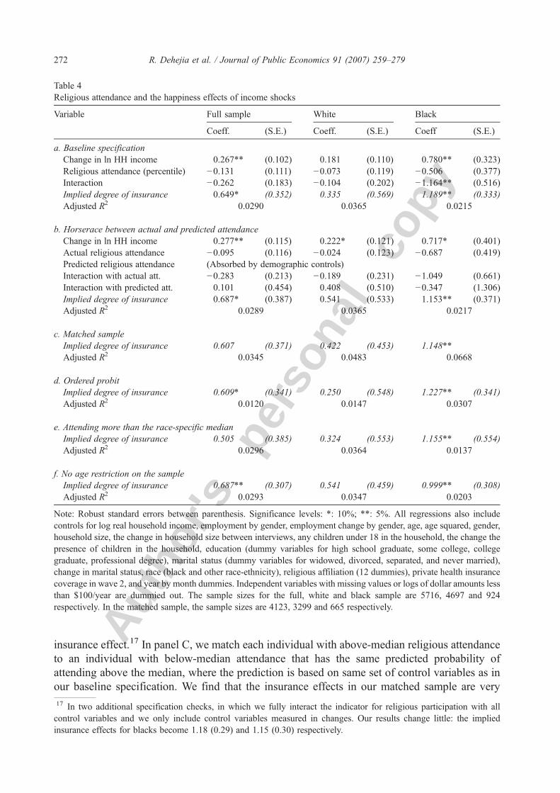
In Table 4, we report the results of our analyses using the NSFH to examine whether religiousparticipation can buffer the happiness consequences of income shocks. The first column of panelA presents our baseline specification for the full sample. As before, a negative coefficient on theinteraction term can be interpreted as religious participation providing an insurance effect. Weestimate the implied degree of insurance as the degree to which going from the 25th percentile ofthe attendance distribution (roughly attending once a year) to the 75th percentile (attendingweekly) reduces the impact of an income shock on happiness.16 The implied degree of insurancefor the full sample is 65% and statistically significant at the 10% level. Thus, roughly speaking,active religious participation buffers about two thirds of the reduction in happiness from anegative income shock.

In columns (2) and (3), we restrict the samples to whites and to blacks and find that our resultsare driven primarily by blacks. For whites, the estimate of the implied degree of insurance is abouta third, but it is not statistically significant. For blacks, however, the implied degree of insurance issignificant at the 1% level and the point estimate suggests roughly full insurance. It is intriguingthat our consumption insurance effects primarily show up for whites while the happinessinsurance effects are strongest for blacks. We discuss and interpret this finding more extensivelyin Section 6.

Panels B and C of Table 4 explore whether the baseline results could be driven by differencesin observable characteristics between active religious participants and less active ones. In panel B,we interact income shocks both with actual and with predicted religious attendance. We find thatactual rather than predicted religious attendance drives our baseline results. Thus actual religiousattendance, rather than observable characteristics correlated with attendance, provides the

15 We report results only for white and black households. Results for the full sample are very similar to those for thewhite sample.16 We measure the implied degree of insurance as the effect of a 50 percentile point increase in attendance forcomparability with Table 2: if we had measured attendance as a dichotomous variable (like membership in Table 2), theaverage attendance among the high attendance group would by definition be 50 percentile points higher than the averageattendance in the low attendance group. Formally, the implied degree of insurance is calculated as −0.5 β3/(β1+0.25 β3),where β1 is the coefficient on the change in income, β3 is the coefficient on the interaction term, and (β1+0.25 β3) is thehappiness sensitivity to income shocks of someone at the 25th percentile of the attendance distribution. In specification E,where attendance is measured by a dummy variable, the implied degree of insurance is given by −β3/β1.


Autho

r's

pers

onal

co

py

Table 3Consumption effects by respondent characteristics

Respondentcharacteristic

Whites Blacks

Δ ln HHincome

Membership Interaction Implied degree ofinsurance

Adj. R2 N Δ ln HHincome

Membership Interaction Implied degree ofinsurance

Adj. R2 N

Coeff. Coeff. Coeff. Coeff. Coeff. Coeff. Coeff. Coeff.

(S.E.) (S.E.) (S.E.) (S.E.) (S.E.) (S.E.) (S.E.) (S.E.)

a. By educational attainmentHigh schoolor less

0.123** 0.005 −0.065 0.524** 0.0330 11588 0.126** −0.022 −0.127* 1.007* 0.1068 1919(0.018) (0.021) (0.043) (0.157) (0.042) (0.044) (0.067) (0.528)

Some collegeor more

0.095** 0.017 −0.027 0.283 0.0271 15602 0.049 0.003 0.037 −0.757 0.1453 1403(0.023) (0.015) (0.038) (0.204) (0.082) (0.058) (0.132) (3.271)

b. By liquid financial assets$2000 or less 0.114** 0.019 −0.047 0.412** 0.0347 13580 0.119** −0.034 −0.103 0.869 0.0946 2612

(0.016) (0.018) (0.039) (0.113) (0.033) (0.031) (0.077) (0.583)More than$2000

0.094** −0.004 −0.032 0.335 0.0306 13610 0.020 0.056 0.058 −2.826 0.2915 710

(0.028) (0.017) (0.048) (0.216) (0.159) (0.093) (0.172) (9.290)

c. By per capita income$15000 or less 0.090** 0.002 −0.062 0.687** 0.0291 13358 0.106** −0.011 −0.064 0.600 0.1002 2322

(0.017) (0.019) (0.032) (0.190) (0.037) (0.039) (0.086) (0.527)More than$15000

0.147** 0.021 −0.030 0.206* 0.0319 13832 0.167 −0.069 −0.124 0.742 0.1757 1000(0.023) (0.015) (0.043) (0.129) (0.134) (0.077) (0.173) (0.630)

Note: Standard errors are calculated accounting for the complex survey design of the CEX and are reported between parenthesis. Significance levels: *: 10%; **: 5%. All regressionsalso include the controls from the baseline regression (Table 2, panel a). Financial assets and per capita income are measured in 2005 constant dollars.

271R.Dehejia

etal.

/Journal

ofPublic

Econom

ics91

(2007)259–279

Autho

r's

pers

onal

co

py

insurance effect.17 In panel C, we match each individual with above-median religious attendanceto an individual with below-median attendance that has the same predicted probability ofattending above the median, where the prediction is based on same set of control variables as inour baseline specification. We find that the insurance effects in our matched sample are very

Table 4Religious attendance and the happiness effects of income shocks

Variable Full sample White Black

Coeff. (S.E.) Coeff. (S.E.) Coeff (S.E.)

a. Baseline specificationChange in ln HH income 0.267** (0.102) 0.181 (0.110) 0.780** (0.323)Religious attendance (percentile) −0.131 (0.111) −0.073 (0.119) −0.506 (0.377)Interaction −0.262 (0.183) −0.104 (0.202) −1.164** (0.516)Implied degree of insurance 0.649* (0.352) 0.335 (0.569) 1.189** (0.333)Adjusted R2 0.0290 0.0365 0.0215

b. Horserace between actual and predicted attendanceChange in ln HH income 0.277** (0.115) 0.222* (0.121) 0.717* (0.401)Actual religious attendance −0.095 (0.116) −0.024 (0.123) −0.687 (0.419)Predicted religious attendance (Absorbed by demographic controls)Interaction with actual att. −0.283 (0.213) −0.189 (0.231) −1.049 (0.661)Interaction with predicted att. 0.101 (0.454) 0.408 (0.510) −0.347 (1.306)Implied degree of insurance 0.687* (0.387) 0.541 (0.533) 1.153** (0.371)Adjusted R2 0.0289 0.0365 0.0217

c. Matched sampleImplied degree of insurance 0.607 (0.371) 0.422 (0.453) 1.148**Adjusted R2 0.0345 0.0483 0.0668

d. Ordered probitImplied degree of insurance 0.609* (0.341) 0.250 (0.548) 1.227** (0.341)Adjusted R2 0.0120 0.0147 0.0307

e. Attending more than the race-specific medianImplied degree of insurance 0.505 (0.385) 0.324 (0.553) 1.155** (0.554)Adjusted R2 0.0296 0.0364 0.0137

f. No age restriction on the sampleImplied degree of insurance 0.687** (0.307) 0.541 (0.459) 0.999** (0.308)Adjusted R2 0.0293 0.0347 0.0203

Note: Robust standard errors between parenthesis. Significance levels: *: 10%; **: 5%. All regressions also includecontrols for log real household income, employment by gender, employment change by gender, age, age squared, gender,household size, the change in household size between interviews, any children under 18 in the household, the change thepresence of children in the household, education (dummy variables for high school graduate, some college, collegegraduate, professional degree), marital status (dummy variables for widowed, divorced, separated, and never married),change in marital status, race (black and other race-ethnicity), religious affiliation (12 dummies), private health insurancecoverage in wave 2, and year by month dummies. Independent variables with missing values or logs of dollar amounts lessthan $100/year are dummied out. The sample sizes for the full, white and black sample are 5716, 4697 and 924respectively. In the matched sample, the sample sizes are 4123, 3299 and 665 respectively.

17 In two additional specification checks, in which we fully interact the indicator for religious participation with allcontrol variables and we only include control variables measured in changes. Our results change little: the impliedinsurance effects for blacks become 1.18 (0.29) and 1.15 (0.30) respectively.


Autho

r's

pers

onal

co

py

similar to those in our baseline sample, though the estimate is no longer marginally statisticallysignificant for the full sample.18

Panels D to F provide robustness checks for the happiness insurance results that are analogousto those provided for the consumption insurance results in Table 2. In particular, we test thesensitivity of our baseline results to: in panel D, running the regressions as an ordered probitrather than OLS; in panel E, measuring religious attendance with an indicator for attending morethan the race-specific mean; and, in panel F, eliminating the age restriction.19 In all cases, theinsurance effect of religious participation is statistically significant for blacks, with pointestimates generally indicating close to full insurance. For whites, the insurance effect is neverstatistically significant, though the point estimates generally indicate a degree of insurance that iseconomically meaningful.20

In Table 5, we examine the insurance effect of religious attendance for subsamples of the data.We split the sample by education, liquid financial assets, per capita income, and the intensity ofreligious belief. In panel A among black individuals, we find a significant insurance effect for lesseducated individuals. For more educated individuals, we find an insurance effect, but one that isnot statistically significant. Among whites, the implied degree of insurance for the less educated islarge but not statistically significant, whereas for the more educated there is an insignificant effectin the opposite direction. In panels B and C, when we split the data by financial assets and by percapita income, which are presumably closely correlated with education and each other, we getvery similar results. Thus, these findings echo the earlier consumption insurance results: theinsurance effects are strongest for less educated, lower wealth and lower income individuals,whether it concerns consumption insurance (Table 3) or happiness insurance (Table 5).

Finally, in panel D,we split our results by intensity of religious beliefs asmeasured by the averageresponse to two statements about the Bible.21 We find that those with the greatest intensity of beliefsexperience the largest insurance effect; among blacks this effect is significant and large inmagnitude,and among whites this effect points in the direction of insurance though it is not significant. Variousmechanisms could give rise to this finding. Religious organizations could treat all participantsequally but those with more intense beliefs might receive more doctrinal solace from attending afterexperiencing a negative income shock. Alternatively, those with more intense beliefs may be more

18 In additional analyses (not reported), conducted to help alleviate the concern that unobservable differences might beresponsible for our results, we first determine whether our estimates of the insurance effect change as we add blocks ofcontrols variables to our models and, second, we determine how sensitive our estimates are to the addition of controls forwealth, homeownership and insurance interacted with changes in income. When adding blocks of controls, we startingwith only demographic controls, add controls for education, third add the level of income as control, and finally add allremaining controls, and find that the implied degree of insurance changes very little: e.g. for blacks it is 1.16 (0.31), 1.17(0.31), 1.16 (0.32), and 1.25 (0.38) respectively. Also when we add additional interactions with income changes, theimplied degree of insurance changes little: e.g. for blacks it is 1.25 (0.40), 1.22 (0.35), 1.13 (0.36), and 1.20 (0.44)respectively as we interact income changes with wealth, homeownership, insurance and all three.19 We also test the sensitivity of our baseline results to measuring income in per capita terms, eliminating the top andbottom coding of income shocks, and measuring religious attendance as times per month rather than as percentiles. Theresults, reported in Dehejia, DeLeire, and Luttmer (2005), are very similar.20 In other robustness checks, which are not shown, we allow for separate insurance effects for increases and decreasesin income; we find that our insurance effect is somewhat stronger for negative income shocks, but the insurance effect isno longer statistically significant when we restrict shocks to only positive or only negative shocks. Hence, we lack powerto distinguish whether the insurance effect is driven by positive or negative shocks.21 Because this question is only relevant for Christians, we drop those reporting a non-Christian religious affiliation fromthe sample in panel D. The statements are “The Bible is God's word and everything happened or will happen exactly as itsays” and “The Bible is the answer to all important human problems” and the response to each statement was recorded ona 5-point scale from “strongly agree” to “strongly disagree”.


Autho

r's

pers

onal

co

py

Table 5Happiness effects by respondent characteristics

Respondentcharacteristic

Whites Blacks

Δ ln HHincome

Membership Interaction Impliedinsurance


Membership Interaction Impliedinsurance

Adj. R2 N



a. By educational attainmentHigh school or less 0.257* −0.175 −0.376 1.154 0.0298 2353 1.079** −0.492 −1.640** 1.225** 0.0203 568

(0.154) (0.176) (0.296) (0.753) (0.410) (0.485) (0.651) (0.362)Some college ormore

0.085 0.042 0.176 −0.680 0.0413 2333 0.339 −0.211 −0.732 2.349 0.0078 355(0.154) (0.164) (0.274) (1.459) (0.556) (0.593) (0.899) (3.234)

b. By liquid financial assets$2000 or less 0.277 −0.145 −0.363 0.977 0.0345 1626 1.101** −0.234 −1.843** 1.439** 0.0136 584

(0.193) (0.238) (0.365) (0.801) (0.436) (0.570) (0.714) (0.397)More than $2000 0.125 −0.047 0.062 −0.221 0.0342 3071 0.300 −0.793 0.068 −0.108 0.0205 340

(0.135) (0.137) (0.243) (0.965) (0.477) (0.502) (0.730) (1.239)

c. By per capita income$15000 or less 0.452* −0.089 −0.364 0.505 0.0412 1588 0.698 −1.107* −1.347* 1.863* 0.0390 503

(0.189) (0.226) (0.344) (0.391) (0.469) (0.565) (0.706) (0.967)More than $15000 0.018 −0.067 0.094 −1.141 0.0374 2989 0.519 0.172 −0.346 0.400 0.0374 354

(0.133) (0.139) (0.248) (4.822) (0.462) (0.556) (0.830) (0.783)

d. By intensity of beliefsBelow median 0.108 0.022 0.240 −0.713 0.0353 2389 0.533 −0.515 −0.774 1.140 0.0215 508

(0.144) (0.186) (0.333) (1.197) (0.390) (0.499) (0.696) (0.755)Above median 0.289 −0.138 −0.319 0.759 0.0453 2029 1.545** 0.004 −2.270** 1.162** 0.0070 387

(0.205) (0.199) (0.318) (0.485) (0.696) (0.725) (0.988) (0.284)

Note: Robust standard errors between parenthesis. Significance levels: *: 10%; **: 5%. All regressions also include the controls from the baseline regression (Table 4, panel a).Financial assets and per capita income are measured in 2005 constant dollars. The median of belief intensity is determined relative to the own sample.

274R.Dehejia

etal.

/Journal

ofPublic

Econom

ics91

(2007)259–279

Autho

r's

pers

onal

co

py

Table 6Other mechanisms of happiness insurance

Mechanism Whites Blacks

Δ ln HHincome

Activity Interaction Impliedinsurance


Activity Interaction Impliedinsurance

Adj. R2 N



a. Social activitiesGetting together socially withfriends/neighbors/relatives

0.210 −0.014 −0.041 0.485 0.0365 4697 0.516* −0.335** −0.234 1.662* 0.0257 924(0.167) (0.052) (0.090) (0.885) (0.289) (0.109) (0.152) (0.877)

Group recreational activity 0.147* −0.005 −0.014 0.206 0.0356 4697 0.204 −0.032 −0.067 0.989 0.0146 924(0.079) (0.027) (0.048) (0.707) (0.189) (0.080) (0.117) (1.805)

Going to a bar 0.089 0.038 0.045 −0.671 0.0363 4697 0.227 −0.037 −0.124 2.423 0.0122 924(0.074) (0.031) (0.051) (0.797) (0.175) (0.095) (0.126) (3.987)

Going to social event at church/synagogue/mosque

0.182** −0.023 −0.051 0.783 0.0366 4697 0.487** 0.141 −0.226* 1.734* 0.0191 924(0.075) (0.039) (0.052) (0.870) (0.238) (0.101) (0.118) (0.926)

b. Activity in organizationsService or political organization 0.202** 0.001 −0.280** 1.384** 0.0371 4697 0.137 0.162 −0.036 0.261 0.0226 924

(0.065) (0.073) (0.138) (0.592) (0.158) (0.201) (0.331) (2.249)Work-related organization 0.120* 0.026 0.044 −0.370 0.0364 4697 0.121 0.529** 0.032 −0.266 0.0283 924

(0.068) (0.072) (0.125) (0.592) (0.168) (0.202) (0.317) (2.882)Leisure groups 0.148* −0.137** −0.031 0.206 0.0368 4697 0.090 0.187 0.113 −1.263 0.0147 924

(0.085) (0.069) (0.120) (0.721) (0.210) (0.200) (0.324) (6.218)Religious organizations 0.191** −0.117 −0.150 0.785 0.0377 4697 0.330 0.198 −0.346 1.048** 0.0145 924

(0.074) (0.085) (0.120) (0.485) (0.236) (0.207) (0.301) (0.492)

Note: Robust standard errors between parenthesis. Significance levels: *: 10%; **: 5%. All regressions also include the controls from the baseline regression (Table 4, panel a). Allthe variables on social activities are measured on a 0–4 scale with 0 corresponding to “never”, 1 to “several times a year”, 2 to “about once a month”, 3 to “about once a week” and 4to “several times per week.” For these variables, the implied degree of insurance is the reduction in the happiness impact of income shocks associated with attendance going from 1to 3. “Getting together socially with friends/neighbors/relatives/colleagues” is measured as the average of four separate questions asked about getting together socially with each ofthese classes of people. “Activity in organizations” equals 1 if the respondent reports to attend at least “several times per year” an event of such an organization. Service and policitalorganizations include service, fraternal, veterans' and political groups. The sample sizes for the white and black sample are 4697 and 924 respectively.

275R.Dehejia

etal.

/Journal

ofPublic

Econom

ics91

(2007)259–279

Autho

r's

pers

onal

co

py

attached to their religious organization (in ways not captured by frequency of attending religiousservice) and the religious organizationmay channel assistance to more attachedmembers. However,in unreported regressions, we found that the intensity of beliefs by itself does not provide happinessinsurance against income shocks. Thus, just believing is not sufficient; one needs to participate in areligious organization to receive happiness insurance.22

It will not be possible for our results to distinguish between the spiritual, social and materialchannels though which religious participation may provide happiness insurance. However, byexamining the insurance effect of other social activities, we can at least determine whether religiousorganizations play a special role in this regard. These results are presented in Table 6. In panel A, weinteract a range of social activitieswith income shocks. For blacks, we find that all social activities goin the direction of providing insurance for happiness against income shocks, but that only gettingtogether socially and going to social events at a church, synagogue or mosque are marginallystatistically significant. For whites, all activities (other than going to a bar) go in the direction ofinsurance, but none are even close to statistical significance. In panel B, we examine the effect ofparticipating in organizations such as political and service groups, leisure groups, work-relatedactivities, and religious organizations. These activities generally do not provide a statistically sig-nificant degree of insurance, except for whites active in service or political organizations and blacksparticipating in church-related events (other than religious service).We conclude that participation inreligious organizations stands out from other measures of social capital in its ability to providehappiness insurance against income shocks.

5.3. Discussion

We find it interesting that the mechanism behind the insurance effects of participation in religiousorganizations appears to differ by race. However, given that our results are based on two differentoutcomes and two different measures of religious participation and because there are no statisticallysignificant differences in the insurance effects between blacks and whites, our results are merelysuggestive that the form of insurance provided by religious organizations differs by race.

Of course, because we use the same measure of participation for blacks and whites within eachdata set, the difference inmeasures alone is unlikely to explain the differences in insurance effects byrace. By contrast, if either attendance or contributions differentiallymeasures participation for blacksand whites, then this difference could explain the differences in insurance effects by race. Forexample, this could arise if all white participants, but not all black participants, of religiousorganizationsmake contributions or if all black participants, but not all white participants of religiousorganizations attend religious services. For this reason, our statistical confidence that the form ofinsurance provided by religious organizations differs by race is limited.

Nonetheless, this finding is consistent with evidence from the sociological literature. Cnaan(2002) finds that percent white membership of a congregation is a significant and positivepredictor of a congregation's financial commitment to giving, even after controlling for theincome and total budget of the congregation. Chaves and Higgins (1992) find that the form inwhich members of religious organizations help each other differs by race. Mutual help in blackchurches is more likely to be in-kind (and thus less likely to be measured by the CEX) whilemutual help in white religious organizations is more likely to be in cash or as a loan (thus showing

22 Another split we consider is by religious denomination (available for the NSFH but not the CEX) and examinewhether religious participation insures against shocks other than income. We do not find any significant results; seeDehejia, DeLeire, and Luttmer (2005).


Autho

r's

pers

onal

co

py

up in expenditures in the CEX). Nelson (1997) notes that the level of trust between differentfamilies belonging to the same church is often remarkably low in poor black communities, andthat this lack of trust may also inhibit short-term loans between members of the churchcommunity.

The relatively small and insignificant happiness insurance effect for whites suggests a stigmaattached to receiving assistance, though we do not have direct evidence for this. Furthermore,moral or doctrinal support for those experiencing difficulties tends to be greater in black churchesthan in white churches, leading to substantial happiness insurance. Nelson (2004), for example,notes that many poor black church members place less emphasis on material sources of happiness;instead, they view those in the middle class as people “who had lost their religious fervor bybecoming too concerned with material goods.” For many African Americans, the church is thecommunity (Carson, 1990). Church services tend to be community-oriented and relatively long(often over 2 h), and there are many well-attended social and community related church events.Thus, relative to whites, African Americans who do not belong to a church may have feweralternative sources of (emotional) support when they fall on hard times. While these explanationsseem plausible, further research on the exact mechanisms bywhich religious organizations provideinsurance remains desirable.

One drawback of the data we use to identify the insurance effects of participation in religiousorganizations is that we cannot identify the mechanism by which this participation buffers againstchanges in income. The amount of cash assistance provided by religious organizations wouldhave to be large to explain these insurance effects. Alternatively, participating in religiousorganizations may provide individuals with sufficient contacts within their community to enablethem to receive aid directly from other individuals when required.

One likely mechanism by which religious organizations may provide consumption insurance isby allowing their members to reduce the amount of their contributions in years following a reductionin their income. By doing so, members would be able to reduce other forms of consumption by less.From our analysis using the NSFH, we observe no decline in attendance in response to a change inincome.23 A decline in contributions in response to a change in income, therefore,would be a formofinsurance since the religious organizations would be continuing to provide services while allowingthe member to make fewer (or no) contributions.

Unfortunately, we are unable to identify the extent of this possible insurance mechanism sincewe only observe annual religious contributions in the fourth interview in the CEX data.

6. Conclusion

We find that religious participation partially insures consumption and happiness against incomeshocks. This finding has important implications for the public provision of social insurance. Socialinsurance is less valuable for those who are already partly insured through their religiousorganization, implying that the optimal level of social insurance is inversely related to the religiousparticipation of the population.24 Conversely, social insurance can crowd out insurance provided byreligious organizations. Thus, even where church and state are officially separated, governmentsproviding less social insurance will indirectly stimulate the demand for insurance from religiousorganizations and thus mostly likely strengthen the influence of religious organizations.

23 These results are reported in Dehejia, DeLeire, and Luttmer (2005).24 Of course, insurance provided by religious organizations may crowd out other forms of private insurance, such as thatprovided by extended families.


Autho

r's

pers

onal

co

py

References

Altonji, Joseph G., Hayashi, Fumio, Kotlikoff, Laurence J., 1997. Parental altruism and inter vivos transfers: theory andevidence. Journal of Political Economy 105 (6), 1121–1166.

Altonji, Joseph G., Elder, Todd E., Taber, Christopher, 2005. Selection on observable and unobservable variables:assessing the effectiveness of Catholic schools. Journal of Political Economy 113 (1), 151–184.

Attanasio, Orazio, Davis, Steven J., 1996. Relative wage movements and the distribution of consumption. Journal ofPolitical Economy 104 (6), 1227–1262.

Azzi, Corry, Ehrenberg, Ronald G., 1975. Household allocation of time and church attendance. Journal of PoliticalEconomy 83 (1), 27–56.

Barro, Robert J., McCleary, Rachel, 2003. Religion and economic growth. National Bureau of Economic ResearchWorking Paper, vol. 9682.

Berman, Eli, 2000. Sect, subsidy, and sacrifice: an economist's view of ultra-orthodox Jews. Quarterly Journal ofEconomics 115 (3), 905–953.

Biddle, Jeff E., 1992. Religious organizations. In: Clotfelter, Charles T. (Ed.), Who Benefits From the Non-Profit Sector?University of Chicago, Chicago.

Blanchflower, David G., Oswald, Andrew J., 2004. Well-being over time in Britain and the USA. Journal of PublicEconomics 88 (7–8), 1359–1386.

Carson, Emmett, 1990. Patterns of giving in Black churches. In: Wuthnow, Robert, Hodgkinson, Virginia (Eds.), Faith andPhilanthropy in America: Exploring the Role of Religion in America's Voluntary Sector. Jossey-Bass Publishers, SanFrancisco, pp. 232–252.

Chaves, Mark, Higgins, Lynn, 1992. Comparing the community involvement of Black and White congregations. Journalfor the Scientific Study of Religion 31 (4), 425–440.

Chen, Daniel, 2004. Club goods and group identity: evidence from the Islamic resurgence during the Indonesian financialcrisis. University of Chicago. manuscript.

Clark, Andrew, Lelkes, Orsolya, 2005. Deliver Us From Evil: Religion as Insurance. PSE, Paris. manuscript.Cnaan, Ram, 2002. The Invisible Caring Hand: American Congregations and the Provision of Welfare. New York

University Press, New York.Cochrane, John A., 1991. A simple test of consumption insurance. Journal of Political Economy 99 (5), 957–976.Cox, Donald, 1987. Motives for private income transfers. Journal of Political Economy 95 (3), 508–546.Cullen, Julie Berry, Gruber, Jonathan, 2000. Does unemployment insurance crowd out spousal labor supply? Journal of

Labor Economics 18 (3), 546–572.Deaton, Angus, 1992a. Understanding Consumption. Clarendon Press, Oxford.Deaton, Angus, 1992b. Household saving in LDCs: credit markets, insurance, and welfare. Scandinavian Journal of

Economics 94 (2), 253–273.Dehejia, Rajeev, DeLeire, Thomas, Luttmer, Erzo F.P., 2005. Insuring consumption and happiness through religious

organizations. National Bureau of Economic Research Working Paper, vol. 11576.Diener, Ed, Biswas-Diener, Robert, 2002. Will money increase subjective well-being? Social Indicators Research 57, 119–169.Diener, Ed, Suh, Eunkook M., Lucas, Richard E., Smith, Heidi L., 1999. Subjective well-being: three decades of progress.

Psychological Bulletin 125 (2), 276–303.Di Tella, Rafael, Haisken-De New, John, MacCulloch, Robert, 2005. Adaptation to Income and Status in an Individual

Panel. Harvard University. Manuscript.Ellison, Christopher G., 1991. Religious involvement and subjective well-being. Journal of Health and Social Behavior 32

(1), 80–99.Foster, Andrew, Rosenzweig, Mark, 2001. Imperfect commitment, altruism, and the family: evidence from transfer

behavior in low-income rural areas. Review of Economics and Statistics 83 (3), 389–407.Freeman, Richard B., 1986. Who escapes? The relation of churchgoing and other background factors to the socioeconomic

performance of Black male youths from inner-city tracts. In: Freeman, Richard B., Holzer, Harry J. (Eds.), The BlackYouth Employment Crisis. University of Chicago Press, Chicago, pp. 353–376.

Frey, Bruno S., Stutzer, Alois, 2002. What can economists learn from happiness research? Journal of Economic Literature40 (2), 402–435.

Friedman, Milton, 1957. A Theory of the Consumption Function. Princeton University Press, Princeton.Gardner, Jonathan, Oswald, Andrew J., 2005. Money and Mental Health: a Study of Medium-Sized Lottery Wins.

University of Warwick. Manuscript.Genicot, Garance, Ray, Debraj, 2003. Group Formation in Risk-Sharing Agreements. Review of Economic Studies 70 (1),

87–113.


Autho

r's

pers

onal

co

py

Gertler, Paul, Gruber, Jonathan, 2002. Insuring consumption against illness. American Economic Review 92 (1), 51–70.Guiso, Luigi, Sapienza, Paola, Zingales, Luigi, 2003. People's opium? Religion and economic attitudes. Journal of

Monetary Economics 50, 225–282.Gruber, Jonathan, 2004. Pay or pray? The impact of charitable subsidies on religious attendance. Journal of Public

Economics 88 (12), 2635–2655.Gruber, Jonathan, 2005. Religious market structure, religious participation, and outcomes: is religion good for you?

Advances in Economic Analysis and Policy 5 (1) (Article 5. Available at http://www.bepress.com/bejeap/advances/vol5/iss1/art5).

Gruber, Jonathan, Hungerman, Daniel M., 2005. Faith-based charity and crowd out during the Great Depression. NationalBureau of Economic Research Working Paper, vol. 11332.

Gruber, Jonathan, Mullainathan, Sendhil, 2005. Do cigarette taxes make smokers happier? Advances in EconomicAnalysis and Policy 5 (1) (Article 4. Available at http://www.bepress.com/bejeap/advances/vol5/iss1/art4).

Hungerman, Daniel M., 2005. Are church and state substitutes? Evidence from the 1996Welfare Reform. Journal of PublicEconomics 89 (11–12), 2245–2267.

Iannaccone, Laurence R., 1990. Religious participation: a human capital approach. Journal for the Scientific Study ofReligion 29 (3), 297–314.

Iannaccone, Laurence R., 1992. Sacrifice and stigma: reducing free-riding in cults, communes, and other collectives.Journal of Political Economy 100 (2), 271–291.

Iannaccone, Laurence R., 1998. Introduction to the economics of religion. Journal of Economic Literature 36 (3),1465–1495.

Leland, Hayne E., 1968. Saving and uncertainty. Quarterly Journal of Economics 82 (3), 465–473.MacCulloch, Robert, Pezzini, Silvia, 2004. The Role of Freedom, Growth and Religion in the Taste for Revolution.

Imperial College, London. Manuscript.Mace, Barbara J., 1991. Full insurance in the presence of aggregate uncertainty. Journal of Political Economy 99 (5), 928–956.McCullough, Michael E., Hoyt, William T., Larson, David B., Koenig, Harold G., Thoresen, Carl, 2000. Religious

involvement and mortality: a meta-analytic review. Health Psychology 19 (3), 211–222.Nelson, Julie A., 1994. On testing for full insurance using Consumer Expenditure Survey data. Journal of Political

Economy 102 (2), 384–394.Nelson, Timothy J., 1997. The church and the street: race and poverty in an inner-city congregation. In: Becker, Penny

Edgell, Eiesland, Nancy (Eds.), Contemporary American Religion: an Ethnographic Reader. Alta Mira Press.Nelson, Timothy J., 2004. Every Time I Feel the Spirit: Religious Ritual and Experience in an African American Church.

New York University Press, New York.Pargament, Kenneth I., 2002. The bitter and the sweet: an evaluation of the costs and benefits of religiousness.

Psychological Inquiry 13 (3), 168–181.Putman, Robert D., 2000. Bowling Alone: the Collapse and Revival of American Community. Simon & Schuster, New

York.Stasavage, David, Scheve, Ken, 2005. Religion and Preferences for Social Insurance. London School of Economics.

Manuscript.Stasavage, David, Scheve, K., 2006. The Political Economy of Religion and Social Insurance in the United States, 1910–

1939. London School of Economics. Manuscript.Strawbridge, William J., Shema, Sarah J., Cohen, Richard D., Roberts, Robert E., Kaplan, George A., 1998. Religiosity

buffers effects of some stressors on depression but exacerbates others. Journals of Gerontology 53B (3), 118–126.Smith, Timothy B., McCullough, Michael E., Poll, Justin, 2003. Religiousness and depression: evidence for a main effect

and the moderating influence of stressful life events. Psychological Bulletin 129 (4), 614–636.Sweet, James A., Bumpass, Larry L., 1996. The National Survey of Families and Households—Waves 1 and 2: Data

Description and Documentation. Center for Demography and Ecology, University of Wisconsin-Madison. http://www.ssc.wisc.edu/nsfh/home.htm.

Sweet, James A., Bumpass, Larry L., Call, Vaughn, 1988. The Design and Content of The National Survey of Families andHouseholds. NSFH Working Paper, vol. 1. Center for Demography and Ecology, University of Wisconsin-Madison.

Townsend, Robert M., 1994. Risk and insurance in village India. Econometrica 62 (3), 539–591.


insuring consumption and happiness through religious...

Documents