integer programming based heterogeneous cpu-gpu cluster schedulers...
TRANSCRIPT

Integer Programming Based Heterogeneous CPU-GPU ClusterSchedulers for SLURM Resource Manager
Seren Sonera, Can Ozturana,∗
aDepartment of Computer Engineering, Bogazici University, Istanbul, Turkey
Abstract
We present two integer programming based heterogeneous CPU-GPU cluster schedulers, called IPSCHED
and AUCSCHED, for the widely used SLURM resource manager. Our scheduler algorithms take windows
of jobs and solve allocation problems in which free CPU cores and GPU cards are allocated collectively to
jobs so as to maximize some objective functions. Our AUCSCHED scheduler employs an auction based
approach in which bids for contiguous blocks of resources are generated for each job. We perform realistic
SLURM emulation tests using the Effective System Performance (ESP) and our own synthetic workloads.
Even though it is difficult to generalize, the tests roughly show that out of the three scheduling plugins,
AUCSCHED achieves better utilization, spread and packing, IPSCHED achieves better waiting time and
SLURM Backfill achieves better fragmentation performances when compared with each other. The SLURM
scheduler plug-ins that implement our algorithm are available at http://code.google.com/p/slurm-ipsched/.
Keywords:
job scheduling, slurm, integer programming,
1. Introduction
SLURM [1] is an open-source resource management software distributed under the GPL license. It
was designed with simplicity, portability and scalability in mind. It has a plug-in mechanism that can be
used by developers to easily extend SLURM functionality by writing their own plug-ins. Older versions of
SLURM had a simple first-come-first-served (FCFS) scheduler, but the recently introduced new version has
advanced features such as backfilling, fair share, preemption, multi-priority, advanced reservation. Some
supercomputer centers use SLURM coupled with other schedulers such as MOAB [2], Maui [3] and LSF [4].
SLURM has been receiving a lot of attention from the supercomputer centers lately. It is used on many
TOP500 supercomputers. It is estimated by SLURM developers that as many as 30% of the supercomputers
in the November 2012 TOP500 list are using SLURM [5]. In particular, it is stated that one third of the 15
∗Corresponding author
Email addresses: [email protected] (Seren Soner), [email protected] (Can Ozturan )
Preprint submitted to Journal of Computer and System Sciences October 4, 2013

most powerful systems in this list use SLURM. These are: No. 2 Sequoia at Lawrence Livermore National
Laboratory, No. 7 Stampede at Texas Advanced Computing Center; No. 8 Tianhe-1A at the National
Supercomputing Center in China, No. 11 Curie at the French Alternative Energies and Atomic Energy
Commission (CEA) and No. 15 Helios at Japan’s International Fusion Energy Research Center.
Recently, heterogeneous clusters and supercomputers that employ both ordinary CPUs and GPUs have
started to appear. Currently, such systems typically have 8 or 12 CPU cores and 1-4 GPU per node. Jobs
that utilize only CPU cores or both CPU cores and GPUs can be submitted to the system. Job schedulers
like SLURM take one job at a time from the front of the job queue; go through the list of nodes and best-fit
the job’s resource requirements to the nodes that have available resources. In such systems, GPU resources
can be wasted if the job scheduler assigns jobs that utilize only CPU cores to the nodes that have both free
CPU cores and GPUs. Table 1 illustrates this problem on a system with 1024 nodes with each node having
8 cores and 2 GPUs. The example submits three sleep jobs each of which lasts for 1000 seconds. Suppose
jobs J1, J2, J3 appear in the queue in this order (with J1 at the front of the queue, J2 second and J3 third).
Note that SLURM will grant jobs J1 and J2 with the requested resources immediately as follows:
• J1 will be best-fit on 512 nodes, hence allowing no other jobs to use the GPUs on these nodes.
• J2 will be allocated 512 nodes using 4 cores and 2 GPUs on each node.
This allocation, however, will cause J3 to wait 1000 seconds until J1 and J2 are finished. On the other
hand, if we take all the jobs, J1, J2 and J3, collectively and solve an assignment problem, it is possible to
allocate the requested resources to all the jobs and finish execution of all of jobs in 1000 seconds rather than
in 2000 seconds. This can be done by assigning 512 nodes with 4 cores and 2 GPUs to each of jobs J2 and
J3 and 1024 nodes with 4 cores to J1.
Table 1: Example illustrating advantage of solving collective allocation problem
Job Resources Requested Slurm Command
J1 4096 cores srun -n 4096 sleep 1000
J22048 cores on 512 srun -N 512 --gres=gpu:2
nodes with 2 GPUs per node -n 2048 sleep 1000
J32048 cores on 512 srun -N 512 --gres=gpu:2
nodes with 2 GPUs per node -n 2048 sleep 1000
In this paper, we are motivated by the scenario exemplified by Table 1 to develop two scheduling algo-
rithms and corresponding plug-ins for SLURM that collectively take a number of jobs and solve assignment
problems among the jobs and the available resources. The assignment problems that are solved at each step
of scheduling are formulated and solved as integer programming (IP) problems. Our first algorithm is based
2
on a knapsack-like formulation [6]. It also attempts to optimize the number of nodes over which a job’s
allocated resources are spread. It, however, does not pay attention to whether the nodes allocated to a job
are allocated within close vicinity of each other. This can be important especially if a job involves multiple
processes that need to do communication which is usually the case for parallel jobs running on a cluster.
To address this issue, we develop a second algorithm that also pays attention to the contiguity of nodes on
which a job is allocated. Especially, if a hierarchy of communication switches are used to connect the nodes
and if allocations are done on neighboring nodes, then a smaller number of switches need to be involved in
the communication. The second algorithm looks into this problem within the context of linear mapping of
jobs to one-dimensional array of nodes. This is the default mode of resource selection in SLURM. SLURM
documentation [7] states the following about this mode: “SLURM’s native mode of resource selection is to
consider the nodes as a one-dimensional array. Jobs are allocated resources on a best-fit basis. For larger
jobs, this minimizes the number of sets of consecutive nodes allocated to the job.”
In the rest of the paper, we first present related works on job schedulers in Section 2. Then, we present the
details our first IP based scheduler algorithm and its corresponding plug-in, called IPSCHED, in Section 3.
Our second algorithm, called AUCSCHED, performs contiguity aware job placement and is presented in
Section 4. To test the performance of our plug-ins, we preferred to carry out realistic direct SLURM
emulation tests rather than use a simulator. The details of the benchmark tests and the results obtained are
given in Sections 5 and 6 respectively. We conclude the paper with a discussion in Section 7. The SLURM
scheduler plug-ins that implement our algorithms are available at http://code.google.com/p/slurm-ipsched/.
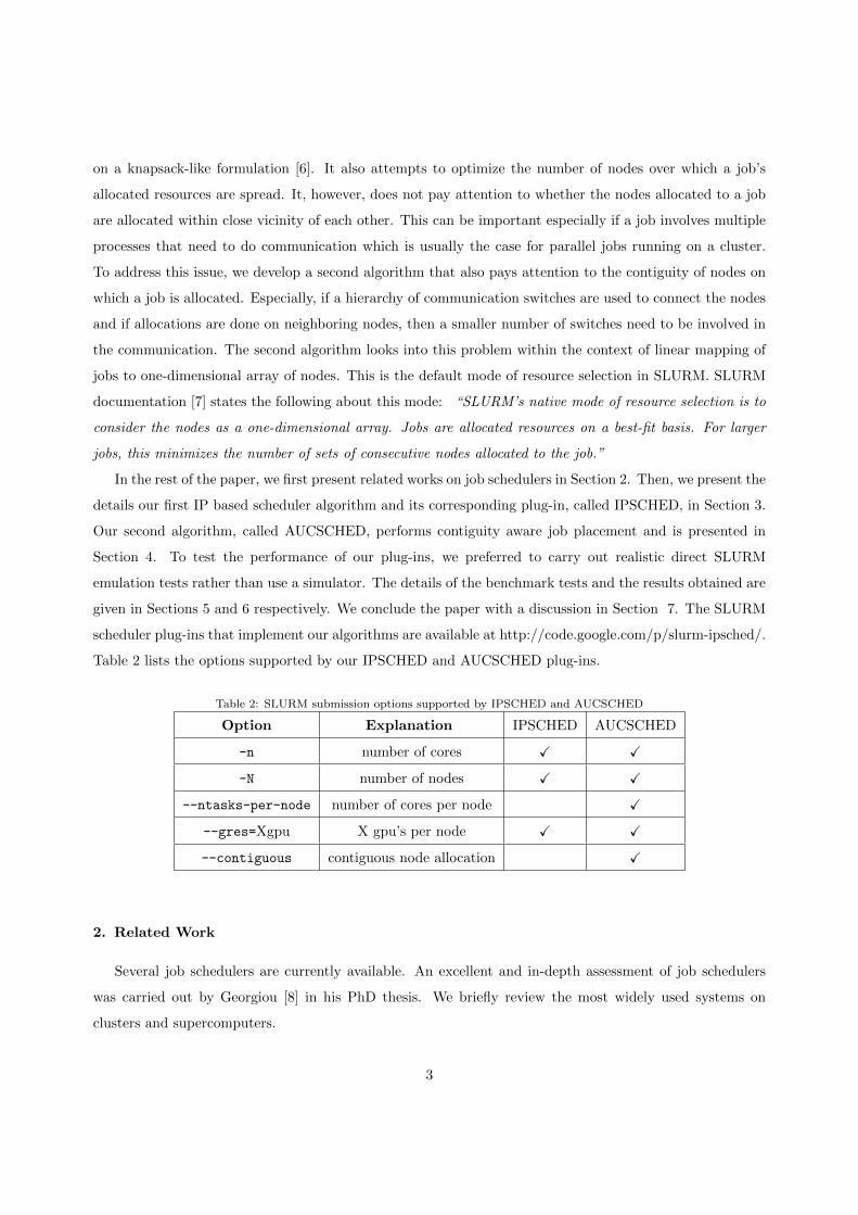
Table 2 lists the options supported by our IPSCHED and AUCSCHED plug-ins.
Table 2: SLURM submission options supported by IPSCHED and AUCSCHED
Option Explanation IPSCHED AUCSCHED
-n number of cores X X
-N number of nodes X X
--ntasks-per-node number of cores per node X
--gres=Xgpu X gpu’s per node X X
--contiguous contiguous node allocation X
2. Related Work
Several job schedulers are currently available. An excellent and in-depth assessment of job schedulers
was carried out by Georgiou [8] in his PhD thesis. We briefly review the most widely used systems on
clusters and supercomputers.
3

PBSpro [9] is a commercial scheduler which descended from the PBS system originally developed in
NASA. In addition to the professional PBSpro, an unsupported original open source version called OpenPBS
is also available. PBSPro has the usual scheduler features: FCFS, backfilling, fair share, preemption, multi-
priority, external scheduler support, advanced reservation support and application licenses. Recently, GPU
scheduling support has been introduced by providing two approaches: (i) simple approach in which only
one GPU job at a time is run on any given node exclusively and (ii) advanced distributed approach which
is needed when sharing of the nodes by multiple jobs at the same time is required or if individual access to
GPUs by device number is required.
MOAB [2] is a commercial job scheduler that originated from the PBS system. It supports the usual
FCFS, backfilling, fair share, preemption, multi-priority, advanced reservation and application licenses.
MOAB is just a scheduler and hence it needs to be coupled with a resource manager system.
TORQUE [10] is a resource management that is the open-source version of PBSPro. Similarly, MAUI
[3] is a scheduler that is open-source version of the MOAB. MAUI supports FCFS, backfilling, fair-share,
preemption, multi-priority, advanced reservation and application licenses. TORQUE also has some GPU
support. Jobs can specify their request for the GPUs but it is left up to the job’s owner to make sure that
the job executes properly on the GPU.
LSF [4] is a commercial scheduler which descended from the UTOPIA system. Like the other schedulers,
it supports FCFS, backfilling, fair-share, preemption, multi-priority, advanced reservation and application
licenses. Newer features include live cluster reconfiguration, SLA-driven scheduling, delegation of adminis-
trative rights and GPU-aware scheduling. LSF can also be fed with thermal data from inside of the servers so
that it can try to balance workloads across server nodes so as to minimize hot areas in clusters. LoadLeveler
[11] is a commercial product from IBM. It was initially based on the open-source CONDOR system [12].
It supports FCFS, backfilling, fair-share, preemption, multi-priority, advanced reservation and application
licenses. It has a special scheduling algorithm for the Blue Gene machine which extends LoadLeveler’s
reliable performance.
OAR [13] is a recently developed open source resource management system for high performance com-
puting. It is the default resource manager for the Grid500 which is a big real-scale experimental platform
where computer scientists can run large distributed computing experiments under real life conditions. OAR
has been mostly implemented in Perl. In addition to the above systems, Condor [12] and Oracle Grid Engine
[14] (formerly known as Sun Grid Engine) systems are also widely used, especially in grid environments.
Since heterogeneous CPU-GPU systems have appeared very recently, we do not expect that the afore-
mentioned commercial or open source job schedulers have done much for optimizing scheduling of such
systems. For example, SLURM has introduced support for GPUs but its scheduling algorithms were not
optimized for GPUs as we illustrated with the example in Table 1. In fact, in SLURM, if the number of
nodes (with -N option) is not specified and just the number of cores (with -n) are given together with the
4
number of GPUs per node (with –gres=gpu:), then this can actually lead to different total number GPUs to
be allocated in different runs of the same job (since the number of GPUs allocated depends on the number
of nodes over which the requested cores are allocated).
In this paper, we employ IP techniques in order to get the assignment of jobs to the resources. IP
techniques have been used for scheduling before. For example, [15] used IP techniques for devising a
dynamic voltage frequency scaling (DVFS) aware scheduler. [16] solved a relaxed IP problem to implement
collective match-making heuristics for scheduling jobs in grids.
The second contiguity aware scheduling algorithm, AUCSCHED, developed in this paper is auction
based. The auction mechanism we implement for SLURM has some similarities to the previous work we
did on multi-unit nondiscriminatory combinatorial auctions [17]. Work on contiguous node allocation of
jobs within the context of first-come-first served with backfilling policy on k-ary n-tree networks have been
carried out by [18]. In [18], non-contiguous, contiguous and a relaxed version of contiguous, called, quasi-
contiguous allocations of jobs were studied by performing simulations. It was reported that contiguous
allocations resulted in severe scheduling inefficiency due to increased system fragmentation. Their proposed
quasi-contiguous approach reduced this adverse effect. Their simulations were carried out by using the
INSEE simulator [19]. Also, they did not address CPU-GPU scheduling and used workloads from the
Parallel Workload Archive [20].
In this paper, we contribute two different IP formulations for node based CPU-GPU systems and imple-
ment two different SLURM plug-ins for it. We are not aware of any other IP based scheduling plug-in that
has been developed for SLURM.
3. IPSCHED Scheduler
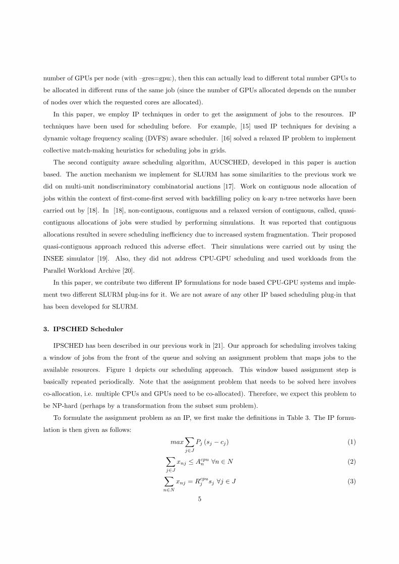
IPSCHED has been described in our previous work in [21]. Our approach for scheduling involves taking
a window of jobs from the front of the queue and solving an assignment problem that maps jobs to the
available resources. Figure 1 depicts our scheduling approach. This window based assignment step is
basically repeated periodically. Note that the assignment problem that needs to be solved here involves
co-allocation, i.e. multiple CPUs and GPUs need to be co-allocated). Therefore, we expect this problem to
be NP-hard (perhaps by a transformation from the subset sum problem).
To formulate the assignment problem as an IP, we first make the definitions in Table 3. The IP formu-
lation is then given as follows:
max∑j∈J
Pj (sj − cj) (1)
∑j∈J
xnj ≤ Acpun ∀n ∈ N (2)
∑n∈N
xnj = Rcpuj sj ∀j ∈ J (3)
5
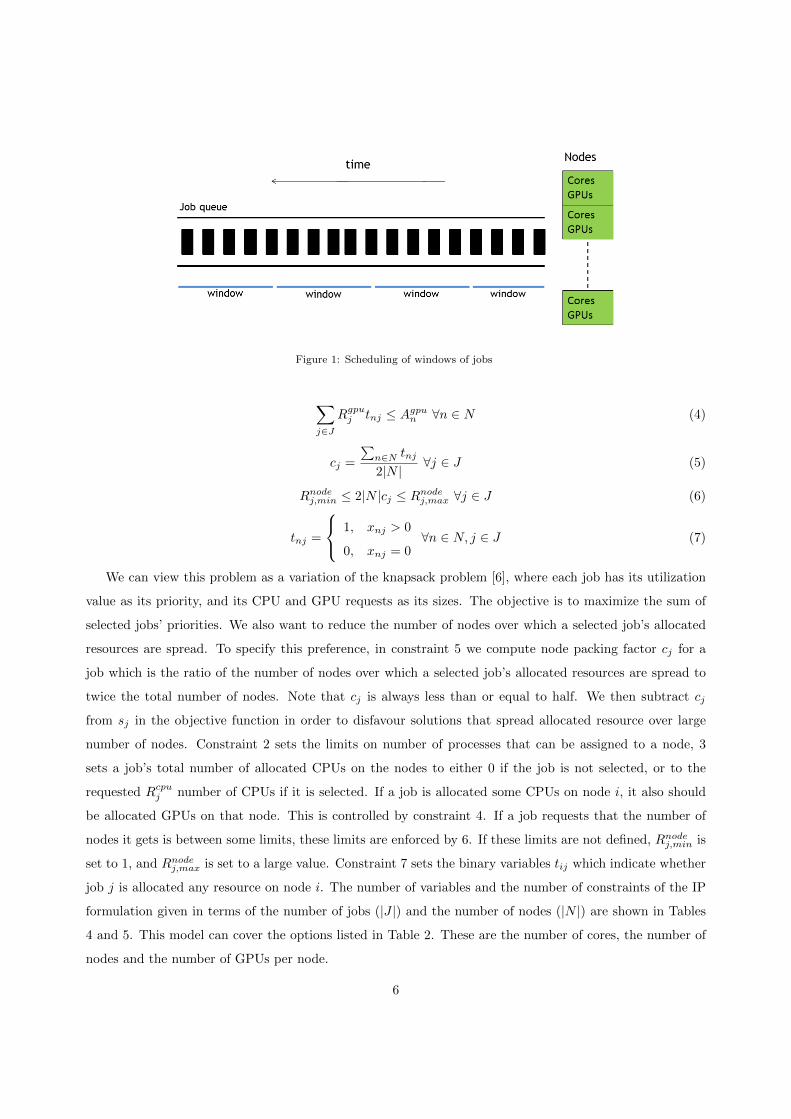
Figure 1: Scheduling of windows of jobs
∑j∈J
Rgpuj tnj ≤ Agpu
n ∀n ∈ N (4)
cj =
∑n∈N tnj
2|N |∀j ∈ J (5)
Rnodej,min ≤ 2|N |cj ≤ Rnode
j,max ∀j ∈ J (6)
tnj =
1, xnj > 0
0, xnj = 0∀n ∈ N, j ∈ J (7)
We can view this problem as a variation of the knapsack problem [6], where each job has its utilization
value as its priority, and its CPU and GPU requests as its sizes. The objective is to maximize the sum of
selected jobs’ priorities. We also want to reduce the number of nodes over which a selected job’s allocated
resources are spread. To specify this preference, in constraint 5 we compute node packing factor cj for a
job which is the ratio of the number of nodes over which a selected job’s allocated resources are spread to
twice the total number of nodes. Note that cj is always less than or equal to half. We then subtract cj
from sj in the objective function in order to disfavour solutions that spread allocated resource over large
number of nodes. Constraint 2 sets the limits on number of processes that can be assigned to a node, 3
sets a job’s total number of allocated CPUs on the nodes to either 0 if the job is not selected, or to the
requested Rcpuj number of CPUs if it is selected. If a job is allocated some CPUs on node i, it also should
be allocated GPUs on that node. This is controlled by constraint 4. If a job requests that the number of
nodes it gets is between some limits, these limits are enforced by 6. If these limits are not defined, Rnodej,min is
set to 1, and Rnodej,max is set to a large value. Constraint 7 sets the binary variables tij which indicate whether
job j is allocated any resource on node i. The number of variables and the number of constraints of the IP
formulation given in terms of the number of jobs (|J |) and the number of nodes (|N |) are shown in Tables
4 and 5. This model can cover the options listed in Table 2. These are the number of cores, the number of
nodes and the number of GPUs per node.
6

Table 3: List of main symbols, their meanings, and definitions for IPSCHED
Symbol Meaning
J Set of jobs that are in the window: J = {j1, . . . , j|J|}
Pj Priority of job j
N Set of nodes : N = {n1, . . . , n|N |}
Acpun Number of available CPU cores on node n
Agpun Number of available GPUs on node n
Rcpuj Number of cores requested by job j
Rgpuj Number of GPUs per node requested by job j
Rnodej,min Minimum number of nodes requested by job j
Rnodej,max Maximum number of nodes requested by job j
sj Binary variable indicating whether job j is allocated or not,
cj node packing variable for a job j,
xnj no. of cores allocated to job j at node n,
tnj binary variable showing whether job j is allocated any resource
on node n.
3.1. Implementation of IPSCHED Plug-in
SLURM employs a central controller daemon (slurmctld) that runs on a central or a management node
and daemons (slurmd) that run on each compute node. Each slurmd daemon interacts with the controller
daemon, and passes information about the job currently running on that node and the node’s status [1].
SLURM has been designed as a light-weight system. In SLURM, almost everything is handled by plug-
ins. SLURM provides several plug-ins such as scheduler, resource selection, topology and priority plug-ins.
The plug-in which we focus on is the scheduler plug-in which works on the controller daemon. SLURM’s
backfill scheduler creates a priority queue, and collects the resource requirements of each job in the queue.
The scheduler tries to start a job by taking into consideration the reservations made by other higher priority
jobs also. If it can fit a job on the nodes with available resources, the job is started; otherwise, it is scheduled
to be started later [7].
The selection of the specific resources is handled by a plug-in called resource selection. SLURM also pro-
vides a resource selection plug-ins called linear that allocates whole nodes to jobs and consumable resources
that allocates individual processors and/or memory to jobs [7]. In this work, a plug-in called IPCONSRES
was designed, which is a variation of SLURM’s own cons res plug-in. IPCONSRES allows our IP based
scheduler plug-in (which we named IPSCHED) to make decisions about the node layouts of the selected
jobs.
7

Table 4: Number of variables in the IP formulation
Variable name Number of variables
sj |J |
cj |J |
xij |J | × |N |
tij |J | × |N |
Total 2|J | × (1 + |N |)
Table 5: Number of constraints in the IP formulation
Constraint Number of constraints
2 |N |
3 |J |
4 |N |
5 |J |
6 2|N |
7 2|J ||N |
Total 2× (|J |+ 2|N |+ |J ||N |)
The priorities of the jobs are calculated by SLURM. Our plug-in does not change these values, but only
collects them while when an assignment problem is solved. In this work, two types of test runs were made.
In the first type of runs, priority type was selected as basic in SLURM. This corresponds to a first-come-first-
served scheduling. SLURM takes the first submitted job’s priority to be a large number, and every arriving
job’s priority will be one less than that of the previously arrived job. In the second type of runs, SLURM’s
multifactor priority plug-in was used. This plug-in allows the job priorities to increase with increasing job
size and aging. Multifactor priority is calculated using parameters such as the age, the job size, fair-share
partition and QOS. The settings of priority factors used in this work are explained in Section 6, namely the
Results section.
In SLURM, GPUs are handled as generic resources. Each node has a specified number of GPUs (and
other generic resources if defined) dedicated to that node. When a user submits a job that uses GPUs,
he has to state the number of GPUs per node that he requests. The GPU request can be 0 if the job
is running only on CPU. The IPSCHED plug-in has been designed in such a way that only one small
change needs to be made to the common files used by SLURM. This change which is located in SLURM’s
common/job scheduler.c file disables the FIFO scheduler of SLURM; thus allowing each job to be scheduled
by our IPSCHED plug-in. Even if the queue is empty and the nodes are idle, a submitted job will wait a
certain number of seconds (named as SCHED INTERVAL) and run when it is scheduled by our IPSCHED
8

Algorithm 1 IPSCHED scheduling steps
1: Generate priority ordered job window of size up to MAX JOB COUNT
2: From each job j in the window, collect the following into job list array
3: a. priority Pj
4: b. CPU request Rcpuj
5: c. GPU request Rgpuj
6: From each node n in the system, collect the following into node info array
7: a. number of empty CPU’s Acpun
8: b. number of empty GPU’s Agpun
9: Form the IP problem
10: Solve the IP problem and get sj and xnj values
11: For jobs with sj = 1, set jobs process layout matrix and start the job by
12: a. For each node n, assign processors on that node according to xnj
13: b. Start the job, no more node selection algorithm is necessary.
plug-in. IPSCHED plug-in runs every SCHED INTERVAL seconds. By default this value is 3 and can
be changed in the SLURM configuration file. IPSCHED solves the IP problem we defined in Section 3 to
decide which jobs are to be allocated resources.
The workings of our plug-in are explained in the pseudo-code given in Algorithm 1. The plug-in first gets
a window of the priority ordered jobs. The number of jobs in the window is limited by MAX JOB COUNT
variable (by default this is set to 200 but can be changed using SLURM configuration file). The plug-in also
collects the job priority, number of CPUs and GPUs requested and store these in the PJ , Rcpuj and Rgpu
j
arrays. Afterwards, it obtains the “empty CPU” and “empty GPU” information from all the nodes and
stores these values in Acpun and Agpu
n arrays. The Acpun , Agpu
n , PJ and Rcpuj values are then used to create
the integer programming problem, which is solved using CPLEX [22].
The SCHED INTERVAL is also used to set a time limit during the solution of the IP problem. If the
time limit is exceeded, in that scheduling interval, none of the jobs are started, and the number of jobs in
the window is halved for the next scheduling interval. In step 6, a layout matrix which has nodes as columns
and selected jobs as rows is used to show mapping of jobs to the nodes. This matrix is used to assign and
start the job on its allocated nodes.
Note that IPSCHED can handle a job’s minimum/maximum and processor/node requests but it assumes
that the jobs do not have explicit node requests. Such job definitions may break up the system, since the
selection of jobs is made based only on the availability of resources on the nodes.
Finally, we also note that our IPSCHED plug-in has been developed and tested on version 2.3.3 of
SLURM, which was the latest stable version during the time of development.
9

4. AUCSCHED: Contiguity-Aware Scheduler
If a job is allocated some resources, then depending on what resources it has been assigned, the job itself
may perform tuning to achieve better performance on these resources, for example, by using topologically
aware communication. A complementary tuning can also be performed by the scheduler of a resource
manager by helping a job to achieve better run-time performance by placing it on resources that will lead to
faster execution. Such may be the case, for example, if a communication intensive job is allocated nodes that
are in close vicinity to each other. Since a scheduler has access to information about available resources and
is the authority that makes allocation decisions, it can enumerate and consider alternative candidate resource
allocations to each job. This model considers this complementary approach that aims to tune mappings of
jobs at the scheduling level. AUCSCHED attempts to allocate contiguous blocks on one-dimensional array
of nodes. Table 2 lists the SLURM options that our plug-in AUCSCHED supports. The number of cores
per node and the option that states whether the allocation is explicitly requested to be contiguous can be
given as options to AUCSCHED additional to the options supported by IPSCHED.
Our proposed methodology is similar to that of the IPSCHED scheduler discussed earlier. Our algorithm
takes a window of jobs from the front of the job queue, generates multiple bids for available resources for
each job, and solves an assignment problem that maximizes an objective function involving priorities of
jobs. To achieve a topologically aware mapping of jobs to processors, the bids generated include requests
for contiguous allocations. Given the list of additional symbols and their meanings in Table 6, the IP
formulation of AUCSCHED is as follows:
Maximize∑j∈J
∑c∈Bj
(Pj + α · Fjc) · bjc (8)
subject to constraints :
∑c∈Bj
bjc ≤ 1 for each j ∈ J (9)
∑n∈Nc
ujn = bjc ·Rnodejc
for each (j, c) ∈ J × C s.t. c ∈ Bj (10)
∑n∈Nc
∑c∈Bj
ujn + rjn =∑c∈Bj
bjc ·Rcpujc for each j ∈ J (11)
∑j∈J
ujn + rjn ≤ Acpun for each n ∈ N (12)
10

∑j∈J
ujn ·Rgpuj ≤ Agpu
n for each n ∈ N (13)
0 ≤ rjn ≤ ujn ·min(Acpun − 1, Rcpu
j,max − 1)
for each (j, n) ∈ J ×N (14)
ujn + rjn =∑
c∈Cjn
bjc ·Rcpnj
for each (j, n) ∈ J ×N s.t.
Rcpnj > 0 and Cjn 6= ∅ (15)
Table 6: List of additional symbols, their meanings, and definitions for AUCSCHED
Symbol Meaning
C Set of bid classes : C = {c1, . . . , c|C|}
Nc Set of nodes making up a class c
B Set of all bids, B = {b1, . . . , b|B|}
Bj Set of bid classes on which job j bids, i.e. Bj ⊆ C
Cjn The set {c ∈ C | c ∈ Bj and n ∈ Nc}
Rcpujc Number of cores requested by job j in bid c
Rnodejc Number of nodes requested by job j in bid c
Rcpnj Number of cores per node requested by job j. If not specified,
this parameter gets a value of 0.
Fjc Preference value of bid c of job j in the interval (0, 1]. This is
used to favor bids with less fragmentation.
α A factor multiplying the preference value Fjc so that the added
preference values do not change the job priority maximizing
solution (See Equation 16).
bjc Binary variable for a bid on class c of job j.
ujn Binary variable indicating whether node n is allocated to job j
rjn Non-negative integer variable giving the remaining number of
cores allocated to job j on node n (i.e. at most one less than
the total number allocated on a node).
11

Table 7: Number of Variables in the AUCSCHED formulation
Variable Name Number of Variables
bjc |B|
ujn |Nc|
rjn |Nc|
Total 2 ∗ |Nc|+ |B|
Our objective as given by equation 8 is to maximize the summation of selected bids’ priorities. In case
there are multiple solutions that maximize the summation of priorities Pj , (i.e. the value of∑
j∈J∑
c∈BjPj ·
bjc ) an additional positive contribution α · Fjc is added to the priority in order to favour bids with less
fragmentation. Since we do not want the added contributions to change the solution that maximizes the
summation of priorities, we can choose this contribution as follows:
Pmin > α · (|B|+ 1) >∑j∈J
∑c∈Bj
α · Fjc (16)
We generate a bid preference value Fjc in the interval (0, 1] as explained in Subsection 4.2 and choose α as
follows so as to satisfy the inequality 16:
α =Pmin
|B|+ 1(17)
Constraint 9 ensures that at most one of the bids of a job can be selected in a solution. Constraint 10
makes sure that the number of nodes requested by a job is allocated exactly if the corresponding bid that
requests the nodes is selected. The left hand side in this constraint gives the number of nodes allocated.
The right hand side becomes equal to the number of nodes requested by bid for class c of job j if the bid
variable bjc is set to 1. Note that for some jobs Rnodejc , the number of nodes requested, can be explicitly
stated using the -N SLURM option. If this option is not given, then it can be set by the bid generator ; since
each bid requests specific nodes, the number of nodes requested is known for the bid. Constraint 11 makes
sure the total number of CPU cores is equal to the requested number if the bid for class c of job j is selected.
Constraint 12 sums up allocated cores on a node and makes sure the number of CPU cores allocated does
not exceed what is available. Constraint 13 does the same thing for the GPUs, i.e. checks whether number
of CPU cores allocated does not exceed the available number of GPUs. Constraint 14 ensures that for a
selected bid, we do not have the case where rjn > 0 and ujn = 0 ; in other words, if cores are allocated
on a node, then we should have ujn = 1 and the remaining number should be assigned to rjn. The final
constraint, i.e. 15, is generated for jobs for which SLURM’s cores per node option ( --ntasks-per-node )
is specified.
12

Table 8: Number of Constraints in the AUCSCHED formulation
Constraint No. Number of Constraints
9 |J |
10 |B|
11 |J |
12 |N |
13 |N |
14 none
15 |Nc|
Total 2 ∗ |N |+ 2 ∗ |J |+ |B|+ |Nc|
The variable and constraint types in AUCSCHED are given in Tables 7 and 8, respectively. The number
of variables in AUCSCHED is 2 ∗ |Nc| + |B|. It should be noted that the number of variables are in order
of number of bids and number of nodes included in the bids. Therefore, we have set a limit on maximum
number of bids created in the bid generation phase, which we refer to as MAXBIDS.
4.1. Nodeset and Bid Class Generation
In order to generate bids for each job, we need to scan the 1D array of nodes in order to look for nodes
that have enough number of available cores and/or GPUs. It may be costly to do the scanning for each bid,
especially, since we are going to generate multiple bids for each job. For this reason, the so called nodesets
are first created. Nodesets are basically contiguous block of nodes that have at least certain numbers of
cores and GPUs in each of the nodes and a certain total number of cores in the block. Formally it is defined
as a as a 4-tuple (ni, nj , c, g) such that the following holds:
Acpun > 0 ∀n ∈ {ni, . . . , nj}
Agpun ≥ g ∀n ∈ {ni, . . . , nj}∑
n∈{ni,...,nj}
Acpun = c
Here, ni and nj are the first and the last nodes respectively in the nodeset, c is the total number of cores in
the nodeset, and g is the number of GPUs per node in the nodeset. Figure 2 illustrates nodesets on a small
12 node system. Suppose that the topmost 1D array shows the numbers of available cores/GPUs on the
system. The eight nodesets constructed are shown in the figure.
A bid class is basically a set of nodes. A bid of a job is an instantiation of a bid class. If multiple jobs
have bids of the same class, this means they are bidding for the same set of nodes. From nodesets, bid
13

1
4/1
2
8/2
3
2/2
4
4/0
5
0/0
6
4/2
7
1/2
8
2/1
9
2/1
10
2/0
11
0/0
12
4/1
(1, 4, 18, 0) (6, 10, 11, 0) (12, 12, 4, 0)
(1, 3, 14, 1)
(2, 3, 10, 2) (6, 7, 5, 2)
0 GPUs:
1 GPUs:
2 GPUs:
(12, 12, 4, 1)(6, 9, 9, 1)
Figure 2: Determination of nodesets for a 12-node system
classes are generated. Using these nodesets, the bid generation is made according to the resource requests
of jobs. A job’s resource requests can be classified into the following types:
1. Only total number of cores (Rcpuj ) is specified.
2. Number of nodes (Rnodej ) , total number of cores (Rcpu
j ) and number of GPUs per node (Rgpuj ) are
specified.
3. Number of nodes (Rnodej ) , cores per node (Rcpn
j ) and number of GPUs per node (Rgpuj ) are specified.
For the first type of job, each of the nodesets with g = 0 are tested for the total number of cores available
in the nodeset. Then,
A. If the nodeset has enough cores for the job, the bid-class requires as few nodes as possible aligning the
bid class to the beginning or end of the nodeset such that the requested total number of cores constraint
is satisfied.
B. Same mechanism as in A above is applied, but this time without limiting the nodes to the beginning or
end of the nodeset.
C. If a nodeset does not have enough number of cores, it is combined with their neighbours to create non-
contiguous nodesets with higher number of cores. This type of bid class is only created if a job does not
specifically request contiguous allocation.
If a job is of type 2, each of the nodesets with g = Rgpuj are considered. In this case,
A. If the nodeset has at least Rcpuj cores on Rnode
j nodes, than a bid class requesting this number of cores
and nodes is created, aligning it to the beginning or end of that node set.
B. Same mechanism as in A above is applied, however this time the bid-class may request nodes from the
middle of the nodeset.
C. As mentioned earlier, the nodesets in this case are combined with their neighbours to create non-
contiguous nodesets. Again this type of bid is only created if a job does not specifically request contiguous
allocation.
Jobs of type 3 are handled similarly to type 2 jobs. However, this time each node in the nodeset is
checked if there are Rcpnj cores available on that node. Figure 3 illustrates examples of alignments of the
type A, B and C bid classes on the nodesets.
14
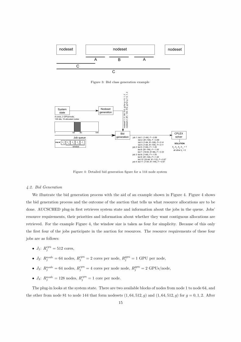
nodeset nodeset
AA B
C
nodeset
C
Figure 3: Bid class generation example
1 64 80 144
System
state
Nodeset
generation
8 cores, 2 GPUs/node,
128 idle, 16 allocated nodes
Job queue
Bid
generation
nodeset 1: (1
, 64, 512
, g)
for
g =
0, 1, 2
nodeset 2: (8
1, 144, 512, g)
for
g =
0, 1, 2
job 1: bid 1: {1-64}, F = 0.89
job 1: bid 2: {81-144}, F = 0.89
job 1: bid 3: {1-64, 81-128}, F= 0.14
job 1: bid 4: {1-64, 81-144}, F= 0.11
job 2: bid 5: {1-64}, F = 1.00
job 1: bid 6: {81-144}, F = 1.00
job 1: bid 7: {16-64, 81-96}, F = 0.33
job 3: bid 8: {1-64}, F = 1.00
job 1: bid 9: {81-144}, F = 1.00
job 1: bid 10: {32-64, 81-112}, F = 0.67
CPLEX
solver
job 4: bid 11: {1-64, 81-144}, F = 0.67
SOLUTION
b4, b
5, b
8, b
11 = 1
all other bi = 0
J5
J4
J3
J2
J1
window
Figure 4: Detailed bid generation figure for a 144 node system
4.2. Bid Generation
We illustrate the bid generation process with the aid of an example shown in Figure 4. Figure 4 shows
the bid generation process and the outcome of the auction that tells us what resource allocations are to be
done. AUCSCHED plug-in first retrieves system state and information about the jobs in the queue. Jobs’
resource requirements, their priorities and information about whether they want contiguous allocations are
retrieved. For the example Figure 4, the window size is taken as four for simplicity. Because of this only
the first four of the jobs participate in the auction for resources. The resource requirements of these four
jobs are as follows:
• J1: Rcpuj = 512 cores,
• J2: Rnodej = 64 nodes, Rcpn
j = 2 cores per node, Rgpuj = 1 GPU per node,
• J3: Rnodej = 64 nodes, Rcpn
j = 4 cores per node node, Rgpuj = 2 GPUs/node,
• J4: Rnodej = 128 nodes, Rcpn
j = 1 core per node.
The plug-in looks at the system state. There are two available blocks of nodes from node 1 to node 64, and
the other from node 81 to node 144 that form nodesets (1, 64, 512, g) and (1, 64, 512, g) for g = 0, 1, 2. After
15

1 64 80 144
J2
J1
J3
J4
t = 0
Figure 5: Allocation by AUCSCHED for the 4 jobs in the queue
the nodesets are created, the AUCSCHED plug-in can now generate possible bid classes. The generated bids
have different preference values, Fjc. Subsection 4.3 explains how preference values are assigned. In general,
we do not enumerate all possible bids. Since each bid appears as a binary variable in the IP solved, such an
act would explode the total number of variables. Hence, it would not be possible to solve our IP problem
within an an acceptable time. In our plug-in there is a variable called MAXBIDSPERJOB which is the
limit on the number of bids generated by our system for each job. In Figure 4, we have shown at most 4
bids generated by the bid generator. The curly brackets next to the bids show the nodes requested by these
bids.
CPLEX Solver [22] takes all bids as the input, and solves the IP problem. In this example, bids b4, b5,
b8 and b11 win the auction. As a result, the following resource allocations are performed:
• J1 is allocated to the nodes {1− 64, 81− 144},
• J2 is allocated to the nodes {1− 64},
• J3 is allocated to the nodes {81− 144},
• J4 is allocated to the nodes {1− 64, 81− 144}.
Figure 5 shows the outcome of this allocation for our AUCSCHED plug-in. it can be seen that this
allocation is the optimal allocation. Figure 6 shows the allocation performed by SLURM’s default backfill
plug-in scheduler, and the consumable resources plug-in for resource selection.
In addition to the type A,B and C bids, we also added an option that would make use of SLURM’s
resource selection plug-in to determine what SLURM’s allocation would be and added this as a bid to each
job’s set of bids. In order to determine the allocation for the second job in the queue, we first update our
node information table as if that job had been scheduled, and let SLURM find its next allocation for the
second job. We refer to these bids as SLURM bids. So our bid generation can be tought of as producing
an enriched set of bids: i.e. bids corresponding to SLURM’s would be allocation and the bids of type A,B
and/or C that we generate.
16

J2
J1
J3
J4
1 64 80 144
1 64 80 144
t = 1
t = 0
Figure 6: Allocation by SLURM’s Backfill plug-in for the 4 jobs in the queue. The pane on top shows the allocation for t = 0,
and pane on bottom shows the allocation for t = 1.
4.3. Fjc Preference Value Calculation
A type A bid can be more desirable than a type B and C bid since it is a contiguous block and is aligned
with another allocated block and hence, may lead to less fragmentation. A type B can be more desirable
than type C, since it is a contiguous block. We are, therefore, motivated to assign preference values in such
a way that FjcA > FjcB > FjcC where cA, cB and cC are respectively type A, B and C bids. We implement
a function that has the following range of values:
FjcC ∈ (0,1
2), FjcB ∈ (
1
2,
3
4), FjcA ∈ (
3
4, 1) (18)
Let Sc denote the set of nodesets from which a bid’s nodes comes from. For type A and B bids, |Sc| = 1.
For type C bids |Sc| > 1. Let S denote the set of all nodesets. The formula used to calculate the preference
value Fjc of a bid c is given as follows:
Fjc = 1.0− k1 − k2 ·|Nc||N |+ 1
− k3 ·|Sc||S|+ 1
(19)
This function together with the constants k1, k2 and k3 are given in Table 9 satisfies the range constraints
given in Equation 18. The idea behind the function is to basically disfavour allocations that are fragmented
or that leads to fragmentation.
Finally we note that SLURM bids are added to the system with coefficients k1 = k2 = k3 = 0, so that all
of them have the highest Fjc values possible. In the next section, we present results from tests that contain
SLURM bids as well tests that do not contain SLURM bids.
5. Workloads and Tests
In order to compare the performance of IPSCHED and AUCSCHED plug-ins with that of SLURM’s
backfill scheduler, we carried out realistic SLURM emulation tests. In emulation tests, we ran an actual
17

Table 9: Constants for Fjc calculation for different job and bid classes
Job type 1
bid type A bid type B bid type C
k1 0 0.25 0.5
k2 0.25 0.25 0.25
k3 0 0 0.25
Job types 2 and 3
bid type A bid type B bid type C
k1 0 0.5 0.5
k2 0 0 0
k3 0 0 0.5
SLURM system and submit jobs to it just like in a real life SLURM usage; the difference being that the jobs
do not carry out any real computation or communication, but rather they just sleep. Such an approach is
more advantageous than testing by simulation since it allows us to test the actual SLURM system rather
than an abstraction of it. Since events are triggered as in actual real life execution, a disadvantage of
emulation approach, however, is the longer time required to complete a test and hence the smaller number
of test runs that can be run. For example, suppose that the next event will happen after 5 seconds. Then
in an event based simulator, the current time variable can be added 5 with an add instruction and the time
variable advances 5 seconds forward instantly whereas in our emulations, actual 5 seconds should elapse
before the next event happens. This then implies a single test may take hours to complete. Note that
even though there are efforts to speed up SLURM emulation tests by intercepting time calls [23], such an
approach will still not be able to speed up our runs. This is because in our IPSCHED and AUCSCHED
plug-ins, at every 5 seconds a scheduling step is invoked which solves an NP-hard problem using CPLEX
[22]. The solver can take as much as 4 seconds. As a result, even if simulation or [23]’s approach is used, the
time taken by a test cannot be reduced. For this reason, we were able to perform a total of 336 tests over
a period of one month with the computational resources available to us. We basically report and discuss
these results.
Our tests have been conducted on a cluster system with 7 nodes with each node having two Intel X5670
6-core 3.20 Ghz CPU’s and 48 GB’s of memory. SLURM was compiled with the enable-frontend mode,
which enables one slurmd daemon to virtually configure various number of nodes.
The following cluster system was emulated in our tests:
• Machine-L : a 1024 node large system with 8 cores and 2 GPUs on each node.
18
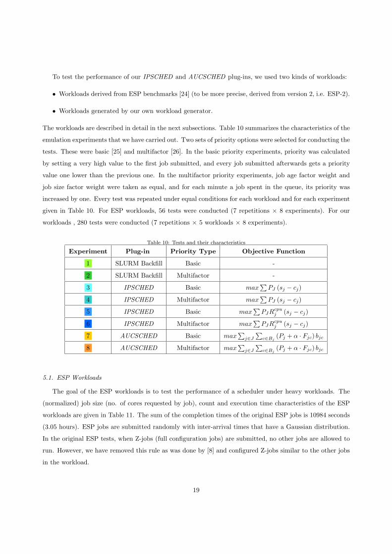
To test the performance of our IPSCHED and AUCSCHED plug-ins, we used two kinds of workloads:
• Workloads derived from ESP benchmarks [24] (to be more precise, derived from version 2, i.e. ESP-2).
• Workloads generated by our own workload generator.
The workloads are described in detail in the next subsections. Table 10 summarizes the characteristics of the
emulation experiments that we have carried out. Two sets of priority options were selected for conducting the
tests. These were basic [25] and multifactor [26]. In the basic priority experiments, priority was calculated
by setting a very high value to the first job submitted, and every job submitted afterwards gets a priority
value one lower than the previous one. In the multifactor priority experiments, job age factor weight and
job size factor weight were taken as equal, and for each minute a job spent in the queue, its priority was
increased by one. Every test was repeated under equal conditions for each workload and for each experiment
given in Table 10. For ESP workloads, 56 tests were conducted (7 repetitions × 8 experiments). For our
workloads , 280 tests were conducted (7 repetitions × 5 workloads × 8 experiments).
Table 10: Tests and their characteristics
Experiment Plug-in Priority Type Objective Function
1 SLURM Backfill Basic -
2 SLURM Backfill Multifactor -
3 IPSCHED Basic max∑PJ (sj − cj)
4 IPSCHED Multifactor max∑PJ (sj − cj)
5 IPSCHED Basic max∑PJR
cpuj (sj − cj)
6 IPSCHED Multifactor max∑PJR
cpuj (sj − cj)
7 AUCSCHED Basic max∑
j∈J∑
c∈Bj(Pj + α · Fjc) bjc
8 AUCSCHED Multifactor max∑
j∈J∑
c∈Bj(Pj + α · Fjc) bjc
5.1. ESP Workloads
The goal of the ESP workloads is to test the performance of a scheduler under heavy workloads. The
(normalized) job size (no. of cores requested by job), count and execution time characteristics of the ESP
workloads are given in Table 11. The sum of the completion times of the original ESP jobs is 10984 seconds
(3.05 hours). ESP jobs are submitted randomly with inter-arrival times that have a Gaussian distribution.
In the original ESP tests, when Z-jobs (full configuration jobs) are submitted, no other jobs are allowed to
run. However, we have removed this rule as was done by [8] and configured Z-jobs similar to the other jobs
in the workload.
19
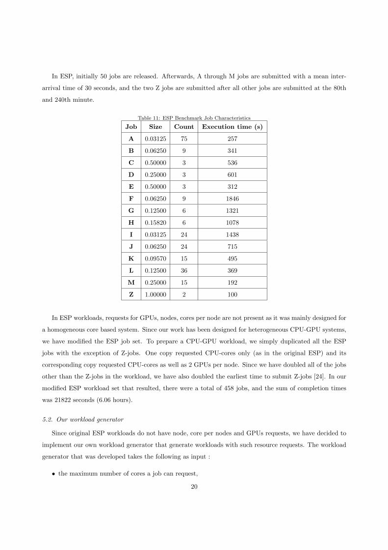
In ESP, initially 50 jobs are released. Afterwards, A through M jobs are submitted with a mean inter-
arrival time of 30 seconds, and the two Z jobs are submitted after all other jobs are submitted at the 80th
and 240th minute.
Table 11: ESP Benchmark Job Characteristics
Job Size Count Execution time (s)
A 0.03125 75 257
B 0.06250 9 341
C 0.50000 3 536
D 0.25000 3 601
E 0.50000 3 312
F 0.06250 9 1846
G 0.12500 6 1321
H 0.15820 6 1078
I 0.03125 24 1438
J 0.06250 24 715
K 0.09570 15 495
L 0.12500 36 369
M 0.25000 15 192
Z 1.00000 2 100
In ESP workloads, requests for GPUs, nodes, cores per node are not present as it was mainly designed for
a homogeneous core based system. Since our work has been designed for heterogeneous CPU-GPU systems,
we have modified the ESP job set. To prepare a CPU-GPU workload, we simply duplicated all the ESP
jobs with the exception of Z-jobs. One copy requested CPU-cores only (as in the original ESP) and its
corresponding copy requested CPU-cores as well as 2 GPUs per node. Since we have doubled all of the jobs
other than the Z-jobs in the workload, we have also doubled the earliest time to submit Z-jobs [24]. In our
modified ESP workload set that resulted, there were a total of 458 jobs, and the sum of completion times
was 21822 seconds (6.06 hours).
5.2. Our workload generator
Since original ESP workloads do not have node, core per nodes and GPUs requests, we have decided to
implement our own workload generator that generate workloads with such resource requests. The workload
generator that was developed takes the following as input :
• the maximum number of cores a job can request,
20
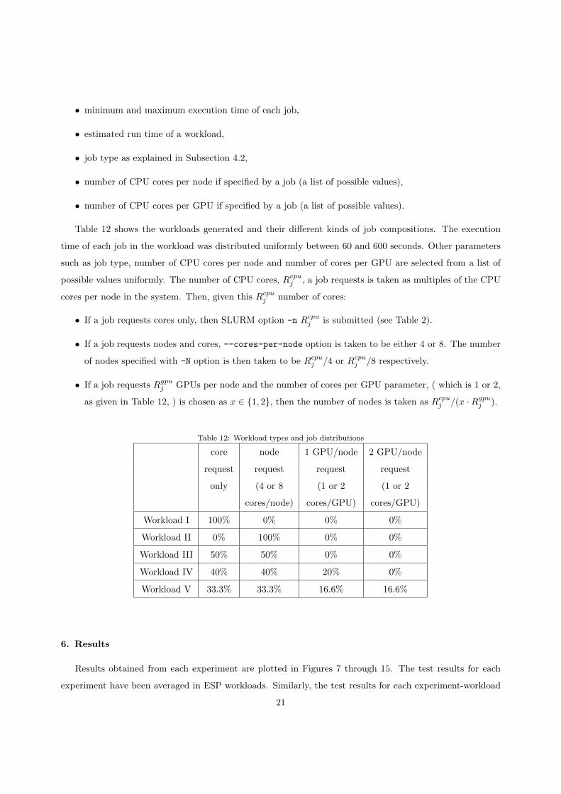
• minimum and maximum execution time of each job,
• estimated run time of a workload,
• job type as explained in Subsection 4.2,
• number of CPU cores per node if specified by a job (a list of possible values),
• number of CPU cores per GPU if specified by a job (a list of possible values).
Table 12 shows the workloads generated and their different kinds of job compositions. The execution
time of each job in the workload was distributed uniformly between 60 and 600 seconds. Other parameters
such as job type, number of CPU cores per node and number of cores per GPU are selected from a list of
possible values uniformly. The number of CPU cores, Rcpuj , a job requests is taken as multiples of the CPU
cores per node in the system. Then, given this Rcpuj number of cores:
• If a job requests cores only, then SLURM option -n Rcpuj is submitted (see Table 2).
• If a job requests nodes and cores, --cores-per-node option is taken to be either 4 or 8. The number
of nodes specified with -N option is then taken to be Rcpuj /4 or Rcpu
j /8 respectively.
• If a job requests Rgpuj GPUs per node and the number of cores per GPU parameter, ( which is 1 or 2,
as given in Table 12, ) is chosen as x ∈ {1, 2}, then the number of nodes is taken as Rcpuj /(x ·Rgpu
j ).
Table 12: Workload types and job distributions
core node 1 GPU/node 2 GPU/node
request request request request
only (4 or 8 (1 or 2 (1 or 2
cores/node) cores/GPU) cores/GPU)
Workload I 100% 0% 0% 0%
Workload II 0% 100% 0% 0%
Workload III 50% 50% 0% 0%
Workload IV 40% 40% 20% 0%
Workload V 33.3% 33.3% 16.6% 16.6%
6. Results
Results obtained from each experiment are plotted in Figures 7 through 15. The test results for each
experiment have been averaged in ESP workloads. Similarly, the test results for each experiment-workload
21
pair have been averaged for our workloads. The results obtained are analyzed using the following performance
measures:
• Utilization: The ratio of the theoretical run-time to the run-time taken by the test. Run-time is the
time it takes to schedule all jobs in workload. Theoretical run-time is taken to be the summation of
duration of each job times its requested core count, all divided by the total number of cores. Note
that this definition of theoretical run-time we use is only a lower bound ; it is not the optimal value.
Computation of the optimal schedule and hence the optimal run-time value is an NP-hard problem.
• Waiting time: The waiting time of each job in the workload, from submission until scheduling.
• Packing Factor: The ratio of the number of nodes a job is allocated to the minimum number of nodes
that job could be allocated into (i.e. packed into).
• Fragmentation: Number of contiguous node blocks allocated to a job.
• Spread: Ratio of the difference between the indices of the last and first nodes plus one to the number
of nodes allocated to a job (assuming node indices start with 1).
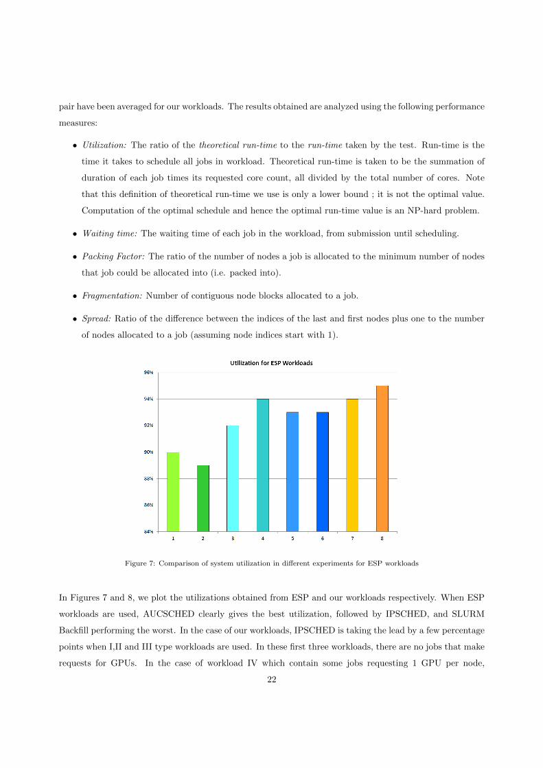
Figure 7: Comparison of system utilization in different experiments for ESP workloads
In Figures 7 and 8, we plot the utilizations obtained from ESP and our workloads respectively. When ESP
workloads are used, AUCSCHED clearly gives the best utilization, followed by IPSCHED, and SLURM
Backfill performing the worst. In the case of our workloads, IPSCHED is taking the lead by a few percentage
points when I,II and III type workloads are used. In these first three workloads, there are no jobs that make
requests for GPUs. In the case of workload IV which contain some jobs requesting 1 GPU per node,
22
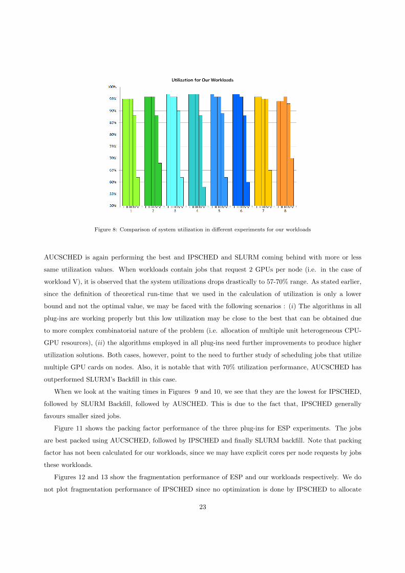
Figure 8: Comparison of system utilization in different experiments for our workloads
AUCSCHED is again performing the best and IPSCHED and SLURM coming behind with more or less
same utilization values. When workloads contain jobs that request 2 GPUs per node (i.e. in the case of
workload V), it is observed that the system utilizations drops drastically to 57-70% range. As stated earlier,
since the definition of theoretical run-time that we used in the calculation of utilization is only a lower
bound and not the optimal value, we may be faced with the following scenarios : (i) The algorithms in all
plug-ins are working properly but this low utilization may be close to the best that can be obtained due
to more complex combinatorial nature of the problem (i.e. allocation of multiple unit heterogeneous CPU-
GPU resources), (ii) the algorithms employed in all plug-ins need further improvements to produce higher
utilization solutions. Both cases, however, point to the need to further study of scheduling jobs that utilize
multiple GPU cards on nodes. Also, it is notable that with 70% utilization performance, AUCSCHED has
outperformed SLURM’s Backfill in this case.
When we look at the waiting times in Figures 9 and 10, we see that they are the lowest for IPSCHED,
followed by SLURM Backfill, followed by AUSCHED. This is due to the fact that, IPSCHED generally
favours smaller sized jobs.
Figure 11 shows the packing factor performance of the three plug-ins for ESP experiments. The jobs
are best packed using AUCSCHED, followed by IPSCHED and finally SLURM backfill. Note that packing
factor has not been calculated for our workloads, since we may have explicit cores per node requests by jobs
these workloads.
Figures 12 and 13 show the fragmentation performance of ESP and our workloads respectively. We do
not plot fragmentation performance of IPSCHED since no optimization is done by IPSCHED to allocate
23

Figure 9: Comparison of job waiting times (in hours) in different experiments for ESP workload
contiguous blocks and hence reduce fragmentation. As the two plots show, SLURM Backfill does a better
job of reducing fragmentation than AUCSCHED in both ESP and our workloads. This is mainly because
SLURM Backfill assigns the jobs on the resources one job at a time, which enables it to place subsequent
jobs with no gaps in between. However, in AUCSCHED, since selected jobs are all simultaneously assigned,
it is possible to have gaps in between placed jobs.
Note there may be cases, where, even though an allocation can be fragmented, (i.e. placed on multiple
blocks), the gaps between the blocks can still be small ; perhaps by one node. In such cases, these multiple
blocks may in fact be close to each other in terms of topological placement (for example by being on the same
communication switch). Hence, a large fragmentation value may not necessarily imply a bad placement for
the purpose of communication. Spread measure allows us to look into this kind of separation on allocations.
As seen in plots in Figures 14 and 15, AUCSCHED is doing a better job of reducing the spread in allocations.
We do not again report spread performance of IPSCHED since no special optimization was done by it to
reduce spread.
7. Discussion and Conclusions
The work presented in this paper (i) shed light onto some unknown issues about use of IP packages like
CPLEX in a real large-scale job scheduler system (ii) contributed new job scheduling algorithms and software
as well as (iii) pointed to new problems to investigate within the context of state-of-the-art heterogeneous
clusters. The findings and contributions can be summarized as follows:
24
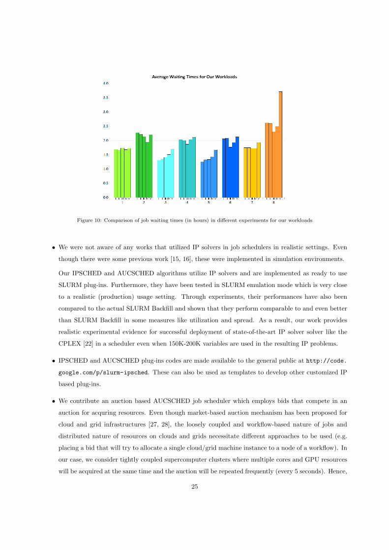
Figure 10: Comparison of job waiting times (in hours) in different experiments for our workloads
• We were not aware of any works that utilized IP solvers in job schedulers in realistic settings. Even
though there were some previous work [15, 16], these were implemented in simulation environments.
Our IPSCHED and AUCSCHED algorithms utilize IP solvers and are implemented as ready to use
SLURM plug-ins. Furthermore, they have been tested in SLURM emulation mode which is very close
to a realistic (production) usage setting. Through experiments, their performances have also been
compared to the actual SLURM Backfill and shown that they perform comparable to and even better
than SLURM Backfill in some measures like utilization and spread. As a result, our work provides
realistic experimental evidence for successful deployment of state-of-the-art IP solver solver like the
CPLEX [22] in a scheduler even when 150K-200K variables are used in the resulting IP problems.
• IPSCHED and AUCSCHED plug-ins codes are made available to the general public at http://code.
google.com/p/slurm-ipsched. These can also be used as templates to develop other customized IP
based plug-ins.
• We contribute an auction based AUCSCHED job scheduler which employs bids that compete in an
auction for acquring resources. Even though market-based auction mechanism has been proposed for
cloud and grid infrastructures [27, 28], the loosely coupled and workflow-based nature of jobs and
distributed nature of resources on clouds and grids necessitate different approaches to be used (e.g.
placing a bid that will try to allocate a single cloud/grid machine instance to a node of a workflow). In
our case, we consider tightly coupled supercomputer clusters where multiple cores and GPU resources
will be acquired at the same time and the auction will be repeated frequently (every 5 seconds). Hence,
25

Figure 11: Comparison of job packing factors in different experiments for ESP workload
we are required to solve a far more complex combinatorial optimization problem in a very short period
of time. To the best of our knowledge, our AUCSCHED is probably the first auction based scheduler
that has been developed for clusters.
In the future, we will work on the following:
• Identify the causes of the low system utilizations in workloads containing jobs that use multiple GPU
cards and offer remedies for them.
• Improve the performance of AUCSCHED algorithm by developing more IP formulations that will
enable us to increase the number of bids generated for each job.
• Build a publicly accessible CPU-GPU workload archive.
26
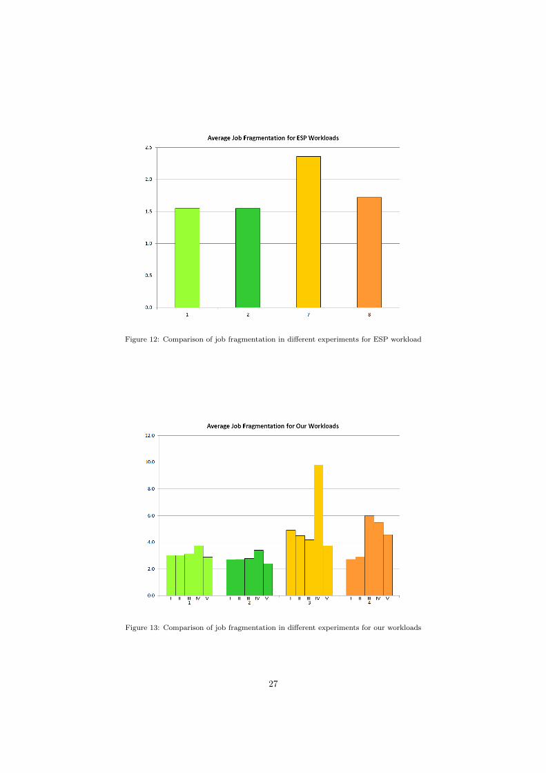
Figure 12: Comparison of job fragmentation in different experiments for ESP workload
Figure 13: Comparison of job fragmentation in different experiments for our workloads
27

Figure 14: Comparison of job spread in different experiments for ESP workload
Figure 15: Comparison of job spread in different scheduling mechanisms for our workloads
28
8. Acknowledgments
This work was financially supported by the PRACE project funded in part by the EUs 7th Framework
Programme (FP7/2007-2013) under grant agreement no. RI-211528 and FP7-261557. We thank Matthieu
Hautreux from CEA, France, for discussions and his help during the implementation of our plug-in. The
authors have used the Bogazici University Polymer Research Center’s cluster (funded by DPT project
2009K120520).
References
[1] A. Yoo, M. Jette, M. Grondona, SLURM: Simple Linux Utility for Resource Management, in: Job Scheduling Strategies
for Parallel Processing, vol. 2862 of Lecture Notes in Computer Science, ISBN 978-3-540-20405-3, 2003.
[2] Moab Workload Manager Documentation, URL http://docs.adaptivecomputing.com/, 2012.
[3] B. Bode, D. M. Halstead, R. Kendall, Z. Lei, D. Jackson, The portable batch scheduler and the maui scheduler on linux
clusters, in: Proceedings of the 4th annual Linux Showcase & Conference - Volume 4, ALS’00, USENIX Association,
Berkeley, CA, USA, 27–27, URL http://dl.acm.org/citation.cfm?id=1268379.1268406, 2000.
[4] LSF (Load Sharing Facility) Features and Documentation, URL http://www-03.ibm.com/systems/technicalcomputing/
platformcomputing/products/lsf/index.html, 2012.
[5] Slurm Used on the Fastest of the TOP500 Supercomputers, URL http://www.hpcwire.com/hpcwire/2012-11-21/slurm_
used_on_the_fastest_of_the_top500_supercomputers, 2012.
[6] S. Martello, P. Toth, Knapsack problems: algorithms and computer implementations, Wiley-Interscience series in discrete
mathematics and optimization, J. Wiley & Sons, ISBN 9780471924203, 1990.
[7] Slurm Documentation, URL http://www.schedmd.com/slurmdocs, 2012.
[8] Y. Georgiou, Contributions For Resource and Job Management in High Performance Computing, Ph.D. thesis, Universite
de Grenoble, France, 2010.
[9] in: Grid Resource Management, vol. 64 of International Series in Operations Research & Management Science, ISBN
978-1-4020-7575-9, 2003.
[10] Torque Resource Manager Documentation, URL http://docs.adaptivecomputing.com/, 2012.
[11] I. Redbooks, Workload Management With Loadleveler, Vervante, ISBN 9780738422091, 2001.
[12] T. Tannenbaum, D. Wright, K. Miller, M. Livny, Beowulf cluster computing with Linux, chap. Condor: a distributed job
scheduler, ISBN 0-262-69274-0, 307–350, 2002.
[13] N. Capit, G. Da Costa, Y. Georgiou, G. Huard, C. Martin, G. Mounie, P. Neyron, O. Richard, A batch scheduler with
high level components, in: Proceedings of the Fifth IEEE International Symposium on Cluster Computing and the Grid
(CCGrid’05) - Volume 2 - Volume 02, CCGRID ’05, ISBN 0-7803-9074-1, 776–783, 2005.
[14] W. Gentzsch, Sun Grid Engine: towards creating a compute power grid, in: Cluster Computing and the Grid, 2001.
Proceedings. First IEEE/ACM International Symposium on, 35 –36, 2001.
[15] M. Etinski, J. Corbalan, J. Labarta, M. Valero, Linear programming based parallel job scheduling for power constrained
systems, in: High Performance Computing and Simulation (HPCS), 2011 International Conference on, 72 –80, 2011.
[16] O. Erbas, C. Ozturan, Collective Match-Making Heuristics for Grid Resource Scheduling, in: High Performance Grid
Middleware, Brasov, Romania, 2007.
[17] A. H. Ozer, C. Ozturan, A model and heuristic algorithms for multi-unit nondiscriminatory combinatorial auction, Comput.
Oper. Res. 36 (1) (2009) 196–208, ISSN 0305-0548.
29

[18] J. A. Pascual, J. Navaridas, J. Miguel-Alonso, Job Scheduling Strategies for Parallel Processing, chap. Effects of Topology-
Aware Allocation Policies on Scheduling Performance, ISBN 978-3-642-04632-2, 138–156, 2009.
[19] F. J. Ridruejo Perez, J. Miguel-Alonso, INSEE: an interconnection network simulation and evaluation environment, in:
Proceedings of the 11th international Euro-Par conference on Parallel Processing, Euro-Par’05, ISBN 3-540-28700-0, 978-
3-540-28700-1, 1014–1023, 2005.
[20] D. Feitelson, Parallel workloads archive, URL http://www.cs.huji.ac.il/labs/parallel/workload, 2005.
[21] S. Soner, C. Ozturan, Integer Programming Based Heterogeneous CPU-GPU Cluster Scheduler for SLURM Resource
Manager, in: HPCC-ICESS, 2012.
[22] IBM ILOG CPLEX Optimizer, URL http://www-01.ibm.com/software/integration/optimization/cplex-optimizer/,
2012.
[23] A. Lucero, Simulation of batch scheduling using real production-ready software tools, 2011.
[24] A. Wong, L. Oliker, W. Kramer, T. Kaltz, D. Bailey, ESP: A System Utilization Benchmark, in: Supercomputing,
ACM/IEEE 2000 Conference, 15, 2000.
[25] SLURM Priority Plugin API, Slurm Documentation, URL https://computing.llnl.gov/linux/slurm/priority_
plugins.html, 2012.
[26] Multifactor Priority Plugin, Slurm Documentation, URL https://computing.llnl.gov/linux/slurm/priority_
multifactor.html, 2012.
[27] B. M. Harchol, Auction based scheduling for the TeraGrid, URL http://www.cs.cmu.edu/~harchol/teragrid.pdf, 2007.
[28] R. Prodan, M. Wieczorek, H. M. Fard, Double Auction-based Scheduling of Scientific Applications in Distributed Grid
and Cloud Environments, J. Grid Comput. (2011) 531–548.
30