integrated design and manufacturing for the high speed ... · integrated design and manufacturing...
TRANSCRIPT

NA 5A-CR-1 9718 3 NASw-4435
Integrated Design andManufacturing for the High Speed
Civil Transport
Preliminary Design Methodology an_ _
Optimization for an HSCT Nacelle/WingConfiguration
Final Report
NASA USRA Advanced Design PrograrrAeronautics
School of Aerospace EngieeringGeorgia Institute of Technology
Atlanta, GA, June 1994
Z
uJ
Q,-,
uJ
ZC_b-, _i.
r._ _...__r,,"
I".- I--(_-
I
_Z
(/)_(_i i
t.=00.
0r.-
0-,== o',
C
_'2
C_t,-_k
Z G
uJ _)
t_,_
0
https://ntrs.nasa.gov/search.jsp?R=19950006287 2018-06-22T19:36:02+00:00Z

Abstract
In June 1992, the School of Aerospace Engineering at Georgia Tech was awarded a
three year NASA University Space Research Association (USRA) Advanced Design
Program (ADP) grant to address issues associated with the Integrated Design and
Manufacturing of High Speed Civil Transport (HSCT) configurations in its graduate
Aerospace Systems Design courses. This report provides an overview of the on-going
Georgia Tech initiative to address these design/manufacturing issues during the preliminary
design phases of an HSCT concept. The new design methodology presented here has been
incorporated in the graduate aerospace design curriculum and is based on the concept of
Integrated Product and Process Development (IPPD). The selection of the HSCT as a pilot
project was motivated by its potential global transportation payoffs, its technological,
environmental, and economic challenges, and its impact on U.S. global competitiveness.
This pilot project was the focus of each of the five design courses that form the graduate
level aerospace systems design curriculum. This year's main objective was the
development of a systematic approach to preliminary design and optimization and its
implementation to an HSCT wing/propulsion configuration. The new methodology, based
on the Taguchi Parameter Design Optimization Method (PDOM), was established and was
used to carry out a parametric study where various feasible alternative configurations were
evaluated. The comparison criterion selected for this evaluation was the economic impact
of this aircraft, measured in terms of average yield per Revenue Passenger Mile ($/RPM) 1.

Table of Contents
1.0 Introduction ................................................................................... 1
2.0 Georgia Tech's IPPD Methodology ........................................................ 32.1 Implementation of IPPD Methodology ............................................... 6
2.1.1 Establishing the Need .......................................................... 62.1.2 Def'ming the Problem ........................................................... 7
2.1.2.1 HSCT Customer Requirements ....................................... 72.1.2.2 Key Product and Process Characteristics ............................ 9
2.1.2.2.1 Aerodynamics and Performance .............................. 102.1.2.2.2 Propulsion ...................................................... 122.1.2.2.3 Structural Analysis & Materials .............................. 142.1.2.2.4 Advanced Flight Systems and Control ...................... 142.1.2.2.5 Life Cycle Costs ................................................ 152.1.2.2.6 Manufacturing .................................................. 16
2.1.2.3 Formation of the Interrelationship Digraph and the
N 2 Diagram ............................................................. 242.1.2.4 QFD - Product Planning Matrix ...................................... 262.1.2.5 Results of Product Planning Matrix ................................. 28
2.1.3 Establishing Value Objectives ................................................ 292.1.3.1 Feasibility Constraints ................................................. 32
2.1.3.2 Life Cycle Cost Matrix ................................................ 322.1.3.3 Average Yield per Revenue Passenger Mile ($/RPM) ............. 35
2.1.4 Generation of Feasible Alternatives .......................................... 35
2.1.4.1 Baseline Configuration ................................................ 352.1.4.2 Stability and Control of Baseline Configuration ................... 372.1.4.3 Taguchi Parameter Design Optimization Methods (PDOM) ...... 472.1.4.4 Aircraft LCC Analysis and Synthesis Simulation Method ........ 502.1.4.5 Test of Economic Analysis on the Baseline ......................... 51
2.1.4.5.1 Simulation Interpretation ...................................... 542.1.4.5.2 The Experiment ................................................. 552.1.4.5.3 Result Interpretation ........................................... 572.1.4.5.4 Confurnation Test .............................................. 61
2.1.4.6 Top Level Orthogonal Array .......................................... 622.1.5 Evaluation of Alternatives ..................................................... 62
2.1.5.1 Aerodynamics Orthogonal Array ..................................... 642.1.5.2 Aerodynamics, Structures, and Manufacturing Opt. Wing ....... 68
2.1.5.2.1 Combined Array: Response-model/combined-arrayApproach to Nacelle-Wing-Fuselage Integration ........... 68
2.1.5.2.2 Limitations of Taguchi Method ............................... 692.1.5.2.3 Limitations of Two-Part Experimentation Strategy ........ 692.1.5.2.4 Limitations of the Loss-Model Approach ................... 702.1.5.2.5 The Use of Response-Model/Combined-Array
Approach ........................................................ 712.1.5.2.6 Implementation Procedure of the Combined Array
Experiment for the Nacelle-Wing-Fuselage Integration... 722.1.5.3 Manufacturing Implementation ....................................... 762.1.5.4 Synthesis/Propulsion/Economic Analysis ......................... 78
2.1.6 Making a Decision ............................................................. 813.0 Conclusion - Future Work ................................................................. 83
4.0 Appendix A .................................................................................. 855.0 References .................................................................................... 88
ii
List of Figures
Figure 1Figure 2Figure 3Figure 4Figure 5Figure 6Figure 7Figure 8Figure 9Figure 10Figure 11Figure 12Figure 13
Figure 14
Figure 15Figure 16Figure 17
Figure 18
Figure 19Figure 20Figure 21Figure 22Figure 23Figure 24Figure 25Figure 26Figure 27Figure 28Figure 29Figure 30Figure 31Figure 32Figure 33Figure 34Figure 35Figure 36Figure 37Figure 38Figure 39Figure 40Figure 41
Figure 42
Figure 43
Figure 44
Figure 45
Georgia Tech's Team Activity Network Diagram ................................ 3Integrated Product and Process Development Approach ........................ 4Interaction of the Four Key Elements in Concurrent Engineering .............. 5Affinity Diagram: Voice of the Customer .......................................... 7Customer Requirements ............................................................. 9Key Product and Process Characteristics ......................................... 10CATIA Model of the Mixed Flow TurboFan .................................... 13
CATIA Model of a Turbine Bypass Engine ...................................... 13Description of Superplastic Forming Process .................................... 20Powder Metallurgy Process ........................................................ 22Interrelationship Digraph of the Key Product and Process Characteristics... 25NxN Diagram for Key Product and Process Characteristics ................... 26QFD Matrix Relating the Key Product and Process Characteristics to theCustomer Requirements ............................................................ 27Prioritization Man'ix Showing the Influence of the Key Product andProcess Characteristics on Each Other ............................................ 28Return on Investment Criteria ...................................................... 29
Interrelationship Digraph of the ROI Criteria .................................... 30QFD Matrix Relating the ROI Criteria to the Key Product and ProcessCharacteristics ....................................................................... 31
When LCC are Rendered Unchangeable Versus When LCC are ActuallyExpended for a Given Design ...................................................... 33The QFD Matrix Relating the ROI to the Cost Drivers .......................... 34Baseline Mission Profile ............................................................ 36
Georgia Tech's HSCT Double-Delta Baseline Configuration .................. 36APAS HSCT Baseline Configuration ............................................. 38Case 1 - Cm @ Mach ---0.95 ...................................................... 39Case 1 - Cm @ Mach- 2.4 ....................................................... 40Case 1 - Crn0t @ Mach -- 2.4 & 0.95 ............................................ 40Case 2 - Cm @ Mach -- 0.95 ...................................................... 41Case 2 - Cm @ Math - 2.4 ....................................................... 41Case 2 - Cmct @ Mach -- 2.4 & 0.95 ............................................ 42Case 1 -Cn @ Math = 0.95 ....................................................... 43Case 1 - Cn @ Math - 2.4 ........................................................ 43Case 2-Cn @ Math -- 0.95 ....................................................... 44Case 2 - Cn @ Maeh = 2.4 ........................................................ 44Case 1 - C! @Mach -- 0.95 ....................................................... 45Case 1 -C1 @ Mach --- 2.4 ......................................................... 46Case 2 - (21@ Mach - 0.95 ...................................................... 46Case 2-CI @ Math -- 2.4 ......................................................... 47
HSCT Economic Sensitivity Assessment Methodology ........................ 48The Taguchi Method Flow Chart .................................................. 49ALCCA Flowchart .................................................................. 51
Complexity Factors ................................................................. 53$/RPM Variations for All Experiments Performed Including the"Optimum" Distribution ............................................................ 58Control Factor Influences on Average Yield / Revenue Passenger Mile($/RPM) ...................................................................... . ....... 59
Aircraft Acquisition Price Variation for the "Optimum" and "Worst"Conditions ........................................................................... 60
Average Ticket Price Variation for the "Optimum" and "Worst"Conditions ............................................................................ 60
$/RPM Variation for the "Optimum" and "Worst" Conditions ................ 61
lU

Figure 46Figure 47Figure 48Figure 49Figure 50Figure 51Figure 52Figure 53Figure 54
Figure 55
List of Figures (Cont.)
Feasible Alternative Evaluation Flowchart ....................................... 63
Wing Optimization Procedure ...................................................... 64Wing Planform Configuration ..................................................... 65Control Factor Influences on the L/D Ratio for a Supersonic Mission ........ 67Two-Part Experimentation Strategy for Robust Design ........................ 70Combined Orthogonal Array ....................................................... 73
Wing Manufacturing Consideration, Three Point Design ...................... 75Significant Control Factor Influences on the System OEC, $/RPM ........... 80$/RPM Variations for the First Feasible Configuration of the Top LevelOrthogonal Array Including the "Optimum" Distribution .................. . .... 80Concept Evaluation Experimental Schematic ..................................... 82
iv

TableITable IITable 111
Table IVTable VTable VITable VIITable VIIITable IXTable X
Table XITable XIITable XII1Table XIVTable XVTable XVITable XVII
Table XVM
Table XIXTable XXTable XXITable XXII
SPD/DB Cost Reduction Potential .............................................. 21
Process Manufacturing Requirements and Costs .............................. 23Suitability of Manufacturing Processes to AlternativeManufacturing Forms ............................................................. 24Return on Investment for Airlines and Manufacturers ........................ 33
Baseline Configuration Descriptions ............................................ 37Economic Sensitivity Analysis Ground Rules and Assumptions ............ 52Control Factors as They Relate to the ALCCA Program ..................... 54Noise Factors as They Relate to the ALCCA Program ....................... 54The Complete Orthogonal Array for the Design of Experiments ............ 56The Optimal Configuration for the "Smallerthe Better" Quality Characteristic Case ......................................... 58Change in Average Yield per RPM from the "Optimum" Condition ........ 61The "Optimum" Condition Confirmation Results ............................. 61Top-Level Decision OA .......................................................... 62Aerodynamic Experiment Control Factors ..................................... 66Aerodynamic Experiment Noise Factors ....................................... 66Optimal Aerodynamic Control Factor Levels ................................. 67Structure/Aerodynamics/Material/Manufacturing Combined Controland Noise Factors ................................................................. 73Material Selection ................................................................. 75
Manufacturing Full Factorial Experiment ...................................... 77Propulsion/Sizing/Economic Experiment Control Factors ................... 78
Propulsion/Sizing/Economic Experiment Noise Factors ..................... 79"Optimal" Control Factor Settings .............................................. 79
V

Forward
This report documents work completed during the second year for the NASAUniversity Space Research Association (USRA) Advanced Design Program (ADP) inAeronautics at the Georgia Institute of Technology. Professor Daniel Schrage, ProfessorJames Craig, and Dr. Dimitri Mavris were the coordinators of this project. Variousmembers of the Aerospace Systems Design Laboratory (ASDL) at Georgia tech providedhelpful suggestions, especially Mark Hale, Peter Rohl, Bill Marx, and Dan DeLaurentis.Jason Brewer and Craig Mueller were the team leaders. The design team consisted of thefollowing members and their corresponding areas of expertise and computational tools inparentheses used where appropriate:
Aerodynamics (BDAP)
Structures (ASTROS)
Materials
Stability & Control (APAS)
Propulsion (QNEP/FLOPS)
Manufacturing (MTT)
Synthesis/Sizing (FLOPS)
Geometry (CADAM/CATIA)
Robust Design Optimization(Taguchi/MDO/QT4)
Life Cycle Cost (ALCCA)
Jae Moon Lee, Anurag Gupta
Craig Mueller, Monica Morrisette
Monica Morrisette
John Dec
Jason Brewer, Kevin Donofrio
Hilton Sturisky and Doug Smick
Craig Mueller, Jason Brewer
Kevin Donofrio, Meng Lin An
Jason Brewer, Wei Chen, Meng Lin An
Jason Brewer
COPYRIGHT © 1994 GEORGIA INSTITUTE OF TECHNOLOGY,SCHOOL OF AEROSPACE ENGINEERING
PERMISSION TO REPRODUCE THIS DOCUMENT OR ANY PART OF ITS CONTENTS MUST BEACQUIRED FROM:
PROFESSOR DANIEL P. SCHRAGESCHOOL OF AEROSPACE ENGINEERINGGEORGIA INSTITLrl'E OF IK-'HNOLOGY
ATLANTA, GEORGIA 30332-0150
vi
1.0 Introduction
Under the University Space Research Association (USRA) Advanced Design
Program (ADP), the School of Aerospace Engineering at Georgia Tech has undertaken the
initiative of integrating aircraft design and manufacturing, and incorporating it in their
design curriculum at the graduate level. The faculty at Georgia Tech have felt that in order
to carry out this objective, a highly focused program was needed. NASA's High Speed
_h (HSR) program provided one such opportunity. Under this program, NASA and
this country's aerospace industry have undertaken the challenge of developing the
technology by the turn of the century which will allow the launch of a High Speed Civil
Transport (HSCT) aircraft capable of cruising at a Mach number of 2.0 or greater and
carrying 300 passengers to destinations in excess of 5,000 nautical miles.
A HSCT is being designed as a commercial supersonic transport vehicle that will be
used in portions of the international market. This HSCT must not only be environmentally
friendly (e.g. abide by FAR Stage HI noise regulations, reduce or eliminate sonic boom
over land associated with supersonic flight, and reduce NOx emissions that are harmful to
the ozone layer), but it must also be economically competitive with current and projected
long range subsonic fleet (i.e. Boeing 747-400). Market surveys have indicated that a
significant increase in ticket price will have an adverse effect on passenger demand;
however, there have been indications that most passengers would be willing to pay a
premium for supersonic flight (up to 30% more than subsonic transport ticket fares). A
ticket price above this level will most likely reduce the total market demand to a point where
airlines and aircraft manufacturers might not be willing to make a commitment to buy or to
undertake the aircraft production 2. Therefore, in order to ensure the production of a
HSCT, it is essential to maintain an affordable ticket fare for the passenger, while retaining
a reasonable Return on Investment (ROD for both the airline and the airframe/engine
manufacturers.
This initiative is full of technological challenges affecting each and every one of the
various disciplines involved (Aerodynamics, Structures, Propulsion, Manufacturing, etc.).
It is because of these challenges, as well as the overall relevance and importance of this
project to our industry and nation, that this aircraft was chosen to be the focus of this
investigation.
A number of graduate and senior elective courses were used to introduce the
students to appropriate design and manufacturing methods. The School of Aerospace
Engineering has a strong educational program in design, consisting of five graduate level
courses (Concurrent Engineering, Introduction to Life Cycle Cost, Introduction to
Computer Aided Design, and Aerospace Systems Design I & ]I)3, that have been

continuously improved and influenced by advances made on the research side of the
program. An Aerospace Systems Design Laboratory (ASDL) has been developed to
support this program.
During the first year of this three year program, the overall design methodology
was developed and tested (paper and report presented in USRA's 1993 ADP Summer
Conference4). In this second year, the methodology has been applied to two of the most
critical components of the aircraft - the propulsion system and the wing. This year's
graduate student team identified the customer requirements and the key product and process
characteristics, generated a baseline configuration, and proceeded with the implementation
of Georgia Tech's preliminary design methodology.
Once the baseline was established, the team was divided into multidisciplinary
groups that performed a Nacelle-Wing-Fuselage integration analysis, addressing issues
related to aerodynamics, structures, and manufacturing of the wing, as well as a propulsion
system down selection study. The results of all these studies were then incorporated back
into a system synthesis code (FLight OPtimization System (FLOPS)) 5 in order to modify
the baseline configuration and generate a new "optimum" configuration. This "optimum"
configuration had to be able to satisfy all design requirements and constraints and was used
to assess the economic affordability of this aircraft. Furthermore, a robust design
assessment of the configuration provided some indication of the risk associated with the
various assumptions and decisions made throughout the design process. This analysis was
based on a risk analysis/control/reduction technique called the Taguchi Parameter Design
Optimization Method (PDOM). While the Taguchi PDOM has been utilized for robust
design of parts, components, and some systems, it is believed that its use in this exercise is
unique and offers considerable promise for Integrated Product and Process Development
(IPPD). The tasks performed by the team can best be presented by an activity network
diagram, one of the Seven Management and Planning Tools that will be discussed later. It
is presented in Figure 1 and illustrates the sequence of events that took place over this nine
month period.

W_I W_3 We.k6 W_IOWeek 14 We117
I_mdj_y Imp_
I p hi,t, , •7 Dip
Wink21 Week 22 Woek 5'qW_ W_3I W_33
Figure 1 : Georgia Tech's Team Activity Network Diagram
2.0 Georgia Tech's IPPD Methodology
The design curriculum at Georgia Tech follows closely an Integrated Product and
Process Development or Concurrent Engineering (CE) approach. Since most of the
students entering the design course sequence are unaware of what Concurrent Engineering
is, an entire course dedicated to the methodology and tools behind it is offered to provide
them with all the necessary team building and brainstorming skills that were used
throughout this investigation.
3

Concurrent Engineering is commonly def'med as the "systematic approach to the
integrated, concurrent design of products and their related processes 6". This method
provided a means for the team to brainstorm up front and understand the customer
requirements. Furthermore, CE provides the tools needed to integrate manufacturing and
operation support into product design, and it allows the designers to confront potential
problems in the early design stages when the system is still flexible enough to be altered.
This approach increases the initial effort and time needed for the early design stages, but
produces significant cost and time savings in downstream activities and leads to a more
efficient and effective design.
DESIGN(SYSTEM)
DESIGN DEStGN
INTEGRATEDCOMPONENT PRODUCT- COMPONENT
TRADES PROCESS TRADESDEVELOPMENT
DEs. T /:s DEs.
Figure 2: Integrated Product and Process Development Approach
The methodology currendy used in the graduate design program is illustrated in
Figures 2 and 3. The flow diagram for IPPD, presented in Fig. 2, illustrates the
hierarchical decomposition activities from the conceptual design phase (system level), to
preliminary design (major component/sub-system), to detailed design (part/sub-component
level), and to manufacturing. The inner small loops on the right half represent the
design wade iterations. The left half shows the process recomposition activities, and the
4

inner loops represent the _ design trades. The long outer loop iteration represents
what has usually been done in the past when redesign was often required due to product
design incompatibilities with manufacturing processes. What is desired with IPPD is the
ability to make parallel I/XOdaf.I:l_,._f_ design trades at the system level, as well as the
component and part level.
While Fig. 2 represents the flow process desired for IPPD, it does not provide the
methodology W.xluired to implement IPPD and make the parallel product-process design
trades. The methodology being developed and utilized at Georgia Tech is illustrated in Fig.
3. Industry has confirmed that, in a genetic manner, this approach is very similar to the
IPPD methodologies they are also trying to develop and implement.
_MPUTER-INTEGR ATED ENVIRGN ME NT_=_=_=_-..,_
rO_WN DES_N / ...... SYSrEyS--DECISION SUPPORT PROCESS / EN(_INEEFIlNG ME]HODS "%k
zt 0_ k
I I IENGINEERING &
Figure 3: Interaction of the Four Key Elements In Concurrent Engineering
This methodology provides the desired systematic approach to the integrated,
concurrent design of products and their related processes, including manufacturing and
support. Figure 3 illustrates the interaction of the four key elements necessary for parallel
product and process trades to be made at the appropriate level of system decomposition and
recomposition. Depicted is an "umbrella" with the four key elements: systems engineering
methods, quality engineering methods, top down design decision support process, and
computer integrated environment. The interaction among these elements to make parallel
product and process design trades is shown below the "umbrella". The top down design
decision support process usually starts by establishing the need and proceeds by def'ming

the problem, establishing the value objectives, generating feasible alternatives, evaluating
these alternatives, and reaching a final decision. Quality engineering methods include the
use of Quality Function Deployment, Taguchi methods, and Statistical Process Control.
Systems engineering methods include system decomposition, functional allocation, and
system synthesis. Finally, the computer-aided environment provides a means of
integrating these processes together. The methodology takes advantages of methods and
tools, such as the Seven Management and Planning Tools, requirement and functional
analysis, decomposition, etc. for both product and process. System synthesis is achieved
through the use of Multidiseiplinary Design Optimization (MDO) and robustness of design
methods to evaluate the generated feasible alternatives. This way, the best alternative based
on the criteria established from the value objectives is made.
2.1 Implementation of IPPD Methodology
2.1.1 Establishing the Need
The introduction of a HSCT in the long range, transcontinental air travel market is
becoming increasingly more appealing to the aerospace industry as market forecasts project
that world air travel will almost double by the year 2000. A need for an aircraft that could
provide passengers with a significantly reduced travel time (approximately 45%) to
destinations in the 5,000 - 6,500 nmi range appears to exist, provided that a fare
competitive with subsonic aircraft can be achieved. This range covers the long routes of
the international market including the Pacific rim where most of the travel demand increases
are expected. In order for such a concept to be economically competitive with current long
range subsonic aircraft similar in size to the Boeing 747-400, it is imperative that the turn-
around time on the ground must be reduced so as to complete two round trips daily 2.
Therefore, only enfise speeds between Mach 2.0 and 2.6 are currently being considered,
since speeds greater than Mach 2.6 would require special fuels. In addition, this HSCT
will have to be able to carry 280-320 passengers in order to reduce the average yield per
Revenue Passenger Mile, $/RPM. The $/RPM is a metric that captures the Return on
Investment (ROI) concerns of both the airline and the manufacturer and can be easily
translated to ticket price fares once the occupancy load factors are known. Finally, the
aircraft must be compatible with current airports (i.e. take-off and landing field length
distances, terminals, etc.).
6

2.1.2 Defining the Problem
Concurrent engineering techniques are implemented at this point in order to better
understand the challenges faced by a HSCT. This task is achieved through the use of a
series of QuaLity Function Deployment (QFD) matrices. Construction of a QFD matrix is
accomplished using such methods as the Seven Management and Planning Tools and a
functional analysis method, the N 2 diagram, which is incorporated to better organize the
requirements of the different system products and their related processes. The Georgia
Tech IPPD methodology employs these tools to generate a product planning matrix,
establish a value objectives matrix, and identify all feasibility constraints. These Seven
Management and Planning Tools include such brainstorming tools as the affinity and tree
diagrams, the interrelationship digraph, and the prioritization and relationship matrices.
Once a product planning matrix is developed, the remaining tools, the activity network
diagram and the process decision program chart are used to layout the implementation and
deployment of the product planning matrix. The affinity and tree diagrams were used
extensively by the HSCT team as brainstorming techniques to identify the customer
requirements and the key product and process characteristics.
2.1.2.1 HSCT Customer Requirements
A QFD approach was used to relate the customer's requirements to the key product
and process characteristics. The customer requirements are established through the use of
an affinity diagram by compiling a list of possible customers and attempting to define their
requirements and concerns for a HSCT as seen in Figure 4. These customers included the
airlines, passengers, environmental groups/agencies, and the Federal Aviation
Administration(FAA).
• _, Mainmum_,& Acqu_tioaCost
• Rmp, Bbck Sl,_d
• FastTurn Around Tram
• _ TYl_llZfficimcy
• Raturnem Inv_4mm_
•_ omv_'Q_y
• Paylamd_,F_ Space
• Hi_ LU_Spm
Figure 4:
[mwtalim
Ir
• NOx _mlmiana
* Ozzm I)q, ld_m
• Mmulactming P_ulion
• TIO & l._ding No_e
W_
._,_
[Gov_t (FAA) [
Ir _c_n_t&_ -_
° _ (_)
* /rre Resis_at _
• Crmh W_
• _A_Ru C.ap_i_/, NewL •
Ir- •
• Ticket Prices
•s,_-ty
• fw.at Size & f,padng
• Cat_ No_ & I-l_t
• ScheduleReliability
• u_o,, (T_hone)
Affinity Diagram: Voice of the Customer7

Affordability related issues pose the biggest challenge for a HSCT concept. The
airlines, the HSCT's primary customer, facing serious financial problems, will be very
reluctant to purchase such a vehicle if the potential for a high return on investment is not
feasible. This means that the acquisition and total operating costs must be kept low, and
the generated revenues must be as high as possible while maintaining low ticket fares. In
order to generate significant revenues, a HSCT will need to capture a major portion of the
overseas market. This can be done by reducing time on long range flights by 45% and
keeping fares competitive with subsonic transports similar in size to the 747-400. The
aircraft must be compatible with existing airports, have a quick turn-around time, use
conventional fuels, and keep maintenance costs low.
As mentioned previously, the passenger expects fares which are comparable to
subsonic transport fares. The passenger also requires a level of comfort while flying,
including aspects such as low cabin noise, comfortable seating, suitable temperature, and
smooth flying. Because a HSCT will be most appealing to business flyers, the aircraft
must have a reliable schedule, which implies that it must have a high dispatch reliability and
be easy to maintain and quick to service in case of any unexpected occurrences.
Meeting the environmental constraints imposed on a HSCT is yet another major
concern. The environmental agencies require that the propulsion system for a HSCT must
have reduced NOx emissions to minimize its impact on the earth's ozone layer. These
stringent requirements will definitely lead to higher development costs but must be met
before a HSCT can be considered as a viable aircraft. The Federal Aviation Administration
(FAA) requires that the aircraft's take-off and landing noise abide to FAR 36 Stage HI
requirements, the same requirements for subsonic transports. Further, if allowed to fly
supersonically over land, there can be no discernible sonic boom over populated areas.
In addition to meeting the environmental constraints, a HSCT must be able to meet
all current and future Federal Aviation Regulations (FAR). It must also be able to meet
local airport regulations and anticipated changes in the infrastructure of the Air Traffic
Control (ATC) system caused by a HSCT.
Through a series of brainstorming sessions, the design team produced a rather long
list of customer requirements. This list was then narrowed down to the most important
issues, as is illustrated by the tree diagram depicted in Figure 5.
8

==-_Airlin_
-=-'=_Low TOC )
_-_Return on Investmen 0
"'_ Payload_
----'_Exhaust Emissions_
--_Environment alists _-- --'_T/O Noise & Sonic Boom)
_ Recyclablity)
_-_Go -_ _---_FAR Present & Future_vernment 0FAA)
_" L====-_Airport Regulations / ATC_
assenger 0 _Co'm fort (Space/Noise)_
_'_Reliable Schedule_
Figure $: Customer Requirements
2.1.2.2 Key Product and Process Characteristics
Once the customer's needs are established, it is important to identify the technology
which isnecessary to mcct these requirements.These requirements were grouped under
five main categories. The disciplinesselectedincluded structures,aerodynamics and
performance, propulsion, controls,and lifecycle cost. Key product and process
characteristicsassociatedwith each ofthesedisciplineswere subsequentlyidentified.The
treediagram pre,scntedin Figure6 illustrates thekey product and process characteristics
sclccuxlby a_ _am.
9

Figure 6: Key Product and Process Characteristics
2.1.2.2.1 Aerodynamics and Performance
Even under a concurrent engineering approach, aerodynamics is a very significant
in the design of an aircraft. Aerodynamics establishes the requirements for su'ucn_res,
propulsion, and stability and control in addition to determining the performance
chamcterisu'csof the aircraft.
The aerodynamic efficiency at supersonic cruise speeds is a critical factor in
evaluating the performance of a HSCT. A highly swept arrow-head wing would produce
the highest supersonic cruise L/D. However, a commercial supersonic mmspon (SST) has
to operate efficiently at subsonic speeds (over-land cruise) and meet FAR noise
requirements during take-off and landing. The need for high lift at low speeds to meet
these requirements drives a HSCT configuration towards a moderately swept, "thick"
wing. As a compromise, currentresearch and development activity has focused on double-I0

delta or arrow-wing planform based wings for a HSCT. In combination with Hybrid
Laminar Flow Control (HLFC), a promising technology which uses suction in conjunction
with supercritical airfoils to laminarize flow over a significant portion of the wing, the wing
could attain the necessary optimum (or near-optimum) cruise aerodynamic efficiencies
while meeting the take-off and landing field length as well as the noise requirements.
HLFC studies over subsonic commercial aircraft have shown the capability to substantially
reduce the skin friction drag as well as the nacelle drag. Due to this phenomena,
considerable research is currently being conducted in HLFC for a HSCT.
Another crucial factor in the aerodynamic design of a HSCT will be the integration
of the engine nacelles with the wing. The nacelle pressure field interacts closely with the
pressure fields over the wing and fuselage. This interaction gives rise to lift and drag
interference effects that influence the lifting surface aerodynamic characteristics greatly.
Any wing design optimization will have to address nacelle-wing integration.
Development of high lift technology and devices could enhance a HSCT's
capability to meet runway length and take-off noise requirements. It could also enable the
aircraft to reach cruise altitude faster, thus increasing the average cruise Mach number.
High lift technology would also affect the take-off thrust requirements. Appropriate
wing/fuselage design could reduce the sonic boom and provide comfortable cabin size
without a large drag or speed penalty. Optimized propulsion-airframe integration could not
only reduce drag but also accommodate stability issues during engine out conditions. The
above technologies coupled with a balanced aerodynamic design for high/low speed
performance will enable viable HSCT designs to meet or improve upon the set standards
for required thrust, fuel efficiency, and range.
The structural, aeroelastic, and fuel volume requirements will set the design
constraints on the wing size. Since an IPPD design methodology is being used, structural
analysis and manufacturing will influence the choice of materials, processes, and hence the
structural design of the aircraft. Therefore, in order to include the effects of manufacturing,
the wing will be optimized concurrently from an aerodynamics, structures, and
manufacturing point of view using a Multi-Disciplinary Optimization approach.
Under stability and control, active control technology can provide the means of
reducing drag through Reduced Static Stability (RSS) and improving handling qualities and
stability through the use of a Stability Augmentation System (SAS). Mission adaptive
wing could optimize the wing profile through different stages of the mission. Envelope
limiting, flutter suppression, and load limiting capabilities will increase safety as well as
rninlmi7_ the stt_tural degradation. Furthermore, the handling qualifies of the aircraft have
to be such that the aircraft could be operated by a two man crew and provides an acceptable
ride quality for the passengers.
11

The ability to meetperformancerequirements such as range, block time, speed,
handling qualities, and airport compatibility are all dependent on the wing sizing and its
integration. Thus, extensive effort has to be put into this process, especially since this is
being done up front in the design process. However, the nacelle-wing integration will also
set the costs, feasibility, and standards for the latter stages.
2.1.2.2.2 Propulsion
It was obvious throughout the design analysis that the propulsion system selected
for a HSCT will have a major effect on the overall economic and technological viability of
the aircrafL During the decomposition of this component into key product and process
characteristics, several key issues had to be considered. The first issue considered was the
emissions control. Emissions control is a major concern of designer due to its relation to
the possible depletion of the Ozone layer. Furthermore, a HSCT will have to meet the FAR
36 Stage Ill noise requirements and reduce its noise footprint around the airport cites.
Another question relates to the sonic boom effects when flying over populated areas and
whether or not a HSCT will be allowed to fly supersonically over land. This is an issue
that has yet to be resolved.
Another critical propulsion system factor is the Specific Fuel Consumption (SFC),
as a supersonic aircraft requires a much larger percentage of fuel than a subsonic aircraft.
Primarily, acceptable SFC levels must be achieved for not only supersonic cruise speeds,
but also subsonic ones which will be necessary for overland operations (this will also
determine the fuel cost which will effect the direct operating cost). In the team's final
design, two separate mission profiles were flown and analyzed. The first mission profile
included a 25% subsonic cruise segment and an 75% supersonic cruise segment, while the
second profile consisted of an all supersonic mission (this of course does not include
warm-up, taxi, takeoff, ascent, descent, and loiter). These two profiles will influence the
analyses of the type of engine that will be adequate for the desired mission.
The engine type is considered as a crucial factor in analyzing the aircraft's viability.
The noise of such an engine, its efficiency, and its durability are all considerations which
require preliminary analysis (boosted both by environmentalist and the FAR). These
factors along with the ones mentioned previously will ultimately be subject to the economic
nffordability of such an engine. The three types of engines under consideration for a
HSCT design are a Mixed Flow Turbo-Fan (MFTF), a Turbine Bypass Engine (TBE), and
a Fan in bLADE (FLADE). Only the first two engine types were examined and analyzed
this year. Each of these engines have unique characteristics that are advantageous to the
mission profiles under consideration. The TBE's major advantages are its capability to
12

generatea high specificthrustalongwith maintaining better performance characteristics
during subsonic cruise segments. The major disadvantage of the TBE is that it tends to be
more of a risk to produce if a mixer ejector nozzle with adequate jet noise suppression
cannot be developed. The advantages of the MFTF include exhibiting a lower takeoff
gross weight of a HSCT, a quieter engine, low jet velocities, and low SFC levels due to its
bypass ratio. However, the MFTF is a larger engine in size and could be difficult to
minimize the interference drag 7. Figures 7 and 8 depict both the MFTF and the TBE,
respectively.
Figure 7: CATIA Model of the Mixed Flow TurboFan
Figure 8: CATIA Model of a Turbine Bypass Engine
13

2.1.2.2.3 Structural Analysis & Materials
Thefocusof thestructuraldesign of a High Speed Civil Transport is to be made on
the major areas of landing gear support, engine location, wing to body intersection, and
wing sizing. The challenge is to select or develop materials which are light-weight and
provide an economical solution for the meeting of strength and stiffness requirements. In
the design of the structural components, safety, damage tolerance, and maintainability of
the structural components for at least 60,000 hours of supersonic operations is desirable.
Finite Element Analysis {FEA) and Computer Aided Engineering (CAE) tools need to be
utilized to model and analyze the structures for a seven year real time accelerated testing.
Technically, the structural integrity should be analyzed for operations in high temperatures
at supersonic cruise speeds around Mach 2.4. Both advanced metal alloys as well as
composites should be considered for implementation in the design.
2.1.2.2.4 Controls and Flight Systems
The product and processes identified under advanced flight systems and advanced
flight controls are redundant fly-by-light controls (FBL), power-by-wire systems (PBW),
enhanced vision systems (EVS) with head up displays (HUD), electronic library systems
(ELS), data links, and an integrated vehicle management system (VMS) that incorporates
flight and propulsion control, 4-D navigation, aircraft condition monitoring, satellite
navigation, and flight management. The subsystems characterized here are expected to
have come in line replaceable modules (LRM) or supplier replaceable units (SRU).
Fly-By-Light control is proposed since it provides significant weight savings and
greater capacity for data transmission using the ARINC 629 bus architecture within the
subsystems involved. Furthermore, fiber optic buses can be better integrated with
composite structures, and optical transmission is not affected by electromagnetic radiation
which might be a problem due to the high temperatures on the skin of the aircraft and inside
the engine as well as electromagnetic (EM) interference from other sources. Advanced
flight control architecture provides the basis for active control, stability augmentation,
performance improvements, and restructuring for fault-tolerance. Redundancy of critical
systems not only improves safety but also increases the operational availability. Aircraft
condition monitoring systems and data links enable faults to be detected in-flight and to
alert the ground crew prior to arrival, reducing the mean time to service.
Satellite Global Positioning Systems (GPS) (satellite-based navigation), 4-D
navigation, and advanced flight management systems will enable optimization of way point
routing, block time, block range as well as fuel and arrival time savings. Power-by-Wire
14
systems not only provide further weight savings but reduce the need for engine bleed for
air conditioning, thus decreasing the drag and avoiding degrading the propulsive efficiency.
They also provide better reliability and maintainability of power systems on the aircraft.
The landing gear is discussed with flight systems and control due to its importance
to the successfuloperationof the aircraft.In thecase of a HSCT, the landinggear should
be relativelylightweight,yet be ableto supportthe weight of the aircraftand to evenly
distribute the loading on the tarmac surface. It should be high to prevent tail strike during
rotation at take-off and for easy accessibility for servicing without significant aerodynamic
degradation due to storage issues. A rearward retracting wing stored main landing gear is
proposed.
2.1.2.2.5 Life Cycle Costs
A HSCT must be designed for lower life cycle cost, designed for fabrication,
designed for assembly, and designed for reliability and maintainability. The proceeding
chapters will detail concerns in these areas. A great emphasis is placed on designing for
lower life cycle costs. While the conceptual, detailed, and component designs only account
for about 5% of the total life systems cost, the decisions made determine 80-90% of the
total life cycle cost. In addition, 70-80% of the manufacturing productivity is determined
in design.
In order for designers to include this information into their designs, they need to
understand a great deal about the other areas or use a quality/performance indicator. This
indicator would be a potent weapon to help quantify the expert knowledge of individuals in
these other areas. This would lead directly to reduced design times, shortened
manufacturing lead times, in_ quality and lowered cost.
There is a great deal of interrelationships between many of the key product and
process characteristics and the (LCC) characteristics. The LCC of a HSCT is broken down
into three sections. These are the research and development cost, manufacturing processes
cost, and the cost for reliability, maintainability, testability, and supportability (RMTS).
A very important part of the I,L"C of a HSCT is, in fact, reaearch and development.
It is also the main driving factor for most of the key product and process characteristics as
seen in the roof of the product planning matrix in Fig. 13.
Manufucturing processes are also a major concern of the LCC of a HSCT. New
technologies have to be developed due to the fact that significant portions of the aircraft will
include advanced composites to meet weight requirements to make a HSCT affordable.
Along with the new technologies, quality manufacturing concepts must be implemented.
This will cost more money up front; however, in the long run, money will be saved
15

becauseof theseinnovative processes.Computer-aided engineering (CAE), computer-
aided design (CAD), and computer-aided manufacturing (CAM) are new technological
tools that must be used and integrated to provide a successful HSCT.
A HSCT must be designed for easy repair. Making the aircraft easy to maintain and
affordable to maintain is another difficulty that the designers face. There will be a lot of
component ground and flight testing done on a HSCT. These are additional high cost
activities that industry must encounter. Again, this will directly affect the LCC of a HSCT.
2.1.2.2.6 Manufacturing
Manufacturing requires transforming raw materials into finished products. The
four types of primary manufacturing processes are forming, reduction, joining, and
finishing 8. Forming transforms raw materials through deposition or deformation into a
desired shape or configuration. Reduction processes transform raw materials or formed
shapes by removing unwanted material, loining is a process whereby new components are
created by fastening together materials or parts. Finishing processes prepare the surface of
a product for subsequent final surface treatment or provide final surface ueatment. Each of
these processes will now be discussed in more detail.
Forming Processes include hot forging, hot extrusion, hot rolling, cold forging,
cold rolling, explosive forming, and casting.
Hot Forging is the simplest of the metal working crafts. It consists of heating the
material to well over the critical temperature to soften it and then compressing the material
between powerful hydraulic presses to alter the shape. Hot forging may take place between
either open or closed dies, depending on the complexity and size of the part to be produced.
Typical values of the force between the dies of large hydraulic presses are of the order of
100 to 200 MN, while a large forging hammer can weigh up to 20 tons, applying an impact
of 400 MN.
Titanium, a material that will be extensively used on a HSCT, and other sensitive
alloys require a great deal of skill by the machinist to know exactly how much deformation
can be given to the component before its shape is altered and when further working
becomes impossible due to the part having cooled too much. There is no well defined
analytical treatment for the forging process, since the conditions under which the metal can
deform vary enormously.
Hot Extrusion is a process which consists of taking a round cylindrical cast billet
of the metal, which has been heated above the materials critical temperature, placing it in a
cylindrical container of slightly larger diameter, closed at one end by a ram or piston, and
the other end by a die. The cross section of the die has opening cut into it having the shape
16

of thecrosssectionof the required product. Under the influence of large pressure (up to
200 MN), the ram is forced against the billet, forcing the material to extrude through one or
more of the orifices cut into the die. This process is highly favorable for the manufacture
of bars and sections of non-ferrous metals and alloys.
Hot Rolling is a process in which the reduction of the material is achieved by rolling
it between pairs of rollers. Once again the material must first be raised above its critical
point.
In Cold Forging the process is carried out cold to produce a hardened component
with a high quality surface finish. Extremely high stresses are involved and it is
occasionally necessary to heat harder materials to enable them to be worked. This heating
is undesirable, because it detracts from the properties of the final product and is avoided
wherever possible. If the operation is carried out at very high speeds, the interior heating if
the surface causes the reductions in the yield strength. With very hard alloy steels (aircraft
parts), hot-hammer forging has to be employed, with the Final mechanical properties being
obtained by heat treatment.
Cold Rolling is a processes confined to sheet and strip, and is used to finish sheet
which has previously been hot rolled. This final process confers hardness, dimensional
accuracy, and good surface finish on the strip which is then used for producing the various
components required in industry.
Sandwich rolling is a technique used for rolling thin hard strips such as titanium.
In this situation the harder titanium is rolled between two thinner sheets of a softer material.
These softer outer layers are rolled to a slightly large reduction than the inner layer so that
they extend more in the rolling direction. This reduces the roll pressure required to cause
yielding of the hard metal, by inducing frictional forces between the layers which cause
tensile stresses in the rolling direction within the inner lay. The net result is a reduction in
the roll force and power required to roll the hard metal.
Explosive Forming is a recent development which is used to form large sheet metal
components. Difficult manufacturing materials, such as titanium, can be formed relatively
easily with this method. The sheet been formed is placed into a rough shape to conform to
a female die. The sheet is then placed in the die and the fines of contact sealed so that the
spaces between the die and metal may be evacuated. This system is then placed in water
where an explosive charge is detonated to force the metal to conform to the die.
The previous forming processes have dealt with the material in the solid phase;
forming can also take place in the liquid phase, which is known as casting. In casting, the
liquid material is poured into a die or mold corresponding to the desired geometry 9. The
resulting shape can now be stabilized, usually by solidification, and can be extracted from
the die as a solid component.
17
The size and geometry of the final parts are only limited by the material properties,
the melting temperatures, the properties of the mold material (mechanical, chemical,
thermal), and the material's production characteristics. Casting process allow the
production of very complex or intricate parts in nearly all types of metals with high
production rates, average to good tolerance and surface roughness, and good material
properties. The advantage of casting is that it eliminates the need for expensive machining.
There are three main types of casting processes: sand casting, investment Casting, and die
casting.
Sand casting consists of pouring molten metal into cavities formed in a mold of
natural or synthetic sand. The casting is then bonded together with an agent to provide
mechanical strength at room temperature and yet bum out at elevated temperatures. This
causes the mold to consolidate under shrinkage which occurs when the casting cools.
In investment casting, the patterns are made of wax, by either replicating the
original product, or by pouring the molten wax into metal die. The result is a fragile wax
pattern that is then coated, or invested by spraying successive layers of ceramic over it, and
allowing each to dry and harden 10. Nickel "super alloy" turbine blades are made this way.
Die casting employs pressure to force the molten metal into the mold. The required
pressure can vary between 2 to 300 MPa, but the usually range is 10-50 MPa. The die
casting process is rapid, providing up to 1000 castings per hour, which results in smooth
surfaces, good dimensional accuracy, and thin sections (particularly in aluminum).
Reduction processes are the various methods necessary to form a product by the
removal of scrap material by a chemical or physical process. Metal removal methods are
divided into two categories machining and shear, pressing, and stamping.
Machining is a continuous process operating on a small volume of material at any
given instant, requiring low forces. Nevertheless, the local stresses and temperatures may
be very high and large strains are usually induced.
Shearing, pressing, and stamping are processes whereby large discrete volumes of
material are removed from the original work piece. Large forces are involved over short
periods of time.
The required geometry to the workpiece is obtained by kinematic generation of
energy, which gives rise to their great flexibility. Thus, with the aid of relatively
inexpensive tooling, a wide variety of shapes may be generated with a relatively short lead
time. Computer numerically controlled machines provide great flexibility and constitute the
most developed form of this mode of manufacture. Examples of machining machines are
the lathe, spindle, milling machine, planer, sharper, broaching machine, and drill.
Methods of joining or fastening different parts together fall into three groups, viz.,.
mechanical, metallurgical, and chemical. The fh"st of these consists of screwed fasteners,
18

rivets, spring clips, etc., the second refers to welding, brazing, soldering and diffusion
bonding, and the third, adhesion. The first criterion in selecting a joining method is if the
joint must be de-mountable, because welded, brazed, and glued joints are intended to be
permanent.
Screwed fasteners are intended to be readily de-mountable, while rivets, once toted,
cannot be disengaged. Care must be taken that the screws and rivets intended for external
use on a HSCT must be able to withstand the high loading and temperature conditions that
the airframe is exposed to.
Welding processes join materials in ways in which attempt to develop the same
strength of the basic interatomic, or intermoleeular, bond of the materials concerned at the
joint. In this respect they differ fundamentally from mechanical or adhesive methods.
Welding requires energy, which may be supplied in the form of heat (fusion welding),
plastic deformation (pressure welding), kinetic energy (friction welding), or from the
energy of a beam (electron or laser welding). There are more than fifty distinct variants of
the basic welding process, but the most important are fusion or arc welding and electric
resistance pressure welding 11. Since the aim of welding is to produce a weld with the
equivalent material properties of the material been welded, the more complex the material,
the harder it is to weld. Because of this some materials are considered unweldable, because
the heat of welding can alter some alloys.
There are four main problems when welding aluminum alloys; production of oxide
fdms, weld metal porosity, softening of the weld zone and solidification and cracking 11.
These can be overcome, but the costs are tremendous and not all of the material properties
can be obtained in the filler material. On the other side of the spectrum, titanium and the
alpha-phase alloys weld relatively easily, but it is vital to guard against contamination from
the atmosphere. Alpha-beta alloys form brittle welds, and while Ti-6Al-4V can be welded
by the electron beam process, the high strength alpha-beta alloys such as Ti-4A1-Mo-2Sn-
0.5Si are considered unweldable 11.
In soldering and brazing the Idler material is fused while the parent metal is not.
Soldering refers to low temperature soft solders of the lead-tin type melting below 250 "C,
while brazing refers to copper-zinc Idler alloys of high melting range, usually above
850 "C. Soldered joints are also relatively weak (38-55 MPa, 5.5-8 ksi), with brazed joints
strong (~ 300 MPa, 44 ksi).
Difficulty is experienced when attempting to solder or braze aluminum and its
alloys, because of there high oxygen content. The brazing and soldering process for
titanium is not entirely reliable, resulting in poor joints. Subsequently these joining
methods have found little use in the aerospace industry.
19

Diffusion bonding(DB) is a form of pressure welding in which the joint is effected
by atomic diffusion across the interface without the need for fluxing or significant plastic
deformation. It requires high temperature, length period of time, and a controlled
atmosphere or vacuum 11.
Rockwell has developed a process that combines both SPF and DB for the
fabrication of titanium parts. Trade studies have shown that using this technology in actual
applications can result in cost savings up to 60% when compared to conventional titanium
construction methods, while also saving weight 12. Rockwell developed these fabrication
methods to improve aircraft performance and reduce ownership costs. Titanium aircraft are
expensive due to their high manufacturing and assembling costs. Their advantages are that
they allow severe forming and intricate joining, which allows for the possibility of many
different structural forms which could not be produced with conventional methods.
Savings in weight and assembly costs are realized because the SPF/DB process produces a
monolithic structure that requires less tooling, less machining with sheet metal formed to
very large elongation's, reduction in part count, and a decrease in the use of expensive
fasteners. Titanium has the ability to superplastically form (an ability not present in all
metals) allowing a Large, complex, inexpensive, monolithic structure of titanium sheet metal
to be produced.
Start 20% Deformation
J I /U_gonPressure 1 ]
I
100% Deformation
:3
Figure 9: Description of Superplastic Forming Process
Rockwell discovered that titanium alloy 6A1-4V is normally limited to forming
operations involving less than 30% elongation, but can be superplastically formed by more
than l0 times this amount. Flow stresses are low in the superplastic condition; thus, metal
20

stockmaybe formedinto acomplexdiecavityby the application of gas pressure much as
nonmetallic plastic sheets are vacuum formed 12. Rockwell's SPF/DB process can be seen
in Figure 912 . Titanium hardware with structural efficiency that was previously
unachievable may now easily designed and fabricated. The optimum temperature for
superplastically forming the Ti-6AI-4V alloy is 1,700 °F (925 "C).
The capability to produce superplastically formed complex titanium metal sheets has
been successfully demonstrated for a wide variety of applications. AppLications include
single-sheet formed parts, selectively formed and bonded hollow sections, and complex
sandwich structure replacing multiple-piece assemblies and machined parts 12. Cost and
weight savings are on the order of between 30 and 50% when compared to conventional
fabrication methods. Table I summaries these savings based on Rockwell's B-1 aircraft.
This versatile fabrication process for titanium offers real potential for the development of
the HSCT.
Table I. SPF/DB Cost Reduction Potential 12
Part
Description Cost
Savings53
43
55
4O6O
Nacelle center beamframeNacelle frame
APU doorWindshield blast nozzlePrecooler door
Percent
WeightSavings
33
40315046
Powder Metallurgy (PM) utilizes very rapid solidification of the material in powder
form to produce the finished product. The consolidation techniques primarily used on
aircraft structures is Hot Isostatic Pressing (HIP). The PM process for airframe structures
can be broken down into three operationsl2:
• Powder production• Containerization
• Hot Isostatic Pressing
The In-st of these steps is to manufacture clean powder free of any defects and
contaminants. This can be achieved by using vacuum induction melting followed by inert
gas atomization 12. The next step is to fill metallic or ceramic molds defining the shape of
the desired product. The PM process is so precise that tolerance levels must be built into
defining molds. Care must be taken so as to prevent any contaminates from be introduced
into the molds. The filled mold is now placed inside a steel container; any remaining
volume in the container is fdled with a granular ceramic medium that transfers external
21
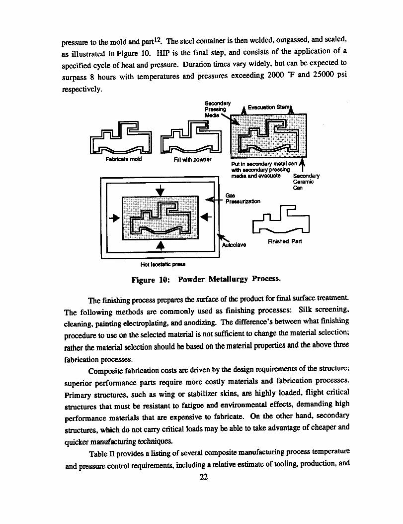
pressureto the mold and part 12. The steel container is then welded, outgassed, and sealed,
as illustrated in Figure 10. HIP is the final step, and consists of the application of a
specified cycle of heat and pressure. Duration times vary widely, but can be expected to
surpass 8 hours with temperatures and pressures exceeding 2000 "F and 25000 psi
respectively.
Figure 10: Powder Metallurgy Process.
The finishing process prepares the surface of the product for f'mal surface trealment.
The following methods are commonly used as finishing processes: Silk screening,
cleaning, painting electroplating, and anodizing. The difference's between what finishing
procedure to use on the selected material is not sufficient to change the material selection;
rather the material selection should be based on the material properties and the above three
fabrication processes.
Composite fabrication costs are driven by the design requirements of the structure;
superior performance parts require more costly materials and fabrication processes.
Primary structures, such as wing or stabilizer skins, are highly loaded, flight critical
structures that must be resistant to fatigue and environmental effects, demanding high
performance materials that are expensive to fabricate. On the other hand, secondary
structures, which do not carry critical loads may be able to take advantage of cheaper and
quicker manufacturing techniques.
Table 11provides a listing of several composite manufacturing process temperature
and pressure control requirements, including a relative estimate of tooling, production, and
22

material cost 12. Autoclave curing, which is the most versatile, has comparatively higher
tooling and production costs than the other processes. These high costs are associated with
the high temperatures (600 *F) the tools and autoclave must endure. Regardless of this,
autoclave curing is extensively used for its ability to easily manufacture a large range of
components.
Table H. Process Manufacturing Requirements and Costs 12
Process Ivtmmial Mm.erialCost
Autoclave Ola_ Kevlar,I_dlite De_/t_n °tlCuring fslic; tl_mc_As,
en mt_ choices""
Mold_ fibers; themmo_ts,
rlmsump_ _ Ke_tr ""
wm
mllibra; 0mmoOmlcsGUms,gmpU_, Xevarfibers; hisiorically withtlmmo_m; thennoplagi_
Close oole T_. Post Clue Tooll_l Production
C/wrol
Yes Yes May be requwed Low Low
Yes Yes No Low Low
Yes Yes No Depmdes on Lowpro.
Yel Yes No _" Low
Yes Yes No
No Yes No Low Low
No No Some Low Lowapt_ca_m
As well as the material mechanical properties, the size and shape of the desired part
also places constraints on the fabrication technique. Table HI presents the limitations of
certain fabrication techniques to various component forms 12. For example, large integral
structures such as fuselage skins with stiffeners, wing sections with stiffeners, and
bulkheads, can be manufactured using autoclave curing or f'flament winding. Autoclaves
are expensive with the cost being proportional to the size; a single autoclave 20 feet by 50
feet can cost $7,000,000 (for use with thermosets) or $11,000,000 (for use with
thermoplastics) 12.
Currently complex operations requiring great dexterity are manual procedures, but
some operations, such as ply cutting and lay-up are beginning to be automated, providing
substantial savings in both cost and time. These automated systems are new, and it is
difficult to predict what problems will arise.
23

Table HI. Suitability of Manufacturing Processes
to Alternative Manufacturing Forms 12
Form of Manufactured ComponentPnxess La_ Hig_y Med_arge Oosed Open Ve¢_
Integral Contorted Plain Sections Sections PartsStructure Parts Panels
Autoclave curingElastic resexv_irmolding tERM)Tnermoformingthermoplastics
Injectionmolding
Hot stamping
Rapid onethermosetsPultrusionHlamentwinding
Yes Yes Yes Yes Yes YesNo No Yes No Yes Possible
No No Yes No Yes No
No No No Yes Yes Yes
No No Yes No Yes SimpleBrackets
No No Yes Yes Yes SimpleBrackets
No No No No Yes NoYes Yes No Yes No No
2.1.2.3 Formation of the Interrelationship Digraph and the N 2 Diagram
After the key product and process characteristics are determined, the relationships
between them are identified through a prioritization matrix to define the QFD matrix roof.
The prioritization matrix was also used to identify the direction of each relationship. By
using a prioritization matrix that relates the key product and process characteristics to each
other, a correlation between each characteristic can be assigned. Through the use of a
weighting factor, a relationship can be categorized as strong, medium, or weak. From
these correlations, an interrelationship digraph is constructed that is, generally, very
muddled and difficult to understand. This digraph, as depicted in Figure 11, consists of
modules containing each product and process characteristic. Arrows are drawn to show
how one characteristic relates to another. From this interrelationship digraph, very little can
be deduced. Therefore, a tool is needed to identify in what order these characteristics can
be evaluated. DeMAID (Design Manager's Aid for Intelligent Decomposition 13) is such a
tool that provides the ability to form an NxN diagram with the above characteristics. This
program helps in planning, scheduling, and organizing the decomposition of a complex
design problem to identify its hierarchical structure.
24

Figure 11: Interrelationship Digraph of the Key Product and ProcessCharacteristics
DeMAID organizes system coupling data based on a knowledge base and displays
the results in an NxN matrix format. It takes complex data into a set of ordered,
hierarchical tasks, functions, and subsystems or modules, depending upon the level of
analysis. DeMAID actually takes the information from the interrelationship digraph and
translates it into a circuit of feed forward and feedback loops. Ideally, a minimum number
of feedbacks is desired. Also, ff smaller circuits can be modeled inside the main circuit,
then the modules in the smaller circuits can be executed by themselves after they receive
output from previous modules. Iteration processes can be accomplished on these mini-
circuits until convergence is met. From this NxN diagram, a process order is determined.
In addition, processes can also be identified that are performed in parallel with each other.
The DeMAID output using the team chosen product and process characteristics identified
for a HSCT is displayed in Figure 12.
25

MAT = MaterialsFAT = Fatigue / Sixuctm-al LifeL/D = W'm8 (L/D>MACH = Cruise lynch #GEAR -- Land/rig GearLOAD = Loads EnvelopeCORR = Corros/a_ Res]stn_eFUEL = Canve_lional Fuel
= R_ / C,ro_ We_htDIST = TIO & Landing E)/staoncesMAW = Mission Adaptive WingSPC= Low SPCEMIS = Emim'c_ Omtro]VCE = Variable Cyde Enginessum, =F.nsi_er,_e ._ss_PROP = Pr__ ulsion C..o_trolSTAB = Stal_ty Au_nentationDECK = Flight Deck
i
IS'[
_] DE,
Figure 12: NxN Diagram for Key Product and Process Characteristics
J
2.1.2.3 QFD - Product Planning Matrix
With the help of these management and planning tools, the various requirements
and characteristics were identified, a relationship matrix was constructed, and a QFD matrix
was produced. Figure 13 illustrates this Product Planning Matrix, which relates the
customer requirements to the key product and process characteristics. The arrows on the
top of the HOWs indicate the direction of improvement for each functional requirement.
The goal is to optimize, maximize, or minimize each requirement. For example, the cruise
Mach number must be optimized for a HSCT.
26

DIRECTIONOFIMPROVEMENT 0 ] ÷ I 4" I I 0 I e I0 I 0 I ÷ I I • I 0 I 0 I 0 I i I I 0 I I + I ÷KEY PRODUCT & PROCESSES
i °
iiAIRLINES
TARGETS
LOWTOC s A A 0 A A ® 0 0 A A A 0 0HIGH ROI 5 0 A 0 0 0 0 0 A /X /_ A
PAYLOAD 4 0 /_ /_. /_ _) (_) 0 /_- 0 /_-
LIFESPAN 4 0 _) 0 /k /X 0 0
EXHAUST EMISSIONS 5 /X ! /X O /X • /X O
T/O NOISE & SONIC BOOM 5 O (_) /_ O e e O /X
RECYC LABILFrY 2 O /k
FAR PRESENT k FUTURE 5 /k O A O O O
b,IRPORT REGS/ ATC 4 /% O O O _) /_i O
LOW FARES 4 /% _) O _ O /X /X /X /X /X
COUFORT _ 0 ® 0 I_RELIABLE SCHEDULE 3 /X /_ /X ./X 0 _)
ENVIRONMENTALISTS
ABSOLUTE IMPORTANCE
RELATIVE IMPORTANCE
GOVERNMENT
PASSENGERS
• ROOF MATRIX WEIGHTS
Strong Pol _ Strong (_) g
Politive 0 Medium O 3
Negotive X Weok /% 1
Strong Neg _(
lARROWS _
Mowimize
Minimize
Nominol 0
Figure 13: QFD Matrix Relating the Key Product and ProcessCharacteristics to the Customer Requirements
27

2.1.2.4 Results of Product Planning Matrix
Referring to Figure 13, one can see that, for instance, strong relationships exist
among the total operating cost and the fuel used. Take-off noise and sonic boom concerns
strongly relate to the use of variable cycle engines. Any parameter which relates strongly to
several other parameters is referred to as a driving factor. Therefore, the cruise Mach
number and engine noise suppressers were identified as the driving HOWs. The relative
importance ratings were instrumental in identifying the driving HOWs. The driving
WHATs include such items as the payload, sonic boom, and takeoff noise.
In order to examine the type of relationship each HOW has with the others, a
prioritization matrix was constructed, which can be seen in Figure 14. Notice how cruise
Mach number, high lift to drag wing, and advanced flight deck have strong or medium
relationships with many of the other HOWs. Appendix A contains explanations for each of
the strong and medium entries in the matrix. The relationships identified by this matrix
were translated into the roof of the QFD matrix. Only the strong and medium relationships
were considered for the roof. Notice that some medium relationships translated as strongly
positive or negative, and some strong relationships translated as only moderately positive
or negative. The target values were determined by researching current Literature on the
HSCT project.
_OVANCE0MATER_J.S X @ @ E) O _ ® 0 _. A ASTRUCTURAL Ltlr£/ FATIGUe"
LOAD £NV£L.oPr
CORROSION RESIS?ANCF"
L.ANO;NG GF..AR ,,
_IGH L.,/O WING
CRUIS[ MACH I
!RANG£ dk GROSS W_'IGHT
r/o & LAND DISTA_C£
20_I'/[_/T(ONAL Furl
LOW SP£CIF'SC FUk"L COMSUMP. '
CONTROt.LJ[D IrMMISSIONS
!IrNGIN£ NOIS r" SU'PPR_SORS
VARIA,BL£ CYCLE: I[NGINI"
,_Ov,_wC£0 IruGH1 ' DECX:
Is"r_t,.rtY AUaU£N'TATt0N S4tS.
,,_r_ coNTRo,..s I_SS_0N a,0J_rtvI[ WIN(;S
ADV. PROPUL$10N CONTROL
5£RW'J_gAB_LfrY
® x O®AL_@O x @®® x A!
z_i®lz_ x ®°"1, ®*/x ® 0 t®® Z_!®,
0®_
Z_ A:0 ¢xZ_
A
O_O_
A 0 [AI A 0
A 0 Ot_,1o oo_
@0 A
A0
®A®Io _® x ® 0:®A® x®0 x ®O® @IxAAA®_00A0®00A!®Z_ 0 000®A®A:®00 ®Z_0 Z_I
0 0/x
A I 0
o °o°'A 01® Z_0: ® ® A 0:
A!Z_0 Z_ 0AIO0 0 ® 0® ,,x /', IZ_0 ® 0 @x 0A 0 /x
x OZ_ 00O0 x Z_ ®Z_Z_
A,A x x@ ®i0 0 ® Z_®1® ® .® ® x 0 /"I
I0 0 x 0 iO0 i0® 0 I xz_ /,_® r® o; x:@
A ® A!,,_ 0 ® x
Figure 14: Prioritization Matrix Showing the Influence of the KeyProduct and Process Characteristics on Each Other
28

2.1.3 Establishing Value Objectives
Once the QFD matrix that relates the customer requirements to the key product and
process characteristics is formulated, the emphasis shifts to the selection of a functional
criterion. The initial system functional criterion chosen was the Return on Investment for
the airlines and the manufacturers. The next generation supersonic transport needs to be a
technological success, but even more important, it has to be economically viable. The
Concorde, for instance, has been a technological achievement, but an economic failure
never becoming capable of offering affordable ticket fares for those who want to fly
supersonically.
---
Figure 15: Return on Investment Criteria
Whether the airlines will update their future fleet with the proposed HSCT depends
on their expected ROI. The main drivers of ROI are revenue, total cost, productivity, and
utilization. The airlines' main source of income is through ticket sales. Total cost to the
airlines include fuel cost, acquisition and crew training, and life-cycle cost including
maintenance and depreciation. In addition to total cost and revenue, two other important
29/

ROI drivers are productivity and utilization. Productivity relies solely on physical factors
of the aircraft: payload, block speed, fuel, and empty weight. Utilization, on the other
hand, is given by mean time between failure, maintenance man hour per flight hour, mean
time to repair, and of course, turn-around time. A tree diagram identifying the ROI criteria
was constructed and presented in Figure 15.
The same tasks as seen before in the development of the Product Planning Matrix
were performed in the creation of an ROI QFD matrix. Once the ROI criteria have been
established, another prioritization matrix was formed in order to identify the strong
interrelationships between the ROI criteria. An interrelationship digraph that illustrates
these relationships has been generated and presented in Figure 16.
Resale Value Depreciation
a_l AcquisitionCost
Turn AroundTime
Ticket Price
Cost
Mean Time
Between Failure
Mean Time
Passenger Service n Marflaottr/
Payload Hour
Block Speed
Fuel Cost
Fuel Weight
Empty WeightCost
Figure 16: Interrelationship Digraph of the ROI Criteria
The next step in the process was to form the ROI QFD matrix. This matrix,
displayed in Figure 17, is used to determine the criteria function of a HSCT. This QFD
was used to identify all important aspects from an economics point of view.
30

DIRECTION OF IMPROVEMENT O IC) 1 41L I _1" I _j" I _Ir I _lr I C) I t I _1_ I _1, I _1, J _1_ I _I" I _j" I _1,tl i
Return On Investmenti
(HOWs) _ = _ "-_
-r-
Structures
Aerodynamics &Performance
Propulsion
Controls & Flight Systems
Ufe Cycle Cost
TARGETS
Structural Life/Fotlgue 7 j O _) II(E) /_ /_ 0 ® ® /_ 0HighL/OW_ng 9 A A 0 0 A ® A ®Cruise Moch # 9 ® /_ 0 ® 0 (_) ® /_ 0
Range & Cross Weight 8 i/_ A 0 /_ /_ 0 (_) (_) (_) ® /_
T/O &: Landing Distance 6 /_ /_ 0 C) O 0 /_
Conventional Fuel 6 ® /_ ® /_ /_ /X 0 /X /X
Lo. SFC 7 !0 A A A ® A 0Controlled Emissions 7 /_ 0 /_ 0 /_ /_ /_ /_
Eng. No[me Supp. 7 _ 0 0 /_ /_ /_ /_ /'_
Engine Choice 7 ® 0,0 /_ /X 0 _ 0 /X. /X_ /X
Mission Adop. Wings 5 /_I/_ /_ '/_ /_ 0 0 /_ 0 /_
Maintainability, 7 /_ /_ ® ® 0 /_
ABSOLUTE IMPORTANCE
RELATIVE IMPORTANCE
f ROOF I MATRIX
Strong Pos _) IStrong _)
!Positive 0 JMed[um 0
Negative X JWeak /%,
Strong Neg )_< 1
WEIGHTS
g
3
1ARROWS ]
Maximize ,_
M[nimlze
Nominal 0
= -
,_,_{__ _ _ ,i_ m = _ ,_ _. _:
Figure 17: QFD Matrix Relating the ROI Criteria to theKey Product and Process Characteristics
31/

2.1.3.1 Feasibility Constraints
The feasibility criteria are the economic, physical, performance, and environmental
constraints which must be met in order for a design to be considered a feasible alternative.
The important constraints with regards to a HSCT are shown below:
Restriction
• Controlled Emissions • < 5 gm NOx/Kg Fuel• T/O & Landing Noise * FAR 36/Stage 111• Overland Noise • < 70 dB
• Gross Weight • < 750,000 lbs• T/O & Landing Distance • <= 11.000 ft• Cruise Mach Number • 2.0 - 2.6
• Range • > 5000 nm• Structural Life • > 60,000 hrs
2.1.3.2 Life Cycle Cost Matrix
The life cycle cost of a system is defined as the total cost to the customer comprised of
acquisition and ownership of that system over its full life. It includes the cost of
development, acquisition, operation, support, and disposal as seen in the equation below:
t=rt
LCC = E (RDT& E) + (PROD) + (O&S)+ (DISP), where n is in years 14.t=0
Approximately 60% of the life cycle cost is found in the Operations and Support area. If a
company spends more on research and development to improve the reliability and
maintenance access of the aircraft, a decrease will occur in the Operations and Support area.
Minimizing life cycle cost requires the company to spend money and time up front in the
conceptual and early design stages as seen in Figure 18. On the other hand, it is important
not to lock in all of the project's finances early in the research and development stages.
Decisions made in the early design stage affect the amount of LCC to be spent later in the
life cycle of the aircraft.
A third QFD matrix was subsequently formulated and was dedicated to LCC where
the return on investment for the airlines and manufacturing (see Table IV) were related to
the cost drivers (see Figure 19). As one might notice, the ROI criteria are slightly modified
from the ROI criteria as seen in the previous QFD matrix. This is due to the fact that more
information is known about the product at this stage in a HSCT design than was known
early in the design. Also, the major reason that the ROI criteria has been changed is to
choose the ROI criteria that relates to the analysis program that was chosen to be used.
32
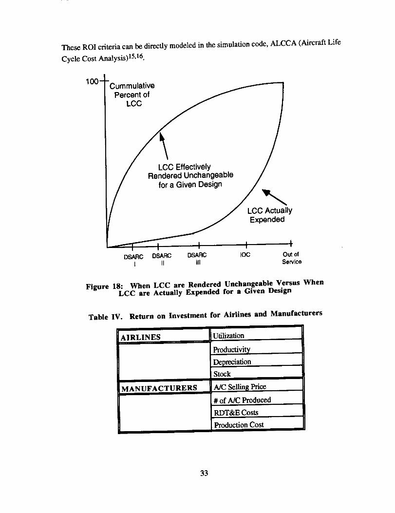
TheseROI criteria can be directly modeled in the simulation code, ALCCA (Aircraft Life
Cycle Cost Analysis) 15,16.
Cummulative
Percent ofLCC
LCC EffectivelyRendered Unchangeable
for a Given Design
LCC ActuallyExpended
I I IDSARC DSARC DSARC IOC Out of
I II III Service
Figure 18: When LCC are Rendered Unchangeable Versus WhenLCC are Actually Expended for a Given Design
Table IV.
i i
AIRLINESi
Return on Investment for Airlines and Manufacturers
!
MANUFACTURERS
Utilization
Productivity
Depreciation
Stock
A/C Sellin_Price
# of A/C Produced
RDT&E Costs
Production Cost
33

The factors which make up the ROI and the cost drivers were determined through
brainstorming. These factors were entered into a QFD matrix, and their relationships and
interrelationships were determined.
o
Airlines
Ulilizal ion
"ticket Fore
Productivity
Depreciotion
Stock
s OG O00 GG
4 G GAOA®
4 go G G O
2 O A AO
2 O O /X /X O
,_ 0 GA0S6/_ 00042
G 0 0 42IAAAAA O 60A 0 O2_
= Designers ond=, MonufocturersetJ
A/C Sell'i'ng Price 5 /X G O
# Of A/C Produced 4
R,D,T. & E
Pr oduc_.ion Cosl
0 G O G O OG G G G O_gG O0A 0 G O ®A4_
5 A G A O O (9 G G G G O O G 774 G ® A!A A A 0 0 (9 G 46
, _ "z , _
v _.. o-; z -- _
i:4i:i:& _:' e._ ._ P-- _r, -- ._ -- r---
• ,+ -.,:::::::::.; _ II_ II_ I_ Ik_ g'_ I_ I_ _ _
ARROWS }
Moximize ,ill,
Minimize _
N0mtn01 O
TARGETS
ABSOLtJ:TE IMPOR,rANCE
RELATIVE IMPORTANCE
I ROOF
trong Pos G
osltive O
egolive ×
trong Neg)_
MA'I'RIX WEIGHTS
Strong ® g
Medium O 3
Weok )'_ 1
Figure 19: The QFD Matrix Relating the ROI to the Cost Drivers
34

2.1.3.3 Average Yield per Revenue PassengerMile ($/RPM)
A metric that relates the concerns of both the airline and the manufacturer was
needed to integrate the ROI desires of both parties. This selected metric is the average yield
per Revenue Passenger Mile ($/RPM), an Overall Evaluation Criterion (OEC) that captures
the concerns of all interested parties, manufacturers, airlines, and passengers 1.
In studying the economics of a HSCT, the ticket fare for a long range subsonic
transport similar in size to the Boeing 747-400 is being used for comparison purposes.
Since the chosen metric is the average yield per RPM, the target value for this study is
based on 747-400 values of approximately $0.10/RPM. In order for a HSCT to be
economically viable, economic analysts are forecasting that the target average yield for a
HSCT should be between $0.10 - $0.13 per RPM. This claim is supported by several
market surveys which show that most passengers are willing to pay a premium up to thirty
percent more than a subsonic ticket fare 17.
2.1.4 Generation of Feasible Alternatives
2.1.4.1 Baseline Configuration
As was mentioned previously, the thrust of the effort described in this report was to
set up an IPPD method to standardize and facilitate the concept evaluation process through
MDO and Taguchi methods. Having established an understanding of the problem and
defined value objectives in the form of $/RPM, the Georgia Tech team conducted a
conceptual design study and obtained two candidate baseline configurations (a double-delta
wing concept sized with today's technology (low risk), and one for development in the
year 2005 (medium risk)). These two configurations were sized for an all supersonic
mission, depicted in Figure 20. Figure 21 illustrates the double delta configuration which
was used in this paper as a sample case for the implementation of the methodology
developed. The information for these two baselines is presented in Table V.
35

Cruite M-- 2.4
Max. Altitude
.70,000 ft
Climb
De_en d
Taxi
Land
t_ 5,000 n In v !
Figure 20: Baseline Mission Profile
Figure 21: Georgia Tech's HSCT Double-Delta Baseline Configuration
36
Table V. Baseline Configuration Descriptions
• Payload• Range• Block Fuel
• Empty Weight• TOGW
• Wing Area• Span• Taper Ratio• t/c
• Thrust/Eng.• Fuselage I.• Block Time• P.I.
1994 (Low Risk) 2005 (Med. Risk)
300 passengers, 62,700 lbs5_000 nm
423_380 lbs I 317r000 lbs344r760 lbs ] 285t000 lbs878.000 lbs I 730.000 lbs
8,500 sq. ft I 8,500 sq. ft
140 ft i 140 ft
O.O7 O.08
0.03 0.0368_000 lbs 50tO00 lbs
310 ft
4.a4 t_rs. I 4._ hrs.
92 knots [ 119 knots
2.1.4.2 Stability and Control of the Baseline Configuration
This section of the report addresses the issue of static longitudinal and directional
stability of the baseline HSCT. The main tool used was a computer program called APAS,
an acronym for Aerodynamic Preliminary Analysis System 18. APAS was developed by
Rockwell International for NASA Langley and is widely used throughout industry. Its
purpose is to predict vehicle aerodynamics at the conceptual and preliminary design levels.
The program can also determine static longitudinal and lateral stability characteristics,
which is of interest here. In analyzing the stability of the baseline, the placement of the
nacelles was varied along with the relative location of the wing with respect to the fuselage.
To show how this was done, however, some more discussion of APAS is in order.
APAS is a program that uses a panel method to generate aerodynamic forces and
moments for a given configuration. The user can create the configuration either graphically
or using ASCII fries called card files, which define the geometry. For simplicity, in this
study the geometry was defined graphically. APAS requires that the user provide the
dimensions, areas, aspect ratios, taper ratios, type of airfoil, etc. of a particular component.
The code will create that particular component as it was specified. The geometry that the
code creates is generic, so one may need to edit it so that the component is as close as
possible to the actual geometry. Editing is done manually similar to editing a CAD
drawing. A representation of a HSCT geometry is illustrated in Figure 22. Looking at the
geometry, it is easily seen that the fuselage is a perfect cylinder, and a closer inspection will
reveal that the wing and fuselage do not blend together nicely. Investigation into the
blending issue showed that the program results are not affected by an ill-blended
37
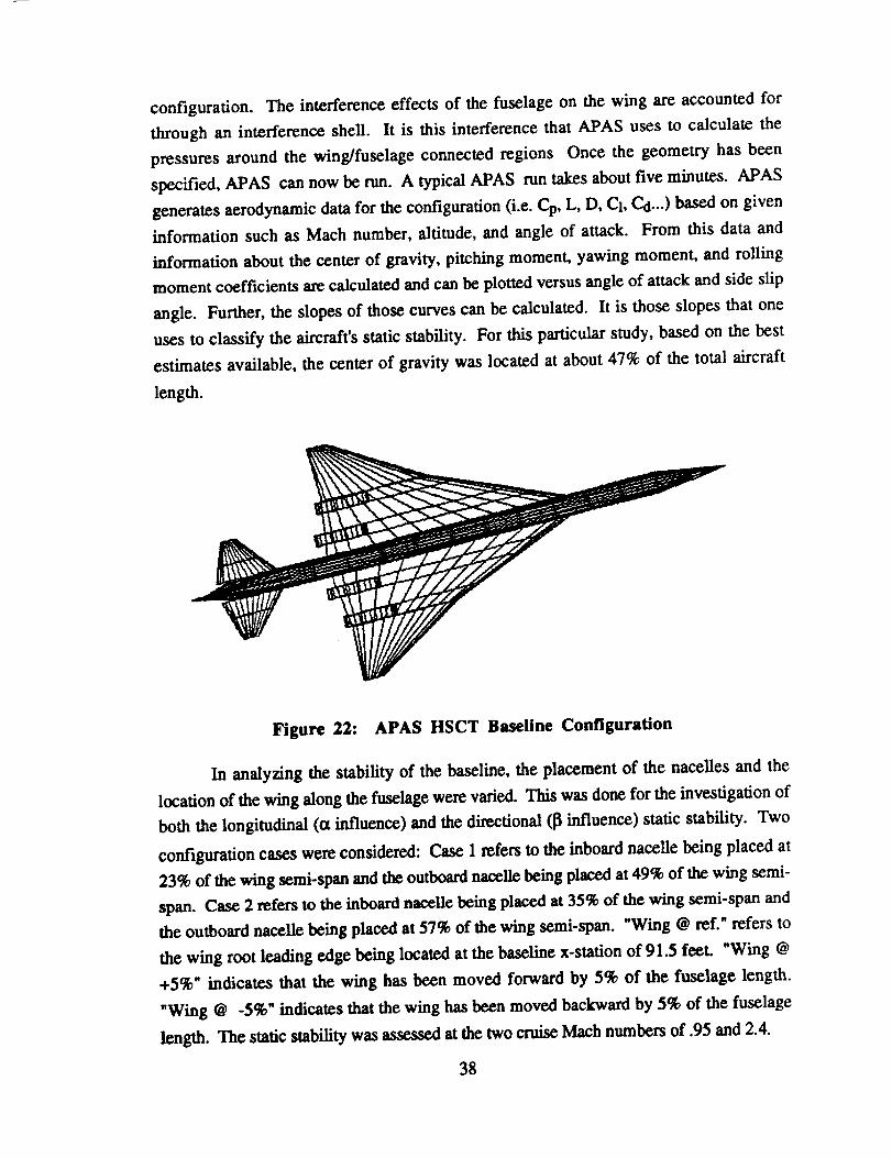
configuration. The interference effects of the fuselage on the wing are accounted for
through an interference shell. It is this interference that APAS uses to calculate the
pressures around the wing/fuselage connected regions Once the geometry has been
specified, APAS can now be run. A typical APAS run takes about five minutes. APAS
generates aerodynamic data for the configuration (i.e. Cp, L, D, Cl, C.d...) based on given
information such as Mach number, altitude, and angle of attack. From this data and
information about the center of gravity, pitching moment, yawing moment, and rolling
moment coefficients are calculated and can be plotted versus angle of attack and side slip
angle. Further, the slopes of those curves can be calculated. It is those slopes that one
uses to classify the aircraft's static stability. For this particular study, based on the best
estimates available, the center of gravity was located at about 47% of the total aircraft
length.
Figure 22: APAS HSCT Baseline Configuration
In analyzing the stability of the baseline, the placement of the nacelles and the
location of the wing along the fuselage were varied. This was done for the investigation of
both the longitudinal (a influence) and the directional (_ influence) static stability. Two
configuration cases were considered: Case 1 refers to the inboard nacelle being placed at
23% of the wing semi-spanand theoutboard nacellebeing placedat49% of thewing semi-
span. Case 2 referstothe inboard nacellebeing placedat35% of the wing semi-span and
the outboard nacellebeing placedat57% of the wing semi-span. "Wing @ ref."refersto
the wing rootleadingedge being locatedatthe baselinex-stationof 91.5 feel "Wing @
+5%" indicatesthatthe wing has been moved forward by 5% of the fuselage length.
"Wing @ -5%" indicatesthatthe wing has been moved backward by 5% of the fuselage
length.The staticstabilitywas assessedatthetwo cruiseMach numbers of .95 and 2.4.
38

Figures 23-28 contain the results of the longitudinal stability analysis. From the
plots one can see that for each nacelle - wing placement combination, and at both Math
numbers, all of the "Cm versus oc" curves have negative slopes. Thus, it can be concluded
that for each nacelle - wing combination, the airplane is longitudinally statically stable. The
magnitudes of the slopes reflect how stable each configuration is. Figure 25 shows that the
aircraft appears to be more stable at subsonic cruise speeds and gets less stable when the
wing is perturbed in either direction from the reference. Also, the aircraft is more stable
with the nacelles placed closer to the fuselage.
0,2 • , , , , • •
0.I
t -0.1
-0.2
-0.3
-0.4
i i i
! i i i _,i ! i
. . . i . . . t . . , [ ..... .[ , , , i , , . i • • . i , • •
-4 -2 0 2 4 6 8 10 12
IX
Figure 23: Case 1 - CmVs. cx @ Maeh = 0.95
39

0.1 '''1''' '']I''" '_'1'''1"*'
i
.................@.................................. _..................._...................,...................|..................._.................0.05 : ! : : _, _ ;
i i I-o-win8 e_f I................._-.-_ .........i...................i..................j--_wm_ @ +5% | .............
° 1"%-o,os .................i ' "T'""_-_..................; .................._ _ ..........i......................................i..................4.................! ! ! _i i i
_.1 ................._------------------_.----.---..---..-__.i............................i..................._.................
-0,I5 .................:..................:..................]...................:......................K'--:...................:.................o,.................::::::.................-0.25 ......................................................................................................... ---_-..-.--.-_.---_ ................
-0.3 , , , _ , , , i .............. i , , ,
-4 -2 0 2 4 6 8 10 12
Figure 24: Case 1 - Cm Vs. ot @ Mach = 2.4
-0.022
-0.024
-0.026
-0.028t5tl
-0.03
-0.032
-0.034
' I ' ,
J'---_ c_ 1:wing e r,f. I
...................."]+ Case I: Wing @ +5% I ...................................................../¢....[--. o--.Case 1: Wing @ -5%
/
/
i /!........................................................................i......................z:...........:...............................
i i / ii i /
...................................i....................................................
i /: _ i
0.5 1 1.5 2 2.5
Msch Number
Figure 25: Case 1 - Cma Vs. Mach = 2.4 & 0.95
4O

l!
O.l
-0.1
-0,2
-0.3
-0.4
iI_wi,,__,,,. i
..................................i_iiiiiiiiiiiiiiiiii_iiiiiiiiiii_'i"..................i...................;.................._............................... ,i-...................;.................................
, , , 1 , , , , , , , a ......... I , , , I , , ,
-4 -2 0 2 4 6 $ I0 12
Figure 26: Case 2 . Cm Vs. ¢x @ Mach = 0.95
0,1
0.05
-0.05
-0.1
-0.15
-0.2
-0.25
' ' • r • ' ' ' , , • , ! , , • " , • • • • ,
.................i..............-..................i..................-..................i..................T..................i.................
.................i..................i-_i .................._................i-'-_, _+_i............i i..................................i i i _i i ! i
' ..............."..................:.'-..................i...................+--,,<-.........!..................i ..................i.................i i i i .',,i i i
.................i.................._..................i..................i ...................._ ........."..................i.................i i i i >.i i i i i _ !
................-,':..................:'-..................i..................-..................i..................._-..........................i i i i \_i i i i i i i
-4 -2 0 2 4 6 8 10 12
Ct
Figure 27: Case 2 - Cm Vs. cx @ Mach = 2.4
41

-0.024
-0.026
-0.028
-0.03
-0.032
-0.034
0.5
Figure 28:
--o--Case 2: Wing @ ref.
+ Case 2: Wing @ +5%
.... o-- Case 2: Wing @-5%
/
/
Figures 29-32 show the result for directional yaw stability. From the plots of the
"Cn versus 13", the requirement for static directional stability (or weathercock stability) is
that the slope of the "Cn versus _" curve be positive. Figs. 30 and 32 show that this
configuration has neutral directional stability at Mach 2.4 (i.e. cruise). This is usually
acceptable, especially since large directional damping is not needed at such speeds.
Looking at the Mach .95 plots, it is seen that nonlinear results are obtained. This is due to
the fact that APAS has modeling difficulties at transonic speeds. The slopes, however, are
still always positive so the airplane is laterally stable, though results at transonic speeds are
often suspect. It can be concluded that since Cnl_ is positive for all nacelle wing
combinations, these configurations are at best slightly stable directionally, but more
probably neutrally stable, especially at cruise. Since the magnitudes of the slopes are so
small it can also be concluded that the airplane has poor damping in yaw. In other words,
for a small disturbance, the airplane is very slow to recover.
42
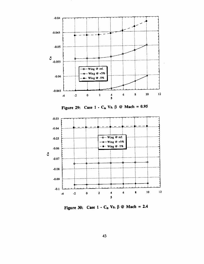
II
-0.04
-0.045
-0.05
-0.055
-0.06
-0.065
........ I " " " ' " " I ...... I " ' '
............... ......... ..................................
................ "-.................. t- ................. t .................. t .................. t ................. t. ................. _ ................
I I
--e--wing @ rcf. i
| + W'ing @ t-5_ i
...... i _. _---,--_'_... i . _ i . _ i , . ,
-4 -2 0 2 4 6 8 10 12
Figure 29: Case 1 . Cn Vs.[3 @ Math = 0.95
-0.03 .................... , . ,
Ig
-0.04
-0.05
-0.06
-0.07
-0.08
-0.09
-0.1
|
................. z.................. !.................. I ""_"'" Wing @ ref. ........... ,.................. ,.................
i i I] ..._.._ Wing @ +5%
................. i.................. _i.................. "_---.'- Wing @-5% ............ ,....................................
................._..................._.................._..................$.................._.................._.................._.................i i i i
. . , t . , , i , , , t , , . n , , , j , , , ] , , _ t . , .
-2 0 2 4 6 8 lO 12
Figure 30: Case 1 - Cn Vs. _ @ Math = 2.4
43

-0.015
-0.02
-0.025
-0.03
-0.035 ....................
-0.04
• ' , I , ' • I • • • I • ' • t ' • ' I , , • ! ' ' • ! , . ,
i _ i i i*................4.................._..................i..................;.............................._-./_--................................
E
................_................._..................!..................!..................i..................iy/¢ ................i i i i _
..................... ;............ _.,................ ¢......................................
---o---Wing @ ref. [
---a--Wing @ +5% I
i i, , , I , • , I , , . t . , , I , . , I , • • I , , . i , , .
-4 -2 0 2 4 6 8 10 12
Figure 31: Case 2 - Cn Vs. _ @ Mach = 0.95
0.01 ............. I ...... _ " ' •
• ......... e" .......... ,b.......... • ......... 9 .......... "e ......... •0 ................ _ ................. • ................... "..................................................... - ..................................
| , ........................
-o.ol ................7................._..................i.................71-o- wing_ l_f.
i i ! il-+-'Winge +5_-0.02 ................-_................._..................i................._[---.e--Wing @ -5% ........................
-0.03 ..............._ v_ _; v.k .,.'_- _ v................
-0.04 .............................................................................................................................................
-0.05
...*., .9.. ,9,..*...9,, ,_., ,9..,
-2 0 2 4 6 8 I0
P
12
Figure 32: Case 2- CnVs.[_ @ Mach = 2.4
The lateral roll stability results, "CI versus [Y', are shown in figures 33-36. The
requirement for lateral stability is that the slope of the "C1 versus [3" curve be negative.
Therefore, Figures 34 and 36 show that the airplane is almost neutrally stable at Mach 2.4.
44

At the Mach .95 cruise condition, nonlinear results are again obtained. As mentioned
before this is due to the transonic speed of Mach .95. The slopes, however, are still
negative; therefore, for these configurations, the airplane appears to be laterally stable. The
slopes for these curves were calculated along the most linear portion of the curve and were
found to be about -.000058, indicating again that the damping in roll is very weak. Again,
since the magnitudes of the slopes are so small for all cases, it can also be concluded that
the airplane has poor damping in roll. In other words, for a small disturbance, the airplane
is very slow to recover.
-0.4702
-0.4703
-0.4704
-0.4705
-0.4706
CI =-.000058B
-2 0 2 4 6 8 10
Figure 33: Case 1 - CI Vs. _ @ Mach = 0.95
12
45

-0.411 • ' ' , ' • ' I ' • ' i • ' ' I .... ' , ......[ _ ! !
................_ .................:.................:................._..................4................._ .................;................
-0.412 }
.... _ ......6 ; --*-..... 6 ---_-0.413 .......................................................................................'....................................................
iiiiiiiiiiiiilI-0.414 --o--Wing @ ref. '.............................................................................
---e--Wing @ +5% CI _.000046
--o-- Wing @ -5% I_-0.4]5 ...........................................-..................................
-0.416 ................_- ................ 4b="'=-===ll:-:="::::_ i""""'"''_"'"'"'"'"_i ..............
04, i i,.t ii.-4 -2 0 2 4 6 8 I0 12
B
Figure 34: Case 1 - C!Vs.[_ @ Mach : 2.4
-0.4844
-0.4845
-0.4846
-0.4847
-0.4848
-0.4849
CI _.000056
-4 -2 0 2 4 6 8 I0
Figure 35: Case 2. CI Vs. [_ @ Mach = 0.95
12
46
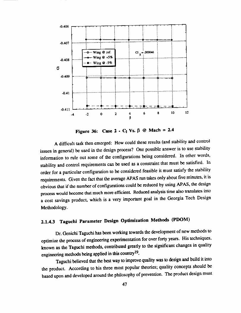
-0.406
-0.407
-0.408
-0.409
-0.41
-0.411 ' "
-4
................_.................:........................................... _ ..............._ ................_ ...............
----o----.Wlng @ ref. CI 1_=-.000046
...........l_Wing @ +5% .................,..................,.................._..................,:.................
["'"'" Wing @-5% iT
._----_-----+..___,.._____..____
• ?-. .-,'P",; ;-"I'-,- ,9-,-..--*-.- .=--*--.-:-.--o...
-2 0 2 4 6 8 10 12
Figure 36: Case 2 - CI Vs. [3 @ Mach = 2.4
A difficult task then emerged: How could these results (and stability and control
issues in general) be used in the design process? One possible answer is to use stability
information to rule out some of the configurations being considered. In other words,
stability and control requirements can be used as a constraint that must be satisfied. In
order for a particular configuration to be considered feasible it must satisfy the stability
requirements. Given the fact that the average APAS run takes only about five minutes, it is
obvious that if the number of configurations could be reduced by using APAS, the design
process would become that much more efficient. Reduced analysis time also translates into
a cost savings product, which is a very important goal in the Georgia Tech Design
Methodology.
2.1.4.3 Taguchi Parameter Design Optimization Methods (PDOM)
Dr. Genichi Taguchi has been working towards the development of new methods to
optimize the process of engineering experimentation for over forty years. His techniques,
known as the Taguchi methods, contributed greatly to the significant changes in quality
engineering methods being applied in this country 19.
Taguchi believed that the best way to improve quality was to design and build it into
the product. According to his three most popular theories; quality concepts should be
based upon and developed around the philosophy of prevention. The product design must
47

besorobustthat it is immuneto theinfluenceof uncontrolledenvironmentalfactors. His
secondconceptdealswith actualmethodsof affectingquality. Hecontendedthatquality is
directlyrelatedto deviationof adesignparameterfrom thetargetvalue,not to conformance
to somefixed specifications.Finally, histhirdconceptcallsfor measuringdeviationsfromagivendesignparameterin termsof theoveralllife cyclecostsof theproduct19.
The Taguchi method,as appliedto aircraft designat GeorgiaTech during theaerospace systems design process, is summarized in Figure 37 and is one way to optimize
a chosen criterion. This technique plays a vital role in Georgia Tech's CE methodology in
addressing the robustness of the design alternatives (see Fig. 3). The advantages of using
Taguchi methods include:
• Increased efficiency of the simulation process• Brings robustness into the design• Simplification of simulation models• Determination of "optimal" regions and reduction of the design space for
optimization• Incorporation of Risk analysis in the design process• Generation of sensitivities of the factors
Reference
Lectures
AE 8113Notes
Brainstorming
HOW's
Cost Drivers
WHAT'sROI
FLOPSm
Baseline
HSCT
Drivers Noise Factors ]Control Factors
Figure 37:
Level 1
la'agu ' Level2
HSCT Economic Sensitivity Assessment Methodology
The Taguchi method implements a partial factorial design of experiment instead of a
full factorial experiment to reduce the costs associated with numerous tests or simulations.
The conditions for each factor in the partial factorial experiment are determined by a set of
48

orthogonal arrays (OA). An OA or "balanced" array is defined as a standardized, balanced
table used to determine the influence that each of the control factors have on the Overall
Evaluation Criterion (OEC) using the least number of experiments 19. These OAs are then
used to lay out the design of experiments. Since the emphasis of this study is to provide a
way to investigate feasible alternatives in the most cost effective manner, great benefits can
be achieved by the incorporation of Taguchi's techniques.
Taguchi's PDOM implementation is comprised of the followi _,_ :._cps (see Figure
38):
* Identification of the Quality Characteristics and Design Parameters throughbrainstorming
. Design of Experiment(s)o Selection of suitable simulation method(s). Simulation Results Interpretation• Determination of "Optimal" Conditions• Confirmation of the "Optimal" Conditions
°
DO LOTS OF
THINKING
(BRAINSTORMING)
PLAN EVERYTHING
TO BE DONE
2.
.
4.
5.
DESIGN EXPERIMENTS
I
Figure 38: The T_chl Method Flow Chart
In order to design an experiment, it is necessary to select the most suitable
orthogonal array, assign the factors to the appropriate columns, and describe the trial
conditions. Through a series of brainstorming sessions, the various, relevant design
49
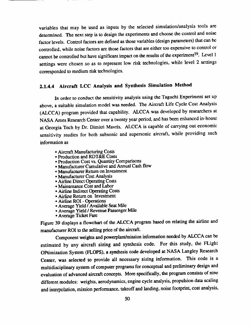
variables that may be used as inputs by the selected simulation/analysis tools are
determined. The next step is to design the experiments and choose the control and noise
factor levels. Control factors are defined as those variables (design parameters) that can be
controlled, while noise factors are those factors that are either too expensive to control or
cannot be controlled but have significant impact on the results of the experiment 19. Level 1
settings were chosen so as to represent low risk technologies, while level 2 settings
corresponded to medium risk technologies.
2.1.4.4 Aircraft LCC Analysis and Synthesis Simulation Method
In order to conduct the sensitivity analysis using the Taguchi Experiment set up
above, a suitable simulation model was needed. The Aircraft Life Cycle Cost Analysis
(ALCCA) program provided that capability. ALCCA was developed by researchers at
NASA Ames Research Center over a twenty year period, and has been enhanced in-house
at Georgia Tech by Dr. Dimitri Mavris. ALCCA is capable of carrying out economic
sensitivity studies for both subsonic and supersonic aircraft, while providing such
information as
• Aircraft Manufacturing Costs• Production and RDT&E Costs
• Production Cost vs. Quantity Comparisons• Manufacturer Cumulative and Annual Cash flow• Manufacturer Return on Investment
• Manufacturer Cost Analysis• Airline Direct Operating Costs• Maintenance Cost and Labor
• Airline Indirect Operating Costs• Airline Return on Investment
• Airline ROI - Operations• Average Yield / Available Seat Mile• Average Yield / Revenue Passenger Mile• Average Ticket Fare
Figure 39 displays a flowchart of the ALCCA program based on relating the airline and
manufacturer ROI to the selling price of the aircraft.
Component weights and powerplant/mission information needed by ALCCA can be
estimated by any aircraft sizing and synthesis code. For this study, the FLight
OPtimization System (FLOPS), a synthesis code developed at NASA Langley Research
Center, was selected to provide all necessary sizing information. This code is a
multidisciplinary system of computer programs for conceptual and preliminary design and
evaluation of advanced aircraft concepts. More specifically, the program consists of nine
different modules: weights, aerodynamics, engine cycle analysis, propulsion data scaling
and interpolation, mission performance, takeoff and landing, noise footprinL cost analysis,
50

andprogram control. Although FLOPS already has a built in economic analysis capability,
developed by Dr. Vicki Johnson, it is only suitable for subsonic aircraft. Therefore,
ALCCA was selected for the study as a more suitable cost analysis method for supersonic
aircraft.
E'NO_T'I¢IqlUS'r& WQHT.
PIqOOUCTIONQUANIll"Y
LEARNINg
AIRCRAFTMANUFACTURING
COSTS
LABOR• IIUADI_
PRICE
CALCULATE
NO
TOTAl.OPERAT_
Figure 39: ALCCA
AIRLINERETURN ON
INVESTMENT
Flowchart
2.1.4.5 Test of Economic Analysis on the Baseline I
Before embarking on the preliminary design methodology, a test case was run in
order to determine if the LCC analysis program would be suitable for this experiment. A
list of control and noise factors were selected to model the experiment. Four of the chosen
factors were found to affect directly the various component weights and, in general, the
aircraft size; Math #, Range, Payload, % composites. Therefore, before ALg2CA could be
run, FLOPS had to be called upon four times to account for these variations. The total
weight of the aircraft varies depending upon which level is chosen for the design range.
Using FLOPS to calculate the individual component weights, the percent of advanced
technology light-weight composite materials in ALCCA was also taken into account to
determine their effect on the I.,CC of the system. AI._CA uses five different variables to
identify the percent of composite material to be used: zero percent indicates conventional
51

materials while one hundred percent denotes the maximum use of composites. The values
input into ALCCA for the two composite material levels were zero percent and sixty
percent. The values for the different component weights were computed with and without
composites at a range of 5,000 nmi. and 6,500 nmi. Once these values are obtained from
FLOPS, they were then inserted into the ALCCA program to perform the necessary life
cycle cost analysis for a HSCT.
Since in this case, the analysis was carried out from an airline's point of view, the
ROI for the manufacturer was used as a noise factor, while the ROI for an airline was
considered to be a factor that airlines can control or select. The ROI for the airline was
allowed to vary between eight and twelve percent, while the levels for the manufacturer's
ROI were chosen to be between ten and fourteen percent. Since there were concerns
associated with the feasibility of a low cost, supersonic transport, the values for the ROI
ranges were conservatively selected. At these levels, a corresponding average yield / RPM
was calculated in order to achieve the specific ROIs for the airline and manufacturer.
Table VI. Economic Sensitivity Analysis Ground Rules and Assumptions
HSCT Production scheduled for the year 2000Estimates are in 1994 U.S. dollars
i| =
Performance
Weights/InteriorCrew
Cruising altitude at 70,000 ft.100% learning curve for propulsionFour engines / aircraft
Three person crewCoach Passengers / Flight Attendant is 38First Class Passengers / Flight Attendant is 11Airfine revenue is based on a load factor of 65%Aircraft corr_nent weights are estimated from a synthesis code
Spares 6% of total airframe price30% of total engine price
Rates
Burden
Financing
Depreciation
Labor rate of $19.50 / IxTax rate of 34%Inflation rate of 8%
200% of labor
100% @ 10.25% interest rate0% down payment
Hull insuranoe is 0.35% of aircraft cost
15 years; 10% residual
Several assumptions had to be made in order to run the ALCCA program, and a list
of the most significant ground rules/assumptions is presented in Table VI. As far as the
use of composites is concerned, although composites are in general lighter in weight, they
axe usually more expensive. Figure 40 summarizes complexity factors for various52

conventionalandadvancedmaterials.For this study, a $55flb graphite epoxy material was
used that has complexity factor of 1.03 or 3% more than aluminum. In addition to this list,
another simplifying assumption was made regarding the component weights. These
component weights change in actuality not with respect to the percent composites used and
the flight range, but also vary with respect to changes in the design cruise Mach number. If
more precise results were to be obtained, then FLOPS could be run an additional four times
for the different Mach numbers, and new component weights would need to be calculated
before performing the cost analysis on the aircraft. ALCCA was modified in order to treat
the ROI for the airline as an input. A corresponding average yield increment was also
included in the program to create tables based on certain yield per RPM (i.e. $0.10 -
$0.13/RPM). This approach is aimed at comparing the average yield per RPM for a HSCT
to the average yield / RPM for aircraft similar in size to the Boeing 747-400.
(1.30) I_l Lsbor rl Material
.(!._15). _ o .o5) 0 .o=1
i ...............
if: .ii11111"i":::ii/i
aALUMINUM ALUMILITH TITANIUM KEVLAR GFIPIEPX
SSSllb.
MATERIAL
(l.,t)
:::::::::::::::::::::::::::
i:!i:?!::i::i: " 7:::i
?_xxxxxx_x
GRPIEPX
SeOIIb.
Figure 40: Complexity Factors
The finalized list of control and noise factors with respect to ALCCA are displayed
in Table VII and VIII, respectively. As mentioned previously, these factors were identified
with the help of the LCC QFD matrix. These variables were subsequently used to define
an orthogonal array. An LI6 matrix was used to represent the control factors in the inner
array, while an I.,4 was used for the noise factors in the outer array (Table IX).
53

Table VII. Control Factors as They Relate to the ALCCA Program
Factors
Cruise Mach #
Engine Cost
% CompositesROI Airline
Payload
ALCCAVariables
CMACH
CTJIPWBODY
RTRTNA
WPAYL
Utilization UMTIR ERR
I.earning Curve LEARNTurn Around GRNDTMTmae
Range SL
Level 1
2.0
$60 Million0%
4%
58,800 lbs.
280 passengers4,000 hrs.
5,000 hrs.90%2 hrs.
Level 2
2.6
$40 Million60%
12%
67200 lbs.
320 passen[ers6,000 hrs.15,000 hrs.
75%
0.75 hrs.
5,000 nmi. 6,500 nmi.
Table Vlll. Noise Factors as They Relate to the ALCCA Program
Factors
Fuel Cost
Manufacturer'sROI
Production Rate
ALCCA
Variables
COFLRTRTN
NV
Level 1
;0.17 / lb.
10%
400
Level 2
;0.09 / lb.
14%
700
2.1.4.5.1 Simulation Interpretation
Once the sixty-four (16 x 4 trials) simulation runs are completed, the results are
extracted from ALCCA and are placed in the corresponding "simulation results" columns of
the complete OA. Next, the influence of each factor on the quality characteristic is
determined by evaluating the main effects and their influence in a qualitative way. Then,
through an ANalysis Of VAriance (ANOVA) technique 19, the relative influence of the
individual factors is identified to provide a measure of confidence in the Taguchi Method
results. The Signal to Noise (S/N) ratio for each case is calculated to examine the
variability associated with the multiple trial results. The S/N ratio is the variance index that
is determined by the results obtained by repetition. Regardless of the type of quality
characteristic selected, the transformations are such that the S/N ratio is always interpreted
the same way: the larger the S/N ratio the better. The greater the Signal to Noise ratio, the
smaller the variance around the target value. The Signal to Noise ratio is based on the mean
square deviation (MSD) from the target value of the quality measure (i.e. yield/RPM). The
MSD can be calculated several ways depending on the quality characteristic that is
chosen 19. For example if the quality characteristic is smaller is better, the MSD is
calculated as follows:
54

_D_.(yI2+y2 2+...)
n
where yis are the results of the experiments, and n is the number of repetitions. The S/N
ratio can then be computed as follows:
S / N = -10 Iog,.(MSD)
The three quality characteristics available for determining the optimal condition are:
• "smaller is better"• "nominal is best"
• "bigger is better"
For a HSCT, the overall evaluation criterion selected was the average yield / RPM;
therefore, smaller is better. The analysis will therefore answer the following questions:
• "What is the optimum condition?"• "Which factors contribute to the results and by how much?"
• "What will be the expected results at the optimum condition? ''16
2.1.4.5.2 The Experiment
In the first part of the project, ten control factors, one interaction between factors,
and three noise factors were identified. The objective of this experiment was to find the
control factor levels (see Table VII) that would be the least influenced by changes in the
noise factors (see Table VIII), and would result in the "best" combination for the airline
return on investment. Since this was the fh-st time the experiment was attempted, no a
priori knowledge was available as to which factors are the most important ones, and thus
all of them were given equal importance and kept for further study. The control factors
were tested using two levels instead of three in order to minimize the number of
experiments and avoid the difficulty of creating interactions between three levels. The
approach presented here is best suited for determining the effect that each of the control
variables has on the evaluation criterion. It is therefore used for sensitivity analyses rather
than the selection of an "optimum" configuration. Since the true optimum result will most
likely lie somewhere between the two levels selected, the experiment can be repeated (once
the number of control factors is reduced through this analysis) with more levels producing
a real optimum. The noise factors were also varied between two levels.
55

Table IX. The Complete Orthogonal Array for the Design of Experiments
i
OOL
00_
eleEl
uo_npoJd
i
f,|
Otu
IOEI=unloelnuel/_
Zl.'0
|too len-I
t
°
sut.unloo
le^e'lt le^e7
;,-,- o o ...... ; ,- ,- ,- ;
n"
Oel_'Z
gZ'O
g/."0
Lg0000'0Y
.
09'0
ggL'g
00'_
06"0
_X)O'O
V/N
(%) eu!p!VIO1:1ellsOdUJOO%
t I.x 8 uo!lome|ul
09'_ 00"_
i_le_'l t le_'l
|$o0eul_)u3pee_S _q8
i
Jolo_.-I
03
O4
0
O_
O0
U_
Oe
56

The OA selection was based on existing arrays found in Ref. 19. This selection
process is significant in setting up the design of experiments. An L16 inner orthogonal
array was selected for the control factors, since an L12 is not suitable for the analysis of
interactions. The L16 orthogonal array calls for sixteen simulation runs to be conducted,
which by definition is a set of trials equivalent to conducting 215 = 32,768 possible
combinations that yield an indication of the "optimum" combination. Notice in Table IX
that there is an interaction between Utilization and MTI'R, which was placed in Column
three.
The three selected noise factors were placed in the 1.4 outer orthogonal array. The
ones and twos in the inner and outer matrices represent the levels at which those factors
should be set during the experiment These two arrays have been combined in the manner
shown in Table IX to form the complete design of experiments layout. The layout also
includes a data matrix where the experiments ($/RPM) are recorded.
The four observations recorded for each simulation trial condition capture the effect
that the noise factors have on the overall evaluation criterion. Once these probability
distributions due to noise are computed, in addition to the mean responses, the combination
of control factors that give the optimal result (while achieving robustness) was determined
by performing an ANOVA on the results presented in Table IX.
2.1.4.5.3 Result Interpretation
In order to automate the evaluation process, a software package, Qualitek-4
(QT4) 20, developed by NUTEK, Inc. was used. Once the quality characteristic was
decided (average yield / RPM) and the results were obtained from ALCCA, the next step
was to evaluate the S/N ratio based on the MSD. The main effects of the S/N ratio on the
control and noise factors were computed with the help of QT4, and an Analysis of Variance
Analysis (ANOVA) was subsequently performed using this information to determine the
optimal condition for the quality characteristic of "smaller the better", as well as their
relative contributions. Since no a priori knowledge existed on the feasibility of a
$0.10/RPM, a 20% increase was assumed to be a reasonable guess. Therefore, a target
value of $0.12 dollars per RPM was used. Figure 41 illustrates the result distribution
obtained by running the sixty-four experiments.
After the analysis was carded out, the control factor level combinations that yield
the optimal configuration were obtained (see Table X). The control factors not listed in this
chart were found to have a very small effect on the measure of quality, and were thus
"pooled" together. The findings presented in Table X are best illustrated in Figure 42,
where the relative importance of each factor is shown quantitatively. For example, the
57

manufacturer'slearningcurve was found to have the largest effect on the total system,
which means that any improvements that can be made on reducing first unit cost (lean
aircraft initiative) or simply lowering the learning curve for a given production lot will
reduce significantly the aircraft acquisition cost, and consequently, the average yield per
RPM. On the other hand, if a factor like the Mean Time To or Between Repairs (MTI'R) is
varied, a minimal variation of the overall evaluation criterion will he observed.
15.25 8.45
Figure 41:
°
8.66 15.06 1.87 1.27 1.40 1.68 l.OO 2.89 2.29
Average Yield / Revenue I'lt_senger Mile ($ / 10)
$/RPM Variations for All Experiments PerformedIncluding the "Optimum" Distribution
Table X. The Optimal Configuration for the "Smallerthe Better" Quality Characteristic Case
ControlFactors
Cruise Mach#
Engine Cost% CompositesROI Airline
i
Pa_.loadUulization
Mean Time to
RepairLearning Curve
Range
Level
22
1
2
2
2
2
1
Description
M=2.6 atcruise
40M dollars
60 %
8%
67200 lbs.
6000 hours
1/15,000hrs
75%
5,000 naut.miles
%Influence
7.25 %
2.1)5 %3.59 %
3.89 %
16.01%
15.57 %
0.46 %
34.53 %
15.19 %
58

Learning Curve
Engine Coat
_ite
ROI Airline
Block Speed
Payload
Figure 42: Control Factor Influences on Average Yield / RevenuePassenger Mile ($/RPM)
For the optimal condition, the analysis selected an airline ROI value of 8% and a
payload of 67,200 lbs, which corresponds to a passenger count of 320. The learning curve
level was assigned to be 75%, while the range was set at its lower value of 5,000 nautical
miles.
The average signal to noise ratio was calculated to be 16.7157 for this "smaller the
better" case. Using this ratio, the optimal configuration listed in Table X was obtained.
The "minimum" expected average yield / RPM was found to be $0.104/RPM, which
corresponds to an aircraft acquisition price of $227.85M (see Figure 43 for "best" and
"worst" distributions) and an average ticket fare of $606.788 (Figure 44). This $/RPM
result corresponds to just a four percent increase over the minimum assumed yield for the
equivalent subsonic transports, and it corresponds to an expected improvement of 17.39%
with respect to the worst case scenario depicted in Figure 44.
In order to understand the influence that the various control factors have on the
evaluation criterion, the levels were allowed to vary from the best level to the worst, one at
a time. The results from this exercise are presented in Table XI. As can be seen from this
table, the average yields are higher than the optimum, but within the acceptable range
(compared to existing long range subsonic transport ticket fares) for most of the cases
examined. For example, if the manufacturer's learning curve was allowed to vary from its
optimal level of 75% to its highest allowable value of 90% (see Table XI), the overall
evaluation criteria will vary from $0.104/RPM to $0.12/RPM. This example indicates how
59

variation with respect to a given control factor affects the optimal condition as it is
determined by PDOMs. Since the noise factors can not be controlled, there are no set
levels for these factors; thus, a variation from the target value will always occur. It is due
to these noise effects that Figures 41, and 43-45 show variation rather than singular values.
The interaction between M'ITR and Utilization that was incorporated into the inner
array turned out to have a minimal effect and was pooled together with other small values.
When transferring the factors into QT4, this interaction was thought to be significant.
However, it turned out to be very weak due to the fact that the sizing program (FLOPS)
and ALCCA did not take into account this relationship.
Optimum
8.67 1.21 1.75 2.29 2.84 3.38 3.92 4.47 5.ei 5.55 6.18
Aircraft Acquisition Price (Millions $ x 100)
Figure 43: Aircraft Acquisition Price Variationfor the "Optimum" and "Worst" Conditions
Optimum
8.29 8.48 8.51 8.62 8.73 8.84 8.95 1.86 1.17 1.29
Average Ticket Price ($ x I000)
Figure 44: Average Ticket Price Variation for the"Optimum" and "Worst" Conditions
6O
1.48

Optimum _.
[__8.25 8.58 8.75 1.81 1.26 1.52 1.77 2.83 2.28 2.54 2.79
Average Yield / Revenue l'w_enger Mile ($ / 10)
Figure 45: $fRPM Variation for the "Optimum" and "Worst" Conditions
Table XL Change in Average Yield per RPM from the "Optimum"Condition
Control Factors
Learnin/_ Curve
Utilization
Range
Block SpeedROI Airline
% Composites
Levels
2_1
2tol
2tol
lto2
2tol1102
2Iol
$/RPM
0.120
0.115
0.115
0.114
0.111
0.109
0.109
2.1.4.5.4 Confirmation Test
The finalstepof the Taguchi PDOM isto run a testto conf'u'mthe "optimum"
condition.Using the levelsobtainedforthe optimalconfigurationas determined from the
QT4 program, a conf'u'mationtestwas executed usingALCCA. The resultsobtained from
this test verified the optimum condition and are displayed for review in Table XII.
Table XII. The "Optimum" Condition Confirmation Results
NRPM
Result #1 0.1198
Result #2 0.1166
Result #3 0.0903
Result #4 0.0977
61

As previously mentioned,theaverageyield perRPM for the optimumcondition
was$0.104. Theaverageof thefour confirmationtestcasesgivesa valueof $0.106perRPM. This variationis dueto thenoisefactors,which is thereasonwhy theconfirmationrun hasfour different values. Theconfirmationtestverifiedthattheoptimal condition is
viable.
2.1.4.6 Top Level Orthogonal Array
The first step in Georgia Tech's preliminary design methodology is the actual
generation of feasible alternatives. This is done through Taguchi's PDOM. A top-level
decision orthogonal array was defined with feasible configurations characterized by the
type of engine (MFTF or TBE), cruise Mach number (2.2, 2.4, or 2.6), the type of
mission (all supersonic or split subsonic/supersonic), the number of passengers (300 or
320), and the wing type (conventional or advanced technology, i.e., hybrid laminar flow
control). The top-level feasible alternative OA can be seen in Table XIII.
Table XIII. Top-Level Decision OA
Level 1
2.4
Wing Type
Level 2
2.0
Engine Type TBE MFTF
Mission All Supersonic 25% Subsonic
# Passengers 300 320
Conventional HLFC
2.1.5 Evaluation of Alternatives
The decomposition and recomposition process for each of the feasible
configurations presented in Table XIII can be best illustrated by Figure 46. The
methodology developed is based on breaking down the various tasks of interest into their
corresponding product and process characteristics, and all relevant design and
manufacturing variables that should be considered were identified. The problem was then
decomposed down to the individual disciplines where the optimization tradeoffs between
the product and process design parameters take place at the component level. Once the
"optimal" configuration is chosen at the component level, the information is passed back to
the system level where tradeoffs take place with respect to the overall evaluation criterion
selected for the system.
62

DECOMPOSITION
Feasible Configurations [
Product Process
Aerodynamics\ Structures] Propulsion Manufacturing
RECOMP0SITI0N
Discipline I Part Level
Discipline Experts
t/c, k, A, \ # Spars and I TIT, OPR, Tooling,
Ribs. ] etc...Geometry,\ SelectionMaterial etc...Tolerances,
Component Level - Component Optimization
Designert,(L/D)c _ Ww/ft2, SFC, _- Manuf.(L/D)to, Xetc... \
Trades - Overall Evaluation Criteria
Systems Level - Systems
Performance & Economics
P.I. Manuf.Cost
ROI airlineROI manufacturer
Overall Measure ofQuality of the HCST
$/RPM
Make Derisions ]
Customer
Figure 46: Feasible Alternative Evaluation Flowchart
A robust design assessment was conducted for each of these cases at the component
level leading to the selection of a set of "optimal" wing/nacelle configurations. These
63

combinations were selected for a combined aerodynamic/structures and manufacturing
point of view. Figure 47 illustrates this optimization procedure flow. Once the "optimum"
wing geometry and characteristics are defined, the problem is recomposed back to the
system level where the synthesis/economic analysis are performed, and the "optimum"
overall configuration is chosen from an economics point of view. (Average Yield / Revenue
Passenger Mile).
AERODYNAMICS
STRUCTURES& MATERIALS
___ WING [CONFIG.
,LMANUFACTURING METHOD
L.Ww
D
OECis - OECs for the various win S configuratlons ],analyzed at different methods of manufacturing. I
-MTT-(FULL FACTORIAL EXPERIMENT)
Figure 47: Wing Optimization Procedure
2.1.5.1 Aerodynamics Orthogonal Array
The following wing planform definition, displayed in Figure 48, was introduced to
geometrically define both double delta and arrow wing configurations. From an
aerodynamic design point of view, the performance criterion that best describes the quality
of a design is the Lift to Drag ratio. In order to maximize this ratio, the "optimal" design
variable settings must be determined. First, a list of key design variables for an integrated
nacelle/wing configuration was composed. The control variables selected define the wing
geometry, airfoil shapes, and fuselage attitude. The factors that the aerodynamicist does
not have absolute control over were considered to be noise factors. The noise factors
selected included the wing location, nacelle location, and nacelle size. These factors
64

accountfor the effects that handling qualities, aeroelasticity, structures, and propulsion
sizing will have on the cruise L/D. Fifteen control factor variables were considered for
further study. In order to reduce the size of the combined aero-structures experiment, the
relative importance and influence of each of these variables was identified through a
separate aerodynamics experiment (this aerodynamic study was carded out using the
Boeing Design and Analysis Program (BDAp)21). Therefore, a preliminary Taguchi
experiment was conducted to identify the factors that contribute/affect L/D the most in the
chosen range of values. The control and noise variables selected for this experiment are
presented in Table XIV and XV, while the relative control factor influences are illustrated in
Figure 49. The results presented in Fig. 49 were obtained through an ANOVA by
optimizing the Signal to Noise (S/N) ratio. The five most important design variables were:
the longitudinal wing leading and trailing edge "kink" locations ( X1 and X2 normalized by
the chord root coordinate), the root t/c, maximum thickness location at the root, and the
fuselage angle of attack. The average I./D ratio and corresponding standard deviation after
the optimization turned out to be 8.62 and 0.30 respectively, while the average L/D ratio
and corresponding standard deviation before the optimization were 8.02 and 0.30
respectively.
(x2,Y2) (x3,Y2)
Ct
)
Cr
Figure 48: Wing Pianform Configuration
65

Table XIV. Aerodynamic Experiment Control Factors
Factors
X1
X2
X3
](4v1
Y2
Y3
(t/c)r
(t/c)tMax_ Thick. @ Root
Level
0.667ii
O.qlq1.0
0.q_6
0.4890.259
2.9
2.0
Level 2
0.767
1.001.10
1.0o
0.4390.209
2.7
1.5
50% 60%
50% 60%Max. Thick. @ Tipnacelle height -5 -7
Dist. btwn nacelles 14 1_Fuselage aoa 3 " 6 "
Win_ Hei_,ht 0% -50%
Table XV. Aerodynamic Experiment Noise Factors
Factors
Scaling factor of Nacelle
Rel. Long. Loc. of
wing wrt fuse.
Nacelle Placement
Level 1
1.0
0.289
0.364
|
Level 2
1.2
0.239
0.464
These most significant contributors were next used in the combined Aerodynamics-
Structures-Materials OA experiment, while the rest of the aerodynamic design variables
were held at the levels that yield the "optimum" L/D.
66
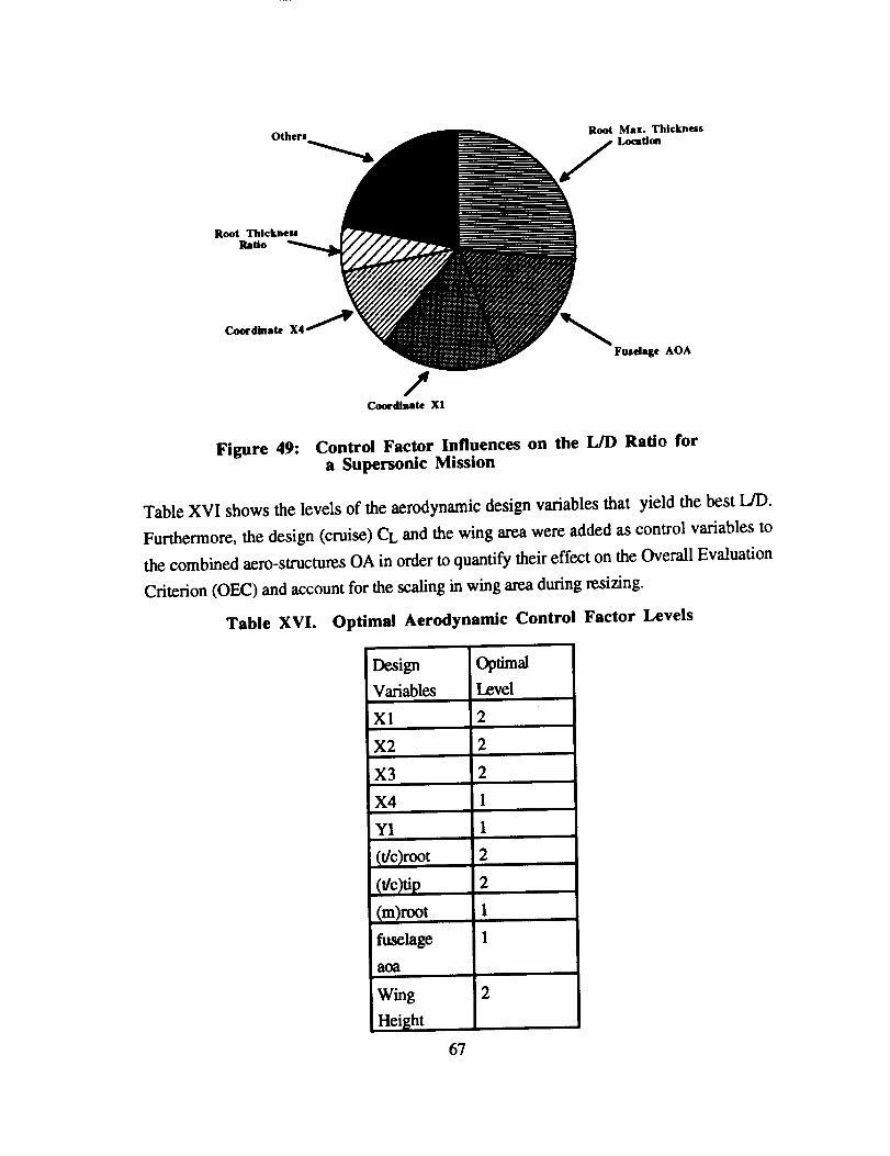
Root Max. ThicknessLocation
Coordinate
/Coordlms_e XI
F_el_e AOA
Figure 49: Control Factor Influences on the L/D Ratio fora Supersonic Mission
Table XVI shows the levels of the aerodynamic design variables that yield the best L/D.
Furthermore, the design (cruise) CL and the wing area were added as control variables to
the combined aero-structures OA in order to quantify their effect on the Overall Evaluation
Criterion (OEC) and account for the scaling in wing area during resizing.
Table XVl. Optimal Aerodynamic Control Factor Levels
Design
Variables
Xl
Optimal
Level
2
X2 2
X3 2i i
X4 1
Y1
(t/c)root
(m)root
fuselage
aoa
Wing
Height
Ii
2
2
67

2.1.5.2 Aerodynamics, Structures, and Manufacturing Opt. Wing
Since the focus of the methodology implementation task was the design and
optimization of a Nacelle-Wing configuration, an OEC function that captures the
aerodynamic, structural, and manufacturing design aspects was selected. This chosen OEC
(for the wing component) is presented below as:
OEC i = Ix
L-Ww ]D .+
Ww Nlrwbase.]
where L and D in this equation represent the wing Lift and Drag, Ww denotes the wing
weight, and Nrw corresponds to the manufacturing cost.
Finally, ot and 1_are weighting factors selected by the team members to represent
the relative importance of cost with respect to the performance criterion chosen. Since the
two contributing factors (product and process side) have different units, the two quantifies
were normalized by their corresponding baseline values. The $/RPM still remained the
overall system criterion function.
2.1.5.2.1 Combined Array: Response-model/combined-array approach toNacelle-Wing-Fuselage Integration
Assessing robustness through the use of the outer array concept increases the
number of experiments significantly since the noise array has to be repeated for every row
in the control array. Due to large computer run times associated with finite element
methods (ASTROS), it became evident that a further reduction in the number of
experiments conducted was necessary.
It has been proposed earlier that to generate an "optimum" Nacelle-Wing
configuration, the aerodynamic, structural, and manufacturing design aspects need to be
integrated together in the preliminary design stage. However, the integration of
considerations from different disciplines is usually not an easy task. One of the many
reasons is that more computational efforts would be involved during both design analysis
and synthesis processes for an integrated design. It was introduced before that Taguchi's
quality engineering method can be used to increase the efficiency of the simulation process,
bring robustness into the design and generate the sensitivities of the factors, etc. Although
the methods have been widely used, there is still much room for improvement. In this
section, the response-model/combined array approach, a modification to the Taguchi
method is applied to the integrated Nacelle-Wing-Fuselage design. The limitations of the
68
Taguchi method, the two part experimentation strategy, and the loss-model approach are
presented in the proceeding sections. In addition to these limitations, the literature of
response-model/combined array approach, some of the benefits of using this approach, and
the procedure of implementing this combined aerodynamic, structures and manufacturing
experiments are also provided.
2.1.5.2.2 Limitations of Taguchi Method
Taguchi provides a method supported by statistical techniques and metrics to assist
engineers in establishing and improving a product's quality. His principles have been
widely used to design quality into products and processes (Ref. 22-25). However, this
method has also received criticisms from the American statistics community (Ref. 26-28).
The major argument is that the statistical techniques proposed by Taguchi are not
theoretically based or efficient enough and there is still room for improvement. Alternative
experimental formats, design criteria, analysis techniques, graphical tools and optimization
strategies therefore have been proposed by the American statistics community to overcome
the difficulties.
Relevant to the application of Taguchi method in this work, i.e., the robust design
optimization by simulating design models, the limitations of Taguchi method can be
classified into two categories. The first category is related to Taguchi's two-part
experimentation strategy, and the second one is associated with using the signal-to-noise-
ratio as the performance criterion, sometimes called loss-model approach. Further
explanation is provided as follows:
2.1.5.2.3 Limitations of Two-Part Experimentation Strategy
Taguchi recommends a two-part experimentation strategy to solve the robust design
problem. Using his approach, the control factors (C) are varied according to a "control
array", sometimes called inner array. For each row in the control array, the noise factors
(N) are varied according to a "noise array", called outer array. This is schematically
represented in Figure 50. There are two major limitations associated with this inner-outer
array approach:
• Very large number of runs may be required because the noise array is repeated for
every row in the control array.
• Because of the structure of using both inner and outer arrays, there is no flexibility
to use some of the degrees of freedom to estimate interactions between control factors and
noise factors (C x N). As the idea of robust design is to select the levels of control factors69

to minimize the effects of the noise factors, it is necessary to examine the C x N interactions
so that the control factors that have a dampening effect on individual noise factors can be
identified.
CONTROL ARRAY
Figure 50:
Row A B C D
I -I -1 -1 -I
2 -1 -1 1 1
3 -1 1 -1 1
4 -1 1 1 -1
5 1 -1 -1 1
6 1 -1 1 -1
7 1 1 -1 -1
8 1 1 1 1
NOISE ARRAY
Row a b
1 -1 -1
2 -1 1
3 1 -1
4 1 1
Row a b
1 -1 -1
2 -1 1
l -I
4 1 1
Two-Part Experimentation Strategy for Robust Design
2.1.5.2.4 Limitations of the Loss-Model Approach
In Taguchi's robust optimization, the objective function is to maximize the signal-
to-noise ratio. Each noise array provides an estimate of this optimization criterion,
represented by R, and new control-factor levels are identified by treating R as the
dependent variable and examining control-factor main-effect and interaction plots and
ANOVA. This approach to identifying new control-factor levels is called the loss-model
approach because it is based on modeling the loss directly as a function of the control
factors. There are several disadvantages of using this approach:
• The focus is on modeling R, which is often a nonlinear, many-to-one
transformation of the response Y. It is less likely that R can be modeled well by a low-
order linear model even if data transformations are employed.
• As the relationship between R and the control factors has not been quantified, in the
case additional quality characteristics need to be considered, it is very difficult to do the
70

tradeoffsquantitatively. In thepreliminarydesignof complexsystemslike aircraft, the
considerationsof multiplequalitycharacteristicsarealwaysnecessary.
2.1.5.2.5 The Use of Response-Model/Combined-Array Approach
To overcome the limitations of Taguchi method, a natural alternative is to model the
response Y instead of modeling loss R and use the response model to discover control-
factor values that help reduce variability. This approach is first proposed by Welch, et al.
(Ref. 29) to remedy the aforementioned disadvantages in the context of computer
experiments. The major dements of their approach are:
* combining control and noise factors in a single array,• modeling the response itself rather than expected loss, and* approximating a prediction model for loss based on the fitted-response model.
Shoemaker, et. al. (Ref. 30) further developed and strengthened this response-
model/combined-array approach. They showed that run savings from using combined
array are due to the flexibility that this formulation allows for estimation of effects.
Using the response-model/combined-array approach is effective in this project, due
to the fact that there are large computer run times associated with finite dement methods
(ASTROS). It becomes evident that reduction in the number of experiments conducted is
necessary. The computational time can be greatly saved by using the combined array
approach (Instead of 16x4 experiments by inner-outer array approach, 16 experiments is
needed using this method). Furthermore, there are several other benefits in using this
approach:
* It is very easy to identify the control factors that have a dampening effect on
individual noise factors by taking a look at the magnitude of the C x N coefficient in the
response model equation.
• Since the response model is a low order math model, with some simple
mathematical expansion, we can estimate the performance variation under different noise
factor variations without running further experiments.
* The response model represents the mathematical behavior of the wing design.
When later a HSCT design is integrated at the system design level, this equation can be
used to estimate the wing weight value, instead of calling aerodynamic and structure
analysis packages again and again.
71

2.1.5.2.6 Implementation Procedure of the Combined Array Experimentfor the Nacelle-Wing-Fuselage Integration
To apply the response-model/combined-array approach to a HSCT Nacelle-Wing-
Fuselage integration, an Overall Evaluation Criterion function that captures the
aerodynamics, structural, and manufacturing design aspects will be taken as the overall
quality characteristic to choose the "optimum" wing. The design objective in wing robust
optimization is to maximize the mean value of OEC and minimize the variation caused by
the noise factors around this mean. The eleven control factors (design parameters) are
contributed by both major aerodynamic and structure design parameters, e.g., spar/rib
number, material, coordinates, Nacelle placement, lift coefficient etc. Some of the noise
factors include engine weight, wing area, fuel weight etc. Following the response-
model/combined-array approach, we will go through the following procedure:
Step 1 Create a combined array including both control factors C and noise factorsN. In this case, L16 standard array (16 experiments) is used for testing 11control factors and 4 noise factors. The factors and their levels selected are
presented in Table XVII.
For each of the 16 experiments, steps 2-4 are repeated:
Step 2 An aerodynamic analysis (using BDAP, WINGDES, and AWAVE) isperformed to compute the corresponding L/D ratio for the wing, and the CLdistribution is used as an input to ASTROS.
An ASTROS preprocessor is run to set up the finite element model.
The ASTROS experiments are run to compute wing weights, etc.
Based on the 16 experiment results, estirnate control and noise main effects(C and N) and C x N interactions. During this process, normal distributionplots, interaction plots or other statistical analysis techniques wiU be used toidentify the significance of different factors.
The use of wing area as the response of the combined OA methodologyadopted for the aero-structures experiment enables the determination ofcoefficients for a "wing area equation"; these coefficients will yield a moreaccurate wing weight for FLOPS when the aircraft is resized for a givenmission.
For each of these aero-structures combinations, a full factorial
manufacturing experiment is conducted.
A response model is fitted which represents the relationship between theresponse, OEC, and the significant C, N and CxN factors.
Based on the equation obtained from step 8, the "optimum" control factorsare chosen, which can maximize the mean value of OEC and reduce the
variation caused by the noise factors around this mean.
Step 3
Step 4
Step 5
Step 6
Step 7
Step 8
Step 9
72

Table XVII.
#
Structure/Aerodynamic/Material/Manufacturing CombinedControl and Noise Factors
Control Factors
Svars/# ribs o/# ribs il_fafarial _lartinn
Coordinate X1
Coodinate X4
Rnnt (flc_
Coordwise Location
of Max. Thick. @ RnntNacelle Placement
Fuselage aoaTiv (t/c)
lift te"n_ffl rl _n t
Coordinate X3
Nac. Size / Ene. Wt.w
Win_ Area
Horiz. 1_. of wing
Fuel Wei_ht
Level 1
4/10
Madi.m Riglc
0.667
0.956
qo/,,
5O%
2.0
n qq
1.00
35 ft / 17,000R._f}O fta2
0.289
350,000ii
Level 2
6/8Mic, h Ri_k
0.767
1.00
60%
0.464
6"
1.5nll
1.10
42 fL /22.000
10.000
0.239
500,000
Combined AeroJStr./Materials OA
One Combined L 16U Control Factors
4 Noise fatteN: Eng wt., Wlq Area,X., Fuel wL
Step 5
[ Estimate main effects (C &N), and ]interactions (C x N)
Step 6
Fit a response ModelWeight = [_0 + Y_I3jC+ T._jN + Y_[_kCxN
q
Steps 1 - 4
I' Step 7
Manufacturin_ Cost
st,p_sFit an OEC Model I
c=p.+zp,c+zpjN+zp.c.NI)
Step 9
Choose the optimum levels of control factors 1based on Mean(OEC) and Var(OEC) [
I
Wing Weight = f (Eug wt., Wing Area,
X,,, Fuel Wt.) OEC_
Figure 51: Combined Orthogonal Array
73

The steps are depicted graphically in Figure 51. The result from step 9 yields a
robust "optimum" design for a HSCT wing. The wing weight equation, the optimum wing
and the distribution of OEC will be brought as the input information to the next design
stage.
A design of experiments was set up to determine the minimum wing weight and the
corresponding variation distribution from this optimum. For this case, the wing taper ratio,
sweep, t/c, wing area, nacelle placement, number of spars, beams, and ribs, the skin
thicknesses, etc. were allowed to vary in order to obtain this "optimum" wing.
From the first case from the uppermost orthogonal array, which is for an all
supersonic mission at Mach 2.4 using a turbine bypass engine as well as the information
contained in the aerodynamics/structures orthogonal array, sixteen cases in ASTROS were
run.
Two combinations of spars and ribs were considered in the design. The first
combination included four main spars on the aft wing, ten ribs on the outboard portion of
the wing and seven ribs along the inboard and forward section. The second spar and rib
combination uses six main spars in the inboard section of the wing, eight ribs on the outer
portion of the wing and seven ribs along the inboard and forward section.
To study the structural aspects of the design, a finite element code, ASTROS
(Automated STRuctural Optimization System31), was used. ASTROS can be used to test
the effect of different types of materials, structural concepts on wing weight, aeroelastic
behavior, flutter, and manufacturing cost. It is uniquely suited for flight applications
because performance considerations such as flutter can be addressed. ASTROS allows the
user to input an initial design and then optimize it for weight by imposing constraints. For
the cases considered in this project, the wings were analyzed at full and empty fuel
conditions for a 2.5 g pull up maneuver, making sure that all flutter and material strength
constraints were satisfied.
For each simulation run, the CL distribution corresponding to the selected wing
planform was provided to ASTROS from BDAP as well as the material(s) chosen. The
actual materials were selected by carrying out a critical point design on the wing.
According to this technique, three to four points were selected on the wing based on high
load or stress concentration. The wing was then divided into regions as seen in Figure 52
that include these critical points, and it was assumed that the same material and
manufacturing process will be used for every part in the region.
74

(1)[] (2)
• Part Design
• Nrw for each region (3)• Sum to get total Nrw for OEC
[]
Figure 52: Wing Manufacturing Consideration, Three Point Design
All wing spars and ribs were assumed to be made of the titanium-aluminum alloy
Ti-6A1-4V, while the material for the skin of the wing selected depended on the wing
section location. As mentioned previously, three sections were chosen on the wing, and
the materials were chosen for each section as shown below in Table XVIII:
Table XVIII. Material Selection
Section
Forward
Inboard
Outboard
Medium Risk
IM71520
Ti-6AI-4V
T650-35/R8320
High Risk
MR50/5208
Ti-6AI-4V
ApoHo-55-
800/KIll
ASTROS was run next to determine the corresponding wing weight for each of
simulation cases that were set up. The results of each case were analyzed, and the most
influential contributing factors were identified along with the optimum level combination
and the risk associated with the design choices made. Next, the designer's production cost
trade-off tool 32 were used to determine the cost of the wing structure, and the results of this
investigation were then incorporated along with the wing weight distribution into FLOPS
and ALCCA. The approach outlined in the previous two tasks was then repeated to obtain
the configuration that yields the minimum $/RPM.
75

The Structural analysis(ASTROS)needed information about the aerodynamic
characteristics of the wing in the form of aerodynamic load distributions. The spanwise lift
variation on the wing was provided to ASTROS from BDAP, while the chordwise el was
assumed to vary linearly.
Once again, appropriate ranges were selected for each of the selected control/noise
factors (assuming two levels, minimum and maximum), and a suitable orthogonal array
was chosen. The aerodynamic simulations were calculated using BDAP, WINGDES,
AWAVE, etc. Once the combined nacelle-wing-fuselage configuration geometry was
defined (fuselage geometry remained fixed throughout the study), BDAP was called upon
to predict the pressure distribution over the wing accounting for nacelle-wing and fuselage-
wing interactions. These pressure distributions were then integrated to yield lift and drag
due to lift. WINGDES was called to provide the optimum twist and camber distributions
for the computed lift value, while the overall wing drag was calculated based on the skin
friction and wave drag contributions computed by BDAP and AWAVE, respectively. The
most significant aerodynamic design parameters determined from the aerodynamic design
of experiments were used for the combined aero/structures experiment, and the
corresponding wing weight was calculated. The overall result of this design of
experiments was an "optimum" wing geometry ("Optimum" in a linear sense; the true
optimum exists somewhere in between the two levels selected), and a lift and drag
distribution that is used by FLOPS and ALCCA (Aircraft Life-Cycle-Cost Analysis) to
minimize gross weight and $/RPM distributions, respectively.
An ASTROS preprocessor was used to create the file for each of the sixteen cases
of the L16 using geometric, aerodynamic, and material information. Once the ASTROS
runs were obtained, a post processor was used, along with the database created by
ASTROS, to calculate the weights of the different wing components. These weights were
then given to the manufacturing members of the team to calculate the cost of manufacturing.
The information from aerodynamics, structures, and manufacturing was then used to obtain
the "optimum" wing.
2.1.5.3 Manufacturing Implementation
Once ASTROS has calculated the material thicknesses and area deformations that
satisfy the static loads, dynamic loads and flutter, Georgia Tech will use the Manufacturer's
Trade Off Tool. This is based on the following equation:
Cost = Weigh# X b + (Weight X c)/Q
Cost: Manufacturing cost in $
76
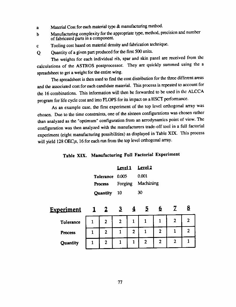
a Material Cost for each material type & manufacturing method.
b Manufacturing complexity for the appropriate type, method, precision and numberof fabricated parts in a component.
c Tooling cost based on material density and fabrication technique.
Q Quantity of a given part produced for the first 500 units.
The weights for each individual rib, spar and skin panel are received from the
calculations of the ASTROS postprocessor. They are quickly summed using the a
spreadsheet to get a weight for the entire wing.
The spreadsheet is then used to find the cost distribution for the three different areas
and the associated cost for each candidate material. This process is repeated to account for
the 16 combinations. This information will then be forwarded to be used in the ALCCA
program for life cycle cost and into FLOPS for its impact on a HSCT performance.
As an example case, the first experiment of the top level orthogonal array was
chosen. Due to the time constraints, one of the sixteen configurations was chosen rather
than analyzed as the "optimum" configuration from an aerodynamics point of view. The
configuration was then analyzed with the manufacturers trade-off tool in a full factorial
experiment (eight manufacturing possibilities) as displayed in Table XIX. This process
will yield 128 OECis, 16 for each run from the top level orthogonal array.
Table XlX. Manufacturing Full Factorial Experiment
Level 1 Level 2
Tolerance 0.005 0.001
Process Forging Machining
Q_anlity 10 30
Eroeriment 1 2 3 4 5 fi Z 8
Tolerance 1 2 2 1 1 1 2 2
Process 1 2 1 2 1 2 1 2
Quantity 1 2 1 1 2 2 2 1
77

2.1.5.4 Synthesis/Propulsion/Economic Analysis
For the propulsion downselecdon study, two engine cycles were considered, the
Mixed Flow TurboFan engine, and the Turbine Bypass Engine concept. NASA Lewis and
NASA Langley have carded out similar studies trying to optimize the SFC, NOx
emissions, noise levels, and thrust produced for these engines. This study had similar
objectives testing each engine cycle after they have been integrated on the various candidate
configurations and mission profiles. Once again, the Taguchi orthogonal array (design of
experiments) technique was used to determine the best combination of engine parameters
that yield an "optimum" $/RPM.
Table XX. Propulsion/Sizing/Economic Experiment Control Factors
Control FactorsII
Overall PR
Fan PR Ionly for MFTF)
comp. exit airflow ratio
(only for TBE)
Turb. Inlet Temp.
ROI Airline
Utilization
Turn Around Time
MTTR
Level 1
18
2
O.O7
2800 deg. R
10%
4t000 hr.
2.0 hr.
1/5,000 hr.
Level 2
4
0.10
3400 de 8. R
14%
61000 hr.
0.75 hr.
1/15,000 hr.
The experiment setup started, once again, with the identification of the key engine
design variables to be considered as well as the selection of the appropriate ranges for them
(minima and maxima). These design variables included such parameters as the bypass
ratio, the fan and compressor pressure ratios, the turbine inlet temperature, the combustion
chamber temperature, the turbine cooling flow, etc. These variables were considered as
control factors for the design of experiments. From an economic viability point of view,
the factors selected included the ROI for the airline, the aircraft utilization rate, the turn
around ground time, and the mean time between repairs. This short list was chosen based
on prior experience that the team acquired while carrying out a similar study at the
conceptual design phase. The noise factors selected included the fuel cost price, the
number of aircraft produced, and the manufacturer's learning curve. The selected list of
78

control and noisefactorsis presentedalongwith their correspondinglevels in TableXXandXXI.
Table XXI. Propulsion/Sizing/Economic Experiment Noise Factors
Factors
Fuel Cost
Production Quantity
Learning Curve
Level 1
$0.09/Ib.
400
82%
Level 2
$0.17/]b.
7OO
9O%
For these factors, the ROI for the manufacturer was set at 12%, and the engine
acquisition price was allowed to vary as a function of Mach number, thrust, and technology
factor. The engine acquisition price fell between 2.5 to 4 times greater than the engine
acquisition price for current subsonic transports.
The actual simulation results were obtained from QNEP/FLOPS (Quick NASA
Engine Program/FLight OPtimization System) and ALCCA. It was essential that the
control/noise factors selected matched those used as inputs by these programs. Qualitek-4,
a Taguchi software package, was used to perform the analysis of variance and obtain the
"optimum" results and assess the risk associated with obtaining these values. Although
QNEP/FLOPS and ALCCA are not integrated together, only one design of experiment is
necessary (using a much larger orthogonal array) with an overall evaluation criterion at the
system level given by the yield per revenue passenger mile.
Table XXII. "Optimal" Control Factor Settings
Control Factors
OPR
Comp. Ex. Airflow
Turb. Inlet Temp.
ROI airline
Utilization
Turn Around Time
Mean Time to Repair
Level
1
2
1
1
2
2
2
Description
18
0.10
2800 deg R
10%
6_00 hr.
0.75 hr.
1/5,000 hr.
% Effective
0.63%
pooled
4.69%
1S.89%
74.49%
0.16%
2.85%
79

For the first feasible alternative design combination (top array), the analysis yielded
the "optimal" control factor settings presented in Table XXII and Figure 53. These figures
also illustrate the relative importance that each control factor has on the $/RPM criterion.
Figure 54 illustrates the result distribution obtained by running the 32 cases in FLOPS and
ALCCA. For the case where all of the top level orthogonal array variables were set to level
1, the $/RPM was found to be in the order of $0.128 / RPM.
Figure 53: Significant Control Factor Influenceson the System OEC, $/RPM
8.28 8.54 8,79 1.B4 1.29 1.54 1.79 2.84 2.29 2.54 2.79
Average Yield / Revenue Passenge_ Mile ($ / 10)
Figure 54: $/RPM Variations for the First Feasible Configuration of theTop Level Orthogonal Array Including the "Optimum" Distribution
8O

2.1.6 Making a Decision
In order to design an experiment, it is necessary to select the most suitable
orthogonal array, assign the factors to the appropriate columns, and describe the trial
conditions. Through a series of brainstorming sessions, the various and relevant design
variables that may be used as inputs by the selected simulation/analysis tools are
determined. The next step is to design the experiments and choose the control and noise
factor levels. Level 1 settings are chosen so as to represent low risk technologies, while
level 2 settings correspond to medium risk technologies.
The feasible alternatives selected in step 4 of this methodology can now be
evaluated through the use of a series of Taguchi experiments. The overall evaluation
scheme is illustrated in Figure 55. Inspection of this figure indicates that all the feasible
alternatives can be placed in a top decision matrix OA. For each and every one of the
combinations identified from this array, an aerodynamics/structures and manufacturing
example simulation is conducted to determine the "optimum" wing configuration, as well as
the relative influence/importance that each of the design variables considered has on the
wing OEC.
Once the "optimum" wing is selected, information related to its geometry,
aerodynamic characteristics (CL and CD distributions, etc.), and weight (as a function of
wing area) are passed to a synthesis/sizing code (FLOPS). Propulsion related (engine
sizing) design variables are also selected to evaluate each of the feasible configurations at
the system level. FLOPS sizes the aircraft and provides all the necessary aircraft related
information to the ALCCA code, which computes the average yield per Revenue Passenger
Mile. If noise factors are considered at this point (i.e. fuel price and production quantity),
then a distribution of $/RPM is obtained, and the selection is based on obtaining a
configuration that not only yields the minimum $/RPM but which also reduces the variation
due to noise around this "optimum". Once all top level cases are calculated, an analysis of
variance is conducted to determine which overall configuration yields the optimum $/RPM.
The new "optimum" design configuration, which will be identified once all
experiments described in Figure 55 are performed, will then have to be subjected to a series
of double-check tests to verify that all constraints are satisfied (NOx, noise, takeoff length,
etc.) including a stability check. The stability and control cheek is essential since the
empennage dimensions were selected based on chosen volume coefficients that may or may
not be correct. Both the constraint and stability cheek will eventually include results
obtained at takeoff, cruise, and landing.
81

Stmttures
Codutrolfactor chosenas Jcombination of no
of spars/ribs
Mate, riskTWo combinations
_ of materials chosenj
LA) -cruise
I II 'Top ieyel OA [LS] Best $/RPM value& distri-]
Feasible alternative, s bution for each alternative. I
_ ,Aerodynamics [L-I 6]
Expet'iment to identify 5
2 factors significant factors
Outer array : L-4 ; corr.
to Slr ucturcs, Propulsionand Handling qualities
Control and Noise factors placed together
in the smae array.
Sructural design/materials
I Full factorial exp.- Manufaclnring ]T : refers to diffe_nt processes Wing weight
_ Non-recuning cost
_(OEC(i) ;ANOVA for die OECs_)_.-.---
1
J ragPolars
Geometry
Wing Weight Eq.Manufacturing Cost
[ IJl ii
_ Siring / Propul_ion (FLOPS) [ JInner array : [L-8]; ou/er [L-4] ] ]
I i I co.pied
i. Weight dislr_utions_ Productivity [ TogetherI Ind©x I
II I
I ItJ_ CY_ _ _al_ (A_EA) I iII ] ,Inner array: [D$] ; outer : [L.4]I
m ANOVA
in $/RPM: target ]J
$/RPM
Figure 55: Concept Evaluation Experimental Schematic
The implementation of this methodology and the execution of all experiments
presented for the determination of the "optimum" configuration will be the focus of next
82

year's design course sequence. The results will be presented at the annual ADP
conference.
3.0 Conclusion - Future Work
The completion of the concept evaluation phase leads to the validation of the IPPD
methodology, the shrinking of design space into 'optimal' regions, and the understanding
of significant contributors and their effects. The knowledge obtained thus far can then be
used in formal optimization schemes that have been developed for MultiDisciplinary Design
Optimization. The use of Orthogonal Arrays (Taguchi Methods and the Combined Array
method) make the extraction of sensitivities simpler. Future work shall focus on making
use of the simplified model to derive Sensitivities and consequent application of Sobieski's
Global Sensitivity Equation method and/or Response Surface Methodology. Since the
methodology is well suited for the latter method, it will probably be explored to a greater
extent.
The response-model/combined array approach has been used in this project to
improve the computational efficiency for robust design by combining control and noise
factors in a single array. Due to the scope of this project, the fitted response model only
determines the coefficient of the main factors (control factors C and noise factors N) and
the interactions between control factors and noise factors (CxN). Therefore, it is close to a
first order polynomial approximation. Plus the fact that the experiment is only designed for
2 levels of each factor, it is difficult to capture the nonlinear behavior of the system, and,
thus, the results obtained might not be an accurate one. To improve the accuracy of robust
optimum, it is suggested to use second (or higher) order polynomial approximation for the
response model in the future work. There is a formal technique called Response Surface
Methodology (RSM) to support these activities 33.
Different from the traditional regression analysis, using RSM, a series of
experiments are set up for measuring the response of interest. A model is then fitted based
on the experiments results. In order to construct a second-order surface model, each
design parameter must be analyzed at a minimum of three levels. The design for this
experiment is called central composite design. Simply speaking, the central composite
designs are the first order fractional factorial designs augmented by an additional "star" and
"center"s which allow the estimation of a second order surface. Having obtained the
response surface model, the mean and the variation of the response can be calculated, and
the "optimum" design can be achieved based on the robust design criterion.
Overall, the benefit of using RSM in this work lies in the fact that this method
allows for rapid exploration of the given parameter space and the determination of
83

sensitivities. In constrained robust optimization, it allows for easy modifications to the
constraints bounds, without having to go back to perform additional experiment. This is
very appropriate for the concept exploration of complex engineering systems such as
aircraft.
Further work is also needed in each of the disciplinary contributing analysis to
make the methodology more rigorous.
84

4.0 Appendix A
Strong Relations of the Product Planning Matrix & the Value Objectives Matrix
HOW
Structural Life / Fati_ueHigh Lift / Drag Wing
Cruise Mach Number
Cruise Mach Number
Range / Gross Weight
Controlled Emissions
Conventional Fuel
!Engine Noise Suppressers
Engine Noise SuppressersEngine Noise Suppressers
Engine Choice
Maintainability
Product Planning Matrix
WHAT
Life SpanPayload
T/O noise & Sonic Boom
Low Fares
Payload
Exhaust Emissions
Low Total Operating Cost
T/O noise & Sonic Boom
Airport Regulations / ATCComfort
T/O noise & Sonic Boom
Reliable Schedule
WHY
Obvious
More Lift allows for more
pa]doad.The Higher the Mach #, the
stronger the shock.High the speed, the moreMaintenance Needed - costwould be shifted to Pass.
Higher the GW, Higher the
PL - Range Reduction.Obvious
Conventional Fuels - Less
Expensive.Obvious
Must meet FAR 36 Sta_e IIICabin Noise
Higher Thrust means moreNoise
The easier it is to maintain,the more reliable theschedule will be.
85

ValueObjectivesMatrix
HOW
lTicket Price
Ticket Price
Resale Value
Resale Value
Acquisition Cost
Acquisition Cost
Fuel Cost
Fuel Cost
Fuel Cost
Fuel Cost
Maintenance Cost
Maintenance Cost
Payload
Block Speed
Block Speed
Empty Weight
Empty Weight
Empty Weight
Fuel Weight
Fuel Weil[ht
Fuel Weight
Mean Time Between Failure
Mean Time Between Failure
Mean Time To Repair
WHAT
Cruise Mach Number
Conventional Fuel
IAdvanced Materials
Structural Life
Advanced Materials
Engine Choice
High Lift / Drag Wing
Cruise Mach Number
Conventional Fuel Use
Low Specific Fuel
ConsumptionAdvanced Materials
Maintainabili_Range & Gross Weight
Cruise Mach Number
Range & Gross Weight
Advanced Materials
Structural Life
Range & Gross Weight
Lift/Dra 'Cruise Mach Number
Range & Gross Weight
Stmctmal Life
I
Advanced Materials
WHY
Higher the Speed, MoreMaintenance - Higher Fares.
Conventional Fuel Use -Lower Fares.
Use of Advanced Materials -
Higher Resale Value.
Longer the Structural Life -
Hi[her Resale Value.Advanced Materials - HigherCost.
Engine Price greatly affectsTotal Cost.
Higher (liD) - Less FuelNeeded.
Mach # < 2.6, ConventionalFuel use - lower cost.
Conventional Fuels - LessCost.
Higher the SFC - Higher thefuel Cost.
I
Composites require moremaintenance.
Obvious
Higher the GW, Shorter the
Range - Hi_her the PL.Higher the Mach # - Higher
the Block Speed.Higher the GW, Shorter
Ran[e - Lower BS.Advanced Materials - Lower
Empty Weight.Longer the Structural life -Higher the Empty Weight.
Higher the GW, Shorter theRange - Higher Empty
Wei[ht.
Hi_her L/D - Lower WfI II
Hi[her Mach # - Hi[her Wf
Longer the Range - Higher
the Fuel Weight.Longer the Structural Life -
Lon[er the MTBF.Ease of Maintenance -
Longer the MTBF.Advanced materials -
Greater the MT/'R.
86

HOW
Mean Time To Repair
Mean Time To Repair
Maintenance Man Hour /
, ,Flight HourTurn Around Time
WHAT
High UD wing
Serviceability
IServiceability
Serviceability
WHY
Thinner Wing - Greater theMTrR.
Greater Serviceability -Reduction in MTrR.
Greater serviceability -Decreased MMH/b'H.
I
Greater serviceability -Decreased Turnaround Time
87
5.0 References
[1] Mavris, D., Brewer, J., and Schrage, D., Economic Risk Analysis for a High SpeedCivil Transport, Presented at the 16th Annual Conference of the International Society of
Parametric Analysts, Boston, MA, May 1994.
[2] High Speed Civil Transport Study, Boeing Commercial Airplanes, New AirplanesDevelopment, NASA CR4233, 1989.
[3] Schrage, D. P., Mavris, D. N., Integrated Design and Manufacturing for a High SpeedCivil Transport, AIAA93-3994, AIAA Aircraft Design, Systems and Operations Meeting,August 11-13, 1993, Monterey, CA.
[4] Mavris, D., Schrage, D., Marx, B., and Abel, R., Integrated Design andManufacturing for a High Speed Civil Transport, Final Report for the NASA USRA ADPProgram, June 1993.
[5] McCullers, L.A., Flight Optimization System, User's Guide, Version 5.41, NASAlangley Research Center, December 1993.
[6] Kusiak, A., "Concurrent Engineering", John Wiley & Sons, Inc., 1993.
[7] Seidel, J., Hailer, W., and Berton, J., Comparison of Turbine Bypass and MixedFlow Turbofan Engines for a High-Speed C_vil Transport, AIAA Aircraft Design Systemsand Operations Meeting, Baltimore, MD, September 23-25, 1991.
[8] Schrage, D.P., & Rogan, J.E., The Impact of Concurrent Engineering onAerospace Systems Design:, Introduction to Concurrent Engineering Course Notes,AE 8113, Fall Quarter, 1993, Georgia Institute of Technology.
[9] Airing, L., Manufacturing Engineering Processes, Second Edition, Revised andExpanded, Marcel Dekker, Inc, 1994.
[10] Alexander, J.M, Brewer, R.C., & Rowe, G.W., Manufacturing Technology -Volume 2: Engineering Processes, John Wiley & Sons, 1987.
[11] Crane, F.A.A, Charles, J.A., Selection and Use of Engineering Materials,Butterworths, 1984.
[12] Resetar, S.A., Curt Rogers, J., & Hess, R.W., Advanced Airframe Structural
MAterials - A Primer and Cost Estimating Methodology, A Project Airforce Report,REF: R-4016-AF, RAND.
[13] Rogers, J. L., DeMAID -A Design Manager's Aide for Intelligent Decomposition User'sGuide, NASA TM 101575, March 1989.
[14] Roskam, Jan, PhD.,Airplane Design -Part VIII: Airplane Cost Estimation: Design,Development, Manufacturing and Operation, Roskam Aviation and EngineeringCorporation, Ottawa, KS, 1990.
[15] Galloway, T.L. and Mavris, D.N., Aircraft l.zfe Cycle Cost Analysis (ALCCA)Program, NASA Ames Research Center, September 1993.
[16] Bobick, J.C., Braun, R.L., and Denny, R.E., "Documentation of the Analysis of theBenefits and Costs of Aeronautical Research and Technology Models". Technical Report
88

submitted by SRI International to NASA Ames Research Center, Contract No. NAS2-10026,July 1979.
[17] Henderson, M., HSCT Project Manager, The Boeing Commercial Aircraft Group,High Speed Civil Transport Program Review, Seattle, WA.
[18] Bonner, E., Clever, W., and Dunn, K., Aerodynamic Preliminary Analysis SystemH (APAS), Part I and II, NASA CR-182076, 1991.
[19] Roy, R., A Primer on the Taguchi Method, Van Nostrand Reinhold, New York,1990.
[20] Roy, R., Qualitek-4, Automated Design and Analysis of Taguchi Experiments,NUTEK, Inc., Birmingham, MI, 1993.
[21] Middleton, W.D., Lundry, J.L., and Coleman, R.G., A Computational System forAerodynamic Design and Analysis of Supersonic Aircraft, Boeing Commercial AirplaneCompany, NASA CR-2715-2717, Seattle, WA, 98124, August, 1976.
[22] Kachar, R.N., 1985, "Off-Line Quality Control, Parameter Design, and the TaguchiMethod", Journal of Quality Technology, Vol. 17, 176-209.
[23] Phadke, M.S., 1986 "Design Optimization Case Studies", AT&T Technical JournalVol. 65, 51-84.
[24] Phadke, M.S., 1989, Quality Engineering using Robust Design, Prentice Hall,Englewood Cliffs, NJ.
[25] Yan, J., Rogalla, R. and Kramer, T., 1993, "Diesel Combustion and TransientEmissions Optimization using Taguchi Methods", Diesel Combustion Processes, SAESpecial Publications, 89-102.
[26] Box, G., 1988, "Signal-To-Noise Ratios, Performance Criteria, and Transform-Actions", Technometrics, Vol. 30 no. I, pp. 1-18.
[27] Tsui, K-L, 1992, "An Overview of Taguchi Method and Newly Developed StatisticalMethods for Robust Design", liE Transactions, Vol. 24 no. 5, 44-57.
[28] Nair, V.N., 1992 "Taguchi's Parameter Design: A Panel Discussion",Technometrics, May 1992, Vol. 34 no. 2), 127-161.
[29] Welch, W.J., Yu, T.K., Kang, S.M., and Sacks, J. (1990), "computer Experimentsfor Quality control by Parameter Design", Journal of Quality Technology, 22, 15-22.
[30] Shoemaker, A.C., Tsui, K_L, Wu, J. (1991), "Economical Experimentation
Methods for Robust Design", Technometrics, 33(4), 415-427.
[31] ASTROS User Manuals, Flight Dynamics Laboratory, Wright-Patterson Air ForceBase, December 1988.
[32] Request For Proposal for Student Design Competition, Designer's Manufacturer'sTrade Tool Appendix 2, 1992.
[33] Khuri, A., I. and Cornell, J.A., 1987, Response Surfaces: Designs and Analysis,Marcel Dekker Inc., New York, NY.
89

Additional References
Hoskin, Brian and Alan Baker. Composite Materials for Aircraft Structures. AIAA,New York, New York, 1986.
The Navy/NASA Engine Program - A User's Manual, NASA Lewis ResearchCenter, August 1991.
Karbhari, V.M. and Kukich, D.S. (1994) "Debunking the Myth: Concurrent
Engineering for Composites as a Reality and Not a Management Philosophy," InternationalJournal of Materials and Product Technology, Vol. 9, Nos 1/2/3, pp 79-104.
Brookstein, D. (1994) "Concurrent Engineering of 3-D Textile Preforms forComposites," International Journal of Materials and Product Technology, Vol. 9, Nos1/2/3, pp 116-124.
Cohen, S. E., Graves, C. T., Bemardon, E. and West, H. (1994) "Design of a NewComposite Forming Process Using a Formal Design Methodology," International Journalof Materials and Product Technology, Vol. 9, Nos 1/2/3, pp 23-41.
Stubbs, N. and Diaz, M. (1994) "Impact of QFD utilization in the Development of aNondestructive Damage Detection system for Aerospace Structures," International Journalof Materials and Product Technology, Vol. 9, Nos 1/2/3, pp 3-22.
Karbhari, V. M., Henshaw, J. M., Wilkins, D. J. and Munson-McGee, S. (1992)
"Composites - Design, Manufacturing and Other Issues: a View Towards the Future,"International Journal of Materials and Product Technology, Vol. 7, No 1, pp 13-37.
Merhar, C., Chong, C. and Ishii, K. (1994) "Simultaneous Design forManufacturing Process Selection of Engineering Plastics," International Journal ofMaterials and Product Technology, Vol. 9, Nos 1/2/3, pp. 61-78.
Messimer, S. L. and Henshaw, J. (1994) "Composites Design and Manufacturing
Assistant," International Journal of Materials and Product Technology, Vol. 9, Nos 1/2/3,pp. 105-115.
Barkan, Philip, and Hinckley, C. Martin, "The Benefits and Limitations ofStructured Design Methodologies," Manufacturing Review, Vol. 6 No. 3, Sept., 1993."Industry Outlook - New High Temperature Resin," Aviation Week and SpaceTechnology, April 11, 1994, p. 13.
"Composites May Cut Cost," Aviation Week and Space Technology, Jan. 24,1994, p. 53.
Ayres, Robert U. and Butcher, Duane C., "The Flexible Factory Revisited."American Scientist, Vol. 81, Sept.-Oct. 1993, pp. 448-459.
Niu, Michael, C. Y., Composite Airframe Structures: Practical Design Informationand Data, Conmilit Press Ltd., 1992.
Wells, James S. and Ward, Clay A., HSR Task 23: High Speed Research ProgramMetn'cs, Final Report, McDonnell Douglas Aerospace, NASA Contract NAS1-19345, Feb., 1994.
90

NASA, NAS2-5718,OAST Advanced Concepts and Missions Division, Estimationof Airframe Manufacturing Costs: Final Report, Vol. II, July, 1972.
"How to Build an Airliner," Airlines, Spring 1994, pp. 39-47.
Brunner, Michael D., and Velicki, Alex, Study of Materials and Structures for HighSpeed C_vil Transport, NAS 1-18862, McDonnell Douglas Aerospace Transport Aircraft,Long Beach, September 1993.
Resetar, Susan A., Rogers, J. Curt, and Hess, Ronald W., Advanced AirframeStructural Materials: A Primer and Cost Estimating Methodology, a United States AirForce Rand Report, R-4016-AF.
Niu, Michael C. Y., Airframe Structural Design, Burbank, CA, Conmilit Press Ltd.,1988o
Georgia Institute of Technology, School of Aerospace Engineering, Design for LifeCycle Cost, AE 4353 Course Notes, Winter Quarter 1994, Atlanta GA, 1994.
Jaikumar, Ramchandran, "Postindustrial Manufacturing," Harvard Business Review,November-December, 1986, pp. 69-75.
Hoskin, Brian C. and Baker, Alan A., Composite Materials forAircrafi Structures,American Institute of Aeronautics and Astronautics, 1986.
Wiles, Greg, Georgia Tech CIMS/MOT Seminar, Manufacturing Research CenterAuditorium, 4:30 p.m., May 2, 1994.
Nelson, R., Flight Stability and Automatic Control, McGraw-HiU Inc., New York,NY, 1989.
Etldn, B., Dynamics of Flight - Stability and Control, John Wiley and Sons, Inc.,New York, NY, 1982.
Rogers, J. L., A Knowledge-based Tool for Multilevel Decomposition of a ComplexDesign Problem, NASA TP 2903, January 1989.
Kulfan, Robert M., High Speed Civil Transport Opportunities, Challenges andTechnology Needs, 34th National Conference on Aeronautics and Astronautics, Nov.1992.
Brunner, M.D., Velicki, A., Study of Materials and Structures for High SpeedCivil Transport, McDonnell Douglas Aerospace, Contract NAS 1-18862, September1993.
Schrage, D.P., and Mavris, D.N., Integrated Design andManufacturingfor theHigh Speed C_vil Transport, Georgia Institute of Technology.
Autonomous Scout Rotocrafl Testbed, Ref: GIT No: AERO-94-1033, GeorgiaInstitute of Technology.
"nformation Technology and Manufacturing - A Preliminary Report on Research
Needs, Computer Science and Telecommunications Board, Manufacturing StudiesBoard, National Research Council, 1993.
91

Calkins, D.E., et al, Aerospace Systems Unified Life Cycle EngineeringProducibility Measurement Issues, Institute of Defense Analyses, IDA Paper P - 2151,May 1989.
Konig, I.W, Applied research on the Machinability of Titanium and its Alloys,Advanced Fabrication Processes, AGARD Conference Proceedings No. 256, 1978.
Stacher, G.W., & Weisert, E.D., Concurrent Superplastic Forming�DiffusionBonch'ng on B-1 Components, Advanced Fabrication Processes, AGARD ConferenceProceedings No. 256, 1978.
Marx, W.J., Mavris, D.N., & Schrage, D.P., Integrating Design andManufacturing for a High Speed Civil Transport Wing, Georgia Institute ofTechnology, 1994.
Technology for Affordability, The National Center for AdvancedTechnologies, January 1994.
Tien, J.K., et al, Advances in Superalloys and High Temperatures Intermetallics,Advanced Topics in Materials Science and Engineering, Edited by Lopez, J.L., &Sanchez, J.M., 1993.
Sakata, I.F., Davis, G.W., Arrow-Wing Supersonic Cruise Aircraft StructuralDesign Concepts Evaluation, NASA Contract No. NAS1-12288, October 1975.
Hollowell, S.J., Beeman II, E.R., & Hiyama, S.J., Conceptual DesignOptimization Study, NASA Contract NAS 1-18015, 1990.
92