intelligent support of interactive manual control: design ... · intelligent support of interactive...
TRANSCRIPT
Intelligent Support of Interactive Manual Control:
Design, Implementation and Evaluation of Look-Ahead Haptic
Guidance
by
Benjamin A.C. Forsyth
B.Sc. (with honours) University of British Columbia, 2001
A THESIS SUBMITTED IN PARTIAL FULFILLMENT OF
THE REQUIREMENTS FOR THE DEGREE OF
Master of Science
in
THE FACULTY OF GRADUATE STUDIES
(Department of Computer Science)
We accept this thesis as conformingto the required standard
The University of British Columbia
September 2004
c© Benjamin A.C. Forsyth, 2004

Abstract
Intelligent systems are increasingly able to offer real-time information relevant to auser’s manual control of an interactive system; however, effective presentation of this in-formation creates many challenges. We consider how to use force feedback to conveyinformation to a user about dynamic system control space constraints that have been com-puted by an intelligent system. Effective display of control constraints will require carefulconsideration of the usability of the forces, in addition to good technical design, to assureuser acceptance of the feedback. Possible dynamic systems that can benefit from this kindof interaction feedback are tasks such as driving and the control of physically-based ani-mations.
In this thesis, we studied the haptic display of control constraints in a simple drivingsimulation. We developed a ‘look-ahead’ guidance method to display usable haptic guid-ance suggestions to a driver based upon the predicted location of the vehicle relative to theroad, and implemented this using a custom vehicle simulator based on Reynolds’s Open-Steer framework. The performance and usability of our Look-Ahead Guidance methodare compared to a baseline of No-Guidance, and to Potential Field Guidance, the currentstate-of-the-art haptic path guidance method. Our experimental results show that Look-Ahead Guidance was more usable and showed performance benefits in our task comparedto both No-Guidance and to Potential Field Guidance. We identified several factors thatwe suspect affect the usability of haptic path guidance and suggest future work based onthese observations.
iii

Contents
Abstract iii
Contents v
List of Figures ix
List of Tables xi
Acknowledgements xiii
Nomenclature xv
1 Introduction 1
1.1 Motivation . . . . . . . . . . . . . . . . . . . . . . . . . . . . . . . . . . . . . . 1
1.2 Objectives and Approach . . . . . . . . . . . . . . . . . . . . . . . . . . . . . 3
1.3 Document Map . . . . . . . . . . . . . . . . . . . . . . . . . . . . . . . . . . . 5
2 Related Work 7
2.1 Non-Haptic Control Guidance . . . . . . . . . . . . . . . . . . . . . . . . . . . 7
2.2 Haptic Training . . . . . . . . . . . . . . . . . . . . . . . . . . . . . . . . . . . 9
2.3 Haptic Non-Training Surgical Applications . . . . . . . . . . . . . . . . . . . 10
2.4 Shared Control of Vehicles . . . . . . . . . . . . . . . . . . . . . . . . . . . . . 11
2.5 Haptic Path Guidance . . . . . . . . . . . . . . . . . . . . . . . . . . . . . . . 14
3 Implementation 17
3.1 Simulation and Rendering Engine . . . . . . . . . . . . . . . . . . . . . . . . 17
v
3.1.1 OpenSteer . . . . . . . . . . . . . . . . . . . . . . . . . . . . . . . . . . 17
3.1.2 OpenSteer Modifications . . . . . . . . . . . . . . . . . . . . . . . . . 21
3.2 Guidance Algorithms . . . . . . . . . . . . . . . . . . . . . . . . . . . . . . . . 25
3.2.1 Forces Common to All Guidance Methods . . . . . . . . . . . . . . . 25
3.2.2 Desired Steering Angle Algorithm and Force Output . . . . . . . . . 27
3.2.3 Look-Ahead Guidance . . . . . . . . . . . . . . . . . . . . . . . . . . . 28
3.2.4 Potential Field Guidance . . . . . . . . . . . . . . . . . . . . . . . . . . 32
3.3 Haptic Interface Device . . . . . . . . . . . . . . . . . . . . . . . . . . . . . . . 35
3.4 Servo Control . . . . . . . . . . . . . . . . . . . . . . . . . . . . . . . . . . . . 36
3.4.1 PD Controller . . . . . . . . . . . . . . . . . . . . . . . . . . . . . . . . 37
3.5 Summary . . . . . . . . . . . . . . . . . . . . . . . . . . . . . . . . . . . . . . . 38
4 Evaluation Methods 41
4.1 Hypotheses . . . . . . . . . . . . . . . . . . . . . . . . . . . . . . . . . . . . . 41
4.2 Design . . . . . . . . . . . . . . . . . . . . . . . . . . . . . . . . . . . . . . . . 42
4.2.1 Choice of Independent Variables . . . . . . . . . . . . . . . . . . . . . 42
4.2.2 Minimizing the Impact of Learning . . . . . . . . . . . . . . . . . . . 45
4.2.3 Blocking and Randomization . . . . . . . . . . . . . . . . . . . . . . . 46
4.3 Performance Metrics . . . . . . . . . . . . . . . . . . . . . . . . . . . . . . . . 47
4.3.1 Quantitative Path Following Performance Metric . . . . . . . . . . . 47
4.3.2 Subjective Evaluation Methods . . . . . . . . . . . . . . . . . . . . . . 49
4.4 Data Collected . . . . . . . . . . . . . . . . . . . . . . . . . . . . . . . . . . . . 49
4.5 Procedure . . . . . . . . . . . . . . . . . . . . . . . . . . . . . . . . . . . . . . 51
4.6 Pilot Studies . . . . . . . . . . . . . . . . . . . . . . . . . . . . . . . . . . . . . 52
5 Experiment Results and Analysis 55
5.1 Experiment Participant Demographics . . . . . . . . . . . . . . . . . . . . . . 55
5.1.1 Outlier Participant . . . . . . . . . . . . . . . . . . . . . . . . . . . . . 56
5.2 Quantitative Results and Analysis . . . . . . . . . . . . . . . . . . . . . . . . 57
5.2.1 Data Handling . . . . . . . . . . . . . . . . . . . . . . . . . . . . . . . 58
5.2.2 Statistical Analysis . . . . . . . . . . . . . . . . . . . . . . . . . . . . . 62
vi
5.2.3 Independent Variable Interactions . . . . . . . . . . . . . . . . . . . . 66
5.2.4 Influence of Video Game Experience . . . . . . . . . . . . . . . . . . . 67
5.3 Subjective Results . . . . . . . . . . . . . . . . . . . . . . . . . . . . . . . . . . 73
6 Discussion 79
6.1 Results and our Hypotheses . . . . . . . . . . . . . . . . . . . . . . . . . . . . 79
6.1.1 Quantitative Performance of Look-Ahead Guidance . . . . . . . . . . 79
6.1.2 Guidance Methods and Path Complexity . . . . . . . . . . . . . . . . 81
6.1.3 Guidance Methods and Visibility . . . . . . . . . . . . . . . . . . . . . 82
6.1.4 Subjective Performance of the Guidance Methods . . . . . . . . . . . 83
6.2 General Observations . . . . . . . . . . . . . . . . . . . . . . . . . . . . . . . . 84
6.2.1 Issues with Physical Interaction and Real World Similarity . . . . . . 84
6.2.2 Explicitness of Experiment Instructions . . . . . . . . . . . . . . . . . 85
6.2.3 Observations on When Haptic Guidance is Useful . . . . . . . . . . . 86
6.2.4 Effect of Gaming on Performance . . . . . . . . . . . . . . . . . . . . . 86
7 Conclusions, Contributions & Future Work 89
7.1 Conclusions . . . . . . . . . . . . . . . . . . . . . . . . . . . . . . . . . . . . . 89
7.2 Contributions . . . . . . . . . . . . . . . . . . . . . . . . . . . . . . . . . . . . 90
7.3 Future Work . . . . . . . . . . . . . . . . . . . . . . . . . . . . . . . . . . . . . 91
7.3.1 Improvements to Current System . . . . . . . . . . . . . . . . . . . . 91
7.3.2 The ‘Big Picture’ . . . . . . . . . . . . . . . . . . . . . . . . . . . . . . 93
Bibliography 95
Appendix A Experiment Constants 99
Appendix B Experiment Instructions 101
Appendix C Interview Questions 103
Appendix D R Details 105
D.1 ANOVA . . . . . . . . . . . . . . . . . . . . . . . . . . . . . . . . . . . . . . . 105
vii

D.2 Boxplot Details . . . . . . . . . . . . . . . . . . . . . . . . . . . . . . . . . . . 105
Appendix E Experiment Consent Forms 107
Appendix F Raw Data 113
viii

List of Figures
3.1 System Block Diagram . . . . . . . . . . . . . . . . . . . . . . . . . . . . . . . 18
3.2 Schematic of Vehicle Dynamics: shaded area represents the vehicle itself. . . 23
3.3 Basic Path Extent Rendering Idea . . . . . . . . . . . . . . . . . . . . . . . . . 24
3.4 Path Extent Rendering From Above . . . . . . . . . . . . . . . . . . . . . . . 24
3.5 Transfer function from heading angle delta to desired steering angle . . . . 28
3.6 Components of Look-Ahead Guidance . . . . . . . . . . . . . . . . . . . . . . 29
3.7 Force enveloping areas in the Look-Ahead Guidance method . . . . . . . . . 30
3.8 An example of the subtleties involved with advanced location predictors . . 32
3.9 Components of the Potential Field force feedback method . . . . . . . . . . . 33
3.10 Values of φ for a given d and β. . . . . . . . . . . . . . . . . . . . . . . . . . . 35
3.11 Haptic Interface . . . . . . . . . . . . . . . . . . . . . . . . . . . . . . . . . . . 36
4.1 Examples of Paths used in the Experiment . . . . . . . . . . . . . . . . . . . . 43
4.2 Visibility Levels . . . . . . . . . . . . . . . . . . . . . . . . . . . . . . . . . . . 44
4.3 Dialog box presented after each block . . . . . . . . . . . . . . . . . . . . . . 50
5.1 Game Playing Time Distribution . . . . . . . . . . . . . . . . . . . . . . . . . 57
5.2 Example of shortcut path trajectory for outlier participant . . . . . . . . . . . 58
5.3 Trial with worst score . . . . . . . . . . . . . . . . . . . . . . . . . . . . . . . . 59
5.4 Trial with an average score . . . . . . . . . . . . . . . . . . . . . . . . . . . . . 60
5.5 Trial with the best score . . . . . . . . . . . . . . . . . . . . . . . . . . . . . . 61
5.6 Boxplot of scores across all six blocks . . . . . . . . . . . . . . . . . . . . . . . 63
5.7 Guidance method performance for each path . . . . . . . . . . . . . . . . . . 66
ix
5.8 Effect of visibility . . . . . . . . . . . . . . . . . . . . . . . . . . . . . . . . . . 67
5.9 Mean score across all conditions for each block given gaming experience . . 68
5.10 Boxplots of Participants’ Scores Given Game Playing Status . . . . . . . . . 69
5.11 Boxplots of Scores Given Game Playing Status . . . . . . . . . . . . . . . . . 70
5.12 Boxplots of Score vs. Game Playing Time . . . . . . . . . . . . . . . . . . . . 71
5.13 Guidance Method and Game Playing Time Interaction . . . . . . . . . . . . 72
5.14 In Control Question Histogram . . . . . . . . . . . . . . . . . . . . . . . . . . 74
5.15 Helpfulness Question Histogram . . . . . . . . . . . . . . . . . . . . . . . . . 76
5.16 Like Question Histogram . . . . . . . . . . . . . . . . . . . . . . . . . . . . . 77
5.17 Overall Preference Histogram . . . . . . . . . . . . . . . . . . . . . . . . . . . 77
x

List of Tables
1 Symbols and Associated Descriptions . . . . . . . . . . . . . . . . . . . . . . xv
4.1 Factors and Levels Presented to Experiment Participants . . . . . . . . . . . 44
4.2 Possible Block Ordering . . . . . . . . . . . . . . . . . . . . . . . . . . . . . . 47
5.1 Participant Demographics (18 participants) . . . . . . . . . . . . . . . . . . . 56
5.2 Within-Subject ANOVA table for MSE score . . . . . . . . . . . . . . . . . . . 64
5.3 Mean scores for the levels of each factor across all other levels . . . . . . . . 65
5.4 P-values from post-hoc test on guidance method levels . . . . . . . . . . . . 65
5.5 P-values from post-hoc test on Path Complexity levels . . . . . . . . . . . . . 65
5.6 Answers to post block questions . . . . . . . . . . . . . . . . . . . . . . . . . 73
5.7 Counts for answers to the ‘In Control’ question . . . . . . . . . . . . . . . . . 74
5.8 Counts for answers to the ‘Helpful’ question . . . . . . . . . . . . . . . . . . 76
5.9 Counts for answers to the ‘Like’ question . . . . . . . . . . . . . . . . . . . . 76
A.1 Value of Constants During the Experiment . . . . . . . . . . . . . . . . . . . 99
xi

Acknowledgements
Thanks to Bruce Dow, Michiel van de Panne, Giusi Di Pietro, Erin Austen and the SPINLab for their help, Craig Reynolds for OpenSteer and path following inspiration, and Pre-carn/IRIS for its support. Thanks as well to the members of Imager small for entertainingme over the past three years. Thank you to Ciaran Llachlan Leavitt for her help with tech-nical writing.
A special thanks to Karon MacLean for always being there to provide inspiration, feed-back, and motivation. You have been a terrific supervisor.
Last, but definitely not least, I would like to express my sincere gratitude for the sup-port I have received from my family and from Sarah. You have been extremely understand-ing over the past three years, and I would not have been able to do this without you.
BENJAMIN A.C. FORSYTH
The University of British ColumbiaSeptember 2004
xiii


Nomenclature
Vectors are printed in lower-case, bold-faced italics, e.g. v. Points are printed in upper-case, bold-faced italics, e.g. O. Scalars are printed as plain-faced italics, e.g. R and θ.
Table 1: Symbols and Associated Descriptions
Symbol Description
Vehicle Model SymbolsO Center of vehicle coordinate spaceQ Front of vehiclev Vehicle velocity` Vehicle wheelbaseθ Current steering angleθmax Magnitude of maximum steering angler Current turning radius of the vehicleC Center of vehicle rotationrpath Path radius
Control Knob Symbols∆ Control knob angle relative to initial position∆desired Desired control knob angleε Difference between desired and current control knob anglekp PD controller proportionality component constantkd PD controller derivative component constant
General Force SymbolsCkp Centering force proportionality constantCkd Centering force damping constantCkmax Maximum centering force contribution to final forcekv Viscous damping constant
Guidance Methods SymbolsP Predicted vehicle locationR Scaling factor from control knob angle to steering angleφ Angle between current heading and system desired headingφmax Maximum magnitude for desired heading offsetT Target vehicle location for Look-Ahead Guidancet Look-Ahead time in seconds
continued on next page
xv
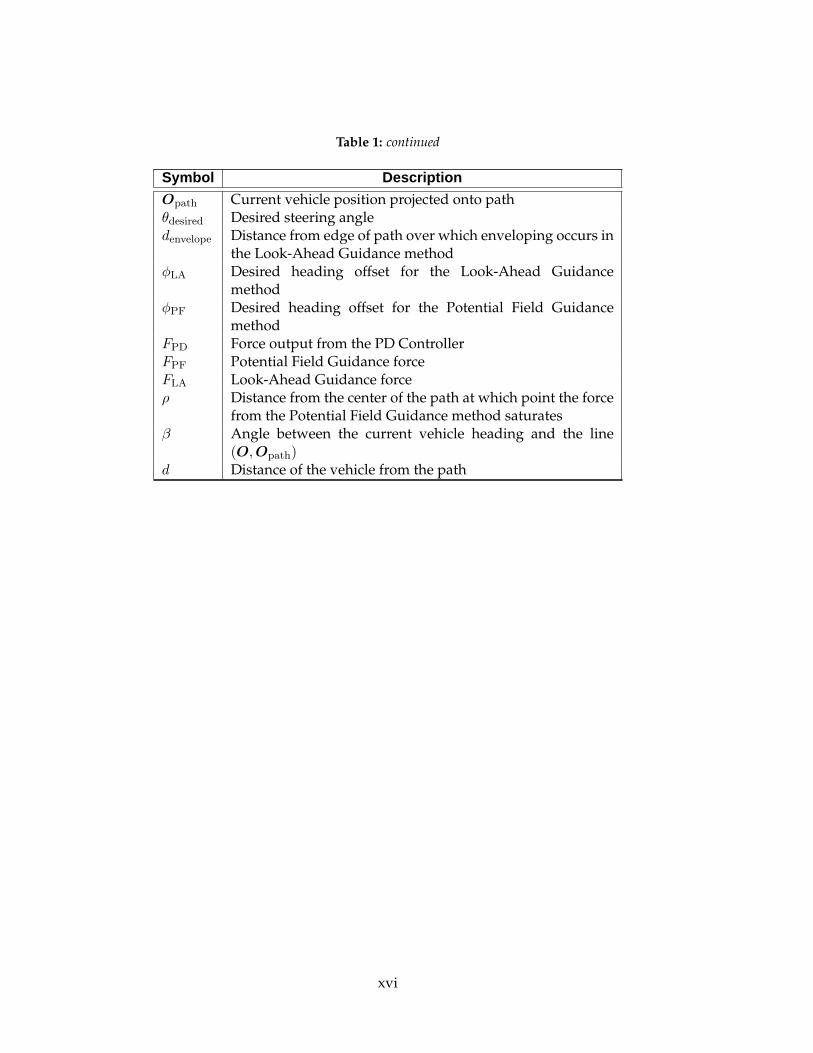
Table 1: continued
Symbol Description
Opath Current vehicle position projected onto pathθdesired Desired steering angledenvelope Distance from edge of path over which enveloping occurs in
the Look-Ahead Guidance methodφLA Desired heading offset for the Look-Ahead Guidance
methodφPF Desired heading offset for the Potential Field Guidance
methodFPD Force output from the PD ControllerFPF Potential Field Guidance forceFLA Look-Ahead Guidance forceρ Distance from the center of the path at which point the force
from the Potential Field Guidance method saturatesβ Angle between the current vehicle heading and the line
(O,Opath)d Distance of the vehicle from the path
xvi
Chapter 1
Introduction
With the spread of intelligent systems in applications as diverse as automobile driving
support, surgical simulation for training, animation design aids and tools for teaching
physical-gestures, haptic force feedback presents an opportunity to enhance highly inter-
active user interfaces. Haptic interfaces can provide intuitive cues derived from an intel-
ligent system’s knowledge of the environment, from a user’s intentions and preferences,
and/or from an assessment of the user’s current capabilities or needs. Many possible ap-
proaches to devising such cues exist, differing in the degree of control retained by the user.
At one extreme, the system can behave autonomously but allow the user limited interven-
tion when desired; at the other, the user is completely responsible for interface control, but
the intelligent system can offer supplementary force suggestions. We have chosen to work
in the space of the latter because we are interested in systems with tightly coupled user
interaction, not semi-autonomous systems.
1.1 Motivation
We were motivated to investigate the problem of effective haptic path guidance while con-
sidering how to use force feedback to assist a user interacting with an intelligent system
that computes constraints on the control space of a dynamic system (such a system is dis-
cussed in Section 2.1). For example, consider a driving simulation as the dynamic system
in question. Then the control space of the system is the acceleration of the vehicle, manip-
1
ulated by the gas and brake pedals, and the steering angle, manipulated by the angular
position of the steering wheel. For simplicity, assign the car a constant velocity and no
acceleration so that the only way to control the system is via the steering wheel. Now
consider an intelligent system that computes the constraints on the steering angle that will
keep the vehicle on the road given the car’s current location, heading and speed. How can
these constraints be conveyed to the driver in an effective and usable way?
We felt that force feedback was an obvious interaction modality to effectively convey
such constraints to the driver. However, our initial attempts to use it did not go well. In
our prototype we used a PHANTOM, a three degree of freedom haptic interface (Massie
and Salisbury, 1994), as the haptic interface to control the steering angle of the simulated
vehicle based on the X-axis position of the end effector, and applied forces to push the end
effector away from constraints. Our difficulty stemmed from the forces being applied too
late and too strongly, thereby abruptly forcing the user away from a constraint and forcing
the interface to the other extreme constraint, resulting in an annoying and ineffective end
effector oscillation. It was easier to control the vehicle with no forces displayed at all than
with our initial attempts at haptically displaying the constraints.
We needed a more subtle approach to make the forces we displayed more useful and
intuitive. We anticipated that by predicting the state of the system and detecting impend-
ing constraint violations (leaving the road) we could apply a force with gently increasing
magnitude to slowly steer the user away from a constraint and thereby avoid the strong,
oscillation-inducing forces we observed in our preliminary work. Ideally, these forces
would be transparent to the user, who would be unaware that forces were being applied
to guide him away from a constraint.
Another possible haptic interaction technique is to display a rigid haptic “wall” to en-
force a constraint rather than to steer the user away from a constraint. A rigidly displayed
constraint would be desirable where it is critical that the user not violate the control con-
straint and where the user is confident that the intelligent system is perfect at calculating
control constraints. If not, the user may become confused and/or annoyed when the sys-
tem computes a non-existent constraint, and/or misses a constraint altogether. We do not
assume that the intelligent system is perfect at computing the control constraints and con-
2
sider problems where the user may want to override the intelligent system’s computed
control constraints. In our approach, the user retains ultimate control, not the intelligent
system.
It is important to note that driving is just one application that could benefit from in-
teraction with control constraints augmented by haptic feedback. Any situation where a
user is navigating a control subspace computed by an intelligent system and can over-
shoot the boundaries of this subspace could benefit from predictive force feedback guid-
ance through the control interface. Such applications include, for example: driving, path
tracing (a common activity for graphic artists), and interactive animation control. For the
sake of simplicity we studied force feedback guidance in a simple driving simulation.
1.2 Objectives and Approach
As touched upon in the previous section, there are many poorly understood human-in-the-
loop considerations for haptic guidance methods. A successful approach will be one that is
intuitive to use, aesthetically acceptable, and does not surprise or annoy the user; it should
make the task at hand easier without being intrusive. The wrong implementation could
result in the user reflexively fighting unexpected forces, relying too heavily on a system
that is not meant to be completely autonomous, or being annoyed rather than aided by the
feedback. Good haptic guidance will not require significant attentional resources from the,
and will have a minimal learning curve, and it will either have a significant quantitative
performance benefit when compared to no haptic feedback, and/or significantly reduce
fatigue and increase user comfort and confidence. We felt that, if properly designed and
implemented, a haptic guidance algorithm based on prediction would address all of these
issues.
We chose to study an application that should yield insights into how haptic guidance
could benefit a larger class of interface problems: a driving simulation where we provide
haptic cues to guide a user along a simulated road. To keep the complexity level reason-
able, the user had control over the vehicle’s steering angle, but not its velocity. This driving
application has a number of useful characteristics:
3
• It is relatively simple; therefore it can be studied in a reasonable amount of time, an
important quality for a Masters thesis project.
• It requires a simple one Degree of Freedom (DoF) haptic interface, a wheel or knob,
which is economical and easy to program compared to higher dimensional haptic
interfaces.
• Steering a car is an under-actuated system, a property shared by some of the other
applications we are interested in such as interactive control of physically based an-
imations. An under-actuated system has more degrees of freedom than there are
degrees of freedom for control. Our driving task is under-actuated because the sys-
tem has three degrees of freedom: position (X and Y values) and orientation (angle
of the vehicle); and one control degree of freedom, the steering wheel angle.
• Most people are familiar with driving; therefore users of our system will require a
minimal amount of time to learn how to use the system. This is important because we
wanted participants in our experiment to spend the majority of their time generating
useful data, not learning how to use the system.
In our experiment, we present to the user a visual representation of a vehicle on a road
by using a modified version of OpenSteer, a vehicle simulation environment developed
by Reynolds (2003) to study intelligent steering behaviours of autonomous vehicles. We
implemented a predictive algorithm, Look-Ahead Guidance, by extending an approach
Reynolds (1999) developed for steering autonomous vehicles along a path. We compare
this to two others, a baseline with No-Guidance force feedback, and a non-predictive, reac-
tive algorithm similar to what we used in our early prototypes mentioned in the previous
section. We refer to the latter as Potential Field Guidance because the forces displayed
are as if the vehicle is in a force field pushing it away from the the edge of the road back
toward the middle of the road. We considered potential field guidance to be the stan-
dard path guidance algorithm when we started this work because many previous haptic
systems used similar methods, as is evident in Chapter 2 on related work.
We describe the design and execution of a formal experiment to quantitatively and
subjectively evaluate the performance of these three haptic guidance methods. We then
4

present our findings with respect to this experiment and discuss how we would proceed
with future work on haptic path guidance.
1.3 Document Map
The remainder of this document puts forward how we addressed the problem of haptic
path guidance and is divided into the following Chapters:
2 - Related Work: This Chapter presents relevant previous work.
3 - Implementation: We present the design and implementation of the haptic path guid-
ance methods that we decided to evaluate, as well as how we modified OpenSteer to
meet the needs of our study.
4 - Evaluation Methods: We present an experimental design to evaluate our guidance meth-
ods in this Chapter.
5 - Experimental Results and Analysis: The process, results and analysis of our experi-
ment are presented in this Chapter.
6 - Discussion: This chapter discusses the work done in the previous three chapters. It
provides details on problems that were encountered, what we could have done bet-
ter, and interesting observations made after the experiment, that were not initially
apparent in the statistical analysis.
7 - Conclusions, Contributions and Future Work: We distill what we learned, present our
contribution to the knowledge in the area of haptic guidance, and what can be done
in the future to learn more about this problem.
5

Chapter 2
Related Work
The use of force feedback to guide users in performing a variety of tasks dates back a
number of years. In one of the earliest examples, Rosenberg (1993) used ‘virtual fixtures’ to
support a teleoperated peg-in-hole task by providing simple guides and constraining entry
to forbidden regions. The haptic guidance work done since can be loosely categorized into
four areas:
• Training
• Non-Training Surgical Applications
• Shared Control of Vehicles
• Path Guidance
2.1 Non-Haptic Control Guidance
Work by Reynolds (1999) on the control of autonomous vehicles provided inspiration for
our Look-Ahead Guidance method. He presents a number of steering behaviors for au-
tonomous vehicles that create realistic, complex behaviors such as flocking, obstacle avoid-
ance and path following. An integral component of his path following algorithm is a pre-
dictor of a vehicle’s position a fixed time interval into the future, which he accomplishes
by using a simple linear algorithm based on the velocity and heading of the vehicle. If the
predicted location of the vehicle is off of the path, then the system commands the vehicle
7
to steer toward the point on the path closest to the predicted location. We call this kind of
predictive path following a look-ahead algorithm.
Reynolds (2003) also developed and made publicly available a software toolkit, Open-
Steer, a test bed for steering behaviors. We used OpenSteer as the basis of our simulation
and rendering engine which saved us the time and effort of developing a similar system
on our own. However, OpenSteer did not satisfy all of our requirements which meant that
we had both to modify parts critical to our study and to accept the drawbacks to some
other, less critical, features such as path representation. In Chapter 3, we discuss in detail
our usage and modifications to OpenSteer.
Look-ahead methods are used by Feng, Tan, Tomizuka, and Zhang (1999) to provide
non-haptic path guidance for driving tasks, especially under low visibility conditions. This
work focuses on the design of a complex vehicle location predictor, and approximations to
this predictor to reduce its computational requirements to the point where the algorithm
can run in real-time. They use a graphical display to present the driver with the predicted
location of the vehicle derived from the approximated location predictor. Feng et al. use a
more complicated vehicle model and predictor than we need. They test their system exper-
imentally, but this is done primarily to verify that their approximated location predictor
algorithm performs well compared to the full algorithm, not to compare the performance
of their system to the performance of driving unaided by their predicted location display.
They also provide some basic experimental results indicating that a larger look-ahead dis-
tance improves path following performance but they do not provide any details on their
experimental procedure and only fleetingly mention the driver’s feelings about using the
system.
Kalisiak and van de Panne (2004) have created an an intelligent system to compute a set
of safe control inputs for a dynamic system which they call viability envelopes. A viability
envelope is the set of control inputs that will keep a dynamic system in a safe state given
the current system state — for instance, the set of steering angles that will keep a driver
in his lane given his current heading and speed. Viability envelopes could also be useful
for helping to control physically-based animations which typically have a small subset
of the entire control space that leads to a ‘good’ animation, such as keeping a character
8
upright while walking. Viability envelopes could be used to make interactive control of
such systems much easier by constraining the control inputs to keep the system in a ‘good’
state. A user of a viability envelope system could potentially realize a large benefit from the
haptic display of the viability envelope since graphical cues may be non-intuitive and/or
distract the user from the task at hand.
2.2 Haptic Training
Haptic feedback has been used to help teach complex motor tasks such as writing Asian
text. The surgical community has several haptic training tools that are primarily used to
simulate the feel of surgery and occasionally to repeat the motions of an expert surgeon.
Teo, Burdet, and Lim (2002) used a 6-DoF haptic device to teach Chinese handwriting.
They model both pen-based writing (2D motions) and calligraphic writing (3D motions).
They employed experts in Chinese writing to record the motions required for a set of char-
acters, which can then be played back to students (spatial and temporal constraint) or
used as a guide (spatial constraint only). Both styles of constraints are implemented with a
slight variation on a simple spring and damper constraint where the haptic interface’s con-
trol point and the closest point on the constraint path to the control point are attached with
a virtual spring and damper. They develop a complicated scoring scheme for a student’s
characters that involves the shape, motion, force and smoothness of their strokes. They do
some basic experiments to measure the quantitative performance of their system via their
score metric and do not formally evaluate the users’ feelings about their interactions with
the system. They report that spatial path constraints without a temporal constraint were
“agreeable to users” and resulted in a performance increase, especially for beginners.
Solis, Avizzano, and Bergamasco (2002) use a custom haptic device to teach the writing
of Japanese characters. The main thrust of their work is in using Hidden Markov Models to
recognize the character that the user is trying to write, and providing haptic path guidance
for that particular character. This contrasts with the work done by Teo et al. which does
no such recognition. The path guidance method employed by Solis et al. is once again a
simple spring and damper method that attempts to keep the control point on the outline
9
of the current character. They evaluate their system by considering the accuracy of their
task recognition algorithm, and they do not look at user interaction issues with the haptic
device or if haptic guidance improves a user’s ability to write Japanese characters. They
evaluate the task recognition of their system on ten different kanji characters, and report
recognition rates varying between 76% and 100%.
Feygin, Keehner, and Tendick (2002) present, and carefully evaluate, a haptic training
method for a perceptual motor skill: tracking the spatial and temporal motion of a point
following a 3D path over time. The trajectory of the point is specified through three 10-
second sinusoidal curves; one for each of the X, Y and Z axes. A PHANTOM is used to
interact with their system. Their experimental task consists of first presenting the trajectory
of the point and then having the user recall the presented trajectory. They have three differ-
ent presentation methods: purely visual (watching the PHANTOM follow the trajectory),
purely haptic (subject cannot see his hand), and simultaneous visual and haptic presenta-
tion; and two recall methods: purely haptic and a combination of haptic and visual. No
active force feedback is presented during recall. The trajectory is presented to the user
by using a simple spring and damper model to guide the user along the trajectory. They
perform a well-designed and detailed experiment with an equally detailed analysis of the
performance of the different presentation and recall methods. They present some interest-
ing metrics for positional, shape and temporal recall accuracy. Our experimental task is
different enough from their task that we cannot use their performance metrics directly, but
we foresee these performance metrics being useful for future haptic path guidance work.
They conclude that “haptic guidance can benefit performance, especially when training
temporal aspects of a task.”
2.3 Haptic Non-Training Surgical Applications
An example of a haptic system used for guiding but not for training a surgical task is
found in the work done by Okamura’s group on virtual fixtures for micro-surgical appli-
cations (Bettini, Lang, Okamura, and Hager, 2001, 2002; Marayong, Bettini, and Okamura,
2002; Marayong, Li, and Allison Okamura, 2003; Marayong and Okamura, 2003). These
10
fixtures provide variable admittance to a user’s input forces which are factored into com-
ponents parallel and perpendicular to a given constraint. The system guides a user along a
constraint by making movement in the direction parallel to the guidance constraint easier
than movement in the perpendicular direction. With this setup, the system can vary the
provided guidance from none to a rigid constraint. Furthermore, the user can be pulled
toward the constraint by making perpendicular motion toward the constraint easier than
away from it. This system is implemented using admittance control, meaning that the
device’s position changes in response to forces exerted on it by a user, as opposed to
impedance control devices, such as ours, which apply forces based on the position of the
device’s end effector.
Okamura’s group has done a number of studies on the performance impact of varying
the amount of guidance provided by the system across a number of different tasks. These
tasks include standard path following, path following while avoiding an obstacle on the
path, and path following with a secondary off-path targeting task. They have also looked
at using machine learning to attempt to identify the different tasks a user is trying to do,
and changing the guidance characteristics appropriately. While we do not look at task
recognition in this thesis, we anticipate that our system would benefit from such function-
ality. As is the case with much of the previous work, this system uses a haptic interface
with at least the same degree of freedom as the system being controlled. Another differ-
ence between this work and ours is that the nature of microsurgical tasks dictates that the
interaction with the haptic device involves very slow motions. This is not a characteristic
of systems where predictive haptic path guidance will be most useful, such as interactive
control of physically-based animation.
2.4 Shared Control of Vehicles
A significant amount of work has been done on active steering in vehicles to help the
driver with tasks such as lane keeping and passing. The majority of the lane keeping work
appears to be motivated by a final goal of autonomous driving, and shared control of the
vehicle is a stepping stone toward that goal.
11
Steele and Gillespie (2001) used haptic guidance in the shared control of a vehicle, and
experimentally examined its effect on visual and cognitive demand. Their path guidance
implementation uses the current lateral displacement of a vehicle from a path to calculate
a desired steering angle “appropriate for good path following”. This is done by applying
a force to the steering wheel proportional to the difference between the desired steering
angle and the current steering angle. This is very similar to our Potential Field Guidance
method described in Section 3.2.4.
They performed two experiments, one designed to test the effect of haptic guidance
on the demand for visual cues, and another to test for the effect of haptic guidance on
a driver’s cognitive processing capacity. In their experiments, a small John Deer tractor
was outfitted with a haptic steering wheel and LCD monitor. Both tasks involved having
a user follow a straight path, with obstacles placed in the middle of the path at various
points along the path length. The participant was given the primary goal of avoiding the
obstacles, and the secondary goal of following the middle of the path as closely as possible.
To measure visual demand in the first task, users saw nothing on the screen until they
pushed a button on the wheel. After pressing this button, they would then, for half a
second, see the simulated environment on the monitor. The number of times the button
was pushed was used to measure the visual demand required to perform the task. This
task was done once with haptic feedback and once without. The authors found that haptic
feedback provided both a significant decrease in visual demand and in lateral deviation
from the path when compared to the no haptic guidance condition.
In the second task, participants were asked to count backwards from 1000 by incre-
ments of 3 while they followed the path and avoided obstacles. They were instructed that
the mental arithmetic was of lower priority than following the path and avoiding obsta-
cles. The authors hypothesized that if haptic guidance affected the cognitive processing
ability of the driver, then there would be a difference in the number of subtractions the
driver could perform with haptic guidance compared to no haptic guidance. They did
not find a significant difference between the number of subtractions performed with or
without haptic guidance.
The components of this study relevant to our work are the use of a similar desired-
12
steering-angle approach to generate control forces, and their finding that haptic guidance
provides a significant reduction in path following error compared to no haptic guidance.
However, they only studied one kind of haptic guidance on a straight path and did not
consider the drivers’ feelings about the haptic guidance compared to no haptic guidance,
something that we believe is necessary for user acceptance of shared control systems.
Rossetter et al. (Rossetter, 2003; Rossetter and Gerdes, 2002a,b; Rossetter, Switkes, and
Gerdes, 2003) employ force feedback potential fields in combination with a look-ahead al-
gorithm to enforce vehicle guidance functions such as lane keeping and general hazard
avoidance. They focus almost completely on safety concerns for implementing lane as-
sistance in a real vehicle. They carefully develop a detailed vehicle model and use this
model to design a mathematically stable lane keeping controller based on a potential field.
To help make their controller stable they needed to add a look-ahead to their potential
field method. This was encouraging information during the development of our system,
because it echoed our experiences with potential field path guidance.
The output of their lane-keeping controller is applied to the steering control of a vehicle
which is shared with the driver via the steering wheel, so that the driver feels the output
of the lane-keeping controller. They made a great effort to ensure that their controller will
keep a car in its lane even in the absence of driver input. This is something that we are
not interested in implementing as we envision a tightly coupled interaction between the
system and the user for our applications, not automation. Only fleetingly in their work
do they discuss the interaction between their system and the driver, mentioning that the
forces feel intuitive without more formally evaluating this observation. In the future work
section of his Ph.D. thesis, Rossetter (2003) acknowledges that user interaction with the
system is an important issue that requires attention in order to create a good path guidance
method. Throughout the design, implementation and evaluation of our system we took
into account the user interaction issues with our system.
13
2.5 Haptic Path Guidance
The majority of existing haptic path guidance work has either been for training or for the
guidance of vehicles. There are some examples of haptic path guidance systems that do
not fall into these categories and we present them in detail here.
Cobots are an example of passive haptic path guidance: the user’s input energy is steered,
dissipated or stored to guide the user along a desired trajectory (Colgate, Wannasuphopra-
sit, and Peshkin, 1996; Swanson and Book, 2003). This is different from every other system
that we have presented so far. Passive haptic guidance is a good candidate when safety is
a primary concern since the haptic interface does not add energy to the system, making it
possible to guarantee stability. This work is not as closely related to our work as some of
the other previous work we have presented but it is an interesting approach to a related
problem.
Another example of a non-vehicle haptic path guidance algorithm is the work done by
Donald and Henle (2000) on the haptic control of animation. Here, high-dimensional mo-
tion capture data is transformed to a three-dimensional trajectory that is interacted with
via a PHANTOM. They present two haptic methods to interact with motion capture data.
In the first method the PHANTOM follows a force ‘river’ around the 3-D trajectory repre-
senting an animation in a high-dimensional configuration space (a 57 degree of freedom
humanoid character). They use a handcrafted transfer function that maps the 3-D config-
uration space to the character’s 57-D configuration space. The user can manipulate the
animation by pushing on the end effector of the PHANTOM, altering its path as it follows
the force river representing the motion capture animation. The PHANTOM is connected
to the animation trajectory via a virtual spring that pulls the end effector toward the trajec-
tory, while another force tries to push the end effector along the trajectory at the pace set
by the motion capture data.
The second interaction method they present is not as direct; the PHANTOM is used
to interact with the force river from the outside instead of by following it. The force river
is rendered as a 3-D tube and can be manipulated with direct haptic feedback from the
PHANTOM. The current temporal position of the animation is indicated by a ball follow-
14

ing the tube. The tubes are designed to feel ‘stretchy’ when manipulated, and the user can
change the shape of the tube by pulling on it with the PHANTOM.
This work presents an interesting way to use a haptic device to interact with higher
dimensional configuration spaces than the interaction device has, and uses paths to ac-
complish this. However, their system is more autonomous than what we would like to
implement and uses a more complicated haptic interface than we would like to use. They
do not perform a user study to analyze the human computer interaction issues with their
system, something that is very important to us and we believe that this requires a simpler
system and task to analyze properly.
15

Chapter 3
Implementation
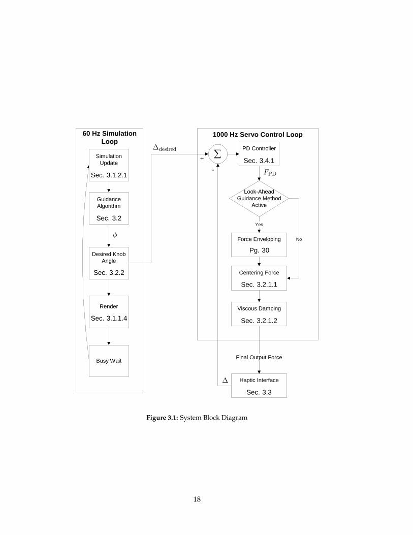
Our system is comprised of several components, depicted in Figure 3.1, which we discuss
in detail throughout this Chapter.
3.1 Simulation and Rendering Engine
In this section we describe how our system simulates and renders a simple virtual envi-
ronment. For the purposes of our experiment, we needed to be able to draw a path and
something resembling a vehicle that a user can control to follow the path on the screen.
The OpenSteer framework by Reynolds (2003) provides a good base set of functionality to-
wards our goals, allowing more time to be spent developing the guidance algorithms and
running experiments than would have been available if we developed everything from
scratch. OpenSteer was designed to help develop intelligent behaviours for autonomous
vehicles, and we extended it to allow for user controlled vehicles with force feedback.
3.1.1 OpenSteer
This section summarizes relevant components of Reynolds’s OpenSteer framework, a basic
simulation and rendering engine. For a complete reference to OpenSteer see its on-line
documentation (Reynolds, 2003). Our changes to OpenSteer are presented in Section 3.1.2.
17
60 Hz SimulationLoop
PD Controller
Look-AheadGuidance Method
Active
Centering Force
Viscous Damping
Haptic Interface
Force Enveloping
Final Output Force
Yes
No
�
-
+
Desired KnobAngle
GuidanceAlgorithm
SimulationUpdate
Render
Busy Wait
1000 Hz Servo Control Loop
Sec. 3.1.2.1
Sec. 3.2
Sec. 3.2.2
Sec. 3.1.1.4
Sec. 3.4.1
Pg. 30
Sec. 3.2.1.1
Sec. 3.2.1.2
Sec. 3.3
∆
∆desired
φ
FPD
Figure 3.1: System Block Diagram
18
3.1.1.1 Path Model
OpenSteer defines an abstract path representation consisting of a radius (1/2 width) and
methods to:
• Get the total length of the path
• Get a point on the path a certain distance from the beginning of the path
• Get the distance along the path of an arbitrary point
• Project a given point onto the path
• Test if a given point is within the radius of the path
Only one concrete implementation of this abstract definition is provided based on a poly-
line, a series of connected line segments.
3.1.1.2 Vehicle Model
OpenSteer’s vehicle model is a very simple one, consisting of a position (which is its center
of mass and rotation), a velocity vector, a radius (size of the vehicle) and mass. The direc-
tion of the velocity vector is always aligned with the heading of the vehicle (i.e. the velocity
vector is always coincident with the center line of the vehicle). The system steers a given
vehicle by applying a 2-D force to the vehicle’s position which in turn affects the vehicle’s
velocity via a physical simulation engine that integrates this force over time. This vehicle
model is inadequate for our needs, and the vehicle model we replace it with is described
in Section 3.1.2.1.
3.1.1.3 Simulation
OpenSteer has three simulation loop steps:
1. Limit simulation update rate (optional).
2. Update the system state.
3. Render.
19

The update rate of the simulation can be limited either by the processor speed or by pur-
posely setting a fixed rate, which is useful for applications such as games that typically
need a fixed update rate. The update rate is limited by doing a busy wait until the next
update time.
The state of the system is updated by iteratively updating the state of each vehicle in
the simulation. A typical vehicle update involves the following steps:
• Calculate a 2-D steering force based on the current state of the vehicle and the rest of
the system.
• Update the vehicle’s velocity by integrating the steering force over the simulation
time-step.
• Use the new vehicle velocity to update the position and orientation of the vehicle.
3.1.1.4 Rendering
After the simulation state has been updated, a visual representation of the new state is
drawn from the point of view of a virtual camera. This camera has a number of possible
behaviors. The default OpenSteer camera behaviours are:
• Static: Render the simulation from a static position and orientation.
• Straight Down: Render the world looking straight down at the selected vehicle from
above. The Y-axis of the view is aligned with the heading of the selected vehicle.
• Fixed Distance Offset: Loosely follow the selected vehicle from a constant distance
and focus on the vehicle.
• Fixed Local Offset: Follow the selected vehicle at a constant position and orientation
offset relative to the vehicle’s coordinate frame.
• Offset Point of View: A view from above and behind the selected vehicle aligned
with the heading of the vehicle and focused on a point a fixed distance ahead of the
vehicle. This is the camera positioning mode that we used for our experiment as it is
similar to the view one would have while driving.
20
Many of the positioning modes depend on a selected vehicle. If the current simulation
contains any vehicles, then there is always exactly one selected vehicle, and if there are
multiple vehicles in the simulation then the user can select a vehicle by clicking on it.
The default visual representation of a vehicle is a solid red triangle inscribed in a white
circle centered at the position of the vehicle. A neighbourhood of the plane around the ve-
hicle is drawn in a checkerboard pattern, which provides visual feedback about the speed
of the vehicle as it moves over the checkerboard. OpenSteer draws paths as a red line, one
pixel in width, and does not draw the full extent of the path.
Overall, OpenSteer is a useful simulation engine for our purposes, but some parts
of OpenSteer needed to be changed to suit our needs. The next section describes these
changes.
3.1.2 OpenSteer Modifications
This section describes the major changes we made to the stock version OpenSteer to sup-
port our work on haptic path guidance. The majority of our changes are to the vehicle
model and the rendering components of OpenSteer. We change the vehicle model and
vehicle simulation algorithm to enable a user to have control of a vehicle’s steering angle.
We change OpenSteer’s rendering of the simulated system to meet the requirements of our
experiment and to reduce the computational resources required for rendering.
3.1.2.1 Vehicle Model and Dynamics
OpenSteer steers a vehicle by applying autonomously computed 2-D force vectors to the
vehicle. We allow users to steer a vehicle in an OpenSteer simulation via a knob. In an
effort to minimize changes to OpenSteer, we attempted to incorporate the user’s input via
the knob with OpenSteer’s existing vehicle steering algorithm. This was accomplished by
applying a force to the vehicle perpendicular to its centerline and with magnitude propor-
tional to the control knob angle. Through some simple tests we found that this method of
enabling user control of a vehicle was not going to work because of problems with how
OpenSteer integrates steering forces over time. Rather than implement a better simula-
tion integration method, we decided to implement a different vehicle model that does not
21
depend on the integration of forces over time.
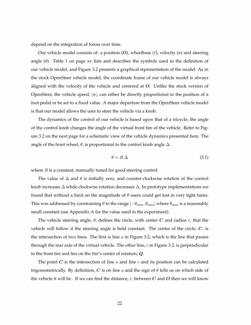
Our vehicle model consists of: a position (O), wheelbase (`), velocity (v) and steering
angle (θ). Table 1 on page xv lists and describes the symbols used in the definition of
our vehicle model, and Figure 3.2 presents a graphical representation of the model. As in
the stock OpenSteer vehicle model, the coordinate frame of our vehicle model is always
aligned with the velocity of the vehicle and centered at O. Unlike the stock version of
OpenSteer, the vehicle speed, |v|, can either be directly proportional to the position of a
foot pedal or be set to a fixed value. A major departure from the OpenSteer vehicle model
is that our model allows the user to steer the vehicle via a knob.
The dynamics of the control of our vehicle is based upon that of a tricycle; the angle
of the control knob changes the angle of the virtual front tire of the vehicle. Refer to Fig-
ure 3.2 on the next page for a schematic view of the vehicle dynamics presented here. The
angle of the front wheel, θ, is proportional to the control knob angle ∆:
θ = R ∆ (3.1)
where R is a constant, manually tuned for good steering control.
The value of ∆ and θ is initially zero, and counter-clockwise rotation of the control
knob increases ∆ while clockwise rotation decreases ∆. In prototype implementations we
found that without a limit on the magnitude of θ users could get lost in very tight turns.
This was addressed by constraining θ to the range [−θmax, θmax] where θmax is a reasonably
small constant (see Appendix A for the value used in the experiment).
The vehicle steering angle, θ, defines the circle, with center C and radius r, that the
vehicle will follow if the steering angle is held constant. The center of the circle, C, is
the intersection of two lines. The first is line a in Figure 3.2, which is the line that passes
through the rear axle of the virtual vehicle. The other line, c in Figure 3.2, is perpendicular
to the front tire and lies on the tire’s center of rotation, Q.
The point C is the intersection of line a and line c and its position can be calculated
trigonometrically. By definition, C is on line a and the sign of θ tells us on which side of
the vehicle it will be . If we can find the distance, r, between C and O then we will know
22
`
r
a
b
c
θ
θ
O
v
C
Q
Figure 3.2: Schematic of Vehicle Dynamics: shaded area represents the vehicle itself.
the position of C exactly. By trigonometry 6 OCQ = θ and then,
r =
`
tan θ : θ 6= 0
∞ : θ = 0.
(3.2)
The dynamics of our vehicle model is different from OpenSteer’s. We do not integrate
a steering force every simulation step, but instead move our vehicle along the circle (C, r)
according to its speed. The parameters of the circle are computed at the beginning of each
step using Equation 3.2. The simulation update rate is 60 Hz; therefore the distance that the
vehicle moves each simulation step is |v| 160 . If 0 ≤ |θ| ≤ 0.05◦ then the vehicle moves this
distance in a straight line, otherwise the vehicle moves this distance along the circle (C, r)
from the position of point O at the beginning of the simulation step. To finish the vehicle
update, the direction of the vehicle’s velocity is modified to be in the same direction as the
tangent to the circle at the vehicle’s new position.
This vehicle model and dynamics are sufficient for the requirements of our work: a
simple vehicle simulation that can be intuitively controlled via a knob. The model is not
physically accurate because apart from the development time, exact physical accuracy is
not critical to understanding the general performance and utility of haptic guidance meth-
ods.
23
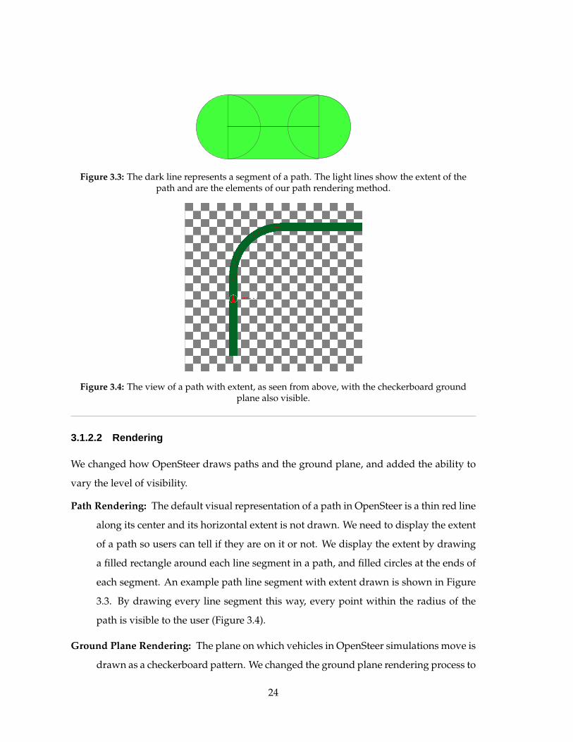
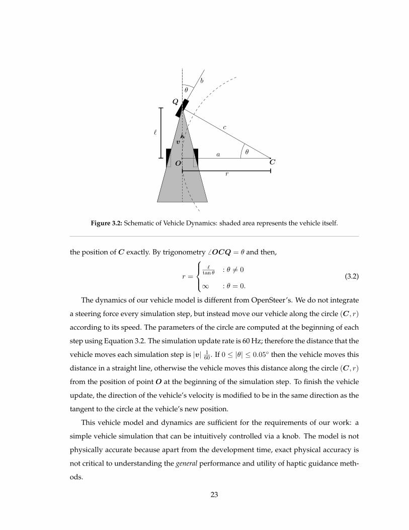
Figure 3.3: The dark line represents a segment of a path. The light lines show the extent of thepath and are the elements of our path rendering method.
Figure 3.4: The view of a path with extent, as seen from above, with the checkerboard groundplane also visible.
3.1.2.2 Rendering
We changed how OpenSteer draws paths and the ground plane, and added the ability to
vary the level of visibility.
Path Rendering: The default visual representation of a path in OpenSteer is a thin red line
along its center and its horizontal extent is not drawn. We need to display the extent
of a path so users can tell if they are on it or not. We display the extent by drawing
a filled rectangle around each line segment in a path, and filled circles at the ends of
each segment. An example path line segment with extent drawn is shown in Figure
3.3. By drawing every line segment this way, every point within the radius of the
path is visible to the user (Figure 3.4).
Ground Plane Rendering: The plane on which vehicles in OpenSteer simulations move is
drawn as a checkerboard pattern. We changed the ground plane rendering process to
24
use textures instead of OpenGL geometry because modern graphics accelerator cards
can draw textures very quickly and the texture can repeat to infinity. The ground
plane in the stock version of OpenSteer was only drawn in a small neighbourhood
around the vehicle because of the large computational demands required to draw a
larger ground plane with OpenGL geometry. To ensure the best visual quality of the
ground plane rendering we employ anisotropic filtering (Everitt, 2000).
Fog: One of the independent variables in our experiment (described in Chapter 4) is the
level of visibility. We change the level of visibility in OpenSteer simulations by using
OpenGL fog, specifically the GL EXP2 exponential fog method (Woo and Shreiner,
2003) where the density of the fog increases exponentially with distance from the
viewpoint. The color of the fog can be set to any 24 bit RGB value, and we use a dark
grey with RGB values (0.3, 0.3, 0.3).
These are the major changes that we made to OpenSteer which we then used to develop
our path guidance methods and perform our experiment.
3.2 Guidance Algorithms
This section presents how we compute forces for our haptic guidance methods and which
forces are present in the baseline “No-Guidance” method. The two active haptic path
guidance methods we implement are Potential Field Guidance and Look-Ahead Guidance.
A pure potential field haptic path guidance method calculates guidance forces based solely
upon the distance between the vehicle and the path. A look-ahead method, on the other
hand, computes guidance forces based upon a predicted future position of the vehicle.
3.2.1 Forces Common to All Guidance Methods
During the iterative development of the guidance methods described in Sections 3.2.3 and
3.2.4, we introduced a centering force and a viscous damping force for the sake of usability.
These forces are present in each method, and they increase the usability of our system both
through positive transfer, they make the interaction with the control knob more like the
interaction with a real steering wheel, and by increasing the stability of the interaction.
25
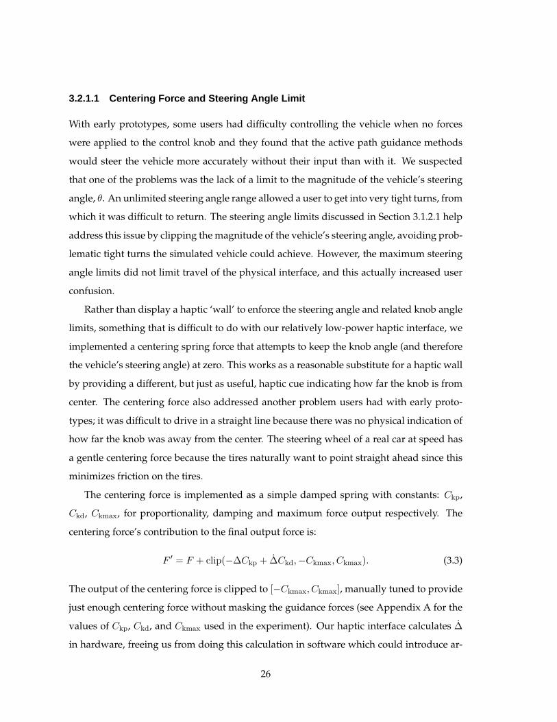
3.2.1.1 Centering Force and Steering Angle Limit
With early prototypes, some users had difficulty controlling the vehicle when no forces
were applied to the control knob and they found that the active path guidance methods
would steer the vehicle more accurately without their input than with it. We suspected
that one of the problems was the lack of a limit to the magnitude of the vehicle’s steering
angle, θ. An unlimited steering angle range allowed a user to get into very tight turns, from
which it was difficult to return. The steering angle limits discussed in Section 3.1.2.1 help
address this issue by clipping the magnitude of the vehicle’s steering angle, avoiding prob-
lematic tight turns the simulated vehicle could achieve. However, the maximum steering
angle limits did not limit travel of the physical interface, and this actually increased user
confusion.
Rather than display a haptic ‘wall’ to enforce the steering angle and related knob angle
limits, something that is difficult to do with our relatively low-power haptic interface, we
implemented a centering spring force that attempts to keep the knob angle (and therefore
the vehicle’s steering angle) at zero. This works as a reasonable substitute for a haptic wall
by providing a different, but just as useful, haptic cue indicating how far the knob is from
center. The centering force also addressed another problem users had with early proto-
types; it was difficult to drive in a straight line because there was no physical indication of
how far the knob was away from the center. The steering wheel of a real car at speed has
a gentle centering force because the tires naturally want to point straight ahead since this
minimizes friction on the tires.
The centering force is implemented as a simple damped spring with constants: Ckp,
Ckd, Ckmax, for proportionality, damping and maximum force output respectively. The
centering force’s contribution to the final output force is:
F ′ = F + clip(−∆Ckp + ∆Ckd,−Ckmax, Ckmax). (3.3)
The output of the centering force is clipped to [−Ckmax, Ckmax], manually tuned to provide
just enough centering force without masking the guidance forces (see Appendix A for the
values of Ckp, Ckd, and Ckmax used in the experiment). Our haptic interface calculates ∆
in hardware, freeing us from doing this calculation in software which could introduce ar-
26
tifacts into the force output (similar differentiation artifacts are discussed in Section 3.4.1).
3.2.1.2 Viscous Damping
To improve the ‘feel’ of the force feedback, and to help smooth the output signal of the PD
controller described in section 3.4.1, we added a viscous damping component to the force
output. This viscous damping is proportional to the angular velocity of the control knob
and its contribution to the overall output force is defined as follows:
F ′ = F − kv ∆. (3.4)
Informal experimentation indicated that these two force components improved the us-
ability and feel of our interface considerably. They provide a good base feeling for the
haptic interface on which to layer the path guidance forces.
3.2.2 Desired Steering Angle Algorithm and Force Output
Before it is possible to describe the haptic path guidance methods in detail, it is useful to
understand a little bit about the process these algorithms use to have a force displayed to
the control knob. The low-level force control for the haptic interface is a PD controller on
the angular position of the control knob (described in Section 3.4). The Look-Ahead Guid-
ance and Potential Field Guidance methods compute a desired vehicle direction, which is
first transformed into a desired steering angle; and then to the desired angular position of
the knob, which is given to the PD controller. The ultimate goal is to reduce the difference
between the current and the desired vehicle heading by steering the vehicle towards the
desired heading.
The guidance algorithms described in the following two sections express the desired
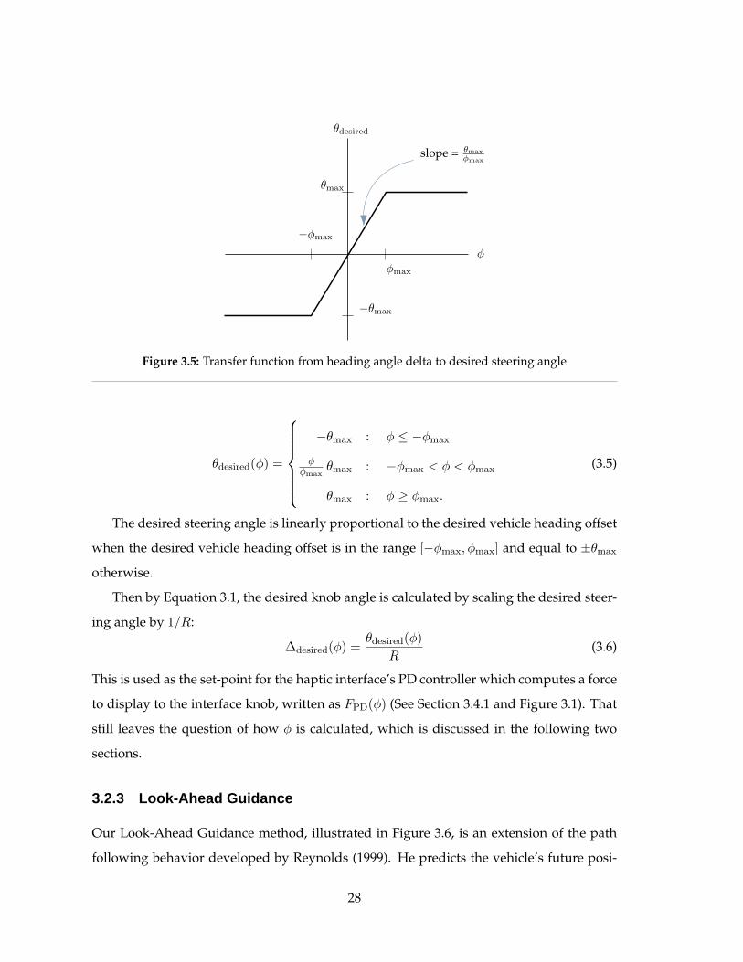
vehicle heading as an offset from the current vehicle heading, φ. Equation 3.5 shows how
the desired steering angle, θdesired, is a function of the desired heading offset, φ, and Fig-
ure 3.5 illustrates this function. The reader may wish to refer to Table 1 on page xv, the
reference to symbol definitions.
27
θdesired
φ
θmax
−θmax
φmax
−φmax
slope = θmax
φmax
Figure 3.5: Transfer function from heading angle delta to desired steering angle
θdesired(φ) =
−θmax : φ ≤ −φmax
φφmax
θmax : −φmax < φ < φmax
θmax : φ ≥ φmax.
(3.5)
The desired steering angle is linearly proportional to the desired vehicle heading offset
when the desired vehicle heading offset is in the range [−φmax, φmax] and equal to ±θmax
otherwise.
Then by Equation 3.1, the desired knob angle is calculated by scaling the desired steer-
ing angle by 1/R:
∆desired(φ) =θdesired(φ)
R(3.6)
This is used as the set-point for the haptic interface’s PD controller which computes a force
to display to the interface knob, written as FPD(φ) (See Section 3.4.1 and Figure 3.1). That
still leaves the question of how φ is calculated, which is discussed in the following two
sections.
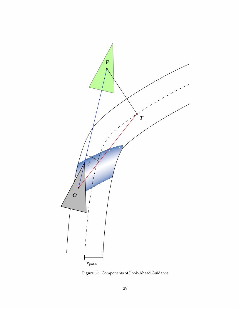
3.2.3 Look-Ahead Guidance
Our Look-Ahead Guidance method, illustrated in Figure 3.6, is an extension of the path
following behavior developed by Reynolds (1999). He predicts the vehicle’s future posi-
28
O
φ
P
T
rpath
Figure 3.6: Components of Look-Ahead Guidance
29
denveloperpath
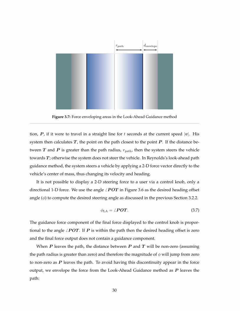
Figure 3.7: Force enveloping areas in the Look-Ahead Guidance method
tion, P , if it were to travel in a straight line for t seconds at the current speed |v|. His
system then calculates T , the point on the path closest to the point P . If the distance be-
tween T and P is greater than the path radius, rpath, then the system steers the vehicle
towards T ; otherwise the system does not steer the vehicle. In Reynolds’s look-ahead path
guidance method, the system steers a vehicle by applying a 2-D force vector directly to the
vehicle’s center of mass, thus changing its velocity and heading.
It is not possible to display a 2-D steering force to a user via a control knob, only a
directional 1-D force. We use the angle 6 POT in Figure 3.6 as the desired heading offset
angle (φ) to compute the desired steering angle as discussed in the previous Section 3.2.2.
φLA = 6 POT . (3.7)
The guidance force component of the final force displayed to the control knob is propor-
tional to the angle 6 POT . If P is within the path then the desired heading offset is zero
and the final force output does not contain a guidance component.
When P leaves the path, the distance between P and T will be non-zero (assuming
the path radius is greater than zero) and therefore the magnitude of φ will jump from zero
to non-zero as P leaves the path. To avoid having this discontinuity appear in the force
output, we envelope the force from the Look-Ahead Guidance method as P leaves the
path:
30
FLA(φLA) = FPD(φLA) ·
0 : |P − T | < rpath
( |P−T |−rpath
denvelope)2 : Otherwise
1 : |P − T | > rpath + denvelope
(3.8)
where denvelope is the distance past the edge over which force enveloping occurs. A graphi-
cal depiction of the force enveloping components can be seen in Figure 3.7 on the preceding
page.
3.2.3.1 Look-Ahead Position Predictor Improvements
Our current Look-Ahead Guidance method uses a simple linear method to predict the
location of the vehicle t seconds into the future, multiplying the current vehicle velocity
by t and adding this to the vehicle position. This predictor is accurate when the vehicle is
moving in a straight line, but incorrect if the vehicle is in a turn.
A more intelligent predictor has the potential to be more accurate across a wider range
of vehicle behaviors than for one merely traveling in a straight line. For example, the
position predictor could consider the movement of the vehicle in the recent past, or the
predictor could look at the current turning radius of the vehicle to more accurately predict
the future position of a vehicle while in a turn.
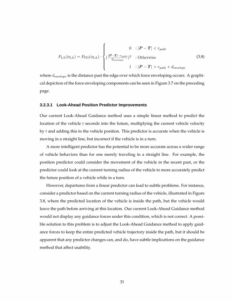
However, departures from a linear predictor can lead to subtle problems. For instance,
consider a predictor based on the current turning radius of the vehicle, illustrated in Figure
3.8, where the predicted location of the vehicle is inside the path, but the vehicle would
leave the path before arriving at this location. Our current Look-Ahead Guidance method
would not display any guidance forces under this condition, which is not correct. A possi-
ble solution to this problem is to adjust the Look-Ahead Guidance method to apply guid-
ance forces to keep the entire predicted vehicle trajectory inside the path, but it should be
apparent that any predictor changes can, and do, have subtle implications on the guidance
method that affect usability.
31
Linear
Predictor
Non-Linear
Predictor
Figure 3.8: An example of the subtleties involved with advanced location predictors
3.2.4 Potential Field Guidance
It is difficult to implement a haptic potential field guidance method with a one degree of
freedom (DoF) haptic interface. We define potential field guidance as a force dependent
only upon the distance of the vehicle from the path. With a two DoF haptic interface, one
can apply a 2-D force pushing the end-effector of the haptic interface towards the center
of the path. With a one DoF haptic interface such as ours, one can only apply a force to
change the steering angle of the vehicle, and we found that the simple algorithm of apply-
ing a raw force proportional to the distance from the path was unstable and hard to use.
We create a more usable, one DoF potential field guidance force that is proportional to the
distance between the vehicle and the path, up to a maximum force at a distance ρ from
the path. We create this force by computing an artificial desired heading offset, φpf , that is
proportional to the distance of the vehicle from the path. By taking advantage of the rela-
tionship between φpf and the magnitude of the PD controller output force, FPD(φpf) (see
Equations 3.5, 3.6, and 3.13), we are able to produce a stable guidance force proportional
to the distance from the path.
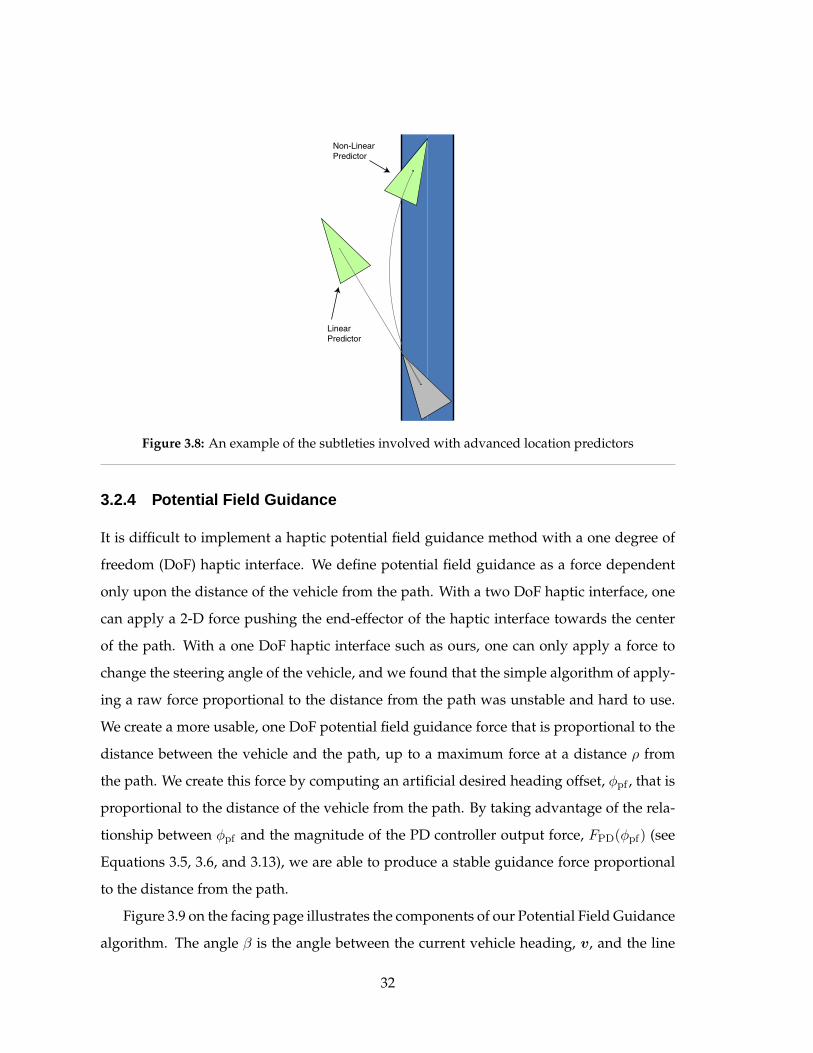
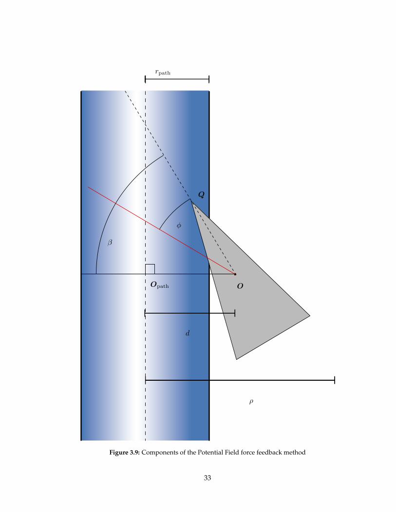
Figure 3.9 on the facing page illustrates the components of our Potential Field Guidance
algorithm. The angle β is the angle between the current vehicle heading, v, and the line
32
O
φ
β
d
Q
Opath
rpath
ρ
Figure 3.9: Components of the Potential Field force feedback method
33
between the location of the vehicle, O, to the point on the path closest to the vehicle, Opath.
This angle is negative if Q is to the left of the line (O,Opath) and positive if Q is to the
right of this line. The angle β is important because it represents the vehicle heading offset
required to head straight back to the path. We do not want the desired heading offset,
φpf , to be greater than β because this will result in non-intuitive guidance forces; the PD
controller will apply guidance forces to achieve a vehicle heading that is beyond the line
straight back to the path. Now we can describe the mathematical derivation of the artificial
desired heading offset, φpf , for the Potential Field Guidance method as a function of the
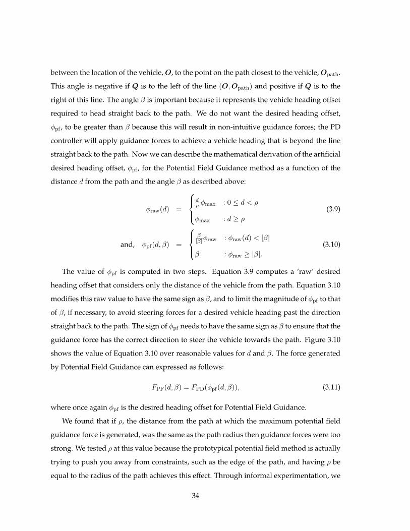
distance d from the path and the angle β as described above:
φraw(d) =
dρ φmax : 0 ≤ d < ρ
φmax : d ≥ ρ
(3.9)
and, φpf(d, β) =
β|β|φraw : φraw(d) < |β|
β : φraw ≥ |β|.(3.10)
The value of φpf is computed in two steps. Equation 3.9 computes a ‘raw’ desired
heading offset that considers only the distance of the vehicle from the path. Equation 3.10
modifies this raw value to have the same sign as β, and to limit the magnitude of φpf to that
of β, if necessary, to avoid steering forces for a desired vehicle heading past the direction
straight back to the path. The sign of φpf needs to have the same sign as β to ensure that the
guidance force has the correct direction to steer the vehicle towards the path. Figure 3.10
shows the value of Equation 3.10 over reasonable values for d and β. The force generated
by Potential Field Guidance can expressed as follows:
FPF(d, β) = FPD(φpf(d, β)), (3.11)
where once again φpf is the desired heading offset for Potential Field Guidance.
We found that if ρ, the distance from the path at which the maximum potential field
guidance force is generated, was the same as the path radius then guidance forces were too
strong. We tested ρ at this value because the prototypical potential field method is actually
trying to push you away from constraints, such as the edge of the path, and having ρ be
equal to the radius of the path achieves this effect. Through informal experimentation, we
34
-200
-100
0
100
200
-2
-1
0
1
2
-100
-50
0
50
100
φ
d
β
Figure 3.10: Values of φ for a given d and β.
found that when ρ was twice as large as the path radius the potential field guidance forces
felt ‘good’.
3.3 Haptic Interface Device
We used a number of different haptic interfaces during the development of our haptic path
guidance system. Initial prototyping was done using a “Twiddler” (Shaver and MacLean,
2003), an inexpensive one DoF haptic interface developed in our lab. We evaluated a com-
mercial haptic gaming steering wheel to use as our haptic interface but found it was not
controllable enough for our needs. We did not have the time or resources to build an
ideal custom solution so we conducted the experiment using the highest quality one DoF
interface available in our lab.
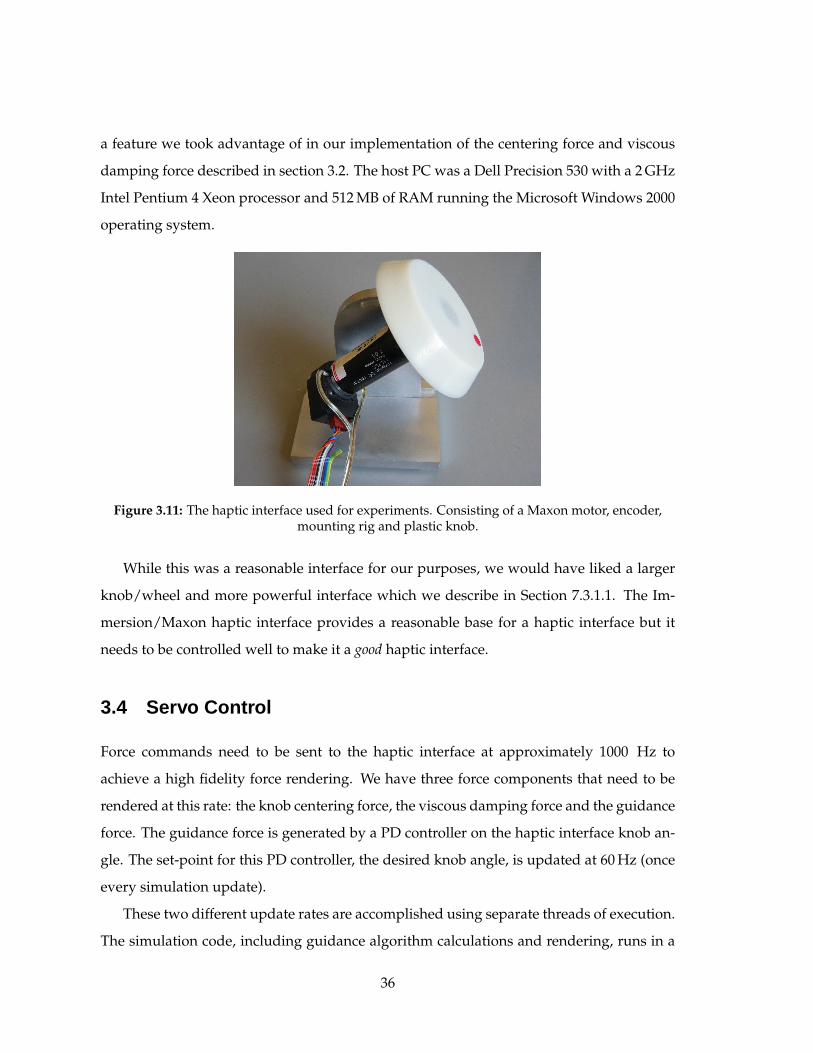
The haptic interface that we used for the final development phase and the experiments
consisted of a 20 W Maxon motor with a 4000 counts per revolution encoder mounted on
a custom aluminum rig. The shaft of the motor is directly attached to a plastic, beveled-
edge knob, 9 cm in diameter. Figure 3.11 shows the motor, knob, and mounting rig as
they were configured for development and experiments. The knob interfaces with the
computer via an Immersion data acquisition PCI board and associated amplifier board,
the Impulse Drive Board 1.0. This board calculates the velocity of the knob in hardware,
35
a feature we took advantage of in our implementation of the centering force and viscous
damping force described in section 3.2. The host PC was a Dell Precision 530 with a 2 GHz
Intel Pentium 4 Xeon processor and 512 MB of RAM running the Microsoft Windows 2000
operating system.
Figure 3.11: The haptic interface used for experiments. Consisting of a Maxon motor, encoder,mounting rig and plastic knob.
While this was a reasonable interface for our purposes, we would have liked a larger
knob/wheel and more powerful interface which we describe in Section 7.3.1.1. The Im-
mersion/Maxon haptic interface provides a reasonable base for a haptic interface but it
needs to be controlled well to make it a good haptic interface.
3.4 Servo Control
Force commands need to be sent to the haptic interface at approximately 1000 Hz to
achieve a high fidelity force rendering. We have three force components that need to be
rendered at this rate: the knob centering force, the viscous damping force and the guidance
force. The guidance force is generated by a PD controller on the haptic interface knob an-
gle. The set-point for this PD controller, the desired knob angle, is updated at 60 Hz (once
every simulation update).
These two different update rates are accomplished using separate threads of execution.
The simulation code, including guidance algorithm calculations and rendering, runs in a
36
normal priority thread at 60 Hz which is maintained by using a busy wait if necessary. The
force rendering code runs at 1000 Hz in a separate thread created with the highest prior-
ity for user threads in Windows 2000. Due to the priority difference between these two
threads, the force rendering thread will pre-empt the simulation thread if necessary, which
is why a busy wait can be used to limit the update rate of the simulation thread. How-
ever, this means that if the execution of the force rendering code takes too long, not only
could the force rendering loop not run at 1000 Hz and cause haptic artifacts, but it could
also starve the simulation thread, resulting in choppy simulation rendering and choppy
desired knob angle calculations. Care must then be taken to ensure that the force render-
ing code is efficient, and that each update takes less than one millisecond to maintain a
1000 Hz update rate.
Figure 3.1 on page 18 is a block diagram of the entire system and is useful to help
understand how the different components of the system fit together. The PD controller is
an important component of our system as the source of the actual guidance forces, and
deserves a detailed discussion.
3.4.1 PD Controller
A PD controller attempts to minimize the difference between a set-point and a process
variable; our process variable is the current knob angle, ∆, and our set-point is the desired
knob angle, ∆desired. It attempts to reduce the difference ∆desired − ∆ by applying a force
to the control knob that is proportional to both the difference and the rate of change of the
difference. The equation for our PD controller is as follows:
ε(φ) = ∆desired(φ)−∆ (3.12)
FPD(φ) = kp ε(φ)− kd ε(φ) (3.13)
where kp is the constant of proportionality and kd is the differential constant. The value of
these constants during the experiments can be found in Appendix A.
Calculating ε smoothly is difficult because ε comes from an encoder reading, ∆. It is
known that it is difficult to differentiate encoder values using finite difference methods
37
(Belanger, 1992), as we found out when attempted to estimate ε using a finite difference
method over several time steps as follows:
ε(φn) =ε(φn)− ε(φn−r)
tn − tn−r(3.14)
We tested this method with values of r in the range [1, 5] and found that this method
produces unacceptable vibrations in our PD controller output, especially when ε is small.
A simple low pass filter to smooth out the ε signal before differentiation did little to help
reduce vibrations. We could have used the angular velocity of the knob angle, ∆, from
the Immersion Impulse Board (see Section 3.3) in our calculation of ε, but we had finished
implementing our PD controller before we started using the Impulse Board and did not
have time to go back and update the implementation to take advantage of this.
We used a variable windowing algorithm developed by Janabi-Sharifi, Hayward, and
Chen (2000) to differentiate ε. This method was developed to calculate the velocity of a
position encoder which we applied to our problem of computing the rate of change of ε.
Their algorithm uses a finite difference method with an adaptive time window to differen-
tiate position encoder readings over a wide range of velocities. They present a number of
additions to their basic method to improve its performance, but we found that the most
basic method which they call end-fit first-order adaptive windowing (end-fit-FOAW) was suf-
ficient for our needs. We followed their suggestion to use a median filter on the output
signal (ε) to eliminate fine irregularities and outliers in the signal while preserving input
signal discontinuities. This method of calculating ε significantly reduced the vibration in
our system from the PD controller.
3.5 Summary
This chapter presented our implementation of two different haptic path guidance algo-
rithms using a simple one DoF haptic interface. We first developed a simulation environ-
ment to present to the user a path to follow, which was done with the help of the OpenSteer
library developed by Reynolds. Users interact with this environment via a one DoF inter-
face that controls a simulated vehicle. We evaluated three different haptic interfaces and
settled with one that was not exactly what we wanted, but was adequate for our needs.
38

No existing commercially available haptic interfaces met our criteria for form factor, power
and controllability. We implemented two haptic path guidance algorithms: Potential Field
Guidance and Look-Ahead Guidance, to display path guidance forces to a user via our
haptic interface. We will now describe how we designed and executed an experiment to
evaluate the performance of these guidance algorithms.
39

Chapter 4
Evaluation Methods
In this Chapter we present our hypotheses about haptic path guidance and an experimen-
tal design to test these hypotheses.
4.1 Hypotheses
We hypothesized the following about the performance of our haptic path guidance meth-
ods:
• Look-Ahead Guidance will have measurable performance benefits over our
No-Guidance baseline.
• Look-Ahead Guidance will have measurable performance benefits over Potential
Field Guidance.
• Look-Ahead Guidance will perform well across a range of path complexities.
• Look-Ahead Guidance will perform well over a range of visibility conditions.
• Users will subjectively prefer the Look-Ahead Guidance to Potential Field Guidance
and the baseline of No-Guidance.
We designed an experiment to test our hypotheses and performed two small pilot stud-
ies before a full scale experiment. The pilot studies were useful in helping us refine our
experimental design and procedure for the full experiment.
41
4.2 Design
This section presents the procedural and statistical design of the experiment we used to test
the hypotheses presented above. We considered many different independent variables to
explicitly control, and chose three to study in our final experiment. We ran two pilot stud-
ies to refine our experimental design before running a formal experiment. The experiment
was designed with the target completion time of approximately one hour. Within this
hour we wanted each participant to see each of the unique combinations of the levels of
the independent variables at least three times, to achieve an improved estimate of actual
performance than that provided by a single repetition. The final design of our experiment
was a 3× 3× 2 within-subject design, with five repetitions of each of the eighteen unique
combinations of the levels of the independent variables.
4.2.1 Choice of Independent Variables
We considered over twelve different independent variables which might affect path fol-
lowing performance. We narrowed these twelve down to those we considered the most
interesting: guidance method, path complexity and visibility. Table 4.1 on page 44 summa-
rizes the levels of the factors we chose to study and we will now describe these in detail.
Guidance Method: It was necessary to study guidance method, because it is our primary
focus, but choosing the number and identity of the comparison cases was difficult.
We decided to compare Look-Ahead Guidance to No-Guidance as a baseline, and
Potential Field Guidance which we considered to be an instance of the standard path
guidance method based on the previous work we presented in Chapter 2. The No-
Guidance method does present some force feedback to the user for the sake of us-
ability as discussed in Section 3.2.1 but does not present any guidance forces. We
considered comparing the Look-Ahead Guidance method to the potential field guid-
ance method by Rossetter et al.(Rossetter, 2003; Rossetter and Gerdes, 2002a,b; Ros-
setter et al., 2003), but time did not permit such a comparison, because it would have
taken a significant amount of time to implement their vehicle model and simulation
dynamics.
42
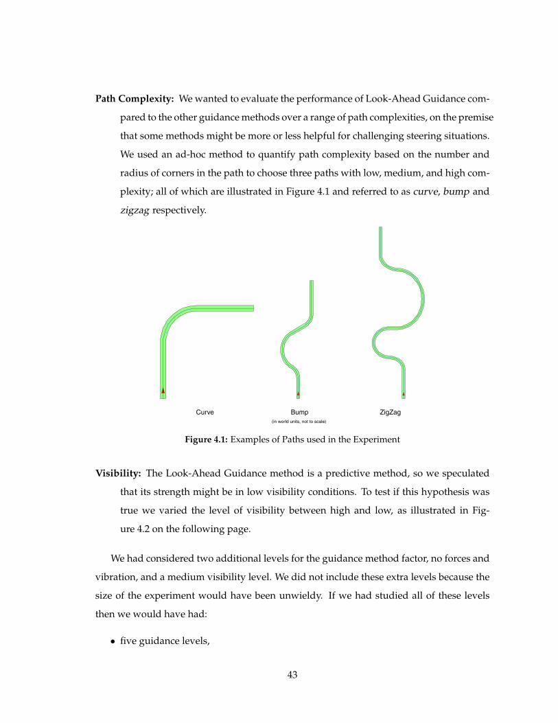
Path Complexity: We wanted to evaluate the performance of Look-Ahead Guidance com-
pared to the other guidance methods over a range of path complexities, on the premise
that some methods might be more or less helpful for challenging steering situations.
We used an ad-hoc method to quantify path complexity based on the number and
radius of corners in the path to choose three paths with low, medium, and high com-
plexity; all of which are illustrated in Figure 4.1 and referred to as curve, bump and
zigzag respectively.
BumpCurve ZigZag
(in world units, not to scale)
Figure 4.1: Examples of Paths used in the Experiment
Visibility: The Look-Ahead Guidance method is a predictive method, so we speculated
that its strength might be in low visibility conditions. To test if this hypothesis was
true we varied the level of visibility between high and low, as illustrated in Fig-
ure 4.2 on the following page.
We had considered two additional levels for the guidance method factor, no forces and
vibration, and a medium visibility level. We did not include these extra levels because the
size of the experiment would have been unwieldy. If we had studied all of these levels
then we would have had:
• five guidance levels,
43
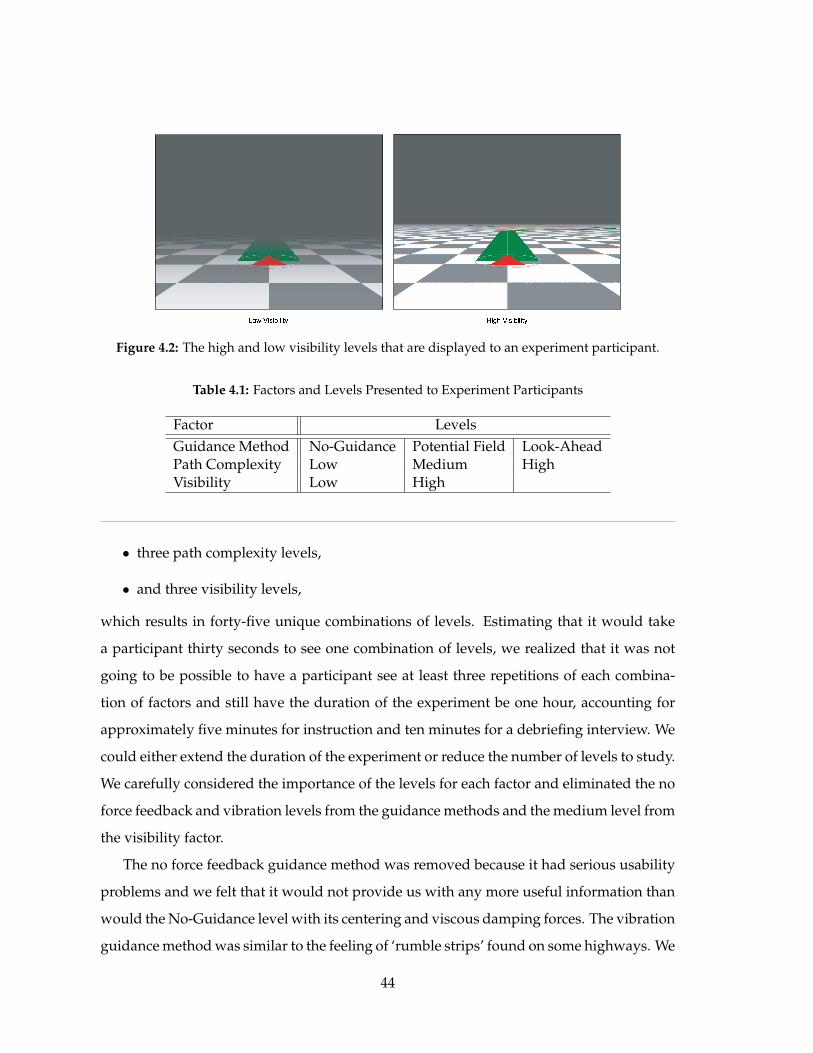
������������ ������������
Figure 4.2: The high and low visibility levels that are displayed to an experiment participant.
Table 4.1: Factors and Levels Presented to Experiment Participants
Factor LevelsGuidance Method No-Guidance Potential Field Look-AheadPath Complexity Low Medium HighVisibility Low High
• three path complexity levels,
• and three visibility levels,
which results in forty-five unique combinations of levels. Estimating that it would take
a participant thirty seconds to see one combination of levels, we realized that it was not
going to be possible to have a participant see at least three repetitions of each combina-
tion of factors and still have the duration of the experiment be one hour, accounting for
approximately five minutes for instruction and ten minutes for a debriefing interview. We
could either extend the duration of the experiment or reduce the number of levels to study.
We carefully considered the importance of the levels for each factor and eliminated the no
force feedback and vibration levels from the guidance methods and the medium level from
the visibility factor.
The no force feedback guidance method was removed because it had serious usability
problems and we felt that it would not provide us with any more useful information than
would the No-Guidance level with its centering and viscous damping forces. The vibration
guidance method was similar to the feeling of ‘rumble strips’ found on some highways. We
44
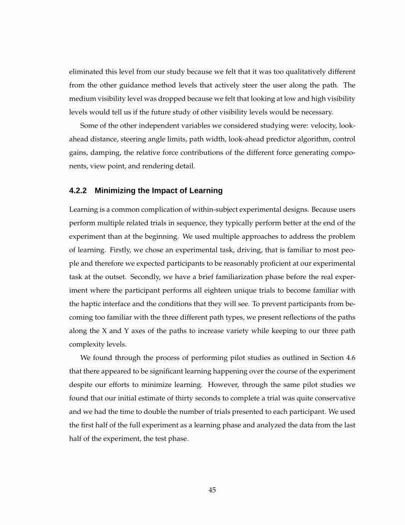
eliminated this level from our study because we felt that it was too qualitatively different
from the other guidance method levels that actively steer the user along the path. The
medium visibility level was dropped because we felt that looking at low and high visibility
levels would tell us if the future study of other visibility levels would be necessary.
Some of the other independent variables we considered studying were: velocity, look-
ahead distance, steering angle limits, path width, look-ahead predictor algorithm, control
gains, damping, the relative force contributions of the different force generating compo-
nents, view point, and rendering detail.
4.2.2 Minimizing the Impact of Learning
Learning is a common complication of within-subject experimental designs. Because users
perform multiple related trials in sequence, they typically perform better at the end of the
experiment than at the beginning. We used multiple approaches to address the problem
of learning. Firstly, we chose an experimental task, driving, that is familiar to most peo-
ple and therefore we expected participants to be reasonably proficient at our experimental
task at the outset. Secondly, we have a brief familiarization phase before the real exper-
iment where the participant performs all eighteen unique trials to become familiar with
the haptic interface and the conditions that they will see. To prevent participants from be-
coming too familiar with the three different path types, we present reflections of the paths
along the X and Y axes of the paths to increase variety while keeping to our three path
complexity levels.
We found through the process of performing pilot studies as outlined in Section 4.6
that there appeared to be significant learning happening over the course of the experiment
despite our efforts to minimize learning. However, through the same pilot studies we
found that our initial estimate of thirty seconds to complete a trial was quite conservative
and we had the time to double the number of trials presented to each participant. We used
the first half of the full experiment as a learning phase and analyzed the data from the last
half of the experiment, the test phase.
45
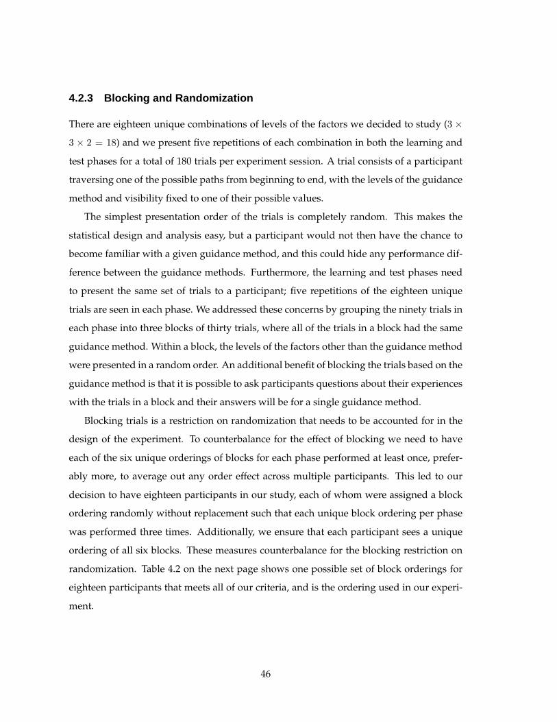
4.2.3 Blocking and Randomization
There are eighteen unique combinations of levels of the factors we decided to study (3 ×
3 × 2 = 18) and we present five repetitions of each combination in both the learning and
test phases for a total of 180 trials per experiment session. A trial consists of a participant
traversing one of the possible paths from beginning to end, with the levels of the guidance
method and visibility fixed to one of their possible values.
The simplest presentation order of the trials is completely random. This makes the
statistical design and analysis easy, but a participant would not then have the chance to
become familiar with a given guidance method, and this could hide any performance dif-
ference between the guidance methods. Furthermore, the learning and test phases need
to present the same set of trials to a participant; five repetitions of the eighteen unique
trials are seen in each phase. We addressed these concerns by grouping the ninety trials in
each phase into three blocks of thirty trials, where all of the trials in a block had the same
guidance method. Within a block, the levels of the factors other than the guidance method
were presented in a random order. An additional benefit of blocking the trials based on the
guidance method is that it is possible to ask participants questions about their experiences
with the trials in a block and their answers will be for a single guidance method.
Blocking trials is a restriction on randomization that needs to be accounted for in the
design of the experiment. To counterbalance for the effect of blocking we need to have
each of the six unique orderings of blocks for each phase performed at least once, prefer-
ably more, to average out any order effect across multiple participants. This led to our
decision to have eighteen participants in our study, each of whom were assigned a block
ordering randomly without replacement such that each unique block ordering per phase
was performed three times. Additionally, we ensure that each participant sees a unique
ordering of all six blocks. These measures counterbalance for the blocking restriction on
randomization. Table 4.2 on the next page shows one possible set of block orderings for
eighteen participants that meets all of our criteria, and is the ordering used in our experi-
ment.
46
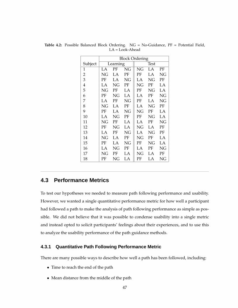
Table 4.2: Possible Balanced Block Ordering. NG = No-Guidance, PF = Potential Field,LA = Look-Ahead
Block OrderingSubject Learning Test1 LA PF NG NG LA PF2 NG LA PF PF LA NG3 PF LA NG LA NG PF4 LA NG PF NG PF LA5 NG PF LA PF NG LA6 PF NG LA LA PF NG7 LA PF NG PF LA NG8 NG LA PF LA NG PF9 PF LA NG NG PF LA10 LA NG PF PF NG LA11 NG PF LA LA PF NG12 PF NG LA NG LA PF13 LA PF NG LA NG PF14 NG LA PF NG PF LA15 PF LA NG PF NG LA16 LA NG PF LA PF NG17 NG PF LA NG LA PF18 PF NG LA PF LA NG
4.3 Performance Metrics
To test our hypotheses we needed to measure path following performance and usability.
However, we wanted a single quantitative performance metric for how well a participant
had followed a path to make the analysis of path following performance as simple as pos-
sible. We did not believe that it was possible to condense usability into a single metric
and instead opted to solicit participants’ feelings about their experiences, and to use this
to analyze the usability performance of the path guidance methods.
4.3.1 Quantitative Path Following Performance Metric
There are many possible ways to describe how well a path has been followed, including:
• Time to reach the end of the path
• Mean distance from the middle of the path
47
• Mean rate of change of the distance from the middle of the path
• Mean of the square of distance from the middle of the path.
• Frequency of leaving the path’s channel
• Smoothness of the trajectory
• Length of the traversed path compared to the path length
• Shape of traversed path compared to shape of the path being followed.
We wanted to keep our analysis as simple as possible and therefore wanted a single
quantitative path following metric. It is possible to use multiple measurements to rep-
resent path following performance, but this requires complicated multi-variate analysis
without necessarily clarifying the results.
After some careful consideration we decided that the Mean Square Error (MSE), where
the error is the distance of the vehicle from the middle of the path, was the most suitable
all-around path following performance metric for our needs. Equation 4.1 shows how the
MSE is computed, where On is the location of the vehicle at time n, and Opathn is the point
on the centerline of the path closest to point On at time n:
MSE =∑N−1
n=0 |On −Opathn|2
N· (4.1)
The MSE performance metric is inversely proportional to overall path following per-
formance; a low MSE score indicates better path following performance than a high MSE
score. However, it does not take into account the width of the path being followed.
We had originally envisioned an experimental task of following the path while try-
ing to stay within the extent of the path. In the pilot studies discussed in Section 4.6, we
found that with these instructions participants often cut corners, staying within the path
but moving away from the center of the path, adversely affecting their MSE score. In an at-
tempt to get participants to use a path following-strategy that would yield consistent, and
thus directly comparable, MSE scores, we augmented the experiment instructions on path
following to have a primary task of staying within the extent of the path, and a secondary
task of following the middle of the path closely as possible.
48
4.3.2 Subjective Evaluation Methods
While we were interested in learning which guidance method performed the ‘best’ accord-
ing to a numerical measurement, we were also interested in the usability of each guidance
method, which required us to inquire about users’ reactions to each guidance method.
We felt that the usability of each guidance method could be assessed by asking each
participant to evaluate three different subjective performance indicators:
1. Perceived degree of vehicle control
2. Perceived helpfulness of the provided guidance
3. Degree of pleasure afforded by the force feedback
Questions to address these three issues were presented to the participant via a dialog
box (Figure 4.3), following each block of thirty trials. These questions had to be answered
before the participant could move on to the next block of trials.
The session ended with a debriefing interview, the purpose of which was to solicit rele-
vant background information along with the participant’s impressions of his experiences.
The interview questions are included as Appendix C. The interview questions inquire
about experience with video games, driving and other force feedback devices. We also in-
quired about which guidance method participants liked the most, and if they felt that any
particular guidance method improved their performance. Other experiments conducted
by this research group have found anecdotal evidence that suggests a correlation between
performance with experimental tasks similar to ours and video gaming experience, hence
our interest in video gaming experience. The debriefing interview was audio-recorded for
later analysis.
4.4 Data Collected
We collected a variety of data over the course of an experiment session. Data about the
state of the simulation, such as the distance of the vehicle from the path, was collected at
60 Hz during every trial and saved to disk in a comma separated value (CSV) file. Par-
49
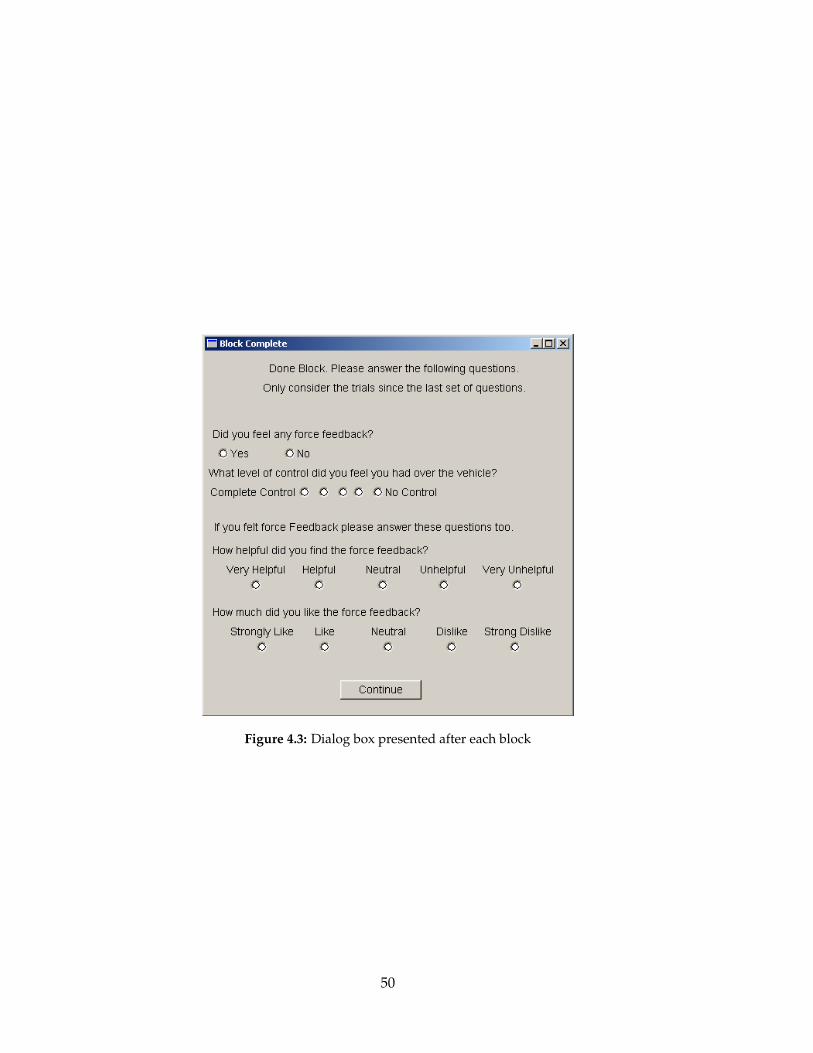
Figure 4.3: Dialog box presented after each block
50
ticipants were automatically asked questions after each block and the answers to these
questions were saved to a text file.
4.5 Procedure
To minimize possible distractions to the participants, the experiment was conducted in a
special acoustically insulated, windowless experiment room (the Imager lab experimenta-
tion facility), and lasted approximately one hour. The experiment room contained a flat-
screen LCD monitor on a table next to the haptic interface, and an adjustable office chair
faced the desk and monitor. The experiment consisted of four different stages: instruction,
familiarization, experiment, and interview.
Upon arrival, a participant was shown to the experiment room and given a waiver to
read and sign (see Appendix E). The participant was then seated in front of the computer
screen on which instructions for the experiment were displayed. The on-screen instruc-
tions inform the participant of experiment objective and what to expect; they also instruct
the participant to get comfortable and to be sure to check with the experimenter if, at any
time, questions arise (see Appendix B). Once the participant has read and understood the
instructions the experimenter begins the familiarization phase. The experimenter stays in
the room to observe the participant performing the familiarization trials and to answer any
questions. The full experiment of six blocks, each of thirty trials, starts once the participant
completes the familiarization phase, and both the participant and experimenter feel that
the participant is ready to continue.
The experimenter leaves the room to let the participant complete the full experiment
without further assistance. Initially, the screen contains a message telling the participant to
hit the space bar to start the first trial. A trial ends when the participant successfully nav-
igates to the end of the path, at which point the screen clears and the “Click on space bar
to continue” screen appears. The next trial does not begin until the space bar is pressed.
This process is repeated until the participant has completed the block of thirty trials and
then a dialog box (Figure 4.3) appears with questions for the participant regarding his ex-
periences over the previous block as described in Section 4.3.2. The whole process repeats
51
for the second block and so on, until the participant has completed all six blocks (180 tri-
als); at which point the participant has been instructed to retrieve the experimenter for the
debriefing interview.
The participant is told prior to the beginning of the debriefing interview that the inter-
view will be recorded for later analysis. The experimenter then conducts the interview and
records answers to the simpler questions, such as age, on a prepared form. Once the ques-
tioning part of the interview is over the audio recording is stopped and the experimenter
explains to the participant the purpose of the experiment and answers any questions the
participant may have about the experiment. At the end of this process the participant is
given an honorarium of $10.00 for his hour’s effort.
4.6 Pilot Studies
We performed two pilot studies before conducting the final experiment to verify both our
experimental process and our software. The first pilot (seven participants) suggested many
improvements and the second pilot (five participants) was more of a fine tuning before the
full experiment. Both pilots consisted of a familiarization phase followed by three blocks
of thirty trials each and were done less formally than was the final study (e.g. not in the
experiment room) with members or friends of our lab as participants.
The first pilot differed from the final experiment principally in the paths used. In the
pilot we used the paths: straight, curve and zigzag for low, medium and high complexity
levels (as opposed to the curve, bump, zigzag paths used in the final experiment); and
these paths were also twice as wide as the paths in the final version. We discovered in the
first pilot study that in general, these paths were too easy to follow. To address this issue
we made the paths narrower, and removed the straight path as the lowest complexity path
type because due to the knob centering force, it could be followed exactly without touching
the knob. A new path, bump, replaced the curve path as the medium complexity path and
the curve path became the low complexity path.
The first pilot study also identified some conflicts between our guidance methods,
quantitative metric and instructions. Our performance metric penalizes any path follow-
52
ing behavior that does not try to follow the center of the path, and some pilot participants
were cutting corners. We changed the experiment instructions tell the participants to try
stay on the path as well as to follow the center of the path. As a visual cue, the center of
the path was rendered as a thin, red line on top of the path extent.
Pilot Study Two was performed in the same manner as Pilot Study One, but with the
above noted changes implemented. After running Pilot Study Two and analyzing the data
from both pilot studies we noticed that there was a substantial learning effect as partici-
pants progressed through the study. We also noticed that the time to perform one trial was
much less than the thirty seconds we had budgeted for. With the extra time we had as a
result of this, we doubled the number of trials each participant would do as discussed in
Section 4.2.2.
53

Chapter 5
Experiment Results and Analysis
In this chapter we report our experiment results and their analysis. Section 5.1 describes
participant profiles, 5.2 our quantitative results and 5.3 our qualitative (subjective) results.
5.1 Experiment Participant Demographics
Our experimental design called for eighteen participants. We recruited participants via
Usenet posts, by using our group’s database of previous participants, and by word of
mouth. In total, we recruited twenty participants but only analyzed the data from eigh-
teen of these participants as two participants did not complete the experiment. One partic-
ipant left after the eighteen trial familiarization phase because she was too frustrated with
the difficulty of the task to continue. The other participant left after partially completing
the full experiment when she started to feel ill from either motion or VR (Virtual Reality)
sickness. The remaining eighteen participants completed the full experiment.
The first half of the post-experiment interview (Appendix C) was used to solicit rel-
evant demographic information about the participant. In addition to the standard age,
gender and handedness information, we were also interested in the participant’s driving,
video game and haptic interface background. Table 5.1 summarizes the results of the de-
mographic questions for the eighteen participants that successfully completed the study.
Thirteen participants reported playing video games, with eight of those reporting aver-
age playing times of at least one hour per week on average at the time of their participation
55
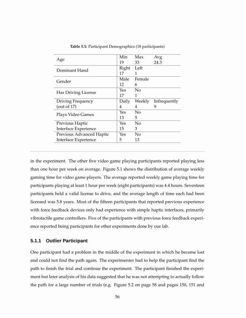
Table 5.1: Participant Demographics (18 participants)
Min Max AvgAge19 33 24.3Right LeftDominant Hand17 1Male FemaleGender12 6Yes NoHas Driving License17 1
Driving Frequency Daily Weekly Infrequently(out of 17) 4 4 9
Yes NoPlays Video Games13 5
Previous Haptic Yes NoInterface Experience 15 3Previous Advanced Haptic Yes NoInterface Experience 5 13
in the experiment. The other five video game playing participants reported playing less
than one hour per week on average. Figure 5.1 shows the distribution of average weekly
gaming time for video game players. The average reported weekly game playing time for
participants playing at least 1 hour per week (eight participants) was 4.4 hours. Seventeen
participants held a valid license to drive, and the average length of time each had been
licensed was 5.8 years. Most of the fifteen participants that reported previous experience
with force feedback devices only had experience with simple haptic interfaces, primarily
vibrotactile game controllers. Five of the participants with previous force feedback experi-
ence reported being participants for other experiments done by our lab.
5.1.1 Outlier Participant
One participant had a problem in the middle of the experiment in which he became lost
and could not find the path again. The experimenter had to help the participant find the
path to finish the trial and continue the experiment. The participant finished the experi-
ment but later analysis of his data suggested that he was not attempting to actually follow
the path for a large number of trials (e.g. Figure 5.2 on page 58 and pages 150, 151 and
56
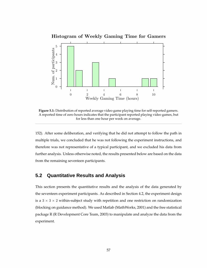
Histogram of Weekly Gaming Time for Gamers
Weekly Gaming Time (hours)
Num
. of
par
tici
pan
ts
0
1
2
3
4
5
0 2 4 6 8 10
Figure 5.1: Distribution of reported average video game playing time for self-reported gamers.A reported time of zero hours indicates that the participant reported playing video games, but
for less than one hour per week on average.
152). After some deliberation, and verifying that he did not attempt to follow the path in
multiple trials, we concluded that he was not following the experiment instructions, and
therefore was not representative of a typical participant, and we excluded his data from
further analysis. Unless otherwise noted, the results presented below are based on the data
from the remaining seventeen participants.
5.2 Quantitative Results and Analysis
This section presents the quantitative results and the analysis of the data generated by
the seventeen experiment participants. As described in Section 4.2, the experiment design
is a 3 × 3 × 2 within-subject study with repetition and one restriction on randomization
(blocking on guidance method). We used Matlab (MathWorks, 2001) and the free statistical
package R (R Development Core Team, 2003) to manipulate and analyze the data from the
experiment.
57
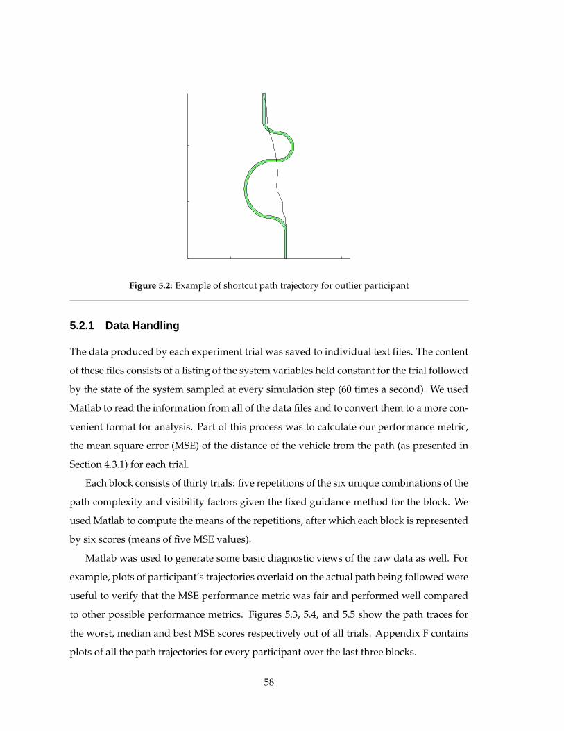
Figure 5.2: Example of shortcut path trajectory for outlier participant
5.2.1 Data Handling
The data produced by each experiment trial was saved to individual text files. The content
of these files consists of a listing of the system variables held constant for the trial followed
by the state of the system sampled at every simulation step (60 times a second). We used
Matlab to read the information from all of the data files and to convert them to a more con-
venient format for analysis. Part of this process was to calculate our performance metric,
the mean square error (MSE) of the distance of the vehicle from the path (as presented in
Section 4.3.1) for each trial.
Each block consists of thirty trials: five repetitions of the six unique combinations of the
path complexity and visibility factors given the fixed guidance method for the block. We
used Matlab to compute the means of the repetitions, after which each block is represented
by six scores (means of five MSE values).
Matlab was used to generate some basic diagnostic views of the raw data as well. For
example, plots of participant’s trajectories overlaid on the actual path being followed were
useful to verify that the MSE performance metric was fair and performed well compared
to other possible performance metrics. Figures 5.3, 5.4, and 5.5 show the path traces for
the worst, median and best MSE scores respectively out of all trials. Appendix F contains
plots of all the path trajectories for every participant over the last three blocks.
58
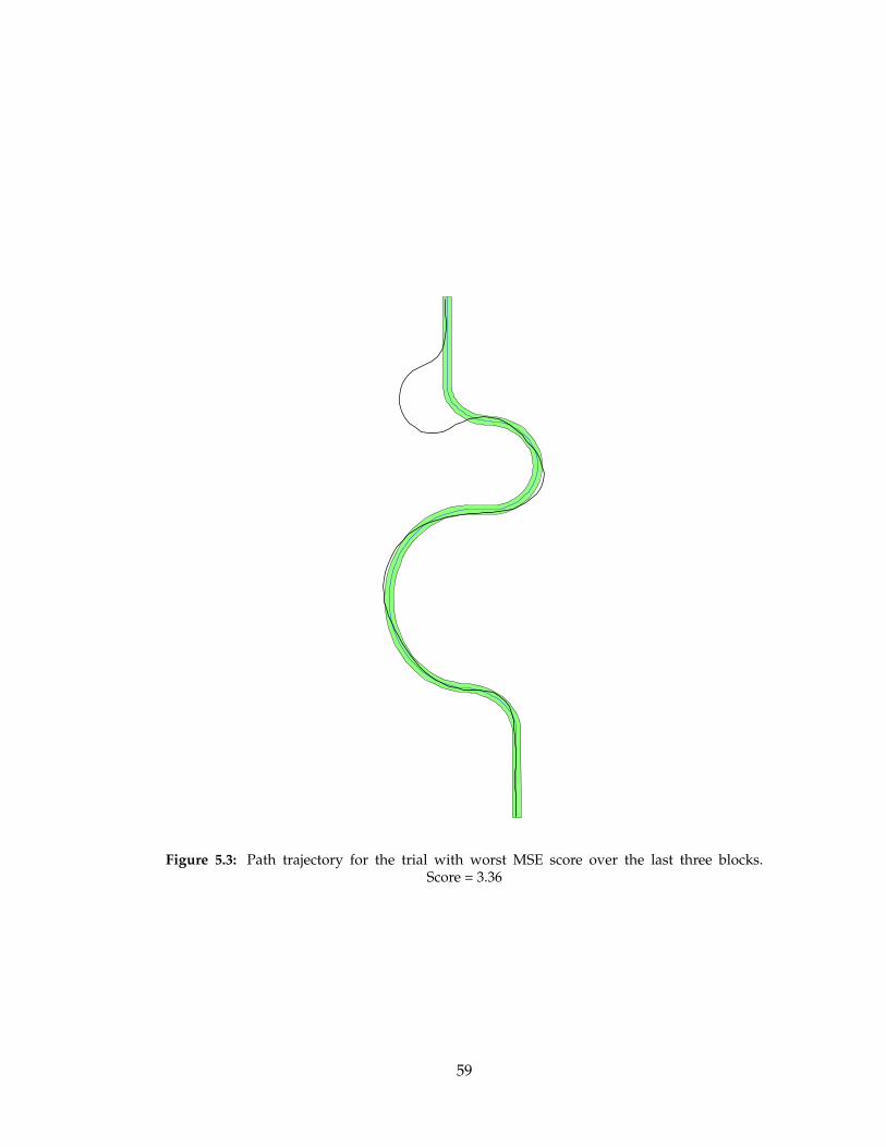
Figure 5.3: Path trajectory for the trial with worst MSE score over the last three blocks.Score = 3.36
59
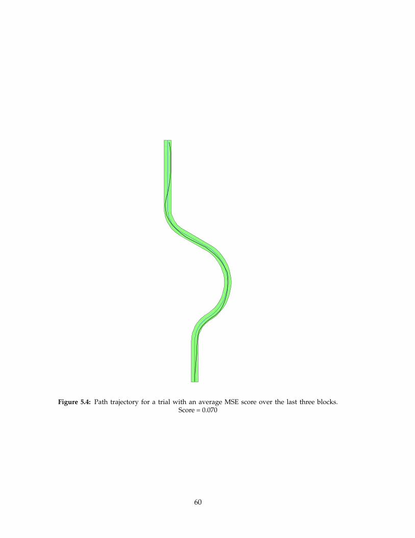
Figure 5.4: Path trajectory for a trial with an average MSE score over the last three blocks.Score = 0.070
60
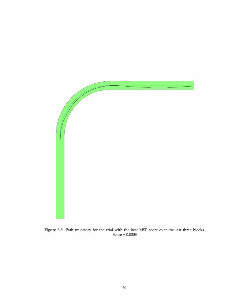
Figure 5.5: Path trajectory for the trial with the best MSE score over the last three blocks.Score = 0.0008
61
The data needed for a complete statistical analysis was exported from Matlab to a
comma separated value (CSV) file and imported into R for analysis. The following data
was exported: participant number, guidance method level, path complexity level, visibility
level, MSE (performance metric), and block number. R makes it easy to perform complex
ANOVA analyses, such as the one we needed to do.
5.2.2 Statistical Analysis
We designed and executed a 3× 3× 2 repeated measures experiment with balanced block-
ing on the three different levels of the guidance method factor. We analyzed the final three
blocks of the experiment; the data from the first three blocks was treated as a learning
phase and was not analyzed. The box-plot shown in Figure 5.6 on the next page shows the
scores for all six experimental blocks and suggests that the performance improves consid-
erably over the first three blocks and is consistent for the final three blocks. The variability
of scores decreases rapidly over the first two blocks. We believe that it safe to say that
any learning effects have been significantly reduced by the final three blocks. Satisfied
that there was minimal learning happening over the final three experimental blocks, we
performed a within-subject ANOVA, using R to test the effect, if any, of our independent
variables on our performance metric.
We performed a full within-subject ANOVA, after averaging out the repetitions, to
test for an effect of our three independent variables on the MSE performance metric (the
dependent variable). This procedure is accomplished in R by the aov() function which is
discussed in Appendix D. Table 5.2 shows the results of the within-subject ANOVA. It is
evident from the ANOVA table that all of the main effects are significant at the p < 0.05
level, but there are no significant interaction effects.
The significant results from the ANOVA indicate that there are main effects but does
not indicate the relative effects for the different levels of the independent variables if they
have more than two levels. We performed a post-hoc, pairwise comparison (with the Holm
p-value adjustment) between the levels of the guidance method and the path complexity
factors to see where the difference between levels are. The results of the pairwise compar-
isons between levels of the guidance method factor are presented in Table 5.4 on page 65
62
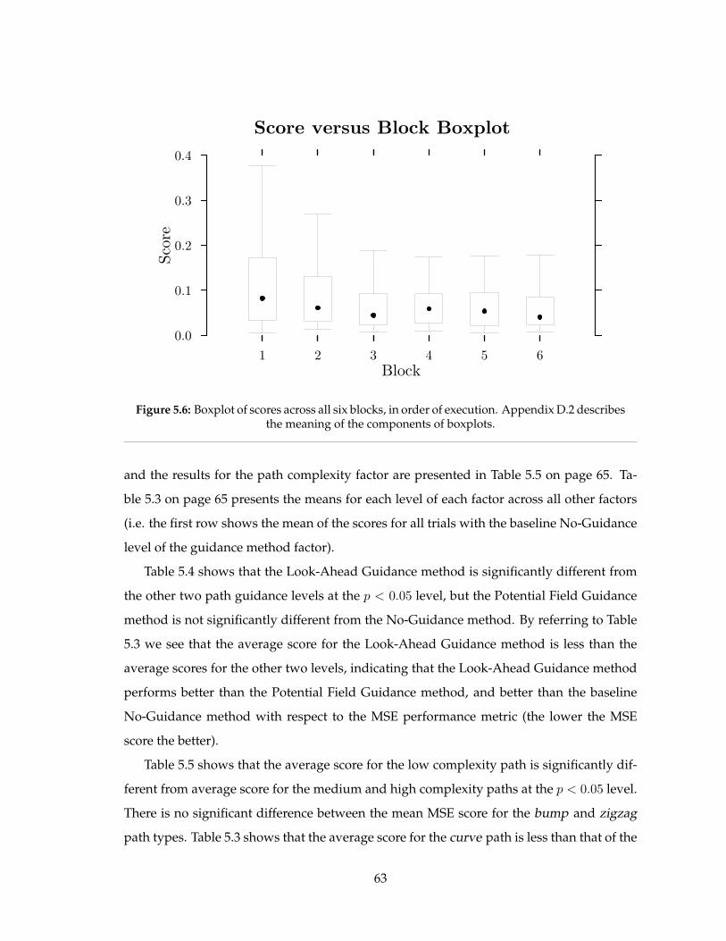
Score versus Block Boxplot
Block
Score
0.0
0.1
0.2
0.3
0.4
1 2 3 4 5 6
Figure 5.6: Boxplot of scores across all six blocks, in order of execution. Appendix D.2 describesthe meaning of the components of boxplots.
and the results for the path complexity factor are presented in Table 5.5 on page 65. Ta-
ble 5.3 on page 65 presents the means for each level of each factor across all other factors
(i.e. the first row shows the mean of the scores for all trials with the baseline No-Guidance
level of the guidance method factor).
Table 5.4 shows that the Look-Ahead Guidance method is significantly different from
the other two path guidance levels at the p < 0.05 level, but the Potential Field Guidance
method is not significantly different from the No-Guidance method. By referring to Table
5.3 we see that the average score for the Look-Ahead Guidance method is less than the
average scores for the other two levels, indicating that the Look-Ahead Guidance method
performs better than the Potential Field Guidance method, and better than the baseline
No-Guidance method with respect to the MSE performance metric (the lower the MSE
score the better).
Table 5.5 shows that the average score for the low complexity path is significantly dif-
ferent from average score for the medium and high complexity paths at the p < 0.05 level.
There is no significant difference between the mean MSE score for the bump and zigzag
path types. Table 5.3 shows that the average score for the curve path is less than that of the
63
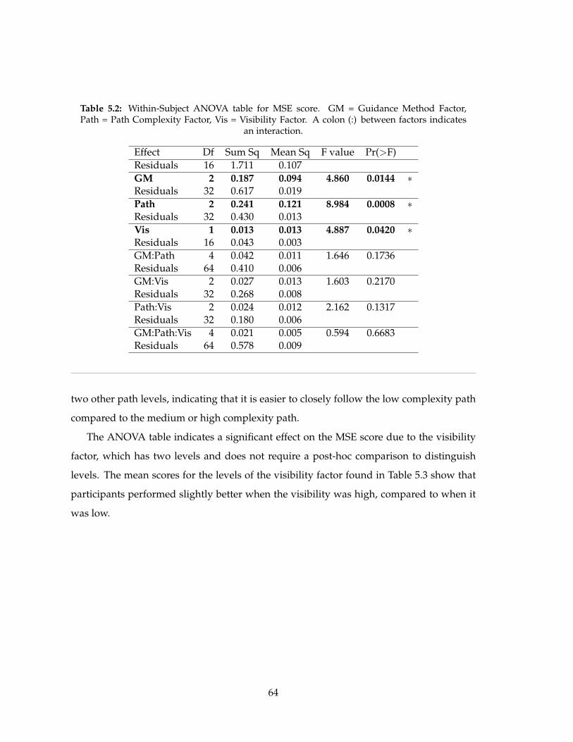
Table 5.2: Within-Subject ANOVA table for MSE score. GM = Guidance Method Factor,Path = Path Complexity Factor, Vis = Visibility Factor. A colon (:) between factors indicates
an interaction.
Effect Df Sum Sq Mean Sq F value Pr(>F)Residuals 16 1.711 0.107GM 2 0.187 0.094 4.860 0.0144 ∗Residuals 32 0.617 0.019Path 2 0.241 0.121 8.984 0.0008 ∗Residuals 32 0.430 0.013Vis 1 0.013 0.013 4.887 0.0420 ∗Residuals 16 0.043 0.003GM:Path 4 0.042 0.011 1.646 0.1736Residuals 64 0.410 0.006GM:Vis 2 0.027 0.013 1.603 0.2170Residuals 32 0.268 0.008Path:Vis 2 0.024 0.012 2.162 0.1317Residuals 32 0.180 0.006GM:Path:Vis 4 0.021 0.005 0.594 0.6683Residuals 64 0.578 0.009
two other path levels, indicating that it is easier to closely follow the low complexity path
compared to the medium or high complexity path.
The ANOVA table indicates a significant effect on the MSE score due to the visibility
factor, which has two levels and does not require a post-hoc comparison to distinguish
levels. The mean scores for the levels of the visibility factor found in Table 5.3 show that
participants performed slightly better when the visibility was high, compared to when it
was low.
64
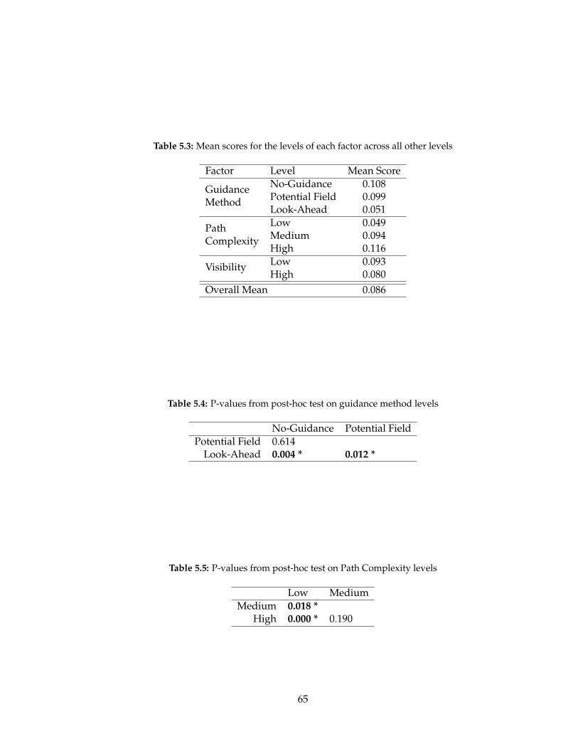
Table 5.3: Mean scores for the levels of each factor across all other levels
Factor Level Mean ScoreNo-Guidance 0.108GuidancePotential Field 0.099MethodLook-Ahead 0.051Low 0.049PathMedium 0.094ComplexityHigh 0.116Low 0.093VisibilityHigh 0.080
Overall Mean 0.086
Table 5.4: P-values from post-hoc test on guidance method levels
No-Guidance Potential FieldPotential Field 0.614
Look-Ahead 0.004 * 0.012 *
Table 5.5: P-values from post-hoc test on Path Complexity levels
Low MediumMedium 0.018 *
High 0.000 * 0.190
65
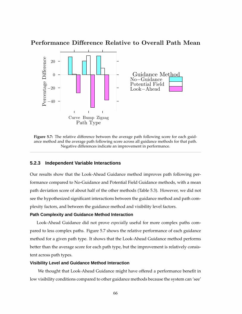
Performance Difference Relative to Overall Path Mean
Path Type
Per
centa
ge
Diffe
rence
−40
−20
0
20
Curve Bump Zigzag
Guidance MethodNo−GuidancePotential FieldLook−Ahead
Figure 5.7: The relative difference between the average path following score for each guid-ance method and the average path following score across all guidance methods for that path.
Negative differences indicate an improvement in performance.
5.2.3 Independent Variable Interactions
Our results show that the Look-Ahead Guidance method improves path following per-
formance compared to No-Guidance and Potential Field Guidance methods, with a mean
path deviation score of about half of the other methods (Table 5.3). However, we did not
see the hypothesized significant interactions between the guidance method and path com-
plexity factors, and between the guidance method and visibility level factors.
Path Complexity and Guidance Method Interaction
Look-Ahead Guidance did not prove especially useful for more complex paths com-
pared to less complex paths. Figure 5.7 shows the relative performance of each guidance
method for a given path type. It shows that the Look-Ahead Guidance method performs
better than the average score for each path type, but the improvement is relatively consis-
tent across path types.
Visibility Level and Guidance Method Interaction
We thought that Look-Ahead Guidance might have offered a performance benefit in
low visibility conditions compared to other guidance methods because the system can ‘see’
66
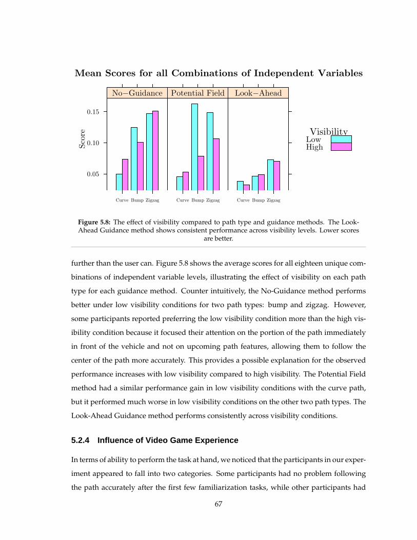
Mean Scores for all Combinations of Independent VariablesSco
re
0.05
0.10
0.15
Curve Bump Zigzag
No−Guidance
Curve Bump Zigzag
Potential Field
Curve Bump Zigzag
Look−Ahead
VisibilityLowHigh
Figure 5.8: The effect of visibility compared to path type and guidance methods. The Look-Ahead Guidance method shows consistent performance across visibility levels. Lower scores
are better.
further than the user can. Figure 5.8 shows the average scores for all eighteen unique com-
binations of independent variable levels, illustrating the effect of visibility on each path
type for each guidance method. Counter intuitively, the No-Guidance method performs
better under low visibility conditions for two path types: bump and zigzag. However,
some participants reported preferring the low visibility condition more than the high vis-
ibility condition because it focused their attention on the portion of the path immediately
in front of the vehicle and not on upcoming path features, allowing them to follow the
center of the path more accurately. This provides a possible explanation for the observed
performance increases with low visibility compared to high visibility. The Potential Field
method had a similar performance gain in low visibility conditions with the curve path,
but it performed much worse in low visibility conditions on the other two path types. The
Look-Ahead Guidance method performs consistently across visibility conditions.
5.2.4 Influence of Video Game Experience
In terms of ability to perform the task at hand, we noticed that the participants in our exper-
iment appeared to fall into two categories. Some participants had no problem following
the path accurately after the first few familiarization tasks, while other participants had
67

Average Score For Each Block Given Game Playing Status
Block
Aver
age
Sco
re
0.05
0.10
0.15
0.20
0.25
0.30
1 2 3 4 5 6
Plays Video Gamesnoyes
Figure 5.9: Mean score across all conditions for each block given gaming experience
difficulty throughout the primary familiarization phase and generally performed worse
than the other group of participants. An extreme example of this is the participant who
left after the familiarization phase because of frustration with the task. While running
the experiment we hypothesized that this difference between participants may have been
related to video game experience, based on past experiences in our research group.
Figure 5.9 shows the performance of gamers and non-gamers according to block num-
ber, illustrating how performance changes over time. Both groups tend to improve over
time, but the improvement is more pronounced in non-gamers than it is in gamers with
the exception of the last block. This suggests that non-gamers improve more than gamers
do over time, although still not reaching the performance level of gamers. The poor perfor-
mance of non-gamers in the last block possibly suggests that they become fatigued and/or
disinterested in the experiment by the last block.
Figure 5.10 on the next page shows individual participant scores in boxplot form and
are shaded according to game playing status. The vertical line in the figure indicates the
mean score across all participants and all conditions. The game players tend to have lower
(better) scores than non-game players with an average score of 0.13 for non-gamers and
0.067 for gamers, but there is considerable overlap. Figure 5.11 shows boxplots for the
68
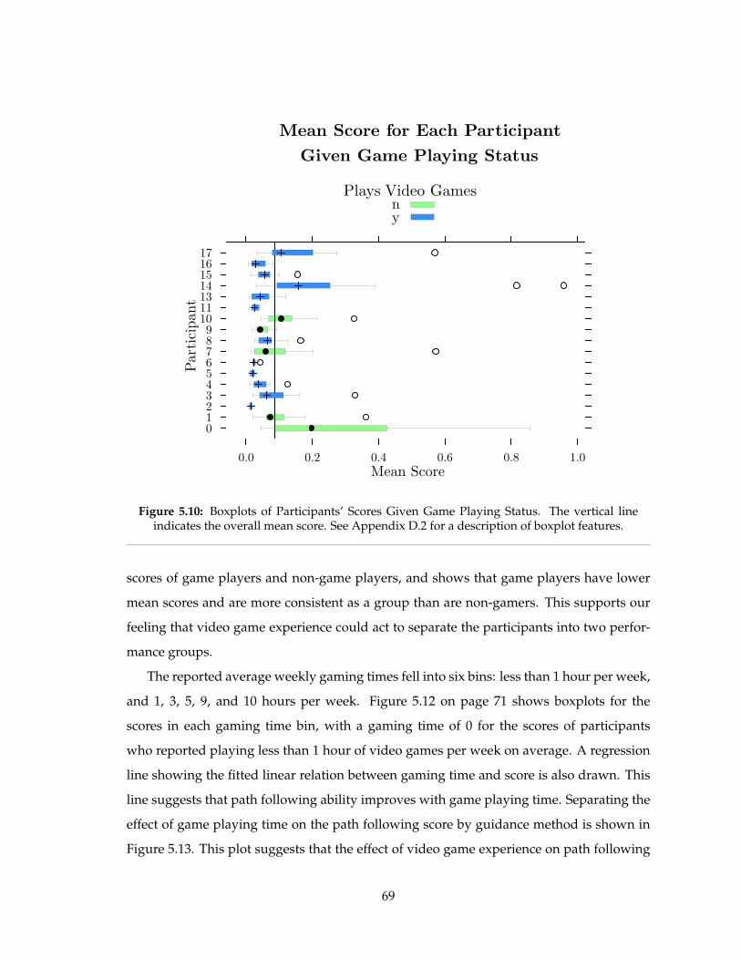
Mean Score for Each Participant
Given Game Playing Status
Mean Score
Part
icip
ant
0 1 2 3 4 5 6 7 8 9
10 11 13 14 15 16 17
0.0 0.2 0.4 0.6 0.8 1.0
Plays Video Games n y
Figure 5.10: Boxplots of Participants’ Scores Given Game Playing Status. The vertical lineindicates the overall mean score. See Appendix D.2 for a description of boxplot features.
scores of game players and non-game players, and shows that game players have lower
mean scores and are more consistent as a group than are non-gamers. This supports our
feeling that video game experience could act to separate the participants into two perfor-
mance groups.
The reported average weekly gaming times fell into six bins: less than 1 hour per week,
and 1, 3, 5, 9, and 10 hours per week. Figure 5.12 on page 71 shows boxplots for the
scores in each gaming time bin, with a gaming time of 0 for the scores of participants
who reported playing less than 1 hour of video games per week on average. A regression
line showing the fitted linear relation between gaming time and score is also drawn. This
line suggests that path following ability improves with game playing time. Separating the
effect of game playing time on the path following score by guidance method is shown in
Figure 5.13. This plot suggests that the effect of video game experience on path following
69

Plays Video Games
Sco
re
0.0
0.2
0.4
0.6
0.8
1.0
n y
(a) Outliers Shown
Plays Video GamesSco
re
0.00
0.05
0.10
0.15
0.20
0.25
n y
(b) Zoomed (OutliersNot Shown)
Figure 5.11: Boxplots of participants’ scores given game playing status. Boxplot componentsare described in Appendix D.2
performance is lower with Look-Ahead Guidance than with the other guidance methods.
70
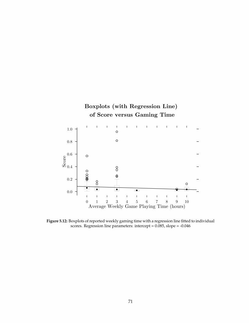
Boxplots (with Regression Line)
of Score versus Gaming Time
Average Weekly Game Playing Time (hours)
Sco
re
0.0
0.2
0.4
0.6
0.8
1.0
0 1 2 3 4 5 6 7 8 9 10
Figure 5.12: Boxplots of reported weekly gaming time with a regression line fitted to individualscores. Regression line parameters: intercept = 0.085, slope = -0.046
71
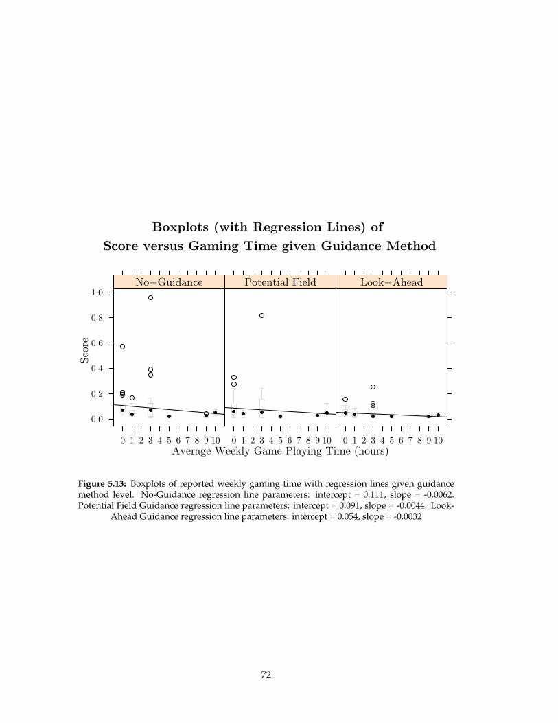
Boxplots (with Regression Lines) of
Score versus Gaming Time given Guidance Method
Average Weekly Game Playing Time (hours)
Sco
re
0.0
0.2
0.4
0.6
0.8
1.0
0 1 2 3 4 5 6 7 8 9 10
No−Guidance
0 1 2 3 4 5 6 7 8 9 10
Potential Field
0 1 2 3 4 5 6 7 8 9 10
Look−Ahead
Figure 5.13: Boxplots of reported weekly gaming time with regression lines given guidancemethod level. No-Guidance regression line parameters: intercept = 0.111, slope = -0.0062.Potential Field Guidance regression line parameters: intercept = 0.091, slope = -0.0044. Look-
Ahead Guidance regression line parameters: intercept = 0.054, slope = -0.0032
72
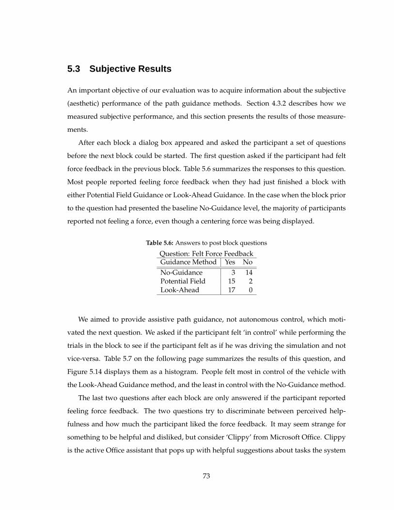
5.3 Subjective Results
An important objective of our evaluation was to acquire information about the subjective
(aesthetic) performance of the path guidance methods. Section 4.3.2 describes how we
measured subjective performance, and this section presents the results of those measure-
ments.
After each block a dialog box appeared and asked the participant a set of questions
before the next block could be started. The first question asked if the participant had felt
force feedback in the previous block. Table 5.6 summarizes the responses to this question.
Most people reported feeling force feedback when they had just finished a block with
either Potential Field Guidance or Look-Ahead Guidance. In the case when the block prior
to the question had presented the baseline No-Guidance level, the majority of participants
reported not feeling a force, even though a centering force was being displayed.
Table 5.6: Answers to post block questions
Question: Felt Force FeedbackGuidance Method Yes NoNo-Guidance 3 14Potential Field 15 2Look-Ahead 17 0
We aimed to provide assistive path guidance, not autonomous control, which moti-
vated the next question. We asked if the participant felt ‘in control’ while performing the
trials in the block to see if the participant felt as if he was driving the simulation and not
vice-versa. Table 5.7 on the following page summarizes the results of this question, and
Figure 5.14 displays them as a histogram. People felt most in control of the vehicle with
the Look-Ahead Guidance method, and the least in control with the No-Guidance method.
The last two questions after each block are only answered if the participant reported
feeling force feedback. The two questions try to discriminate between perceived help-
fulness and how much the participant liked the force feedback. It may seem strange for
something to be helpful and disliked, but consider ‘Clippy’ from Microsoft Office. Clippy
is the active Office assistant that pops up with helpful suggestions about tasks the system
73
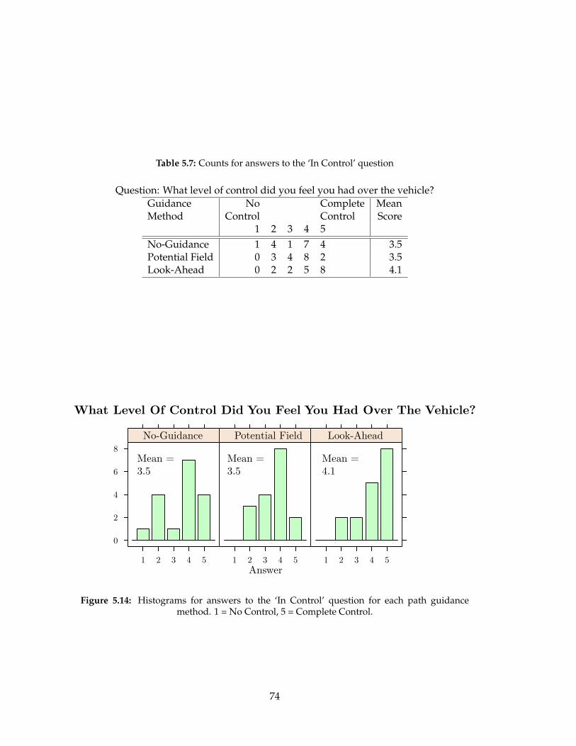
Table 5.7: Counts for answers to the ‘In Control’ question
Question: What level of control did you feel you had over the vehicle?Guidance No Complete MeanMethod Control Control Score
1 2 3 4 5No-Guidance 1 4 1 7 4 3.5Potential Field 0 3 4 8 2 3.5Look-Ahead 0 2 2 5 8 4.1
What Level Of Control Did You Feel You Had Over The Vehicle?
Answer
0
2
4
6
8
1 2 3 4 5
No-Guidance
1 2 3 4 5
Potential Field
1 2 3 4 5
Look-Ahead
Mean =
3.5
Mean =
3.5
Mean =
4.1
Figure 5.14: Histograms for answers to the ‘In Control’ question for each path guidancemethod. 1 = No Control, 5 = Complete Control.
74
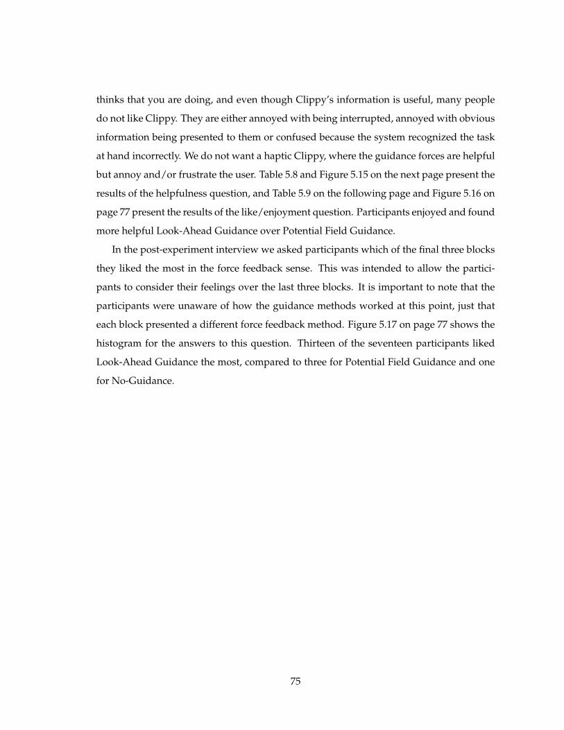
thinks that you are doing, and even though Clippy’s information is useful, many people
do not like Clippy. They are either annoyed with being interrupted, annoyed with obvious
information being presented to them or confused because the system recognized the task
at hand incorrectly. We do not want a haptic Clippy, where the guidance forces are helpful
but annoy and/or frustrate the user. Table 5.8 and Figure 5.15 on the next page present the
results of the helpfulness question, and Table 5.9 on the following page and Figure 5.16 on
page 77 present the results of the like/enjoyment question. Participants enjoyed and found
more helpful Look-Ahead Guidance over Potential Field Guidance.
In the post-experiment interview we asked participants which of the final three blocks
they liked the most in the force feedback sense. This was intended to allow the partici-
pants to consider their feelings over the last three blocks. It is important to note that the
participants were unaware of how the guidance methods worked at this point, just that
each block presented a different force feedback method. Figure 5.17 on page 77 shows the
histogram for the answers to this question. Thirteen of the seventeen participants liked
Look-Ahead Guidance the most, compared to three for Potential Field Guidance and one
for No-Guidance.
75
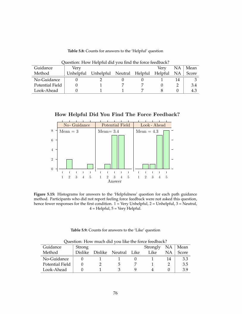
Table 5.8: Counts for answers to the ‘Helpful’ question
Question: How Helpful did you find the force feedback?Guidance Very Very NA MeanMethod Unhelpful Unhelpful Neutral Helpful Helpful NA ScoreNo-Guidance 0 2 0 0 1 14 3Potential Field 0 1 7 7 0 2 3.4Look-Ahead 0 1 1 7 8 0 4.3
How Helpful Did You Find The Force Feedback?
Answer
0
2
4
6
8
1 2 3 4 5
No- Guidance
1 2 3 4 5
Potential Field
1 2 3 4 5
Look - Ahead
Mean = 3 Mean= 3.4 Mean = 4.3
Figure 5.15: Histograms for answers to the ‘Helpfulness’ question for each path guidancemethod. Participants who did not report feeling force feedback were not asked this question,hence fewer responses for the first condition. 1 = Very Unhelpful, 2 = Unhelpful, 3 = Neutral,
4 = Helpful, 5 = Very Helpful.
Table 5.9: Counts for answers to the ‘Like’ question
Question: How much did you like the force feedback?Guidance Strong Strongly NA MeanMethod Dislike Dislike Neutral Like Like NA ScoreNo-Guidance 0 1 1 0 1 14 3.3Potential Field 0 2 5 7 1 2 3.5Look-Ahead 0 1 3 9 4 0 3.9
76
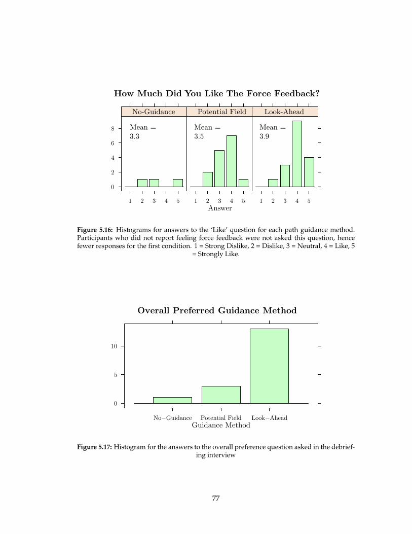
How Much Did You Like The Force Feedback?
Answer
0
2
4
6
8
1 2 3 4 5
No-Guidance
1 2 3 4 5
Potential Field
1 2 3 4 5
Look-Ahead
Mean =
3.3
Mean =
3.5
Mean =
3.9
Figure 5.16: Histograms for answers to the ‘Like’ question for each path guidance method.Participants who did not report feeling force feedback were not asked this question, hencefewer responses for the first condition. 1 = Strong Dislike, 2 = Dislike, 3 = Neutral, 4 = Like, 5
= Strongly Like.
Overall Preferred Guidance Method
Guidance Method
0
5
10
No−Guidance Potential Field Look−Ahead
Figure 5.17: Histogram for the answers to the overall preference question asked in the debrief-ing interview
77

Chapter 6
Discussion
In this Chapter we discuss issues and insights from the previous three Chapters about the
implementation, evaluation and results of our experiment.
6.1 Results and our Hypotheses
In this Section we present a discussion about what we learned about our hypotheses (Sec-
tion 4.1) given the results we presented in the previous Chapter.
6.1.1 Quantitative Performance of Look-Ahead Guidance
We hypothesized that Look-Ahead Guidance would exhibit performance benefits com-
pared to No-Guidance, our baseline, and to our alternative haptic method, Potential Field
Guidance. The results we present in Section 5.2 verify that Look-Ahead Guidance provides
a significant performance benefit compared to the other guidance methods across the set
of independent variables we varied; with respect to our chosen performance metric, the
mean square error of lateral deviation from the center of the path. Our best attempt at
Potential Field Guidance for our haptic interface did not offer a significant performance
benefit compared to No-Guidance, suggesting that the specific mechanism and implemen-
tation of haptic guidance are crucial in providing a performance benefit. The lack of signif-
icant interactions in the ANOVA analysis (Table 5.2) suggests that Look-Ahead Guidance
offers a performance benefit, compared to the other guidance methods, across a range of
79
path complexities and visibility levels — it is not limited to offering performance benefits
for a small subset of path following tasks.
However, there are some details related to our implementation and evaluation method-
ologies that should be taken into account before concluding that Look-Ahead Guidance is
an improvement over all potential field guidance methods, or across all path complexi-
ties and visibility levels. These details include Potential Field Guidance implementation
choices and the choice of our quantitative performance metric.
6.1.1.1 Design and Implementation of Guidance Methods
As our primary focus, Look-Ahead Guidance received more development time than did
Potential Field Guidance. A potential field guidance method is easy to implement using
a two DoF interface for a two DoF task, such as tracing a path with a pen-like interface,
but potential field guidance for an under-actuated task, such as our driving task, is not as
straightforward. There are multiple possible implementations that could be called a ‘po-
tential field’ method, and we implemented as close to a direct 1D analog of the 2D path
tracing potential field method we could devise (Section 3.2.4) that had a reasonable level
of usability. However, we used the same desired steering angle control system for the Po-
tential Field Guidance method as we did for the Look-Ahead Guidance method (Section
3.2.2), which is awkward because the idea of a desired steering angle seems to violate the
‘spirit’ of potential field methods. However, time constraints prevented us from devel-
oping an alternative control system especially for our Potential Field Guidance method.
We are satisfied that our implementation is representative of potential field methods in
general, but there are many possible ways to implement such methods and the one we
have chosen to use may not be the absolute best. Vector fields are a possible alternative
implementation style to base potential field guidance upon that may be an improvement
compared to our style.
6.1.1.2 Quantitative Performance Metric and Experiment Task Interaction
The choice of how to measure path following performance is a critical component of the
evaluation of any path following experiment. We chose to use the mean square error of the
80
deviation from the center of the path as discussed in Section 4.3.1. There were trade-offs
associated with this choice, and slight modifications to the design of our experiment were
required to accommodate this choice.
We wanted the participant to stay inside a path while following it from beginning to
end, but to be fair to our chosen performance metric we were required to add the secondary
task of following the center of the path as closely as possible as well. Following the center
of the path is more difficult than merely staying within the extent of the path, and this may
have influenced participants’ path following strategies. Participants attempting to follow
the center of the path as closely as possible will probably focus on the path just in front of
the vehicle, limiting the perception of upcoming path features which could influence high
level path following strategies. Participants only trying to stay within the extent of the
path have more leeway and can afford to move their focus further away from the vehicle
than can the center following participants, and therefore are more likely to use upcoming
path features in their path following strategy. It is possible this speculated focus-point
artifact may have contributed to the observed consistent performance benefit of the Look-
Ahead Guidance method because it may have been always looking further ahead than
the participants were, signaling path changes haptically before the participant visually
recognized them.
6.1.2 Guidance Methods and Path Complexity
We evaluated path following performance across three different path complexities: low
(curve), medium (bump) and high (zigzag). We used an ad-hoc method to create paths
for each of these categories, and our statistical results suggest that only two different path
complexities existed. Table 5.5 on page 65 shows that there was a significant performance
difference between the low complexity path and both the medium and high complexity
paths, but there was no significant performance difference between the medium and high
complexity paths, suggesting that the complexities of these two paths were at a similar
level.
Figure 5.7 on page 66 shows that Look-Ahead Guidance offers a consistent perfor-
mance benefit compared to the average performance for each path type. Similarly, No-
81
Guidance performs consistently worse than average across all three path complexities. The
performance of Potential Field Guidance varies considerably across path complexities, but
this could be due to its poor performance in the low visibility condition with the medium
and high complexity paths as evident in Figure 5.8 on page 67.
6.1.3 Guidance Methods and Visibility
Our results show that there is a statistically significant difference in performance between
low and high visibility conditions (Table 5.2), but the interaction between guidance method
and visibility is not significant. We had speculated that Look-Ahead Guidance would per-
form better in low visibility conditions compared to the other guidance methods because it
‘sees’ through the darkness of the low visibility condition, which the other methods do not
do. Figure 5.8 shows that Look-Ahead Guidance does perform better than the other guid-
ance methods in low visibility conditions, but does not itself exhibit a large performance
difference between visibility conditions. The same cannot be said for the other guidance
methods.
Both No-Guidance and Potential Field Guidance exhibit a counter-intuitive perfor-
mance benefit in low visibility conditions with the low complexity curve path. However,
these methods do tend to perform worse under the low visibility condition for the more
complex path types. One possible explanation for this is mentioned in Section 5.2.3. The
low visibility condition forced participants to focus on the path closer to the vehicle than
they normally would. A narrowed focus helps users to follow the center of the path in
simple situations, such as the low complexity curve path with a single corner, but has
the potential to adversely impact higher-level path planning required to accurately follow
more complex, multi-cornered paths such as bump and zigzag. One possible explanation
for why this performance trend is not apparent with Look-Ahead Guidance is that it is
always looking further ahead than the participant is, and so low visibility does not have
any power to impact performance. Perhaps this would not be the case if participants were
not attempting to follow the center of the path in addition to staying within its extent.
82
6.1.4 Subjective Performance of the Guidance Methods
Our subjective evaluation methods sufficiently addressed the issues in which we were in-
terested: perceived level of control, the preferred guidance method and any discrepancy
between perceived helpfulness and aesthetic preference. Look-Ahead Guidance gave par-
ticipants a better sense of control over the vehicle compared to the other guidance methods,
an important characteristic for a usable guidance method. A guidance method could force
the user to follow a path exactly, but if the user did not feel that he had control there is a
good chance that the guidance method would not be accepted. When participants reported
feeling force feedback, Look-Ahead Guidance was reported to be more helpful and liked
more than the other guidance methods. This consistency between like and helpfulness is
important, as it indicates that Look-Ahead Guidance is not the haptic equivalent of Clippy.
The majority of participants reported preferring the block corresponding to Look-Ahead
Guidance during the debriefing interview. Participants were considering individual blocks
for the subjective measurements taken before the interview, yet even when concurrently
considering the final three blocks in the interview thirteen of seventeen participants (76%)
preferred Look-Ahead Guidance. While these results are encouraging, we consider that
they could have been reinforced with more detailed subjective evaluation methods.
The post experiment interview was used to solicit participants’ feelings about the ex-
periment as a whole, to complement the questions asked automatically after each experi-
mental block. One thing that we did not ask, but wish that we had, concerned which of
the last three blocks a participant liked the least, in addition to asking which block they
liked the most. We should also have attempted to elicit more detailed descriptions of why
participants selected the block that they did as their favourite. Most answers were very
short and not particularly informative in the structured component of the debriefing inter-
view. The occasional participant would provide more interesting answers but this usually
happened in the more free-form Q & A session, after the audio recording was stopped. The
experimenter stopped the audio recorder at the end of the interview questions before they
explained the purpose of the experiment to save recording media. This explanation of the
study occasionally prompted a discussion about the details of the system, and here the
participant would discuss his preferences and interpretations with more detail than he did
83
previously. These discussions were only captured in note form by the experimenter and
some potentially interesting discussion details were lost.
6.2 General Observations
In this section we develop general observations about our experimental methodology and
results not directly related to our hypotheses.
6.2.1 Issues with Physical Interaction and Real World Similarity
The perceived similarity between the experimental task and driving may have caused
some interaction problems and influenced learnability. We purposely made the experi-
mental task similar to driving in an attempt to reduce the learning curve compared to
more abstract tasks. This was desirable because our goal was to have a one hour long
experiment per participant, and we did not want to spend too much time familiarizing
participants with the task. However, the difference between the final implementation of
our task and driving in the real world may have been too significant for successful task
transfer.
The physical characteristics of our control knob offers a very different interaction style
than what one would have with a full-sized steering wheel. Interaction with our control
knob is performed with one arm and primarily involves wrist and finger motions, with
some small elbow rotations. A steering wheel, on the other hand, is typically controlled
with shoulder and elbow rotations from both arms. An advantage of a full sized steering
wheel is that small movements of the wheel engage similar motor units as do those of
large wheel movements. In contrast, the typical grasp of our device facilitated small knob
movements, and large movements involved significantly different motor units, requiring
the user to release the knob and reposition his fingers on the knob, similar to the way one
lifts and ‘scrolls’ the mouse on reaching the edge of the mouse pad.
Releasing the control knob of our haptic interface has a number of potential pitfalls.
One is that a spring centering force is being applied to the knob at all times, and as the
knob is released there is a force trying to center it. This can cause the knob to move in a
84
counter-productive direction before the user resumes grasping the knob. Once the desired
large motion has been completed the user must release the knob again to return to the
starting knob position; the problem compounds itself. We were unaware of this potential
problem during development because, being familiar with the interface, we could control
the vehicle well without releasing the knob; and it was not identified as a problem during
the pilot studies.
This knob interaction issue combined with the deliberate absence of user control over
vehicle velocity contributed to a significant difference between our experimental task and
driving. We suspect that this difference had an impact on the time required to become
proficient at interacting with our experimental system. However, our results do suggest
that learning had stabilized by our second set of blocks, which we base our analysis on.
6.2.2 Explicitness of Experiment Instructions
Upon reflection, the instructions presented to the participants could be improved. The
problems associated with interacting with a small control knob discussed in Section 6.2.1
may have been reduced if the instructions were more specific with regard to control knob
interaction. The only instruction concerning interaction with the knob was to hold onto
it in a comfortable manner. This resulted in participants trying different grasp techniques
and placing the knob at different locations on the desk, both of which may have influenced
path following performance and time taken to learn an effective strategy. We purposely
did not provide specific instructions on how to grasp the control knob because we wanted
participants to use the grasp that was most natural to them. We did not anticipate that this
flexibility in instruction would cause so much difficulty.
Participants observed by the experimenter to be releasing the control knob while per-
forming familiarization trials were instructed that it might be easier to follow the path
without releasing the control knob. Some participants did not believe that this was pos-
sible and asked the experimenter to show them that it was. This is evidence that some
participants had more difficulty using the interaction device than was expected. We ex-
pect that such problems would not be present if the interaction device was a full sized
steering wheel.
85
6.2.3 Observations on When Haptic Guidance is Useful
We observed an interesting detail about user interaction with guidance methods while
watching participants and other users to whom we demonstrated our system. It appeared
that when users were able to follow the path closely the guidance force feedback was
helpful, but once users made significant deviations from the path and became lost, the
force feedback was less useful, and may actually have made the problem worse. One
possible explanation for this observation is that once you have left the path you are no
longer attempting to do what the system thinks you should be doing and therefore the
forces you feel do not correspond with the direction you think you should be going. The
guidance forces are always attempting to steer the user along the path, even when he is not
on the path, but these forces are not valid if they do not correlate with the user’s strategy
to correct his path following mistake. An intelligent algorithm that evaluates whether the
guidance forces correspond to the user’s goals is one possible approach to address to this
problem.
6.2.4 Effect of Gaming on Performance
In Section 5.2.4 we present data that suggests video game experience has an effect on the
performance of our experimental task. It is difficult to evaluate video game experience, as
we discuss below, and it is difficult to say conclusively if this performance trend is actually
due to gaming experience or to some other correlated factor in our participant pool.
However, if the apparent division of participants into two groups is due to gaming
experience then future evaluation of haptic guidance methods should include participants
with a diverse range of gaming backgrounds. It also suggests that future work should
be done to investigate why gamers show this performance advantage and if Look-Ahead
Guidance truly is less sensitive to the effect of gaming experience as is suggested in Figure
5.13 or if this artifact is the result of gamers’ innate skill at path following with our haptic
interface.
We asked questions in our post-experiment interview about video gaming experience
because anecdotal evidence from similar experiments conducted by our research group
suggested that it might influence results. In hindsight, it would have been desirable to
86
ask more specific questions about gaming experience, such as types of games played, and
to seek more accurate estimates of playing time. We speculate that participants who play
highly interactive games, such as driving simulators and first person shooters, will poten-
tially be more adept at our experimental task than game playing participants who play less
interactive games, such as puzzle based games. In addition, when we ran our experiment
it was midterm time at the University, and since most of our participants were University
students they probably had been studying more than usual during this period. This may
have lead to less game playing time than usual in the time frame before they participated
in our experiment. We feel that some participants may have reported a lower than normal
average weekly game playing because of this and hence our desire for more accurate, and
longer term, gaming time measure(s). These additional measures would help interpreta-
tion of the effect of gaming experience on path following performance.
87

Chapter 7
Conclusions, Contributions &
Future Work
In this chapter we present the conclusions that we draw from our work, list our contribu-
tions to the knowledge of haptic guidance, and suggest future work to address interesting
problems.
7.1 Conclusions
We set out with the goal of studying usable haptic guidance methods that assist users to
accomplish a task as compared to performing the same task without haptic guidance. We
considered a guidance method to be usable if users expressed aesthetic acceptance after
interacting with the haptic guidance method, while also achieving a sense of improved
performance with it. We did not think that potential field haptic guidance, the previous
state of the art for a driving task, was a usable haptic guidance method by our definition.
To avoid abrupt guidance forces, yet still be able to guide a user, we speculated that the
system would need to predict the state of the system and apply the appropriate guidance
forces early. A search of the previous work with look-ahead guidance in autonomous
guidance systems, and with a look-ahead being used to stabilize a particular example of a
potential field force feedback guidance method, validated our initial speculation.
Thus, we designed and implemented a look-ahead haptic guidance method for a one
89
degree of freedom (DoF) haptic interface. We evaluated the performance and usability
of this guidance method in a simple path following task compared to the performance
and usability of No-Guidance and of a version of potential field guidance. We found that
Look-Ahead Guidance performed significantly better than both No-Guidance baseline and
Potential Field Guidance. The majority of participants in our experiment preferred the feel
of the Look-Ahead Guidance compared to the feel of No-Guidance and to the feel of the
Potential Field Guidance, suggesting that Look-Ahead Guidance is more usable than the
other methods.
We found that the physical characteristics of haptic interfaces used to display guid-
ance forces have a large effect on usability. One example is the usability of a small knob
compared to that of a steering wheel. Another important usability consideration is the
correspondence between a user’s goals and the guidance forces applied by the system. It
is important for the guidance forces displayed to agree with the user’s goals. Finally, the
design and evaluation of haptic guidance methods requires careful consideration of a po-
tential user’s background with highly interactive dynamic systems, such as video games.
We have shown that Look-Ahead Guidance performs well across a range of path com-
plexities and visibility levels, and we expect that it will provide similar benefits for a wide
range of guidance tasks. Specifically, we envision that any task where a user can over-
shoot a constraint will benefit from haptic Look-Ahead Guidance because it offers helpful
and usable tactile feedback that is more tightly coupled to a user’s control modality than
acoustic or visual feedback.
7.2 Contributions
We have contributed a number of useful elements to the field of haptic guidance, ranging
from simulation software to insights on haptic guidance interaction issues.
Simulation Software
Building upon the foundation provided by the OpenSteer framework (Reynolds, 2003),
we developed a straightforward and easily modified simulation environment with a user
controllable vehicle model. This simulation environment can be used as is or extended to
90

further study haptic guidance and related problems.
Usable Haptic Guidance Method
We developed and evaluated a predictive haptic path guidance method that exhibited
significant usability and performance benefits compared to No-Guidance and to the pop-
ular Potential Field Guidance method. The insights we provide into the pros and cons of
the design and implementation of our Look-Ahead Guidance method will help the devel-
opment of future haptic guidance methods in areas such as the control of animation and
path tracing, because fellow researchers may learn from our mistakes and innovations.
Usability Considerations
We have identified a number of factors related to the design and implementation of
haptic guidance methods that affect usability and task execution performance.
7.3 Future Work
In this section we present improvements to our current system as well as future work to
address more general haptic guidance questions.
7.3.1 Improvements to Current System
Time was a major constraint while developing our system’s hardware and software which
forced us to make some concessions, primarily with respect to the design of our haptic
interface and the design of our guidance methods. In this section we address these conces-
sions and identify improvements that would be important should this line of investigation
continue.
7.3.1.1 Hardware Improvements
Limited design and fabrication resources, combined with time constraints, limited the size
and power of the physical interface we used for our experiment. We used a relatively small
motor (see Section 3.3) to drive our one DoF haptic interface. We would have preferred to
use a steering-wheel sized (and shaped) interface because it would have been more fa-
miliar to users of driving-type tasks. A steering-wheel-style force feedback interface with
91
the performance characteristics we desire (in particular, sufficient torque and dynamic re-
sponse) would have to be custom built. The Stanford Dynamic Design Laboratory (2002)
built such a device using an 80 W Maxon motor and a 10:1 cable drive transmission. We
would like to build a similar device and use it for future studies on haptic path guidance.
7.3.1.2 Velocity Control
An obvious extension to our work is to permit the user to control the velocity of the vehi-
cle; ideally via a control pedal. This would make the task more similar to driving in the
real world and would therefore produce results more applicable to a real driving task, but
this solution would also present some analysis difficulties. A potential problem with anal-
ysis is that a user could creep along the path, be able to follow it exactly, but never feel,
or be subject to, a guidance force. A secondary task, and associated performance mea-
sure, to encourage the user to follow the path as accurately and quickly as possible would
address this particular problem, but this would in turn require a multi-variate analysis of
path following performance that addressed both time to complete task and path following
accuracy.
7.3.1.3 Vibratory Feedback
Another method of using haptic information to assist a user in guidance tasks is that of
haptic cues, such as vibration, to indicate an approaching constraint or constraint violation.
We implemented rudimentary vibratory feedback based on that of highway rumble strips,
which vibrate the steering wheel if you get too close to the edge of the road, but we did not
evaluate this feedback method for reasons discussed in Section 4.2.1. A vibrotactile signal
in combination with an active guidance force might provide extra and, if well designed,
intuitive information about the state of the system being controlled than would a vibration
or active guidance force on their own.
7.3.1.4 Quantitative Performance Metric
An essential tool for future path following experiments is a more robust measure of path
following performance than the mean square error method we employed. We suggested
92
many possible performance metric options to explore in Section 6.1.1.2, but it might not be
possible to robustly represent path following performance with a single measure. If this
is the case, which is very likely, then multi-variate path following performance measures
and associated analysis will be the only option for proper analysis.
7.3.2 The ‘Big Picture’
Out of necessity, our work addressed a narrowly defined problem while attempting to
address considerations of more general haptic guidance problems. This is a list of future
work in the general area of haptic guidance that we speculate are interesting problems
arising as a result of our contributions:
Visual Feedback
The effect of the visual feedback method could be a critical factor in the effectiveness
of haptic guidance. Our task had direct visual feedback of the path being followed. What
if this is not the case, and the visual feedback is more abstract such as the motion of an
articulated figure in a physically-based dynamic simulation? Is look-ahead haptic guid-
ance effective when the constraints on the dynamic simulation are not as easy to visually
recognize as the edges of a road are?
Measuring Performance
We found that effectively measuring path following performance is difficult, but this
problem is not limited to path following. More research into quantifying a user’s per-
formance at controlling highly interactive tasks is an important component of any future
research on haptic guidance of such tasks.
Guidance Forces that Meet a User’s Goals
We believe that it is important for guidance forces to match a user’s goals. It is a difficult
problem for the guidance Intelligent System to be ‘intelligent’ enough to predict the state
of the system being controlled by a user — far less trying to predict the user’s intentions.
However, doing so is potentially even more critical with more complex tasks than our
simple driving task, especially if the user has the ability to make a choice. For example,
what kind of guidance forces should be displayed at an intersection of two paths, or to
avoid an obstacle?
93
If guidance forces only meet a user’s goals some of the time, what effect will this have
on the user’s confidence and acceptance of the guidance feedback? Is it better not to dis-
play guidance forces if there is a chance they will not meet the user’s goals?
Dependence
Will a user become dependent on haptic guidance to accurately perform a task? This
could be a problem if guidance is not always available.
Higher Dimensional Guidance
We studied a simple one DoF haptic guidance problem, but many interesting dynamic
tasks have more than one control DoF. How will look-ahead haptic guidance perform
at such tasks? Could haptic guidance make it easier to achieve basic movements in a
complex, multiple control DoF animation and allow more attentional effort be devoted to
artistic movements? Is there a difference between applying multiple DoF guidance forces
through a tightly coupled haptic interface such as a PHANTOM compared to an uncou-
pled haptic interface such as a haptic steering wheel and haptic pedal? How do these more
complex haptic interfaces and guidance forces interact with a user’s motor control system?
Users’ Ability to Control Interactive Dynamic Simulations
Why do gamers appear to have an advantage at controlling highly interactive dynamic
tasks? Are there other user characteristics that have an influence on performance of these
tasks? What can be done to make haptic guidance accessible to all users?
94

Bibliography
Pierre R. Belanger. Estimation of angular velocity and acceleration from shaft encodermeasurements. In Proc. IEEE Intl. Conf. Robotics and Automation, pages 585–592, Nice,France, May 1992.
A. Bettini, S. Lang, Allison Okamura, and Gregory Hager. Vision assisted control for ma-nipulation using virtual fixtures. In Proc. IEEE Intl. Conf. on Intelligent Robots and Systems,pages 1171–1176, October 2001.
A. Bettini, S. Lang, Allison Okamura, and Gregory Hager. Vision assisted control for ma-nipulation using virtual fixtures: Experiments at macro and micro scales. In Proc. IEEEInt. Conf. Robotics and Automation, pages 3354–3361, Washington, DC, May 2002.
J. Colgate, W. Wannasuphoprasit, and M. Peshkin. Cobots: Robots for collaboration withhuman operators. In IMECE, pages 433–439, 1996. URL http://citeseer.nj.nec.com/colgate96cobots.html.
Bruce Randall Donald and Frederick Henle. Using haptic vector fields for animation mo-tion control. In Proc. IEEE Intl. Conf. Robotics and Automation, pages 3435–3442, San Fran-cisco, CA, April 2000.
Cass Everitt. Anisotropic texture filtering in OpenGL, 2000. URL http://developer.nvidia.com/object/Anisotropic Filtering OpenGL.html.
Kai-Ten Feng, Han-Shue Tan, Masayoshi Tomizuka, and Wei-Bin Zhang. Look-aheadhuman-machine interface for assistance of manual vehicle steering. In Proc. of the Amer-ican Control Conference, pages 1228–1232, San Diego, CA, June 1999.
David Feygin, Madeleine Keehner, and Frank Tendick. Haptic guidance: Experimentalevaluation of a haptic training method for a perceptual motor skill. In Symposium OnHaptic Interfaces For Virtual Environment and Teleoperator Systems, pages 40–47, Orlando,FL, March 2002.
Farrohk Janabi-Sharifi, Vincent Hayward, and Chung-Shin J. Chen. Discrete-time adaptivewindowing for velocity estimation. IEEE Trans. Contr. Syst. Technol., 8(6):1003–1009, 2000.
Maciej Kalisiak and Michiel van de Panne. Approximate safety enforcement using com-puted viability envelopes. In IEEE Int. Conference on Robotics and Automation, 2004.
95
Panadda Marayong, A. Bettini, and Allison Okamura. Effect of virtual fixture compli-ance on human-machine cooperative manipulation. In Proc. IEEE Intl. Conf. on IntelligentRobots and Systems, pages 1089–1095, Lausanne, Switzerland, October 2002.
Panadda Marayong, Ming Li, and Gregory Hager Allison Okamura. Spatial motion con-straints: Theory and demonstrations for robot guidance using virtual fixtures. In Proc.IEEE Intl. Conf. Robotics and Automation, pages 1954–1959, Taipei, Taiwan, September2003.
Panadda Marayong and Allison Okamura. Speed-accuracy characteristics of human-machine cooperative manipulation using virtual fixtures with variable admittance. Hu-man Factors, 2003. submitted for publication.
T. H. Massie and J. K. Salisbury. The phantom haptic interface: A device for probing virtualobjects. In Proc. of the ASME Winter Annual Meeting, Symposium on Haptic Interfaces forVirtual Environment and Teleoperator Systems, pages 295–302, Chicago, IL, November 1994.
MathWorks. Matlab, 2001. Version 6.1, Release 12.1.
R Development Core Team. R: A language and environment for statistical computing. R Foun-dation for Statistical Computing, Vienna, Austria, 2003. URL http://www.R-project.org.ISBN 3-900051-00-3.
Craig W. Reynolds. Steering behaviors for autonomous characters. In Proc. of Game De-velopers Conference, pages 763–782, San Francisco, CA, March 1999. URL http://www.red3d.com/cwr/papers/1999/gdc99steer.html.
Craig W. Reynolds. OpenSteer: Steering behaviors for autonomous characters, 2003. URLhttp://opensteer.sourceforge.net/.
L. Rosenberg. Virtual fixtures: Perceptual tools for telerobotic manipulation. In Proceedingsof IEEE Virtual Reality Intl. Symposium, pages 76–82, Seattle, WA, 1993.
Eric J. Rossetter. A Potential Field Framework for Active Vehicle Lanekeeping Assistance. PhDthesis, Stanford University, Palo Alto, California, August 2003. URL http://www-cdr.stanford.edu/dynamic/PF/papers/eric diss.pdf.
Eric J. Rossetter and J. Chrisitian Gerdes. A study of lateral vehicle control under a ’virtual’force framework. In Proc. International Symposium on Advanced Vehicle Control, January2002a.
Eric J. Rossetter and J. Chrisitian Gerdes. A study of lateral vehicle control under a ‘virtual’force framework. IEEE Trans. Intell. Transport. Syst., 2002b. submitted for publication.
Eric J. Rossetter, Joshua P. Switkes, and J. Chrisitian Gerdes. A gentle nudge towards safety:Experimental validation of the potential field driver assistance system. In Proc. AmericanControl Conf., pages 3744–3749, June 2003.
96

Michael Shaver and Karon MacLean. Twiddler: A haptic teaching tool, 2003. URL http://www.cs.ubc.ca/∼mshaver/ToolProject/ToolProject.html.
Jorge Solis, Carlo A. Avizzano, and Massimo Bergamasco. Teaching to write japanese char-acters using a haptic interface. In Symposium On Haptic Interfaces For Virtual Environmentand Teleoperator Systems, pages 255–262, Orlando, FL, March 2002.
Stanford Dynamic Design Laboratory, 2002. URL http://www-cdr.stanford.edu/dynamic/PF/experiment.html.
Micah Steele and Brent Gillespie. Shared control between human and machine. In HumanFactors and Ergonomics Society 45th Annual Meeting, pages 358–366, Minneapolis, MN,October 2001.
Davin K. Swanson and Wayne J. Book. Path-following control for dissipative passive hap-tic displays. In Symposium on Haptic Interfaces for Virtual Environment and TeleoperatorSystems, pages 101–108, Los Angeles, CA, March 2003.
CL Teo, E. Burdet, and HP Lim. A robotic teacher of chinese handwriting. In Symposium OnHaptic Interfaces For Virtual Environment and Teleoperator Systems, pages 335–341, Orlando,FL, March 2002.
Mason Woo and David Shreiner. OpenGL Programming Guide: The Official Guide to Learn-ing OpenGL, Version 1. 4. Addison-Wesley Longman Publishing Co., Inc., 2003. ISBN0321173481.
97

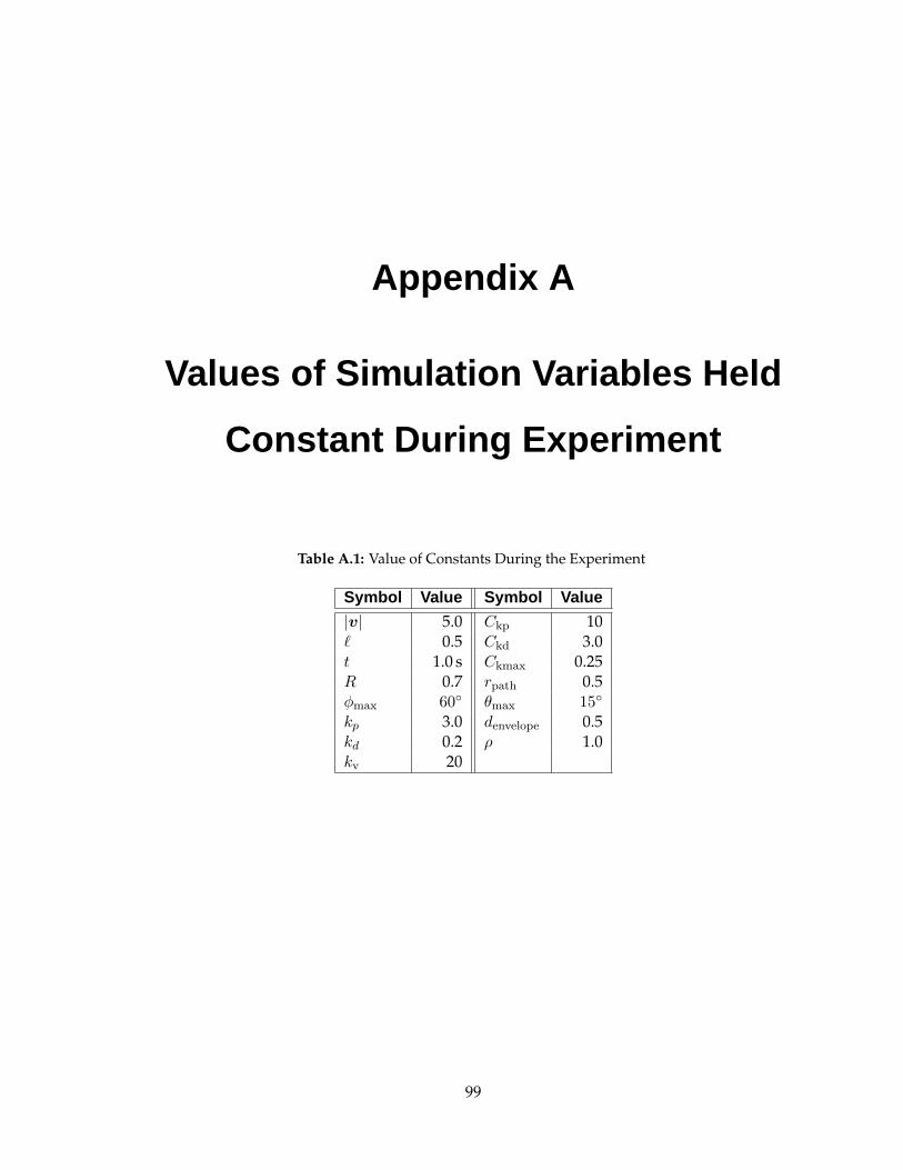
Appendix A
Values of Simulation Variables Held
Constant During Experiment
Table A.1: Value of Constants During the Experiment
Symbol Value Symbol Value
|v| 5.0 Ckp 10` 0.5 Ckd 3.0t 1.0 s Ckmax 0.25R 0.7 rpath 0.5φmax 60◦ θmax 15◦
kp 3.0 denvelope 0.5kd 0.2 ρ 1.0kv 20
99

Appendix B
Experiment Instructions
Haptic Path Guide Experiment Instructions
October 20, 2003
I am looking at how force feedback can be used to help guide a useralong a path. In this experiment you will perform a series of trialswhere you control the direction of a vehicle using a knob. Yourprimary goal is to follow the green path as closely as possible. Yoursecondary goal is to keep the center of the vehicle as close aspossible to the center of the path which is drawn as a red line.Through out the experiment you will be exposed to different forcefeedback methods, path shapes and visibility levels. You will haveapproximately 5 minutes to familiarize yourself with the pathfollowing task. After this familiarization phase the experiment willbegin when you are ready.
The experiment consists of 6 blocks of 30 trials each. Each trial willtake approximately 10 to 20 seconds. After each block of 30 trials youwill be asked to answer some questions about your experiences with thetrials in that block. At the end of the experiment I will ask you afew questions about your experiences.
Please adjust the height of your chair and the position of the knob tobe in a comfortable configuration.
If you have any questions please ask them now.
When you have finished reading this let the experimenter know and wewill start the familiarization phase.
101

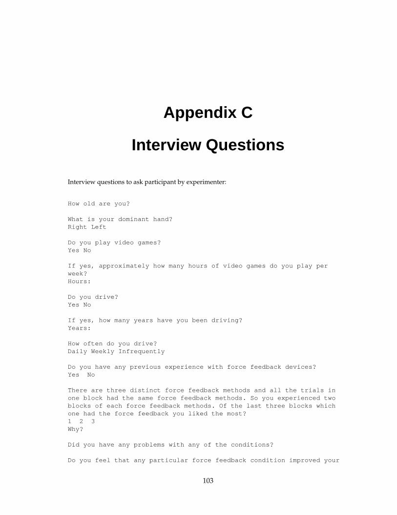
Appendix C
Interview Questions
Interview questions to ask participant by experimenter:
How old are you?
What is your dominant hand?Right Left
Do you play video games?Yes No
If yes, approximately how many hours of video games do you play perweek?Hours:
Do you drive?Yes No
If yes, how many years have you been driving?Years:
How often do you drive?Daily Weekly Infrequently
Do you have any previous experience with force feedback devices?Yes No
There are three distinct force feedback methods and all the trials inone block had the same force feedback methods. So you experienced twoblocks of each force feedback methods. Of the last three blocks whichone had the force feedback you liked the most?1 2 3Why?
Did you have any problems with any of the conditions?
Do you feel that any particular force feedback condition improved your
103

performance?
Any other questions/comments?
104
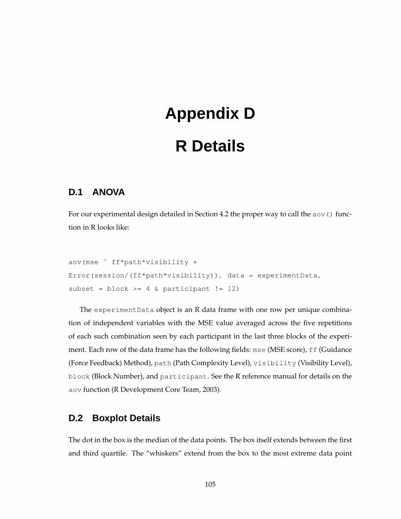
Appendix D
R Details
D.1 ANOVA
For our experimental design detailed in Section 4.2 the proper way to call the aov() func-
tion in R looks like:
aov(mse ˜ ff*path*visibility +
Error(session/(ff*path*visibility)), data = experimentData,
subset = block >= 4 & participant != 12)
The experimentData object is an R data frame with one row per unique combina-
tion of independent variables with the MSE value averaged across the five repetitions
of each such combination seen by each participant in the last three blocks of the experi-
ment. Each row of the data frame has the following fields: mse (MSE score), ff (Guidance
(Force Feedback) Method), path (Path Complexity Level), visibility (Visibility Level),
block (Block Number), and participant . See the R reference manual for details on the
aov function (R Development Core Team, 2003).
D.2 Boxplot Details
The dot in the box is the median of the data points. The box itself extends between the first
and third quartile. The “whiskers” extend from the box to the most extreme data point
105

that is no more than one and a half times the inter-quartile range (IQR). Any values falling
outside of the whiskers (called outliers) are drawn as open circles.
106
Appendix E
Experiment Consent Forms
The following three pages are a copy of the consent forms given to each experiment par-
ticipant at the beginning of a session.
107

T H E U N I V E R S I T Y O F B R I T I S H C O L U M B I A
PARTICIPANT’S COPY CONSENT FORM
Department of Computer Science
2366 Main Mall
Vancouver, B.C. Canada V6T 1Z4
tel: (604) 822-9289
tax: (604) 822-5485
Project Title: Physical and Multimodal Perception Studies
Principal Investigator: K. MacLean, tel. 822-8169
Co-Investigator: Ben Forsyth, tel. 822-9248 MSc. Candidate, Department of Computer Science
The purpose of this study is to examine changes in human performance as well as interaction
when using different types of haptic (touch sense) displays.
The task you will perform has been programmed on a computer. You will be asked to
respond to each successive task by pressing buttons on a keyboard and interacting with a haptic
display. You may be asked to wear headphones for the delivery of auditory input. Please tell the
experimenter if you find the auditory stimulus level uncomfortable, and it will be adjusted. You
will be asked to answer questions in a questionnaire and an interview as part of the experiment.
The interview will be audio taped for later analysis.
You will receive practice with specific instructions for the task before you begin (i.e., which
buttons to press for a given response). If you are not sure about any instructions, or wish to have
more practice, do not hesitate to ask.
TIME COMMITMENT: 1 hour session
HONORARIUM: You will receive $10 for participating in this experiment.
CONFIDENTIALITY: Your identity will be confidential: you will not be identified by name in any study reports. Experimental results will be stored in a secure Computer Science account accessible only to the experimenters. The anonymous data from the experiment will be used in a Master’s thesis.
You understand that the experimenter will ANSWER ANY QUESTIONS you have about the
instructions or the procedures of this study. After participating, the experimenter will answer any
questions you have about this study.
You understand that you have the RIGHT TO REFUSE to participate or to withdraw from
the study at any time without penalty of any form.
You hereby CONSENT to participate in this study and acknowledge RECEIPT of a copy of
the consent form:
If you have any concerns regarding your treatment as a research subject you may contact the
Research Subject Information Line in the UBC Office of Research Services at 604-822-8598.
Page 1 of 1 revised 8/24/2004
108

T H E U N I V E R S I T Y O F B R I T I S H C O L U M B I A
PARTICIPANT’S COPY CONSENT FORM
Department of Computer Science
2366 Main Mall
Vancouver, B.C. Canada V6T 1Z4
tel: (604) 822-9289
tax: (604) 822-5485
Project Title: Physical and Multimodal Perception Studies
Principal Investigator: K. MacLean, tel. 822-8169
Co-Investigator: Ben Forsyth, tel. 822-9248 MSc. Candidate, Department of Computer Science
The purpose of this study is to examine changes in human performance as well as interaction
when using different types of haptic (touch sense) displays.
The task you will perform has been programmed on a computer. You will be asked to
respond to each successive task by pressing buttons on a keyboard and interacting with a haptic
display. You may be asked to wear headphones for the delivery of auditory input. Please tell the
experimenter if you find the auditory stimulus level uncomfortable, and it will be adjusted. You
will be asked to answer questions in a questionnaire and an interview as part of the experiment.
The interview will be audio taped for later analysis.
You will receive practice with specific instructions for the task before you begin (i.e., which
buttons to press for a given response). If you are not sure about any instructions, or wish to have
more practice, do not hesitate to ask.
TIME COMMITMENT: 1 hour session
HONORARIUM: You will receive $10 for participating in this experiment.
CONFIDENTIALITY: Your identity will be confidential: you will not be identified by name in any study reports. Experimental results will be stored in a secure Computer Science account accessible only to the experimenters. The anonymous data from the experiment will be used in a Master’s thesis.
You understand that the experimenter will ANSWER ANY QUESTIONS you have about the
instructions or the procedures of this study. After participating, the experimenter will answer any
questions you have about this study.
You understand that you have the RIGHT TO REFUSE to participate or to withdraw from
the study at any time without penalty of any form.
You hereby CONSENT to participate in this study and acknowledge RECEIPT of a copy of
the consent form:
If you have any concerns regarding your treatment as a research subject you may contact the
Research Subject Information Line in the UBC Office of Research Services at 604-822-8598.
Page 1 of 1 revised 8/24/2004
109

T H E U N I V E R S I T Y O F B R I T I S H C O L U M B I A
RESEARCHER’S COPY CONSENT FORM
Department of Computer Science
2366 Main Mall
Vancouver, B.C. Canada V6T 1Z4
tel: (604) 822-9289
tax: (604) 822-5485
Project Title: Physical and Multimodal Perception Studies
Principal Investigator: K. MacLean, tel. 822-8169
Co-Investigator: Ben Forsyth, tel. 822-9248 MSc. Candidate, Department of Computer Science
The purpose of this study is to examine changes in human performance as well as interaction
when using different types of haptic (touch sense) displays.
The task you will perform has been programmed on a computer. You will be asked to
respond to each successive task by pressing buttons on a keyboard and interacting with a haptic
display. You may be asked to wear headphones for the delivery of auditory input. Please tell the
experimenter if you find the auditory stimulus level uncomfortable, and it will be adjusted. You
will be asked to answer questions in a questionnaire and an interview as part of the experiment.
The interview will be audio taped for later analysis.
You will receive practice with specific instructions for the task before you begin (i.e., which
buttons to press for a given response). If you are not sure about any instructions, or wish to have
more practice, do not hesitate to ask.
TIME COMMITMENT: 1 hour session
HONORARIUM: You will receive $10 for participating in this experiment.
CONFIDENTIALITY: Your identity will be confidential: you will not be identified by name in any study reports. Experimental results will be stored in a secure Computer Science account accessible only to the experimenters. The anonymous data from the experiment will be used in a Master’s thesis.
You understand that the experimenter will ANSWER ANY QUESTIONS you have about the
instructions or the procedures of this study. After participating, the experimenter will answer any
questions you have about this study.
You understand that you have the RIGHT TO REFUSE to participate or to withdraw from
the study at any time without penalty of any form.
Page 1 of 2 revised 8/24/2004
110

T H E U N I V E R S I T Y O F B R I T I S H C O L U M B I A
You hereby CONSENT to participate in this study and acknowledge RECEIPT of a copy of
the consent form:
NAME
(please print)
SIGNATURE DATE
If you have any concerns regarding your treatment as a research subject you may contact the
Research Subject Information Line in the UBC Office of Research Services at 604-822-8598.
Page 2 of 2 revised 8/24/2004
111

Appendix F
Raw Data
The following pages are the path trajectories for every participant over the last three blocks.
There are three pages per participant, one for each of the guidance methods. The trials on
a given page were thus executed during the same block (30 trials). Trials on each page are
organized by path type (zigzag, bump, and curve). The plots contain trials with both vis-
ibility levels to conserve space. Thus there are ten trials per path type, evenly distributed
(on average) between the reflections of each path type.
Participant 13 was the discarded outlier. Of the 17 participants used in the analysis
participant 1 has the worst performance and participant 6 has the best.
113
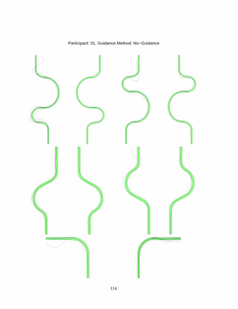
Participant: 01, Guidance Method: No−Guidance
114
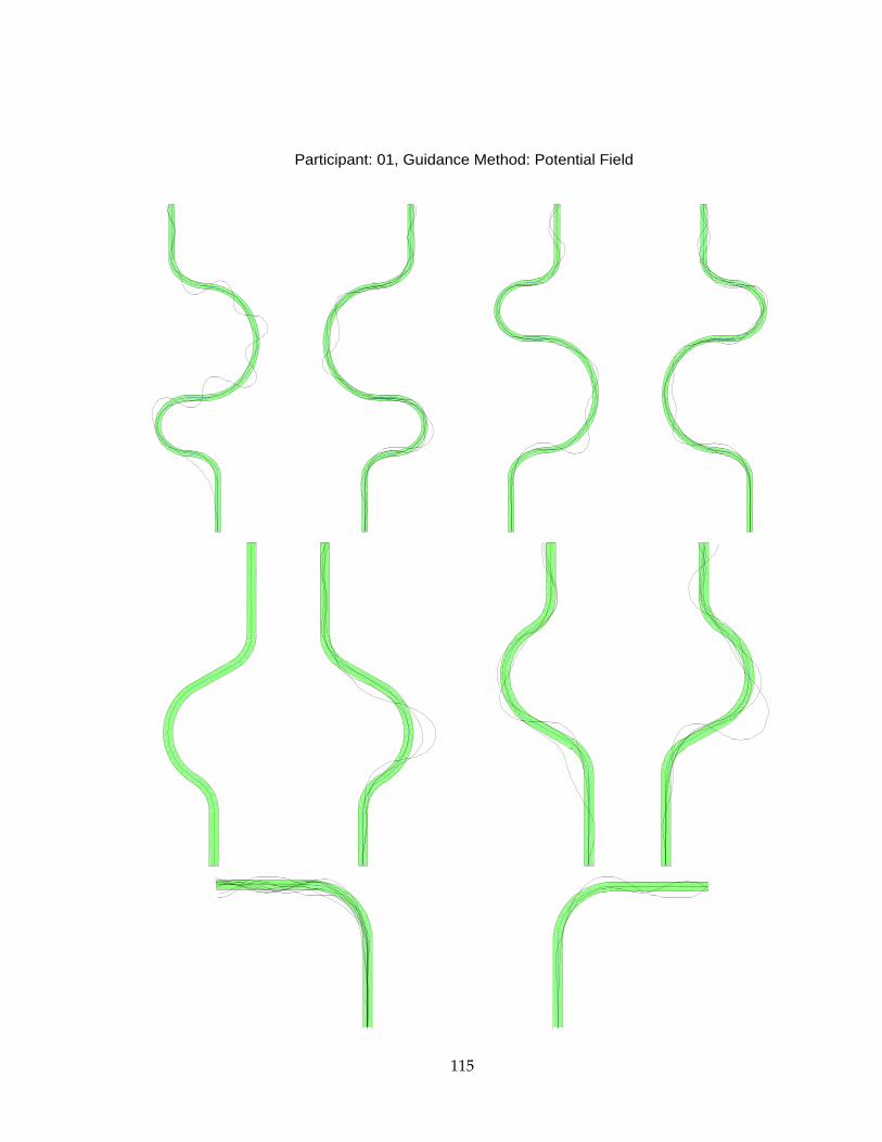
Participant: 01, Guidance Method: Potential Field
115
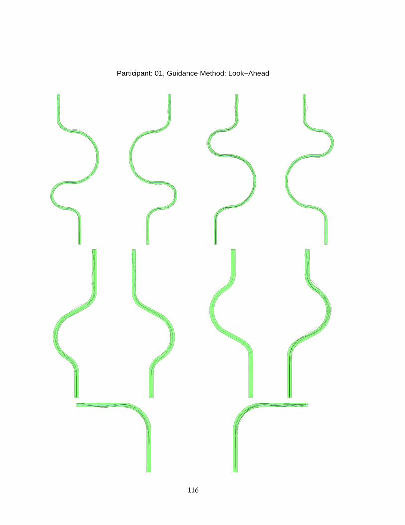
Participant: 01, Guidance Method: Look−Ahead
116
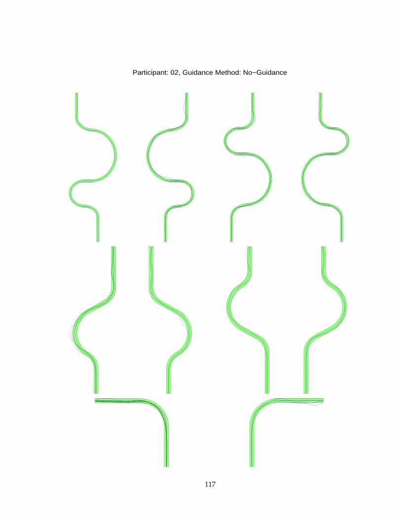
Participant: 02, Guidance Method: No−Guidance
117
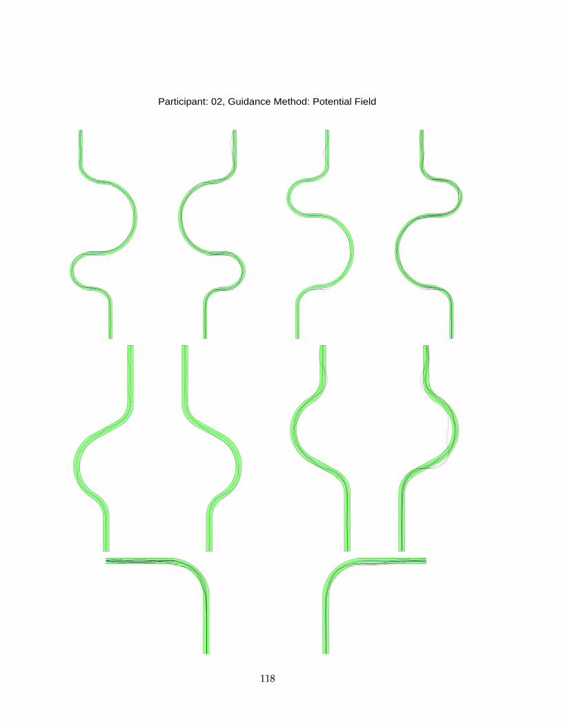
Participant: 02, Guidance Method: Potential Field
118
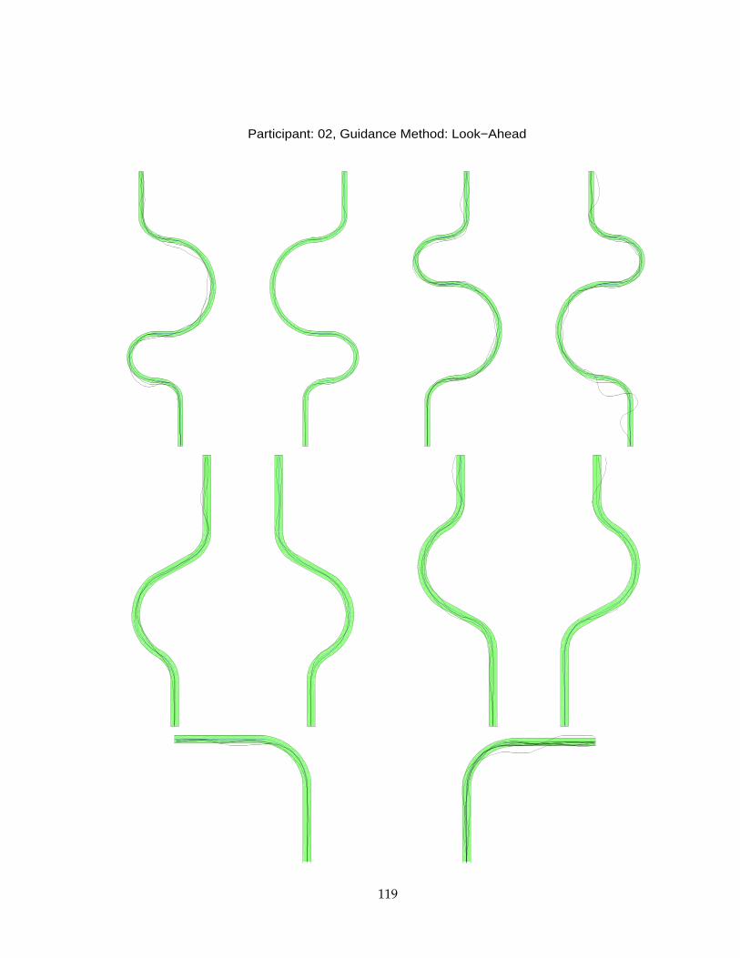
Participant: 02, Guidance Method: Look−Ahead
119
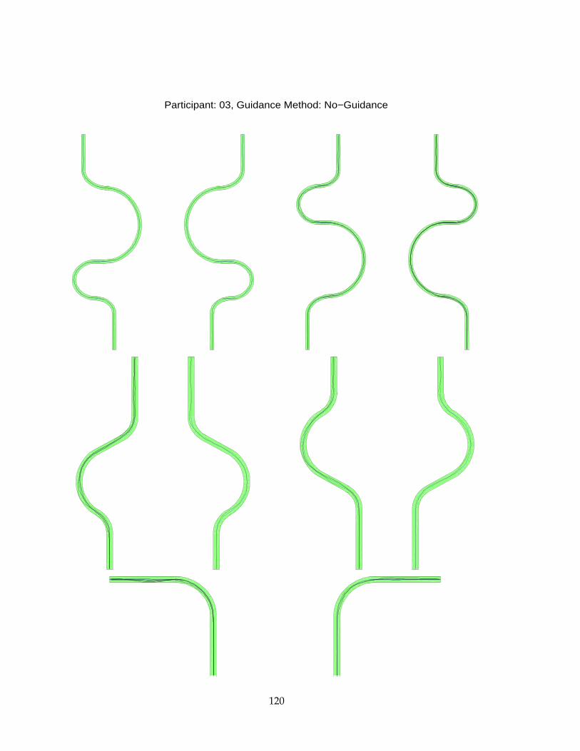
Participant: 03, Guidance Method: No−Guidance
120
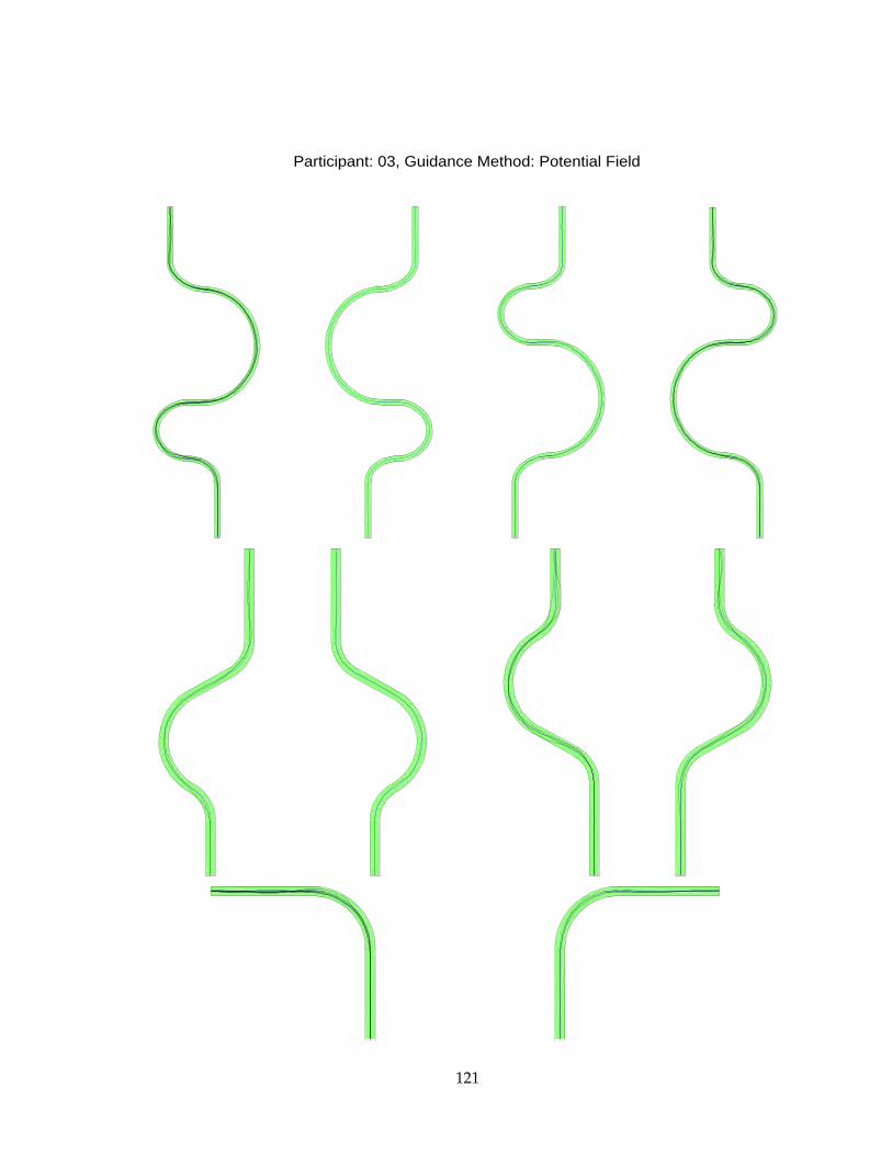
Participant: 03, Guidance Method: Potential Field
121
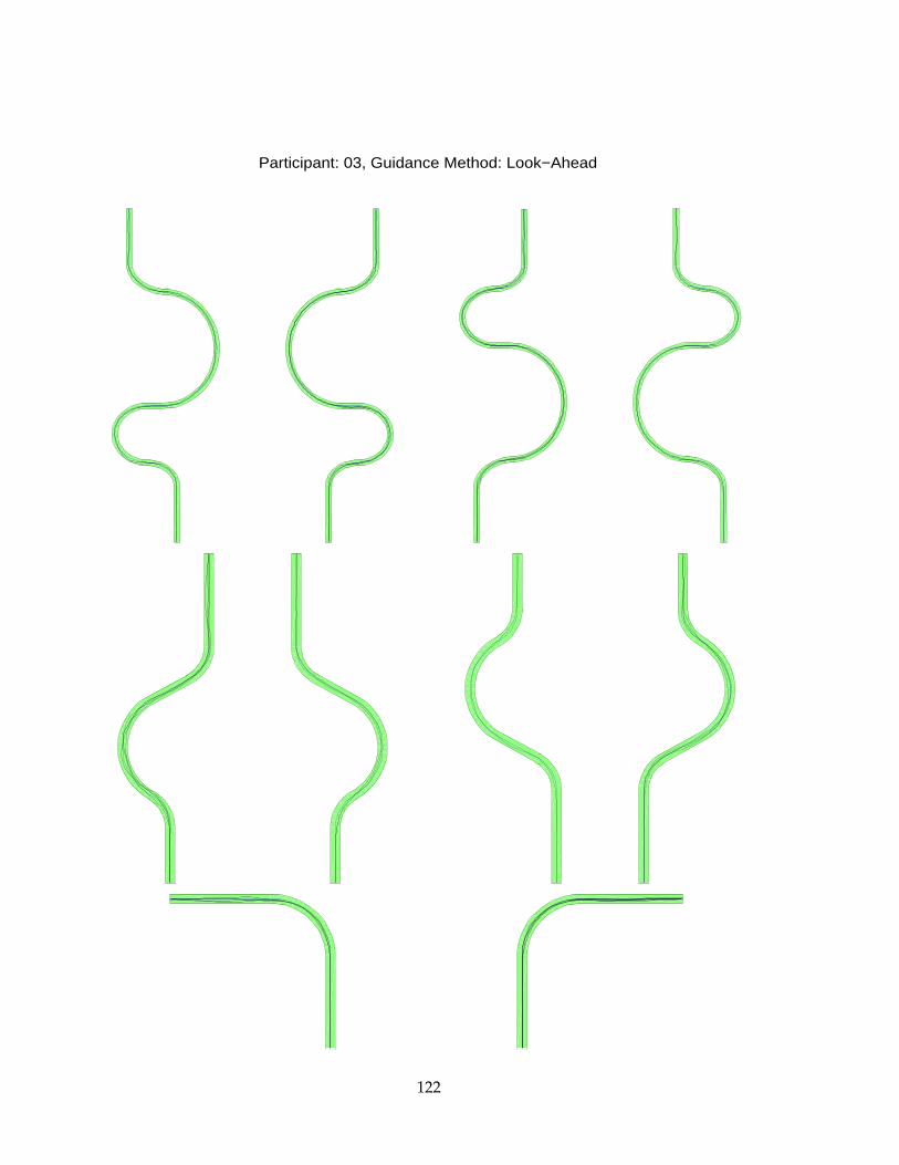
Participant: 03, Guidance Method: Look−Ahead
122
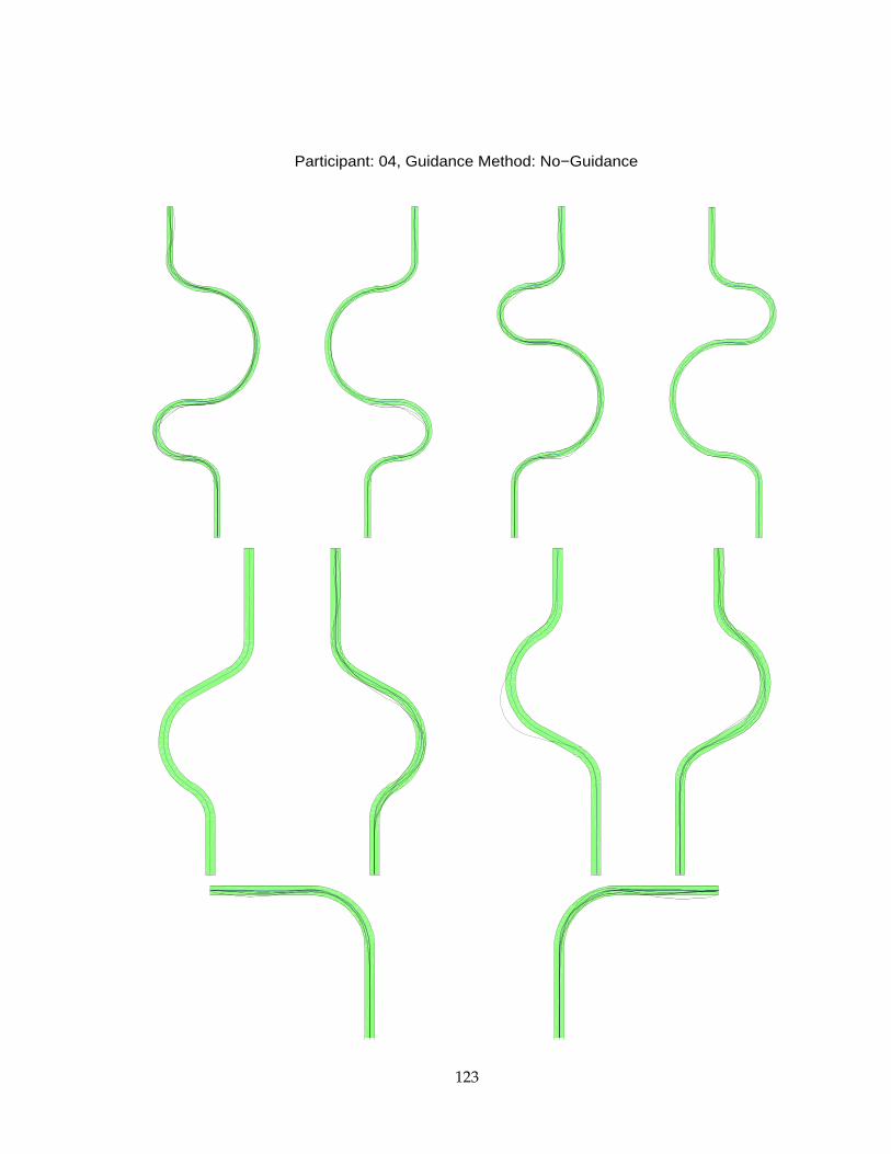
Participant: 04, Guidance Method: No−Guidance
123
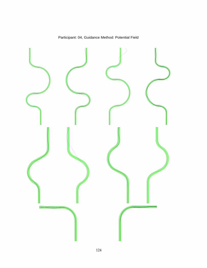
Participant: 04, Guidance Method: Potential Field
124
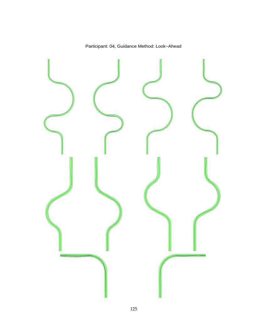
Participant: 04, Guidance Method: Look−Ahead
125
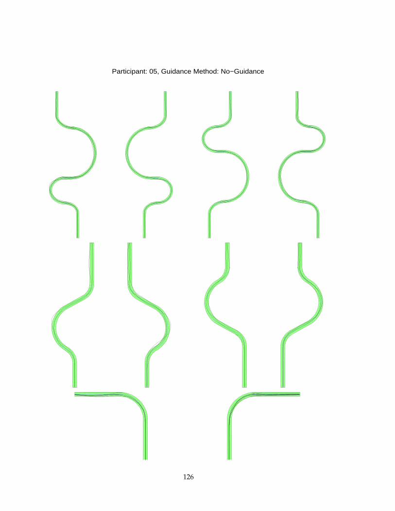
Participant: 05, Guidance Method: No−Guidance
126
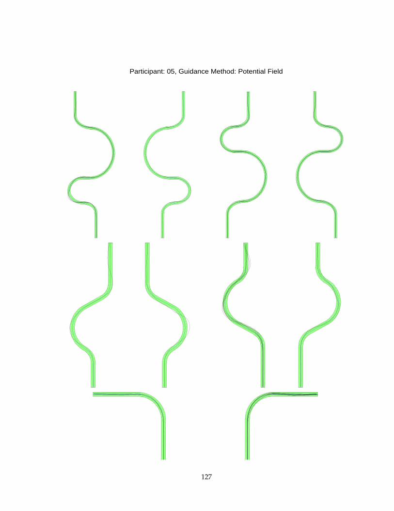
Participant: 05, Guidance Method: Potential Field
127
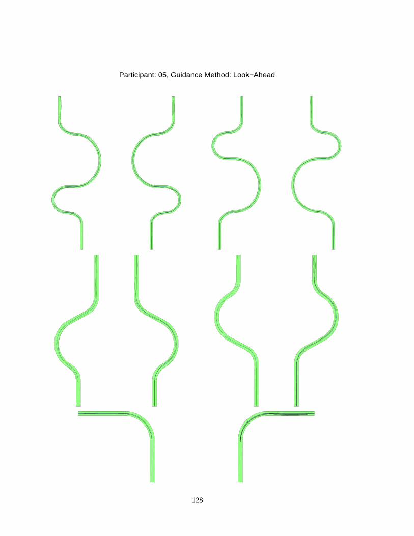
Participant: 05, Guidance Method: Look−Ahead
128
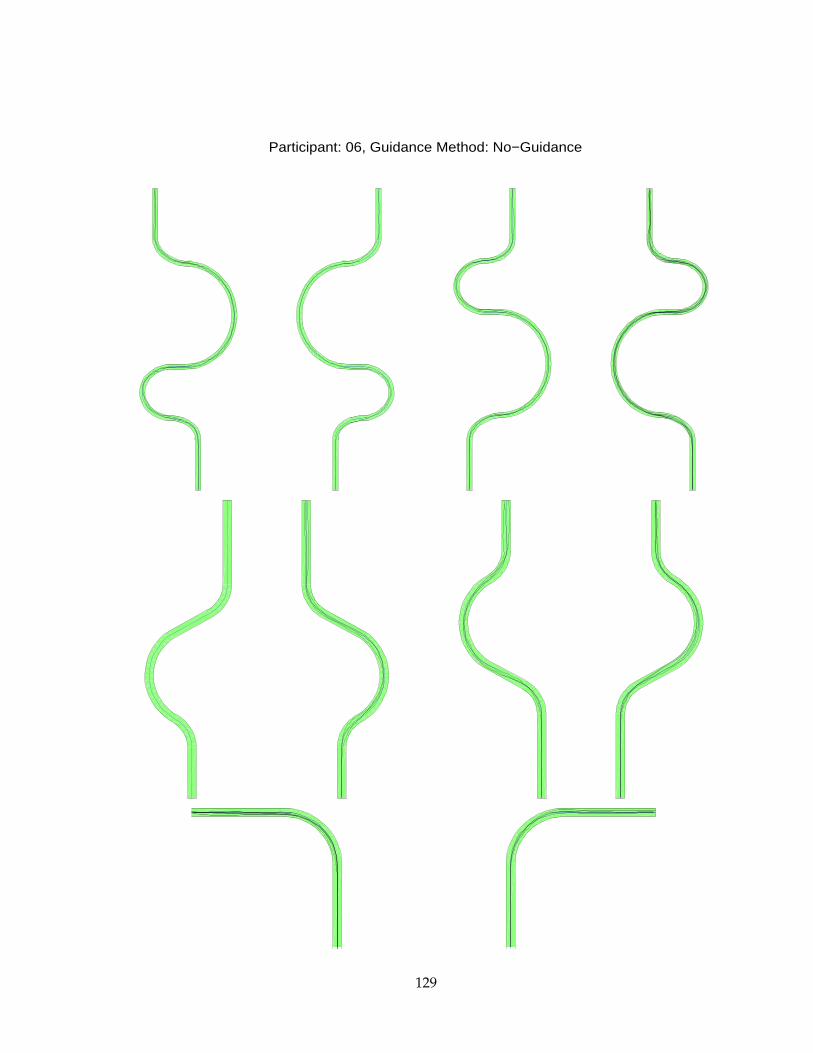
Participant: 06, Guidance Method: No−Guidance
129
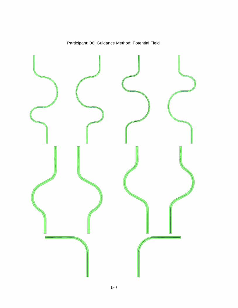
Participant: 06, Guidance Method: Potential Field
130

Participant: 06, Guidance Method: Look−Ahead
131
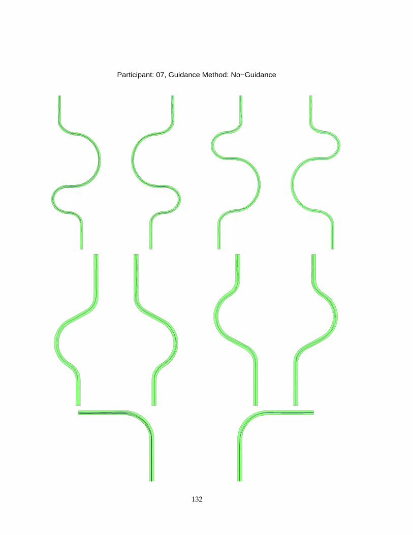
Participant: 07, Guidance Method: No−Guidance
132
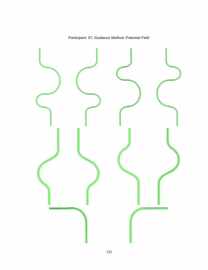
Participant: 07, Guidance Method: Potential Field
133
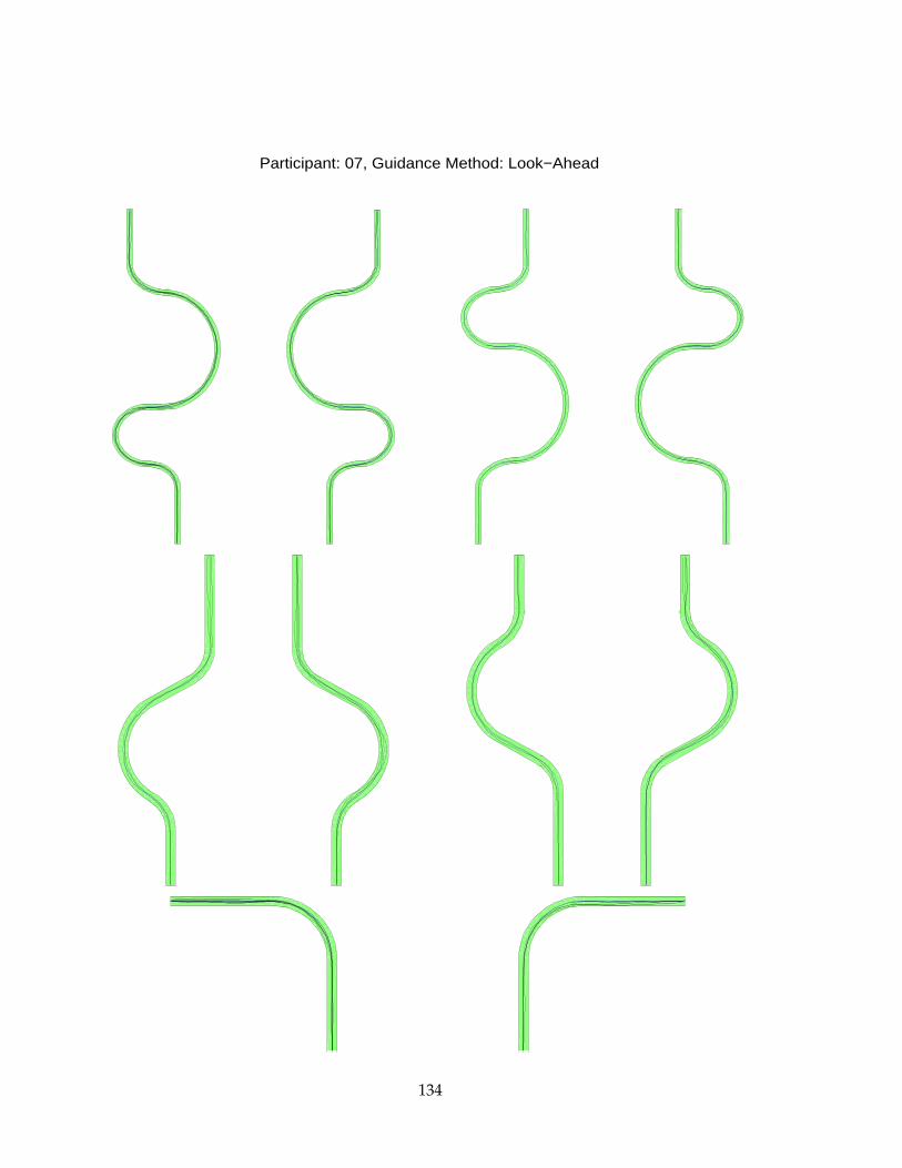
Participant: 07, Guidance Method: Look−Ahead
134
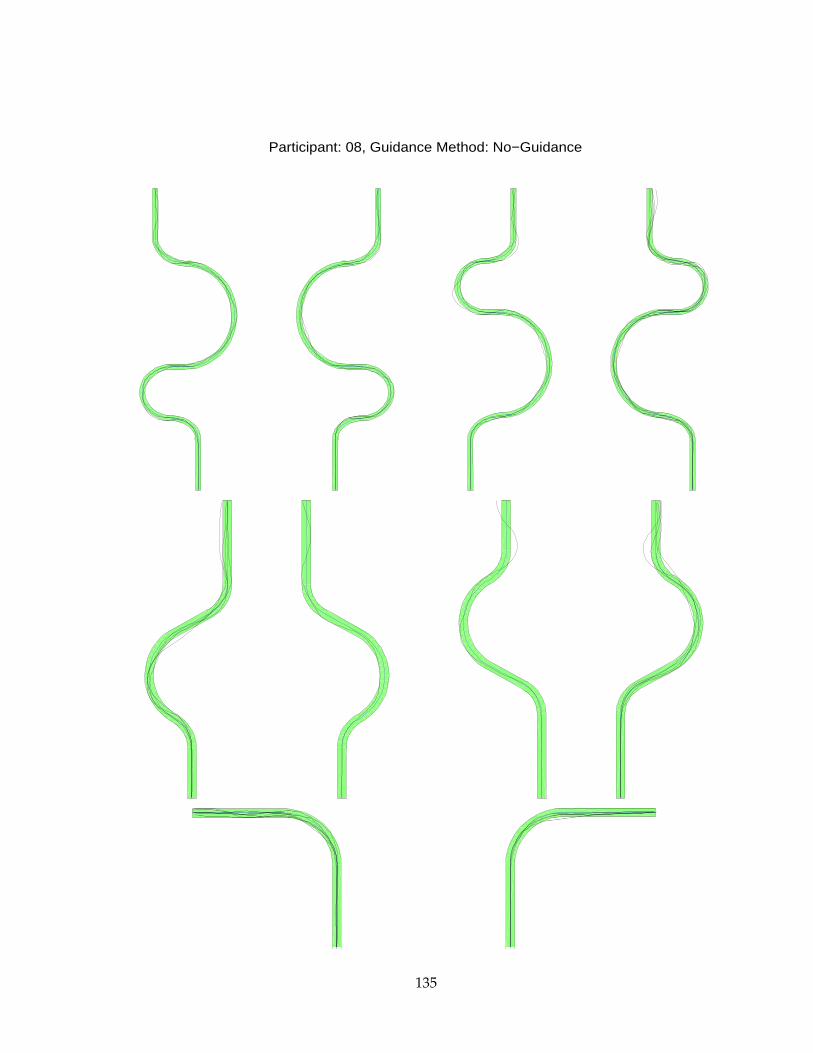
Participant: 08, Guidance Method: No−Guidance
135
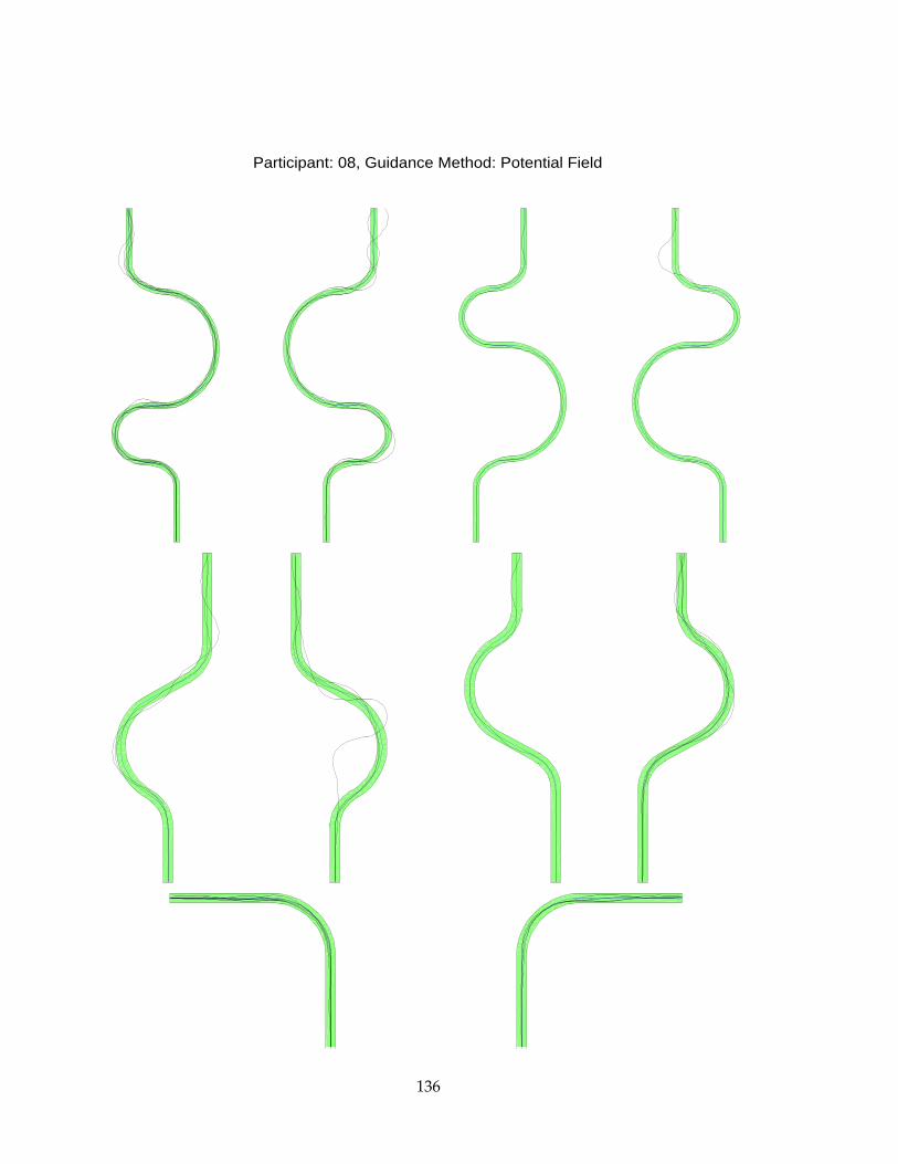
Participant: 08, Guidance Method: Potential Field
136
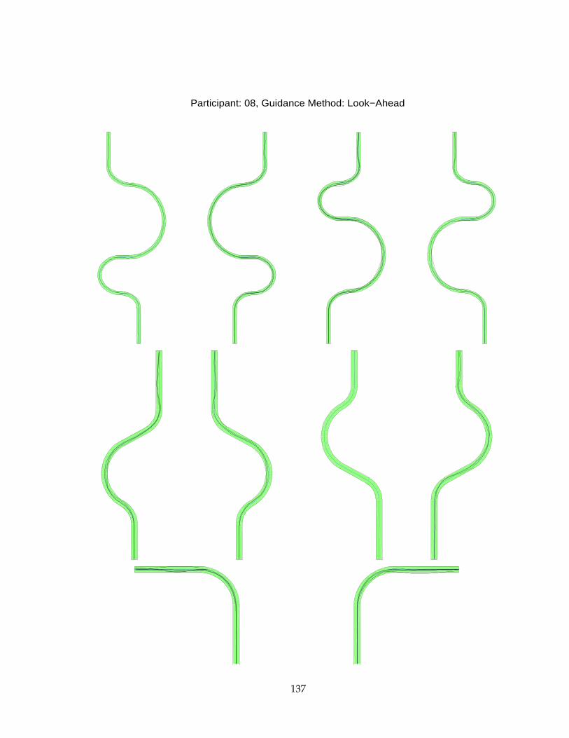
Participant: 08, Guidance Method: Look−Ahead
137
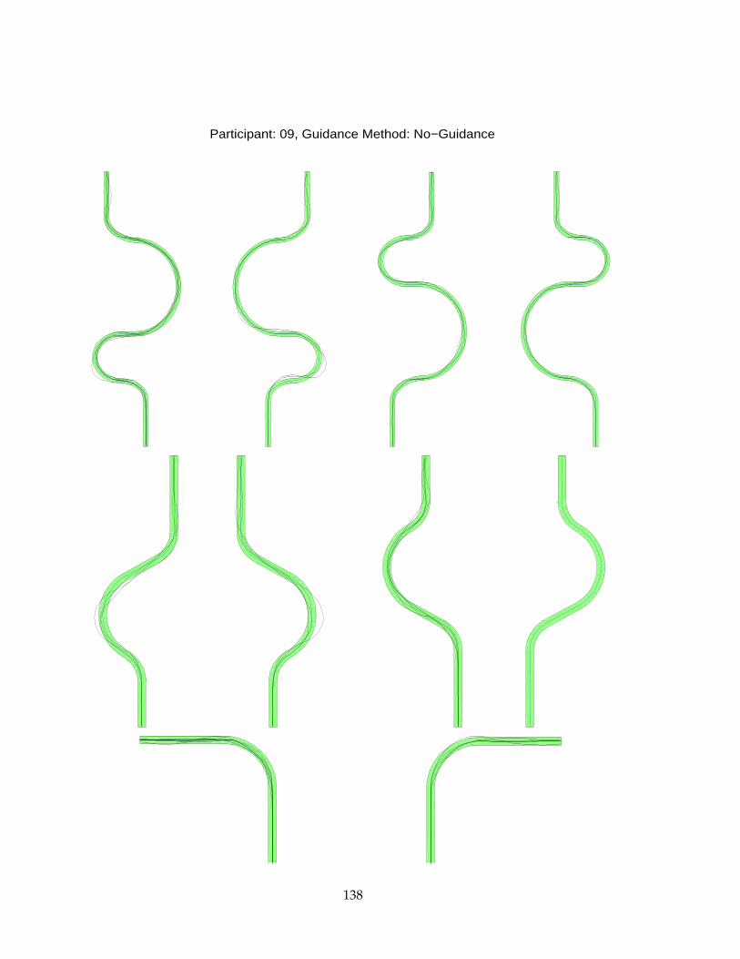
Participant: 09, Guidance Method: No−Guidance
138

Participant: 09, Guidance Method: Potential Field
139
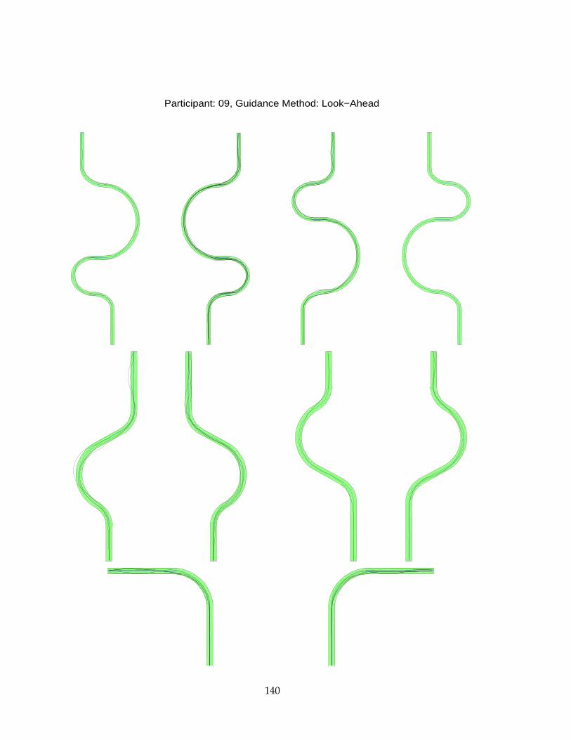
Participant: 09, Guidance Method: Look−Ahead
140

Participant: 10, Guidance Method: No−Guidance
141
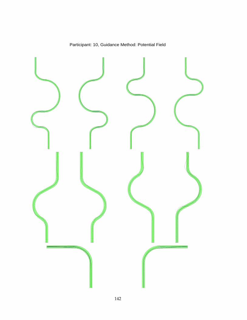
Participant: 10, Guidance Method: Potential Field
142
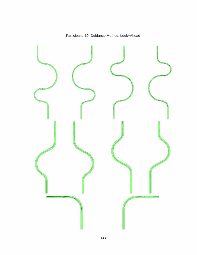
Participant: 10, Guidance Method: Look−Ahead
143

Participant: 11, Guidance Method: No−Guidance
144
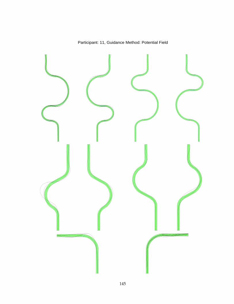
Participant: 11, Guidance Method: Potential Field
145
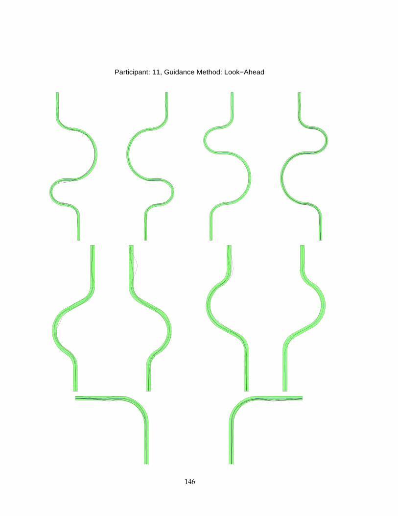
Participant: 11, Guidance Method: Look−Ahead
146
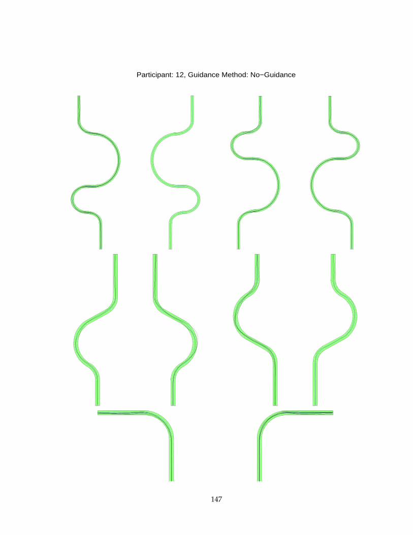
Participant: 12, Guidance Method: No−Guidance
147
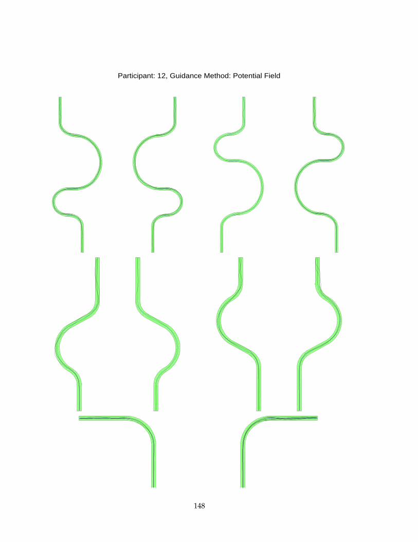
Participant: 12, Guidance Method: Potential Field
148
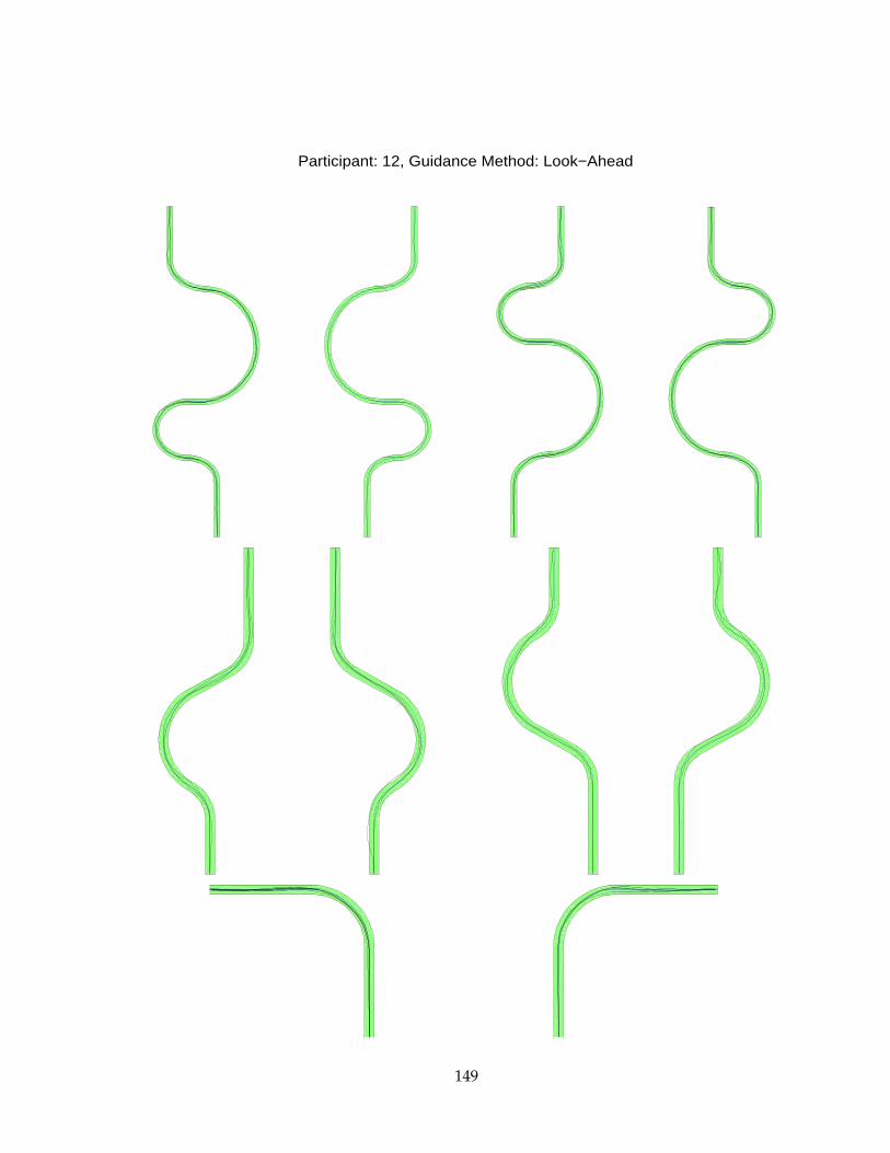
Participant: 12, Guidance Method: Look−Ahead
149
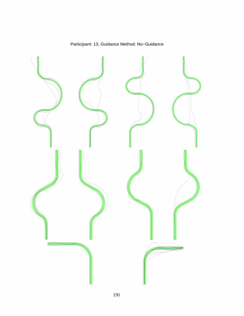
Participant: 13, Guidance Method: No−Guidance
150
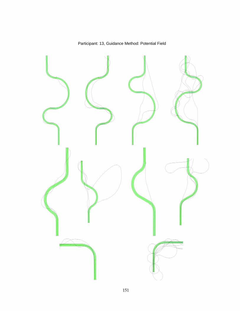
Participant: 13, Guidance Method: Potential Field
151
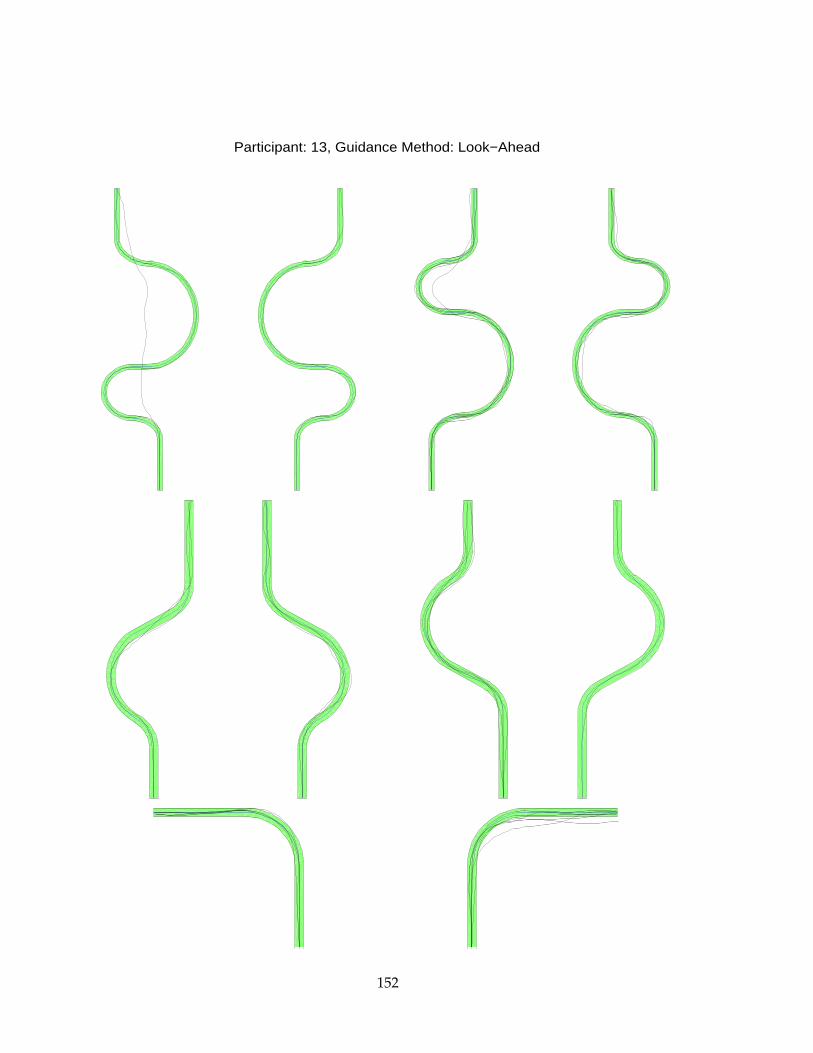
Participant: 13, Guidance Method: Look−Ahead
152
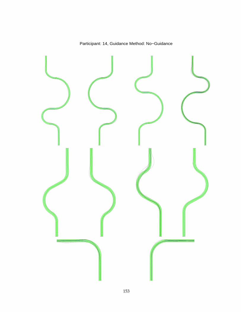
Participant: 14, Guidance Method: No−Guidance
153
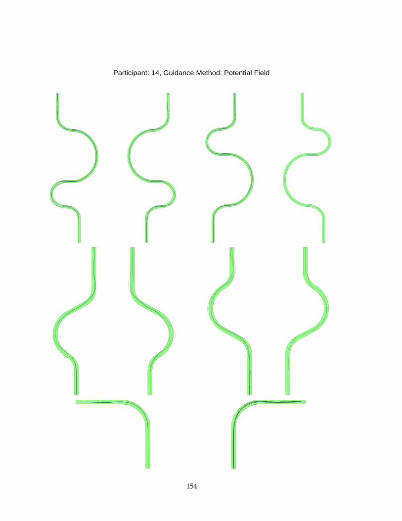
Participant: 14, Guidance Method: Potential Field
154
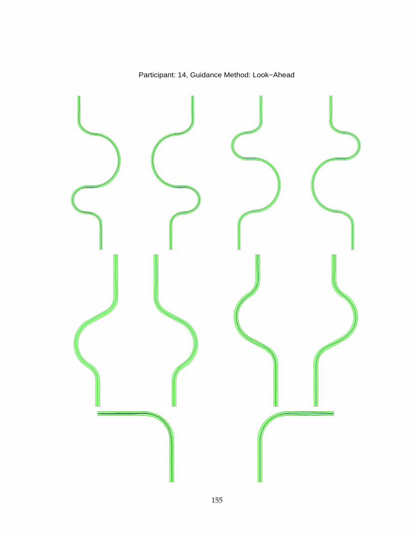
Participant: 14, Guidance Method: Look−Ahead
155
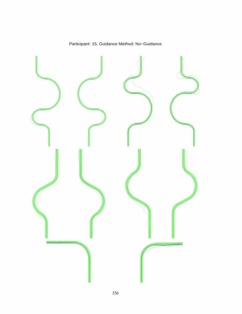
Participant: 15, Guidance Method: No−Guidance
156
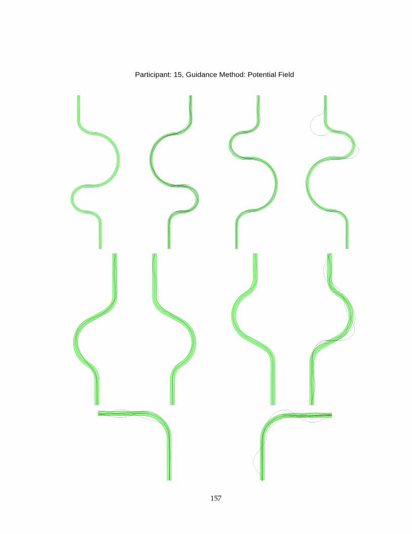
Participant: 15, Guidance Method: Potential Field
157
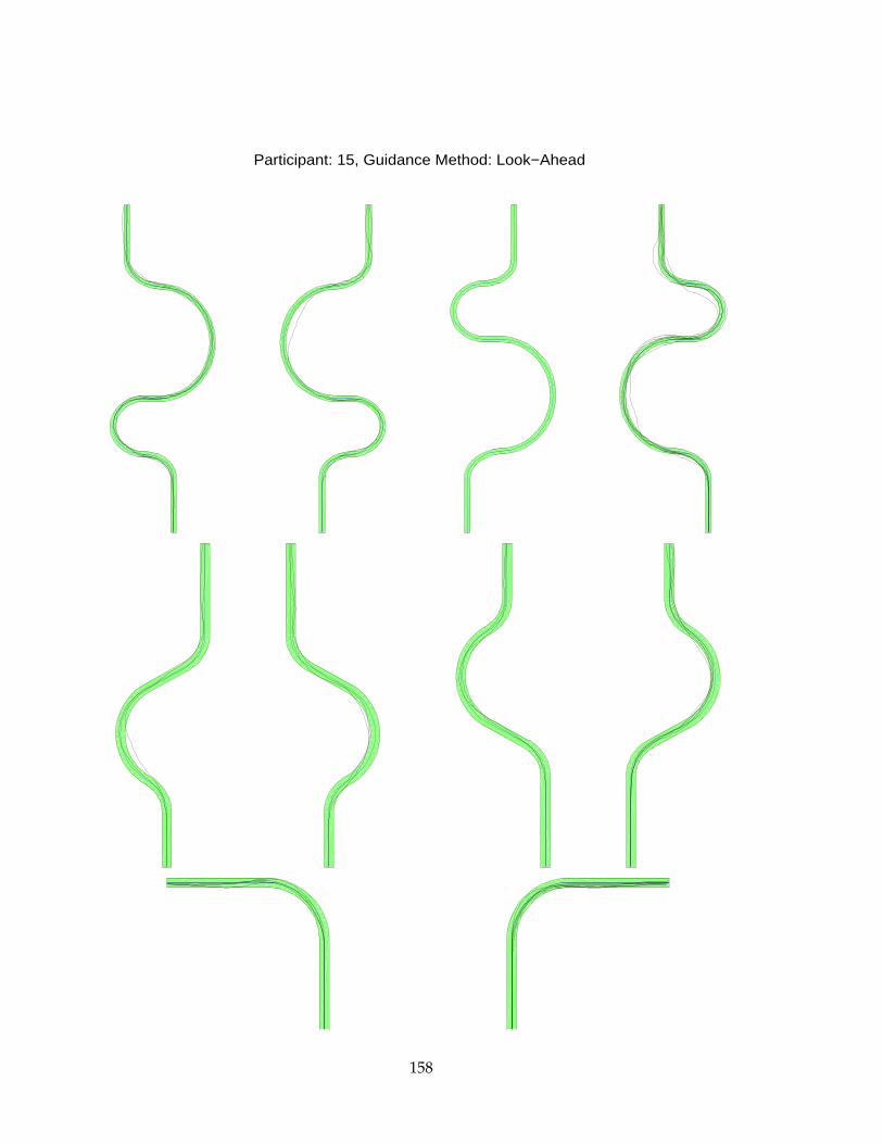
Participant: 15, Guidance Method: Look−Ahead
158
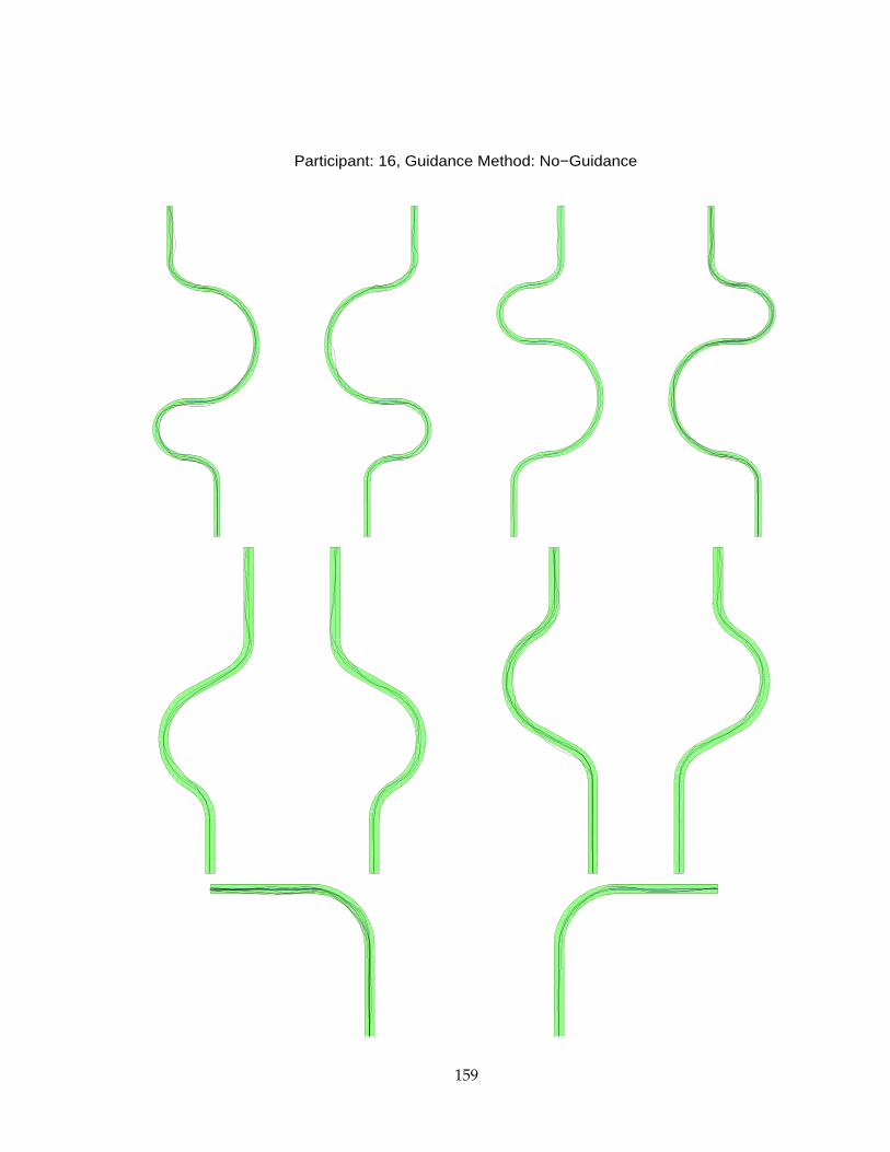
Participant: 16, Guidance Method: No−Guidance
159
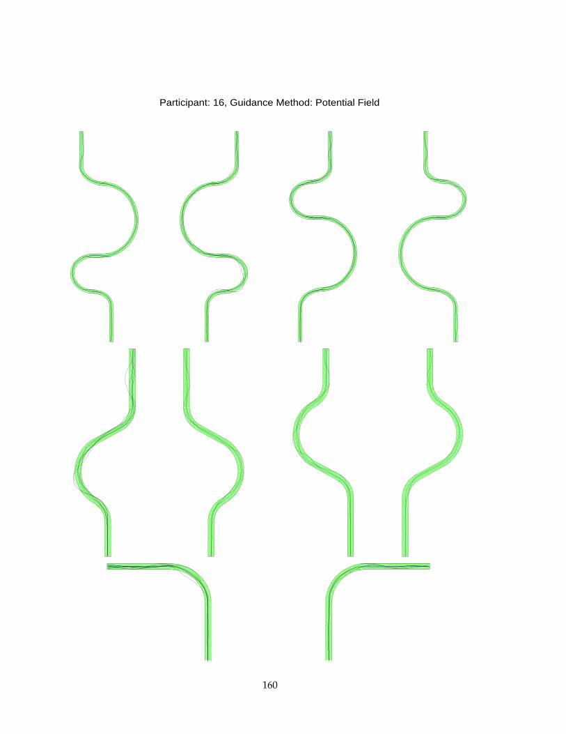
Participant: 16, Guidance Method: Potential Field
160
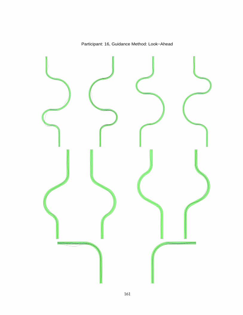
Participant: 16, Guidance Method: Look−Ahead
161
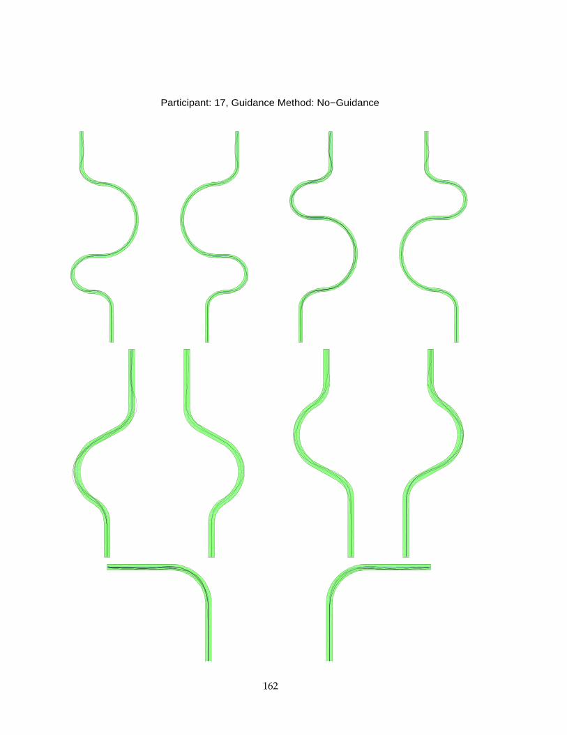
Participant: 17, Guidance Method: No−Guidance
162
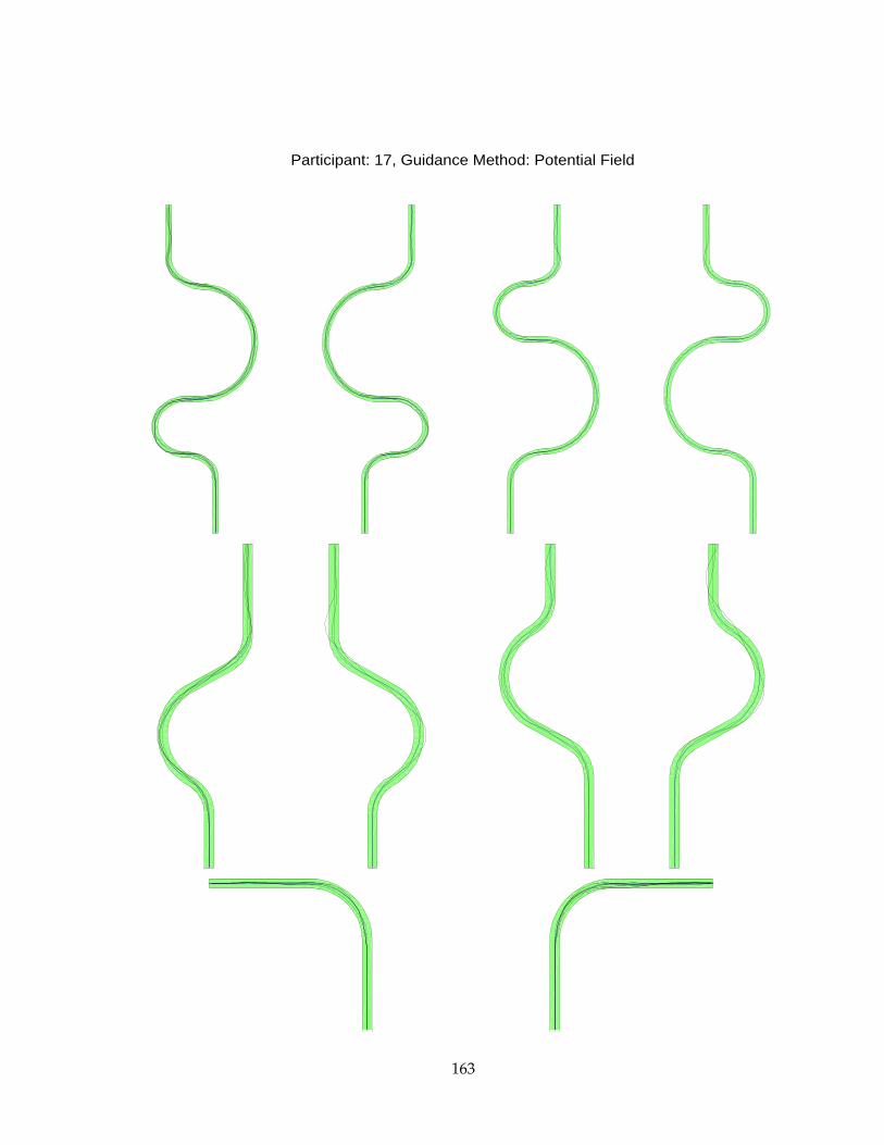
Participant: 17, Guidance Method: Potential Field
163
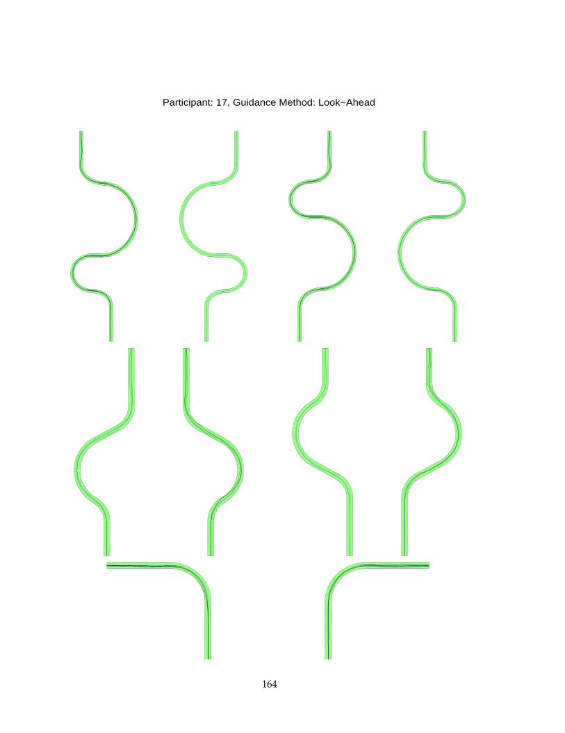
Participant: 17, Guidance Method: Look−Ahead
164
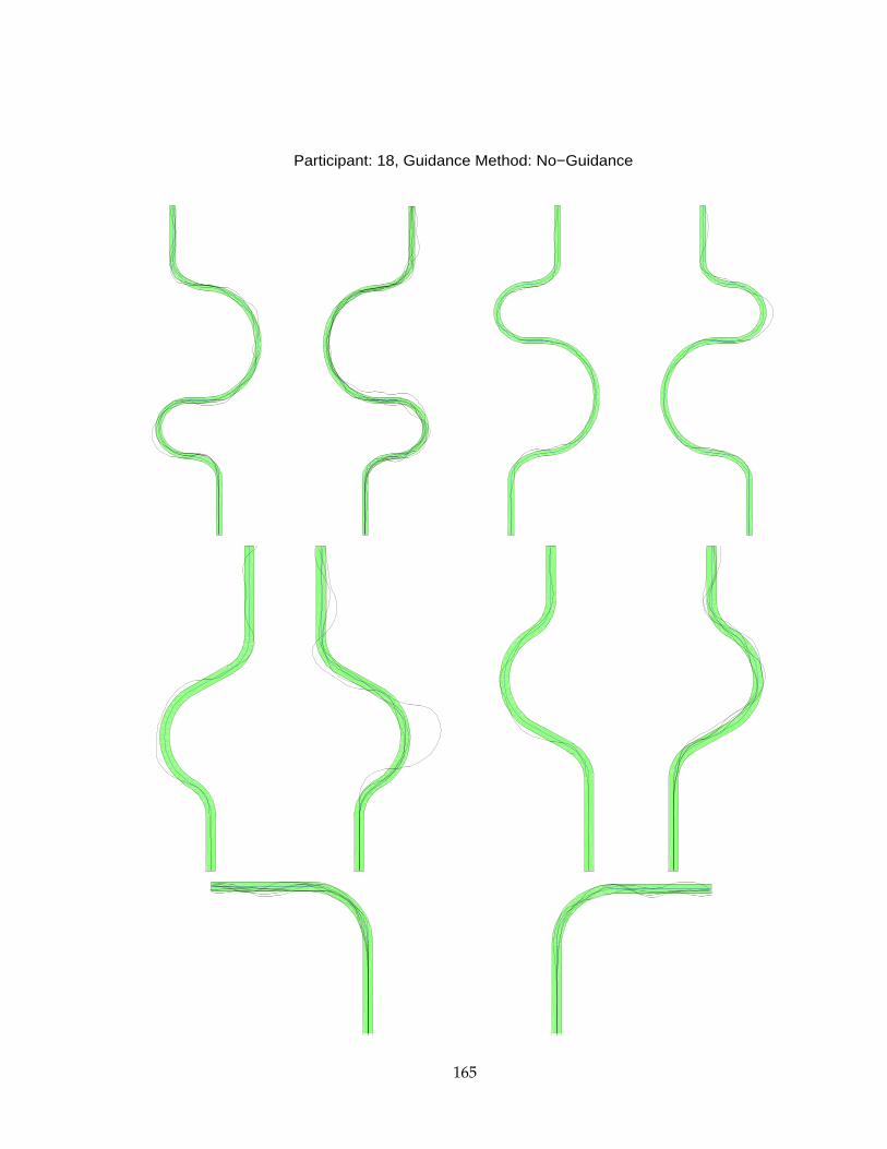
Participant: 18, Guidance Method: No−Guidance
165
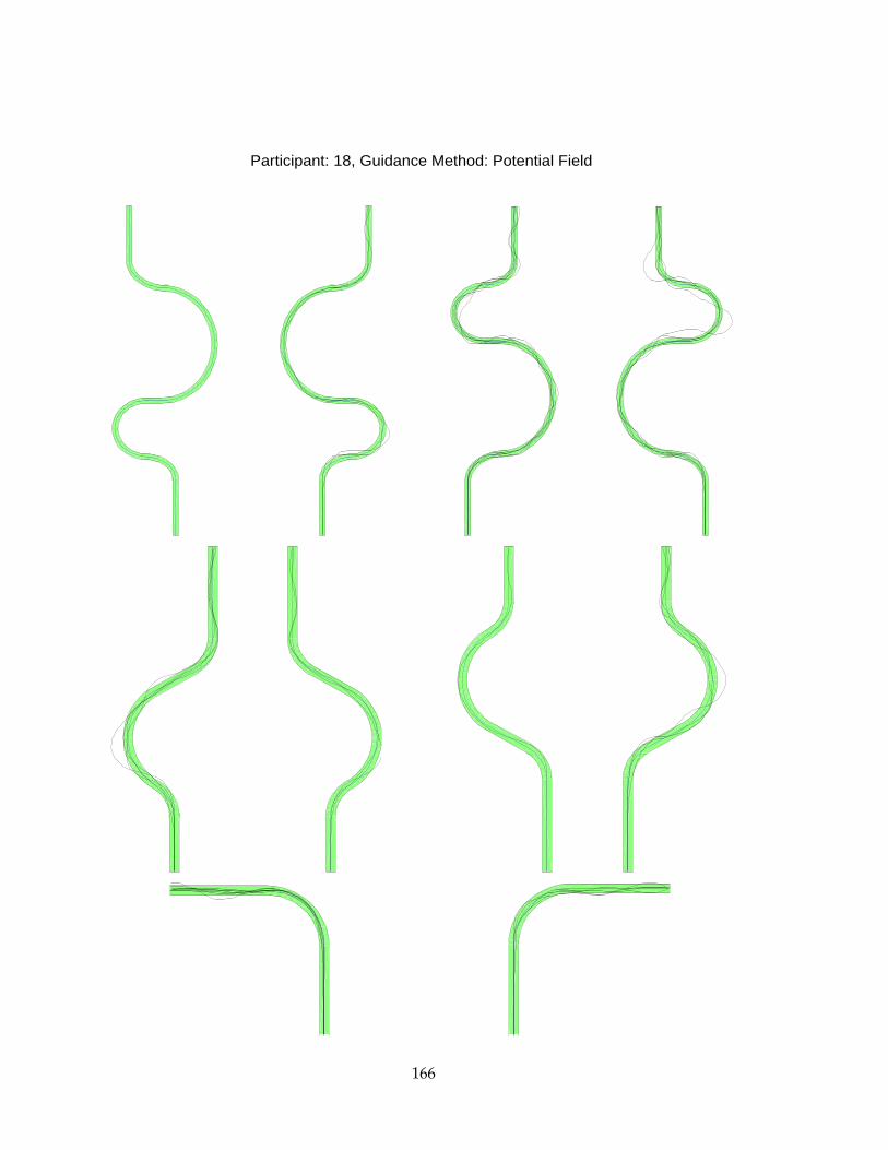
Participant: 18, Guidance Method: Potential Field
166
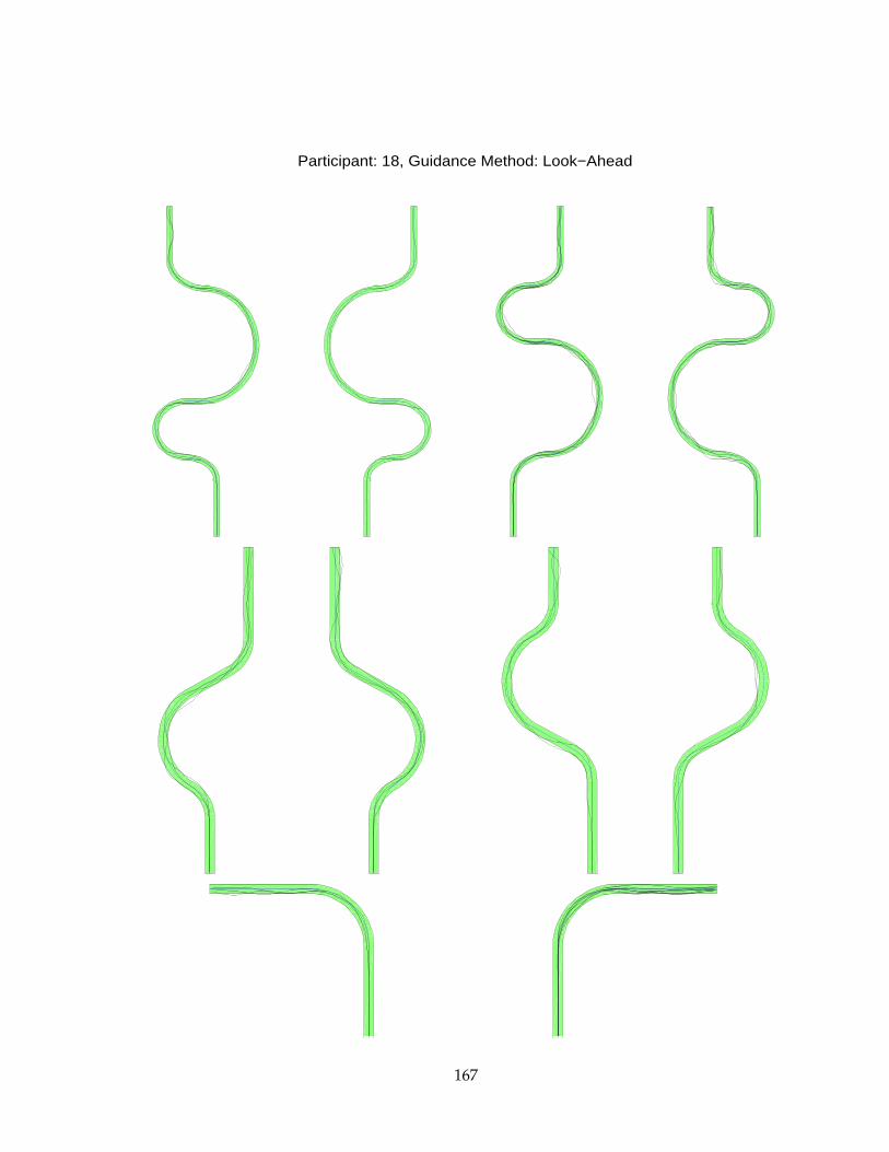
Participant: 18, Guidance Method: Look−Ahead
167