1

Intelligent Transportation Network System

ITNS

Control J. E. Anderson

September 2018

2

Contents Page

1 Introduction 3

2 Asynchronous Point-Follower Control 17

3 Controlling Many vehicles 38

5 Maneuvers 114

6 Potential Headway Violation upon Decelerating into a Station 159

7 Headway needed to delay Speed Reduction 168

8 On-Line Deceleration 170

9 Encoder Calibration 180

10 Simulation Summary 203

11 Simulate ITNS 206

12 Requirements for ITNS Control 228

13 Distance to Slip 230

15 Potential Headway Violation upon Decelerating into a Station 239

16 Some History of PRT Simulation Programs 248

End 261

3

Control of Personal Rapid Transit Systems

J. Edward Anderson

Abstract

The problem of precise longitudinal control of vehicles to follow predetermined time-varying speeds and positions has been solved. To control vehicles to the required close headway of at least 0.5 sec, the control philosophy is different from but no less rigorous than that of railroad practice. A PRT system can be designed with as good a safety record as any existing transit system and, because of the ease of adequate passenger protection, quite likely much better. The basis for the control of a fleet of PRT vehicles of arbitrary size is a complete set of maneuver equations. The author's conclusion is that the preferred control strategy is one that could be called an "asynchronous point follower." Such a strategy requires no clock synchronization, is flexible in the face of all unusual conditions, permits the maximum possible throughput, requires a minimum of maneuvering and uses a minimum of software. Since each vehicle is controlled independently, there is no string instability. Since the wayside zone controllers have in their memory the same maneuver equations as the on-board computers, accurate safety monitoring is practical. To obtain sufficiently high reliability, careful failure modes and effects analysis must be a key part of the design process, and the control computers must be checked redundant.

Introduction

The problem of closed-loop automatic longitudinal control of a single vehicle constrained to follow a guideway at a specified time-varying speed and position within adequate accuracy has been solved by several investigators [1, 2], and analytical equations for the required speed and position gains have been derived. The architecture of checked redundant microprocessor control for automated transit vehicles has been developed and has been shown to be able to achieve a safety record as good or better than a modern rapid rail system [3]. The major challenge in PRT control has been to control a large fleet of vehicles operating at fractional-second headway and merging and diverging in and out of stations and between separate branches in a network of guideways with an acceptable level of safety, comfort, and dependability, while meeting other essential criteria. A great deal of work has been done on this problem over the past few decades. Much of the published work can be found in conference proceedings [4, 5, 6], in papers referenced in those proceedings, and in results of the Urban Mass Transportation Administration's Advanced Group Rapid Transit Program [7, 8]. While the AGRT system was designed for 3-sec headway, much of the work is directly applicable to PRT. Together with the work of The Aerospace Corporation PRT Program [9] and the DEMAG+MBB Cabintaxi PRT Program [10], one can obtain an excellent perspective on the field.

In a short paper, it is not possible to describe any appreciable portion of this work, but it is more useful to give a synthesis of conclusions reached concerning the means of controlling a PRT system, which have been built on the shoulders of prior investigators. I first discuss the criteria any PRT control system must meet. Then, it is necessary to discuss the problem of safe achievement of adequately low time headway between vehicles and how the safety philosophy

4

must differ from standard railroad practice. Next is a discussion of strategies of control of many vehicles in a network. With this background, the next topics are the information that must be available on board the vehicles and at various wayside points, the sensing and communication requirements, and the mathematics involved. I do not discuss lateral control because, in most PRT systems, wheels running against lateral surfaces achieve it passively.

Control Criteria

Line and Station Throughput

Analysis of PRT networks in many applications has shown that fractional-second headways are both needed and attainable. The 1974 UMTA Administrator Frank Herringer, in testimony before a committee of the Congress of the United States, said: "A DOT program leading to the development of a short, one-half to one-second headway, high-capacity PRT system will be initiated in fiscal year 1974 [11]." This statement was a result of consensus among workers in the PRT field in consultation with the Research and Development staff of UMTA on the need and practicality of headways as low as 0.5 sec. Off-line stations must be designed to meet expected input and output flows, and the system must be designed to prevent excessive congestion at merge points and destination stations.

Safety

A PRT system must provide a level of safety in terms of injuries per 100 million miles at least as good as a modern rapid rail system [3], and preferably better because the improvements provided by PRT in all areas must be good enough to justify the development cost. To achieve this level of safety, the on-board and wayside computers must be checked redundant.

Dependability

The term "dependability" is less often used than "availability," which is measurable in conventional transit systems as the percentage of trains that arrive at stations when expected. The quantity dependability, which is the ratio of person-hours not delayed to the number of person-hours of operation, is a more meaningful criteria and, in PRT, can be easily measured and updated trip by trip by a central computer [12]. In a recent PRT program, it was specified that the undependability (1 - dependability) should be no more than 3 person-hours of delay per 1000 person-hours of operation. From our analysis, if the safety criterion is met, the undependability will be at least an order of magnitude less.

Ride Comfort

Longitudinal maneuvers must be performed in such a way that International Standards Organization ride comfort standards on acceleration as a function of frequency are met. As to maneuvers, the National Maglev Initiative Office set the most recent federal standards on ride comfort that would be applicable to vehicles in which all passengers are seated. They restrict acceleration to 0.2 g and jerk to 0.25 g/s in normal operation. The maximum emergency-braking

5

deceleration depends on whether passenger constraints are provided. If not, the criterion must be that the passenger does not slide off the seat in an emergency stop.

Changing Conditions

The control system must be able to reduce cruising speed in high winds and must be able to cope with any unusual situation, such as a stopped vehicle, that would require vehicles to slow down or stop away from a station.

Dead-Vehicle Detection

There must be a means to detect a dead vehicle on the guideway, however remote that possibility may be. In Section 5, it is stated that the vehicles must transmit their speeds and positions at frequent intervals to a wayside computer − a zone controller. If the zone controller suddenly does not receive the expected signal, it must be programmed to remove the speed signal for all vehicles in that link and transmit this information to the next upstream zone controller. Each vehicle's control system is configured to command reduction in speed to creep speed1 if the zone controller's speed signal is not received. Magnetic detectors are placed at specified intervals along the guideway to inform the zone controller of passage of a vehicle. Thus, if a vehicle passes one of these markers and not the next, the location of the dead vehicle is approximately known. Then, as discussed at the end of Section 3.2, because the passengers are seated and can be protected and the vehicle can be protected by appropriately designed shock-absorbing bumpers [13], a creeping vehicle can be permitted to advance until it soft engages with the dead vehicle, whereupon the position of the dead vehicle becomes known and an appropriate failure strategy can be engaged.

Interchange Flexibility

The simplest interchange is a Y, with either two lines entering and one exiting or vice versa. Such an interchange gives the least visual impact at any one point, but it requires that vehicles first merge, then diverge, which creates a bottleneck after a merge. Desiring to obtain maximum possible throughput, The Aerospace Corporation [9] used two-in, two-out, multilevel interchanges, which permit vehicles to diverge first and then merge. With such interchanges, the input and output capacity of the lines is the same, hence the worst that can happen is that a vehicle may have to be diverted from the direction it would normally go. Thus, the control system does not have to be concerned with sending too much traffic along a particular line. If Y-interchanges are used, control is more complex and is discussed below. Since Y-interchanges are often necessary, the control system must permit them.

1A finite creep speed permits the vehicle ahead of the failed vehicle to move safely to the next zone,

reduces anxiety, and with seated passengers is safe.

6

Vandalism and Sabotage

A system in which the control functions are distributed, and the wayside computers are protected, for example in safe rooms under the stations, will be less susceptible to damage than a system in which a central computer plays an essential role. To minimize the consequences of failures of any kind, distributed control is also preferred. The required central-computer functions should be such that the worst that can happen if it fails is that the system will operate less efficiently.

Modularity

The control units should be easily exchangeable so that down time is minimized.

Expandability

The control system should be designed for easy expansion of the system.

Principles of Safe, High-Capacity PRT

The Headway Equation

The minimum safe spacing between vehicles is the longest emergency stopping distance minus the shortest failure stopping distance. It is given by the equation

2

min1 1

2ce f

VH VtA A

= + −

(1)

in which V is the line speed, tc is the time constant for brake actuation, Ae is the minimum emergency braking deceleration, and Af is the maximum failure deceleration. Strictly speaking there should be a term added involving the rates of change of deceleration (jerk), but the emergency jerk can be made high enough so that jerk does not add to Hmin. If L is the length of the vehicle, the minimum time headway, using equation (1), is

minmin

1 12c

e f

L H L VT tV V A A

+= = + + −

(2)

Equation (2) shows first that PRT vehicles should be as short as possible. With careful design, a length of 2.6 m is practical. A typical operating speed is 13 m/s, in which case the first term in Tmin is 0.2 sec. Boeing work [14] showed that vehicles can transmit their speeds and positions as frequently as once every 40 msec. To command emergency braking requires two such transmissions. The braking time constant, once a signal is received must be very short. With the right technology, 100 msec is practical. Therefore, with some extra allowance, assume tc = 0.2 sec. If the minimum line headway is to be 0.5 sec, the third term in equation (2) can thus be no more than 0.1 sec − practically zero. This means that in a fractional-second headway PRT system,

7

the design must be such that the minimum emergency deceleration must be as high as the maximum reasonably possible failure deceleration.

The most recent indication of the practicality of close-headway control is an announcement by the National Automated Highway System Consortium [15] that in about a year "10 specially outfitted Buick LeSabres will take part in the first test of an automated highway." A companion article on the same page says that these 200-inch long autos will operate at a spacing of only 6 feet at "50-plus miles an hour." This works out to a time headway of 0.309 sec. At 30 mph the headway would be 0.515 sec.

Departures from Railroad Practice

In railroad practice, trains may be so long that the first term in equation (2) may be several times the term V/2Ae. Also, at grade level, it is easiest for some foreign object or another train to quite suddenly appear ahead. In the worst case the train ahead theoretically stops instantly, in which case the fourth term in equation (2) is zero. Relative to the size of the term L/V, this is not a severe assumption and is conservative. In railroad practice it is standard to design for the so-called "brick-wall" stop in which Af is infinite.

A railroad block control system depends in emergency situations on a vital relay that virtually never fails. Its failure is likely to cause a collision, but such a failure is so rare that it is assumed never to occur. What is implied is that the probability that the vital relay fails when it is needed is so low that it is acceptable. There is no other choice. In any moving system the simultaneous occurrence of two very improbable major failures may set up the conditions for a collision.

In simple terms, in railroad practice the philosophy is that if one train is to stop instantaneously, the train behind must be able to stop in a distance short enough to avoid a collision. In PRT, the philosophy must and can be that if one vehicle stops instantaneously, someone is already killed. Therefore, one must and can design the system so that, barring a calamitous external event, it is "impossible" for one vehicle to stop instantaneously. Just as in railroad practice, "impossible" has the meaning stated in the paragraph above.

This failure philosophy requires careful analysis of every circumstance in which a sudden stop could theoretically occur. There are only two: 1) Something falls off a vehicle or a foreign object appears that wedges the vehicle in the guideway and causes it to stop very quickly, and 2) a collision with the junction point of a diverge. Making the first of these possibilities acceptably remote requires careful design and an inspection procedure that frequently assures that nothing is coming loose. Experience with road vehicles gives a feeling for the possible frequency of such an occurrence, which almost never happens to a well-maintained vehicle. By more detailed analysis than possible here it can be shown that by proper design a diverge collision will require two simultaneous highly improbable failures plus a rare "Act of God" event.

8

If there are many vehicles on a guideway, there are two additional possibilities for a sudden stop. One is a runaway vehicle entering a station and failing to stop before colliding with a standing vehicle, and the other is a merge collision. By use of checked-redundant vehicle control such as developed by Boeing [8], it is practical to design the control system in such a way that the mean time between over-speed failures continuing to a station collision is at least a million years. It can be shown that a merge collision would require two such failures in very close proximity in space and time, which places its MTBF in a range more remote than the estimated life of the universe.

In a PRT system designed as indicated above, there are no sudden stops; however, there may be on-board failures that require emergency braking. Equation (2) shows that to achieve safe fractional-second headway, one vehicle cannot be permitted to stop quicker than the vehicle behind. This requires closely controlled, constant deceleration braking regardless of the condition of the guideway, which rules out systems that rely on braking through wheels because in rainy or snowy weather the coefficient of friction may vary along the guideway. This is the safety-related argument for the use of linear electric motors.2 It may be noted that it is quite likely best to decelerate at the normal rate if an on-board failure is detected. Trying to decelerate too rapidly may cause more problems than it solves.

The final factor in the difference between PRT and railroad practice is that PRT vehicles are light enough so that reasonably sized bumpers can absorb a great deal if not all of the collision energy, and all passengers are seated. By using data from auto safety practice, a PRT vehicle therefore can and should be designed so that even a collision need not cause injuries [13].

Control Strategy

General Considerations

Adequately tight control of the speed profile can be attained by using proportional plus integral (P+I) control based on tachometer feedback. A vehicle must be able to perform any one of the following maneuvers:

Speed change from given speed and acceleration to new speed

Slip given distance forward or backward from line speed

Slip given distance from acceleration maneuver

Slip given distance from slip maneuver

Advance given distance in station from rest or from deceleration maneuver

2Another important reason for use of linear electric motors (with an appropriate guideway design) is to

eliminate the need for guideway heating.

9

Emergency stop

Code must be written so that the time-varying speed and position profiles of any of these maneuvers with any set of desired parameters can be calculated in the on-board computer and used as commands to the controller. If during each computational or time-multiplexing interval a wayside zone controller transmits a speed signal to all vehicles in its domain and at certain command points can transmit to a specific vehicle a maneuver command with a parameter (the desired speed, distance to slip, etc.), the vehicle has all the information it needs to perform the maneuver. Moreover, by calculating the speed profile in parallel, the zone controller has all of the information it needs to monitor the execution of the maneuver. If a vehicle moving at line speed moves away from the desired time varying position, the integral portion of the P+I controller corrects the position. If the tachometer drifts, as it will, magnetic markers along the guideway provide the basis for correcting the tachometer constant, and, by commanding a slip maneuver, the time-varying position. If the speed of the vehicle at a certain time is in error in excess of a preset amount, the zone controller assumes a fault and removes the speed signal from its domain. The vehicle controller is programmed to command creep speed if it does not receive the speed signal, so any failure causes a safe reaction.

We now have a system in which the vehicles each closely and reliably follow commanded

speed profiles and are simultaneously monitored for failures by wayside zone controllers. Upon this basis it is possible to describe the maneuvers needed to operate the system. This discussion is based on extensive experience with a PRT-network simulation. We first consider the progress of an occupied vehicle from the point a passenger group enter to the point that they arrive at their destination, then we consider movement of empty vehicles.

Movement of an Occupied Vehicle

Let's join a group traveling together to the same destination by choice. We either have a magnetically coded ticket with the destination recorded on it because we take the same trip every day, or we must approach a ticket machine to punch in a destination, pay a fare, and receive a ticket. With a valid ticket we approach the forward-most available vehicle in a line of vehicles and insert the ticket into a stanchion in front of the stopped and ready vehicle. This action flashes the origin and destination station to a central computer which has in its memory the estimated arrival times of all vehicles moving through the system. If our vehicle is expected to arrive at its destination station at a time when the station is full and cannot receive another vehicle, we are informed that we must wait a specified time before we can try again. Generally, this will be a very small time and the central computer will prioritize the unfulfilled demands for service.

When the ticket can be accepted, the station computer so informs us, causes our vehicle's door to open, and transfers the memory of the destination to the on-board computer. We enter our vehicle, sit down and when ready one of us presses a "GO" button. Thereupon the door is automatically locked. If our vehicle is not in the forward-most loading berth, it must wait until the

10

vehicle or vehicles ahead move out. If it cannot yet be commanded to line speed because an opening is not yet available, it is commanded to advance as far forward as possible.

The station zone controller meanwhile is examining the flow passing the station for an opening. By zone-controller supervision the vehicles on the main line are maintained at separations at or greater than the minimum separation permitted by equation (1). Note that there need at this point be no synchronization. If there is no traffic on the main line a vehicle can be commanded to accelerate to line speed at any time it is ready. As traffic on the main line builds up, say with the approach of the morning rush hour, vehicles pass stations at any spacing down to the minimum allowed.

To create an opening for our vehicle, the zone controller may command a mainline vehicle too close ahead to slip ahead if possible and a mainline vehicle behind to slip behind at the moment it commands our vehicle to line speed. If slipping of the mainline vehicle behind would cause the headway between it and the vehicle behind it to fall below the minimum, the zone controller would within a few milliseconds cause that vehicle to slip too, and so on upstream. If there would be too much slipping of upstream vehicles or if the slipping of downstream vehicles has propagated into the station area, our vehicle would wait until there is an acceptable opportunity to accelerate out of the station.

When an opening appears, our vehicle is commanded to accelerate out of the station, either from rest or from a station-advance maneuver. While our vehicle is accelerating, a vehicle ahead may be caused to slip because of a conflict at a downstream merge point. If that happens and if our vehicle would reach line speed too close behind the vehicle ahead after it is through slipping, our vehicle is commanded to slip the necessary amount while accelerating and, if necessary, the main-line vehicles behind it will be commanded to slip by the amount needed to maintain minimum headway.

Next, suppose our vehicle approaches a line-to-line merge point. As it passes a command point at a predetermined location upstream of the merge junction, the cognizant wayside zone controller, having in its memory the positions, speeds and slip maneuver data for each vehicle within this merge zone, gives a maneuver command needed to resolve any conflict. If the vehicle ahead on the other branch of the merge is too close, the zone controller commands it to slip ahead if possible3, or if not, it commands our vehicle to slip back. If our vehicle is commanded to slip back it may slip into the headway domain of the vehicle behind on the same leg of the merge, in which case that vehicle and possibly vehicles behind it are commanded simultaneously to slip necessary amounts. Since our vehicle may thus already be slipping when passing the command point, the on-board maneuver algorithm is designed so that it can cause additional slip of a slipping vehicle. Such operations have been found by simulation to be completely stable.

3Slipping ahead is practical only if the minimum line headway is less than about one second. Otherwise

the maximum travel distance to slip is excessive.

11

After passing the merge point, suppose our vehicle next approaches a diverge point. At a predetermined command point upstream of the diverge, the cognizant zone controller requests our destination, which is transmitted through a transmission medium to the zone controller. The diverge zone controller has in its memory a switch table giving the left or right switch command for each station in the network from that diverge point. By fiber-optic line, the central computer can transmit revised switch tables to various diverge-point zone controllers every few seconds if necessary to avoid excessive congestion in certain downstream links. The zone controller transmits the right or left switch command to our vehicle, which then acts on the command.

Next suppose our vehicle approaches a station. As soon as it has passed a merge or diverge point, it is handed off to a new zone controller that asks for and receives its destination. If this station is not our destination, the zone controller commands our vehicle to switch in the direction opposite the station off-line guideway. If this station is our destination, the zone controller does not give a switch command immediately but waits until our vehicle reaches a switch command point at the farthest downstream point at which the switch can, with a tolerance, be safely thrown. The wait is necessary because the station may have been full when our vehicle first entered the domain of the cognizant zone controller, but the last position in the waiting queue on the station off-line guideway may have cleared a few moments later.

When our vehicle reaches its destination station's switch command point, the zone controller commands it to switch in the direction of the station if there is an available berth, and if not commands it to switch away from the station. If the zone controller commands our vehicle to switch into the station, it assigns it a berth so that the next vehicle will find that this berth is reserved. Our vehicle switches if necessary and continues forward at line speed to a deceleration command point. At this point, if one or more positions down- stream of the assigned berth have cleared, a new farther-forward position is assigned, the old one is cleared, and our vehicle is commanded to decelerate along a speed profile that first reduces the speed to a predesignated station speed and then moves the vehicle forward, usually at station speed, until it must decelerate at the comfort rate to stop at the assigned position. If, at any time during the deceleration maneuver, the zone controller has advanced a vehicle out of the position or positions ahead of the assigned position, it reassigns our vehicle to the forward-most empty or to-be-empty position and revised the deceleration maneuver accordingly.

If our vehicle must stop at one of the waiting positions upstream of the station unloading and loading berths, it waits until the zone controller can command it to advance into a loading berth. If, any time during the station-advance maneuver, the berth ahead of the previously assigned berth clears, the station-advance maneuver is revised to dock our vehicle at the new forward-most free berth. When our vehicle stops, the door is either opened by a passenger or by an automatic device.

The reader may note that some PRT designers have proposed that there be separate loading and unloading platforms. This doubles the station length, reduces the throughput, and with the

12

small passenger groups characteristic of PRT it does not significantly reduce the time required for unloading then loading.

Synchronous, Quasi-synchronous and Asynchronous Control

In the early 1970s, the discussion of PRT control virtually always started with a discussion of the relative merits of synchronous, quasi-synchronous, or asynchronous control. In a purely synchronous control system, a vehicle that is ready to leave a station waits until it has a confirmed reservation through every merge point and at the destination before being dispatched. Such a system was discarded because it is inflexible in a slow-down or stoppage on the main line; and, if the number of merges that must be negotiated exceeds three or four, the wait time becomes excessive [18]. The quasi-synchronous system was therefore proposed to permit vehicles to maneuver to resolve merge conflicts.

In his book [9] Dr. Jack Irving, while advocating quasi-synchronous control, commented

that the essential point is that a wayside computer command and monitor maneuvers, just as described above. Until reaching a merge point, there is no need to synchronize the flow, and to do so in advance results in more maneuvering than necessary. As in the scheme described in the above paragraphs, whenever a vehicle arrives at the merge command point, if there is an approaching conflict, a merge-point zone controller either commands the conflicting downstream vehicle on the other leg of the merge to slip ahead if possible, or if not to slip the vehicle that has just arrived at the command point back. There is no need at merges to synchronize with specific clock times. We have also found that the described strategy requires less software than quasi-synchronicity.

Such a scheme is asynchronous except for the technicality of having to synchronize merging of certain vehicles with respect to one vehicle, but not with respect to a clock. In the 1970s, asynchronous control usually implied car following, in which each vehicle is controlled based on the position and sometimes the speed of the next downstream vehicle [1]. As pointed out above and by Dr. Irving, car following is not necessary. It complicates the control problem and is difficult for the necessary wayside monitor because the monitor does not know independently the profile of the maneuver. In the terminology used in the 1970s, the system we prefer could be called an "asynchronous point follower."

Movement of Empty Vehicles

During the night when there is little or no traffic on the system, most of the vehicles are stored at strategically located storage barns and the rest are stored at stations so that, as in elevator service, passengers don't need to wait anxiously on deserted platforms, but instead vehicles that are ready to leave immediately wait for passengers. The number of vehicles required to wait at each station must be determined by an operational study.

13

As passengers start arriving at stations, the waiting empty vehicles are used up and more must be ordered. Based on operational experience, a flow of empty vehicles can be started in anticipation of passengers. In any case, once the number of vehicles in a station that have not been given destinations plus the number within a specified time of arrival is less than the number of passengers waiting, the station computer signals to the central computer via fiber-optic line that it needs an empty vehicle. Other stations will have surplus empty vehicles either because there are no passengers at the station and there are more vehicles in or approaching the station than the specified minimum, or because the flow of occupied vehicles in and approaching the station exceeds the flow of passenger groups entering the station from the street. In the later case, it will sometimes be necessary to dispatch an empty vehicle while a passenger group is approaching it in order to permit occupied vehicles to enter the station and unload. In this case, the passenger group will be informed by computer voice that another vehicle will be docking in a few seconds. As soon as a station has a surplus vehicle its computer so informs the central computer and dispatches the surplus vehicle to the next station.

When an empty vehicle reaches the switch command point of a station, if the station does not need an empty vehicle its computer waves it off to the next station. If this station could use an empty vehicle, it would like to call this one in, but there may be a greater need for it at a downstream station. So, the central computer, having a knowledge of the number of empty and occupied vehicles in each link in the network and of the number and wait time of passenger groups waiting at each station, has the basis for determining whether each station should accept or wave off needed empty vehicles. Since the situation is updated every few seconds, no passenger group need wait much more than at other stations. The average wait time can be reduced by increasing the number of empty vehicles in the network, but at the expense of increased congestion and system cost.

The major decision points for distribution of empty vehicles are the diverge points. Here, as already mentioned, the central computer, with knowledge of the whole system, can, by fiber-optic link, direct left or right switch commands for the next empty vehicle. Such frequent updating of empty-vehicle commands at the last possible moment is a far easier problem to solve than the general transport problem.

Information Transfer

With the above described control strategy, the information that must be fed to the vehicle computer is the vehicle's actual speed and position; the cruising speed, which could be a function of wind or position in the guideway; and, at certain command points, the number of a maneuver with a parameter. The information required by each wayside zone controller is all vehicle positions and speeds in its domain including hand-off of the state of each vehicle as it enters its zone, and any information about anomalies. The information needed by the central computer is the stations at which there are surpluses or deficits of empty vehicles, the number of empty and occupied vehicles in each link, the destinations of and the departure times of all vehicles commanded to

14

leave stations, the arrival times, the distance each vehicle has traveled, the distance traveled at which each vehicle is due for maintenance or cleaning, the location of and data on any faults in the system, and the weather conditions.

To perform the required data transfer there must be a continuous and noise resistant means for data transfer between vehicles and zone controllers, such as the three-wire communication line developed by Boeing [14,16], a series of magnet markers to signal passage of vehicles, and fiber-optic links between the central controller and all zone controllers. At predetermined intervals (Boeing used 40 msec), each vehicle must transmit to the cognizant zone controller its vehicle number, speed, position, destination on call from the zone controller, and any data about faults. The wayside zone controller must be able to transmit to all vehicles in its domain a continuous cruise-speed signal, and it must be able to transmit parameterized maneuver commands and switch commands to specific vehicles when needed.

For position and speed sensing, Boeing engineers [17] found that incremental wheel-angle encoders with a resolution of 0.04 foot per pulse were enough as the basis for computing both. Position measurement consisted only of counting pulses, but the calculation of speed was "considerably more complex and, to a large extent, dictated the Programmable Digital Vehicle Control System configuration" they selected. The vehicle must also be equipped with sensors to detect the magnetic markers and to transmit to and receive data from the communications line.

Mathematics

Maneuver equations

Parameterized equations are needed for all the maneuvers required to run a PRT system as described. This is not an easy task, but once the algebra is worked out, as we have done, it is available forever. The equations can easily be programmed into the memory of the on-board and wayside computers, which then permits accurate control and monitoring of each vehicle with a minimum of data transfer.

Curved-Guideway Equations

In the above discussion, reference was made to the location of certain command points. Determination of the positions of all such points requires a complete understanding of the equations of curved guideways and their use in minimization of off-line guideway lengths and distances between branch points.

Empty-Vehicle Movement

A general scheme of the points and times in the system where empty vehicles are to be redirected has been given and the use of decision algorithms has been suggested. In relatively small systems, these are quite simple, but the challenge is to optimize such algorithms as the network grows. Some good work [9] has been done on this problem, but more is needed.

15

Conclusions

Analysis, simulation and hardware experience has shown that the problem of precise longitudinal control of vehicles to follow predetermined time-varying speeds and positions has been solved. To control vehicles to the required close headway of at least 0.5 sec, the control philosophy is different from but no less rigorous than that of railroad practice. Available results show that a PRT system can be designed with as good a safety record as any existing transit system and, because of the ease of adequate passenger protection, quite likely better.

With maneuver equations derived in easily programmable form, one has the basis for the control of a fleet of PRT vehicles of arbitrary size. The author's conclusion is then that the preferred control strategy is one that could be called an "asynchronous point follower." Such a system requires no clock synchronization, is flexible in the face of all unusual conditions, permits the maximum possible throughput, requires a minimum of maneuvering, and a minimum of software. Since each vehicle is controlled independently, there is no string instability. Since the wayside zone controllers have in their memory the same maneuver equations as the on-board computers, accurate safety monitoring is practical. To obtain sufficiently high reliability, careful failure modes and effects analysis must be a key part of the design process, and the control computers must be checked redundant. Work of the federal Advanced Group Rapid Transit Program showed a decade ago how that can be done in a very satisfactory manner.

References

1. Garrard, W. L., Caudill, R. J., Kornhauser, A. L., MacKinnon, D., and Brown, S. J., "State-of-the-Art of Longitudinal Control of AGT Vehicles." Proceedings - Conference on "Advanced Transit and Urban Revitalization - An International Dialogue," Advanced Transit Association, Indianapolis, 1978.

2. Lang, R. P. and Freitag, D. B. "Programmable Digital Vehicle Control System," 28th Vehicular Technology Conference, IEEE Technical Paper, March 1978.

3. Milnor, R. C. and Washington, R. S. "Effects of System Architecture on Safety and Reliability of Multiple Microprocessor Control Systems." 34th Vehicular Technology Conference, IEEE Technical Paper, May 1984.

4. Personal Rapid Transit, Personal Rapid Transit II, and Personal Rapid Transit III, 1972, 1974, 1976, resp., University of Minnesota. Out of print but available in many libraries.

5. Proceedings - Conference on "Automated Guideway Transit Technology Development," UMTA-MA-06-0048-78-1, August 1978.

6. Proceedings - Conference on "Advanced Transit and Urban Revitalization - An International Dialogue," Advanced Transit Association, Indianapolis, 1978.

16

7. Womack, W. "Vehicle Longitudinal Control and Reliability Project Summary," UMTA-IT-06-0148-79-10, June 1979.

8. Greve, W. E., Haberman, D. E., and Lang, R. P., "Advanced Group Rapid Transit Vehicle Control Unit Design Summary," UMTA-WA-06-0011-84-3, May 1985.

9. Irving, J. H., Bernstein, H., Olson, C. L., and Buyan, J. Fundamentals of Personal Rapid Transit, Lexington Books, D. C. Heath and Company, Lexington, MA, 1978

10. Development/Deployment Investigation of Cabintaxi/Cabinlift System, Report No. UMTA-MA-06-0067-77-02, NTIS Report No. PB277 184, 1977.

11. Department of Transportation and Related Agencies Appropriations for 1974, Hearings before a Subcommittee of the Committee on Appropriations, House of Representatives, 93rd Congress, Part I, page 876.

12. Anderson, J. E. "Dependability as a Measure of On-Time Performance of Personal Rapid Transit Systems," Journal of Advanced Transportation. 26:201-212, Winter 1992.

13. Anderson, J. E. "Safe Design of Personal Rapid Transit Systems," Journal of Advanced Transportation 28:1-15, Spring 1994.

14. Nishinaga, E. I. and Colson, C. W. "A Vehicle Collision Avoidance System Using Time Multiplexed Hexadecimal FSK (Frequency Shift Keyed)," 33th Vehicular Technology Conference, IEEE Technical Paper, May 1983.

15. Holusha, J., "A Smart Road Starts to Take Shape in California," New York Times, September 1, 1996, p. 25A.

16. Nishinaga, E. "Digital FSK Receiver Capable of Operating in High Impulse Noise Environments," 31th Vehicular Technology Conference, IEEE Technical Paper, April 1981.

17. Lang, R. P. and Warren, D. J. "Microprocessor Based Speed and Position Measurement System," 33th Vehicular Technology Conference, IEEE Technical Paper, May 1983.

18. Anderson, J. E. "Synchronous or Clear-Path Control in Personal Rapid Transit Systems," Journal of Advanced Transportation. 30-3 (1996).

17

Asynchronous Point-Follower Control

Table of Contents

Chapter Page References 2 I Introduction 2 II The Control Strategy 3 III Follow a Vehicle through a Network 4 IV Hardware & Software Elements 7 V The System Software Elements 10

5.1 Control of a Vehicle 10 5.2 Control of a Station Zone (SCZ) 10 5.3 Control of a Merge Zone (MCZ) 11 5.4 Control of a Diverge Zone (DCZ) 12 5.5 Central Control (CC) 12 5.6 Empty-Vehicle Movement 13 VI Command Points and Actions 13 6.1 Switch Command Point 13 6.2 Deceleration Command Point 14 6.3 Diverge Command Point 14 6.4 Merge Command Point 15 6.5 Station-Exit Command Point 16 6.6 Procedure for Exercising Command Points 16 VII Test for a Headway Violation upon Decelerating into a Station 17 7.1 Kinematics of two successive vehicles moving into a station 17 7.2 Results 18

VIII Boundaries of the Forbidden Zone 20 Figure

7.1 The velocity profiles of a pair of vehicles entering a station 17 7.2 Kinematics of a pair of vehicles decelerating to station speed 19 7.3 Separation and minimum allowable separation between two vehicles

entering a station 19

8.1 Boundaries of the Forbidden Zone 21

18

References:

1. Transit Systems Theory, Lexington Books, D. C. Heath and Company, Lexington, Mass. 1974. 2. Jack Irving et all, Fundamentals of Personal Rapid Transit, Lexington Books, D. C. Heath &

Company, 1978, www.advancedtransit.net. 3. William E. Greve, Donald E. Haberman, and Robert P. Lang, “Advanced Group Rapid Transit

Vehicle Control Unit Design Summary, Boeing Aerospace Company, UMTA-WA-06-0011-84-3, May 1985, 249 pages.

4. “System Control,” PRT Design Study, Chicago RTA, 1992, 72 pages. 5. "Synchronous or Clear-Path Control in Personal Rapid Transit," JAT, 30:3(1996):1-3. 6. "Longitudinal Control of a Vehicle," JAT, 31:3(1997):237-247. 7. "Control of Personal Rapid Transit Systems," JAT, 32:1(1998):57-74. 8. “A Review of the State of the Art of Personal Rapid Transit.” JAT, 34:1(2000):3-29. 9. “Some History of PRT Simulation Programs,”13 pages, (2007). 10. “Overcoming Headway Limitations in PRT Systems,” PodCar Conference, Malmö, Sweden, 9-10

December 2009. 11. “Transitions,” 2014, 45 pages.

I. Introduction The above-listed references provide the basic background used to develop the work described herein. The serious reader needs to be familiar with this work before delving into the details developed in this document. The system under discussion is referred to as an “Intelligent Transportation Network System” (ITNS) to avoid direct use of the generic name “Personal Rapid Transit” or PRT because this type of “transit” has been identified with railroads, which have been for over a century subject to the 1911 Railroad Safety Act, which requires a minimum headway between trains such that if one train stops instantly, the one behind can stop without colliding. Based on experience discussed in the above references, with today’s technology used as specified we can safely operate at substantially shorter headways, and we have been advised that one step is to stop calling the system a form of transit. The true proof, however, must come with extensive operation in daily practice. But the fact is that in this discussion we can’t avoid using the term PRT because it is so ingrained in advanced transit culture. Reference 7 provides the first description of an asynchronous, point-follower system published and explains how I concluded that it is the best way to control the vehicles in ITNS. Here is a quote from the abstract:

“The problem of precise longitudinal control of vehicles so that they follow predetermined time-varying speeds and positions has been solved. To control vehicles to the required close headway of at least 0.5 sec, the control philosophy is different from but no less rigorous than that of railroad practice. The preferred control strategy is one that could be called an "asynchronous point follower." Such a strategy requires no clock synchronization, is flexible in all unusual conditions, permits the maximum possible throughput, requires a minimum of maneuvering and uses a minimum of software. Since wayside zone controllers have in their memory the same maneuver equations as the on-board computers, accurate safety monitoring is practical.”

19

The key to a practical asynchronous point follower is possession of the exact equations for all of the transitions, which are developed beginning in Reference 1 and improved over the years as a result of teaching engineering mechanics and transit systems analysis and design. In a companion paper “Transitions,” Reference 11, equations are derived from which to compute the transitions 1) from any speed and acceleration to rest in a given distance, 2) from any speed and acceleration to line speed while losing a given distance called “slip”, and 3) from one speed and acceleration to another speed. Many of these transitions are derived in Appendix A of Reference 2. With the equations of Reference 11 developed, a high-gain controller designed according to Reference 6 causes the vehicle to follow the commanded speed-position profile very accurately. In Asynchronous Control there is no clock synchronization. All vehicle movement is a result of events. In the Section III a series of such events is discussed. In Point-Follower Control of ITNS, every transition follows the code derived in Reference 11. II. The Control Strategy

1. A Hierarchy of three levels of control: a. VC – vehicle controllers b. ZC – wayside zone controllers c. CC – central control

2. Asynchronous point follower, i.e., no clock synchronization of vehicle positions. Vehicles follow calculated transitions commanded by the ZC. Each ZC checks the movement of each vehicle within its jurisdiction.

3. Adjacent ZCs pass vehicle position and speed data. Each upstream ZC informs the downstream ZC of the arrival of a vehicle, indicating its number, position, speed, and maneuver. Each downstream ZC informs its upstream ZC of the number, position, speed, and maneuver of the vehicle closest to it to warn of a slipping vehicle, i.e. one that has been commanded to a slip back to maintain prescribed minimum headway from the vehicle ahead.

4. A time interval called a “time multiplexing interval” (TMI4) is established. (This may not need to be a fixed interval, just an interval long enough so that the necessary information can be passed.) During each TMI a speed signal from the cognizant ZC is sent to all vehicles in its jurisdiction, and each vehicle in that zone sequentially transmits to the ZC its ID, speed, position, and any fault information. The TMI must be short enough so that in the case of an anomaly, action can be taken before a dangerous situation can develop. In 1993 Raytheon settled on a TMI of 200 msec. In the early 1980’s, Boeing used 40 msec, but in a GRT system with fewer vehicles.

5. The number of vehicles that can be managed by one ZC depends on the reliable data rate.

4 A term first introduced by Boeing Company in their study of AGRT for UMTA.

20

6. The electronic engineering team must establish the maximum number of vehicles that can be accommodated by one zone controller, and this determines the maximum zone size.

7. Each VC is configured so that if it misses a speed command two TMI in a row; it is commanded to reduce to creep speed, which at this time must be zero. (For the sake of reducing passenger anxiety by moving affected vehicles into stations, it would be better to reduce to a non-dangerous speed such as 2 mph. Substantial testing is needed to prove that a non-zero speed is safe.)

8. If a ZC misses the information or senses anomalous information from a vehicle two TMI in a row, it removes the speed signal from the faulty vehicle and those upstream of it, so as to signal them to reduce speed.

9. When the controller in a vehicle commands the vehicle’s switch to be thrown, it initiates a command to stop one second later, which command is cancelled by a signal from a proximity sensor that indicates that the switch has been thrown.

III. Follow a Vehicle through a Network We explain the events the software must perform by following a vehicle through a network:

Start with a vehicle leaving a station. Having met the conditions needed to be commanded out of the origin station (discussed in Section VIII), the vehicle reaches the Station-Exit Command Point, i.e., the point of intersection of the main guideway with station by-pass guideway. At this point, a routine called ResetOnStationExit resets various quantities to either the next station or if none on the link to the merge or diverge point ahead. Assume the vehicle we are following then approaches the command point ahead of a merge. (The positions of all of the command points were calculated and stored in setup programs.) When our vehicle reaches the merge command point (MCP) the merge zone controller (MZC) goes into action. It determines if our vehicle will merge with the closest vehicle behind on the other leg of the merge at a headway closer than the established minimum headway. If so, the MZC commands the other vehicle to slow down and then return to line speed (called “slip”) sufficiently far back to achieve the specified minimum headway through the merge. If in slipping back, the vehicle behind would violate the minimum headway criterion that vehicle is also caused to slip, and so on upstream until no more slipping occurs. A routine calculates slip in upstream station areas and upstream of any branch point in the network. The longer the minimum headway the farther upstream these slips will propagate. The MZC can cause our vehicle to slip ahead instead of behind if 1) it would not reduce the headway to the vehicle ahead to less than the set minimum headway or 2) if there is sufficient space on the guideway to move the MCP back enough to permit slipping ahead.

21

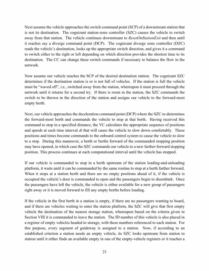
Next assume the vehicle approaches the switch command point (SCP) of a downstream station that is not its destination. The cognizant station-zone controller (SZC) causes the vehicle to switch away from that station. The vehicle continues downstream to ResetOnStationExit and then until it reaches say a diverge command point (DCP). The cognizant diverge zone controller (DZC) reads the vehicle’s destination, looks up the appropriate switch direction, and gives it a command to switch either to the right or left depending on which direction provides the shortest time to its destination. The CC can change these switch commands if necessary to balance the flow in the network. Now assume our vehicle reaches the SCP of the desired destination station. The cognizant SZC determines if the destination station is or is not full of vehicles. If the station is full the vehicle must be “waved off”, i.e., switched away from the station, whereupon it must proceed through the network until it returns for a second try. If there is room in the station, the SZC commands the switch to be thrown in the direction of the station and assigns our vehicle to the forward-most empty berth. Next, our vehicle approaches the deceleration command point (DCP) where the SZC re-determines the forward-most berth and commands the vehicle to stop at that berth. Having received this command to stop in a specified distance, the VC calculates the appropriate sequence of positions and speeds at each time interval dt that will cause the vehicle to slow down comfortably. These positions and times become commands to the onboard control system to cause the vehicle to slow to a stop. During this maneuver, a berth or berths forward of the commanded stopping position may have opened, in which case the SZC commands our vehicle to a new farther-forward stopping position. This process continues at each computational interval until the vehicle has stopped. If our vehicle is commanded to stop in a berth upstream of the station loading-and-unloading platform, it waits until it can be commanded by the same routine to stop at a berth farther forward. When it stops at a station berth and there are no empty positions ahead of it, if the vehicle is occupied the vehicle’s door is commanded to open and the passengers begin to disembark. Once the passengers have left the vehicle, the vehicle is either available for a new group of passengers right away or it is moved forward to fill any empty berths before loading. If the vehicle in the first berth in a station is empty, if there are no passengers wanting to board, and if there are vehicles waiting to enter the station platform, the SZC will give that first empty vehicle the destination of the nearest storage station, whereupon based on the criteria given in Section VIII it is commanded to leave the station. The ID number of this vehicle is also placed in a register of empty vehicles headed to storage, with these numbers referenced to each station. For this purpose, every segment of guideway is assigned to a station. Now, if according to an established criterion a station needs an empty vehicle, its SZC looks upstream from station to station until it either finds an available empty in one of the empty-vehicle registers or it reaches a

22

storage station where an empty vehicle is available. The SZC then simply changes the destination of that empty vehicle to its own, whereupon the vehicle is committed and no longer available to be diverted to another station. The priority in which stations seek empty vehicles is important. During each computation interval, in a routine called SetupCallEmpty the priority is taken in accordance with wait time for stations in which passengers are waiting, longest wait first, then for the remaining stations the order is randomized differently each computational interval. If the wait time at a certain station has become unusually long, its call criterion can be increased so that vehicles can be called sooner. Line speed changes are of two types: 1) due to high winds the line speed must be reduced according to a formula and then increased after the wind dies down, and 2) at specific points in the network where the vehicle must slow down for a curve and then increase speed again after passing the curve. Code for these functions is included in the routines ChangeLineSpeedDueToWind and ChangeLineSpeedAtSpecificPoints. In the latter routine, increasing speed at a specific point has no effect on the vehicles behind, but in decreasing speed, if a vehicle behind is too close, the headway between it and the vehicle ahead may go below the minimum allowable unless it is commanded to the new line speed at the same time, which is done. The criterion for slowing a vehicle down simultaneously with one that has reached the speed-change command point is derived in Reference 11. Converting the above commands into code is a straightforward iterative process that can be appreciated in detail only through the process of writing code. To do it one must simply plunge in. Only then will one appreciate the conditions that arise and that must be corrected though code revision and addition. To catch errors in the developmental program, the primary but not only tool is a Headway Checker, which stops the simulation program if a headway violation is found. It provides enough information so that with the Randomizer off5 the program can be run again and again until the exact cause of the error is found and corrected. Often quite a number of runs are needed to discover the exact cause of the error. While laborious, it is essential that the programmer not guess at a cause of an error. Much more often than not the real cause is not obvious. The present stage of the developmental program is such that hundreds of runs have been made with no error. While laborious and requiring a great deal of patience, the development of the program needed to simulation an ITNS network is a straight-forward application of mathematics, mechanics, and logic, and has been developed by almost every PRT developer (See Reference 9).

5 With the Randomizer off the program generates the same sequence of pseudo-random numbers each time.

23

IV. Hardware & Software Elements

The Control System needed to operate ITNS consists of the following elements.

Hardware:

WHAT HOW

Instruments on board the vehicles to sense speed and position.

Encoders mounted on wheels convert motion into a series of electrical pulses that can be converted into digital information. Since we use the main support wheels only for suspension and not for propulsion and braking, such devices provide accurate information on both distance and speed and are commercially available. Averaging left and right encoder outputs gives the correct position and speed around curves and providing encoders in both front and rear wheels provides redundancy.

Instruments at wayside to separately sense speed and position of vehicles for wayside computers.

The best-known scheme uses magnetic markers, pairs of which permit speed to be measured by measuring the time between closely spaced magnets.

A secure, environmentally friendly communications medium.

Leaky cables are commercially available at low cost and can be mounted inside the guideway to act as the communications medium. There are many suppliers.

Transcevers to transmit and receive information between vehicles and wayside via the leaky cable.

It may be necessary to design these devices from scratch to conform to the specific requirements.

Transducers, i. e., devices that convert information from one type to another – analog to digital, digital to analog.

Commercially available.

Means for propelling and braking the vehicle. Linear induction motors (LIM) driven by variable frequency drives (VFD) provide all-weather operation and are commercially available. A pair of parking and emergency brakes will be provided, in which a high-friction pad presses down on the running surface and is operated by a ball-screw actuator. For parking this brake operates every

24

time the vehicle stops. It is used for emergencies in the rare case that LIM braking is not available.

Means for permitting a vehicle to switch from one guideway to another.

The preferred means has an on-board switch arm that can engage a switch rail on either the left or right side. The guideway has no moving track parts.

Computers to be used in dual duplex sets. Commercially available.

Software:

Software to convert information from sensors to digital information.

Commercially available.

Software to convert information from digital to voltages and frequencies.

Commercially available.

Software in vehicle computers to cause the vehicle door to open or close.

Commercially available, e. g. for operating elevator doors.

Software in vehicle computers required to operate the heating, ventilating, and air conditioning equipment.

Commercially available.

Software in vehicle computers required for calculating speed and position commands, comparing them with actual speeds and positions, multiplying them by suitable gain constants, and outputing commands to analog devices.

Commonly known to control engineers. See paper “Longitudinal Control of a Vehicle.”

Vehicle software that corrects for step changes in position due to encoder calibration without the controller seeing a step change in position.

When the encoder must be calibrated, the same correction must be fed into the command position.

Software in each wayside computer to receive speed-and-position information separately from each vehicle in its domain, to verify that that information is correct, and to take corrective information if not.

This is the monitoring and safety function of the zone controller.

Software in each wayside computer to interpret the position and speed of each

The methods are described in open literature and the needed code has been developed.

25

vehicle in its domain and to send the appropriate maneuver command when needed to a specific vehicle. Different software is needed in station zone controllers, merge zone controllers, and diverge controllers.

Software in a central computer to calculate the switch table needed in diverge-zone controllers and to adjust it for traffic conditions.

This is a straightforward process using known methods.

Software to permit wayside diverge-point computers to command vehicles to switch left or right based on transmitted knowledge of the destination.

When a vehicle reaches a diverge command point, the cognizant wayside computer interrogates the vehicle for its destination, looks up in a switch table the right or left switch command for that destination, and transmits it to the vehicle.

Software to permit wayside merge-point computers to command vehicles to slip when necessary to maintain pre-set minimum headway.

When a vehicle reaches a merge command point, the wayside ZC for that merge checks the positon of vehicles on the other branch and commands slip when needed. These actions have been programmed.

Software to permit speed to be changed in different parts of a network, to reduce speed in high wind conditions, and to increase it again when the wind dies down.

This process has been programmed.

Software in wayside computers called “zone controllers” to permit one zone controller to pass vehicles to the next zone controller.

A straightforward programming task.

Software in wayside zone controllers to pass status information from vehicles to a central computer.

A straightforward programming task.

Software in a central computer to assist the optimum movement of empty vehicles.

The method we have programmed is described in Reference 9.

Software in a central computer to gather, interpret, and display performance data.

A straightforward programming task.

Software to enable voice communication between vehicles and a wayside control room.

This has not yet been programmed.

26

V. The System Software Elements Some of this information has been given in a different form. 5.1. Control of a Vehicle

• Inputs from wayside Zone Controller:

Speed every Time Multiplexing Interval. Maneuver command at Command Points. Switch commands before every diverge and merge.

• Input from on-board Encoder: Distance-pulse stream

• At fixed intervals along the guideway, update vehicle position and correct speed.

• As a vehicle leaves a station, calibrate the position signal.

• Calculate: Command Acceleration(t)

Command Speed(t) Command Position(t) Measured distance, from encoder Measured speed, from distance and time encoder increments Command Thrust using calculated gains Switch Position

• Outputs: Voltage Frequency Switch command 5.2. Control of a Station Zone (SZC)

• The domain of the SZC is from the closest upstream branch point (BP), which may be a line-to-line BP or the nearest upstream guideway diverge point to the cognizant station output diverge point.

• Every Time Multiplexing Interval (TMI) the SZC sends the line speed to all vehicles in its domain, and receives from each vehicle in its domain its speed and position measured from the nearest downstream line-to-line BP.

• The SZC calculates the expected speed and position of each vehicle in its domain and

removes the speed signal if the values from a vehicle are outside an agreed range.

• Every TMI the SZC is informed of a vehicle in the upstream zone that will arrive in its domain in the next TMI and so informs the downstream zone of the same.

27

• When a vehicle reaches the station’s switch command point (SCP), the SZC determines if

it is to switch into the station and if so, assigns it the forward-most empty berth.

• When a vehicle commanded to switch into the station reaches the station’s deceleration command point (DCP) the SZC reassigns it to the forward-most empty berth, which may have changed, and commands it to stop in the distance to that berth.

• When a vehicle is either decelerating into the station or stopped and a berth further

forward becomes empty, the SZC commands the vehicle to stop at the new forward-most available berth. The vehicle’s door must be closed in order for it to accept the command to move forward.

• When a vehicle is assigned to the first berth, whether in it or moving to it, the SZC, with

knowledge of the positions of all vehicles on the main line guideway, determines when to command the vehicle to line speed. See Section VIII.

5.3 Control of Merging (MZC)

• The domain of the MZC is from the downstream guideway junction (the merge point) upstream on each leg to the nearest BP.

• Every TMI the MZC sends the line speed to all vehicles in its domain, and receives from each vehicle in its domain its speed and position measured from the merge point ahead.

• The MZC calculates the expected speed and position of each vehicle and removes the speed signal if these values are outside an agreed range.

• Every TMI the MZC is informed of the position, speed, and acceleration of a vehicle in

the upstream zone on either leg that will arrive in its domain in the next TMI and so informs the downstream zone of the same.

• When a vehicle just passes the merge command point (MCP), the MZC determines if the vehicle upstream of and closest to MCP on the other leg is close enough to violate the minimum-headway criterion. If so, this vehicle is commanded to slip back enough to maintain the set minimum headway, and simultaneously any vehicle upstream of it that would violate set minimum headway is commanded to slip. This process continues until no further slipping is needed. The program is designed to slip vehicles upstream of the upstream station and line BPs if necessary.

28

5.4. Control of Diverging (DZC)

• The domain of the DZC is from the downstream guideway junction (the diverge point) upstream to the nearest station or line BP,

• Every TMI the DZC sends the line speed to all vehicles in its domain and receives from each vehicle in its domain its speed and position measured from the diverge point ahead.

• The DZC calculates the expected speed and position of each vehicle and removes the speed signal if these values do not agree within a set range of the values transmitted from the vehicle.

• Every TMI the DZC is informed of the kinematic properties of a vehicle in the upstream

zone that will arrive in its domain in the next TMI and so informs the downstream zones of the same.

• The DZC maintains a switch table, which is a table of switch commands to each station

in the system. This table may be revised by commands from the central controller.

• When a vehicle reaches the diverge command point (DCP) the DZC requests its destination, looks up the corresponding switch command (left or right), and sends the switch command to the vehicle.

5.5. Central Control (CC)

• The CC communicates only with the zone controllers. Each ZC communicates with both the CC and the VC in its domain.

• The CC receives and processes data received from each ZC. This includes trip length, energy use, wait time, ride time, and expected ride time.

• The CC updates a calculation of system dependability6 each TMI. • The CC obtains data from the ZCs each TMI on the positions and speeds of all of the

vehicles and determines, based on traffic, when to change certain commands in the switch tables of certain SZCs.

5.6 Empty-Vehicle Movement

• When a station has a surplus empty vehicle in or approaching its first berth, based on a criterion given elsewhere, the cognizant SZC gives it the destination of the nearest

6 "Dependability as a Measure of On-Time Performance of Personal Rapid Transit Systems," JAT, 26:3(1992):101-212.

29

storage station and simultaneously enters the number of this empty vehicle into a register corresponding to the station.

• As the empty vehicle moves from zone to zone, its number is transferred to a register corresponding to the zone it is in.

• When a station needs an extra empty vehicle, based on a given criterion, its SZC looks upstream from ZC to ZC in order of proximity on all branches for the nearest available empty vehicle, i.e., one in an empty-vehicle register. When one is found, its destination is changed to that of the station in need.

• The order of priority of the search for empties is important. The order is that of the station with the longest wait time, the second longest, and so on until stations with no empty vehicles are reached. For them the order is random, with the random order changed every computational interval.

• The criterion for needing an empty is when the number of vehicles in a station is below n m+ where n is the number of station berths (where unloading and loading can take place), and m is a number (a call criterion) that can be changed by the operator or by the CC based on the observed wait times at each station, in order to decrease the difference between average wait times at all stations.

• The system average wait time can be decreased by adding more vehicles.

VI. The Command Points and Actions

Equations need to be incorporated into the program for the following command points.

6.1. Switch Command Point (SCP)

The SCP is located far enough upstream of the diverge point into the station so that if the vehicle failed to detect that the switch is in one of the two locked positions, the vehicle would be able to stop before hitting the diverge junction. This distance is at least

𝐷𝐷𝑆𝑆𝑆𝑆𝑆𝑆 = 𝑉𝑉𝐿𝐿𝑡𝑡𝑠𝑠𝑠𝑠𝑠𝑠 +𝑉𝑉𝐿𝐿2

2𝑎𝑎𝑒𝑒

in which VL is the line speed, tswx is the time required for the switch to throw and be detected, and ae is the emergency deceleration.

6.2. Deceleration Command Point

As shown in the paper “Guideway Geometry”, we have found that to reduce the length of the offline guideway we can and should initiate deceleration into a station before the vehicle completely clears the main line. In so doing, the bypass line length can be reduced a large amount while sacrificing as little as 0.1 second on-line headway. The position of the DCP can be approximated as follows: The length of the transition curve from the main line to the parallel by-pass line is very close to

30

1/3

42 2

L stat

c

V V HLJ

+ =

in which

line speedlimit speed through stationcenterline separation between mainline and bypass linecomfort value of lateral jerk, 0.25g/s

L

sta

c

VVHJ

====

The stopping distance of a vehicle is

2

cL Lstop

c c

AV VDA J

= +

Thus, we can approximately set the DCP upstream of the diverge junction into the station by the amount

.DCP stop tD D L= −

At low line speeds this quantity may be negative.

The quantity 𝐷𝐷𝑆𝑆𝑆𝑆𝑆𝑆 must be greater than 𝐷𝐷𝐷𝐷𝑆𝑆𝑆𝑆 + 𝑉𝑉𝐿𝐿 × 𝑡𝑡𝑠𝑠𝑠𝑠𝑠𝑠.

6.3. Diverge Command Point

Set the DCP upstream of each line-to-line diverge junction by the amount

2

2L

DCP L swx flare tolerancee

VD V t D Da

= + + +

Where Dflare is the distance from the diverge junction to the end of the switch rail.

6.4. Merge Command Point

The merge command point must be place upstream of each line-to-line merge junction point by the amount

MCP slip clearance toleranceD D D D= + +

in which slipD is the distance traveled by a vehicle slipping two headway7 distances ,L hV t in which

ht is the line headway. clearanceD is the distance from the merge junction point upstream to the point

7 Further simulation work may increase this value.

31

where a pair of vehicles on opposite branches approaching at equal distances from the junction point would just touch, and toleranceD is a suitable safety distance.

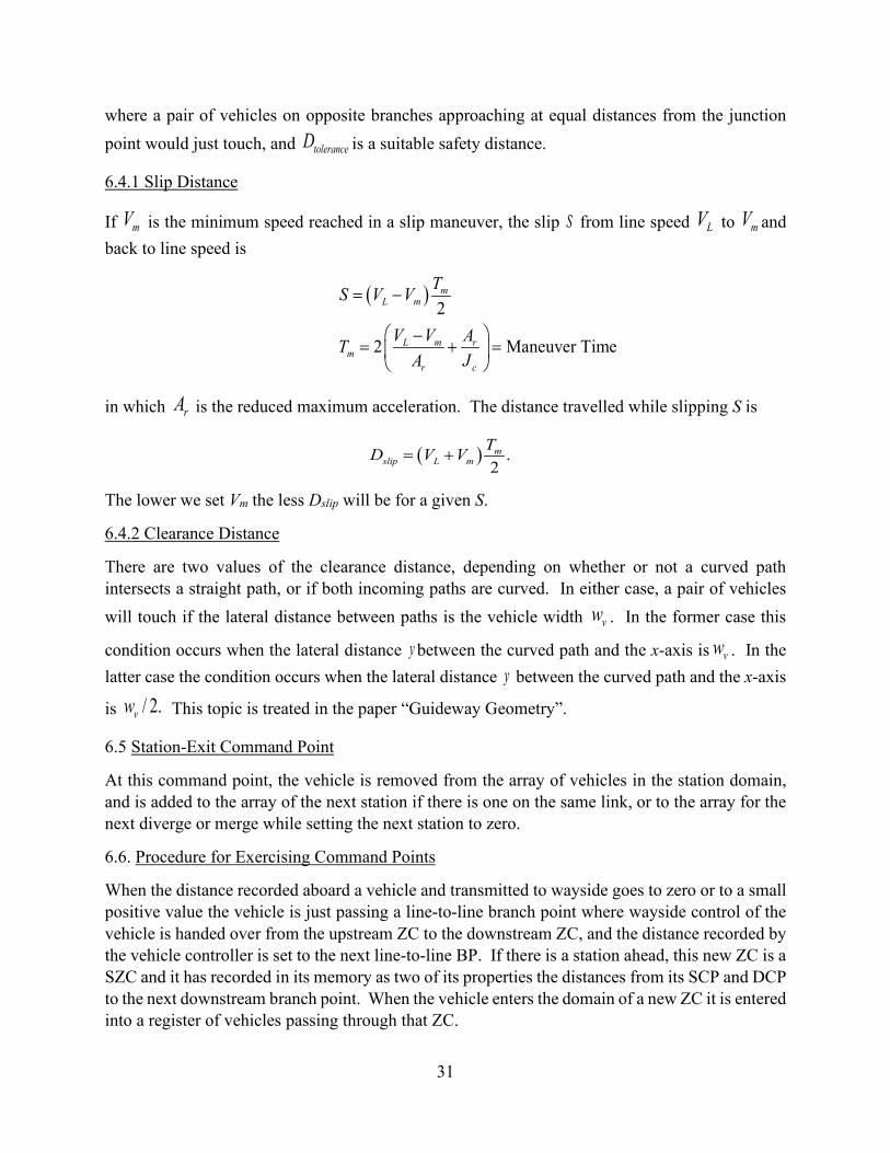
6.4.1 Slip Distance

If mV is the minimum speed reached in a slip maneuver, the slip S from line speed LV to mV and back to line speed is

( )

2

2 Maneuver Time

mL m

L m rm

r c

TS V V

V V ATA J

= −

−= + =

in which rA is the reduced maximum acceleration. The distance travelled while slipping S is

( ) .2m

slip L mTD V V= +

The lower we set Vm the less Dslip will be for a given S.

6.4.2 Clearance Distance

There are two values of the clearance distance, depending on whether or not a curved path intersects a straight path, or if both incoming paths are curved. In either case, a pair of vehicles will touch if the lateral distance between paths is the vehicle width vw . In the former case this

condition occurs when the lateral distance y between the curved path and the x-axis is vw . In the latter case the condition occurs when the lateral distance y between the curved path and the x-axis

is / 2.vw This topic is treated in the paper “Guideway Geometry”.

6.5 Station-Exit Command Point

At this command point, the vehicle is removed from the array of vehicles in the station domain, and is added to the array of the next station if there is one on the same link, or to the array for the next diverge or merge while setting the next station to zero.

6.6. Procedure for Exercising Command Points

When the distance recorded aboard a vehicle and transmitted to wayside goes to zero or to a small positive value the vehicle is just passing a line-to-line branch point where wayside control of the vehicle is handed over from the upstream ZC to the downstream ZC, and the distance recorded by the vehicle controller is set to the next line-to-line BP. If there is a station ahead, this new ZC is a SZC and it has recorded in its memory as two of its properties the distances from its SCP and DCP to the next downstream branch point. When the vehicle enters the domain of a new ZC it is entered into a register of vehicles passing through that ZC.

32

When a vehicle reaches a SCP the SZC evokes a subroutine that determines if it is to switch into the station based on the destination of the vehicle and the occupancy of the farthest upstream waiting berth. If it is to switch into the station, the SZC commands the vehicle’s switch to be thrown, assigns it to the forward-most empty berth, and records that the SCP function for that vehicle has been evoked. (The berth assignment is recorded both in the SZC and in the vehicle computer.) Completion of the SCP function can be indicated by dividing the SZC’s register of vehicles into two sub-registers: one for those that are upstream of the SCP or downstream of it and committed to bypass the station, and a second for those that are downstream of the SCP and are committed to enter the station.

When a vehicle reaches a deceleration command point (DCP) and the vehicle is to enter the station, the SZC evokes a subroutine that updates the forward-most berth assignment and commands the vehicle to stop at that forward-most berth.

When a vehicle reaches the downstream merge point of the mainline and bypass line out of a station, it is passed off to either the SZC for the next station on the same link, or to either a DZC or a MZC for the same link. In either case the vehicle is removed from the register of the upstream ZC and simultaneously entered into the register of the downstream ZC.

If the downstream line-to-line branch point is a diverge, when the vehicle reaches its DCP it is interrogated for its destination, the DZC finds the appropriate switch command from its stored switch table and sends it to the vehicle controller, whereupon the VC commands its switch to be thrown if it is in the wrong direction.

If the downstream line-to-line branch point is a merge, when the vehicle reaches its MCP the cognizant MZC determines if it will be in conflict with a vehicle on the other branch of the merge and if so causes vehicles to slip back as described in the paper “Transitions.”

VII. Test for a Headway Violation upon Decelerating into a Station 7.1 Kinematics of two successive vehicles moving into a station.

Consider a vehicle #1 decelerating into a station to station speed staV and then to rest followed by

a vehicle #2 a time hT behind undergoing exactly the same maneuver. Let the position of vehicle #1 at time zero be (0) 0.x = The times, accelerations, speeds, and positions of vehicle #1 at the points 1, 2, 3, 4, 5, 6, and 7 in Figure 7.1, following the methodology of the paper “Transitions,” are as follows:

33

Figure 7.1. The velocity profiles of a pair of vehicles entering a station.

( )21 1

1 1 101 1 01 01 01 01

1 1 123 2 23 23 23 2 23

1 212 12 12 1 12

34 34

45

if / then else

, ,2 6

, ,2 3

,2

/

L sta c c c c L sta

L Lc

stac

c

c

sta

c

V V A J A A A J V V

A A Adt V V dt dx dt V dtJA A Adt V V dt dx dt V dtJ

AV Vdt dx dt V dtA

dt dx VAdt

− ≥ = = −

= = − = −

= = + = −

− = = −

=

= 5 45 45 45 45

67 6 67 67 67 6 67

5 656 56 56 5 56

, ,2 6

, ,2 3

,2

c csta sta

c

c c c

c

c

c

A AV V dt dx dt V dtJA A Adt V dt dx dt V dtJV V Adt dx dt V dt

A

= − = −

= = = −

− = = −

(7-1)

𝑡𝑡1 = 𝑑𝑑𝑡𝑡01, 𝑡𝑡2 = 𝑡𝑡1 + 𝑑𝑑𝑡𝑡12, 𝑡𝑡3 = 𝑡𝑡2 + 𝑑𝑑𝑡𝑡23, 𝑡𝑡4 = 𝑡𝑡3 + 𝑑𝑑𝑡𝑡34 (7.2) 𝑡𝑡5 = 𝑡𝑡4 + 𝑑𝑑𝑡𝑡45, 𝑡𝑡6 = 𝑡𝑡5 + 𝑑𝑑𝑡𝑡56, 𝑡𝑡7 = 𝑡𝑡6 + 𝑑𝑑𝑡𝑡67 (7.3)

𝑥𝑥1 = 𝑑𝑑𝑥𝑥01, 𝑥𝑥2 = 𝑥𝑥1 + 𝑑𝑑𝑥𝑥12, 𝑥𝑥3 = 𝑥𝑥2 + 𝑑𝑑𝑥𝑥23, 𝑥𝑥4 = 𝑥𝑥3 + 𝑑𝑑𝑥𝑥34 (7.4) 𝑥𝑥5 = 𝑥𝑥4 + 𝑑𝑑𝑥𝑥45, 𝑥𝑥6 = 𝑥𝑥5 + 𝑑𝑑𝑥𝑥56, 𝑥𝑥7 = 𝑥𝑥6 + 𝑑𝑑𝑥𝑥67 (7.5)

Using the above canonical formulation, the acceleration, speed, and position of vehicle 1 at any value of t are as follows:

34

( )

1

1 2 1 1 1 1

12 3 2 1 2 2 2

3 4 3 3

4

0 : , , ,2 6

: , , ,2

: , , ,2 3

: , 0, ,

c L L

c

c

sta sta

A At t t t A J t V V t x t V t

At t t t t t A A V V tA x x t V t

A A At t t t t t A A J t V V t x x t V t

t t t t t t A V V x x V t

t

≤ ≤ ∆ = = − ∆ = + ∆ = ∆ + ∆

≤ ≤ ∆ = − = − = + ∆ = + ∆ + ∆

− + ≤ ≤ ∆ = − = − + ∆ = + ∆ = + ∆ + ∆

≤ ≤ ∆ = − = = = + ∆

≤

( )

5 4

5 6 5 5 5 5

6 7 6 6 6 6

: , , ,2 6

: , , ,2

: , , ,2 3

c sta sta

c

cc c

A At t t t t A J t V V t x t V t

At t t t t t A A V V tA x x t V t

A A At t t t t t A A J t V V t x x t V t

≤ ∆ = − = − ∆ = + ∆ = ∆ + ∆ ≤ ≤ ∆ = − = − = + ∆ = + ∆ + ∆

− + ≤ ≤ ∆ = − = − + ∆ = + ∆ = + ∆ + ∆

(7-

6)

For vehicle #2 up to time ht T= the speed stays constant at LV and the distance traveled is

Lx V t= . For ht T> we can obtain the acceleration, speed, and position as functions of time by

substituting ' forht t T t= − in equations (7-6). 7.2 Results

Some results of a program to calculate the kinematics of Section 7.1 are given in Figures 7.2 and 7.3. Note from Figure 7.3 that in the case shown the small headway violation increases from zero back to zero in about one second. If based on criteria used, it is judged that the minimum headway between these two vehicles will be too small, vehicle #2 will have to be slipped back an amount that can be readily determined.

35

Figure 7.2. Kinematics of a pair of vehicles decelerating to station speed.

Figure 7.3. Separation and minimum allowable separation between two vehicles entering a station.

0 1 2 3 4

TIME, seconds

0

1

2

3

4

5

6

7

8

9

10

11

12

13

Actua

l and

mini

mum

sepa

ratio

ns, m

eters

Separation between veh 1 and 2Minimum allowable separation

0 1 2 3 4

TIME, seconds

-10

0

10

20

30

40

Acce

lerati

on, s

peed

, and

dista

nce t

rave

lled i

n MKS

units Acceleration of veh 1

Speed of veh 1Distance veh 1 has traveledAcceleration of veh 2Speed of veh 2Distance veh2 has traveled

36

VIII. Boundaries of the Forbidden Zone When the Subroutine CommandLineSpeed determines that the vehicle in the first birth (here called Veh) has been given a destination and loading of passengers is complete, it runs the Subroutine setSpeedChangeManeuver. This routine calculates the maneuver time and distance, Tm and Dm, respectively. At this point, it is necessary to determine if any vehicles on the line bypassing the station would conflict if Veh would be dispatched at this instant. Veh may be at any speed less than the station speed and any acceleration within comfort limits. It follows a curved path such as the heavy line in Figure 8.1, which begins at zero time and zero distance. When the maneuver is finished, it is at the time Tm and distance Dm. A vehicle bypassing the station at line speed VL that would also arrive at the time Tm and distance Dm would at time zero be at distance 𝑉𝑉𝐿𝐿𝑇𝑇𝑚𝑚 − 𝐷𝐷𝑚𝑚 upstream of the position of Veh. If the minimum time headway is Th then any vehicle bypassing the station within a distance of 𝑉𝑉𝐿𝐿𝑇𝑇ℎ of the distance 𝑉𝑉𝐿𝐿𝑇𝑇𝑚𝑚 − 𝐷𝐷𝑚𝑚 at time 0 will be in the FORBIDDEN ZONE as shown by the red line in Figure 8.1. If the position of Veh behind the branch point ahead is P, then the boundaries of the FORBIDDEN ZONE are

𝐵𝐵𝐵𝐵𝐵𝐵𝐵𝐵𝑑𝑑𝑎𝑎𝐵𝐵𝐵𝐵𝐵𝐵ℎ𝑒𝑒𝑎𝑎𝑑𝑑 = 𝑃𝑃 − (𝑉𝑉𝐿𝐿𝑇𝑇𝑚𝑚 − 𝐷𝐷𝑚𝑚) + 𝑉𝑉𝐿𝐿(𝑇𝑇ℎ + 𝑐𝑐_𝑑𝑑𝑡𝑡) 𝐵𝐵𝐵𝐵𝐵𝐵𝐵𝐵𝑑𝑑𝑎𝑎𝐵𝐵𝐵𝐵𝐵𝐵𝑒𝑒ℎ𝑖𝑖𝐵𝐵𝑑𝑑 = 𝑃𝑃 − (𝑉𝑉𝐿𝐿𝑇𝑇𝑚𝑚 − 𝐷𝐷𝑚𝑚) − 𝑉𝑉𝐿𝐿(𝑇𝑇ℎ + 𝑐𝑐_𝑑𝑑𝑡𝑡)

in which 𝑐𝑐_𝑑𝑑𝑡𝑡 is the computation interval.

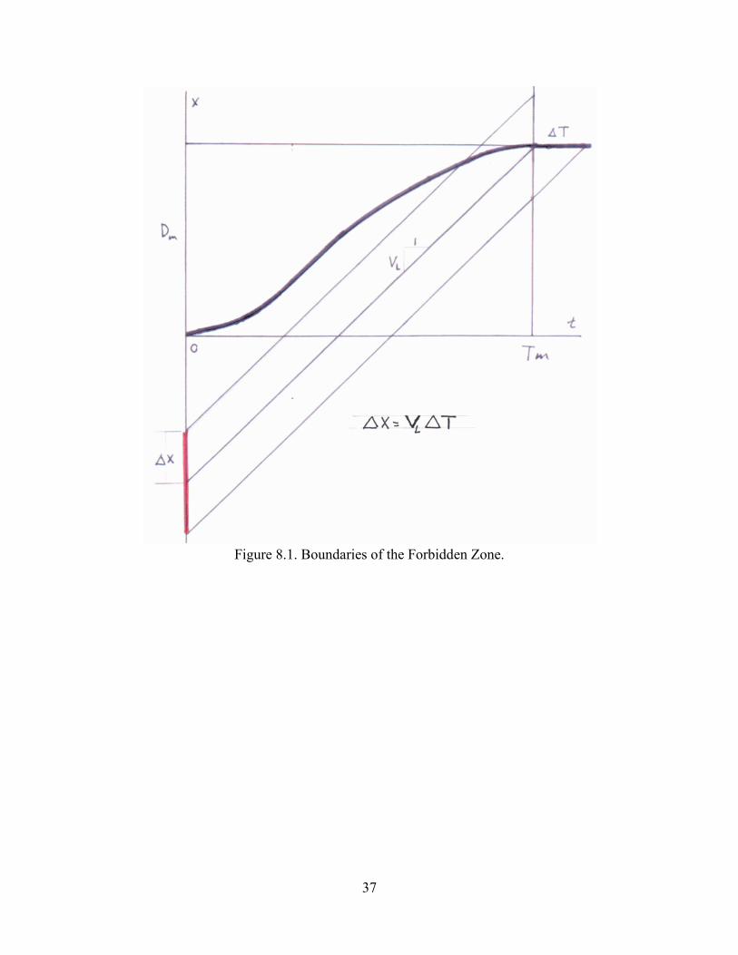
37

Figure 8.1. Boundaries of the Forbidden Zone.

38

Controlling many Vehicles in ITNS The control system consists of computers, sensors, and a communications medium.

Computers

All computers in the system are dual redundant, which means that each “computer” is really two pairs of computers. The output of the computers in each pair is compared 20 times a second, and likewise the common output of the two pairs is compared 20 times a second. Any error detected causes the vehicle to be directed to a maintenance shop directly upon completing its trip. With this arrangement the mean time between serious events is extremely long, longer than would be believed without checking the calculations. See the internal paper “Failure Modes and Effects.”

There are three types of computers: vehicle computers, wayside computers, and a central computer. Each section of guideway is managed by a wayside computer called a zone controller. There will be station zones, merge zones, diverge zones, and line zones. The zone controllers command specific maneuvers to specific vehicles and the vehicle computers respond to these commands. We have worked out the algebra needed to command every maneuver required, which consist of maneuvering from a station to line speed, slipping a certain distance ahead of merge points, and stopping in a given distance. With today’s high-gain controllers we control the position of a vehicle almost as closely as we can measure it.

Each zone controller provides the line-speed signal in its domain. If anything goes wrong, it removes the speed signal, which causes the vehicles to slow to creep speed. When a vehicle reaches a maneuver-command point, the zone controller transmits the appropriate command maneuver to that vehicle, and the vehicle controller causes the vehicle to follow the required time sequence of positions and speeds. The zone controller calculates the same maneuver sequentially for each vehicle in its domain and compares it with the vehicle’s position and speed. If it detects an anomaly it removes the speed signal from its portion of the guideway, which causes the vehicles to slow to creep speed. Adjacent zone controllers communicate with each other.

The central computer balances traffic in certain conditions and accumulates data on the performance of the system.

The data rates, computer speeds, and memory needed are well within the capability of today’s computers.

On-Board Position and Speed Sensing

The position and speed of each vehicle is measured on board each vehicle by means of digital encoders placed in the main bearing of each of the four wheels. Averaging the left and right output gives the correct measurement in curves. Having encoders in both the fore and aft wheels provides redundancy. These encoders register at least 4096 pulses per revolution, or with the 13.25” OD tires we plan to use, about 0.010” per pulse. With this accuracy, experimental evidence has shown that we can differentiate to obtain accurate speed measurements. If the assumed the OD was in error by say 1%, the distance measurement would be in error by 1%. Thus, we will calibrate each vehicle as it leaves a station by means of fixed magnetic markers. In this way we will know the position of each vehicle to an accuracy of less than one inch.

Wayside Position and Speed Sensing

The position and speed of each vehicle is measured by suitably placed pairs of wayside markers. When a vehicle reaches the first marker, a pulse sent to the cognizant wayside computer, which detects its position

39

at that time. When the vehicle reaches the second of the pair a known and short distance ahead, measuring the time interval between markers determines speed.

Communication

Each vehicle will be equipped with a transmitter and a receiver capable of sending information to and receiving information from a leaky cable placed on the inside of the guideway. The zone controllers similarly talk to and from the cable. Such cables are commercially available. This type of communication is completely secure and cannot be interfered with by hackers.

Background and Conclusions

Many engineers have been working on controlling PRT vehicles since the 1960s. We have followed this work closely and during our PRT Design Study for the Chicago RTA (1991-94) my team worked with experienced engineers from Raytheon and Hughes on the details. We have continued to refine the control system and the simulation of PRT systems so that today we are extremely confident that the system will work as we predict. Computer memory has doubled every 18 months since the 1960s so the computers needed today to handle the requirements are very small and extremely fast. With the use of dual redundancy failures that may occur in the system will not be due to the computers.

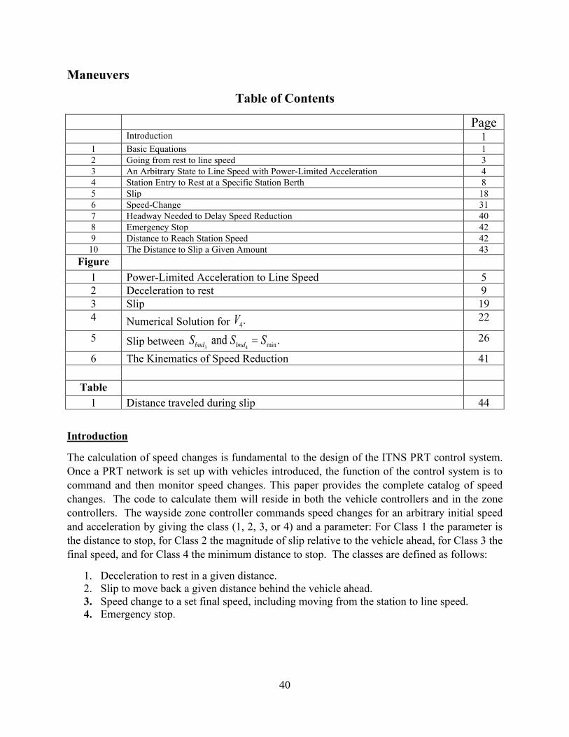
40

Maneuvers

Table of Contents

Page Introduction 1

1 Basic Equations 1 2 Going from rest to line speed 3 3 An Arbitrary State to Line Speed with Power-Limited Acceleration 4 4 Station Entry to Rest at a Specific Station Berth 8 5 Slip 18 6 Speed-Change 31 7 Headway Needed to Delay Speed Reduction 40 8 Emergency Stop 42 9 Distance to Reach Station Speed 42

10 The Distance to Slip a Given Amount 43 Figure

1 Power-Limited Acceleration to Line Speed 5 2 Deceleration to rest 9 3 Slip 19 4 Numerical Solution for 4.V 22

5 Slip between 3 4 min and .bnd bndS S S= 26

6 The Kinematics of Speed Reduction 41

Table 1 Distance traveled during slip 44

Introduction

The calculation of speed changes is fundamental to the design of the ITNS PRT control system. Once a PRT network is set up with vehicles introduced, the function of the control system is to command and then monitor speed changes. This paper provides the complete catalog of speed changes. The code to calculate them will reside in both the vehicle controllers and in the zone controllers. The wayside zone controller commands speed changes for an arbitrary initial speed and acceleration by giving the class (1, 2, 3, or 4) and a parameter: For Class 1 the parameter is the distance to stop, for Class 2 the magnitude of slip relative to the vehicle ahead, for Class 3 the final speed, and for Class 4 the minimum distance to stop. The classes are defined as follows:

1. Deceleration to rest in a given distance. 2. Slip to move back a given distance behind the vehicle ahead. 3. Speed change to a set final speed, including moving from the station to line speed. 4. Emergency stop.

41

All these speed changes start from given speed and acceleration. Since a very high-gain controller is use on board based on position and speed,8 the initial speed and acceleration used on board the vehicle to command speed changes are the command values. The actual speed and position will differ by only a small amount. The complete set of speed changes derived here are all performed in minimum time consistent with given ride comfort values of acceleration and jerk.

In Section 1, the equations for going from rest to line speed are derived. In Section 2 these equations are applied, as an example, to the simplest transition from rest to line speed. In Section 3, the power-limited transition from arbitrary initial speed and acceleration to line speed is derived. This transition is included in the set derived in Section 6. Section 4 derives Class 1. Section 5 derives Class 2, Section 6 derives Class 3, and next is the derivation of Class 4.

1. Basic Transition Equations

The transitions are driven by constant jerk, at the comfort level or below. With this assumption consider the motion of a vehicle. J is the constant jerk, A is acceleration, V is speed, and x is the distance traveled. Then

2 2 3

0 0 0 0 0 0, , ,2 2 6t t tx J x A Jt x V A t J x x V t A J= = + = + + = + + +&&& && & (1-1)

Consider a transition from point 0 to point 1. Call the time interval from 0 to 1 01dt . Then

( ) ( )

( )

( )

1 001

01 01 0 11 0 0 0 0 1 0 0 01

1 001

0 1

01 0 101 01 0 0 01 01 0 01

2 22 2 2

/ 2

236 6

A AdtJdt dt A AV V A Jdt V A A A V dt

V VdtA A

dt A Adx dt V A Jdt dt V dt

−=

+ = + + = + + − = +

−=

+

+ = + + = +

(1-2)

So, in words, the time interval is the increase in acceleration divided by positive jerk, or the decrease in acceleration divided by negative jerk, or the increase in speed divided by the average acceleration. The new speed is the old speed plus the average acceleration multiplied by the time interval, and the increase in distance is the time interval multiplied by a quantity consisting of the old speed plus the time interval times one sixth the quantity twice the old acceleration plus the new acceleration. These simple rules are all that are needed to derive any transition.9

8 J. E. Anderson, "Longitudinal Control of a Vehicle," JAT, 31:3(1997):237-247. 9 These rules were, to my knowledge, first derived by Raytheon control engineer Richard Radnor.

42

2. Basic Transition from rest to line speed

We start the transition by applying the comfort level of jerk, cJ until the acceleration reaches the

comfort level cA . We then increase speed at this constant acceleration until we approach the

desired speed LV . If we were to continue to line speed and then suddenly reduce acceleration to zero, the passengers would experience infinite jerk, so to stay within comfort jerk, we must at a certain point gradually reduce the acceleration to zero at the rate .cJ− Thus, like all Gaul, the

transition is divided into three parts: part 0 to 1 at constant cJ until ,cA A= part 1 to 2 at constant

cA , and part 2 to 3 at constant cJ− , which ends when 0A = and .LV V= So we can write

( )( ) ( )

201 1 01 01 01

23 2 23 23 23 2 23

12 2 1 12 12 1 12

/ , / 2, / 6/ / , / 2, / 3

/ , / 2

c c c c

c c c c L c c

c c

dt A J V dt A dx dt Adt A J A J V V dt A dx dt V dt A

dt V V A dx dt V dt A

= = =

= − − = = + = +

= − = +

(2-1)

Note that the second row must be calculated before the third row because the speed 2V is not known until the second row is calculated. From the first and middle of the second set of equations

2

2 2c

Lc

AV VJ

= −

Then, using all three sets of equations (2-1) the time from rest to line speed is

2 2

03 01 12 2312

2 2c c c cL

Lc c c c c c

A A A AVdt dt dt dt VJ A J J A J

= + + = + − − = +

(2-2)

The distance from rest to line speed is

( ) ( )

( )

3 2 22 1

03 01 12 23 1 2 12

2 22 2 2 2 22 1 2

23

26 2 2 3

1 12 2 2 2 2

if .2

c c c cL

c c c c c

c c c c cL L L L

c c c c c c c c

c cL L LL

c c c c

V VA A A Adx dx dx dx V V V VJ A J J J

V V A A A A AV V V VA J A J J A J J

A AV V V VA J J J

− = + + = + + − + − +

− = + = − + − +

= + = <

(2-3)

So the distance from rest to line speed is simply half the line speed multiplied by the time to line speed, which if graphed shows the symmetry of the transition.

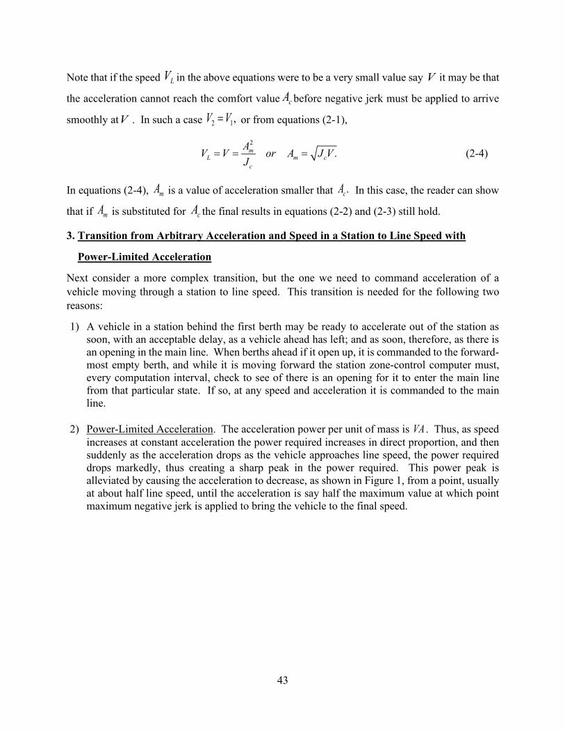
43

Note that if the speed LV in the above equations were to be a very small value say V it may be that

the acceleration cannot reach the comfort value cA before negative jerk must be applied to arrive

smoothly atV . In such a case 2 1,V V= or from equations (2-1),

2

.mL m c

c

AV V or A J VJ

= = = (2-4)

In equations (2-4), mA is a value of acceleration smaller that .cA In this case, the reader can show

that if mA is substituted for cA the final results in equations (2-2) and (2-3) still hold.

3. Transition from Arbitrary Acceleration and Speed in a Station to Line Speed with

Power-Limited Acceleration

Next consider a more complex transition, but the one we need to command acceleration of a vehicle moving through a station to line speed. This transition is needed for the following two reasons:

1) A vehicle in a station behind the first berth may be ready to accelerate out of the station as soon, with an acceptable delay, as a vehicle ahead has left; and as soon, therefore, as there is an opening in the main line. When berths ahead if it open up, it is commanded to the forward-most empty berth, and while it is moving forward the station zone-control computer must, every computation interval, check to see of there is an opening for it to enter the main line from that particular state. If so, at any speed and acceleration it is commanded to the main line.

2) Power-Limited Acceleration. The acceleration power per unit of mass is VA . Thus, as speed increases at constant acceleration the power required increases in direct proportion, and then suddenly as the acceleration drops as the vehicle approaches line speed, the power required drops markedly, thus creating a sharp peak in the power required. This power peak is alleviated by causing the acceleration to decrease, as shown in Figure 1, from a point, usually at about half line speed, until the acceleration is say half the maximum value at which point maximum negative jerk is applied to bring the vehicle to the final speed.

44

Figure 1. Power limited acceleration to line speed.

So, start the transition with 0 0,A V different from zero. Apply positive jerk until maximum acceleration is reached at point 1. Then continue at maximum acceleration to a point 2 where negative jerk is applied until a point 3 is reached, where maximum negative jerk is applied until the acceleration is zero at a final speed at point 4. With this transition we have the following equations:

0 0 001 1 0 01 01 01 0 01

2 12 1 12 12 12 1 12 2

3 3 323 3 2 23 23 23 2 23 3

2, ,2 6

, , ,2

2, , ,2 6

c c c

c

cc L

c

c c cc

n

A A A A A Adt V V dt dx dt V dtJ

V V AA A A dt dx dt V dt V VA

A A A A A Adt V V dt dx dt V dt A AJ

dt

α

β

− + + = = + = + − = = = = + =

− + + = = + = + = −

3 3 3 334 4 3 34 34 34 3 34

0 0 2 0, ,2 6L

c c

A A A AV V V dt dx dt V dtJ J− + + = = = = + = + −

(3-1)

01 12 23 34 01 12 23 34,m mT dt dt dt dt D dx dx dx dx= + + + = + + +

Now with 3A and 2V known, from the fourth row of equations (3-1) we can solve for 3.V Thus

33 34 .

2LAV V dt= − (3-2)

From the second and then the first equation in the third row, we have

( )3 2 323

3 23

2, c

nc

V V A Adt JA A dt

− −= =

+ (3-3)

0 1 2 3 4 5 6 7 8 9 10

TIME, sec

-5

0

5

10

15

20

Units

are

met

ers

& se

cond

s

JerkAccelerationSpeedDistance traveledAcceleration Power/Mass

Power-Limited Acceleration to Line Speed

45

Case when 1 .LV Vα> When 1 LV Vα≤ point 1 is defined as the point where 1 .cA A= But the

power-limited condition is determined by reducing 1A above 2 .LV Vα= Indeed, when

3 3, .cV V A A Aβ= = = Thus we must reduce 1A when 1 LV Vα> linearly from cA when 1 LV Vα=

to 3 cA Aβ= when 1 3V V= . Thus, when 1 2 LV V Vα> = let

( )1 1c LA A m V Vα= − − (3-4)

where

3

(1 ) .c

L

AmV V

βα−

=−

(3-5)

From the first of equations (3-1) we have a second equation relating 1 1and ,A V namely

2 2

1 01 0 .

2 c

A AV VJ−

= + (3-6)

If we substitute 1V from equation (3-6) into equation (3-4), the result can be reduced to the

following quadratic equation for 1.A

21 12 0A bA c+ − = (3-7)

where

22

2 30 0

1, 2 ,/ 1 1 1 2

L cc L L

c c c

V V AVb c A J V V V V VA J J

α α βαβ β β

− − = = + − + = = − × − − −

(3-8)

Equation (3-7) has one positive root:

21A b c b= + − (3-9)

It can be shown that in practical cases both b and c are always positive. After 1A is calculated

from equation (3-9), it must be substituted into equation (3-6) to calculate 1.V To use the standard

transition equations, we must then set 2 1.V V=

With these quantities known, the rest of the calculations are straightforward and the reauired routine could be written. From it Figure 1 was calculated.

46

3.1 Lag remaining behind Vehicle at Line Speed

If a station precedes a line-to-line merge, it will occasionally be necessary to slip vehicles upstream of the station output merge junction. In so doing, vehicles accelerating out of the station may be required to slip, and to determine if slipping is necessary, it is necessary to know the lag in the position of the accelerating vehicle compared with its position if it were at line speed. In comparison with the Slip-Remaining term calculated in Section 5.1, let’s call this distance “Lag Remaining.” The acceleration transition ends at a point 4. At point 3, maximum negative jerk is applied, and as calculated in Section 5.1 the Lag Remaining (LR) at point 3 is

( )3 4 3 3( ) / 3LLR t t V V= − − At point 2, where the negative jerk nJ begins, the Lag Remaining is

( ) ( )( )2 3 3 2 2 3 2 2 32 / 6LLR LR t t V V t t A A= + − − − − + At point 1, where acceleration has just reached the maximum value 1 cA A= the Lag Remaining is

( ) ( )1 2 2 1 1 2 / 2LLR LR t t V V V= + − − + Define a point a at which the acceleration is zero. If 0 0A > point a occurs for 0.at t< The Lag Remaining at point a is

( ) ( )( )[ ]

1 1 1

1 1 1 1

/ 3

2( ) / 3a a L a a

a L a

LR LR t t V V V V

LR t t V V V V

= + − − − − = + − − + −

in which

( )1 1 1 1 1/ , / 2.a c a at t A J V V t t A− = − = − Thus

21 1

1 1 3a Lc c

A ALR LR V VJ J

= + − +

Using these values of Lag Remaining, the lag remaining at any time during the acceleration transition can be computed from the following code, in which it is assumed that 0t = at the start of the transition.

47

( )( )

( ) ( )( )

( ) ( )

( ) ( )

3

4

2

3 3 3 3

1

2 2 2

1 12

1 1

21 1

1 1

if then/ 3

elseif then

2 / 6

elseif then

/ 2

else/

/ 2

/ 33

end if

L

L

L

a c

a c

L a L a ac c

t tLR t t V V

t t

LR LR t t V V t t A A

t t

LR LR t t V V V

t t A JV V A J

A ALR LR V V t t V V V VJ J

≥

= − −

≥

= + − − − − + ≥

= + − − +

= −

= −

= + − + − − − − −

4. Transition from Station Entry to Rest at a Specific Station Berth

The problem addressed in this section is the transition deceleration-to-rest-in-a-given-distance, i.e., the calculation of the acceleration, speed, and position as functions of time for all transitions resulting in a vehicle stopping in a station at a specific berth. The vehicle may be initially at any acceleration within the comfort range and any speed from zero up to line speed. With a time step of 20 millisecond and transitions lasting from 3.1 to 8.2 seconds, the program timer shows a time for each calculation of acceleration, speed and distance averaged over 1000 runs of between 2.88 and 3.59 microseconds, corresponding to over 5000 of such calculations during each 20 msec interval. The processor speed of the computer on which these calculations were made was 1500 mega Hz.

The transitions are described in Figures 2a and 2b. The upper figure, 2a, is for transitions for which 2

0 0 / 2 c sV A J V+ ≥ , where 0V is the initial speed, 0A is the initial acceleration, cJ is the

maximum comfort value of jerk, and sV is the maximum speed permitted in each station. The

lower figure, 2b, is for transitions for 20 0 / 2 .c sV A J V+ <

48

Figures 2a and 2b. The Deceleration Transitions

Consider Figure 2a.

Five curves are illustrated: A, B, C, D, and E. Curve A is for the smallest stopping distance for any curve defined by 2

0 0 / 2 c sV A J V+ ≥ . Curve B corresponds to the minimum stopping distance minD

for an arbitrary value of 20 0 / 2 c sV A J V+ ≥ . Curve E is the speed profile for the case where the

vehicle cruses some distance at station speed during the time period between points 4 and 5. Curve D is for the case for which the distance cruised at station speed is zero. It is denoted as the upper

49

boundary curve 1.bndD Curve C is for a case for which the stopping distance min 1.stop bndD D D≤ < For Curve C we calculate a slightly reduced deceleration so that the vehicle stops in the specified distance .stopD The upper figure is drawn assuming that 0 0A > at the left-hand boundary. The

case 0 0A < can be treated as if the ordinate is moved to the dashed position with 0 at 0'.t =

Consider Figure 2b.

Figure 2b is drawn for the case 0 0A < and also illustrates five curves. Note that if stopD is large, to minimize time to stop, speed is first increased up to station speed, the vehicle may cruise some distance at station speed, and then it decelerates to rest. So, curve E is for such a case. Curve D is for the case for which the vehicle reaches ,sV but the distance cruised there is zero. It is also

called the upper boundary curve 1bndD and is calculated below exactly as is the curve D in the

upper figure. When 1stop bndD D< point 4 moves below station speed, as illustrated by curve C. If

stopD is further reduced, a point corresponding to curve C is reached at which the acceleration at

point 2 just reaches cA but the time interval 23 0.dt = This curve is designated as 2bndD because

above it an exact solution for 4V is easily found, but below it a numerical solution is used.

The curve B is reached when there can be no region of positive jerk, i.e., when points 2,3,4,5 all merge with point 1. This is the boundary curve 3,bndD so labeled because if 3stop bndD D< it must

be calculated differently and the acceleration at point 1 is less than zero. As stopD reduces further

the minimum stopping distance minD is soon reached. It is represented as curve A. The case

0 0A > is treated, as above, by moving the ordinate to the right, as illustrated by the vertical dashed line.

Consider Figure 2a for the case 0 0.A ≥

Using the method of Section 1, we have for the interval from 0 to 1:

0 0 001 1 0 01 01 01 0 01

2 20 0 0

1 0 01 0

, ,2 3

or ,2 3

c

c c c

A A Adt V V dt dx dt V dtJ

A A AV V dx VJ J J

= = + = +

= + = +

(4-1)

In the interval 1 to 4, if 21 / ,s c cV V A J− ≥ where cA is the maximum comfort acceleration, then

2 3 .cA A A= = − For a smaller speed difference set 21 2 / ,s cV V A J− = from which

50

2 1( )c sA J V V= − − (4-2)

Like equation (2-3), the distance traveled in the interval 1 to 4 is

( ) ( )1 1 214

22s s

c

V V V V AdxA J

+ − −= + −

(4-3)

If 21 /s c cV V A J− < , equation (4-3) reduces to

( ) 114 1

ss

c

V Vdx V VJ−

= + (4-3a)

Because in this case we will always have 2 /s c cV A J> we always have

58 2s s c

c c

V V AdxA J

= +

(4-4)

Using equations (4-1), (4-3, 3a), (4-4)

1 01 14 58.bndD dx dx dx= + + (4-5)

To calculate the transitions we need the times, speeds and distances at each point between 0 and 8. So for this case, 2

0 0 0/ 2 0, 0cV A J A+ ≥ ≥ we have

2 2 212 2 1 12 12 12 1 12, ,

2 6c

A A Adt V V dt dx dt V dtJ

= = + = + −

2 2 234 3 34 34 34 3 34, ,

2 3sc

A A Adt V V dt dx dt V dtJ− = = − = +

3 2 223 23 23 2 23

2

,2

V V Adt dx dt V dtA− = = +

Note that

22 3 12 2

1 12 2

1 01 2 1 12 3 2 23 4 3 34

1 0 01 2 1 12 3 2 23 4 3 34

1 0 when .

, , ,, , ,

ss s

c c c

V V V VA AV V V VA A J J J

t dt t t dt t t dt t t dtx x dx x x dx x x dx x x dx

− −= − − → + → → − −

= = + = + = += + = + = + = +

(4-6)

51

1 45 1 45 45 45 45

5 4 45 5 4 45

If then , / else 0,

stop bnd stop bnd sD D dx D D dt dx V dx dtx x dx t t dt

> = − = = =

= + = + (4-7)

56 6 56 56 56 56

78 7 78 78 78 7 78

6 767 67 67 6 67

6 5 56 7 6 67 8 7 78

6 5 56 7 6 67 8 7 78

, ,2 6

, ,2 3

,2

, ,, ,

c c cs s

c

c c c

c

c

c

A A Adt V V dt dx dt V dtJA A Adt V dt dx dt V dtJV V Adt dx dt V dt

At t dt t t dt t t dtx x dx x x dx x x dx

= = − = −

= = = −

− = = −

= + = + = +

= + = + = +

(4-8)

Consider Figure 2a for the case 0 0.A <

In this case 0t = occurs after the virtual point 1, at which speed is a maximum and acceleration is zero. Point 0 is shown by the vertical dashed line. Then proceeding using equations (1-2) now with the point 1 earlier than point 0, we get

0 0 0 010 0 1 10 10 10 1 10 10 0 10

2 20 0 0

1 0 10 0

, ,2 6 3

,2 3

c

c c c

A A A Adt V V dt dx dt V dt dt V dtJ

A A AV V dx VJ J J

= = + = + = − −

= + = − +

(4-9)

But in this case, we must subtract the time and distance increment to get the correct values of the intermediate and final times and distances. By comparing with equations (4-1) we see that this is accomplished simply by using equations (4-1) for all values of 0.A With this interpretation,

equations (4-1) through (4-8) apply to all values of 0.A

Consider the curve C of Figure 2a.

When min 1stop bndD D D≤ < let’s adjust the deceleration 2A so that the stopping distance is given by

1 1 201

22stopc

V V AD dxA J

−= + + −

(4-10)

Then ( )22 01 2 1

1

2 ( ) 0cstop c

JA D dx A J VV

− − − + =

from which ( ) ( )2

2 01 01 11 1

c cstop stop c

J JA D dx D dx J VV V

= − − + − −

52

With this value of 2A we have

2 2 212 2 1 12 12 10 1 12

2 2 234 3 34 34 34 3 34

3 2 223 23 23 2 23

2

45 56 67 78

45 56 67 78

, ,2 6

, ,2 3

,2

00

c

c

A A Adt V V dt dx dt V dtJA A Adt V dt dx dt V dt

JV V Adt dx dt V dt

Adt dt dt dtdx dx dx dx

= = + = + − − = = − = +

− = = +

= = = == = = =

(4-11)

Consider Figure 2b for the case 0 0.A ≤

When 3 1 0stop bndD D A≥ = so we have the equations

0 0 001 1 0 01 01 01 0 01

2 20 0 0

1 0 01 0

2 2 212 2 1 12 12 12 1 12

2 2 234 3 4 34 34 34 3 34

, ,2 3

,2 3

, ,2 6

, ,2 3

c

c c c

c

c

A A Adt V V dt dx dt V dtJ

A A AV V dx VJ J J

A A Adt V V dt dx dt V dtJ

A A Adt V V dt dx dt V dtJ

− = = + = +

= − = − −

= = + = +

− = = − = + −

3 2 223 23 23 2 23

2

,2

V V Adt dx dt V dtA− = = +

(4-12)

( )

( )

( ) ( )

22

2 3 23 23 4 1 2 4 1

2

4 1 2 2 4 1

24 1 4 1 4 1

4 1 14 14 4 1

If then 0 and ,

So, if then A else

If then else2

cc

cc c

c

c c

c c c c

AV V dt dx V V A J V VJ

AV V A A J V VJ

V VA AV V V VV V dx dx V VJ A J J

= = = − = = −

− ≥ = = −

+ − −− ≥ = + = +

(4-13)

Now we can write

41 01 14 58 from eq. (6.4-4)sbnd V V

D dx dx dx=

= + + (4-14)

53

When 1 4 1 4. If .stop bnd s stop bnd sD D V V D D V V≥ = < < Thus, in equation (4-14) 4 sV V< must be

substituted for ,sV and we must take into account that

24 4

58 4

24

4 4

if2

if

c c

c c c

c

c c

A AV Vdx VA J J

AVV VJ J

= + ≥

= < (4-15)

For 3 1bnd stop bndD D D≤ < we find the curve properties by setting

01 14 58stopD dx dx dx= + + (4-16)

If 2

4 1c

c

AV VJ

− ≥ we can substitute from equations (4-11) and (4-15) to get

( )4 1 4 1 4 401

22 1 1

4 1 01

22 21 1

4 01

2 2

or 2 02 2

or2 2 2

c

c

c cstop

c c c c

c cc stop

c c

c c cc stop

c c c

V V A AV V V VD dxA J A J

A AV VV V A D dxJ A J

A A AV VV A D dxJ J A J

+ −= + + + +

+ − − + − =

= − + + − + −

(4-17)

which is the one solution for which 4 0.V > If 2

4 1c

c

AV VJ

− < then substitution into equation (4-16)

results in a quartic in 4 ,V which is most easily solved by iteration. Before considering iteration we

derive formulae for 2 3and .bnd bndD D

The Boundary 2.bndD

The boundary 2bndD is found from the equation 2 01 14 58 ,bndD dx dx dx= + + in which we substitute 2

4 1 / .c cV V A J= + Thus

2 21

2 01 1 1

31 1

01 2

12 22

7 22

c c c cbnd

c c c c c

c c

c c c

A A A AVD dx V VJ J J A J

A AV VdxA J J

= + + + + +

= + + +

(4-18)

54

The Boundary 3.bndD

This boundary is defined by the conditions that points 2, 3, 4, and 5 are collapsed into point 1, in which case 12 23 34 45 0,dt dt dt dt= = = = which means that 4 1.V V= Thus

21 1

3 01 1

21

01 1 1

if2

if

c cbnd

c c c

c

c c

A AV VD dx VA J J

AVdx V VJ J

= + + ≥

= + < (4-19)

Solution for 3 2.bnd stop bndD D D< <

Consider the function ( )4D V , which between these boundaries is a quartic, and for which the

solution is known at both ends, i.e., ( ) 21 3 1 2and ( / )bnd c c bndD V D D V A J D= + = , where in this case

21 / .c c sV A J V+ < So start the solution by drawing a line between the upper and lower points and

calculate the first approximation as the value of 14 4V V= on that line, which intersects .stopD Draw

a line between the point ( )14D V and either the upper or lower end point (whichever is closest). Let

the second approximation 24V be the value on this line that intersects .stopD This process

continued converges very rapidly. The details are in the program that follows.

Solution for 3.stop bndD D<

When min 3stop bndD D D≤ < 1A can no longer reach zero, i.e., 1 0.A < In this case there is no point in applying first positive jerk then negative jerk in the path to zero speed. Thus consider a virtual point ‘a’ left of point 0, let

20

0 2ac

AV VJ

= + (4-20)

Hence 1A is defined by the equation

2

0 010 0 0

1

, where2 3a a

stop a ac c c

V V A AAD dx dx VA J J J

−= + + = + −

(4-21)

Let 1 0and 'm stop aA A D D dx= − = − . Then equation (4-21) can be written in form

2 '2 0cm m c a

a

D JA A J VV

− + = (4-22)

55

which has the relevant solution

2

' 'c cm c a

a a

D J D JA J VV V

= − −

(4-23)

in which aV is given in equation (4-20). The sign in front of the radical is determined from the

condition that increasing mA must decrease .stopD Now for this case we have

0 0 0 00 0 0 0 0 0 0 0 0

1 0 1 0 0 101 1 0 01 01 01 0 01

1 1 123 2 23 23 23 2 23

1 212 12

1

, ,2 6 3

2, ,2 6

, ,2 3

,

a a a a a a a a ac

c

c

A A A Adt V V dt dx dt V dt dt V dtJ

A A A A A Adt V V dt dx dt V dtJ

A A Adt V dt dx dt V dtJ

V Vdt dx dtA

= = − = + = − − − + + = = + = + −

− = = − = +

−= =

−1

12 1 12

34 45 56 67 78

20

AV dt

dt dt dt dt dt

+

= = = = =

(4-24)

Consider Figure 2b for the case 0 0.A >

In this case the lower boundary 3bndD does not appear. As in the case of Figure 2a this case is most easily solved by assuming a virtual point 1 to the left of point 0, which lies at a time denoted by the vertical dashed line. Thus, for the interval 1 0→

0 0 0 010 0 1 10 10 10 1 10 10 0 10

2 20 0 0

1 0 10 0

, ,2 6 3

,2 3

c

c c c

A A A Adt V V dt dx dt V dt dt V dtJ

A A AV V dx VJ J J

= = + = + = −

= − = −

(4-25)

Comparing with the first of equations (4-12), and considering that the time and distance intervals 0-1 must be subtracted in this case when 0 0,A > we see that we get the correct results in both cases if we use the equations

2 2

0 0 0 001 1 0 10 0, ,

2 3c c c c

A A A Adt V V dx VJ J J J

= − = − = − −

(4-26)

to describe the cases of Figure 2b for all values of 0.A

The cases of Figure 2a apply when

56

20

0 0 02 s

c

AdV V VJ

= + − > (4-27)

and the cases of Figure 2b apply when 0 0.dV < The case 0 0dV = is an important special case

because it applies to a commanded change of stopD while a vehicle is either cruising at sV or in the

constant cJ− region of deceleration from sV to rest. So let the quantities of the interval 0-1 be

computed for all conditions except 0 0dV = from the equations

( ) ( ) ( )2 2

0 0 0 001 0 1 0 0 01 0 0sgn , sgn , sgn

2 3c c c c

A A A Adt dV V V dV dx dV VJ J J J

= = + = +

(4-28)

in which, to avoid round-off errors we will assume that if 0 00.0001 then 0.dV dV< =

The Case 0 0.dV =

In this case we may have 0A either positive, negative, or zero. Using the previous method the solution is

( )2

0 0 001 1 0 0 01 01 0 01

12 23 34 45 1 45 45

4 5 5 6

56 6

, sgn ,2 3

0, , /, 0,

/ , . . .

c c

stop bnd s

s c

c

A A Adt V V A dx dt V dtJ J

dt dt dt dx D D dt dx VV V V A A Adt A J

= = + = +

= = = = − =

= = = = −= −

in which the remaining terms are the same as given by equations (4-8).

5. Slip Transitions

5.1 Introduction

A slip transition is used to cause a vehicle to reduce and then increase speed in order to increase the headway between it and the vehicle ahead. The final speed that ends the transition is always the line speed .LV The transition may be initiated at any acceleration 0A within the comfort range

and any speed 0V between LV and a set minimum speed for slip transitions min .V The slip transitions are illustrated in Figure 3 and are defined by jerk in the following table.

Interval 0 1→ 1 2→ 2 3→ 3 4→ 4 5→ 5 6→ 6 7→ 7 8→

Jerk cJ− cJ− 0

cJ 0 cJ 0

cJ−

57

The purpose of this section is to derive the equations needed to calculate the time history of the motion throughout a slip transition. To do so, we must understand all aspects of the time history for any value of slip.

5.2 The Boundaries

In the upper diagram of Figure 3, we indicate four boundaries. 1bndS is the value of slip for which

the speed 4 min 45and 0,V V dt= = in which 45dt is the time interval between points 4 and 5. If

slip 1bndS S> then

145

min

.bnd

L

S SdtV V−

=−

(5-1)

Since slip transitions occur near line speed, we assume the maximum magnitude of acceleration is .r cA A<

2bndS is the value of slip for which 223 2 4 10, while , / .r r cdt A A V V A J= = − = −

58

Figure 3. Slip Transitions

When 30 0, bndA S≥ is the value of slip for which 1 4.V V= When 0 0A < point 1 is located left of

t = 0 at the point where, extrapolating the time-distance curve at the same negative jerk as between points 0 and 2, acceleration reaches zero. When 0 0A < this boundary starts at point 0 and is the

minimum possible slip, min ,S thus when 30 min0 .bndA S S< = In both cases 1 0.A =

When 0 0A ≥ we have

20 0 0 0 0

01 1 0 01 01 01 0 01 0, ,2 3 3c c c

A A A A Adt V V dt dx dt V dt VJ J J

= = + = + = +

59

When 0 0A < we have

20 0 0 0 0

10 1 0 10 10 10 1 10 0, ,2 6 3c c c

A A A A Adt V V dt dx dt V dt VJ J J

= − = − = + = − +

The slip either during the interval 0-1 or 1-0 is

20 0

01 01 01 0 .3L L

c c

A AS V dt dx V VJ J

= − = − −

(5-2)

By using equation (5-2) in calculating slip for all values of 0A we see that S01 is added if 0 0A >

and subtracted if 0 0,A < which is exactly what is needed.

5.3 Formulae for Slip

The formula for Slip in all but the case in which 30 0 and bndA Slip S> < can now be expressed as

( ) ( )01 14 14 58 58 01 1 4 14 4 581 12 2L L L L LSlip S V dt dx V dt dx S V V V dt V V V dt = + − + − = + − + + − +

(5-3)

in which

21 4 1 4

1 4 14 14

24 4

4 58 58

if then else 2

if then else 2

r r

c r c c

r L r LL

c r c c

A V V A V VV V dt dtJ A J J

A V V A V VV V dt dtJ A J J

− −− ≥ = + =

− −− ≥ = + =

To calculate 1 4 min substitute bndS V V= in equation (5-3).

To calculate 2

2

4 1 substitute rbnd

c

AS V VJ

= − in equation (5-3).

To calculate 3 4 1 substitute bndS V V= in equation (5-3).

4bndS will be calculated in a later paragraph.

If 1bndS S≥

( ) ( ) ( )101 1 min 14 min 58 in 452 2 .L L L mS S V V V dt V V dt V V dt= + − − + − + − (5-4)

60

2 1If bnd bndS Slip S< <

( ) ( )1 4 401 1 4 4

1 122 2

r L rL L

r c r c

V V A V V ASlip S V V V V VA J A J

− −= + − − + + − +

( ) ( ) ( ) ( ) ( )

( ) ( ) ( ) ( )

( ) ( )

( ) ( ) ( )

01 1 4 1 4 4 4

24 1 1 4 1 1

201 4 4 4

1 1

4

1 122 2

1 12 2 22 2

21 1, 22 2

Note that ' 2 2 . So when

r L r L L r

L r L r L r L L r

r

L r L r L L r

A Slip S V V V V V dV V V V V dV

V V V V dV V dV V V V V dV V V dV

A Slip S f V V bV c

b V dV c V V V dV V V dV

f V b f

− = − − − + + − − +

= − − + + + + + − + + +

− = = − +

= + = − + + +

= − 4 4' 0 . But .L LV b V V V= = > <

( )24 01Therefore rV b b c A Slip S= − − + − (5-5)

3 2If thenbnd bndS Slip S< <

( ) ( )1 401 1 4 4 58

1 122 2L L L

c

V VSlip S V V V V V V dtJ− − = − + + − +

(5-6)

in which

4 44 58 58if then else 2L r L

L rr c c

V V A V VV V dV dt dtA J J− −

− ≥ = + = .

Equation (5-6) is a quartic equation if 4LV V− is large, and 6th order if small. The former can be solved exactly but not the second so it must be solved numerically.

5.4 A Numerical Solution

Since we know that

2 34 1 4 1when and whenbnd r bndS S V V dV S S V V= = − = =

the solution for 4V is simplified.

61

Figure 4. Numerical Solution for 4.V

Consider Figure 4, which is a graphical representation of the solution process. The two curves represent possible solution, which can have either positive or negative curvature. As a first guess, draw a straight line between the points

3 21 1, and , .bnd bnd rS V S V dV− Then, let the first guess for 4V be

3

1

2 3

4 1bnd

rbnd bnd

Slip SV V dV

S S −

= − −

Then, from equation (5-7), calculate the corresponding slip 1.S If 1S Slip> draw line from point

1 31 4 1, to point , .bndS V S V 24V is the value of 4V that intersects the horizontal line at Slip. Thus

( ) 3

2 1

3

4 1 1 41

bnd

bnd

Slip SV V V V

S S −

= − − −

Simarly

( ) 3

3 2

3

4 1 1 42

bnd

bnd

Slip SV V V V

S S −

= − − −

62

If 1S S< draw line from point 1 2 21 4 1 4, to point , .bnd rS V S V dV V+ is the value of 4V that intersects

the horizontal line at Slip. Thus

( ) 2

2 1

2

4 1 4 11

bndr r

bnd

S SlipV V dV V V dV

S S −

= − + − + −

etc. Double differentiation of equation (5-6) shows that the curvature at a specific point may be either positive or negative, thus it is necessary to consider the two cases. This iternative process can be repeated in a do-loop until a value of 4V is found such that the corresponding Slip is sufficiently close to the given value of ,Slip say within 0.001 m.

If the sequence of estimated values of Si alternate from above and below the line from point

2 31 1, to point ,bnd r bndS V dV S V− then the formula for calculating V4 must be changed. In the space

4,V Slip a straight line between points 14 1 4, and ,

ii i iS V S V++ is represented by

( )1

1

14 4

4 4i i

i ii

S SSlip S V VV V

+

+ −

= − − −

Solving for V4 we get

( ) ( ) ( )( )

( ) ( )

1 1

1 1

1 1

4 1 4 44 4 4 4

1 1

4 1 4

1

i i

i i

i

i i ii

i i i i

i i

i i

V S S V V S SlipS SlipV V V VS S S S

S Slip V Slip S VS S

+

+

+

+

+ +

+

+

− + − − −= + − = − −

− + −=

−

(5-7)

So if say 1 and i iS Slip S Slip+> < equation (5-7) gives the best new estimate for V4. This method converges quickly.

5.5 The Special Case 0 0, 0.LV V A= =

In this case 58 14dt dt= . If 1bndSlip S>= then

( )

( )

1

1

1

minmin

min 45 45min

,

L rbnd L

r c

bndbnd L

L

V V AS V VA J

S SSlip S V V dt dt

V V

−= − +

−

= + − =−

(5-8)

If 2

3

122 rbnd bnd

c

AS Slip SJ

= < < then

63

( ) 44

L rL

r c

V V ASlip V VA J

−= − +

(5-9)

which is a quadratic equation for 4.V Its standard form and solution are

( )

( )

24 4

2

4

2

12 02

1 12 2

1 12 4

L r L L r r

L r L r r L L r

L r r r

V V dV V V V dV A Slip

V V dV V dV A Slip V V dV

V dV dV A Slip

− + + + − =

= + − + + − +

= + − +

(5-10)

The minus sign is correct because V4 must decrease when Slip increases. V4 is positive when

( )2

21 1 or when .2 4L r r r L L r rV dV dV A Slip V V dV A Slip + > + + >

In this case Slip is minimum when 2

3

22 rbnd

c

ASJ

= . Thus, the condition of positive V4 is

( ) 22L L r rV V dV dV+ >

This inequality is satisfied if ( )22 0.25 0.750.141 1.38 / ,

0.25r

L rc

gAV dV g m sJ g

> = = = = which will

always be true.

If 2bndS S<

( ) ( )3/2 1 1/244 4 2

1/32

4

2 or

4

LL L c

c

cL

V VSlip V V V V SlipJJ

J SlipV V

−= − − =

= −

(5-11)

5.6 Details of solution if 3.bndSlip S≥

With 0 0andV A given we have been able to calculate time, speed and distance up to point 1, and

note that in all cases for which 3 1that 0.bndSlip S A≥ = With 4V known we have been able to

64

calculate 01 01 1, , and .dt dx V and 6A . For 3bndSlip S≥ we can now calculate the values of time,

speed, and distance at each of the points 1 through 8 as follows:

( )( )

( ) ( )( ) ( )

( )

12 2 2 1 12 2 12 12 1 12 2

34 12 3 4 34 2 34 34 3 34 2

23 3 2 2 23 23 2 23 2

45 1 min

56 6 6 4 56 6 56 56 4 56 6

78 5

/ , / 2, / 6

, / 2, / 3

/ , / 2

/

/ , / 2, / 6

c

bnd L

c

dt A J V V dt A dx dt V dt A

dt dt V V dt A dx dt V dt A

dt V V A dx dt V dt A

dt S S V V

dt A J V V dt A dx dt V dt A

dt dt

= − = + = +

= = − = +

= − = +

= − −

= = + = +

= ( )( ) ( )

6 7 78 6 78 78 7 78 6

67 7 6 6 67 67 6 67 6

, / 2, / 3

/ , / 2LV V dt A dx dt V dt A

dt V V A dx dt V dt A

= − = +

= − = +

(5-12)

1 0 01 2 1 12 3 2 23 4 3 34

5 4 45 6 5 56 7 6 67 8 7 78

1 0 01 2 1 12 3 2 23 4 3 34

5 4 45 6 5 56 7 6 67 8 7 78

, , ,, , ,

, , ,, , ,

t t dt t t dt t t dt t t dtt t dt t t dt t t dt t t dtx x dx x x dx x x dx x x dxx x dx x x dx x x dx x x dx

= + = + = + = += + = + = + = += + = + = + = += + = + = + = +

5.7 The case 4min 3.bnd bndS S S S= ≤ <

In Figure 5, we show a close-up of the region between 3 4min and bnd bndS S S= and show a slip-

curve at an intermediate location intersecting the 3bndS curve at a point labeled “1” at which the

acceleration is 1 0A > where 1A takes any value between zero and 0.A The point where

acceleration is zero in the 3bndS curve is also labeled “1” indicating that point “1” moves from

1 0A = to 1 0.A A= If 0 0A > there will be cases in which Slip will lie between these boundaries. The curve of speed vs. time in these cases can be divided into four parts, which in terms of the general notation for slip transitions we separate by points 1, 6, 7, and 8. Points 1, 2, 3, 4, 5 coincide, therefore

12 23 34 45 0.dt dt dt dt= = = =

65

Figure 5. Slip between 3 4 min and .bnd bndS S S=

In the interval from point 0 to point 1, jerk is negative for all cases. From point 1 to point 6 jerk is positive, from point 6 to point 7 jerk is zero, and from point 7 to point 8 at line speed jerk is negative. Thus, for any value of Slip between the two boundaries

1 0 1 0 0 101 1 0 01 01 01 0 01

2, ,2 6c

A A A A A Adt V V dt dx dt V dtJ− + + = = + = + −

(5-13)

minS occurs when 31 0 and occursbndA A S= 1when 0.A = From Figure 5

( ) ( )min 1 18 10 101 S2 L LV V T V dt dx− − − −= − − −

in which

20 0 0 0

1 10 1 0 10 0 10 10 1 100, , ,2 2 6c c

A A A AA dt V V dt V dx dt V dtJ J− − − − − − − −

= = = − = − = +

Thus

2 20 0 0

min 0 18 012 2 3L L

c c c

A A AS V V T V VJ J J−

= − + − − +

(5-14)

in which with 20

0 2Lc

AV V VJ

∆ = − +

66

18 18if then else 2 .rr

r c c

V A VV dV T TA J J− −∆ ∆

∆ ≥ = + =

From Figure 5 with 1 0A =

( )3 1 18 01 01

12bnd L LS V V T V dt dx= − + −

For the interval from 0 to 1with 1 0A = we have

20 0 0 0

01 1 0 01 0 01 01 0 01, ,2 2 3c c

A A A Adt V V dt V dx dt V dtJ J

− = = + = + = + −

Thus

3

2 20 0 0

0 18 012 2 3bnd L L

c c c

A A AS V V T V VJ J J

= − − + − −

(5-15)

in which with 20

0 2Lc

AV V VJ

∆ = − −

18 18if then else 2 .rr

r c c

V A VV dV T TA J J∆ ∆

∆ ≥ = + =

If min 3bndS Slip S< <

( ) ( ) ( )1 8 0 0 1 112 L a a L a a a aSlip A V V T V dt dx dx dx+ −= − + − + −

in which

0 01 12 2

1 0 0 1 0 101 1 0 01 0

2 2 21 1 1 0 1

1 1 1 1 0

,2 2

,2 2 2

a a

c c

a a ac c c c

dt dt dtA A A A A Adt V V dt V

J JA A A A Adt V V dt V VJ J J J

= −

− + − = = + = + −

= = − = − = + −

67

0 1 1 0 10

2 2 2 2 2 21 1 1 0 1 1 1 0 1

1 0 0

20 0

0 0 0 0 0 0 1 0 0 0

0 10

2

56 2 6 2 6

2 , 2 ,6 2

2

ac c c

a ac c c c c c c c c

a aa a a a a c a a c

a

A A A A AdtJ J J

A A A A A A A A Adx V V VJ J J J J J J J J

A A dtdx dt V dt A A dt J A V V A dt J

A Adx

+

−− −

− −= − =

= + = + − + = + −

+

= + = − = = + −

−=

2 20 1 0 1 0 1 0 1 0 1

0 0

21 1 0 1 1 1

1 1 1 0 0 0

1 0 10 0 0

2 2 23 3

2 46 2 6

2 2 22

c c c c

a aa a a a a c

c c

c c

A A A A A A A A A AV VJ J J J

A A A dt A A Adx dt V dt V A dt JJ J

A A AV A A AJ J

−− −

− + − − − + = +

+ + = + = + − +

−= + − +

( )

21

1

2 2 2 2 2 21 0 1 0 1 1 1 1

1 1 0 0

56

5 4 52 6 2 6 3

c

a ac c c c c c c

AJ

A A A A A A A Adx dx V VJ J J J J J J

+ −

+

−

− = + − − − − =

Therefore

( ) ( )

( ) ( )

( )

4

2 2 30 1 0 1 0 1 1

1 8 0 2

2 20 1

0

2 30 0 0

0 min 8 0 2

20 0

8 0

1 2 2 (6.5-16)2 3 3

in which .2

1 22 3 3

12 3

i

L a a Lc c c

ac c

bnd L a a Lc c c

L a a Lc c

A A A A A A ASlip A V V T V VJ J J

A AV VJ J

A A ASlip A S S V V T V VJ J J

A AV V T V VJ J

− − −= − + − − +

= + −

= = = − − − + +

= − − − +

20

0n which .2a

c

AV VJ

= −

( ) ( )3

20 0

8 0

20

0

102 3

in which .2

bnd L a a Lc c

ac

A ASlip S V V T V VJ J

AV VJ

= = − + − −

= +

In the equation for ( )1Slip A with L aV V V∆ = −

8 8if then else 2 .rr a a

r c c

V A VV dV T TA J J∆ ∆

∆ ≥ = + =

68

( )1Slip A , Equation (5-16), is either a quartic in A1 6th order. It will be solved numerically in a

manner like that used with Figure 4. We need to find the value of 1A that corresponds to a given

value of slip. We know that 1 0A = gives the boundary 3bndS and the value 1 0A A= gives the

boundary 4.bndS Let the first guess to the correct value of 1A be

3

1

3 4

1 0 1bnd

bnd bnd

S SlipA A Slip

S S −

= → −

Using this value of 1A calculate Slip1 from equation (5-16). If Slip1 is less than the required slip

Slip, draw a line from the point 1 31 1, to 0, bndA Slip S and calculate a new guess from the equation:

3

2 1

3

1 1 21

bnd

bnd

S SlipA A Slip

S Slip −

= → −

and repeat in a Do-Loop until the error is sufficiently small. If Slip1 is greater than the required slip S draw a line from the point

1 41 1 0, to , bndA Slip A S and calculate a new guess from the equation

( ) 4

2 1

4

1 0 0 1 21

bnd

bnd

Slip SA A A A Slip

Slip S −

= − − → −

Again, in a Do-Loop, convergence is rapid. In only a few cycles the error is reduced to less than one millimeter.

5.8 Slip Remaining

In merge control, to command vehicles to slip the least amount needed to avoid violating the headway criterion, it is necessary to take into account that vehicles reaching the merge command point may be slipping. To command further slip without reducing throughput any more than necessary we must know the amount of slip each vehicle has remaining. To calculate slip remaining (SR), consider Figure 3. The slip remaining at 7t t= is the same as the distance traveled

in moving at constant jerk J from rest to a time 8 7 78 .t t dt− ≡ Consider then that at constant jerk we have

2 3

, ,2 6 3t t VtA Jt V J X J= = = =

Thus, from the geometry of Figure 3 we have

69

( )( )

( )( )

( )( )

( )( )

7 7 78

6 7 6 7 67

5 6 5 6 5 56

4 5 4 45

3 4 4 3 4 34

2 3 2 3 23

1 2 1 1 2 12

0 1 1 1 0 02

/ 3

/ 2

/ 3

/ 3

/ 2

/ 3

/ 3

L

L

L

L

L

L

L

L

SR V V dt

SR SR V V V dt

SR SR V V V V dt

SR SR V V dt

SR SR V V V V dt

SR SR V V V dt

SR SR V V V V dt

SR SR V V V V dt

= −

= + − + = + − − − = + −

= + − − − = + − + = + − + − = + − + −

If 3 5 0 and bndSlip S SR SR< must be modified because A1 > 0. In this case

12 23 34 45 0dt dt dt dt= = = =

With A1 > 0 and both 1 6 and A A already calculated we have

1 0 1 0 0 101 1 0 01 01 01 0 01

0 1 01 01

6 1 1 616 16 16 1 16

5 6 16 16

2, ,2 6

2,6

c

L

c

L

A A A A A Adt V V dt dx dt V dtJ

SR SR V dt dx

A A A Adt dx dt V dtJ

SR SR V dt dx

− + + = = + = + − = + −

− + = = + = + −

Then the following code will calculate the slip remaining at any time 0t t t∆ = − , in which the

, 1,...,8it i = are measured from 0 ,t the start of the slip transition.

70

( ) ( )

( ) ( )

( ) ( )

( ) ( )

[ ]( )

1

1 1 1 1

2

1 1 1 1

3

3 3 3

4

4 4 4 4

5

5 5 5

if then

/ 3

elseif then

/ 3

elseif then

/ 2

elseif then

/ 3

elseif then

els

L

L

L

L

L

t t

SR SR V V V V t t

t t

SR SR V V V V t t

t t

SR SR V V V t t

t t

SR SR V V V V t t

t tSR SR V V t t

∆ <

= + − + − − ∆ ∆ <

= − − + − ∆ − ∆ <

= + − + − ∆ ∆ <

= + − − − − ∆ ∆ <

= + − − ∆

( ) ( )

( ) ( )

( ) ( )

6

5 5 5 5

7

7 7 7

8

8

eif then

/ 3

elseif then

/ 2

elseif then/ 3

end if

L

L

L

t t

SR SR V V V V t t

t t

SR SR V V V t t

t tSR V V t t

∆ <

= − − − − ∆ − ∆ <

= + − + − ∆ ∆ <

= − − ∆

6. Speed-Change Transitions

The speed-change transitions start at a speed 0V and acceleration 0A and end at a speed f LV V≤

and acceleration 0.fA = They take into account, as derived in Section 3, that above a speed LVα

the maximum acceleration is reduced from the value cA at LVα to cAβ at ,L bV V− where 2( ) / 2 .b c cV A Jβ=

The Relationship between V and A above LVα .

We can assume this relationship is linear. Thus let

(1 )Lc c

L b L

V VA A AV V V

α βα

−= − − − −

which meets the stipulated end conditions. A means the absolute value of A , which means that the above equation applies for decreasing as well as increasing speed. Solving for ,V we have

71

( )11 .

1L b

Lc

AV VV V

Aα

αβ

− − = + − −

(6-1)

The Cases

We need to consider six cases, which are defined in the following table. To follow these cases in detail, the reader must draw diagrams of each one.

Case 0fV V>

1 20 0 / 2 ,c L f LV A J V V Vα α− ≤ >

2 20 0 / 2 ,c L f LV A J V V Vα α− > >

3 20 0 / 2 ,c L f LV A J V V Vα α− ≤ ≤

0fV V<

4 20 0 / 2 ,c L f LV A J V V Vα α+ > ≤

5 20 0 / 2 ,c L f LV A J V V Vα α+ > >

6 20 0 / 2 ,c L f LV A J V V Vα α+ ≤ ≤

First, however, note that if 2 20 0 / 2 /f c c cdV V V A J A J≡ − + ≤ we can bypass these cases and

compute 1 1,A V as follows:

2 20 1

1 0 1 0 0( ) , ( )2f c f

c

A AA SGN V V J dV V V SGN V VJ−

= − = − −

Case 1

In this case, positive jerk cJ is applied during interval 0-1 until either the acceleration reaches cA

or the speed reaches .LVα If the former case, constant acceleration cA is applied during interval

1-2 until the speed reaches .LVα In the later case there is no interval 1-2 and acceleration

1 2 cA A A= < . At point 2 negative jerk nJ is applied (interval 2-3) until point 3 is reached, at which

time maximum negative jerk cJ is applied (interval 3-4) until the speed and acceleration

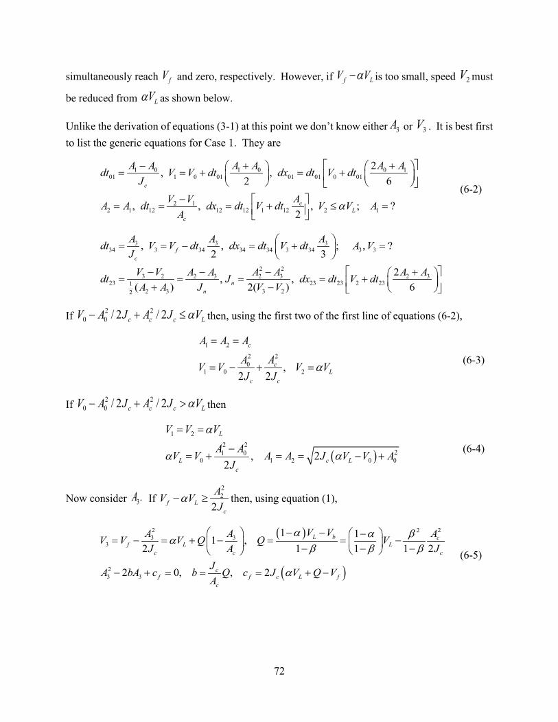
72

simultaneously reach fV and zero, respectively. However, if f LV Vα− is too small, speed 2V must

be reduced from LVα as shown below.

Unlike the derivation of equations (3-1) at this point we don’t know either 3A or 3V . It is best first to list the generic equations for Case 1. They are

1 0 1 0 0 101 1 0 01 01 01 0 01

2 12 1 12 12 12 1 12 2 1

2, ,2 6

, , , ; ?2

c

cL

c

A A A A A Adt V V dt dx dt V dtJ

AV VA A dt dx dt V dt V V AA

α

− + + = = + = + − = = = + ≤ =

(6-2)

3 3 334 3 34 34 34 3 34 3 3

2 23 2 2 3 2 3 2 3

23 23 23 2 2312 3 3 22

, , ; , ?2 3

2, ,( ) 2( ) 6

fc

nn

A A Adt V V dt dx dt V dt A VJ

V V A A A A A Adt J dx dt V dtA A J V V

= = − = + =

− − − + = = = = + + −

If 2 20 0 / 2 / 2c c c LV A J A J Vα− + ≤ then, using the first two of the first line of equations (6-2),

1 2

2 20

1 0 2,2 2

c

cL

c c

A A AA AV V V VJ J

α

= =

= − + = (6-3)

If 2 20 0 / 2 / 2c c c LV A J A J Vα− + > then

( )

1 22 2

21 00 1 2 0 0, 2

2

L

L c Lc

V V VA AV V A A J V V A

J

α

α α

= =

−= + = = − +

(6-4)

Now consider 3.A If 22

2f Lc

AV VJ

α− ≥ then, using equation (1),

( )

( )

2 223 3

3

23 3

1 11 ,2 1 1 1 2

2 0, , 2

L b cf L L

c c c

cf f c L f

c

V VA A AV V V Q Q VJ A J

JA bA c b Q c J V Q VA

α α βαβ β β

α

− − −= − = + − = = − − − −

− + = = = + −

(6-5)

73

min

22 3 3

3 33

2

33

, ,2

101 1 2

ff f L

c c c c

f c c cL

c c

VA AQ QA b b c V A V QJ A A J A

V J J AA Q VA A A

α

α ββ β

∂= ± − = − + + = −

∂

∂ −= → = = − ∂ − −

(6-6)

The quantity fV can, as shown in equations (6-6), be expressed as a parabolic function of 3A ,

which has a single minimum point at the value of min3A given in equations (6-6). If we assume, as

we do in the system that 1/ 2 and 0.25 , 0.25 /c cA g J g sα β= = = = then

min3

116LA V g= −

The maximum value of min3A is 0.25g.

min3A reaches this value if 5 3.07 m/s,16LV g= = which is

substantially lower than any practical line speed. Thus, of the two solutions for 3,A only the lower one has physical meaning. Thus

23 fA b b c= − − (6-7)

Can the quantity 2fb c− ever be negative? We see from equation (6-5) that

( )2 2 2cf c c f L

c c

J Qb c J Q J V VA A

α

− = − + −

The smallest value fV can have in Case 1 is .LVα Assuming this value, we see that the radical is certainly positive if

2 221 2 .

1 1 2c c

Lc c

A AQ VJ J

α ββ β

−= − ≥ − −

Using the values given after equation (6-6), we see that the radical is always positive if

9 5.52 m/s.16LV g> =

Since this value of line speed is less than practical values, the radical in equation (6-7) is always positive.

Now, if 22

2f Lc

AV VJ

α− < there are two cases:

74

If 2 20

0 2c

fc c

A AV VJ J

− + ≥

2

2 3 2 3,2

cc f

c

AA A A V V VJ

= = = = − (6-8)

If 2 20

0 2c

fc c

A AV VJ J

− + <

2 220 02

0 2 3 1 0

20

1 2 3 0

,2 2

12 2

f c fc c c

fc

A AAV V A A A J V VJ J J

AV V V V VJ

− + = = = = − +

= = = + −

(6-9)

Case 2

From point 0 to point 1 positive jerk cJ is applied up to an acceleration 1A that will be calculated using equation (6-1). Points 1 and 2 are at the same location. From point 2 to point 3 negative jerk nJ is applied until at point 3 maximum negative jerk cJ must be applied until at point 4 the

speed reaches fV just as the acceleration vanishes. The acceleration and speed at point 3 are calculated from equations (6-7) and (6-5) respectively. The equation set is as follows.

1 0 1 0 0 101 1 0 01 01 01 0 01

12 1 2

3 3 334 3 34 34 34 3 34 3 3

2 23 2 2 3 2 3 2 3

23 23 23 2 2312 3 3 22

2, ,2 6

0,

, , , , ?2 3

2, ,( ) 2( ) 6

c

fc

nn

A A A A A Adt V V dt dx dt V dtJ

dt A AA A Adt V V dt dx dt V dt A VJ

V V A A A A A Adt J dx dt V dtA A J V V

− + + = = + = +

= =

= = − = + =

− − − += = = = ++ −

(6-10)

To find the values of 1 1andA V note from the first row of equation set (6-10) that

2 2

1 01 0 .

2 c

A AV VJ−

= + (6-11)

By substituting equation (6-11) into equation (6-1) and letting 1A A= we get

2 20 1 1

0 12 2 L

c c c

A A AV V QJ J A

α

− + = + −

(6-12)

75

which can be written in the form

21 1 02 0pA bA c+ − = (6-13)

where b is given in the equation set (6-5) and ( )20 0 02 / 2p c L cc J V Q V A Jα= + − + . Equation (6-

10) has one positive solution:

21 0 pA b b c= − + + (6-14)

If 2 20

0 2c

fc c

A AV VJ J

− + ≥ then

1 2A A= from (6-14), 1 2V V= from (6-11); 3A from (6-7), 3V from (6-5).

If 2 20

0 2c

fc c

A AV VJ J

− + < then

2 20

0

2 20 0

1 2 3 0 1 2 3 0

2

1,2 2 2

cf

c c

c f fc c

A AV VJ J

A AA A A J V V V V V V VJ J

− + <

= = = − + = = = + −

Case 3

From point 0 to point 1 positive jerk cJ is applied to 1.A if 1 cA A= acceleration is constant from

point 1 to point 2, which is the same as point 3. Finally maximum negative jerk cJ− is applied

until the speed reaches fV while acceleration vanishes. The equation set is as follows:

1 0 1 0 0 101 1 0 01 01 01 0 01

3 3 334 3 34 34 34 3 34 2 3 3 2 1

23

2, ,2 6

, , , ,2 3

0

c

fc

A A A A A Adt V V dt dx dt V dtJ

A A Adt V V dt dx dt V dt V V A A AJ

dt

− + + = = + = +

= = − = + = = =

=

(6-15)

2 1 112 12 12 1 12

1

,2

V V Adt dx dt V dtA− = = +

If 2 20

0 2c

fc c

A AV VJ J

− + ≥ then

76

1 2 3

2 2 20

1 0 2 3,2 2 2

c

c cf

c c c

A A A AA A AV V V V VJ J J

= = =

= − + = = −

If 2 20

0 2c

fc c

A AV VJ J

− + < then

20

1 2 3 0

20

1 2 3 1 0

2

12 2

c fc

c

AA A A J V VJ

AV V V V VJ

= = = − +

= = = + −

Case 4

From point 0 to point 1 negative jerk cJ is applied until the negative acceleration at point 1 satisfies

equation (6-1). Then a small negative jerk nJ is applied between points 1 and 2 until the

acceleration reaches cA− at point 2, where the speed is .LVα Negative acceleration cA− is

continued from point 2 to point 3 and then positive jerk cJ is applied from point 3 to point 4, at

which speed reaches fV just as acceleration vanishes. The equation set is as follows:

1 0 1 0 0 1

01 1 0 01 01 01 0 01 1 1

2 22 1 2 1 2 1 1 2

12 12 12 1 12 211 2 1 22

3 3 334 3 34 34 34 3 34

2, , , , ?2 6

2, , ,( ) 2( ) 6

, ,2 3

c

n Ln

fc

A A A A A Adt V V dt dx dt V dt A VJ

V V A A A A A Adt J dx dt V dt V VA A J V V

A A Adt V V dt dx dt V dtJ

α

− + + = = + = + = − − − − + = = = = + = + − −

− = = − = +

3 2

3 2 223 23 23 2 23

2

,

,2

A A

V V Adt dx dt V dtA

=

− = = +

(6-16)

We need first to consider the portion of the curve below .LVα Then

If 2

2c

L fc

AV VJ

α − ≥

3

2

3 2

c

cf

c

A AAV VJ

=

= + (6-17)

77

If 2

2c

L fc

AV VJ

α − <

( )3

3

2 c L f

L

A J V V

V V

α

α

= −

=

(6-18)

In both of these cases 2 2 3and .LV V A Aα= =

To compute 1 1andA V we need to consider two cases.

Case 1: 2 20

0 .2 2

cL

c c

A AV VJ J

α+ − >

In this case, set 1V from the first row of equation set (6-16) equal to V in equation (6-1). Thus

2 2

10 11 0 1

2 Lc c

AA AV V V QJ A

α −

= + = + −

(6-19)

which gives the following quadratic equation for 1.A

21 1 02 0mA b A c− + = (6-20)

in which b is found from equation set (6-5) and

20

0 022m c L

c

Ac J V Q VJ

α

= + − −

. (6-211)

Thus

21 0

2 20 1

1 0 2 2

m

c c

A b b c

A AV VJ J

= − + −

= + − (6-21)

which takes into account that 1 0.A <

Case 2: 2 20

0 .2 2

cL

c c

A AV VJ J

α+ − ≤

Now there are two subcases:

78

Case 2.1: 2 20

0 2c

fc c

A AV VJ J

+ − ≥

1 2 3

2 20

1 2 0 2 2

c

c

c c

A A A AA AV V VJ J

= = =

= = + − (6-23)

Case 2.2: 2 20

0 2c

fc c

A AV VJ J

+ − <

20

1 2 3 0

20

1 2 3 0

2

12 2

c fc

fc

AA A A J V VJ

AV V V V VJ

= = = − + −

= = = + +

(6-24)

Case 5

Negative jerk is applied from point 0 to point 1, at which point 1 1andA V are determined exactly as

in Case 4. Negative jerk nJ is then applied from point 1 to point 2 (points 2 and 3 are coincident)

until at point 3 maximum positive jerk cJ is applied until the speed reaches fV just as acceleration vanishes. The determining equation set is as follows:

1 0 1 0 0 101 1 0 01 01 01 0 01 1 1

2 22 1 2 1 2 1 1 2

12 12 12 1 1212 1 1 22

23 2 3

3 334 3 34

2, , ; , ?2 6

2, ,( ) 2( ) 6

0,

, ,2

c

nn

fc

A A A A A Adt V V dt dx dt V dt A VJ

V V A A A A A Adt J dx dt V dtA A J V V

dt A AA Adt V V dt

J

− + + = = + = + = − − − − + = = = = + + − −

= =

−= = − 3

34 34 3 34 3 3; , ?3Adx dt V dt A V = + =

(6-25)

To determine 3 3,A V note that

( )

23 23

3 3 3

2 23 3 3

1 2 2 02 /

2 0

f L c L fc c c c

f f

AA QV V V Q A A J V Q VJ A A J

A b A c A b b c

α α

= + = + − → + − + − =

+ − = → = − +

(6-26)

79

Case 6

Maximum negative jerk cJ is applied from point 0 to point 1, where 1 cA A= − . Points 1 and 2 are

coincident. Maximum negative acceleration cA− is applied from point 2 to point 3 and at point 3

maximum positive jerk cJ is applied until the speed reaches fV just as acceleration vanishes. The governing equation set is as follows:

1 0 1 0 0 101 1 0 01 01 01 0 01

12 1 2 3 2 1

3 3 334 3 34 34 34 3 34

2 3 223 23 23 2 23

2

2, ,2 6

0, ,

, ,2 3

,2

c

fc

A A A A A Adt V V dt dx dt V dtJ

dt A A A V VA A Adt V V dt dx dt V dt

JV V Adt dx dt V dt

A

− + + = = + = + − = = = =

− = = − = +

− = = + −

(6-27)

7. Headway Needed to Delay Speed Reduction

Consider a vehicle 0 that is commanded to reduce speed from a line speed 1LV to a speed

2LV at

time 0.t = The slow-down transition takes an amount of time mT and occurs over a distance

.mD Assume vehicle 1 is a distance 1dP behind vehicle 0 and traveling at speed 1LV is close

enough that it must be commanded to slow down to speed 2LV as close to immediately as possible.

Taking into account a computational interval t∆ vehicle 1 may not start slowing down until a time t∆ later. Thus, once it has reached speed

2LV its distance-time curve is given by the equation

( )1 21 1 L m L mx dP V t D V t t T= − + ∆ + + −∆ − (7.1)

We need to know how far behind vehicle 0 vehicle 2 must be so that it can delay slowing down until it reaches the speed-change command point, i.e., the point along the guideway at which vehicle 0 started to slow down. Assume this is the case. Then vehicle 2 doesn’t reach speed

2LVuntil it reaches the position ahead of the position vehicle 0 began to slow down by an amount

1.L mV t D∆ + Once vehicle 2 has reached speed

2LV its distance-time curve is given by the equation

80

Figure 6. The Kinematics of a Speed Reduction.

1 2

1

22 L m L m

L

dPx V t D V t t TV

= ∆ + + − −∆ −

(7.2)

Substituting the time 1

2m

L

dPt t TV

= + ∆ + into equation (1.1) we see that the separation between

vehicle 1 and vehicle 2 at this time is

( )

1 2 1

1

2

2

1

21 2 1

1 2

L m L L mL

LL h

L

dPx x dP V t D V V t DV

VdP dP V T t

V

− = − + ∆ + + − ∆ −

= − + ≥ + ∆

(7.3)

Thus, the desired result is

(7.4)

( ) 1

1

2

2 1L

L hL

VdP V T t dP

V≥ + ∆ +

81

8. Emergency Stop

An emergency stop starts with arbitrary initial acceleration 0A and initial speed 0V . The vehicle

is subjected to a maximum negative jerk maxJ up to a point 1 at which the deceleration is the

emergency value eA− and then decelerates at that maximum rate until a point 2, where positive

jerk maxJ is applied until the vehicle stops at a point 3. Using the basic transition equations (1-2), the emergency-stop transition is set up with the following equations:

( )( )

( ) ( )

01 0 max 1 0 01 0 01 01 0 01 0

23 max 2 23 23 23 2 23

12 1 2 12 12 1 12

1 01 2 1 12 3 2 23

1 01 2 1 12 3 2

( ) / , ( ) / 2, 2 / 6

/ , / 2, / 3

/ , / 2, ,, ,

e e e

e e e

e e

dt A A J V V dt A A dx dt V dt A A

dt A J V dt A dx dt V dt A

dt V V A dx dt V dt At dt t t dt t t dtx dx x x dx x x d

= + = − − = + − = = = −

= − = −

= = + = += = + = + 23x

The transition is then run using the following code:

0

1

max

0 0 0

2

1 1 1

3

max

2 2 2

JerkState ( t, Jerk, A , V , x , A, V, x)

0State ( t, Jerk, A , V , x , A, V, x)

State ( t, Jerk, A , V , x , A, V, x)

0

t t tif t t then

J

elseif t t thenJerk

elseif t t thenJerk J

elseJerk

end if

∆ = −<

= −∆<=∆<= +∆

=

9. Distance to Reach Station Speed

When a vehicle is ready to leave a station it may be advancing in the station at any speed 0V below

station speed sV and at any acceleration 0A within the comfort range. It must not be permitted to

accelerate to line speed if at that moment it would exceed sV its nose would not have reached the

downstream end of the station. The criterion to leave is thus that the distance to reach sV is greater than the distance to the downstream end of the station. Using the notation of Section 3, let the

82

distance from initiation of the acceleration transition to the speed sV be 0 .sdx Then, following the notation of Section 3, we must consider two cases:

2sV V≤

( )0 01 1 / .s s cdx dx V V A= + −

2sV V>

( )0 01 12 2 2 2 2 / 6s s s c sdx dx dx dt V dt A A= + + + +

in which

( )

( )

2

2 22 2 2 2 2 2

22 2

0 01 12 2 2 2 2

or 02 2

1or 2

3 / 6

s c n s

n ns c s s s c s s

s c c n sn

s s s c n s

A A J dtJ JV V A dt dt dt A dt V V

dt A A J V VJ

dx dx dx dt V dt A J dt

= −

= + − − + − =

= − − −

= + + + −

in which the minus sign before the square root is taken because we know that when

2 2, 0.s sV V dt→ →

10. The Distance to Slip a Given Amount

Assume a series of slip transitions which begin and end at line speed. Assume that the minimum speed in the transition, mV is low enough so that the cruising time at mV is zero. Then if LV is the

line speed, if 21 1/ then else .m c c c L cV A J A J V A A< = = The transition time is

1

1

2 L mm

c

V V AT

A J −

= +

.

The slip S is

( ) / 2L m mS V V T= −

and the distance traveled to slip S is

Distance = .L mV T S−

These quantities are calculated and plotted in the following table for 16LV = m/s.

83

Table 1

Distance Traveled During Slip Transition

g = 9.807 m/s^2

Ac = 2.452 m/s^2

Jc = 2.452 m/s^3

VL = 16 m/s

Vmin A1 Tm Slip Dist

m/s m/s^2 sec m m

16.0 0.00 0.00 0.00 0.00

15.8 0.70 1.14 0.11 18.17

15.6 0.99 1.62 0.32 25.53

15.4 1.21 1.98 0.59 31.07

15.2 1.40 2.28 0.91 35.65

15.0 1.57 2.55 1.28 39.60

14.8 1.72 2.80 1.68 43.10

14.6 1.85 3.02 2.12 425

14.4 1.98 3.23 2.59 49.12

14.2 2.10 3.43 3.08 51.75

14.0 2.21 3.61 3.61 54.19

13.8 2.32 3.79 4.17 546

13.6 2.43 3.96 4.75 58.57

13.4 2.45 4.12 5.36 60.58

13.2 2.45 4.28 6.00 62.55

13.0 2.45 4.45 67 64.49

12.8 2.45 4.61 7.38 639

12.6 2.45 4.77 8.12 68.26

12.4 2.45 4.94 8.89 70.10

12.2 2.45 5.10 9.69 71.91

84

12.0 2.45 5.26 10.53 73.68

11.8 2.45 5.43 11.40 75.42

11.6 2.45 5.59 12.30 77.13

11.4 2.45 5.75 13.23 78.81

11.2 2.45 5.92 14.20 80.45

11.0 2.45 6.08 15.20 82.06

10.8 2.45 24 123 83.64

10.6 2.45 41 17.29 85.19

10.4 2.45 57 18.39 86.70

10.2 2.45 6.73 19.52 88.18

10.0 2.45 6.89 20.68 89.63

85

Potential Headway Violation upon Decelerating into a Station

Figure 1. The velocity profiles of a pair of vehicles entering a station.

Consider a vehicle #1 decelerating into a station to station speed staV , followed by a vehicle #2 a time Line Headway behind undergoing the same maneuver. Let the position of vehicle #1 at time zero be (0) 0.x = The times, accelerations, speeds, and positions of vehicle #1 at the points 1, 2, 3 in Figure 110 are as follows:

01 1 01 01 01 01

23 2 23 23 23 2 23

1 212 12 12 1 12

1 01 2 1 12 3 2 23

1 01 2 1 12 3 2 23

, ,2 6

, ,2 3

,2

, ,, ,

c c cL L

c

c c csta

c

c

c

A A Adt V V dt dx dt V dtJA A Adt V V dt dx dt V dtJ

AV Vdt dx dt V dtA

t dt t t dt t t dtx dx x x dx x x dx

= = − = −

= = + = −

− = = −

= = + = += = + = +

(1)

From equations (1) we find

2 2

03 01 23 1212

2 2c c c L sta c

L stac c c c c c

A A A V V Adt dt dt dt V VJ A J J A J

−= + + = + − − − = +

(2)

10 For the methodology, see the internal paper “Speed and Position vs. Time”

2

V

t

0 1 3

Line Headway

VL

1

2

Vstation

86

Thus, the maneuver time from line speed to station speed is

L sta cm

c c

V V ATA J−

= + (3)

From equations (1) we also find

( )

( ) ( )( ) ( ) ( )

( ) ( )

2 2 21 2

03 01 23 12 1 2

2

1 2 1 2

03

2 6 3 2

1 12 2

2 2

c c c cL sta

c c c c c

c c cL sta L sta L sta L sta

c c c c c

L sta L staL sta c

c c

A A A A V Vdx dx dx dx V V V VJ J J J A

A A AV V V V V V V V V V V VJ A J A J

V V V VV V A dtA J

−= + + = + + − − + +

= + + − + = + + − − +

+ + −= + =

(4)

Thus, the distance traveled from line speed to station speed is

( )2

L stam m

V VD T

+= (5)

Using the above canonical formulation, the acceleration, speed, and position of vehicle 1 at any value of t are as follows:

( )

1

1 2 1 1 1 1

2 3 2 2 2 2

0 : , , ,2 6

: , , ,2

: , , ,2 3

c L L

c

cc c

A At t t t A J t V V t x t V t

At t t t t t A A V V tA x x t V t

A A At t t t t t A A J t V V t x x t V t

≤ ≤ ∆ = = − ∆ = + ∆ = ∆ + ∆

≤ ≤ ∆ = − = − = + ∆ = + ∆ + ∆

− + ≤ ≤ ∆ = − = − + ∆ = + ∆ = + ∆ + ∆

(6)

For vehicle #2 up to time t LineHeadway= the speed stays constant at LV and the distance traveled is

Lx V t= . For t LineHeadway> we can obtain the acceleration, speed, and position as functions of time by making the following substitutions in equations (5): t t LineHeadway→ −

87

( )

1

1 2 1 1 1 1

0 : 0, ,

: , , ,2 6

: , , ,2

h

h L L h

h h h c L L

h h c

T LineHeadwayt T A V V x V t T

A AT t t T t t T A J t V V t x t V t

AT t t T t t t t A A V V tA x x t V t

=

≤ ≤ = = = −

≤ ≤ + ∆ = − = − ∆ = + ∆ = ∆ + ∆

+ ≤ ≤ + ∆ = − = − = + ∆ = + ∆ + ∆

( )2 3 2 2 2 2: , , ,

2 3c

h h c c

A A AT t t T t t t t A A J t V V t x x t V t− + + ≤ ≤ + ∆ = − = − + ∆ = + ∆ = + ∆ + ∆

(7)

The Minimum Headway

Figure 2. A pair of vehicles moving to the right.

Assume vehicle #1 stops due to a failure at deceleration fA and jerk .fJ From equation (5), the stopping distance of vehicle #1 is

1 11 2

f

f f

AV VDA J

= +

(8)

After a control time delay ,ct vehicle #2 stops at the emergency deceleration rate eA and

emergency jerk .eJ Its stopping distance is therefore

2 22 2 2

ec

e e

AV VD V tA J

= + +

(9)

Assuming the length of each of the two vehicles is L , the minimum allowable separation between them is

min 2 1H L D D= + − (10)

#1 #2

D1

L D2

Hmin

V1 V2

88

The minimum permissible time headway is therefore

min

2

HMinHeadwayV

=

(11)

A program to calculate the acceleration, speed, positions profiles and the minimum headway is given in the Appendix. Some results are given in Figures 3 and 4.

Figure 3. Kinematics of motion of a pair of vehicles decelerating to station speed.

Figure 4. Separation and minimum allowable separation between two vehicles entering a station.

0 1 2 3 4

TIME, seconds

-10

0

10

20

30

40

Acce

lerati

on, s

peed

, and

dista

nce t

rave

lled i

n MKS

units Acceleration of veh 1

Speed of veh 1Distance veh 1 has traveledAcceleration of veh 2Speed of veh 2Distance veh2 has traveled

0 1 2 3 4

TIME, seconds

0

1

2

3

4

5

6

7

8

9

10

11

12

13

Actua

l and

mini

mum

sepa

ratio

ns, m

eters

Separation between veh 1 and 2Minimum allowable separation

89

The parameters used in Figures 3 and 4 are those given at the beginning of the program shown in the Appendix. Many runs can be made for different accelerations and jerks. For the set shown in the program, runs were made with different line headways and control time constants to obtain the maximum negative separations as shown in Table 1 and as calculated by the program.

Table 1. Maximum headway violations for the cases shown.

\ct LineHeadway → 0.5 1.0 1.3 1.5

0.05 -3.25 -1.03 0 0 0.10 -3.80 -1.59 -0.03 0 0.15 -4.36 -2.15 -0.60 0 0.20 -4.92 -2.71 -1.17 -0.01

It is seen that if the line headway between two vehicles sequentially entering a station is to be as low as one second, the control time constant must be quite small, but not particularly small using contemporary technology. Note from Figure 4 that in the case shown the small headway violation increases from zero back to zero in about one second.

In this work, we considered only the portion of the maneuver from line speed to station speed. Further development of the program included in the Appendix shows that, since the second of the pair of vehicles will be stopping at least one berth behind the first, there is no headway violation in the maneuvers from station speed to rest.

Appendix 'This program MINHEAD.BAS calculates the minimum headway permissible 'between a pair of vehicles decelerating into a station 'Units are MKS DEFDBL A-Z DIM Counter AS INTEGER DIM A(1 TO 2) AS DOUBLE 'acceleration of vehicles 1 & 2 DIM V(1 TO 2) AS DOUBLE 'speed of vehicles 1 & 2 DIM X(1 TO 2) AS DOUBLE 'position of vehicles 1 & 2 DIM t4(1 TO 2) AS DOUBLE 'time at end of station-speed section DIM t5(1 TO 2) AS DOUBLE 'time at command to constant deceleration DIM t6(1 TO 2) AS DOUBLE 'time at command to constant jerk DIM t7(1 TO 2) AS DOUBLE 'time at maneuver end, total maneuver time DIM X1(1 TO 2) AS DOUBLE 'position of command to constant deceleration DIM X2(1 TO 2) AS DOUBLE 'position of command to constant jerk DIM X3(1 TO 2) AS DOUBLE 'position at beginning of station-speed section DIM X4(1 TO 2) AS DOUBLE 'position at end of station-speed section DIM X5(1 TO 2) AS DOUBLE 'position of command to constant deceleration DIM X6(1 TO 2) AS DOUBLE 'position of command to constant jerk DIM X7(1 TO 2) AS DOUBLE 'position at maneuver end,total maneuver distance DIM D(1 TO 2) AS DOUBLE 'stopping distances of vehicles 1 & 2

90

g = 9.80665 'acceleration of gravity Ac = .25 * g 'comfort deceleration Jc = .25 * g 'comfort jerk tJ = Ac / Jc 'jerk time constant Af = .4 * g 'maximum failure deceleration Jf = .4 * g 'maximum failure jerk Ae = .4 * g 'emergency deceleration Je = .8 * g 'emergency jerk VL = 12 'line speed Vsta = 8 'station speed tc = .15 'time constant Lveh = 2.743 'vehicle length B = 3.048 'berth length LineHeadway = .5 'time headway between vehicles while at line speed t = 0 'start time dt = .01 'computational time interval 'Calculation of the maneuver increments and transition speeds dt01 = tJ V1 = VL - dt01 * Ac / 2 dx01 = dt01 * (VL - Ac * dt01 / 6) dt23 = tJ V2 = Vsta + dt23 * Ac / 2 dx23 = dt23 * (V2 - dt23 * Ac / 3) dt12 = (V1 - V2) / Ac dx12 = dt12 * (V1 - dt12 * Ac / 2) dx34 = 10 'distance vehicle 1 travels at station speed dt34 = dx34 / Vsta 'time of veh 1 at station speed dt45 = tJ V5 = Vsta - dt45 * Ac / 2 dx45 = dt45 * (Vsta - dt45 * Ac / 6) dt67 = tJ V6 = dt67 * Ac / 2 dx67 = dt67 * (V6 - dt67 * Ac / 3) dt56 = (V5 - V6) / Ac dx56 = dt56 * (V5 - dt56 * Ac / 2) 'Times and position increments at the transition points t1 = dt01 t2 = t1 + dt12 t3 = t2 + dt23 t4(1) = t3 + dt34 'this and following times for veh 1 t5(1) = t4(1) + dt45 t6(1) = t5(1) + dt56 t7(1) = t6(1) + dt67 'maneuver time t4(2) = t3 + dt34 - B / Vsta 'this and following times for veh 2 t5(2) = t4(2) + dt45 t6(2) = t5(2) + dt56 t7(2) = t6(2) + dt67 'maneuver time X1(1) = dx01 X2(1) = X1(1) + dx12 X3(1) = X2(1) + dx23 X4(1) = X3(1) + dx34 X5(1) = X4(1) + dx45 X6(1) = X5(1) + dx56

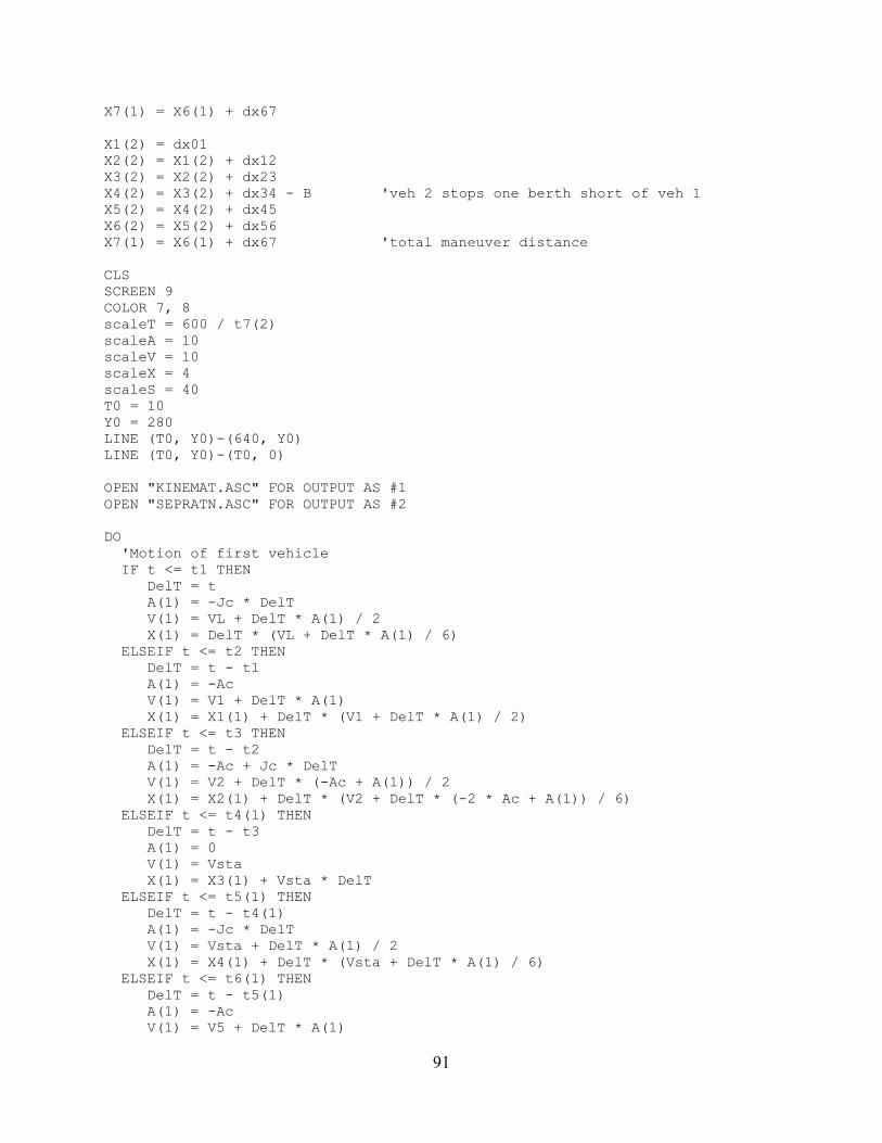
91

X7(1) = X6(1) + dx67 X1(2) = dx01 X2(2) = X1(2) + dx12 X3(2) = X2(2) + dx23 X4(2) = X3(2) + dx34 - B 'veh 2 stops one berth short of veh 1 X5(2) = X4(2) + dx45 X6(2) = X5(2) + dx56 X7(1) = X6(1) + dx67 'total maneuver distance CLS SCREEN 9 COLOR 7, 8 scaleT = 600 / t7(2) scaleA = 10 scaleV = 10 scaleX = 4 scaleS = 40 T0 = 10 Y0 = 280 LINE (T0, Y0)-(640, Y0) LINE (T0, Y0)-(T0, 0) OPEN "KINEMAT.ASC" FOR OUTPUT AS #1 OPEN "SEPRATN.ASC" FOR OUTPUT AS #2 DO 'Motion of first vehicle IF t <= t1 THEN DelT = t A(1) = -Jc * DelT V(1) = VL + DelT * A(1) / 2 X(1) = DelT * (VL + DelT * A(1) / 6) ELSEIF t <= t2 THEN DelT = t - t1 A(1) = -Ac V(1) = V1 + DelT * A(1) X(1) = X1(1) + DelT * (V1 + DelT * A(1) / 2) ELSEIF t <= t3 THEN DelT = t - t2 A(1) = -Ac + Jc * DelT V(1) = V2 + DelT * (-Ac + A(1)) / 2 X(1) = X2(1) + DelT * (V2 + DelT * (-2 * Ac + A(1)) / 6) ELSEIF t <= t4(1) THEN DelT = t - t3 A(1) = 0 V(1) = Vsta X(1) = X3(1) + Vsta * DelT ELSEIF t <= t5(1) THEN DelT = t - t4(1) A(1) = -Jc * DelT V(1) = Vsta + DelT * A(1) / 2 X(1) = X4(1) + DelT * (Vsta + DelT * A(1) / 6) ELSEIF t <= t6(1) THEN DelT = t - t5(1) A(1) = -Ac V(1) = V5 + DelT * A(1)

92

X(1) = X5(1) + DelT * (V5 + DelT * A(1) / 2) ELSEIF t < t7(1) THEN DelT = t - t6(1) A(1) = -Ac + Jc * DelT V(1) = V6 + DelT * (-Ac + A(1)) / 2 X(1) = X6(1) + DelT * (V6 + DelT * (-2 * Ac + A(1)) / 6) ELSE A(1) = 0 V(1) = 0 X(1) = X7(1) END IF 'Motion of second vehicle tsec = t - LineHeadway IF tsec <= 0 THEN DelT = tsec A(2) = 0 V(2) = VL X(2) = DelT * VL ELSEIF tsec <= t1 THEN DelT = tsec A(2) = -Jc * DelT V(2) = VL + DelT * A(2) / 2 X(2) = DelT * (VL + DelT * A(2) / 6) ELSEIF tsec <= t2 THEN DelT = tsec - t1 A(2) = -Ac V(2) = V1 + DelT * A(2) X(2) = X1(2) + DelT * (V1 + DelT * A(2) / 2) ELSEIF tsec <= t3 THEN DelT = tsec - t2 A(2) = -Ac + DelT * Jc V(2) = V2 + DelT * (-Ac + A(2)) / 2 X(2) = X2(2) + DelT * (V2 + DelT * (-2 * Ac + A(2)) / 6) ELSEIF tsec <= t4(2) THEN DelT = tsec - t3 A(2) = 0 V(2) = Vsta X(2) = X3(2) + Vsta * DelT ELSEIF tsec <= t5(2) THEN DelT = tsec - t4(2) A(2) = -Jc * DelT V(2) = Vsta + DelT * A(2) / 2 X(2) = X4(2) + DelT * (Vsta + DelT * A(2) / 6) ELSEIF tsec <= t6(2) THEN DelT = tsec - t5(2) A(2) = -Ac V(2) = V5 + DelT * A(2) X(2) = X5(2) + DelT * (V5 + DelT * A(2) / 2) ELSEIF tsec < t7(2) THEN DelT = tsec - t6(2) A(2) = -Ac + Jc * DelT V(2) = V6 + DelT * (-Ac + A(1)) / 2 X(2) = X6(2) + DelT * (V6 + DelT * (-2 * Ac + A(1)) / 6) ELSE A(2) = 0 V(2) = 0

93

X(2) = X7(2) END IF D(1) = .5 * V(1) * (V(1) / Af + Af / Jf) 'stopping distance of veh #1 D(2) = .5 * V(2) * (V(2) / Ae + Ae / Je) 'stopping distance of veh #2 Separation = X(1) - X(2) IF Separation < Lveh + V(2) * tc THEN SLEEP IF V(2) > 0 THEN Headway = Separation / V(2) MinSeparation = Lveh + V(2) * tc + D(2) - D(1) IF V(2) > 0 THEN MinHeadway = MinSeparation / V(2) dSep = Separation - MinSeparation IF dSep < MaxNegSep THEN MaxNegSep = dSep PSET (T0 + scaleT * t, Y0 - scaleA * A(1)), 14 PSET (T0 + scaleT * t, Y0 - scaleV * V(1)), 13 PSET (T0 + scaleT * t, Y0 - scaleX * X(1)), 12 PSET (T0 + scaleT * t, Y0 - scaleA * A(2)), 11 PSET (T0 + scaleT * t, Y0 - scaleV * V(2)), 10 PSET (T0 + scaleT * t, Y0 - scaleX * X(2)), 9 PSET (T0 + scaleT * t, Y0 - scaleS * Separation), 5 PSET (T0 + scaleT * t, Y0 - scaleS * MinSeparation), 6 'PRINT USING "#####.##"; t; A(1); V(1); X(1) ; A(2); V(2); X(2); Separation; MinSeparation 'PRINT USING "#####.##"; t; V(2); Separation; Separation - Lveh - V(2) * tc; MinSeparation; dSep; Headway; MinHeadway IF Counter = 20 THEN Counter = 0 'SLEEP END IF Counter = Counter + 1 'WRITE #1, t, A(1), V(1), X(1), A(2), V(2), X(2) 'WRITE #2, t, Separation, MinSeparation t = t + dt LOOP UNTIL t > t7(2) + 1 PRINT " MaxNegSep = "; PRINT USING "###.##"; MaxNegSep CLOSE #1 CLOSE #2

94

Headway Needed to Delay Speed Reduction

Figure 1. The Kinematics of a Speed Reduction.

Consider a vehicle 0 that is commanded to reduce speed from a line speed 1LV to a speed

2LV at

time 0.t = The slow-down maneuver takes an amount of time mT and occurs over a distance

.mD Assume vehicle 1 is a distance 1dP behind vehicle 0 and traveling at speed 1LV . Assume

that it is close enough to vehicle 0 that it must be commanded to slow down to speed 2LV as close

to immediately as possible. Taking into account a computational interval t∆ vehicle 1 may not start slowing down until a time t∆ later. Thus, once it has reached speed

2LV its distance-time curve is given by the equation

95

( )1 21 1 L m L mx dP V t D V t t T= − + ∆ + + −∆ − (1)

We need to know how far behind vehicle 0 vehicle 2 must be so that it can delay slowing down until it reaches the speed-change command point, i.e., the point along the guideway at which vehicle 0 started to slow down. Assume this is the case. Then vehicle 2 doesn’t reach speed

2LVuntil it reaches the position ahead of the position vehicle 0 began to slow down by an amount

1.L mV t D∆ + Once vehicle 2 has reached speed

2LV its distance-time curve is given by the equation

1 2

1

22 L m L m

L

dPx V t D V t t TV

= ∆ + + − −∆ −

(2)

Substituting the time 1

2m

L

dPt t TV

= + ∆ + into equation (1) we see that the separation between

vehicle 1 and vehicle 2 at this time is

( )

1 2 1

1

2

2

1

21 2 1

1 2

L m L L mL

LL h

L

dPx x dP V t D V V t DV

VdP dP V T t

V

− = − + ∆ + + − ∆ −

= − + ≥ + ∆

(3)

in which Th is the minimum permissible time headway. Thus, the desired result is

( ) 1

1

2

2 1L

L hL

VdP V T t dP

V≥ + ∆ +

96

On-Line Deceleration

Figure 1. Speed profile of vehicle decelerating.

1. Introduction

To reduce the required length of off-line guideway in a PRT system, it is possible to initiate deceleration before a vehicle is clear of mainline traffic. The question that this memo answers is this: What is the relationship between the distance traveled by a decelerating vehicle while still on-line and the reduction in on-line headway? This memo shows that by sacrificing a small amount of on-line headway, the length of the by-pass guideway can be reduced substantially.

2. Deceleration at constant negative jerk.

Figure 1 is a plot of speed V vs. time t and illustrates the speed profile of a vehicle decelerating from a line speed LV into a station. At first negative jerk cJ is applied until at a

point 1, the deceleration reaches the comfort value .cA The vehicle then decelerates at the

comfort value until it either stops or assumes the station speed. For the time interval 10 t t≤ ≤ the equations of motion are

2 3

, ,2 6c L c L ct tx J t x V J x V t J= − = − = −&& & (1)

At time 1t 1 1c

c cc

Ax A J t tJ

= − = − ∴ =&& (2)

Then

97

2 2

1

2

01

12 2

6

c cL c L

c c

c cL

c c

A AV V J VJ J

A Ax VJ J

= − = −

= −

(3)

The distance the vehicle moves backwards relative to or closes up to a vehicle behind it traveling at constant speed LV is called the slip distance, which if the vehicle slows down a time t1 is

3

01 1 01 26c

Lc

AS V t xJ

= − = (4)

3. Headway sacrificed during constant-jerk motion

Headway ht is defined as the time interval between the passage of the nose of one vehicle and the passage of the next relative to a stationary point. The distance traveled by a vehicle moving at speed VL during this time interval is L hV t . Thus, the headway lost to point 1 if a vehicle begins to decelerate while still on the main line is

3

012 .

6c

hL c L

S AtV J V

∆ = = (5)

For times less than 1t substitute cJ t for cA from equations (1). Then we have

1/3

3 6,6

c L hL h

c

J V tt V t tJ

∆= ∆ =

(6)

Substituting t into the third of equations (1), we see that for 1t t< the distance traveled while

losing a headway of ht∆ is

1/3

6 L hL h

c

V tx V tJ

∆ = − ∆

(7)

For longitudinal motion the comfort values are 0.25 , 0.25 /c cA g J g s= = . Therefore,

assuming g = 9.80665 m/s2 we have from equation (5) 0.4086 /h Lt V∆ = . Assuming a minimum

speed of say 10 m/s, we find that up to point 1 0.041ht∆ = sec.

98

4. Headway sacrificed during constant-deceleration phase

Assuming that we can permit a greater loss of headway as a result of on-line deceleration, let the vehicle proceed to a point 2 at constant deceleration cA− where 2 12 2 1, and .t t t t t= ∆ = − The

constant deceleration region pertains until 22 / 2 .c cV A J≤ The speed and distance traveled during

this interval in which 21 2 / 2c cV V A J> > are

2 1 12

2212

12 1 12 12 122 2 2

c

c cc L

c

V V A t

A Atx V t A t V tJ

= − ∆

∆= ∆ − = ∆ − − ∆

(8)

The slip distance in traveling from point 1 to point 2 is

12 12 12 12 122c c

Lc

A AS V t x t tJ

= ∆ − = + ∆ ∆

(9)

Thus the total slip distance up to point 2 is

02

2

02 01 12 12 1222 3c c c

L hc c

A A AS S S t t V tJ J

= + = + + ∆ ∆ = ∆

(10)

where 02ht∆ is the headway lost in slowing down to point 2. Equation (10) can be rearranged into

the form

02

2212 12 2

22 0

2 3L hc c

c c c

V tA At tJ A J

∆ ∆ + ∆ − − =

(11)

the positive root of which is

02 02

2 22

12 2

2 8 1 12 2 3 2 3

L h L hc c c c c

c c c c c c c

V t V tA A A A JtJ J A J J A A

∆ ∆ ∆ = − + + − = − − (12)

5. Total headway sacrificed

The distance traveled in the time period 02t∆ is

2 2

02 01 12 12 126 2 2c c c c

L Lc c c

A A A Ax x x V t V tJ J J

= + = − + ∆ − − ∆

(13)

Substitute for 212t∆ from equation (11). Then equation (13) becomes

99

02

02

2 22

02 12 12

2 2 2

12 12 2

12

6 2 2

26 2 2 3

c c c cL L

c c c

c c c c c cLL L h

c c c c c c

cL h

c

A A A Ax V t V tJ J J

A A A A A AVV t V t tJ J J J A J

AV t tJ

= − + ∆ − − ∆

= − + ∆ − + ∆ − ∆ +

= + ∆ −∆

(14)

Substituting for 12t∆ from equation (12) we get

02 02 02

2 3

02 3 28 11 if

2 3 6c L c c

L h h hc c c L

A V J Ax V t t tJ A J V

= + ∆ − − ∆ ∆ ≥

(15)

If 02

3

26c

hc L

AtJ V

∆ < the distance traveled while losing a headway of 02h ht t∆ = ∆ is given by equation

(7). The reader can verify that at 02

3

26c

hc L

AtJ V

∆ = both equations (7) and (15) give the same result.

6. Range of Validity of equation (15)

As mentioned in Section 4, equation (15) is valid if 22 / 2 .c cV A J> From equations (3) and (8)

this condition becomes

2 2

2 12 12or t2 2

c c cLL c

c c c c

A A AVV V A tJ J A J

= − − ∆ > ∆ < − (16)

Substituting for 12t∆ from equation (12) and reducing, we get

02

02

02

02

2

2

2 2 2

2 2

2

2

8 12 3 2

8 1 2 13

8 1 4 4 13

12 3

L hc c L c

c c c c c

L h c L c

c c c c

L h c L c L c

c c c c c c

L c c ch

c c c L

V tA J V AJ A A A J

V t J V JA A A A

V t J V J V JA A A A A A

V A A AtA J J V

∆ − < −

∆ − < −

∆ − < − +

∆ < − +

(17)

100

Using the above values we find for 10LV = 02

1.6 sec, and for 20h Lt V∆ = = meters per second

023.6 sec.ht∆ = These values are much longer than would be of interest for this problem,

therefore equation (12) gives correct values for 12.t∆

7. The maximum on-line distance traveled.

We can now plot a curve of distance traveled while losing a headway of ht∆ . Note, from

equation (7) that at 0ht∆ = the rate of change of x with ht∆ is infinite. The form of equation

(15) shows that as a function of ht∆ x increases to a maximum and then at a certain point falls to zero and below. The maximum value of distance traveled can be found by setting to zero the derivate of 02x with respect to ht∆ . The result is

02

2

2

2 2

22

22

h

82 13

8 2 1or3

1 1 1or t2 3 2

L hL c c

c c c

L h c L c

c c c

cL

c c L

V tV J JA A A

V t J V JA A A

AVA J V

∆ = −

∆= +

∆ = +

(18)

To obtain the maximum on-line deceleration distance, substitute equation (18) into equation (15). This is not done here because ht∆ at the maximum distance is much too large to be of interest in short-headway PRT systems.

8. Solving equation (15) for 02ht∆

In the numerical solution for the transition, we calculate 02x and need to calculate the

corresponding value of 02

.ht∆ To do so, rewrite equation (15) in the form

101

02

02 02

02 02

202

23

2 2 2202 02

22 3

22 02 02 02

2

8 12 2 3

8 122 2 4 3

2 02 3

The rad

c c L ch h

L c c c

c c c L ch h h

L c L c c c

L c c ch h

c c L L L c c

x A A V Jt tV J J A

x A x A A V Jt t tV J V J J A

V A x x x A At tA J V V V J J

− + ∆ = ∆ −

− + − ∆ + ∆ = ∆ −

∆ − + − ∆ + − + =

2 202 02 02

2

2 2 202 02

2 2

ical is

2 3

2 22 3 12

L c c c

c c L L L c c

L c L c L L c c

c c c L c c c c L c

V A x x x A AA J V V V J J

V A V x A V V A x AA J A V J A A J V J

+ − − − − =

+ − − = + − −

(19)

Therefore

02

202 02

2

2

02 02 2

3

02 02 2

22 12

1 22 2 12

1 222 24

c c cL L Lh

c c L c c c L c

c c c cL L LL

L c c c c c c c

c cstop L stop

L c c c

A x A x AV V VtA J V A A J V J

A A A AV V VV x xV A J J A A J J

A AD x V D xV J A J

∆ = + − − + − −

= + − − − + − −

= − − − − −

(20)

in which stopD is the stopping distance from speed .LV Since stopD must be substantially longer

than 02 ,x the term under the square-root sign is always positive in practical cases. The minus

sign before the radical is the correct one because equation (20) then reduces to equation (5) if 01x

is substituted for 02x from equation (3). Equation (20) is used in the program developed for the numerical solution for the transition to an off-line station.

9. Speed at End of on-line deceleration.

From equations (8), (3), and (12) the speed at the end of the period of on-line deceleration is

02

2 2

2 12 38 1

2 2 3c c L c

L c L hc c c

A A V JV V A t V tJ J A

= − − ∆ = − ∆ − (21)

in which

102

02

3

2 .6

ch

L c

AtV J

∆ ≥

Equation (21) is calculated in the following Excel spreadsheet.

Speed at End of On-Line Deceleration, m/s

g = 9.80665 m/s^2

Jc = 2.45166 m/s^3

Ac = 2.45166

Ac^2/2Jc = 1.22583 m/s

8Jc^2/Ac^3 = 3.26309 1/sec

VL, m/s

Headway Lost,

sec 10 11 12 13 14 15 16

0.02 9.31 10.24 11.18 12.12 13.07 14.02 14.97

0.03 9.02 9.94 10.88 11.81 12.75 13.69 14.64

0.04 8.79 9.71 10.64 11.57 12.50 13.44 14.38

0.05 8.60 9.52 10.44 11.36 12.29 13.22 14.15

0.06 8.44 9.35 10.26 11.18 12.10 13.02 13.95

0.07 8.29 9.19 10.10 11.01 11.93 12.84 13.77

0.08 8.15 9.05 9.95 10.86 11.77 12.68 13.60

0.09 8.02 8.91 9.81 10.71 11.62 12.53 13.44

0.1 7.90 8.79 9.68 10.58 11.48 12.38 13.29

0.11 7.79 8.67 9.56 10.45 11.34 12.25 13.15

0.12 7.68 8.56 9.44 10.33 11.22 12.11 13.01

10. On-Line Deceleration distance as a function of end speed.

We need to know the distance during on-line deceleration as a function of the speed V2 at the clearance point following which the vehicle is offline. This distance is given by equation (13), in which, from equations (8) and (3)

103

2

212 2

12 2

c L cL

c c c c c

A V V At V VA J A A J

∆ = − − = − −

Substituting this value into equation (13), we get

2 2

02 01 12 12 12

3 222 2122

22 32 2 2

2 2

6 2 2

6 2 2 2 2

2 12 2

c c c cL L

c c c

c c L c c L c cL L

c c c c c c c c c

L L c c c L c L

c c c c c c c c c

A A A Ax x x V t V tJ J J

A A V V A A V V A AV V tJ J A A J J A A J

V V V A A A V V A V VVA A J J A A J A A

= + = − + ∆ − − ∆

= − + − − − − − − ∆

= − + + − − − −

2

24c

c

AJ

+

3 22

02 22 24 2L L c c

c c c c

V V A A VxA J J A

= + − −

(22)

Numerical values from Equation (22) are shown in the following Excel Spreadsheet.

On-Line Deceleration Length as function of End Speed V2

g = 9.80665 m/s^2

Jc = 2.45166 m/s^3

Ac = 2.45166 m/s^2

Ac^3/24/Jc^2 = 0.10215 m

V2

VL 10 11 12 13 14 15 16

10 4.90

11 9.68 5.40

12 14.87 10.59 5.90

13 20.47 16.19 11.50 6.40

14 26.48 22.19 17.50 12.40 6.90

15 32.89 28.61 23.92 18.82 13.31 7.40

16 39.71 35.43 30.74 25.64 20.13 14.22 7.90

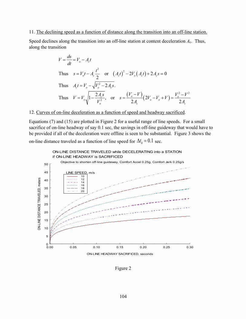
104

11. The declining speed as a function of distance along the transition into an off-line station.

Speed declines along the transition into an off-line station at content deceleration Ac. Thus, along the transition

( ) ( )

( ) ( )

22

2

2 2

2

Thus or 2 2 02

Thus 2 .

2Thus 1 , or 22 2

o c

o c c o c c

c o o c

oc oo o o

o c c

dsV V A tdt

ts V t A A t V A t A s

A t V V A s

V VA s V VV V s V V VV A A

= = −

= − − + =

= − −

− −= − = − + =

12. Curves of on-line deceleration as a function of speed and headway sacrificed.

Equations (7) and (15) are plotted in Figure 2 for a useful range of line speeds. For a small sacrifice of on-line headway of say 0.1 sec, the savings in off-line guideway that would have to be provided if all of the deceleration were offline is seen to be substantial. Figure 3 shows the on-line distance traveled as a function of line speed for 0.1ht∆ = sec.

Figure 2

0.00 0.05 0.10 0.15 0.20 0.25 0.30

ON-LINE HEADWAY SACRIFICED, seconds

0

5

10

15

20

25

30

35

40

45

50

ON-L

INE

DIST

ANCE

TRA

VELE

D, m

eter

s 101214161820

ON-LINE DISTANCE TRAVELED while DECELERATING into a STATIONif ON-LINE HEADWAY is SACRIFICED

Objective to shorten off-line guideway, Comfort Accel 0.25g, Comfort Jerk 0.25g/s

LINE SPEED, m/s

105

Figure 3

8 10 12 14 16 18 20 22 24 26 28 30

SPEED, meters/second

0

10

20

30

40

50

60

ON-L

INE

DIST

ANCE

, met

ers

ON-LINE DISTANCE TRAVELED while DECELERATING into a STATION if 0.1 sec of ON-LINE HEADWAY is SACRIFICED

106

Encoder Calibration

When using encoders on the wheels of our ITNS vehicles to measure distance and speed, the distance traveled per pulse is

Distance per Pulse / RewD

Pulses vπ

=

in which wD is the diameter of the wheel, which with compliant tires is dependent on the weight on the wheel, and / RePulses v is the number of distance steps sensed by the digital encoder per revolution of the wheel, currently 4096.

By measuring the gross weight of the vehicle, the correct wheel diameter can be recorded in the on-board computer, but we must assume that there will be a residual error to be corrected. It can be corrected by sensing a fixed distance as the vehicle leaves the station by means of wayside Hall detectors.

A sudden step in the distance parameter also occurs at each line-to-line branch point. Distance in a network is taken as a negative number that reaches zero at the branch point, and at that point is set to the negative distance to the next line-to-line branch point.

The correction in these two cases is suddenly applied the control system by the code shown in red in the following program, in which the procedure has been tested.

Public Class VehicleControl 'This program VehicleControl simulates the operation of the ITNS vehicle controller 'Units are MKS 'Steps in program: ' Start with given speed V0 and acceleration A0 ' Command Ac(t) and Vc(t) for a maneuver from given A0 and V0 ' Maneuver 0 => Maintain command speed ' Maneuver 1 => Decelerate to stop in x meters ' Maneuver 2 => Change speed to x meters/sec in minimum time ' Maneuver 3 => Slip x meters while going to line speed VL ' Obtain actual distance X(t) and speed V(t) via encoders and subtract to give ' dX = Xc - Xe, dV = Vc - Ve ' Form thrust command Tc = Gp * dX + Gv * dV ' where Gp = mc * Omega.n^2 * (1 - Beta) ' Gv = mc * Omega.n * (.5 * Beta / Zeta + 2 * Zeta * (1 - Beta)) ' mc = best estimate of vehicle mass ' Zeta = damping ratio ' Beta = dimensionless factor between 0 and 1 ' Tau = motor time constant ' Omega.n = .5 * Beta / (Zeta * Tau) = radial frequency of controller ' ' Model motor as Tau * dTh/dt + Thrust = Tc ' Model vehicle as m * dV/dt = Thrust - Drag ' Model Drag = c.air * V^2 + m * g * (aRoad + bRoad * V) '------------------------

107

'System constants Public g As Double = 9.80665 'acceleration of gravity, m/s^2 Public Jcomfort As Double = 0.25 * g 'comfort jerk, m/s^2 Public Acomfort As Double = 0.2 * g 'comfort acceleration, m/s^2 Public Ar As Double = 0.75 * Acomfort 'reduced acceleration for slip maneuvers, m/s^2 Public dVr As Double = Ar ^ 2 / Jcomfort 'speed increment, m/s Public tJ As Double = Acomfort / Jcomfort 'jerk time constant, s Public VL As Single = 15 'line speed, m/s Public Vs As Double = 7 'station speed, m/s Public Vmin As Double = VL / 2 'minimum speed for slip maneuvers, m/s Public dt As Double = 0.00001 'computation-time interval, s Public t As Double 'running time, s Public Tm, Dm As Double 'maneuver time, distance 'Vehicle parameters Public m As Double = 700 'actual vehicle mass, kg Public aRoad As Double = 0.005 'road resistance per unit weight Public bRoad As Double = 0.0005 'road resistance per unit weight/speed Public Rho As Double = 1.2 'air density, kg/m^3 Public CdA As Double = 8 'effective frontal area, m^2 Public cAir As Double = 0.5 * Rho * CdA 'air drag per unit speed^2 'Controller parameters Public dtc As Double = 0.005 'time interval between control updates, s Public dVe As Double = 0.0001 'for brake control Public Tau As Double = 0.1 'thruster lag time, s Public mc As Double = 900 'vehicle mass used in control system, kg Public Zeta As Double = 0.6 'dimensionless damping constant Public Beta As Double = 0.65 'dimensionless constant between 0 and 1 Public OmegaN As Double = Beta / (2 * Zeta * Tau) 'controller radial frequency, rad/s Public Gp As Double = mc * OmegaN ^ 2 * (1 - Beta) 'position gain Public Gv As Double = mc * OmegaN * (0.5 * Beta / Zeta + 2 * Zeta * (1 - Beta)) 'speed gain Public Dw As Double = 13.25 / 12 * 0.3048 'encoder wheel diameter, m Public PulsesPerRev As Integer = 4096 'pulses per revolution of the wheel Public dXenc As Double = Math.PI * Dw / PulsesPerRev 'encoder step, m Public Bm As Double = 0.2 * m * g 'initial braking rate, N Public V0 As Double 'speed at t = 0 Public A0 As Double 'acceleration at t = 0 Public t1, t2, t3, t4, t5, t6, t7, t8 As Double Public A1, A2, A3, A4, A5, A6, dV0 As Double Public Jerk01, Jerk12, Jerk23, Jerk34 As Double Public V1, V2, V3, V4, V5, V6, V7 As Double Public x1, x2, x3, x4, X5, X6, X7, X8 As Double Public Ac, Vc, Xc As Double 'command acceleration, speed, distance Public Vfinal, Dstop, Slip As Double 'input parameter for maneuver 2,3,4

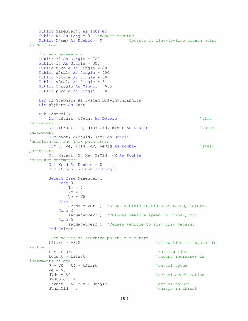
108

Public ManeuverNo As Integer Public Ne As Long = 0 'encoder counter Public Xjump As Double = 0 'Occures at line-to-line branch point in Maneuver 0 'Screen parameters Public Y0 As Single = 720 Public T0 As Single = 300 Public tScale As Single = 80 Public aScale As Single = 400 Public vScale As Single = 30 Public xScale As Single = 5 Public Thscale As Single = 0.5 Public pScale As Single = 20 Dim objGraphics As System.Drawing.Graphics Dim objFont As Font Sub Control() Dim tStart, tCount As Double 'time parameters Dim Thrust, Tc, dThdtOld, dThdt As Double 'thrust parameters Dim dVdt, dVdtOld, Jerk As Double 'acceleration and jerk parameters Dim V, Ve, Vold, dV, VeOld As Double 'speed parameters Dim Xstart, X, Xe, XeOld, dX As Double 'distance parameters Dim Xend As Double = 0 Dim xGraph, yGraph As Single Select Case ManeuverNo Case 0 Tm = 5 Ac = 0 Vc = V0 Case 1 setManeuver1() 'Stops vehicle in distance Dstop, meters. Case 2 setManeuver2() 'Changes vehicle speed to Vfinal, m/s Case 3 setManeuver3() 'Causes vehicle to slip Slip meters. End Select 'Set values at starting point, t = tStart tStart = -2.5 'allow time for system to settle t = tStart 'running time tCount = tStart 'tcount increases in increments of dtc V = V0 + A0 * tStart 'actual speed Ve = V0 dVdt = A0 'actual acceleration dVdtOld = A0 Thrust = A0 * m + Drag(V) 'actual thrust dThdtOld = 0 'change in thrust

109

Xstart = tStart * (V0 + 0.5 * A0 * tStart) 'distance, so X = 0 when t = 0 X = Xstart 'actual distance at start XeOld = Xstart - V0 * dtc 'previous measured distance Jerk = 0 objFont = New System.Drawing.Font("Arial", 40) objGraphics = Me.CreateGraphics objGraphics.DrawLine(Pens.White, T0, Y0, T0, 0) objGraphics.DrawLine(Pens.White, T0, Y0, 1500, Y0) objGraphics.DrawLine(Pens.Red, T0, Y0 - vScale * VL, 1500, Y0 - vScale * VL) For i As Integer = 1 To 30 objGraphics.DrawLine(Pens.White, T0 + tScale * i, Y0, T0 + tScale * i, Y0 - 10) Next objGraphics.DrawString(" Command Acceleration ", Me.Font, System.Drawing.Brushes.White, 500, 30) objGraphics.DrawString(" Command Speed ", Me.Font, System.Drawing.Brushes.Pink, 500, 50) objGraphics.DrawString(" Command Distance ", Me.Font, System.Drawing.Brushes.Fuchsia, 500, 70) objGraphics.DrawString(" Acceleration ", Me.Font, System.Drawing.Brushes.Yellow, 500, 90) objGraphics.DrawString(" Speed ", Me.Font, System.Drawing.Brushes.Red, 500, 110) objGraphics.DrawString(" Distance ", Me.Font, System.Drawing.Brushes.Turquoise, 500, 130) objGraphics.DrawString(" Thrust ", Me.Font, System.Drawing.Brushes.Gray, 500, 150) objGraphics.DrawString(" Acceleration Power ", Me.Font, System.Drawing.Brushes.GreenYellow, 500, 170) objGraphics.DrawString(" Jerk ", Me.Font, System.Drawing.Brushes.Goldenrod, 500, 190) Do xGraph = T0 + tScale * t yGraph = Y0 - aScale * Ac objGraphics.FillEllipse(Brushes.White, xGraph, yGraph, 2, 2) yGraph = Y0 - vScale * Vc objGraphics.FillEllipse(Brushes.Pink, xGraph, yGraph, 2, 2) yGraph = Y0 - xScale * Xc objGraphics.FillEllipse(Brushes.Fuchsia, xGraph, yGraph, 2, 2) yGraph = Y0 - aScale * dVdt objGraphics.FillEllipse(Brushes.Yellow, xGraph, yGraph, 2, 2) yGraph = Y0 - vScale * V objGraphics.FillEllipse(Brushes.Red, xGraph, yGraph, 2, 2) yGraph = Y0 - xScale * X objGraphics.FillEllipse(Brushes.Turquoise, xGraph, yGraph, 2, 2) yGraph = Y0 - Thscale * (Thrust - 500) objGraphics.FillEllipse(Brushes.Gray, xGraph, yGraph, 2, 2) yGraph = Y0 - pScale * dVdt * V 'acceleration power objGraphics.FillEllipse(Brushes.GreenYellow, xGraph, yGraph, 2, 2) yGraph = Y0 - 0.01 * aScale * Jerk

110

'objGraphics.FillEllipse(Brushes.Goldenrod, xGraph, yGraph, 2, 2) 'Simulate digital encoder Xe = Encoder(X, Xstart) 'measured position 'Enter the on-board computer If t >= tCount Then tCount = tCount + dtc If t < 0 Then Ac = A0 Vc = V0 + A0 * t Xc = t * (V0 + A0 * t / 2) End If Select Case ManeuverNo Case 0 If t >= 0 Then Xjump = -500 Xc = Xjump + V0 * t If t < dtc Then Xstart = Xstart + Xjump Xe = Xe + Xjump XeOld = XeOld + Xjump X = X + Xjump End If End If Case 1 If t > 0 Then runManeuver1() 'output Ac, Vc, Xc End If Case 2 If t > 0 Then runManeuver2() 'output Ac, Vc, Xc End If Case 3 If t > 0 Then runManeuver3() 'output Ac, Vc, Xc End If End Select Ve = (Xe - XeOld) / dtc 'differentiate to measure speed VeOld = Ve XeOld = Xe dX = Xc - Xe 'command position - measured position dV = Vc - Ve 'command speed - measured speed Tc = Gp * dX + Gv * dV 'command thrust If Vfinal < 0.01 And Ve < dVe Then Tc = 0 End If 'Simulate thruster as first-order lag dThdt = (Tc - Thrust) / Tau 'time rate of change of thrust Thrust = Thrust + 0.5 * dt * (3 * dThdt - dThdtOld) 'actual thrust dThdtOld = dThdt 'If ManeuverNo = 1 And (t >= Tm Or V < 0) Then Thrust = 0

111

'Simulate vehicle dynamics dVdt = (Thrust - Drag(V)) / m 'acceleration Jerk = (dVdt - dVdtOld) / dt If Vfinal < 0.01 And Ve < dVe Then dVdt = dVdt - Brake(V) / m End If Vold = V V = V + 0.5 * dt * (3 * dVdt - dVdtOld) 'speed dVdtOld = dVdt X = X + 0.5 * dt * (V + Vold) 'position If t >= Tm And Xend = 0 Then Xend = X End If t = t + dt Application.DoEvents() Loop Until t > 1.1 * Tm objGraphics.DrawString(" The Maneuver Time is " & FormatNumber(CSng(Tm), 2) & " sec", Me.Font, _ System.Drawing.Brushes.White, 900, 200) If ManeuverNo = 1 Then 'Stop in given distance Dstop objGraphics.DrawString(" The commanded Maneuver Distance is " & FormatNumber(CSng(Dstop), 2) & " meters", Me.Font, _ System.Drawing.Brushes.White, 900, 220) objGraphics.DrawString(" The actual distance at maneuver end is " & FormatNumber(CSng(Xend), 2) & " meters", Me.Font, _ System.Drawing.Brushes.White, 900, 240) ElseIf ManeuverNo = 2 Then 'Change speed to Vfinal objGraphics.DrawString(" The commanded Final Speed is " & FormatNumber(CSng(Vfinal), 2) & " m/s", Me.Font, _ System.Drawing.Brushes.White, 900, 220) objGraphics.DrawString(" The actual Final Speed is " & FormatNumber(CSng(V), 2) & " m/s", Me.Font, _ System.Drawing.Brushes.White, 900, 240) ElseIf ManeuverNo = 3 Then objGraphics.DrawString(" The commanded Slip Distance is " & FormatNumber(CSng(Slip), 2) & " meters", Me.Font, _ System.Drawing.Brushes.White, 900, 220) objGraphics.DrawString(" The actual slip Distance is " & FormatNumber(CSng(VL * Tm - Dm), 2) & " meters", Me.Font, _ System.Drawing.Brushes.White, 900, 240) End If objGraphics.Dispose() objFont.Dispose() End Sub Function Brake(ByVal V As Double) As Double Dim dBm As Double dBm = 0.002 * m * g If ManeuverNo = 1 Then If t >= Tm Or V < 0 Then Bm = Bm - dBm

112

If Bm < 0 Then Bm = 0 If V > 0 Then Brake = Bm ElseIf V < 0 Then Brake = -Bm Else Brake = 0 End If Else Brake = 0 End If Else Brake = 0 End If End Function Function Drag(ByVal V As Double) As Double Dim D As Double D = Math.Sign(V) * cAir * V ^ 2 + m * g * (bRoad * V + Math.Sign(V) * aRoad) If ManeuverNo = 1 And V < 0.1 Then D = 0 Drag = D End Function Function Encoder(ByVal X As Double, ByVal Xstart As Double) As Double 'STATIC If X >= Xstart + (Ne + 0.5) * dXenc Then Ne = Ne + 1 Encoder = Ne * dXenc + Xstart End Function Sub runManeuver1() Dim Jerk As Double If t < t2 Then Jerk = -Math.Sign(dV0) * Jcomfort State(t, Jerk, A0, V0, 0) 'Ac = command acceleration ElseIf t < t3 Then 'Vc = command speed Jerk = 0 'Xc = command distance travelled State(t - t2, Jerk, A2, V2, x2) ElseIf t < t4 Then Jerk = Math.Sign(dV0) * Jcomfort State(t - t3, Jerk, A2, V3, x3) ElseIf t < t5 Then Jerk = 0 State(t - t4, Jerk, 0, V4, x4) ElseIf t < t6 Then Jerk = -Jcomfort State(t - t5, Jerk, 0, V4, X5) ElseIf t < t7 Then Jerk = 0 State(t - t6, Jerk, A6, V6, X6) ElseIf t < t8 Then Jerk = Jcomfort State(t - t7, Jerk, A6, V7, X7) ElseIf t >= t8 Then Jerk = 0 State(t - t8, Jerk, 0, 0, X8) End If

113

End Sub Sub runManeuver2() Dim AcOld As Double AcOld = Ac If t < t1 Then State(t, Jerk01, A0, V0, 0) 'Ac is command acceleration ElseIf t < t2 Then 'Vc is command speed State(t - t1, Jerk12, A1, V1, x1) ElseIf t < t3 Then State(t - t2, Jerk23, A2, V2, x2) ElseIf t < t4 Then State(t - t3, Jerk34, A3, V3, x3) Else State(t - t4, 0, 0, Vfinal, x4) End If End Sub Sub runManeuver3() Dim Jerk, A1a, V1a As Double If t < t1 Then Jerk = -Jcomfort State(t, Jerk, A0, V0, 0) ElseIf t < t2 Then Jerk = -Jcomfort If A0 >= 0 Then A1a = A1 V1a = V1 Else A1a = A0 V1a = V0 End If State(t - t1, Jerk, A1a, V1a, x1) ElseIf t < t3 Then 'Vc is command speed Jerk = 0 'Xc is command distance State(t - t2, Jerk, A2, V2, x2) ElseIf t < t4 Then Jerk = Jcomfort State(t - t3, Jerk, A2, V3, x3) ElseIf t < t5 Then Jerk = 0 State(t - t4, Jerk, A4, V4, x4) ElseIf t < t6 Then Jerk = Jcomfort State(t - t5, Jerk, A5, V5, X5) ElseIf t < t7 Then Jerk = 0 State(t - t6, Jerk, A6, V6, X6) ElseIf t < t8 Then Jerk = -Jcomfort State(t - t7, Jerk, A6, V7, X7) Else Jerk = 0 State(t - t8, Jerk, 0, VL, X8) End If End Sub

114

'This maneuver stops a vehicle in a given distance Sub setManeuver1() Dim Tmin, Dmin As Double Dim dt01, dt12, dt23, dt34, dt45, dt56, dt67, dt78 As Double Dim dx01, dx12, dx23, dx34, dx45, dx56, dx67, dx78, dx14, dx58 As Double Dim Dbnd, b, dV, Dold, V5 As Double Vfinal = 0 If Math.Abs(A0) > Acomfort Then A0 = Math.Sign(A0) * Acomfort 'can't exceed Acomfort 'Condition of negative V not operational on deceleration to stop If A0 < 0 And V0 < A0 ^ 2 / Jcomfort Then V0 = A0 ^ 2 / Jcomfort dV0 = V0 + A0 ^ 2 / 2 / Jcomfort - Vs 'indicator 'Calculate minimum stopping time and distance V1 = V0 + A0 ^ 2 / 2 / Jcomfort If V1 >= A0 ^ 2 / Jcomfort Then Tmin = V1 / Acomfort + Acomfort / Jcomfort ElseIf V1 >= 0 Then Tmin = 2 * Math.Sqrt(V1 / Jcomfort) Else Tmin = 0 End If Dmin = 0.5 * V1 * Tmin + (A0 / Jcomfort) * (V0 + A0 ^ 2 / 3 / Jcomfort) dt01 = Math.Sign(dV0) * A0 / Jcomfort V1 = V0 + Math.Sign(dV0) * A0 ^ 2 / 2 / Jcomfort dx01 = (A0 / Jcomfort) * (Math.Sign(dV0) * V0 + A0 ^ 2 / 3 / Jcomfort) If Dstop < Dmin Then objGraphics.DrawString(" The Minimum Maneuver Distance is " & FormatNumber(Dmin, 2) & " meters", Me.Font, _ System.Drawing.Brushes.White, 900, 220) End If V4 = Vs 'if V0 < Vs V4 may later be reduced below Vs If Math.Abs(V4 - V1) >= Acomfort * tJ Then A2 = -Math.Sign(dV0) * Acomfort ElseIf Math.Abs(V4 - V1) > 0 Then A2 = -Math.Sign(dV0) * Math.Sqrt(Jcomfort * Math.Abs(V4 - V1)) Else A2 = 0 End If If V4 >= Acomfort * tJ Then A6 = -Acomfort ElseIf V4 > 0 Then A6 = -Math.Sqrt(Jcomfort * V4) 'V4 > 0 if there is any maneuver at all Else A6 = 0 End If

115

'Calculate boundry stopping distance if dx45 = 0 and V4 = Vs If A2 <> 0 Then dx14 = 0.5 * (V4 + V1) * ((V4 - V1) / A2 - Math.Sign(dV0) * A2 / Jcomfort) Else dx14 = 0 End If If A6 <> 0 Then dx58 = -0.5 * V4 * (V4 / A6 + A6 / Jcomfort) Else dx58 = 0 Dbnd = dx14 + dx58 + dx01 A4 = 0 'true always A5 = A4 'true always If Dstop >= Dbnd Then dx45 = Dstop - Dbnd Else dx45 = 0 If dV0 > 0 And Dstop < Dbnd Then 'in these cases don't slow down near Vs b = (Jcomfort / V1) * (Dstop - (A0 / Jcomfort) * (V0 + A0 ^ 2 / 3 / Jcomfort)) A2 = -b + Math.Sqrt(b ^ 2 - V1 * Jcomfort) 'reduced deceleration Else dV = 0.005 'increment in which V4 is reduced if need be Do Dold = Dbnd 'used in Newtonian intepolation after do-loop 'distance from point 1 to 4: If A2 <> 0 Then dx14 = 0.5 * (V4 + V1) * ((V4 - V1) / A2 - Math.Sign(dV0) * A2 / Jcomfort) Else dx14 = 0 End If 'distance from point 5 to 8: If A6 <> 0 Then dx58 = -0.5 * V4 * (V4 / A6 + A6 / Jcomfort) Else dx58 = 0 End If 'boundry distance above which dx45 > 0 Dbnd = dx14 + dx58 + dx01 If Dbnd < Dstop Then 'if true do-loop is finished Exit Do Else V4 = V4 - dV 'step V4 down until Dbnd = Dstop If V4 < dV Then 'this condition should never occur V4 = dV Exit Do End If End If If Math.Abs(V4 - V1) >= Acomfort * tJ Then 'recalculate A2 with lower V4 A2 = -Math.Sign(dV0) * Acomfort

116

ElseIf Math.Abs(V4 - V1) > 0 Then A2 = -Math.Sign(dV0) * Math.Sqrt(Jcomfort * Math.Abs(V4 - V1)) Else A2 = 0 End If If V4 > Acomfort * tJ Then A6 = -Acomfort ElseIf V4 > 0 Then A6 = -Math.Sqrt(Jcomfort * V4) Else A6 = 0 End If Loop V4 = V4 + dV * (Dstop - Dbnd) / (Dold - Dbnd) 'Newtonian interpolation If V4 < dV Then V4 = dV If Math.Abs(V4 - V1) >= Acomfort * tJ Then 'recalculation of A2 with final V4 A2 = Math.Sign(Vs - V0) * Acomfort ElseIf Math.Abs(V4 - V1) > 0 Then A2 = Math.Sign(Vs - V0) * Math.Sqrt(Jcomfort * Math.Abs(V4 - V1)) Else A2 = 0 End If If V4 > Acomfort * tJ Then A6 = -Acomfort ElseIf V4 > 0 Then A6 = -Math.Sqrt(Jcomfort * V4) Else A6 = 0 End If End If End If dt12 = Math.Abs(A2) / Jcomfort V2 = V1 + dt12 * A2 / 2 dx12 = dt12 * (V1 + dt12 * A2 / 6) If dV0 >= 0 And Dstop < Dbnd Then 'special case of no slowdown at Vs dt34 = -A2 / Jcomfort V3 = -dt34 * A2 / 2 dx34 = dt34 * (V3 + dt34 * A2 / 3) If A2 <> 0 Then dt23 = (V3 - V2) / A2 Else dt23 = 0 dx23 = dt23 * (V2 + dt23 * A2 / 2) dt45 = 0 dx45 = 0 dt56 = 0 dx56 = 0 dt67 = 0

117

dx67 = 0 dt78 = 0 dx78 = 0 Else 'all other cases dt34 = -Math.Sign(dV0) * A2 / Jcomfort V3 = V4 - dt34 * A2 / 2 dx34 = dt34 * (V3 + dt34 * A2 / 3) If A2 <> 0 Then dt23 = (V3 - V2) / A2 Else dt23 = 0 dx23 = dt23 * (V2 + dt23 * A2 / 2) dt45 = dx45 / Vs V5 = V4 dt56 = -A6 / Jcomfort V6 = V5 + dt56 * A6 / 2 dx56 = dt56 * (V5 + dt56 * A6 / 6) dt78 = -A6 / Jcomfort V7 = -dt78 * A6 / 2 dx78 = dt78 * (V7 + dt78 * A6 / 3) If A6 <> 0 Then dt67 = (V7 - V6) / A6 Else dt67 = 0 dx67 = dt67 * (V6 + dt67 * A6 / 2) End If t1 = dt01 'record all times where jerk change t2 = t1 + dt12 t3 = t2 + dt23 t4 = t3 + dt34 t5 = t4 + dt45 t6 = t5 + dt56 t7 = t6 + dt67 t8 = t7 + dt78 Tm = t8 'maneuver time x1 = dx01 'record all distances where jerk changes x2 = x1 + dx12 x3 = x2 + dx23 x4 = x3 + dx34 X5 = x4 + dx45 X6 = X5 + dx56 X7 = X6 + dx67 X8 = X7 + dx78 Dm = X8 'maneuver distance End Sub 'This maneuver changes speed to speed Vfinal Sub setManeuver2() 'This maneuver changes speed to Vfinal Dim Alpha, Beta, dVc, dVo As Double Dim Jc, Jn As Double Dim Vb, Va As Double Dim dt01, dt12, dt23, dt34, dx01, dx12, dx23, dx34, Dm As Double Dim Flag1, Flag2 As Integer Alpha = 0.5

118

Beta = 0.5 dVc = Acomfort ^ 2 / 2 / Jcomfort dVo = A0 ^ 2 / 2 / Jcomfort Jc = Jcomfort Vb = CSng(Beta ^ 2) * dVc Va = Alpha * VL 'boundary speed, above which A < Acomfort Jn = CSng((1 - Beta ^ 2) * Acomfort ^ 2 / 2 / (VL - Va - Beta ^ 2 * dVc)) 'Treat small changes in speed separately: Flag1 = 0 If Math.Abs(Vfinal - V0) + dVo <= 2 * dVc Then If V0 + Math.Sign(A0) * dVo >= Vfinal Then Jerk01 = -Jc Jerk34 = Jc A1 = -CSng(Math.Sqrt(Jc * (V0 + dVo - Vfinal))) V1 = (V0 + dVo + Vfinal) / 2 Flag1 = 1 Else Jerk01 = Jc Jerk34 = -Jc A1 = CSng(Math.Sqrt(Jc * (Vfinal - V0 + dVo))) V1 = (Vfinal + V0 - dVo) / 2 Flag1 = 2 End If A2 = A1 A3 = A1 V2 = V1 V3 = V1 End If Flag2 = 0 If Flag1 = 0 Then If Vfinal > Va Then If V0 + Math.Sign(A0) * dVo > Vfinal Then Jerk01 = -Jc Jerk12 = 0 'dt12 = 0 Jerk23 = -Jn Jerk34 = Jc V1 = (V0 + dVo - dVc - Va * Jn / Jc) / (1 - Jn / Jc) A1 = -CSng(Math.Sqrt(Acomfort ^ 2 - 2 * Jn * (V1 - Va))) A2 = A1 V2 = V1 V3 = (Vfinal + dVc + Va * Jn / Jc) / (1 + Jn / Jc) A3 = -CSng(Math.Sqrt(Acomfort ^ 2 - 2 * Jn * (V3 - Va))) If A0 < 0 And V1 > V0 Then A1 = A0 V1 = V0 A2 = A1 V2 = V1 Jerk23 = -CSng(A3 ^ 2 - A2 ^ 2) / 2 / (V2 - V3) End If Flag2 = 1 Else 'V0 + Math.Sign(A0) * dVo <= Vfinal If V0 - dVo + dVc > Va Then

119

Jerk01 = Jc Jerk12 = 0 Jerk23 = -Jn Jerk34 = -Jc V1 = (V0 - dVo + dVc + Va * Jn / Jc) / (1 + Jn / Jc) A1 = CSng(Math.Sqrt(Acomfort ^ 2 - 2 * Jn * (V1 - Va))) A2 = A1 V2 = V1 V3 = (Vfinal - dVc - Va * Jn / Jc) / (1 - Jn / Jc) A3 = CSng(Math.Sqrt(Acomfort ^ 2 - 2 * Jn * (V3 - Va))) If A1 < A0 Then A1 = A0 V1 = V0 A2 = A1 V2 = V1 Jerk23 = -CSng(A2 ^ 2 - A3 ^ 2) / 2 / (V3 - V2) End If Flag2 = 2 Else 'V0 - dVo + dVc <= Va Jerk01 = Jc Jerk12 = 0 Jerk23 = -Jn Jerk34 = -Jc A1 = Acomfort A2 = Acomfort V1 = V0 - dVo + dVc V2 = Va V3 = (Vfinal - dVc - Va * Jn / Jc) / (1 - Jn / Jc) A3 = CSng(Math.Sqrt(Acomfort ^ 2 - 2 * Jn * (V3 - Va))) If V3 < Va Then A3 = Acomfort V3 = Vfinal - CSng(A3 ^ 2) / 2 / Jc V2 = V3 End If If V1 > V2 Then V2 = V1 Jerk23 = -CSng(A2 ^ 2 - A3 ^ 2) / 2 / (V3 - V2) End If Flag2 = 3 End If End If Else 'Vfinal <= Va) If V0 + Math.Sign(A0) * dVo > Vfinal Then If V0 + dVo - dVc > Va Then Jerk01 = -Jc Jerk12 = -Jn 'dt12 = 0 Jerk23 = 0 Jerk34 = Jc V1 = (V0 + dVo - dVc - Va * Jn / Jc) / (1 - Jn / Jc) A1 = -CSng(Math.Sqrt(Acomfort ^ 2 - 2 * Jn * (V1 - Va))) A2 = -Acomfort A3 = -Acomfort V2 = Va

120

If A1 > A0 Then A1 = A0 V1 = V0 Jerk12 = -CSng(A2 ^ 2 - A1 ^ 2) / 2 / (V1 - V2) End If V3 = Vfinal + dVc If V3 > V2 Then V2 = V3 Jerk12 = -CSng(Acomfort ^ 2 - A1 ^ 2) / 2 / (V1 - V2) End If Flag2 = 4 Else 'V0 + dVo - dVc<= Va Jerk01 = -Jc Jerk12 = 0 'dt12 = 0 Jerk23 = 0 Jerk34 = Jc A1 = -Acomfort A2 = -Acomfort A3 = -Acomfort V1 = V0 + dVo - dVc V2 = V1 V3 = Vfinal + dVc Flag2 = 5 End If Else 'V0 + Math.Sign(A0) * dVo < Vfinal Jerk01 = Jc Jerk12 = 0 Jerk23 = 0 Jerk34 = -Jc A1 = Acomfort A2 = Acomfort A3 = Acomfort V1 = V0 - dVo + dVc V2 = V1 V3 = Vfinal - dVc Flag2 = 6 End If End If End If dt01 = (A1 - A0) / Jerk01 If Math.Abs(Jerk12) > 0 Then dt12 = (A2 - A1) / Jerk12 Else If Math.Abs(A2) > 0 Or Math.Abs(A1) > 0 Then dt12 = 2 * (V2 - V1) / (A2 + A1) Else dt12 = 0 End If End If If Math.Abs(Jerk23) > 0 Then dt23 = (A3 - A2) / Jerk23 Else If Math.Abs(A3) > 0 Or Math.Abs(A2) > 0 Then dt23 = 2 * (V3 - V2) / (A3 + A2) Else

121

dt23 = 0 End If End If dt34 = -A3 / Jerk34 dx01 = dt01 * (V0 + dt01 * (2 * A0 + A1) / 6) dx12 = dt12 * (V1 + dt12 * (2 * A1 + A2) / 6) dx23 = dt23 * (V2 + dt23 * (2 * A2 + A3) / 6) dx34 = dt34 * (V3 + dt34 * A3 / 3) t1 = dt01 t2 = t1 + dt12 t3 = t2 + dt23 t4 = t3 + dt34 'Maneuver time Tm = t4 x1 = dx01 x2 = x1 + dx12 x3 = x2 + dx23 x4 = x3 + dx34 Dm = dx01 + dx12 + dx23 + dx34 'Maneuver distance End Sub 'This maneuver causes vehicle to slip amount Slip before reaching VL Sub setManeuver3() Dim Smin, S01, DV, V1r As Double Dim dt01, dt12, dt23, dt34, dt45, dt56, dt67, dt78 As Double Dim dx01, dx12, dx23, dx34, dx45, dx56, dx67, dx78 As Double Dim Sbnd1, Sbnd2, Sbnd3, Sbnd4, b, c, slp, SlipError, Va, V4a As Double Dim dV0, V4previous, Sprevious, V4p, Sp As Double Dim i, Flag As Integer 'Calculate point 1 at which A1 = 0 for the purpose of calculating boundaries dt01 = A0 / Jcomfort '< 0 if A0 < 0, which subtracts S01 V1 = V0 + dt01 * A0 / 2 dx01 = dt01 * (V0 + dt01 * A0 / 3) S01 = VL * dt01 - dx01 'slip during interval 0-1, > 0 if A0 > 0, < 0 if A0 < 0 'Calculate V4 in all cases except between Sbnd3 and Sbnd4, where calculate A1 dx45 = 0 'cases when not zero will be calculated A1 = 0 A5 = 0 dV0 = A0 ^ 2 / Jcomfort If V0 = VL And A0 = 0 Then DV = VL - Vmin Sbnd1 = DV * (DV / Ar + Ar / Jcomfort) 'DV > dVr always Sbnd2 = 2 * dVr * Ar / Jcomfort Sbnd3 = 0 If Slip >= Sbnd1 Then dx45 = (Slip - Sbnd1) * Vmin / (VL - Vmin) V4 = Vmin ElseIf Slip > 0 Then dx45 = 0

122

If Slip >= Sbnd2 Then V4 = VL + 0.5F * dVr - Math.Sqrt(Ar * Slip + 0.25 * dVr ^ 2) Else V4 = VL - (Jcomfort * Slip ^ 2 / 4) ^ (1 / 3) End If Else V4 = VL End If V5 = V4 Else Sbnd1 = S01 + SlipV4(Vmin) 'boundary when V4=Vmin and dx45=0 If V1 - dVr > Vmin Then Sbnd2 = S01 + SlipV4(V1 - dVr) 'boundary when V4=V1-dVr Else Sbnd2 = Sbnd1 End If If A0 >= 0 Then Sbnd3 = S01 + SlipV4(V1) 'boundary when V4 = V1 Sbnd4 = SlipA1(A0, A6) Smin = Sbnd4 Else Sbnd3 = S01 + SlipV4(V1 - dV0) 'boundary when V4 = V1 Sbnd4 = Sbnd3 Smin = Sbnd3 End If If Slip < Smin Then Slip = Smin 'can't go lower than Smin 'Calculate V4: If Slip >= Sbnd1 Then dx45 = (Slip - Sbnd1) * Vmin / (VL - Vmin) V4 = Vmin ElseIf Slip >= Sbnd2 Then 'increase V4 above Vmin b = VL + 0.5F * dVr c = (VL - 0.5 * V1) * (V1 + dVr) + 0.5 * VL * (VL + dVr) V4 = b - Math.Sqrt(b ^ 2 - c + Ar * (Slip - S01)) ElseIf Slip >= Sbnd3 Then 'Find V4 by iteration V1r = V1 - dVr If A0 >= 0 Then V4 = V1 - dVr * (Slip - Sbnd3) / (Sbnd2 - Sbnd3) slp = S01 + SlipV4(V4) i = 0 Flag = 0 Do V4previous = V4 Sprevious = slp If slp >= Slip Then If Slip > Sbnd3 Then V4 = V1 + (V1 - V4) * (Slip - Sbnd3) / (slp - Sbnd3) Else V4 = V1 Exit Do End If

123

Else V4 = V1r + (V4 - V1r) * (Sbnd2 - Slip) / (Sbnd2 - slp) End If slp = S01 + SlipV4(V4) If Math.Sign(Slip - slp) + Math.Sign(Slip - Sprevious) = 0 Then Exit Do i = i + 1 If Math.Abs(slp - Slip) < 0.001 Then Flag = 1 Exit Do End If Loop If Flag = 0 And Math.Sign(Slip - slp) + Math.Sign(Slip - Sprevious) = 0 Then Do V4p = V4 Sp = slp V4 = ((Slip - Sprevious) * V4 + (slp - Slip) * V4previous) / (slp - Sprevious) slp = S01 + SlipV4(V4) V4previous = V4p Sprevious = Sp Loop Until Math.Abs(slp - Slip) < 0.001 End If Else 'A0 < 0 V4 = V1r + (dVr - dV0) * (Sbnd2 - Slip) / (Sbnd2 - Sbnd3) slp = S01 + SlipV4(V4) i = 0 If Math.Abs(slp - Slip) > 0.001 Then Do If slp >= Slip Then V4 = V4 + (V1 - dV0 - V4) * (slp - Slip) / (slp - Sbnd3) Else V4 = V1r + (V4 - V1 + dVr) * (Sbnd2 - Slip) / (Sbnd2 - slp) End If slp = S01 + SlipV4(V4) i = i + 1 Loop Until Math.Abs(slp - Slip) < 0.001 End If End If ElseIf Slip >= Sbnd4 Then 'In these cases A0 > 0 and points 1,2,3,4,5 coincide 'Calculate A1 A1 = A0 * (Sbnd3 - Slip) / (Sbnd3 - Sbnd4) 'first guess for A1 slp = SlipA1(A1, A6) i = 0 Do If slp >= Slip Then A1 = A0 - (A0 - A1) * (Slip - Sbnd4) / (slp - Sbnd4) Else A1 = A1 * (Sbnd3 - Slip) / (Sbnd3 - slp) End If

124

slp = SlipA1(A1, A6) i = i + 1 SlipError = Slip - slp Loop Until Math.Abs(SlipError) < 0.001 End If End If 'Having V4 we now can compute A2,V2,V3,A4,A5: If Slip >= Sbnd3 Then If V1 - V4 >= dVr Then A2 = -Ar ElseIf V1 - V4 > 0 Then A2 = -Math.Sqrt(Jcomfort * (V1 - V4)) If A0 < 0 And Math.Abs(V1 - V4 - dV0) < 0.000001 Then A2 = A0 End If Else A2 = 0 End If If A0 >= 0 Then dt12 = -(A2 - A1) / Jcomfort V2 = V1 + dt12 * (A2 + A1) / 2 dx12 = dt12 * (V1 + dt12 * (2 * A1 + A2) / 6) Else dt12 = -(A2 - A0) / Jcomfort V2 = V0 + dt12 * (A2 + A0) / 2 dx12 = dt12 * (V0 + dt12 * (2 * A0 + A2) / 6) dt01 = 0 dx01 = 0 End If dt34 = -A2 / Jcomfort V3 = V4 - dt34 * A2 / 2 dx34 = dt34 * (V3 + dt34 * A2 / 3) If A2 <> 0 Then dt23 = (V3 - V2) / A2 Else dt23 = 0 End If dx23 = dt23 * (V2 + dt23 * A2 / 2) A4 = 0 A5 = 0 V5 = V4 ElseIf Slip >= Sbnd4 Then 'A0 > 0 in this case dt01 = -(A1 - A0) / Jcomfort 'here A1 <= A0, jerk is negative V1 = V0 + dt01 * (A0 + A1) / 2 dx01 = dt01 * (V0 + dt01 * (2 * A0 + A1) / 6) 'points 1, 2, 3, 4, 5 coincide Va = V0 + A0 ^ 2 / 2 / Jcomfort - A1 ^ 2 / Jcomfort dt12 = 0 V2 = V1

125

dx12 = 0 dt34 = 0 V3 = V1 dx34 = 0 dt23 = 0 dx23 = 0 A2 = A1 A3 = A1 A4 = A1 A5 = A1 V4 = V1 V5 = V1 End If If Slip >= Sbnd3 Then V4a = V4 Else V4a = Va End If DV = VL - V4a If DV >= dVr Then A6 = Ar ElseIf DV > 0 Then A6 = Math.Sqrt(Jcomfort * DV) Else A6 = 0 End If dt45 = dx45 / Vmin V5 = V4 dt56 = (A6 - A5) / Jcomfort V6 = V5 + dt56 * (A5 + A6) / 2 dx56 = dt56 * (V5 + dt56 * (2 * A5 + A6) / 6) dt78 = A6 / Jcomfort V7 = VL - dt78 * A6 / 2 dx78 = dt78 * (V7 + dt78 * A6 / 3) If A6 > 0 Then dt67 = (V7 - V6) / A6 Else dt67 = 0 End If dx67 = dt67 * (V6 + dt67 * A6 / 2) 'Now compute the times at the eight points t1 = dt01 t2 = t1 + dt12 t3 = t2 + dt23 t4 = t3 + dt34 t5 = t4 + dt45 t6 = t5 + dt56

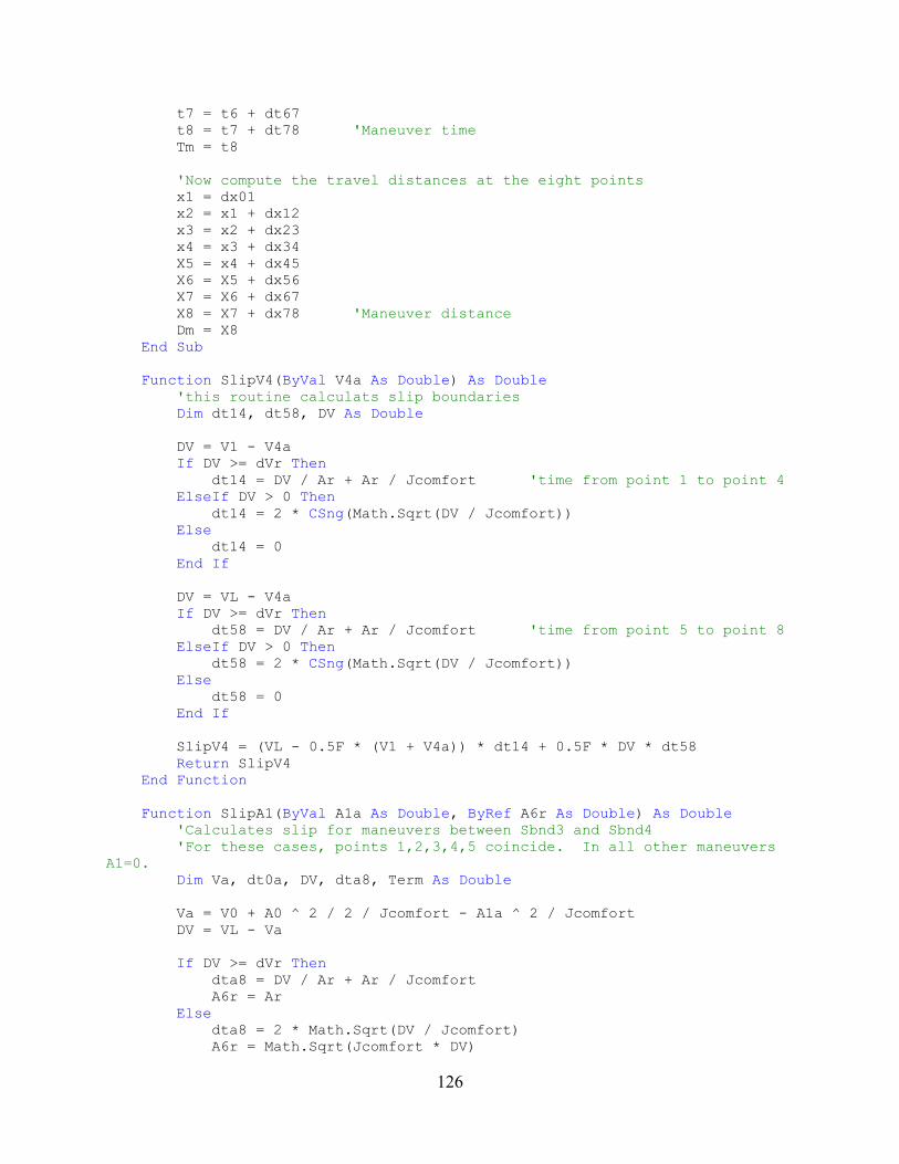
126

t7 = t6 + dt67 t8 = t7 + dt78 'Maneuver time Tm = t8 'Now compute the travel distances at the eight points x1 = dx01 x2 = x1 + dx12 x3 = x2 + dx23 x4 = x3 + dx34 X5 = x4 + dx45 X6 = X5 + dx56 X7 = X6 + dx67 X8 = X7 + dx78 'Maneuver distance Dm = X8 End Sub Function SlipV4(ByVal V4a As Double) As Double 'this routine calculats slip boundaries Dim dt14, dt58, DV As Double DV = V1 - V4a If DV >= dVr Then dt14 = DV / Ar + Ar / Jcomfort 'time from point 1 to point 4 ElseIf DV > 0 Then dt14 = 2 * CSng(Math.Sqrt(DV / Jcomfort)) Else dt14 = 0 End If DV = VL - V4a If DV >= dVr Then dt58 = DV / Ar + Ar / Jcomfort 'time from point 5 to point 8 ElseIf DV > 0 Then dt58 = 2 * CSng(Math.Sqrt(DV / Jcomfort)) Else dt58 = 0 End If SlipV4 = (VL - 0.5F * (V1 + V4a)) * dt14 + 0.5F * DV * dt58 Return SlipV4 End Function Function SlipA1(ByVal A1a As Double, ByRef A6r As Double) As Double 'Calculates slip for maneuvers between Sbnd3 and Sbnd4 'For these cases, points 1,2,3,4,5 coincide. In all other maneuvers A1=0. Dim Va, dt0a, DV, dta8, Term As Double Va = V0 + A0 ^ 2 / 2 / Jcomfort - A1a ^ 2 / Jcomfort DV = VL - Va If DV >= dVr Then dta8 = DV / Ar + Ar / Jcomfort A6r = Ar Else dta8 = 2 * Math.Sqrt(DV / Jcomfort) A6r = Math.Sqrt(Jcomfort * DV)

127

End If dt0a = (2 * A1a - A0) / Jcomfort Term = VL - V0 - (A0 ^ 2 - 2 * A0 * A1a - 2 * A1a ^ 2) / 3 / Jcomfort SlipA1 = 0.5 * DV * dta8 - dt0a * Term + A1a * (A1a / Jcomfort) ^ 2 / 3 End Function Function SlipBoundary(ByVal V1 As Double, ByVal V4 As Double, ByVal S01 As Double) As Double Dim Ar, Vb, T14, T58, Term1, Term2 As Double Ar = 0.75 * Acomfort 'reduced maximum acceleration near line speed Vb = Ar ^ 2 / Jcomfort If V1 - V4 >= Vb Then T14 = (V1 - V4) / Ar + Ar / Jcomfort 'time from point 1 to point 4 ElseIf V1 - V4 > 0 Then T14 = 2 * Math.Sqrt((V1 - V4) / Jcomfort) Else T14 = 0 End If If VL - V4 >= Vb Then T58 = (VL - V4) / Ar + Ar / Jcomfort 'time from point 5 to point 8 ElseIf VL - V4 > 0 Then T58 = 2 * Math.Sqrt((VL - V4) / Jcomfort) Else T58 = 0 End If Term1 = 0.5 * (2 * VL - V1 - V4) * T14 Term2 = 0.5 * (VL - V4) * T58 SlipBoundary = S01 + Term1 + Term2 End Function Sub State(ByVal Delt, ByVal J, ByVal Ao, ByVal Vo, ByVal Xo) Dim Delt2 As Double Delt2 = Delt * Delt / 2 Ac = Ao + J * Delt Vc = Vo + Ao * Delt + J * Delt2 Xc = Xo + Vo * Delt + Ao * Delt2 + J * Delt2 * Delt / 3 End Sub Private Sub lblSpeed_Click(ByVal sender As System.Object, ByVal e As System.EventArgs) V0 = CDbl(txtSpeed.Text) End Sub Private Sub lblAcceleration_Click(ByVal sender As System.Object, ByVal e As System.EventArgs) A0 = CDbl(txtAcceleration.Text) End Sub Private Sub lblManeuverNo_Click(ByVal sender As System.Object, ByVal e As System.EventArgs) ManeuverNo = CInt(txtManeuver.Text)

128

End Sub Private Sub lblCase_Click(ByVal sender As System.Object, ByVal e As System.EventArgs) Select Case ManeuverNo Case 0 Vfinal = V0 Case 1 Dstop = CDbl(txtCase.Text) Case 2 Vfinal = CDbl(txtCase.Text) Case 3 Slip = CDbl(txtCase.Text) End Select End Sub Private Sub btnRun_Click(ByVal sender As System.Object, ByVal e As System.EventArgs) Handles btnRun.Click Control() End Sub Private Sub btnQuit_Click(ByVal sender As System.Object, ByVal e As System.EventArgs) Handles btnQuit.Click Me.Close() End Sub Private Sub txtManeuver_TextChanged(ByVal sender As System.Object, ByVal e As System.EventArgs) Handles txtManeuver.TextChanged End Sub Private Sub txtSpeed_TextChanged(ByVal sender As System.Object, ByVal e As System.EventArgs) Handles txtSpeed.TextChanged End Sub Private Sub btnSpeed_Click(ByVal sender As System.Object, ByVal e As System.EventArgs) Handles btnSpeed.Click V0 = CDbl(txtSpeed.Text) End Sub Private Sub Acceleration_Click(ByVal sender As System.Object, ByVal e As System.EventArgs) Handles btnAcceleration.Click A0 = CDbl(txtAcceleration.Text) End Sub Private Sub Maneuver_Click(ByVal sender As System.Object, ByVal e As System.EventArgs) Handles BtnMvrNo.Click ManeuverNo = CInt(txtManeuver.Text) End Sub Private Sub Button1_Click(ByVal sender As System.Object, ByVal e As System.EventArgs) Handles btnManeuver.Click Select Case ManeuverNo Case 0 Vfinal = V0 Case 1

129

Dstop = CDbl(txtCase.Text) Case 2 Vfinal = CDbl(txtCase.Text) Case 3 Slip = CDbl(txtCase.Text) End Select End Sub Private Sub txtCase_TextChanged(ByVal sender As System.Object, ByVal e As System.EventArgs) Handles txtCase.TextChanged End Sub Private Sub txtAcceleration_TextChanged(ByVal sender As System.Object, ByVal e As System.EventArgs) Handles txtAcceleration.TextChanged End Sub End Class The Event-Driven Simulation Summary

1. Define a computational time interval dt = say 0.1 sec. 2. The maneuvers.

a. Change speed b. Slip c. Stop in given distance d. Emergency stop

3. Passenger movement. a. Generation at random times with random loading times.

i. For each I (origin) and j (destination) generate random number 0 < R < 1. ii. If Dijdt/3600 > R introduce a passenger.

iii. Passenger properties 1. Passenger ID 2. Destination j 3. Loading time = Mean + Variance * ln[R/(1-R)] 4. Set Mean, Variance, Min, Max times in advance. 5. Set Mean, Variance, Min, Max masses in advance. 6. With new R, Passenger mass = Mean + Variance * ln[R/(1-R)] 7. Status “Waiting” 8. Arrival time, now t 9. Wait time, now 0 10. Trip time, now 0 11. Increase number waiting by 1.

130

b. Loading on vehicles. i. Create array for each station and each berth.

ii. Let a value be number of vehicle present or zero if none. iii. Check each berth in each passenger station. iv. If empty vehicle present and available, load passenger; v. In vehicle array store

1. Passenger number 2. Passenger destination 3. Trip origin station 4. Vehicle gross mass 5. Loading time 6. Departure time 7. Passenger wait time 8. Passenger status now “Riding” 9. Time to go now is the loading time 10. . . . 11.

c. Disembarking. i. Passenger status “Disembarked”

ii. Gather statistics on trip

4. Commands: a. Station Zone

i. Switch at station switch point. 1. Determine of vehicle should switch in and if space is available. 2. If so switch and assign berth.

ii. Decelerate to a given berth. 1. Update berth assignment 2. Command deceleration to given berth

iii. Advance in station. 1. For vehicles at rest advance when possible.

iv. Command line speed. 1. Create for each station an array giving the number of the vehicles

bypassing the station in the order in which they entered station zone.

2. For vehicle in or assigned to the first berth check vehicles bypassing to determine if a space is available.

3. Check to see if the vehicle ahead is far enough ahead. 4. Command line speed and assign vehicle to position in bypass

array.

131

v. Reset on station exit. 1. Set parameters to new situation 2. Command vehicle to slip if it would violate headway requirement.

b. Merge Zone i. Slip vehicles to space vehicles at minimum headway.

ii. When slipping a vehicle slip vehicles behind if necessary. iii. To do this with minimum delay, take into account slip remaining for each

vehicle. iv. Switch. v. Reset to next link including assignment to a new station array.

c. Diverge Zone i. Switch at command point

ii. Reset to next link including assignment to a new station array. d. Change line speed at specific points.

i. If vehicle is to slow down, vehicles behind may have to slow down. e. Reduce line speed due to high wind and later restore. f. Call an empty vehicle.

i. Create an array for each station of vehicle commanded to storage. ii. When there is an empty vehicle in the first birth and there is an occupied

vehicle in a waiting position, command that empty vehicle to the nearest storage station and place in array i.

iii. Set a criterion for each station for when to call an empty vehicle. g. Emergency stop.

5. Calculate each vehicle’s x-y coordinates for plotting. 6. Calculate power and energy. 7. Check for negative speeds. 8. Check for headway violations. 9. Up-date all times. 10. Terminate the run when all vehicles have stopped.

132

Simulation of an Intelligent Transportation Network System

Table of Contents Chapter Page

I Overview of the Setup of a Network 2 1.1 Network setup 2 1.2 The Simulation Program 5 II Elements of the System to be Simulated 6 2.1 The Guideway 7 2.2 Switch Dynamics 8 2.3 Passengers 8 2.4 Power & Energy 10 III Locating and Moving Vehicles 11 3.1 The Required Number of Vehicles in a Network 11 3.2 Initial vehicle placement 12 3.3 Vehicle states 12 IV Classification of Network Properties 13 V Discussion of the Simulation Program 14 5.1 Introduction 14 5.2 Apex data 14 5.3 Station data 15 5.4 The Demand Matrix 16 5.5 Branch data 16 5.6 Compute azimuth 16 5.7 Compute direction change 16 5.8 Compute curve properties 17 5.9 Calculate straight section 17

5.10 Calculate start coordinates 17 5.11 Calculate station properties 17 5.12 Calculate guideway coordinates 17 5.13 Find jump points 18 5.14 Main-guideway arc length at the jump points 18 5.15 Find the apex at each branch point corresponding to the curve there 18 5.16 Calculate distances between branch points and branch command point 18 5.17 Calculate negative station distances to branch point ahead 19 5.18 Load vehicles 19 5.19 Distance To the next station 20 5.20 The number of the next upstream station. 20 VI Summary of the Setup Routines 21

Figure 1 Example test network 2

133

I. Overview of the Setup of a Network

The first step in a program intended to deploy ITNS is to simulate it as accurately as possible. Only in this way can one determine where the lines should go, how big the stations should be, and how many vehicles will be required.

1.1 Network Setup.

On a map of the network area, draw lines in the direction the guideway is to go. Figure 1 is an example of a network big enough but not too big for practice for the first time the reader develops a simulation.

Figure 1. Example test network.

The arrows indicate the direction of flow of vehicles, which could be as shown or the reverse. The flow will be along the lines shown until a change in direction is approached. Then, given the accepted ride comfort in terms of lateral acceleration and rate of change of lateral acceleration (called jerk), there will be curves to make the transitions from one direction to the next. The intersections of the tangents to the curves, called apexes, are the points of intersection of the straight lines in the above figure. The coordinates of the apexes are measured from the map on which the layout of guideways is made and stored in a convenient set of orthogonal rectangular coordinates, say x, y, z, where typically x could increase to the east, y to the north, and z upward. The location of each apex is defined by these three coordinates. The origin of the coordinates is selected most conventionally in the lower left-hand corner of the map. Number the apexes in any order, usually but not necessarily starting at #0 in the lower left-hand corner and then increasing in the direction of flow, which is not always possible because there will generally be branches such as the two diverging branches shown in the above diagram. Where there are branches, select two apex numbers, one for each guideway leaving or entering the branch. Note that in the above diagram the lower left and upper right branch points are points where the traffic diverges in two directions. These are called “diverge points,” whereas the branches in the upper left and the lower right are called “merge points.” In addition to numbering the apexes, of which there are 12 in the above diagram,

134

number the merges and diverges, collectively called “branch points,” of which there are 4 in the above diagram. It is convenient to number the diverges first. With this system of notation, the network can be expanded in any direction to any extent. For each apex number, tabulate the number of the next apex ahead, or if there are two apexes ahead, tabulate both of these numbers one in each of two columns. Tabulate also the number of the station ahead of each apex if there is one before the next branch point. Also tabulate the desired speed through each curve at its apex and in the straight section that follows. Define “link” as the piece of guideway between a pair of line-to-line branch points. In the above diagram there are six links. Any new section of guideway can be added by adding one or more links. For each branch point, tabulate the number of the next branch point ahead or in the case of diverges the next two branch points ahead. Also, tabulate the number of the branch point behind, or in the case of merges the two branch points behind. For each branch point, tabulate the number of the first station on each link ahead and on each link behind. All of this information and more will be needed to specify the exact location of any vehicle. Next, the ten lines shown in the above diagram roughly parallel to the main guideway indicate the location of off-line stations. At this point number them in any desired order and tabulate the distance from the beginning of each off-line guideway upstream to the nearest apex. The longer off-line guideways illustrated in Figure 1 could represent storage stations. As mentioned, there must be a curve at each apex. The paper “Curved Guideways” derives the equations for the curves. The differential equation for a curve is integrated to give position coordinates to any accuracy desired. This reduces the subsequent curve calculations to algebraic equations, which vastly simplifies the process of calculating a whole network. Each curve consists of first a section of constant rate of change of lateral acceleration (jerk), then a section of constant lateral acceleration, and finally a section of constant rate of change of acceleration of the opposite sign back to zero lateral acceleration. In making these calculations, the distance from the starting point of the curve to the apex, which is also the distance from the apex to the end point of the curve, is calculated and stored for later use in finding the system coordinates of the starting point of each curve. These equations are derived for a given speed and for comfort values of jerk and acceleration in a set of local coordinates in which the local x-axis is in the direction of motion starting at x = 0, y is transverse to the left for a person facing in the direction of motion and starts at y = 0, and z is upward starting at z = 0. Each point of the curve is then transformed to a set of system coordinates, i.e., x, y coordinates common to the whole system that form a plane parallel to the earth’s surface. After the x, y coordinates in the horizontal projection of the curve are calculated; the z-coordinate at each point is calculated using the same form of the curve equations. Having understood how to calculate curves, we can calculate the guideway coordinates step by step along the direction of the curve in steps of size ds, where s is the arc length along the curve.

135

The step size ds is taken small enough to give an accurate representation of the curve. Even a decade or two ago one had to worry about exceeding the computer’s memory if the step size was too small, but since memory has been doubling about every 18 months, or by about a factor of 100 per decade, memory is no longer a concern. Every point along the guideway is defined by a unique value of s, which carries with it a set of x, y, z system coordinates. So the process starts at a point

0s = at the beginning of the first curve, say the one in the lower left-hand corner. Then the process advances by calculating first a curve then the following straight segment. An entire network of any configuration is made up of a series of these curve-straight segments, where the length of the straight segment may be zero, and the curve may have zero length, meaning that there need not be a change in direction. Apexes with zero change in direction are inserted at points where the speed must change. In the above example network, the calculation of the guideway coordinates could start in the lower left-hand corner and proceed around the periphery all the way to the starting point, then jump to the starting point of the left branch of the lower left hand diverge, continue up to the left-hand branch of the upper left-hand merge point, then jump to the starting point of the upper right-hand diverge, calculate its left branch and finish by calculating the left branch of the lower right-hand merge. This is only one of several possible sequences in which the guideway could be calculated. Any sequence is as good as any other. Now assume that the entire mainline guideway has been calculated for a series of values of s spaced a distance ds apart, where for each s the x, y, z system coordinates have been recorded. Next we add the calculation of the off-line guideways for each station. We first have derived in advance the equations needed to calculate each off-line guideway in local coordinates in which x is in the direction of the mainline guideway at the start of the transition and 0x = at the start of the transition. As before 0y = at the start of the transition and increases to the left perpendicular to the x axis. Then, for each point along the transition into and out of the off-line station, we apply the above-mentioned transformation equations to calculate the corresponding x, y, z system coordinates. For each station, we tabulate the number of the station ahead and behind on the same link, the number of the branch point ahead and behind, the number of loading berths in each station, whether the station off-line guideway is to the left or right of the main guideway, and the spacing between the main and bypass guideway. We have calculated and stored the x, y, z system coordinates of the entire guideway at each of a series of values of s spaced ds apart. Next we identify and store the values of s at the merge and diverge points, which information is needed later to identify the locations of the vehicles so that they can be plotted. The process for doing this is straightforward for any engineer with the background needed to carry the process this far. The next step is to calculate the switch table, i.e., a table of left or right switch commands that enable a vehicle from any diverge point to reach any station in the shortest time. The means of

136

making these calculations is well known from Operations-Research theory. In the above diagram the switch directions from each of the two diverge points are easily picked out, but in a very large network the calculations become quite complex. The next step in the set-up routines is to load the vehicles onto the network by placing them in passenger and storage stations. Each vehicle carries with it quite a large number of parameters. These include the distance to the branch point ahead, the vehicle’s system x, y, z coordinates, the number of the station the vehicle is in or approaching, the number of the branch point ahead, the number of the branch point behind, the position of the vehicle’s switch (left or right), the number of the berth the vehicle is in or approaching, the vehicle’s speed and acceleration, the vehicle’s mass, the number of the passenger group aboard if any, the vehicle’s destination, the passenger group’s loading time taken from a normal distribution, the passenger’s mass also taken from a normal distribution, the distance of the next command point ahead to the next branch point ahead, etc. When one begins the process of designing a network simulation program, it is impossible to know all the parameters that will be required. Start with what is obvious, run the program, find as a result of errors missing parameters that must be added, and proceed in this way by trial and error until the program works without error. The final step in setting up the simulation is to specify the demand from every station to every other station, called the Demand Matrix. We can start by assuming a reasonable demand matrix, which from a series of runs will give us trip times between all station pairs. But for a real problem, we must obtain as accurate an estimate of the peak demand as possible because it affects the network layout, the location and number of stations required, the number of berths required in each passenger station, the number of storage berths required, the headway needed, and the line ot civic speed. The demand depends on the trip time between stations, which can only be accurately determined by running the simulation, thus the process is iterative. The demand also depends on factors such as walk time, wait time, and fare. The code developed thus far is the “Setup” code. It calculates a set of values that must be stored as constants and arrays that can be loaded into the operating simulation program. 1.2 The Simulation Program We now know the system coordinates of a series of closely spaced points on the network including the coordinates of closely spaced points that describe each off-line guideway. The points are sufficiently closely spaced that we can calculate intermediate points by linear interpolation. We also know the numbers of the branch points and stations ahead of and behind each branch point and all other information required to establish the connectedness of the network. We have loaded the specified number of vehicles into passenger and storage stations.

137

The time history of motion of the vehicles will advance in predetermined steps dt, called “computational intervals,” so required changes will be calculated only at these time intervals. In our simulation, the step size has usually been 0.5dt = sec. The simulation is “event driven,” i.e., changes will be calculated as a result of certain events such as arrival of a passenger, loading of a passenger on a vehicle, permitting a passenger group to disembark, permission for a vehicle to leave a station, motion of a vehicle to avoid conflict at a merge point, determining the switch position of a vehicle that reaches a diverge command point, the decision to switch into or past a station when a vehicle reaches a station switch command point, the decision to initiate deceleration into a station to stop at a certain berth when a vehicle reaches a deceleration command point, the decision to advance a vehicle in a station when the berth ahead becomes available, etc. The first step in the simulation is to generate passengers. Details are given in the next section. Then the passenger group is loaded usually but not always in the forward-most empty vehicle in the origin station. (If there are more passengers arriving from other stations than from the street, forward empty vehicles will need to be released, hence in such cases it is better to load passengers several berths back from the front so that vehicles in the forward berths can be released more quickly.) When the passenger group is loaded, a clock is started at the loading time and reduced by dt every computational cycle. When the clock reaches zero the vehicle is ready to be commanded to line speed. The station zone controller (SZC) keeps track of the position and speed of each vehicle in and bypassing the station. For the given acceleration, speed and position of the loaded vehicle, the SZC determines if there is a gap in the station-by-pass guideway of sufficient length and of the correct position that would permit the vehicle to arrive at line speed sufficiently far behind a vehicle ahead and sufficiently far ahead of a vehicle behind to meet the required minimum headway. If this condition is met, the SZC determines if any vehicle ahead on the station bypass guideway is sufficiently far ahead so as to not violate the headway criterion when it arrives at line speed. If this condition is met the vehicle is commanded to line speed. The vehicle follows a profile of speeds and distances calculated in its computer at each of the series of dt intervals until it reaches line speed. The calculation of acceleration, speed, and distance for each vehicle is given in the companion paper “Transitions.” The events encountered by a vehicle are discussed in the paper “Asynchronous Point Follower.”

II. Elements of the System to be Simulated

A computer program that can simulate accurately the motion of vehicles in a network of guideways consists of ten elements, six of which are simulations of system elements and four are code that can operate a real system. The system elements are

• Guideway • Switch dynamics • Stations • Vehicles • Passengers

138

• Power and energy The system software elements are in

• The Station Zone Controller (SZC) • The Merge Zone Controller (MZC) • The Diverge Zone Controller (DZC) • The Empty-Vehicle Movement

2.1 The guideway

1. Guideway Coordinates. The distance from an arbitrarily selected zero point on the guideway along the guideway is called the ARC LENGTH and is denoted by s. The coordinates of the guideway are inputs to the simulation as functions of s, i.e., x(s), y(s), z(s). These coordinates include the coordinates of the station bypass guideways.

2. Branch Points. The line-to-line BP, i.e., the merges and diverges, are numbered, and the program is informed of the numbers of the BP ahead and behind each BP. A setup program calculates and records the two values of s at each BP and specifies which s is continuous through the BP. These values are used to calculate the distances between the BP.

3. Stations. The stations are numbered and the program is informed of the number of the BP

ahead and behind each station, the distance of the input diverge point into each station to the BP ahead, the distance to the front edge of the station platform (the forward edge of the first unloading and loading berth), to the output diverge point out of each station, and the number of station berths and staging berths in each station.

4. The Shortest Path. A program must be written to calculate the shortest time between each

station pair. This serves two purposes: 1) to calculate for each diverge point the switch table, i.e., the switch command (left or right) to each downstream station, and 2) to permit each SZC to look upstream in the most efficient way for the nearest available empty vehicle.

5. Minimum distance between branch points. The wayside element of the switch is a pair of

flared switch rails that receive the switch wheels. The length of the flare is determined from a dynamic simulation of the motion of the vehicle through the merge or diverge in the extreme cases of maximum side wind and maximum unbalanced passenger load. The simulation determines the effect of flare length on ride comfort.11

11 A Dynamic Analysis of the Switch Rail Entry Flare.docx Lateral Dynamics of the ITNS Vehicle,docx

139

The minimum distance between branch points is determined by the distance traveled during throw of the switch and verification that it has been thrown plus the distance require to make an emergency stop before reaching the flared switch rails. This minimum distance is computed from the formula

2

min 2L

L swx flare tolerancee

VD V t D Da

= + + +

in which

LV = line speed

swxt = time to throw and verify throw of switch

ea = emergency deceleration rate, usually 0.4g

flareD = length of flared switch rail

toleranceD = tolerance added to reflect worst cases 2.2 Switch Dynamics

The Vehicle Controller (VC) commands a voltage pulse to a rotary solenoid that throws the switch by overcoming switch arm inertia and bi-stability spring torque. The switch is modeled as time delay of 0.5 sec. More detailed modeling of the switch is unnecessary for a system simulation. In a real system, the VC commands the switch to throw and simultaneously commands initiation of an emergency stop in half a second if the VC cannot verify from a proximity sensor that the switch is thrown. The signal from the proximity sensor cancels the command to stop.

2.3 Passengers

The term ijD in the demand matrix represents the number of people per hour traveling from station

i to station .j If t∆ is the computation interval in seconds, the quantity / 3600ij gD t p∆ , where

gp is the average number of persons per group, represents the average number of small groups of people traveling together by choice who wish to board vehicles in the time interval t∆ . If this number were one, there would be an average of one group boarding during each t∆ . If this number were one tenth, an average of one group every tenth TMI would board. Therefore, generate a random number 0 1RND< < and introduce a passenger group into station i if

/ 3600 .ij gRND D t p< ∆ 12

The value of t∆ must be small enough so that the above quantity never exceeds one. This passenger group is assigned three numbers ijk where i is the boarding-station number, j is the loading-berth number, and k indicates the number of the passenger group. The group’s mass is picked from a

12 A simulation was developed to simulate this procedure for an hour, and was found to give close to Dij trips per hour

140

distribution and assigned to a memory location corresponding to the passenger group. The group’s wait time at this point is set to zero. Group ijk is now ready to board a vehicle. Berth j is the forward-most berth having the shortest queue of passengers waiting. The passenger-group waiting time is recorded. When a vehicle enters berth j , stops, unloads, and is empty, it is ready for boarding. When passenger group ijk has reached the first position in its queue, it is caused to board by 1) placing its number, mass, wait time and destination in vehicle’s memory slots, 2) setting the corresponding riding time to zero, and 3) removing its number from the queue of waiting passengers. When the vehicle arrives at the destination, stops, and is ready for unloading, the door is opened (simulated by door-opening time), and the passengers egress, indicated by 1) removing the passenger’s data from the vehicle’s computer by setting the corresponding memory positions to zero, and 2) assigning to one of the passenger’s memory locations the string “Disembarked.” While waiting at the origin station, this memory location will state “Waiting”, and while riding, it will say “Riding.” The trip’s wait time, ride time, trip length, and average speed are recorded in the system data bank for later analysis.

The loading and unloading time depends on the door opening and closing time and varies according to the agility of the passenger group. Thus we assume a Gaussian distribution of loading and unloading times with a given mean meanT and variance .varT Thus the probability P that the

loading time is a time loadT is

2

var12

T Tload meanT

eP −− =

which assumes that the probability that loadT is meanT is one half. Solving for loadT and letting R be a random number between 0 and 1 we get

var

min min

max max

ln 1

if then elseif then

load mean

load load

load load

load load door

RT T TR

T T T TT T T T

T T T

= +−

< => =

= +

2.4. Power and Energy

Equations for instantaneous power use and motor efficiency permit the electrical input power to the vehicle to be calculated and summed over the computational intervals to obtain energy use. Summing power and energy use over all the vehicles gives the system power requirement for vehicle operations. Air drag is calculated from the formula

( ) 2

12

coswind vehicle wind

D front

AirDrag AirDragCoeff V V

AirDragCoeff C A

ψ ψ

ρ

= + − =

in which

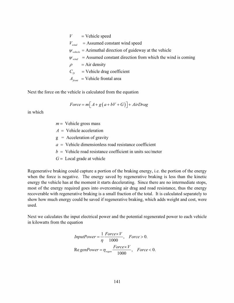
141

Vehicle speedAssumed constant wind speedAzimuthal direction of guideway at the vehicleAssumed constant direction from which the wind is comingAir densityVehicle drag coeffi

wind

vehicle

wind

D

VV

C

ψψρ

====== cient

Vehicle frontal areafrontA =

Next the force on the vehicle is calculated from the equation ( )Force m A g a bV G AirDrag= + + + +

in which

Vehicle gross mass Vehicle acceleration

g = Acceleration of gravity Vehicle dimensionless road resistance coefficient Vehicle road resistance coefficient in units sec/meter Local grade at ve

mA

abG

==

=== hicle

Regenerative braking could capture a portion of the braking energy, i.e. the portion of the energy when the force is negative. The energy saved by regenerative braking is less than the kinetic energy the vehicle has at the moment it starts decelerating. Since there are no intermediate stops, most of the energy required goes into overcoming air drag and road resistance, thus the energy recoverable with regenerative braking is a small fraction of the total. It is calculated separately to show how much energy could be saved if regenerative braking, which adds weight and cost, were used. Next we calculates the input electrical power and the potential regenerated power to each vehicle in kilowatts from the equation

1 , 0.1000

Re , 0.1000regen

Force VInputPower Force

Force VgenPower Force

η

η

×= >

×= <

142

in which η = propulsion efficiency, assumed to be 0.55 until detailed calculations with the specific

motors can be made; and regenη is the regeneration efficiency, assumed to be 0.5 until detailed calculations can improve on this number. Finally, the electrical energy used in kW-hr by all vehicles in a run is accumulated by summing the power multiplied by the computation interval dt over all vehicles and all computation intervals during a run. In equation form

,

3600ReRe .

3600

TimeIntervals Vehicles

TimeIntervals Vehicles

InputPower dtTotalElectricalEnergyUsed

genPower dtTotalPotential genPower

×=

×=

∑ ∑

∑ ∑

III. Locating and Moving Vehicles 3.1. The required number of vehicles in a network

The required number of vehicles in a PRT network is given by the formula13

peak tripop

v av

D lN

p V=

in which

peakD is the peak-period demand in people per unit of time

tripl is the average trip length

vp is the average number of people per vehicle, counting empty vehicles

avV is the average speed 3.2. Initial vehicle placement

To accomplish vehicle placement and proper identification, the station zone controller (SZC) has within it the array staVehicleInBerth(i, j), which is the number of the vehicle in berth j of station i, 0 if none. This assignment is needed so that the SZC will know where and which vehicles are in its berths, to assign incoming vehicles to the forward-most free berth, and to move vehicles forward in the station when possible.

The vehicle array Vehicle (i, j), which is stored in the computer in vehicle i, must be loaded with the correct data for each property j. Among other properties, one of them is the number of the BP ahead and the number of the BP behind vehicle i, if the BP ahead is a merge another property is the leg (0 or 1) vehicle i is on, and another gives the distance vehicle i is behind the BP ahead.

13 “Calculation of Performance and Fleet Size in Transit Systems,” JAT, 16:3(1982)231-252, equation (50).

143

This information is necessary to determine the unique arc length (s) at the vehicle, and hence from stored values of x(s), y(s), and z(s) the coordinates of the vehicle, which, in the simulation, can then be plotted. In the real system the coordinates can be compared with GPS coordinates for verification.

The domain of a zone controller is defined in terms of a range of values of arc length s. The ZC may maintain in its memory the values of x(s), y(s), and z(s) for its range of values of s. The local line speed is also maintained in memory.

3.3. Vehicle states

The vehicles can be in any one of three states: rest, constant speed, or maneuvering. If maneuvering, the command values of acceleration (A), speed (V) and position (X) from the start of the maneuver are calculated each time-multiplexing interval. In the system, position is a negative number BPD that goes to zero when the vehicle reaches the branch ahead. The reason for this measure of distance is to make the stored distance ahead of the merge the same for vehicles on the two legs of a merge that are at the same distance from the merge junction. Thus, during the maneuver

0BP BPD D X= +

where 0BPD is the negative distance at the start of the maneuver.

If a vehicle is at rest, the acceleration and speed are set to zero, and the position is given in terms of the distance BPD . If a vehicle is moving at constant speed V, distance is given by

( ) ( )BP BPD t D t t V t= −∆ + ∆

where t is time and t∆ is the time-multiplexing interval.

IV. Classification of Network Properties

To plot the position of a vehicle correctly, it is necessary to identify positively the arc length, s, ahead of the vehicle. To do this, it is necessary to identify four types of situations that relate one branch point to the branch point ahead. These types and the notation we use are the following:

brAheadTypeR(Brn) = “Right” if Brn is a merge point going to the right leg of a merge or to a diverge, or if Brn is a diverge with the right leg going to the right leg of a merge or to a diverge, as shown in the following diagram.

144

brAheadTypeR(Brn) = “Left” if Brn is a merge going to the left leg of a merge, or if Brn is a diverge with the right leg going to the left leg of a merge, as shown in the following diagram.

brAheadTypeL(Brn) = “Right” if Brn is a diverge with the left leg going either to the right leg of a merge or to a diverge, as shown in the following diagram.

brAheadTypeL(Brn) = “Left” if Brn is a diverge with the left leg going to the left leg of a merge, as shown in the following diagram.

The above arrays permit positive identification of the value of arc length, s, ahead of the vehicle. All of these quantities are calculated in the setup program.

V. Discussion of the Simulation Program

5.1. Introduction

There are two objectives to the PRT Network Simulation Program:

145

1) to develop and prove the code needed to operate a real three-dimensioal PRT network of any complexity, and

2) to provide a planning tool needed to simulate and hence design accurately any PRT system.

Both of these objectives are met with the program described here. The purpose of this section is to describe with some repition the program that will take as inputs raw data on a specific network and from it calculate and store in a set of files the information needed to run the simulation program.

A specific application is laid out first in planform, i.e., in the projection onto a horizontal plane, the x-y plain. Such a projection is defined by giving the x-y coordinates of the apexes (inter- section of tangents) to the curves, which is practical if one takes into account that curved guide- way will be at least 50% more expensive than straight guideway, so one must keep as much guideway as possible straight. To the horizontal projection we specify the height, the z-coordinates, of the apexes of vertical curves.

We use the variable s to represent uniquely every point on the network. I call s the “arc length” as it is called in analytic geometry. Thus the rectangular coordinates of a point on the guideway are designated as ( ), ( ), ( ).x s y s z s To specify the guideway to the manufacturer, we specify it as a pair of curved lines the width of the main-wheel support angles. Thus, we need also the angular coordinates, which we denote as ( ) ( ) ( ), , .azm s pitch s roll s

5.2. Apex Data In the program, apexes (intersections of the tangents to a curve) can relate to curves of any radius down to zero, i.e., no change in direction. Apexes with zero curve radius are defined at branch points where one guideway, usually the main guideway may stay straight while the other branches off in a new direction. Apexes with zero radius are also defined at points along a straight guideway where the line speed is required to change. The calculations of the coordinates of the guideway are performed in “curve-straight” sets, i.e., the curve around the apex followed by the straight segment after the apex. The program described herein calculates both the curve and the length of this straight segment, which may be of zero length. The apexes are numbered from a starting point usually but not necessarily sequentially in the direction of flow. The following data related to each apex is needed:

• The number of the next apex in the direction of flow. • At apexes at branch points, the number of the second next apex. • The x, y, and z coordinates at the apex • The intended line speed in the curve around the apex. • The intended line speed in the straight segment after the curve.

146

• The order in which the apexes are to be treated in the direction of flow. Giving this information permits branches to be added later without having to change the numbers of the previous apexs.

5.3. Station Data The stations are numbered generally but not necessarily in the direction of the flow of vehicles. The following data related to each station is needed:

• The number of the closest apex upstream of the station. • The number of the closest apex downstream of the station. • The distance of the entry diverge point into the station from the nearest upstream apex. • The side, right or left, of the main guideway the station is on. • The station type, passenger or storage. • The number of loading and unloading berths in a passenger station, or the total number of

berths in a storage station. • The separation distance between the centerline of the main line and the centerline of the

bypass line as it passes through the loading and unloading area. • The number of the branch point ahead of the station (branch point numbers are not the

same as apex numbers.) • The number of the branch point behind the station. • The number of the station ahead before the next branch point ahead, zero if none. • The number of the station behind, zero if none before the branch point behind. • The number of the nearest downstream storage station. • The station “call criterion” in terms of the number of vehicles that must be present before

an additional vehicle is called. By increasing this number, vehicles will be called sooner to reduce the wait time.

5.4. The Demand Matrix, ( , )D i j , where i is the origin station and j is the destination. The demand between a pair of stations depends on the average trip time between them. For the first calculation of the demand matrix the ridership analyst must estimate the average trip time. Runs are then made to determine the actual trip time, which is fed back into the demand model for a second iteration. Such analysis is likely to result in recommendations for changing something about the network and the station sizes. Further runs – likely a great many of them – must be performed to obtain satisfactory results. 5.5. Branch Data The branches, i.e., line-to-line merges and diverges can be numbered in any order, but usually increasing in the direction of flow. By using this notation, any network is an assembly of links, each treated the same. The following data is needed:

147

• The number of the branch point ahead, i.e., in the direction of flow. • The number of the branch point behind. • The number of the first station ahead on the same link, zero if none. • The number of the first station behind on the same link, zero if none. • The strings (“R” or “L”) brnTypeAhR(i), brnTypeAhR(i), where i is a branch point. The

meaning of these terms is given in Section IV. These terms are needed in the simulation program to determine from which side a merge is being approached.

• The switch table brnSwitch ( , )i j . It gives the direction to switch, “R” or “L”, at each diverge branch point. The switch table will be computed in a program that determines the minimum time path from any station to any other station.

5.6. Compute Azimuth All of the above information except the switch table must be picked off manually from a layout of the specific network to be simulated. To prepare to compute the curves, it is necessary first to compute the azimuth angle at each apex. The azimuth angle is taken as zero in the +x-direction, which is usually east, and is taken to increase in the counterclockwise direction. It is restrained to be less than or equal to 360 deg. 5.7. Compute Direction Change

Having the azimuth angles at all apexes, we next compute the direction change as a vehicle would move from one direction to the next. The direction change will usually be between 0 and 180 deg. 5.8. Compute Curve Properties We now have all of the information needed to compute the set-up parameters for each of the curve, which are derived in the paper “Curved Guideways.” These are the projections of the curves in the horizontal plane. In “Curved Guideways” it is shown that the vertical curves can be superimposed to get the total three-dimensional curves. 5.9. Calculate Straight Section Knowing the aX values for each curve, i.e., the distances between the apex and the start or end of the curve, which are calculated in “Curved Guideways”, we now have the information needed to calculate the length of each straight section after each curve. As mentioned, the length of the straight section may be zero, and generally is for curves that connect into a merge branch point. 5.10. Calculate Start Coordinates Next we must calculate the x-y coordinates of the point where eacht curve begins, upstream of its apex. We designate the arc length at the first point of the first curve as 0.s =

148

5.11. Calculate Station Properties The station properties that must be calculated and stored are the transition length, the length of the straight section in the station-bypass guideway, the total station guideway length, the coordinates of the starting point of the bypass guideway, and the number of berth positions counting waiting positions in each station. 5.12. Calculate Guideway Coordinates We now have all of the information needed to calculate the x-y guideway coordinates. We do so at discrete steps ,ds which we take in the first program as one meter. The end result are the coordinates ( ), ( ), ( ), ( ), ( ), ( )x s y s z s azm s pitch s roll s . To calculate these quantities we use a subroutine called Curve() to calculate the coordinates through each curve and includes superelevated turns if elected. A subroutine called Offline() calculates each offline guideway. There may be a case in which there is a change in direction of the main guideway in the region of a station, i.e., there may be an apex in the guideway in the region of a station. This requires special handling that is accomplished by a routine called SpecialOffLine(). These calculations are performed in local coordinates and then a subroutine Transform() is used to convert local coordinates into system coordinates. Subroutines GradeSetUp() and Grade() are used to add the z-coordinate and pitch angle or grade to the guideway. 5.13. Find Jump Points To position a vehicle on the guideway in the simulation program – as opposed to a real operating system – we need to know the arc length s at the vehicle, which is needed to find its space coordinates, which are needed to plot its position. In paragraph 5.12 we calculated the coordiates at discrete points ds apart. In the simulation program, the position of each vehicle is calculated at each time step as a negative distance behind the branch point ahead. This value goes positve when a vehicle passes a branch point, which indicates that it must be handed over to the next zone controller. To determine the value of arc length s at the vehicle, we must know the arc length value at the branch point ahead. To find it two steps are needed, the first is to find the coordinates and values of s at the points of arc length discontinuity, i.e., the jump points at all branch points including the station entry points. Also, there will be an additional jump point that is neither at a branch point or a station entry point, i.e., at the point 0.s = Calculation of all of these jump points is the task of this routine. 5.14 Main-guideway arc length at the Jump Points. With the coordinates of the jump points calculated, we can and must calculate the values of arc length s on the main guideway at the jump points. These values are needed to calculate the value of s at each vehicle, which as mentioned is needed to calculate the vehicle’s coordinates.

149

5.15. Find the Apex at each Branch Point corresponding to the curve there. At each branch point there are two apexs, with each corresponding to a different change in direction, often with one having no change in direction. Resolution of this difference is needed in two routines, one in calculation of the merge command point, and the other in determining the speed through the curve used in calculating the distances between branch points. In the later case, the two apexs must give the same curve speed, but in the former the largest change in direction will result in calculating the longest distance to the merge command point, which is the one required for safe merging. The apex corresponding to the greatest change in direction is thus desired and is calculated in this routine. 5.16. Calculate Distances between Branch Points and Branch Command Points This routine calculates for use in the simulation program the distance from one branch point to the branch point ahead in case of a merge, and from one branch point to the right and left branch points ahead in case of a diverge. It also records the values of arc length at the junction point on the two legs of a merge or diverge, calculates the merge command distance from each merge point, and calculates the switch command distance from each diverge point. 5.17. Calculate Negative Station Distances To the Branch Point ahead This routine calculates the following quantities;

• The negative distance from the station entry point to the branch point ahead. • The distance from the station entry point to the front of the station. • The negative distance from the front of the station to the branch point ahead. • The negative distance from the middle of the vehicle in the first berth to the branch point

ahead. • The negative distance from the command point after the station exit point to the branch

point ahead. • The negative distance from the station switch-command point to the branch point ahead. • The negative distance from the station deceleration-command point to the branch point

ahead. 5.18. LoadVehicles This routine gives each vehicle a permanently assigned number and loads it into a passenger or storage station for the start of a simulated run by giving it the following information:

• The number of the branch point ahead. • The number of the branch point behind. • The number of the station the vehicle is in.

150

• The vehicle’s switch position corresponding to the side of the main guideway the station bypass guideway is on.

• The vehicle’s destination, which now is the station it is in. • The passenger number, which is now zero. • The number of the berth the vehicle is in. • The maneuver command, which is now “None.” • The negative distance of the vehicle to the branch point ahead • The vehicle’s speed, now zero. • The vehicle’s acceleration, now zero. • The mass of the passengers aboard the vehicle, now zero. • The distance the vehicle has travelled, now zero. • The negative distance of the vehicle from the next command point, which is the

ResetOnStationExit command point.

Simultaneously, this routine gives the station-zone controller two pieces of information;

• The number of the vehicle in each berth. • The number of the vehicle in each position in the array “staVehOnStationGdwy,’ which

enables the station zone controller to keep track of each vehicle on the station off-line guideway.

5.19. Distance To the Next Station This routine determines the distance of each station to the station ahead on the same link, or to the station ahead on either branch in the nearest link or the link after that. The routine can be continued recursively until a station is found in either direction, but it will be unusual to have links with no stations. This data will be used to calculate the switch table. 5.20. The number of the next upstream station. This routine determines the number of the nearest upstream station on the same link or on the next upstream link past a merge or on either of the next upstream stations on a diverge. This data is useful for dispatcihing empty vehicles.

151

VI. Summary of Setup

1.

2.

3.

4.

Input following Apex Data for each apex, numbered in any convenient way, usually in the direction of motion, starting with 0. At each branch point there will be an apex number for each direction. Points at which there must be a speed change are given an apex number even though there may be no change in direction.

1. X coordinate 2. Y coordinate 3. Z coordinate 4. Number of next apex 5. Number of second next apex if a diverge point ahead 6. Super elevation angle in the curve around the apex 7. Speed in the curve 8. Speed in the straight segment after the curve

Layout the best initial estimate of the network on a street map. Because curved guideway is more expensive than straight guideway, use straight lines whenever possible. Locate the stations where you want them. Identify the line-to-line diverges and merges, and number them, diverges first. There must be as many diverges as merges. Establish an x-y reference frame and record the coordinates of each apex.

Input the following Station Data for each station, numbering the stations in any convenient order:

1. Number of the nearest upstream apex to the station off-line entry point. 2. Distance of the station off-line entry point to the upstream apex. 3. Designate passenger station “P”, storage station “S” 4. Number of loading and unloading berths in a passenger station, total positions in

storage station. 5. Separation between the mainline and the station by-pass or off line. 6. “L” if the station is on the left side of the main guideway while facing in the

direction of motion, “R” if the station is on the right side. 7. The number of the line-to-line diverge or merge (branch) point ahead of the station. 8. The number of the line-to-line diverge or merge (branch) point behind the station. 9. The number of the station ahead on the same link (length of guideway between

branch points), 0 if none. 10. For stations with a merge point ahead designate “L” if the station is on the left of

the merge, “R” if on the right. Designate “ ” if a diverge ahead.

Perform a graphic check of the network without showing the curves.

152

5.

6.

7.

8.

9.

10.

11.

12.

13.

Calculate the azimuth angle into each apex, assuming azimuth = 0 in the x-direction to the right. From the x-axis the azimuth angle increases in the counterclockwise direction.

Calculate the change in direction of the curve passing each apex; + counterclockwise, - clockwise.

For the curve at each apex, calculate

1. Length along the curve (arc length) of the constant jerk region of the curve. 2. The distance along the curve to the end of its constant-curvature region. 3. The local coordinates of the center of curvature of the constant-curvature region,

where the local x-axis is in the direction the curve begins, y perpendicular to the left. 4. The radius of curvature of the constant-curvature region. 5. The local end coordinates of the curve 6. The distance Xa from the curve’s apex (intersection of tangents) to the beginning of

the curve. Calculate the length of the straight segment of guideway following each curve. The straight segment may be of zero length and must be of zero length for a curve entering merge point. Every network of guideways is made up of segments consisting of a curve followed by a straight segment.

Calculate the x-y start coordinates of each curve, and from them identify the coordinates of each line-to-line branch

Calculate the x-y start coordinates of the entry off-line to each station.

Calculate and record the x-y and Azimuthal coordinates of the mainline guideway in small steps ds. This is done apex by apex for the sequence curve-straight for each apex. These calculations make use of a routine that calculates each curve in local coordinates and a second routine that transforms the local curve followed by the straight section in local coordinates into system coordinates.

Locate the main-guideway arc length at the entry point of each station. This quantity is needed to transform the local off-line-station coordinates to system coordinates.

153

14.

15.

16.

17.

18.

19.

20.

21.

22.

Locate the incremental arc length before and after each guideway jump point. The first of these will be the jump from the end of the first loop (sEnd) to the first diverge point, then to the jumps between successive branch points. These values are needed to identify the values of arc length at each merge and diverge point.

Calculate the coordinates of each off-line guideway and then transform them to system coordinates in a special way: that is in such a way that if the main line curves around an apex in the area of the off-line, the off-line guideway follows the curve.

Prepare to calculate the elevation at each point along the horizontal projection of the guideway by calculating the grade angle between each pair of apexes.

Calculate the elevation at the starting point of each curve-straight segment.

Calculate the elevation changes at each point along the horizontal projection (the x-y plane) of the guideway.

Using data from the previous routine, calculate the main-guideway arc lengths at each branch point.

Correct the merge-point arc lengths or s-values by interpolation between the segments of length ds. This is necessary at merge points because the distance to vehicles on each of the two branches of a merge must be referenced accurately to the same point.

Calculate the distance from each branch point to the next on each leg of a diverge or on the one leg of a merge.

Calculate the negative distance from the input diverge into each station to the branch point ahead.

154

23.

Requirements for ITNS Control

1. Communication must be totally secure and not subject to interference from the outside, which means that the computers cannot be connected to any external source that may be disruptive, such as the Internet. This requirement has led to the use of leaky cables within a shielded guideway, a scheme that was tested in the Raytheon test track and was first used in the Boeing AGRT program and described in publicly available papers.

2. Minimum headway. Even though early applications will not require close headways, the design of the control system must take into account the need to achieve fractional second headways safely and reliability as the system expands. Offline stations must be designed to meet expected input and output flows, and the system must be designed to prevent excessive congestion at merge points and destination stations.

3. Safety. A PRT system must provide a level of safety in terms of injuries per billion miles at least as good as a modern rapid rail system, and preferably better—better because the improvements provided by PRT in all areas must be good enough to justify the development cost. To achieve this level of safety, the on-board and wayside computers must be dual duplex. Safety must not depend on one set of computers, i.e., vehicle flow must be monitored by wayside zone-control computers, which requires wayside measurement of position and speed.

4. Ride Comfort. Longitudinal maneuvers must be performed in such a way that International Standards Organization ride comfort standards on acceleration as a function of frequency are met. In maneuvers, longitudinal acceleration must be limited to 0.25 g, lateral acceleration to 0.2 g and jerk to 0.25 g/s in normal operation. The maximum emergency-braking deceleration depends on whether or not passenger constraints are provided. If not, the requirement must be that the passenger must not slide off the seat in an emergency stop. With passenger constraints, twice the normal values are permitted. The control system must not be a factor in causing motion sickness.

5. Changing Conditions. The control system must be able to reduce cruising speed in high winds, restore speed smoothly when the wind dies down, and must be able to cope with any unusual

Calculate the positions of the following command points:

1. Station switch command point. 2. Station deceleration command point. 3. Merge command point. 4. Diverge command point

155

situation, such as a stopped vehicle, that would require vehicles to slow down or stop away from a station.

6. Dead-Vehicle Detection. It must be possible to detect a dead vehicle on the guideway, however remote that possibility may be. Each vehicle must transmit its speed and position at frequent intervals to a wayside computer—a zone controller. If the zone controller suddenly does not receive the expected signal, it must be programmed to remove the speed signal for all vehicles in that link and transmit this information to the next upstream zone controller. Each vehicle's control system must be configured to command reduction in speed to a creep speed if the zone controller's speed signal is not received. A finite creep speed permits vehicles ahead of the failed vehicle to move safely to the next zone, it reduces anxiety, and with seated passengers is safe. Magnetic detectors must be placed at specified intervals along the guideway to inform the zone controller of passage of a vehicle independent of the vehicle controller. Thus, if a vehicle passes one of these markers and not the next, the location of the dead vehicle is approximately known. Then, because the passengers are seated and can be protected, and the vehicle will be protected by appropriately designed shock-absorbing bumpers, a creeping vehicle can be permitted to advance until it soft engages with the dead vehicle, whereupon the position of the dead vehicle becomes known and the failure strategy can be engaged.

7. Interchange Flexibility. The simplest interchange is a Y. Such an interchange gives the least visual impact at any one point, but requires that vehicles first merge, then diverge, which creates a bottleneck after merging. To obtain maximum possible throughput, two-in, two-out, multilevel interchanges can be used. They permit vehicles to diverge first and then merge. With such interchanges, the input and output capacity of the lines is the same, hence the worst that can happen is that a vehicle may have to be diverted from the direction it would normally go. Thus the control system does not have to be concerned with sending too much traffic along a particular line. If Y-interchanges are used, control actions are not limited to one interchange; however, they are often necessary. Thus, the control system must permit them.

8. Vandalism and Sabotage. A system in which the control functions are distributed and the wayside computers are protected, for example in safe rooms under the stations, will be less susceptible to malicious damage than a system in which a central computer plays an essential role. To minimize the consequences of failures of any kind, distributed control is preferred. The required central-computer functions should be such that the worst that can happen if it fails is that the system will operate less efficiently.

9. Modularity. The control units must be easily exchangeable so that down time is minimized.

10. Expandability. The control system must be designed for easy system expansion.

156

Distance to Slip

Velocity-Time Diagram, Mirror Symmetry about point 3.

The purpose of this paper is to determine the distance required for a vehicle to slip one or more headway lengths. To do this I make use of the above velocity-time diagram of two slip maneuvers. The jerk from point 0 to point 1 is –Jc, from point 1 to point 2 is zero, and from point 2 to point 3 is +Jc in which Jc is the magnitude of the maximum comfort jerk. I assume the reader is familiar with the three equations for the transition from one point to the next at constant jerk, viz.:

1) The time interval between two points at constant jerk is the quantity new acceleration minus old acceleration divided by jerk, or if jerk is zero, the quantity new speed minus old speed divided by acceleration.

2) The new speed is the old speed plus the time interval multiplied by the average acceleration.

3) The distance interval is the time interval multiplied by the quantity old speed plus the time interval multiplied by the quantity twice old acceleration plus new acceleration divided by six.

157

Equations for the general case.

The time, speed, and distance relationships during the interval from point 0 to point 1 are

1 1 101 1 01 01 01 01 1, , , 0

2 6L Lc

A A Adt V V dt dx dt V dt AJ

= = + = + < − (1)

In which A1 is the negative acceleration at point 1, VL is the line speed, V1 is the speed at point 1, dt01 is the time interval from point 0 to point 1, and dx01 is the distance travelled in moving from point 0 to point 1.

The similar relationships in going from point 1 to point 2 at constant deceleration are

( )2 21 22 1 1

12 2 1 12 1 12 12 1 12 11 1

, , , 02 2

V VV V Adt V V dt A dx dt V dt AA A

−− = = + = + = < − (2)

In going from point 2 to point 3 we have

1 1 1 123 01 3 2 23 23 23 2 23 23 3 01, ,

2 3 6c

A A A Adt dt V V dt dx dt V dt dt V dtJ− = = = + = + = −

(3)

The usual case A1 = -Ac

If A1 = -Ac, where Ac is the maximum comfort value of acceleration, we have

( )

2 2

01 1 01

2 333 31 2 1 2

12 12

2 2

23 01 3 2 23 3

, ,2 6

,2 2

, ,2 6

c c c cL L

c c c c

LL c L c

c c c c c c

c c c

c c c

A A A Adt V V dx VJ J J J

V VV V A V V AV V V Vdt dxA A J A A J

A A Adt dt V V dx VJ J J

= = − = −

+ − −− −

= = − = = −

= = − = +

(4)

( )

303 01 12 23

3 303 01 12 23

303

22

2

L c

c c

L c L c

c c c

L

V V Adt dt dt dtA J

V V A V V Adx dx dx dxJ A J

V V dt

−= + + = +

+ −= + + = + −

+ =

(5)

Let S = Slip, Tm = 2dt03 = maneuver time, and Dm = 2dx03 = maneuver distance. Then

158

( )

( )

( )

( )

33

3 33

22

2

3 2

2 2

, let

4 /Then 0, 1 12 /

4 /1 12 /

L mL m m m L L

L c LL

c c c

c c c

c c c c c

c cL

c c c

V V TS V T D T V V V

V V A V VV V xA J A

A A S ASx x xJ A J A J

A S AV VJ A J

+ = − = − = − − −

= − + =

+ − = = + −

= − + −

(6)

The smallest value of S for which equations (6) apply occurs when V2 = V1. Then, from equations (4),

3L c

c c

V V AA J−

=

Then, from the second line of equations (6)

2

min 1 2 cc

c

AS S S AJ

= = =

(7)

We usually assume Ac = 0.25g, Jc = 0.25 g/s. Then Smin = 4.9 m and VL – V3 = 0.25g = 2.45 m/s. The distance travelled in the headway time Th is VLTh. We want to consider slipping one headway distance. Then, if we set VLTh = Smin the corresponding speed is VL = 4.9m/Th.

Case for small S.

For small headways, we will have cases in which S < Smin. In such cases set dt12 = 0 in equations (1) and (3) to get

( )

2 21 1 1

01 1 01 01 1

2 2 21 1 1 1

23 3 1 23 01 1 01

21 1 1

1/33 21

12

, , , 02 6

5, ,2 3 6

4 , 2 2

2 ,2

L Lc c c

Lc c c c

m m Lc c c

cL m m

c

A A Adt V V dx dt V AJ J J

A A A Adt V V dx dt V dt VJ J J J

A A AT D VJ J J

A J SS V T D AJ

= = − = − < −

−= = − = − = −

= − = − −

− = − = = −

(8)

159

Case for Large S.

We will need to set a minimum speed V3 = Vmin, which will be reached for large values of slip. In this case

( ) min2 min

cLL

c c

AV VS S V VA J

−= = − +

(9)

If S > S2 we must add a section of time dt34 between the descending and ascending speed regions, in which

234

min

.S SdtV−

= (10)

Setup Code

The given parameters are

min, , ,c c LA J V V

Then calculate

( )2

min1 2 min2 ,c cL

c Lc c c

A AV VS A S V VJ A J

−= = − +

.

Given S then

If 1S S≤ then

1/32 2

11 1 3 1

1/3

101 12 23 01 34 45 01 56 67 01

21 1 1

01 01 01 12 23 01 1 01 01

, , ,2 2

, 0, , 0, , 0,2

5, 0,6 3 6

cL

c

c c

L Lc

J S AA dV V V dV V V dVJ

A Sdt dt dt dt dt dt dt dt dt dtJ J

A A Adx dt V dt dx dx dt V dt dt VJ

= − = = − = −

= − = = = = = = =

= + = = + = −

( )

34

45 23 56 67 01

1/3 2 /31/ 221

01 23 01

, 0

, 0,

42 2 2 22

cm L L

c c

dx

dx dx dx dx dx

J SA SD dx dx dt V VJ J

=

= = =

= + = − = −

160

else

If 2S S≤ then

( )

2

3 34 3424 /1 1 , 0, 0

2 /c c

Lc c c

A S AV V dt dxJ A J

= − + − = =

else

( ) ( )3 min 34 2 min 34 min 34, / , .LV V dt S S V V dx V dt= = − − =

end if

( )

( ) ( )

( )

01 1 01 01 01 01

23 01 2 3 23 23 23 2 23 01 3 01

2 21 2 1 2

12 12 12 1 12

45 23 56 12 67 01

45 23 56 12

, / 2, / 6

, / 2, / 3 / 6

, / 22

, ,, ,

cL c L c

c

c c c

cc c

Adt V V dt A dx dt V dt AJ

dt dt V V dt A dx dt V dt A dt V dt A

V V V Vdt dx dt V dt AA A

dt dt dt dt dt dtdx dx dx dx d

= = − = −

= = + = − = +

− −= = − =

= = == =

( ) ( ) ( )( ) ( )

( )

67 01

3 303 01 01

2 203 01 3 01 3 3 01

3 3301 03

33 2

2

12

2 2

, if 0 else 0.

L L c

c c c

L L L c cc

L LL

c

L c mm L

c c L m

x dxV V V V Adt dt dt

A A J

dx dt V V V V dt A V V dt AA

V V V VV Vdt dtA

V V A VD V V S S e e eA J V V

=− −

= + − = +

= + + − − +

+ + −= + =

−

= + + + − = > −

end if

1 01 1 01

2 1 12 2 1 12

3 2 23 3 2 23

4 3 34 4 3 34

5 4 45 5 4 45

6 5 56 6 5 56

7 6 67 7 6 67

t dt x dxt t dt x x dxt t dt x x dxt t dt x x dxt t dt x x dxt t dt x x dxt t dt x x dx

= == + = += + = += + = += + = += + = += + = +

161

The run code is now

Initial conditions: 0, 0, , 0Lt x V V A= = = =

1

2

3

4

5

6

7

0

0

0

0

c

c

c

c

if t tJerk J

elseif t tJerk

elseif t tJerk J

elseif t tJerk

elseif t tJerk J

elseif t tJerk

elseif t tJerk J

elseJerk

endif

<= −<=<=<=<=<=<= −

=

2 3

22 6

2

dt dtx x Vdt A Jerk

dtV V Adt Jerk

A A Jerk dtt t dt

= + + ⋅ + ⋅

= + + ⋅

= + ⋅= +

Distance Merge Point to Clearance Point, Dm-S

Slip V3 V3,used Dm,base Dm Dm-Sprev

m m/s m/s m m m

g= 9.807 m/s^2 1 5.0 7.516 7.516 35.262 35.262 35.262

Ac= 2.452 m/s^2 2 10.0 6.125 6.125 41.612 41.612 36.612

Jc= 2.452 m/s^3 3 15.0 5.039 5.039 45.471 45.471 35.471

162

tJ= 1 s 4 20.0 4.117 4.500 47.029 48.797 33.797

VL= 10 m/s 5 25.0 3.302 4.500 47.029 52.888 32.888

Th= 0.5 s 6 30.0 2.563 4.500 47.029 56.979 31.979

Vmin= 4.500 m/s 7 35.0 1.882 4.500 47.029 61.070 31.070

S1= 4.903 m 8 40.0 1.247 4.500 47.029 65.161 30.161

S2= 17.839 m 9 45.0 0.651 4.500 47.029 69.252 29.252

10 50.0 0.086 4.500 47.029 73.343 28.343

11 55.0 -0.451 4.500 47.029 77.434 27.434

12 60.0 -0.964 4.500 47.029 81.525 26.525

13 65.0 -1.457 4.500 47.029 85.616 25.616

14 70.0 -1.932 4.500 47.029 89.706 24.706

15 75.0 -2.390 4.500 47.029 93.797 23.797

Conclusion

The maximum maneuver distance for a slip maneuver beyond the merge command point is produced by the vehicle one headway interval behind the merge command point. This distance is

( )

( )

2

3 2

3 min 3 min

33 2

4 /1 1 where 22 /

if then

Minimum Merge Length Clearance Length

c cL L h

c c c

L c mm L

c c L m

m L h

A S AV V S V TJ A J

V V V V

V V A VD V V S SA J V V

D V T

= − + − =

< =

−= + + + − −

= − +

Computer Program

'This routine SLIPHDWY.BAS calculates maneuvers for slipping N headway distances. 'Units are MKS g = 9.80665 Ac = .25 * g Jc = .25 * g tJ = Ac / Jc VL = 9 Vmin = .4 * VL Th = .5 'minimum headway S1 = 2 * Ac * tJ ^ 2

163

dV = VL - Vmin S2 = dV * (dV / Ac + tJ) dt = .0002 'computation interval SCREEN 9 COLOR 7, 8 T0 = 10 Y0 = 250 ScaleT = 15 ScaleX = 2 ScaleV = 10 ScaleA = 10 LINE (T0, Y0)-(640, Y0) LINE (T0, Y0)-(T0, 0) LINE (T0, Y0 - ScaleV * VL)-(640, Y0 - ScaleV * VL) PRINT " i S Dm Dm - S Dm / S" FOR i = 1 TO 20 'Initial conditions t = 0 x = 0 V = VL A = 0 S = VL * Th * i IF S <= S1 THEN A1 = -(Jc ^ 2 * S / 2) ^ (1 / 3) dV = .5 * A1 ^ 2 / Jc V1 = VL - dV V3 = V1 - dV dt01 = -A1 / Jc dt12 = 0 dt23 = dt01 dt34 = 0 dt45 = dt23 dt56 = 0 dt67 = dt01 dx01 = dt01 * (VL + dt01 * A1 / 6) dx12 = 0 dx23 = dt23 * (V1 + dt23 * A1 / 3) dx34 = 0 dx45 = dx23 dx56 = 0 dx67 = dx01 ELSE IF S <= S2 THEN V3 = VL - .5 * tJ * Ac * (SQR(1 + (4 * S / Ac) / tJ ^ 2) - 1) dt34 = 0 dx34 = 0 ELSE V3 = Vmin dx34 = S - S2 dt34 = dx34 / Vmin END IF dt01 = tJ V1 = VL - dt01 * Ac / 2

164

dx01 = dt01 * (VL - dt01 * Ac / 6) dt23 = dt01 V2 = V3 + dt23 * Ac / 2 dx23 = dt23 * (V2 - dt23 * Ac / 3) dt12 = (V1 - V2) / Ac dx12 = dt12 * (V1 - dt12 * Ac / 2) dt45 = dt23 dt56 = dt12 dt67 = dt01 dx45 = dx23 dx56 = dx12 dx67 = dx01 END IF Tm = 2 * (dt10 + dt12 + dt23) + dt34 Dm = 2 * (dx01 + dx12 + dx23) + dx34 t1 = dt01 t2 = t1 + dt12 t3 = t2 + dt23 t4 = t3 + dt34 t5 = t4 + dt45 t6 = t5 + dt56 t7 = t6 + dt67 x1 = dx01 x2 = x1 + dx12 x3 = x2 + dx23 x4 = x3 + dx34 x5 = x4 + dx45 x6 = x5 + dx56 x7 = x6 + dx67 DO IF t < t1 THEN Jerk = -Jc ELSEIF t < t2 THEN Jerk = 0 ELSEIF t < t3 THEN Jerk = Jc ELSEIF t < t4 THEN Jerk = 0 ELSEIF t < t5 THEN Jerk = Jc ELSEIF t < t6 THEN Jerk = 0 ELSEIF t < t7 THEN Jerk = -Jc ELSE Jerk = 0 END IF x = x + V * dt + A * dt ^ 2 / 2 + Jerk * dt ^ 3 / 6 V = V + A * dt + Jerk * dt ^ 2 / 2 A = A + Jerk * dt

165

t = t + dt PSET (T0 + ScaleT * t, Y0 - ScaleX * x), 10 PSET (T0 + ScaleT * t, Y0 - ScaleV * V), 11 PSET (T0 + ScaleT * t, Y0 - ScaleA * A), 12 PSET (T0 + ScaleT * t, Y0 - ScaleA * Jerk), 13 LOOP UNTIL t > t7 + 1 PRINT i; PRINT USING "####.###"; S; Dm; Dm - S; Dm / S NEXT i Potential Headway Violation upon Decelerating into a Station

Figure 1. The velocity profiles of a pair of vehicles entering a station.

Consider a vehicle #1 decelerating into a station to station speed staV , followed by a vehicle #2 a time Line Headway behind undergoing the same maneuver. Let the position of vehicle #1 at time zero be (0) 0.x = The times, accelerations, speeds, and positions of vehicle #1 at the points 1, 2, 3 in Figure 114 are as follows:

14 For the methodology, see the internal paper “Speed and Position vs. Time”

V

t

0 1 2 3

Line Headway

VL

1

2

Vstation

166

01 1 01 01 01 01

23 2 23 23 23 2 23

1 212 12 12 1 12

1 01 2 1 12 3 2 23

1 01 2 1 12 3 2 23

, ,2 6

, ,2 3

,2

, ,, ,

c c cL L

c

c c csta

c

c

c

A A Adt V V dt dx dt V dtJA A Adt V V dt dx dt V dtJ

AV Vdt dx dt V dtA

t dt t t dt t t dtx dx x x dx x x dx

= = − = −

= = + = −

− = = −

= = + = += = + = +

(1)

From equations (1) we find

2 2

03 01 23 1212

2 2c c c L sta c

L stac c c c c c

A A A V V Adt dt dt dt V VJ A J J A J

−= + + = + − − − = +

(2)

Thus, the maneuver time from line speed to station speed is

L sta cm

c c

V V ATA J−

= + (3)

From equations (1) we also find

( )

( ) ( )( ) ( ) ( )

( ) ( )

2 2 21 2

03 01 23 12 1 2

2

1 2 1 2

03

2 6 3 2

1 12 2

2 2

c c c cL sta

c c c c c

c c cL sta L sta L sta L sta

c c c c c

L sta L staL sta c

c c

A A A A V Vdx dx dx dx V V V VJ J J J A

A A AV V V V V V V V V V V VJ A J A J

V V V VV V A dtA J

−= + + = + + − − + +

= + + − + = + + − − +

+ + −= + =

(4)

Thus, the distance traveled from line speed to station speed is

( )

2L sta

m m

V VD T

+= (5)

167

Using the above canonical formulation, the acceleration, speed, and position of vehicle 1 at any value of t are as follows:

( )

1

1 2 1 1 1 1

2 3 2 2 2 2

0 : , , ,2 6

: , , ,2

: , , ,2 3

c L L

c

cc c

A At t t t A J t V V t x t V t

At t t t t t A A V V tA x x t V t

A A At t t t t t A A J t V V t x x t V t

≤ ≤ ∆ = = − ∆ = + ∆ = ∆ + ∆

≤ ≤ ∆ = − = − = + ∆ = + ∆ + ∆

− + ≤ ≤ ∆ = − = − + ∆ = + ∆ = + ∆ + ∆

(6)

For vehicle #2 up to time t LineHeadway= the speed stays constant at LV and the distance traveled is

Lx V t= . For t LineHeadway> we can obtain the acceleration, speed, and position as functions of time by making the following substitutions in equations (5): t t LineHeadway→ −

( )

1

1 2 1 1 1 1

0 : 0, ,

: , , ,2 6

: , , ,2

h

h L L h

h h h c L L

h h c

T LineHeadwayt T A V V x V t T

A AT t t T t t T A J t V V t x t V t

AT t t T t t t t A A V V tA x x t V t

=

≤ ≤ = = = −

≤ ≤ + ∆ = − = − ∆ = + ∆ = ∆ + ∆

+ ≤ ≤ + ∆ = − = − = + ∆ = + ∆ + ∆

( )2 3 2 2 2 2: , , ,

2 3c

h h c c

A A AT t t T t t t t A A J t V V t x x t V t− + + ≤ ≤ + ∆ = − = − + ∆ = + ∆ = + ∆ + ∆

(7)

The Minimum Headway

Figure 2. A pair of vehicles moving to the right.

#1 #2

D1

L D2

Hmin

V1 V2

168

Assume vehicle #1 stops due to a failure at deceleration fA and jerk .fJ From equation (5), the stopping distance of vehicle #1 is

1 11 2

f

f f

AV VDA J

= +

(8)

After a control time delay ,ct vehicle #2 stops at the emergency deceleration rate eA and

emergency jerk .eJ Its stopping distance is therefore

2 22 2 2

ec

e e

AV VD V tA J

= + +

(9)

Assuming the length of each of the two vehicles is L , the minimum allowable separation between them is

min 2 1H L D D= + − (10)

The minimum permissible time headway is therefore

min

2

HMinHeadwayV

=

(11)

A program to calculate the acceleration, speed, positions profiles and the minimum headway is given in the Appendix. Some results are given in Figures 3 and 4.

0 1 2 3 4

TIME, seconds

-10

0

10

20

30

40

Acce

lerati

on, s

peed

, and

dista

nce t

rave

lled i

n MKS

units Acceleration of veh 1

Speed of veh 1Distance veh 1 has traveledAcceleration of veh 2Speed of veh 2Distance veh2 has traveled

169

Figure 3. Kinematics of motion of a pair of vehicles decelerating to station speed.

Figure 4. Separation and minimum allowable separation between two vehicles entering a station.

The parameters used in Figures 3 and 4 are those given at the beginning of the program shown in the Appendix. Many runs can be made for different accelerations and jerks. For the set shown in the program, runs were made with different line headways and control time constants to obtain the maximum negative separations as shown in Table 1 and as calculated by the program.

Table 1. Maximum headway violations for the cases shown.

\ct LineHeadway → 0.5 1.0 1.3 1.5

0.05 -3.25 -1.03 0 0 0.10 -3.80 -1.59 -0.03 0 0.15 -4.36 -2.15 -0.60 0 0.20 -4.92 -2.71 -1.17 -0.01

It is seen that if the line headway between two vehicles sequentially entering a station is to be as low as one second, the control time constant must be quite small, but not particularly small using contemporary technology. Note from Figure 4 that in the case shown the small headway violation increases from zero back to zero in about one second.

In this work, we considered only the portion of the maneuver from line speed to station speed. Further development of the program included in the Appendix shows that, since the second of the pair of vehicles will be stopping at least one berth behind the first, there is no headway violation in the maneuvers from station speed to rest.

0 1 2 3 4

TIME, seconds

0

1

2

3

4

5

6

7

8

9

10

11

12

13

Actua

l and

mini

mum

sepa

ratio

ns, m

eters

Separation between veh 1 and 2Minimum allowable separation

170

Appendix 'This program MINHEAD.BAS calculates the minimum headway permissible 'between a pair of vehicles decelerating into a station 'Units are MKS DEFDBL A-Z DIM Counter AS INTEGER DIM A(1 TO 2) AS DOUBLE 'acceleration of vehicles 1 & 2 DIM V(1 TO 2) AS DOUBLE 'speed of vehicles 1 & 2 DIM X(1 TO 2) AS DOUBLE 'position of vehicles 1 & 2 DIM t4(1 TO 2) AS DOUBLE 'time at end of station-speed section DIM t5(1 TO 2) AS DOUBLE 'time at command to constant deceleration DIM t6(1 TO 2) AS DOUBLE 'time at command to constant jerk DIM t7(1 TO 2) AS DOUBLE 'time at maneuver end, total maneuver time DIM X1(1 TO 2) AS DOUBLE 'position of command to constant deceleration DIM X2(1 TO 2) AS DOUBLE 'position of command to constant jerk DIM X3(1 TO 2) AS DOUBLE 'position at beginning of station-speed section DIM X4(1 TO 2) AS DOUBLE 'position at end of station-speed section DIM X5(1 TO 2) AS DOUBLE 'position of command to constant deceleration DIM X6(1 TO 2) AS DOUBLE 'position of command to constant jerk DIM X7(1 TO 2) AS DOUBLE 'position at maneuver end, total maneuver distance DIM D(1 TO 2) AS DOUBLE 'stopping distances of vehicles 1 & 2 g = 9.80665 'acceleration of gravity Ac = .25 * g 'comfort deceleration Jc = .25 * g 'comfort jerk tJ = Ac / Jc 'jerk time constant Af = .4 * g 'maximum failure deceleration Jf = .4 * g 'maximum failure jerk Ae = .4 * g 'emergency deceleration Je = .8 * g 'emergency jerk VL = 12 'line speed Vsta = 8 'station speed tc = .15 'time constant Lveh = 2.743 'vehicle length B = 3.048 'berth length LineHeadway = .5 'time headway between vehicles while at line speed t = 0 'start time dt = .01 'computational time interval 'Calculation of the maneuver increments and transition speeds dt01 = tJ V1 = VL - dt01 * Ac / 2 dx01 = dt01 * (VL - Ac * dt01 / 6) dt23 = tJ V2 = Vsta + dt23 * Ac / 2 dx23 = dt23 * (V2 - dt23 * Ac / 3) dt12 = (V1 - V2) / Ac dx12 = dt12 * (V1 - dt12 * Ac / 2) dx34 = 10 'distance vehicle 1 travels at station speed dt34 = dx34 / Vsta 'time of veh 1 at station speed

171

dt45 = tJ V5 = Vsta - dt45 * Ac / 2 dx45 = dt45 * (Vsta - dt45 * Ac / 6) dt67 = tJ V6 = dt67 * Ac / 2 dx67 = dt67 * (V6 - dt67 * Ac / 3) dt56 = (V5 - V6) / Ac dx56 = dt56 * (V5 - dt56 * Ac / 2) 'Times and position increments at the transition points t1 = dt01 t2 = t1 + dt12 t3 = t2 + dt23 t4(1) = t3 + dt34 'this and following times for veh 1 t5(1) = t4(1) + dt45 t6(1) = t5(1) + dt56 t7(1) = t6(1) + dt67 'maneuver time t4(2) = t3 + dt34 - B / Vsta 'this and following times for veh 2 t5(2) = t4(2) + dt45 t6(2) = t5(2) + dt56 t7(2) = t6(2) + dt67 'maneuver time X1(1) = dx01 X2(1) = X1(1) + dx12 X3(1) = X2(1) + dx23 X4(1) = X3(1) + dx34 X5(1) = X4(1) + dx45 X6(1) = X5(1) + dx56 X7(1) = X6(1) + dx67 X1(2) = dx01 X2(2) = X1(2) + dx12 X3(2) = X2(2) + dx23 X4(2) = X3(2) + dx34 - B 'veh 2 stops one berth short of veh 1 X5(2) = X4(2) + dx45 X6(2) = X5(2) + dx56 X7(1) = X6(1) + dx67 'total maneuver distance CLS SCREEN 9 COLOR 7, 8 scaleT = 600 / t7(2) scaleA = 10 scaleV = 10 scaleX = 4 scaleS = 40 T0 = 10 Y0 = 280 LINE (T0, Y0)-(640, Y0) LINE (T0, Y0)-(T0, 0) OPEN "KINEMAT.ASC" FOR OUTPUT AS #1 OPEN "SEPRATN.ASC" FOR OUTPUT AS #2 DO 'Motion of first vehicle

172

IF t <= t1 THEN DelT = t A(1) = -Jc * DelT V(1) = VL + DelT * A(1) / 2 X(1) = DelT * (VL + DelT * A(1) / 6) ELSEIF t <= t2 THEN DelT = t - t1 A(1) = -Ac V(1) = V1 + DelT * A(1) X(1) = X1(1) + DelT * (V1 + DelT * A(1) / 2) ELSEIF t <= t3 THEN DelT = t - t2 A(1) = -Ac + Jc * DelT V(1) = V2 + DelT * (-Ac + A(1)) / 2 X(1) = X2(1) + DelT * (V2 + DelT * (-2 * Ac + A(1)) / 6) ELSEIF t <= t4(1) THEN DelT = t - t3 A(1) = 0 V(1) = Vsta X(1) = X3(1) + Vsta * DelT ELSEIF t <= t5(1) THEN DelT = t - t4(1) A(1) = -Jc * DelT V(1) = Vsta + DelT * A(1) / 2 X(1) = X4(1) + DelT * (Vsta + DelT * A(1) / 6) ELSEIF t <= t6(1) THEN DelT = t - t5(1) A(1) = -Ac V(1) = V5 + DelT * A(1) X(1) = X5(1) + DelT * (V5 + DelT * A(1) / 2) ELSEIF t < t7(1) THEN DelT = t - t6(1) A(1) = -Ac + Jc * DelT V(1) = V6 + DelT * (-Ac + A(1)) / 2 X(1) = X6(1) + DelT * (V6 + DelT * (-2 * Ac + A(1)) / 6) ELSE A(1) = 0 V(1) = 0 X(1) = X7(1) END IF 'Motion of second vehicle tsec = t - LineHeadway IF tsec <= 0 THEN DelT = tsec A(2) = 0 V(2) = VL X(2) = DelT * VL ELSEIF tsec <= t1 THEN DelT = tsec A(2) = -Jc * DelT V(2) = VL + DelT * A(2) / 2 X(2) = DelT * (VL + DelT * A(2) / 6) ELSEIF tsec <= t2 THEN DelT = tsec - t1 A(2) = -Ac V(2) = V1 + DelT * A(2)

173

X(2) = X1(2) + DelT * (V1 + DelT * A(2) / 2) ELSEIF tsec <= t3 THEN DelT = tsec - t2 A(2) = -Ac + DelT * Jc V(2) = V2 + DelT * (-Ac + A(2)) / 2 X(2) = X2(2) + DelT * (V2 + DelT * (-2 * Ac + A(2)) / 6) ELSEIF tsec <= t4(2) THEN DelT = tsec - t3 A(2) = 0 V(2) = Vsta X(2) = X3(2) + Vsta * DelT ELSEIF tsec <= t5(2) THEN DelT = tsec - t4(2) A(2) = -Jc * DelT V(2) = Vsta + DelT * A(2) / 2 X(2) = X4(2) + DelT * (Vsta + DelT * A(2) / 6) ELSEIF tsec <= t6(2) THEN DelT = tsec - t5(2) A(2) = -Ac V(2) = V5 + DelT * A(2) X(2) = X5(2) + DelT * (V5 + DelT * A(2) / 2) ELSEIF tsec < t7(2) THEN DelT = tsec - t6(2) A(2) = -Ac + Jc * DelT V(2) = V6 + DelT * (-Ac + A(1)) / 2 X(2) = X6(2) + DelT * (V6 + DelT * (-2 * Ac + A(1)) / 6) ELSE A(2) = 0 V(2) = 0 X(2) = X7(2) END IF D(1) = .5 * V(1) * (V(1) / Af + Af / Jf) 'stopping distance of veh #1 D(2) = .5 * V(2) * (V(2) / Ae + Ae / Je) 'stopping distance of veh #2 Separation = X(1) - X(2) IF Separation < Lveh + V(2) * tc THEN SLEEP IF V(2) > 0 THEN Headway = Separation / V(2) MinSeparation = Lveh + V(2) * tc + D(2) - D(1) IF V(2) > 0 THEN MinHeadway = MinSeparation / V(2) dSep = Separation - MinSeparation IF dSep < MaxNegSep THEN MaxNegSep = dSep PSET (T0 + scaleT * t, Y0 - scaleA * A(1)), 14 PSET (T0 + scaleT * t, Y0 - scaleV * V(1)), 13 PSET (T0 + scaleT * t, Y0 - scaleX * X(1)), 12 PSET (T0 + scaleT * t, Y0 - scaleA * A(2)), 11 PSET (T0 + scaleT * t, Y0 - scaleV * V(2)), 10 PSET (T0 + scaleT * t, Y0 - scaleX * X(2)), 9 PSET (T0 + scaleT * t, Y0 - scaleS * Separation), 5 PSET (T0 + scaleT * t, Y0 - scaleS * MinSeparation), 6 'PRINT USING "#####.##"; t; A(1); V(1); X(1) ; A(2); V(2); X(2); Separation; MinSeparation 'PRINT USING "#####.##"; t; V(2); Separation; Separation - Lveh - V(2) * tc; MinSeparation; dSep; Headway; MinHeadway

174

IF Counter = 20 THEN Counter = 0 'SLEEP END IF Counter = Counter + 1 'WRITE #1, t, A(1), V(1), X(1), A(2), V(2), X(2) 'WRITE #2, t, Separation, MinSeparation t = t + dt LOOP UNTIL t > t7(2) + 1 PRINT " MaxNegSep = "; PRINT USING "###.##"; MaxNegSep CLOSE #1 CLOSE #2

Some History of PRT Simulation Programs J. Edward Anderson, Ph.D., P. E.

Abstract

This paper documents 32 vehicle simulation programs that have been developed since 1969 to simulate the operation of automated vehicles operating in networks of guideway under a variety of strategies.

Introduction

Every group intent on designing a marketable Personal Rapid Transit system has needed to have close at hand a simulation program that permits detailed study of the system’s performance characteristics both for design and planning purposes. Since all or any assumptions made in developing the simulation must be thoroughly understood; each group, practically speaking, must develop its own simulation program. Many engineers have understood this necessity and in time I expect that the details will be taught in engineering courses to the benefit of not only PRT designers, but the consulting firms and planners who need to know the details. Over the 40 years in which I have been involved in PRT research, development and design I have become aware of 32 automated vehicle simulation programs of varying degrees of completeness, and it is my purpose in writing this paper to call attention to and discuss them, with the hope thereby that the best ideas will come into common use as the field of PRT matures. The simulation tool is the slide rule of PRT development. If there are additional similar simulation programs, I regret not including them, but I simply am not aware of them.

1970s Era PRT Network Simulation Programs

During the 1970s, at least the following organizations or individuals developed PRT simulation programs:

1. Royal Aircraft Establishment, Ministry of Defense, Farnborough, UK 2. The Aerospace Corporation, El Segundo, CA 3. Morgantown PRT Program

175

4. Morse Wade, IBM Corporation, Poughkeepsie, NY 5. Applied Physics Laboratory, Johns Hopkins University 6. Prof. Harold York, University of Minnesota 7. Marvin A. Sirbu, Massachusetts Institute of Technology 8. IBM Corporation, Gaithersburg, MD 9. Kandasamy Thangavelu, Colorado Regional Transportation District 10. Johnson, Walter & Wilde, Colorado Regional Transportation District 11. S & A Systems, Dallas, Texas 12. Dr. Sakasita, Colorado Regional Transportation District 13. Professor Alain Kornhauser, Princeton University 14. Messerschmitt-Bölkow-Blohm, Munich 15. University of Karlsruhe, West Germany 16. Raytheon Missile Systems Division

Royal Aircraft Establishment

D. I. Paddison, “Cabtrack Studies: Estimation of Capacity of Cabstops,” RAE Technical Report 71132, June 1971. 49 pages and 10 figures. J. C. H. Longrigg, “Cabtrack Studies: Data Sheets for Track Layouts,” RAE Technical Report 71024, February 1971. 32 pages and 7 figures. The Summary of Paddison’s report contains the statement: “Results are presented of a digital computer simulation of the operation of six small and medium-sized Cab-stops.” We now refer to “Cab-stops” as “Stations.” Section 1.2 of Paddison’s report contains the sentence: “Study of the control of a complete network will require a simulation of a network in operation.” None of the RAE reports I have seen discuss a complete network simulation, but I have not seen all of the reports the study produced. However, Longrigg provides the formulae needed for calculating all of the curves and off-line transitions used in a complete PRT network.

The Aerospace Corporation

A. V. Munson, Jr., H. Bernstein, J. R. Buyan, K. J. Liopiros, and T. E. Travis of The Aerospace Corporation, “Quasi-Synchronous Control of High-Capacity PRT Networks,” PRT15, pp. 325-350. On page 349 the following paragraphs can be found:

B. “The PRT network simulation was implemented to assist in establishing system performance parameters such as trip times, waiting times, empty car trip lengths, and guideway and stations loadings as a function of system configuration and operating strategies. A

15 J. E. Anderson, J. L. Dais, W. L. Garrard, A. L. Kornhauser, Personal Rapid Transit, Institute of Technology, University of Minnesota, April 1972.

176

secondary but quite important objective was to provide a test bed for development and demonstration of routing and empty car handling algorithms.

The simulation is implemented in SIMSCRIPT and is currently operational on The Aerospace Corporation CDC 6000 series computers. The configuration of a network with all of its components is specified parametrically and great flexibility is available. In the current version, PRT cars are simulated explicitly so that detailed records may be kept on individual simulated trips. This level of simulation has many uses but because of computer memory requirements is somewhat limited as to the network size that can be accommodated. Another version of the simulator, which uses much of the basic structure already developed, is being designed in which cars are modeled implicitly. This simulation will not provide the detail on individual trips but will allow simulation of much larger networks for study of global questions such as guideway and station loadings.”

J. H. Irving, H. Bernstein, J. Katz, P. Dergarabedian, and T. H. Silva, The Aerospace Corporation, “Vehicle Management on Large PRT Networks,” PRT III16, pp. 345-368.

C. L. Olson, The Aerospace Corporation, Independent Study of Personal Rapid Transit, Report No. UMTA-CA-06-0090-77-1, 16 December 1977.

Jack H. Irving, Harry Bernstein, C. L. Olson, and Jon Buyan, Fundamentals of Personal Rapid Transit, Lexington Books, D. C. Heath and Company, Lexington, Massachusetts, 1978, 332 pages.

16 D. A. Gary, W. L. Garrard and A. L. Kornhauser, Personal Rapid Transit III, University of Minnesota, June 1976.

177

The analysis of a PRT system requires the following steps:

1. Develop and calculate via computer the coordinates of the lines and stations of the network, which must assume certain types of stations and intersections, the discussion of which is given in the above-mentioned documents. As background for this work, equations for calculating all of the curves, transitions to off-line stations, and maneuvers had to be developed; and the throughput of stations and intersections had to be understood. For the Aerospace work, the curve and maneuver calculations are given in Appendix A of Irving et al. The earliest paper I have found on the details of the Aerospace work on station design and throughput is found in PRT II17 on pages 449-460 in the paper “PRT Station Operational Strategies and Capacities,” by K. J. Liopiros. Discussion of an intersection simulator is given in the above-mentioned PRT paper by A. V. Munson, et al.

2. Develop a switch table, i.e., for each line-to-line diverge point a Left or Right switch command gives the optimum path to every station in the system. The Aerospace papers

17 J. E. Anderson, Ed. Personal Rapid Transit II, University of Minnesota, 1974.

178

describe in general terms their method for calculating such a table, which they call a Routing Table.

3. Estimate ridership. The Aerospace papers describe a novel Monte Carlo mode split model that performs this task more accurately than methods generally used in estimation of ridership on conventional transit systems.

4. Estimate of the line and station loadings, the number of vehicles – occupied and empty – needed, the trip lengths, and for given line speeds the trip times. The results of such calculations are given and discussed in the Aerospace reports.

NOTE: From my own analysis of a PRT network for Indianapolis in 1980, I developed a method for calculating these quantities. Subsequently one of my students at Boston University, Richard Komerska, developed a convenient method to perform the calculations on a PC. These works are referenced and discussed below under 1980 era programs.

5. Finally, detailed simulations are run in which the arrival, loading and unloading times of each passenger group are randomized. Such a simulation handles merge conflicts and all vehicle movements exactly as they would be handled in a real system. Thus this tool not only gives accurate information on wait times, ride times, and wave-offs; but it provides the tool needed to verify the operational software. Munson et all reported in the above-mentioned PRT paper that this work was done, apparently for small networks, but the network on which it was done is not identified in the papers I have referenced.

Morgantown PRT Program

R. H. Bryan, S. E. G. Elias, and R. E. Ward, “Simulation of West Virginia University’s Personal Rapid Transit System,” Summer Computer Simulation Conference, San Diego, CA, June 14-16, 1972. I have no detail on this work, but because this system, the Morgantown system, has been in operation since 1972 and was well funded, the simulation work would have to be complete.

Morse Wade, IBM Corporation, Poughkeepsie, NY

R. Morse Wade, Staff Engineer, IBM Corporation, “THE MANHATTAN PROJECT: A Cost-Oriented Control System for a Large Personal Rapid Transit Network,” PRT II, pp. 417-423.

A preliminary analysis of a 500-mile synchronously controlled PRT network for Manhattan is presented; however, few details are given that would help one understand how it was done. It does not appear from the text that Wade carried his simulation to the level of following individual vehicles through the network.

Applied Physics Laboratory, Johns Hopkins University

The APL work to which I have access includes the following papers:

179

E. J. Hinman & G. L. Pitts, “Practical Safety Considerations for Short-Headway Automated Transit Systems,” PRT II, pp. 375-380.

S. J. Brown, Jr., “Design Considerations for Vehicle State Control by the Point-Follower Method,” PRT II, pp. 381-389.

W. J. Roesler, M. B. Williams, B. M. Ford and M. C. Waddell, “Comparisons of Synchronous and Quasi-Synchronous PRT Vehicle Management and Some Alternative Routing Algorithms,” PRT II, pp. 425-438.

M. B. Williams, B. M. Ford, and M. C. Waddell, “Analysis of Multiple Party Vehicle Occupancy in an Automated, Guideway System, APL/JHU, CP 042/TPR 032, March 1976, 96 pages.

The first two of these papers are preparatory for simulating the operation of vehicles in a network of guideways. The third paper bases its results on a simulation of vehicles operating in a simple network of two-way guideways containing six stations, but interconnected in such a way that there are four paths from any station to any other. Asynchronous, quasi-synchronous, and fully synchronous operation were modeled. It appears that at least 360 vehicles were followed in the simulation. The operation of merges is described for the quasi-synchronous strategy. In the synchronous strategy, all merge conflicts are resolved before a vehicle is permitted to leave the origin station.

The fourth paper describes, as the title suggests, the operation of an automated guideway system using multi-party vehicles. From our interest in documenting simulation programs, this paper is important because it includes the code of its simulation program. Most of the results presented relate to a single two-way loop containing 12 off-line stations, but a more complex system containing three two-way branches meeting at a center point is mentioned. Data curves are shown corresponding to runs with up to about 650 vehicles. This statement is made: “Many aspects of system operation such as details of vehicle movement, i. e. speed variations and merging at station exits, and considerations of station design and capacity, were ignored.” They were felt to have only secondary effects on the desired results, which were the relationship between fleet size, vehicle capacity, vehicle occupancy, passenger delays, and the number of intermediate stops required. How accurate that assumption may be can only be determined from a more detailed simulation model.

Prof. Harold York, University of Minnesota

H. L. York, “The Simulation of a PRT System Operating under Quasi-Synchronous Control,” PRT II, pp. 439-447.

Professor York tested his PRT simulation program on the network shown on the next page, which consists of 23 stations, four multi-level interchanges, and four each of simple merges and diverges. He assumed one-second headway and with his demand he assumed 1100 vehicles. His program produced line flows in vehicles per hour and average waiting times, which he analyzed in some detail. He mentions accumulating data on aborts (which I now call wave-offs as a politically neutral equivalent) but shows no data. In his simulation he divided his guideway into

180

fixed intervals of equal time, taking the set headway as the time interval, and in each interval he placed the destination number of the vehicle that occupies it, with zero for no vehicle. Presumably these time intervals correspond to shorter distances as the vehicles maneuver into and out of the stations. In this way the size of the network is a function of line speed, but need not be and is not stated. His program was written in FORTRAN and ran on a CDC 6400 mainframe computer.

Marvin A. Sirbu, Massachusetts Institute of Technology

Marvin A. Sirbu, Jr., “Station Configuration, Network Operating Strategy and Station Performance,” PRT II, pp. 461-478.

181

In Dr. Siribu’s work, he was mainly interested in understanding the performance and throughput of PRT stations of two types: parallel-loading and linear. To accomplish his purpose, he developed a simulation program in the Simcript 11.5 programming language that ran on an IBM 370/165 mainframe computer and made runs of 1.5 to 6 hours of simulated time. His guideway, shown at the right, consisted of an outer and an inner concentric ring interconnected in three places with pairs of radial lines, thus giving 6 line-to-line diverges and 6 line-to-line merges. The flow in the outer ring was counterclockwise and in the inner ring clockwise. There were two stations on the outer ring between each pair of radial lines and one station on the inner ring between each pair of radial lines, making a total of nine stations. He operated vehicles in a modified synchronous scheme at 3 seconds headway. The modification was to permit vehicles to slip a slot to resolve merge conflicts, mainly as a result of occasional station rejections or wave-offs that could occur when a station was too full to receive a vehicle. He determined station capacity as a function of a tolerable frequency of station rejections. At each time headway he updated the positions of the vehicles on the links, merges and diverges. Station operations were event oriented in terms of random arrivals of customers, random loading times, random unloading times, and as a result of these random processes variable vehicle dispatching times. His reports give customer statistics, vehicle statistics, and station statistics. He concluded that his linear stations provided better performance than his parallel-bay stations.

IBM Corporation, Gaithersburg, MD

Martin S. Ross and Alan D. Melgaard, “Systems Management Analysis of Large PRT Networks,” PRT III, pp. 369-376.

On the network shown below, Ross and Melgaard simulated the operation of automated vehicles of various sizes assuming seven service polities ranging from pure PRT operation (demand responsive single party) to fully scheduled operation. The network has 22.8 miles of guideway, 22 off-line stations with 6 loading and unloading berths each, 36 merges and 36 diverges. They ran the simulations on an IBM 370/155 mainframe computer. Their simulation produced 25 measures of effectiveness that related to resource utilization, performance, and level of service in terms of wait times. The pure PRT runs used a minimum headway of 1 second with a fleet of 1193 vehicles. For the larger-vehicle systems the headways ranged from 2 to 15 seconds and the fleet consisted of 423 to 178 vehicles, with the smaller fleets used for the longer headway scheduled service. Their results showed a high level of sensitivity to vehicle capacity, service policy, and trip demand. For example, the average wait time for pure PRT was only 42 seconds,

182

but for the larger-vehicle, multi-party services the average wait time was longer by a factor of 5 to 13.

Thangavelu, Colorado Regional Transportation District

K. Thangavelu, “Development and Evaluation of Service Policies for Medium-Headway Automated Rapid Transit Systems,” PRT III, pp. 329-344.

Thangavelu simulated the operation of medium capacity vehicles operating at a wide range of headways on the city-wide automated rapid transit network (Colorado RTD’s 1973 plan) shown below. He assigned passengers to the stations from city-wide demand data that had been obtained in previous studies and determined the minimum-time routes based on a standard linear programming model. He tested dynamically scheduled and what he called “advanced scheduled service” policies. His program output some 23 parameters including every imaginable variable produced in operating such a system. Typical results show average waiting time, average number of stops, average vehicle occupancy, and empty-vehicle statistics.

183

Johnson, Walter & Wild, Colorado Regional Transportation District

R. E. Johnson, H. T. Walter, and W. A. Wilde, “Analysis and Simulation of Automated Vehicle Stations,” PRT III, pp. 269-281.

Appendix A of this paper describes a simulation program that models the flow of vehicles through an off-line station. It is a discrete event simulator consisting of 16 routines, is written in FORTRAN IV, and ran on any CDC 6000 series computer.

Appendix B of this paper describes a second simulation program that includes a detailed representation of control-system operation. It is a Monte-Carlo, discrete event simulator also written in FORTRAN. “Extensive input options and input parameters were designed to allow the definition and input of diverse control systems concepts and operating philosophies.” The program models passenger and vehicle movement through the station in detail in 0.1 sec steps. The authors say they were working on extending this program to simulation of an entire network.

S & A Systems, Dallas, Texas

J. G. Srygley, S. M. Stokes, and T. N. Coomer, “Transportation System Simulation – Case Studies”. This paper was presented at the 46th National Meeting of ORSA (San Juan, Puerto Rico, October 16-18, 1974). It included detailed simulation modeling of GRT Off-Line Stations for Colorado RTD’s Alternatives Analysis.

Dr. Sakasita, Colorado Regional Transportation District

Masami Sakasita, “An Analysis of Merge Control for the Automated Scheduled Transit (AST) System,” RTD, January 1975, 87 pages.

This very detailed program was written to study through computer simulation the operation of merges. It is another excellent example of the use of computer simulation to study transit problems. The report contains a copy of the program used.

Professor Alain Kornhauser, Princeton University

Alain L. Kornhauser, Steven Strong, and Paul Mottola. “Computer-Aided Design and Analysis of PRT Systems,” PRT III, pp. 377-384.

The PRT simulation program developed at Princeton University was applied as a 29 station, 21 interchange network for Trenton, New Jersey. The simulation operated in the quasi-synchronous mode and was designed to accurately model a hilly city. It used real demand data and resolved line-to-line merges and flows in and around the stations. A method of simulating the flow of empty vehicles is included in the paper. The outputs are wait times, passenger and vehicle miles traveled, fleet size, etc. Shared riding was investigated.

Messerschmitt-Bölkow-Blohm, Munich

184

Richard Hesse, “Normal and Emergency Control of Automated Vehicles at Short Headways, with Special Emphasis on the Development, Testing, and Dynamic Simulation of the Cabintaxi System,” PRT III, pp. 283-288.

Hesse describes a detailed simulation program MBB used to study the Cabintaxi PRT system in specific applications in German cities. The simulation is an asynchronous car follower and addresses all aspects of the movement of vehicles and passengers, passenger destinations, optimum vehicle paths, movement of empty vehicles and outputs the results on a color TV screen as well as in print format, which includes wait time statistics, passenger-miles traveled, energy use, etc. The program was written in assembler language and permitted a network size up to about 30 km, 63 stations, and 1000 vehicles to be studied. It could be expanded by a factor of 10 by enlarging the core memory. The program was used to develop and test network control systems and the optimization of network layouts with respect to topology, track positioning, stations and number of vehicles.

University of Karlsruhe, West Germany

Gerd Bahm, “The Influence of Fleet Size and Vehicle Capacity on the Performance and Service Quality of Group Rapid Transit Systems,” PRT III, pp. 289-298.

Bahm developed a simulation model, written in the SIMULA 67 programming language, which simulated vehicles of any size or any number of seats operating under automatic control in a network of guideways. The vehicles operated quasi-synchronously in slot lengths that permit complete stoppage, i.e., the brick-wall stop distance. The model was a mixture of an event-oriented simulation and a discrete time-step simulation. It advanced in steps equal to the minimum headway. Passenger arrivals were randomized. The most important output variables were the waiting time, average speed, distance travelled, and headways between vehicles. The paper reported results of application of the model to the network shown here. The author concluded with the statement that he was investigating large networks.

Raytheon Missile Systems Division

185

D. Girard, “AGTT Car Follower Autopilot – Design and Simulation.” Missile Systems Division, Raytheon Company, Memo No. SDD-76-836, 18 March 1976, 97 pages.

This report was prepared as a part of a program to prepare to bid on a federal RFP on control of PRT systems. To test the autopilot, which operated as a car follower, two simulation programs were developed: one of them, called String, employed six vehicles and was used for testing line maneuvers such as responding to line-speed changes, overtaking a slow vehicle, and emergency stopping. The other, called Merge, used forty vehicles to evaluate the merging process, test ride quality and determine the length requirement of the parallel data region. The larger number of vehicles was needed to reach steady state. The detailed dynamics of each vehicle was followed during these simulations.

1980s Era PRT Network Simulation Programs

At the beginning of the 1980s, any serious work on a PRT simulation program required the use of computers far too expensive for an ordinary individual to afford, but by the end of this decade such a program could be developed on an easily affordable laptop PC. During the 1980s, PRT simulation programs were developed by at least the following organizations or individuals:

17. Boeing Company 18. Otis Elevator Company 19. The author.

Boeing AGRT Simulation Work

William E. Greve, Donald E. Haberman, and Robert P. Lang, “Advanced Group Rapid Transit Vehicle Control Unit Design Summary, Boeing Aerospace Company, UMTA-WA-06-0011-84-3, May 1985, 249 pages. Don D. Lyttle, Dave B. Frietag, and Doug H. Christenson, Boeing Aerospace Company, “Advanced Group Rapid Transit Phase IIB, Executive Summary & Final Report,” UMTA-WA-06-0011-86-1, March 1986, 205 pages.

186

The Boeing work in the AGRT program mainly involved developing a vehicle longitudinal control system (VLCS) that would control each of a system of vehicles operating in a network at a minimum of 3 seconds headway. Their controller was a “point follower” in that, as given in the above control block diagram, which is taken from page 18 of the above-cited Greve, Haberman and Lang report, each vehicle follows profiled acceleration, speed and position commands. Feedback of position and speed was taken from the odometers shown in the above diagram, which were digital encoders that directly provided distance information, and speed by differentiating the distance pulses. Proof of their control system involved extensive simulation work in which real components were an increasing portion of the simulation.

Otis AGRT Simulation Work

W. Womack, “Vehicle Longitudinal Control and Reliability Project Summary,” Otis Elevator Company, Report No. UMTA-IT-06-0148-79-10, June 1979, 134 pages.

“Zone management and Control Conceptual Design,” Otis Elevator Company, Transportation Technology Division, Denver, Colorado, August 1981, 124 pages.

These are reports of the second of the two federally funded AGRT studies aimed at development of an appropriate VLCS that would permit operation of vehicles in networks of guideways as close as 3 seconds apart. These reports describe a point-follower system in which each vehicle followed a calculated maneuver profile to accomplish slot slipping during merging, deceleration into a station berth, acceleration to line speed, and speed changes. During their development program Otis used simulations to verify in detail the operation of their control concept during all maneuvers.

187

J. E. Anderson simulation program

J. E. Anderson, “Calculation of Performance and Fleet Size in Transit Systems,” Journal of Advanced Transportation, 16:3(1982)231-252. Richard J. Komerska, Development of a Modeling Tool for the Preliminary Design of Personal Rapid Transit Networks, a Master of Science Thesis in Civil Engineering, University of California, Irvine, 1995 163 pages.

With reference to item #4 on page 4, the above paper derives equations from which to calculate the quantities indicated. Komrska programmed a model that provides a convenient way to make these calculations on a PC.

In August 1986, I initiated the development of a PRT simulation program at a time when I was teaching engineering at Boston University and at the same time organizing and working with a team of engineers to ready the specifications for an operational PRT system. Notwithstanding these other commitments, I had a working program ready by 1990 in time to be included in a proposal for a Phase I PRT Design Study for the Northeastern Illinois Regional Transportation Authority, which was completed in 1992. The program was subsequently used to analyze a 3-mile, 8-station network for Rosemont, Illinois.

With no budget for use of a mainframe computer or a DEC Workstation, both computer hardware and software were then quite limited for me. During my first year at BU I had access only to the first Compaq so-called “portable” PC, which had a 9-inch screen, only 64K internal memory and no hard drive. To see what my simulation was doing, the first version of which I had running within a month of a standing start, I had to refer to print output. A year later I was able to purchase a 286 machine, but it was too slow until it could be upgraded with the 287 coprocessor. A year or so later I upgraded to a 386 then 387. At the time, after experimenting with C, Pascal and various versions of BASIC, I programmed in BASIC because it took less time to program. But it was not terribly satisfactory until Microsoft came out with Quick BASIC 4.0, which a year or so later upgraded to Professional Basic 7.1, which I used for many years as my major computing device. Considering the other commitments I had and my limitations on hardware and software, I estimate that the development of a usable PRT simulation program with today’s tools would take me working full time no more than about 4 man-months of effort or about 1000 hours at 60 hours per week.

1990s and 2000s Era PRT Network Simulation Programs

During the 1990s, as a result of the Chicago project, PRT development became quite active again. In Dr. Jerry Schneider’s web page http://faculty.washington.edu/jbs/itrans/ in the index under Simulations reference to the following PRT simulation programs can be found. Because of the details given by Dr. Schneider, I see no need to comment further on these programs, except for my own.

188

20. Hermes PRT Network Simulator by Chris Xithalis (Greece) 21. PRT International (USA) www.prtnz.com

J. E. Anderson, Transit Systems Theory, Lexington Books, D. C. Heath and Company, Lexington, MA 1978, 340 pages, available on www.advancedtransit.org for calculation of curves and maneuvers. J. E. Anderson, "Longitudinal Control of a Vehicle," Journal of Advanced Transportation, 31:3:237-247, 1997 for the gains of a vehicle controller. J. E. Anderson, "Control of Personal Rapid Transit Systems," Journal of Advanced Transportation, 32:1:pp. 57-74, 1998 for explanation for the asynchronous point-follower system. M. Joborn, “Empty freight car distribution at Swedish State Railways,” Computers in Railways VI, WIT Press, Boston, Southampton, 361-370, 1998 for an effective means of moving empty vehicles. J. E. Anderson, “Simulation of the Operation of Personal Rapid Transit Systems.” Computers in Railways VI, WIT Press, Boston, Southampton, pp. 523-532, 1998 for a description of the author’s PRT simulator. J. E. Anderson, “A Review of the State of the Art of Personal Rapid Transit.” Journal of Advanced Transportation, 34:1, 2000 for how the author applied Joborn’s empty-vehicle movement concept.

22. Logistic Centrum’s PRTsim software (Sweden) 23. RUF International (Denmark) 24. The Innovative Transportation Simulator (Italy) 25. TrakEdit: PRT Simulator from Taxi 2000 (USA) 26. Raytheon’s NETSIM PRT Simulation Program (USA) 27. Calver Marketing (UK) 28. JKH Mobility Services’ Simulation Program (USA) 29. Princeton’s PRT Simulation Program (USA) 30. BASim (Australia) 31. Simulation and Analysis Tools for Urban Automated Rapid Transit Networks

(S.A.T.U.R.N.) (Canada) 32. PRT Microsimulation (UK)