inter commodity price linkages in india: a case of foodgrains, oilseeds and edible...

JOURNAL OF INTERNATIONAL AND AREA STUDIES

Volume 13, Number 1, 2006, pp.103-126

103

Inter Commodity Price Linkages in India: A Case of Foodgrains, Oilseeds and Edible Oils

Parmod Kumar

The main objective of this paper is to analyze the nature of price inter-linkages among four

commodity complexes, namely cereals, pulses, oil seeds and edible oils. The co-integration and error-

correction analysis in the case of cereals led to the conclusion that there was a unique relationship

among wheat, rice and spiked millet while great millet, maize, barley and finger millet did not belong

to the cereals common market. Among pulses, lentil, green gram and Bengal gram constituted a single

common market. In the case of oilseeds, only groundnut, mustard, sunflower and soybean belonged to

the common market. In edible oils, groundnut, rape-seed-mustard and coconut formed a common

market in the long run. In the late 1990’s, prices of oilseeds drifted away from the long-run equilibrium

path because of a short period disturbance in the oilseeds market. However, the drift was not visible in

the case of edible oils plausibly because of the presence of imported edible oils. The diversions were

least for cereals and to some extent for pulses, evidently because of the cushion available in terms of

procurement and minimum support price policy of Government of India in their cases.

Keywords: Price Linkages, Commodity Complexes, Co-integration, Error-correction

1. INTRODUCTION

Given the tastes and preferences, consumers generally switch their consumption among

the substitute commodities in response to any price change. Thereby, any shortage of a

particular commodity in the market results into rise in demand for the substitute commodities

subsequently increasing the price of substitutes. Thus, this process of substitution gives rise

to arbitrage, which ultimately ensures that the law of one price (LOP) holds for close

substitutes (Stigler 1969).1

The LOP holds for a group of prices when prices move

proportionally to each other over time, that is, markets for that group are integrated (Asche et

al. 1999). Therefore, it becomes important to know how the movements in the price of one

substitute are transmitted to the others. The understanding of transmission of price signals

from one commodity to another and their degree of association is central to stabilizing prices

of various commodities. In a perfectly competitive market, prices of two perfect substitutes

should move in unison in response to the forces of demand and supply. The accuracy and

speed with which prices of different commodity substitutes adjust in the market is taken as

an index of interdependence among these commodity groups. The main objective of this

paper is to analyze the nature of price inter-linkages among agricultural commodities in India.

To work out the price linkages the commodity complexes considered in this paper are cereals,

pulses, oilseeds and edible oils.

Among the cereals, there are two major grains, namely wheat and rice, which form the

staple diet of average Indians. There are five other coarse grains, which substitute (or

1 A number of studies in the recent past have used time series techniques to test for price

interdependence, see e.g., Stigler and Sherwin (1985), Benson and Faminow (1990), Nasurudeen and

Subramanian (1995), Owen et.al. (1997), Asche et al. (1997, 1999)

PARMOD KUMAR 104

supplement) the consumption of these two superior cereals especially in the case of the poor.

These coarse grains are great millet, spiked millet, maize, barley and finger millet. Among

cereals, rice dominates in production with its overwhelming share (45 per cent). However, over

the years, the composition of cereals has undergone a significant change. The growing

importance of wheat in the total basket of cereals is evident in recent years from its rising share

in production from 14 per cent in 1949-50 to 37 per cent during the period 1999-01. On the other

hand, the share of coarse grains has come down drastically from 36 per cent to 18 per cent

during the same period. There is a marginal decline in the share of rice also during this period

(from 50 per cent in 1949-50 to 45 per cent during 1999-01). From these changes in the

composition of cereals, it is apparent that the declining shares of coarse grains and rice have

given way to increased importance of wheat. Since wheat is a close substitute for coarse grains it

is likely that when there is a shortfall in the production of cereals, particularly coarse grains, the

pressure of adjustment in demand falls on wheat (Sharma et al. 2000).

Similar changes have also occurred in the case of oilseeds and their composition has

undergone a significant change over time. Among oilseeds, groundnut still stands out as the

leading oilseed crop, despite a significant reduction in its share in total oilseeds from 64 per

cent during 1951-53 to 31 per cent during 1999-01. But soybean, which had a tiny share in

oilseeds until the 1970s, is the second most important oilseed crop with a share of 30 per cent

during 1999-01. In terms of oil, rapeseed-mustard is still the second most important crop

after the groundnut accounting for about 24 per cent of the total oilseeds production and

about 31 per cent share of the total edible oils. The remaining oilseeds together account for

14 per cent share of the total oilseeds production (Sharma and Kumar 2001).

However, unlike cereals and oilseeds, a very meager change has been observed in the

composition of pulses during the period of last 50 years. Bengal gram remains the largest crop in

pulses with marginal decline in its share from 43 percent in 1950-51 to 38 percent in 2001-02.

Black gram and red gram, the other two major pulses have maintained their share at around 25

and 20 percent, respectively during this time period. The remaining 18 percent share is

contributed by other rabi/kharif pulses namely green gram and lentil.

Thus, changes in cereals, pulses and oilseeds complexes point to the fact that being close

substitutes within each complex, it is likely that a shortfall in the production of one exerts

pressure on the other leading to adjustment in demand patterns2. Considering these changes in

the composition in each case, it is essential to know the pattern of interdependence among

different substitutes. Although these issues are already known, there is very little

understanding of transmission of price signals from one commodity to another and their

degree of association. Further, the speed with which prices of one commodity adjust to a shock

in prices of other commodities in the system is also not known. In the proceeding sections, we

try to establish the linkages in the prices of various commodity complexes.

To carry out this analysis we have used monthly wholesale price indices for rice, wheat,

great millet, spiked millet, maize, barley and finger millet for the cereals group; Bengal gram,

red gram, black gram, green gram and lentil in the pulses group; groundnut seed, rapeseed-

mustard, cotton seed, soybean, sunflower, castor seed, kardi, linseed and nigerseed for the

oilseeds complex; and groundnut oil, rapeseed-mustard oil, coconut oil, cotton seed oil,

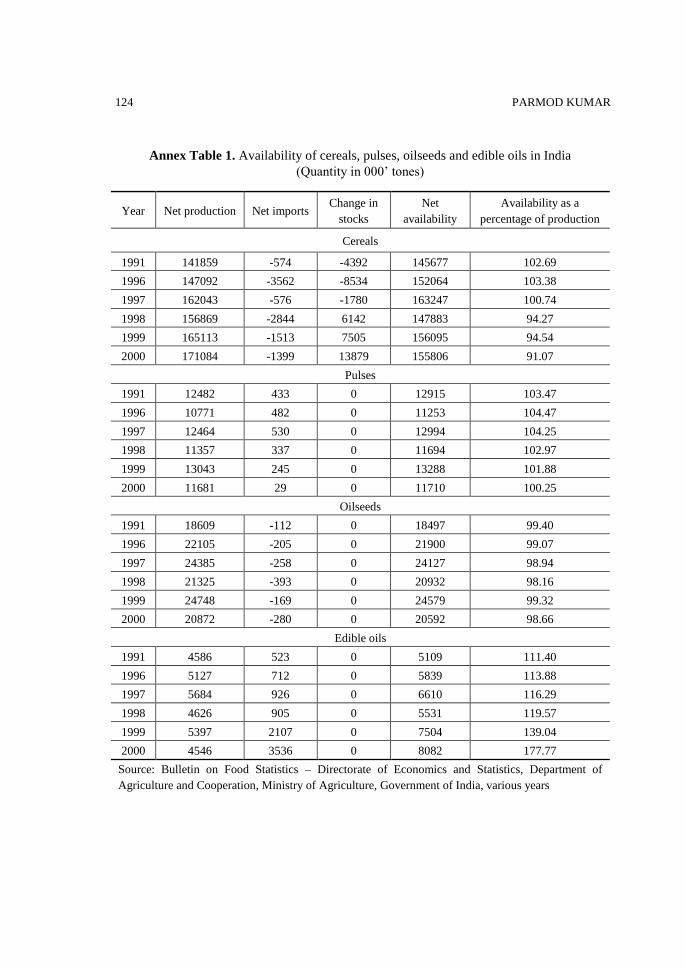
2 The trends in availability (demand) of above commodity complexes were mostly in line with the

trends in production as the net imports (imports-exports) were generally very low in the case of

cereals, pulses and oilseeds. The only exception was edible oils in which case the imported edible oils

have become quite important in the very recent years (see Annex Table 1).

INTER COMMODITY PRICE LINKAGES IN INDIA

105

vanaspati oil, imported edible oil and rice bran oil for the edible oils complex. The data used are

monthly wholesale price indices for the period of April 1990 to March 2002.

2. METHODOLOGICAL FRAMEWORK

Since interdependence among prices is related to their current as well as past levels, we

employ a multivariate co-integration technique to study price interdependence rather than

estimating a structural relationship. A number of studies in the recent past have used time

series techniques to test for price interdependence using co-integration technique3. Unlike the

earlier approaches4 which ignored time series properties (non-stationarity of the data series),

the co-integration methodology captures long run properties also when dealing with the non-

stationary data. The fundamental insight of co-integration analysis is that although many

economic time series may tend to move upwards or downwards over time in a non-stationary

fashion, groups of variables may drift together. If there is a tendency for some linear

relationship to hold between a set of variables over a long period of time, such relationships are

identified with the help of co-integration technique.

However, the simple co-integration tests developed by Granger (1986) and Engle and

Granger (1987) fail to address linkages, which might operate through a third variable and

issues such as endogeneity caused by prices that are simultaneously determined. This is due

to the fact that these methods were developed in a bi-variate framework. To overcome these

limitations, a better and more powerful test for co-integration was developed by Johansen

(1988) and Johanson and Juselius (1990). This test is carried out in a Vector Auto Regressive

mode and is a reduced form method. This test for co-integration is particularly important

when one is dealing with co-integration in a multi-variate framework. The advantage of this

method is that it takes care of both endogeneity and simultaneity problems associated with

simple co-integration tests.

Under Johansen’ procedure, co-integration among the price series is tested using

Johansen’s (1988) maximum likelihood test based on the error-correction representation:

zt = k zt - k + zt-1 + + t (i)

where zt is a vector of I(1) processes. The rank of equals the number of co-integrating

vectors, which is tested by maximum eigenvalue and likelihood ratio test statistics. If there

exist co-movements between prices then there is a possibility that they will trend together in

finding a long run stable equilibrium relationship. This long run stable equilibrium

relationship can be captured by the Granger representation theorem. This theorem states that

if a set of variables are co-integrated, then there exists a valid error correction representation

of the data.

3 See e.g., Stigler and Sherwin (1985), Ardeni (1989), Benson and Faminow (1990), Goodwin and

Schroeder (1991), Asche et al. (1997), Bukenya and Labys (2002), Baffes and Gardner (2003), Rashid

(2004), Krivonos (2004), Jha et al. (2005). 4 See, e.g., Jasdanwalla (1966), Cummings (1967), Lelle (1971), Jones (1968, 1972), Kainth (1982),

Stigler and Sherwin (1985), Neal (1987).

PARMOD KUMAR 106

3. ESTIMATION AND RESULTS

Testing for co-integration at the first step requires testing the order of stationarity of the

variables. Integration tests are prerequisite for co-integration. The order of integration

(existence or absence of non-stationarity) in the time series was checked by the ‘Augmented

Dickey-Fuller (ADF) Test’ (Dickey and Fuller 1979) and ‘Phillips and Perron (PP) Test’

(Phillips and Perron, 1988). To determine the lag length, Akaike’s AIC criterion (Akaike,

1969) was used. The ADF and PP test results for the four commodity complexes are presented

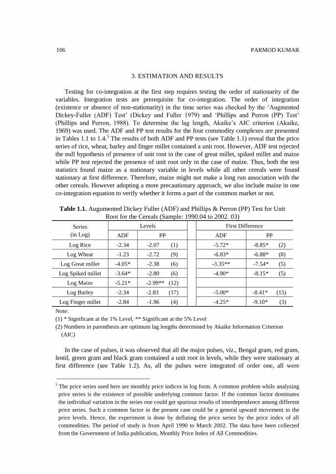
in Tables 1.1 to 1.4.5 The results of both ADF and PP tests (see Table 1.1) reveal that the price

series of rice, wheat, barley and finger millet contained a unit root. However, ADF test rejected

the null hypothesis of presence of unit root in the case of great millet, spiked millet and maize

while PP test rejected the presence of unit root only in the case of maize. Thus, both the test

statistics found maize as a stationary variable in levels while all other cereals were found

stationary at first difference. Therefore, maize might not make a long run association with the

other cereals. However adopting a more precautionary approach, we also include maize in one

co-integration equation to verify whether it forms a part of the common market or not.

Table 1.1. Augumented Dickey Fuller (ADF) and Phillips & Perron (PP) Test for Unit

Root for the Cereals (Sample: 1990.04 to 2002. 03)

Series

(in Log)

Levels

First Difference

ADF PP ADF PP

Log Rice -2.34 -2.07 (1)

-5.72* -8.85* (2)

Log Wheat -1.23 -2.72 (9) -6.83* -6.88* (8)

Log Great millet -4.05* -2.38 (6) -3.35** -7.54* (5)

Log Spiked millet -3.64* -2.80 (6) -4.90* -8.15* (5)

Log Maize -5.21* -2.99** (12)

Log Barley -2.34 -2.83 (17) -5.00* -8.41* (15)

Log Finger millet -2.84 -1.96 (4) -4.25* -9.10* (3)

Note:

(1) * Significant at the 1% Level, ** Significant at the 5% Level

(2) Numbers in parenthesis are optimum lag lengths determined by Akaike Information Criterion

(AIC)

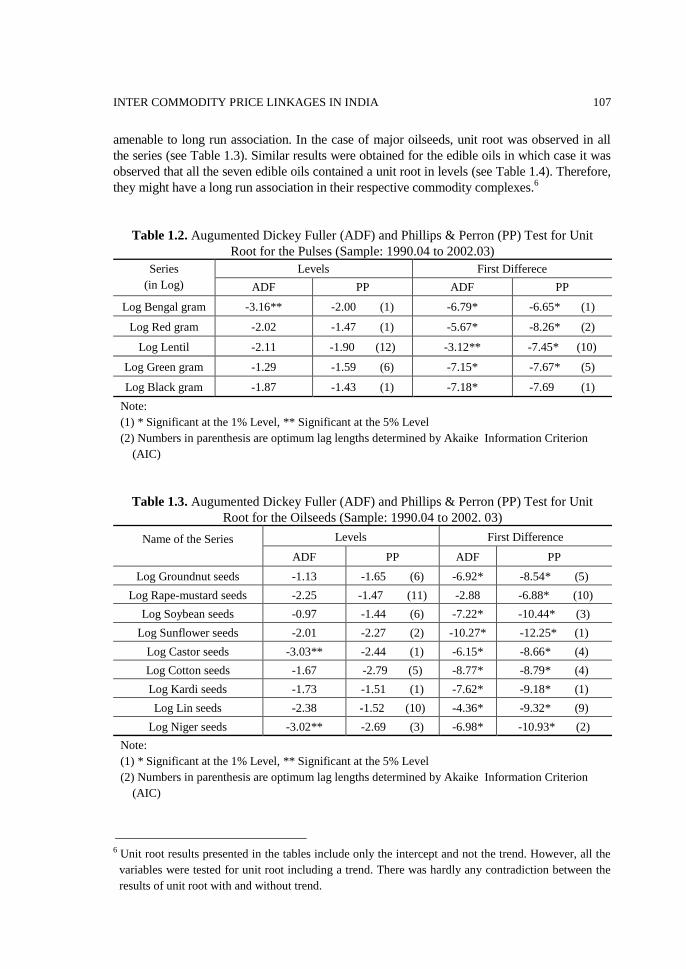
In the case of pulses, it was observed that all the major pulses, viz., Bengal gram, red gram,

lentil, green gram and black gram contained a unit root in levels, while they were stationary at

first difference (see Table 1.2). As, all the pulses were integrated of order one, all were

5 The price series used here are monthly price indices in log form. A common problem while analysing

price series is the existence of possible underlying common factor. If the common factor dominates

the individual variation in the series one could get spurious results of interdependence among different

price series. Such a common factor in the present case could be a general upward movement in the

price levels. Hence, the experiment is done by deflating the price series by the price index of all

commodities. The period of study is from April 1990 to March 2002. The data have been collected

from the Government of India publication, Monthly Price Index of All Commodities.


107

amenable to long run association. In the case of major oilseeds, unit root was observed in all

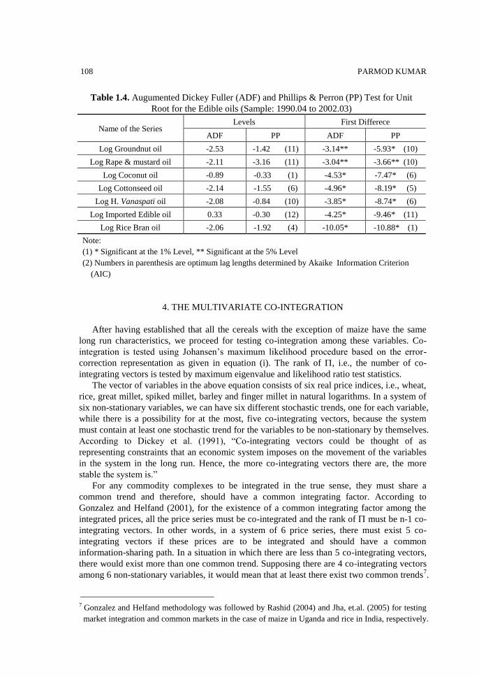
the series (see Table 1.3). Similar results were obtained for the edible oils in which case it was

observed that all the seven edible oils contained a unit root in levels (see Table 1.4). Therefore,

they might have a long run association in their respective commodity complexes.6


Root for the Pulses (Sample: 1990.04 to 2002.03)

Series

(in Log)

Levels First Differece

ADF PP ADF PP

Log Bengal gram -3.16** -2.00 (1) -6.79* -6.65* (1)

Log Red gram -2.02 -1.47 (1) -5.67* -8.26* (2)

Log Lentil -2.11 -1.90 (12) -3.12** -7.45* (10)

Log Green gram -1.29 -1.59 (6) -7.15* -7.67* (5)

Log Black gram -1.87 -1.43 (1) -7.18* -7.69 (1)

Note:



(AIC)


Root for the Oilseeds (Sample: 1990.04 to 2002. 03)

Name of the Series

Levels First Difference

ADF PP ADF PP

Log Groundnut seeds -1.13 -1.65 (6) -6.92* -8.54* (5)

Log Rape-mustard seeds -2.25 -1.47 (11) -2.88 -6.88* (10)

Log Soybean seeds -0.97 -1.44 (6) -7.22* -10.44* (3)

Log Sunflower seeds -2.01 -2.27 (2) -10.27* -12.25* (1)

Log Castor seeds -3.03** -2.44 (1) -6.15* -8.66* (4)

Log Cotton seeds -1.67 -2.79 (5) -8.77* -8.79* (4)

Log Kardi seeds -1.73 -1.51 (1) -7.62* -9.18* (1)

Log Lin seeds -2.38 -1.52 (10) -4.36* -9.32* (9)

Log Niger seeds -3.02** -2.69 (3) -6.98* -10.93* (2)

Note:



(AIC)

6 Unit root results presented in the tables include only the intercept and not the trend. However, all the

variables were tested for unit root including a trend. There was hardly any contradiction between the

results of unit root with and without trend.

PARMOD KUMAR 108


Root for the Edible oils (Sample: 1990.04 to 2002.03)

Name of the Series Levels First Differece

ADF PP ADF PP

Log Groundnut oil -2.53 -1.42 (11) -3.14** -5.93* (10)

Log Rape & mustard oil -2.11 -3.16 (11) -3.04** -3.66** (10)

Log Coconut oil -0.89 -0.33 (1) -4.53* -7.47* (6)

Log Cottonseed oil -2.14 -1.55 (6) -4.96* -8.19* (5)

Log H. Vanaspati oil -2.08 -0.84 (10) -3.85* -8.74* (6)

Log Imported Edible oil 0.33 -0.30 (12) -4.25* -9.46* (11)

Log Rice Bran oil -2.06 -1.92 (4) -10.05* -10.88* (1)

Note:



(AIC)

4. THE MULTIVARIATE CO-INTEGRATION

After having established that all the cereals with the exception of maize have the same

long run characteristics, we proceed for testing co-integration among these variables. Co-

integration is tested using Johansen’s maximum likelihood procedure based on the error-

correction representation as given in equation (i). The rank of , i.e., the number of co-

integrating vectors is tested by maximum eigenvalue and likelihood ratio test statistics.

The vector of variables in the above equation consists of six real price indices, i.e., wheat,

rice, great millet, spiked millet, barley and finger millet in natural logarithms. In a system of

six non-stationary variables, we can have six different stochastic trends, one for each variable,

while there is a possibility for at the most, five co-integrating vectors, because the system

must contain at least one stochastic trend for the variables to be non-stationary by themselves.

According to Dickey et al. (1991), “Co-integrating vectors could be thought of as

representing constraints that an economic system imposes on the movement of the variables

in the system in the long run. Hence, the more co-integrating vectors there are, the more

stable the system is.”

For any commodity complexes to be integrated in the true sense, they must share a

common trend and therefore, should have a common integrating factor. According to

Gonzalez and Helfand (2001), for the existence of a common integrating factor among the

integrated prices, all the price series must be co-integrated and the rank of must be n-1 co-

integrating vectors. In other words, in a system of 6 price series, there must exist 5 co-

integrating vectors if these prices are to be integrated and should have a common

information-sharing path. In a situation in which there are less than 5 co-integrating vectors,

there would exist more than one common trend. Supposing there are 4 co-integrating vectors

among 6 non-stationary variables, it would mean that at least there exist two common trends7.

7 Gonzalez and Helfand methodology was followed by Rashid (2004) and Jha, et.al. (2005) for testing

market integration and common markets in the case of maize in Uganda and rice in India, respectively.


109

In such a situation, some prices could be generated by the first common trend, some by the

second and some by a combination of the first and second trends. Such prices can not be

characterized as integrated because the long run movements in prices would be governed by

different components (Kumar and Sharma 2003).

4.1. Single Common Trend Among Cereals

For searching the commodity combinations that share n-1 co-integrating vectors,

Johansen’s Reduced Rank Vector Auto Regression has been used as discussed above. The

rank of is tested by the maximal eigenvalue test (r), and the trace test (r) based on the

VAR system. The order of VAR (lag) was determined based on Akaike Information

Criterion, Schwarz Bayesian Criterion and Adjusted LR test statistics. Mfit and Eviews

software packages were used for the calculations.8

To determine which particular cereal belongs to the common market, we start with two

variables (wheat and rice) at the first place and test for the number of co-integrating vectors.

If there exists one co-integrating vector that means these two variables (wheat and rice) share

a common trend. In the next step we add an additional cereal. This additional variable would

either share a common trend with the previous two or it would not. If it shares a common

trend, there would exist two co-integrating vectors and this additional variable would belong

to the common market. If we continue to find only one co-integrating vector that means the

additional variable adds another common trend to the system and therefore it does not belong

to the common market. In the latter case, we drop this variable and proceed for checking the

next variable and so on.

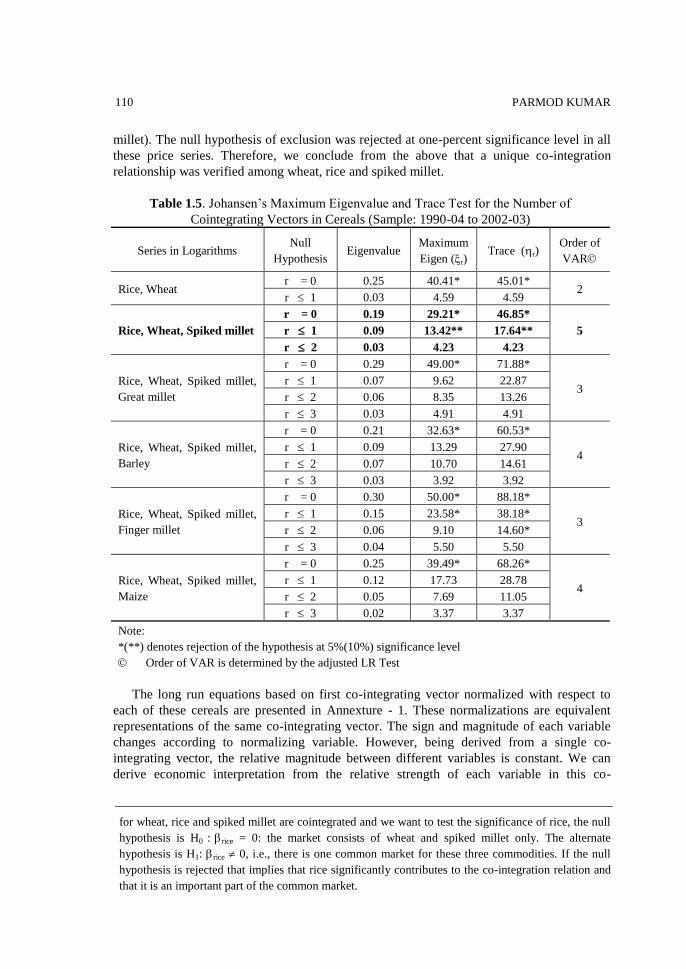
Table 1.5 presents the results of co-integration among the cereals. It is clearly evident

from the results of the table that out of six cereals only wheat, rice and spiked millet shared a

single common market in the long run. Both the maximum eigenvalue test and the trace test

observed two co-integrating vectors (among wheat, rice, and spiked millet). We tried

different sequences among these 6 cereals but the results were invariant to the ordering.

Great millet, barley and finger millet were not found having any long run association with

the other three cereals, viz., wheat, rice and spiked millet. We also included maize in one

equation (although maize was observed as stationary variable) but the results confirmed that

it was not a component of the long run common market.

Since the co-integration tests are not based on a structural model, it is difficult to interpret

the long run elasticities in terms of signs and magnitude given by the co-integration

relationship. However, the relative magnitude of different variables in the co-integrating

relationship can be important to draw some inferences. However, before doing that we test

the significance of different variables in the co-integration vectors. We use the exclusion

tests (Johansen and Juselius 1990) to test the null hypothesis that a particular price series is

not significant in the co-integration relationship by imposing restriction on long run

parameter = 0.9 The CHSQ test statistics were 22.5 (rice), 22.8 (wheat) and 15.3 (spiked

8 As the nature of commodities under analysis was not seasonal, seasonal dummies were not included

in the co-integration equations. We however checked the ECM equations by including three seasonal

(quarter) dummies but observed that in most of the cases their ‘t’ values were not significant and

therefore the final results were estimated without including any seasonal dummies in the case of

ECMs as well. 9 Exclusion tests are imposed as null restrictions on the long-run parameters in . For instance, if prices

PARMOD KUMAR 110

millet). The null hypothesis of exclusion was rejected at one-percent significance level in all

these price series. Therefore, we conclude from the above that a unique co-integration

relationship was verified among wheat, rice and spiked millet.

Table 1.5. Johansen’s Maximum Eigenvalue and Trace Test for the Number of

Cointegrating Vectors in Cereals (Sample: 1990-04 to 2002-03)

Series in Logarithms Null

Hypothesis Eigenvalue

Maximum

Eigen (r) Trace (r)

Order of

VAR

Rice, Wheat r = 0 0.25 40.41* 45.01*

2 r 1 0.03 4.59 4.59

Rice, Wheat, Spiked millet

r = 0 0.19 29.21* 46.85*

5 r 1 0.09 13.42** 17.64**

r 2 0.03 4.23 4.23

Rice, Wheat, Spiked millet,

Great millet

r = 0 0.29 49.00* 71.88*

3 r 1 0.07 9.62 22.87

r 2 0.06 8.35 13.26

r 3 0.03 4.91 4.91


Barley

r = 0 0.21 32.63* 60.53*

4 r 1 0.09 13.29 27.90

r 2 0.07 10.70 14.61

r 3 0.03 3.92 3.92


Finger millet

r = 0 0.30 50.00* 88.18*

3 r 1 0.15 23.58* 38.18*

r 2 0.06 9.10 14.60*

r 3 0.04 5.50 5.50


Maize

r = 0 0.25 39.49* 68.26*

4 r 1 0.12 17.73 28.78

r 2 0.05 7.69 11.05

r 3 0.02 3.37 3.37

Note:

*(**) denotes rejection of the hypothesis at 5%(10%) significance level

Order of VAR is determined by the adjusted LR Test

The long run equations based on first co-integrating vector normalized with respect to

each of these cereals are presented in Annexture - 1. These normalizations are equivalent

representations of the same co-integrating vector. The sign and magnitude of each variable

changes according to normalizing variable. However, being derived from a single co-

integrating vector, the relative magnitude between different variables is constant. We can

derive economic interpretation from the relative strength of each variable in this co-

for wheat, rice and spiked millet are cointegrated and we want to test the significance of rice, the null

hypothesis is H0 : rice = 0: the market consists of wheat and spiked millet only. The alternate

hypothesis is H1: rice 0, i.e., there is one common market for these three commodities. If the null

hypothesis is rejected that implies that rice significantly contributes to the co-integration relation and

that it is an important part of the common market.


111

integrating relationship.

Considering the equations for cereals in Annexture -1, the parameter for wheat was 3.65

times higher than that of spiked millet in equation (i). The parameter of rice was 5.96 times

higher than that of spiked millet in equation (ii). This suggests that the interdependency

between wheat-rice was relatively stronger than that of either wheat-spiked millet or rice-

spiked millet. In equation (iii) the parameter of rice was 1.61 times higher than that of wheat

suggesting that the interdependency of rice-spiked millet was greater than that of wheat-

spiked millet. By putting these preferences together, we get an ordering of the relative

strength of the variables suggested by our long run co-integration relationship. Combining

the results of the above three, we get the combination of substitutes as rice-wheat rice-

spiked millet wheat-spiked millet. Thus we conclude that there was price parity

equilibrium in the cereals market excluding great millet, maize, barley and finger millet. In

the long run the interdependence was evident in the order of rice, wheat and spiked millet.

4.2. Single Common Trend Among Pulses

Searching for a common market in the pulses, we considered five main pulses namely,

Bengal gram, black gram, red gram, lentil and green gram. Out of these five pulses only

lentil, green gram and Bengal gram were observed to belong to a single common market.

Table 1.6 shows that only two co-integrating vectors were accepted by trace and maximum

eigenvalue tests among lentil, green gram and Bengal gram. The remaining two pulses

namely, red gram and black gram did not belong to the common market. Using exclusion

tests to further verify the presence of a particular series in the co-integration relationship as

in the case of cereals, the calculated CHSQ test statistics were 20.7 (green gram), 14.0

(lentil) and 14.1 (Bengal gram). The null hypothesis of exclusion was rejected at one-percent


Cointegrating Vectors in Pulses (Sample: 1990-04 to 2002-03)



Maximum

Eigen (r) Trace (r)

Order of

VAR

Lentil, Green gram r = 0 0.16 25.24* 30.87*

2 r 1 0.04 5.63 5.63

Lentil, Green gram,

Bengal gram

r = 0 0.17 25.62* 49.13*

2 r 1 0.13 19.34* 23.51**

r 2 0.03 4.17 4.17

Lentil, Green gram,

Bengal gram, Red gram

r = 0 0.16 25.32** 51.13*

2 r 1 0.13 19.28** 25.81

r 2 0.03 3.99 6.52

r 3 0.02 2.53 2.53

Lentil, Green gram,

Bengal gram, Black gram

r = 0 0.20 31.19* 65.24*

2 r 1 0.14 21.61 34.04

r 2 0.06 8.19 12.43

r 2 0.03 4.24 4.24

Note:



PARMOD KUMAR 112

significance level leading to the conclusion that lentil, green gram and Bengal gram had a

unique long run association.

The long run equations based on first co-integrating vector normalized with respect to

each of these pulses are given in Annexture 1. In the next step we derive the order of

preference for these pulses using the relative strength of each variable in the normalized

equations. It is evident from these equations that the parameter of green gram was 9.16 times

higher than that of Bengal gram in equation (i). The parameter of lentil was 3.18 times higher

than that of Bengal gram in equation (ii). This implies that the association of green gram-

lentil was stronger than that of either green gram-Bengal gram or lentil-Bengal gram. In

equation (iii) the parameter of green gram was 2.84 times higher than that of lentil

suggesting that the interdependency of green gram-Bengal gram was greater than that of

lentil-Bengal gram. Combining the results of the above three, we get the desired preference

of substitutes as green gram-lentil green gram-Bengal gram lentil-Bengal gram.

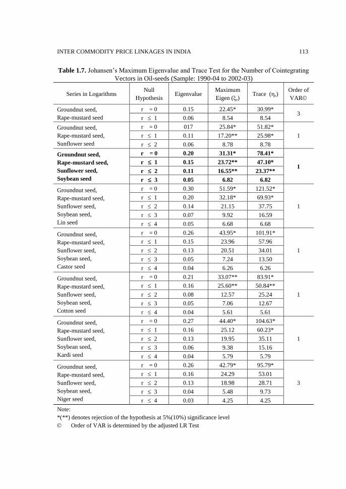
4.3. Single Common Trend Among Oilseeds

Among 9 major oilseeds only groundnut, mustard, sunflower and soybean were found to

belong to a common market. It is evident from Table 1.7 that only 3 co-integrating vectors

were accepted by both maximum eigenvalue and trace tests. As was mentioned in the

previous section, these four oilseeds also constituted the major share (around 90 percent) of

total oilseeds production. During 1999-00, the share of groundnut, soybean and rapeseed

mustard in total 9 oilseeds’ production was 25, 33 and 29 percent, respectively. However,

sunflower had a meager share of 4 percent.

The results of exclusion tests further corroborate the presence of all the four oilseeds in

the common market. The calculated CHSQ test statistics were 12.7, 18.8, 17.5 and 15.9 for

soybean, sunflower, mustard and groundnut respectively, thus rejecting the null hypothesis

of exclusion at one-percent significance level. The remaining 5 oilseeds namely, linseed,

castor seed, cotton seed, niger seed and kardi seed having a production share of only 5

percent were not observed to have any common long run path with the above 4 major

oilseeds. In the subsequent sections we would see the short run association among all these 9

oilseeds.

Based on the set of normalized equations of the first vector of co-integration (see

Annexture-1), the order of preference for these four oilseeds is given in the following lines:

The parameter for mustard was 1.31 times higher than that of sunflower in equation (i). The

parameter of soybean was 1.07 times higher than that of sunflower in equation (ii). This

implies that the association of mustard-soybean was stronger than that of either mustard-

sunflower or soybean-sunflower. In equation (iii) the parameter of mustard was 1.24 times

higher than that of soybean suggesting that the interdependency of mustard-sunflower was

greater than that of soybean-sunflower. Combining the results of the above three, we get the

combination of substitutes as mustard-soybean mustard-sunflower soybean-sunflower.

Similarly, we can find out the order of preference among the combinations of mustard,

soybean and groundnut. The parameter of mustard in equation (iv) was 4.73 times higher

than that of groundnut while parameter of soybean was 3.86 times higher than that of

groundnut in equation (ii). This suggests that the interdependence between mustard-soybean

was much higher than that of mustard-groundnut or soybean- groundnut. From equation (iii)

it is discernible that parameter of mustard was 1.23 times higher than that of soybean thus

concluding in the order of mustard-soybean mustard-groundnut soybean-groundnut.


113

Table 1.7. Johansen’s Maximum Eigenvalue and Trace Test for the Number of Cointegrating

Vectors in Oil-seeds (Sample: 1990-04 to 2002-03)



Maximum

Eigen (r) Trace (r)

Order of

VAR

Groundnut seed,

Rape-mustard seed

r = 0 0.15 22.45* 30.99* 3

r 1 0.06 8.54 8.54

Groundnut seed,

Rape-mustard seed,

Sunflower seed

r = 0 017 25.84* 51.82*

1 r 1 0.11 17.20** 25.98*

r 2 0.06 8.78 8.78

Groundnut seed,

Rape-mustard seed,

Sunflower seed,

Soybean seed

r = 0 0.20 31.31* 78.41*

1 r 1 0.15 23.72** 47.10*

r 2 0.11 16.55** 23.37**

r 3 0.05 6.82 6.82

Groundnut seed,

Rape-mustard seed,

Sunflower seed,

Soybean seed,

Lin seed

r = 0 0.30 51.59* 121.52*

1

r 1 0.20 32.18* 69.93*

r 2 0.14 21.15 37.75

r 3 0.07 9.92 16.59

r 4 0.05 6.68 6.68

Groundnut seed,

Rape-mustard seed,

Sunflower seed,

Soybean seed,

Castor seed

r = 0 0.26 43.95* 101.91*

1

r 1 0.15 23.96 57.96

r 2 0.13 20.51 34.01

r 3 0.05 7.24 13.50

r 4 0.04 6.26 6.26

Groundnut seed,

Rape-mustard seed,

Sunflower seed,

Soybean seed,

Cotton seed

r = 0 0.21 33.07** 83.91*

1

r 1 0.16 25.60** 50.84**

r 2 0.08 12.57 25.24

r 3 0.05 7.06 12.67

r 4 0.04 5.61 5.61

Groundnut seed,

Rape-mustard seed,

Sunflower seed,

Soybean seed,

Kardi seed

r = 0 0.27 44.40* 104.63*

1

r 1 0.16 25.12 60.23*

r 2 0.13 19.95 35.11

r 3 0.06 9.38 15.16

r 4 0.04 5.79 5.79

Groundnut seed,

Rape-mustard seed,

Sunflower seed,

Soybean seed,

Niger seed

r = 0 0.26 42.79* 95.79*

3

r 1 0.16 24.29 53.01

r 2 0.13 18.98 28.71

r 3 0.04 5.48 9.73

r 4 0.03 4.25 4.25

Note:



PARMOD KUMAR 114

Finally, from equation (ii) or (iv) we could calculate that the parameter of sunflower was

3.62 times higher than that of groundnut suggesting that the association between mustard-

sunflower and soybean-sunflower was greater than that of mustard-groundnut and soybean-

goundnut. Now putting these preferences together we get an ordering of the relative strength

of the variables suggested by our long run co-integration relationship as: mustard-soybean

mustard-sunflower soybean-sunflower mustard-groundnut soybean-groundnut

sunflower-groundnut.

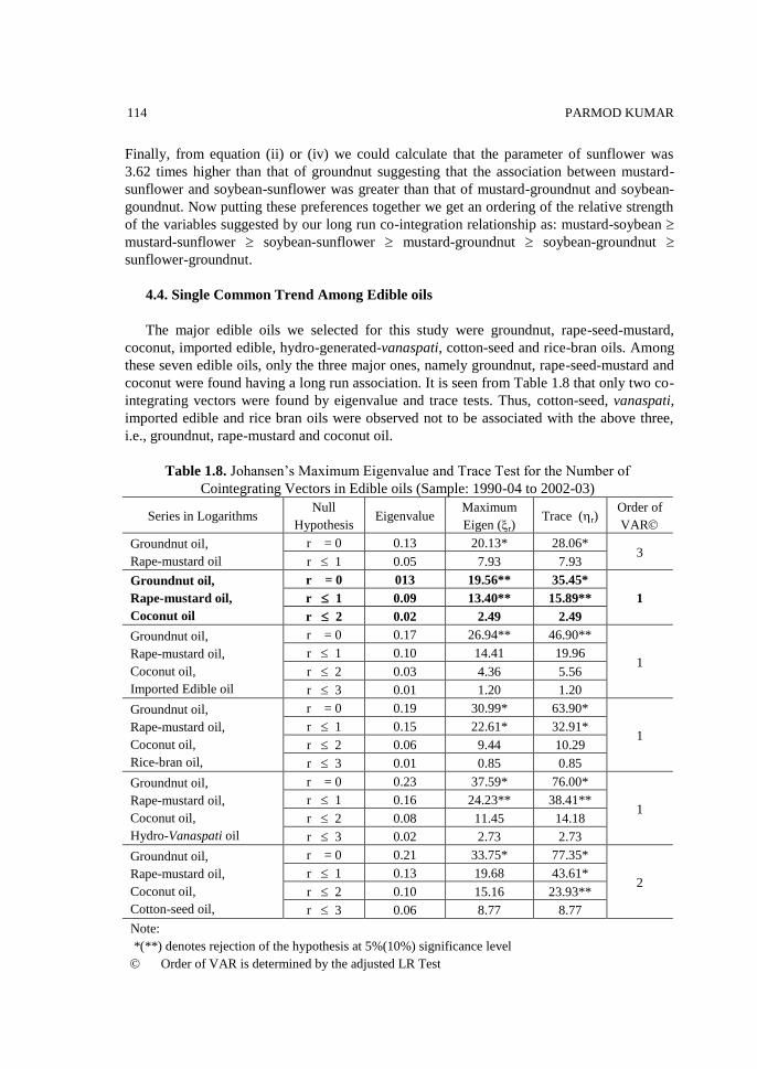
4.4. Single Common Trend Among Edible oils

The major edible oils we selected for this study were groundnut, rape-seed-mustard,

coconut, imported edible, hydro-generated-vanaspati, cotton-seed and rice-bran oils. Among

these seven edible oils, only the three major ones, namely groundnut, rape-seed-mustard and

coconut were found having a long run association. It is seen from Table 1.8 that only two co-

integrating vectors were found by eigenvalue and trace tests. Thus, cotton-seed, vanaspati,

imported edible and rice bran oils were observed not to be associated with the above three,

i.e., groundnut, rape-mustard and coconut oil.


Cointegrating Vectors in Edible oils (Sample: 1990-04 to 2002-03)



Maximum

Eigen (r) Trace (r)

Order of

VAR

Groundnut oil,

Rape-mustard oil

r = 0 0.13 20.13* 28.06* 3

r 1 0.05 7.93 7.93

Groundnut oil,

Rape-mustard oil,

Coconut oil

r = 0 013 19.56** 35.45*

1 r 1 0.09 13.40** 15.89**

r 2 0.02 2.49 2.49

Groundnut oil,

Rape-mustard oil,

Coconut oil,

Imported Edible oil

r = 0 0.17 26.94** 46.90**

1 r 1 0.10 14.41 19.96

r 2 0.03 4.36 5.56

r 3 0.01 1.20 1.20

Groundnut oil,

Rape-mustard oil,

Coconut oil,

Rice-bran oil,

r = 0 0.19 30.99* 63.90*

1 r 1 0.15 22.61* 32.91*

r 2 0.06 9.44 10.29

r 3 0.01 0.85 0.85

Groundnut oil,

Rape-mustard oil,

Coconut oil,

Hydro-Vanaspati oil

r = 0 0.23 37.59* 76.00*

1 r 1 0.16 24.23** 38.41**

r 2 0.08 11.45 14.18

r 3 0.02 2.73 2.73

Groundnut oil,

Rape-mustard oil,

Coconut oil,

Cotton-seed oil,

r = 0 0.21 33.75* 77.35*

2 r 1 0.13 19.68 43.61*

r 2 0.10 15.16 23.93**

r 3 0.06 8.77 8.77

Note:




115

The CHSQ (exclusion) test further confirmed the presence of these three edible oils in the

common market. The hypothesis was rejected at one percent significance level in all the

three edible oils as the estimated test statistics were 7.6 (coconut oil), 11.1 (mustard oil) and

10.7 (groundnut oil). The order of preference drawn from the set of normalized equations (as

given in Annexture-1) of the first vector stood as – Mustard-coconut > mustard-groundnut >

coconut-groundnut.

5. THE ERROR-CORRECTION MODEL

An explanation for the long run interdependence among the variables lies in the short run

dynamics. One would like to know the intertwined relationship in the short run giving way to

a long run association. The relationship was estimated by error-correction model (Engle and

Granger 1987). The advantage of error-correction model is that it allows for the short run

dynamics as well as an assessment for the degree of convergence towards the long run

relation as shown by the co-integration. The model is formulated by including the respective

variables in their first difference, their lagged values and the lagged residuals from the co-

integration equations.

5.1. Cereals

Before starting the discussion, it is essential to note that the coarse grains namely, great

millet, barley and finger millet, which were observed not belonging to the common market in

the co-integration analysis have been included in the short run analysis of error-correction.

Further, to check short run association of maize with the other cereals, the former was

included in the ECM equations. However, maize was included in levels as this variable was

observed as stationary, the other variables namely, great millet, barley and finger millet were

included in their first difference as latter were all not stationary variables. The results for the

cereals show that the estimates of the error correction coefficients were highly significant

and their signs were negative (Table 1.9). This implies that the short run price movements

along the long run equilibrium path were stable. The coefficients of the error correction

terms indicate the speed of convergence to the long run growth path as a result of a shock in

their own prices. The estimated coefficients show that the speed of adjustment to a shock in

their own prices was rather slow in the case of rice as compared to wheat and spiked millet.

Any shock in prices took about 3-4 weeks adjustment period to get back to the long run path

in the case of rice and 2-3 weeks period in the case of wheat and spiked millet in a months’

time period.

The coefficients of the own lagged prices and prices of the substitutes reveal that rice

price was affected by wheat, with a two month lag, while the impact of its own price took

place with one month delay. With respect to coarse grains, although barley and finger millet

did not share a common path with rice in the long run, they were significant substitutes in the

short run (see Table 1.9). Wheat price was affected by its own lagged price and also by the

lagged prices of other two cereals, i.e., rice with a lag of two months and spiked millet with a

lag of one month. The movements in prices of great millet and barley also caused variation in

wheat prices in the short run, though in the long run they did not share a common path. In the

case of spiked millet, there was a significant impact of change in its own price and the price

of wheat with a month lag while finger millet and maize affected its price only in the short

PARMOD KUMAR 116

run.

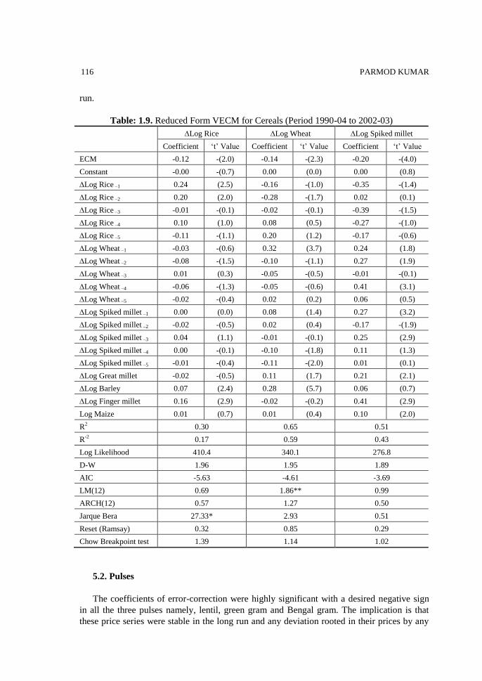
Table: 1.9. Reduced Form VECM for Cereals (Period 1990-04 to 2002-03)

Log Rice Log Wheat Log Spiked millet

Coefficient ‘t’ Value Coefficient ‘t’ Value Coefficient ‘t’ Value

ECM -0.12 -(2.0) -0.14 -(2.3) -0.20 -(4.0)

Constant -0.00 -(0.7) 0.00 (0.0) 0.00 (0.8)

Log Rice –1 0.24 (2.5) -0.16 -(1.0) -0.35 -(1.4)

Log Rice –2 0.20 (2.0) -0.28 -(1.7) 0.02 (0.1)

Log Rice –3 -0.01 -(0.1) -0.02 -(0.1) -0.39 -(1.5)

Log Rice –4 0.10 (1.0) 0.08 (0.5) -0.27 -(1.0)

Log Rice –5 -0.11 -(1.1) 0.20 (1.2) -0.17 -(0.6)

Log Wheat –1 -0.03 -(0.6) 0.32 (3.7) 0.24 (1.8)

Log Wheat –2 -0.08 -(1.5) -0.10 -(1.1) 0.27 (1.9)

Log Wheat –3 0.01 (0.3) -0.05 -(0.5) -0.01 -(0.1)

Log Wheat –4 -0.06 -(1.3) -0.05 -(0.6) 0.41 (3.1)

Log Wheat –5 -0.02 -(0.4) 0.02 (0.2) 0.06 (0.5)

Log Spiked millet –1 0.00 (0.0) 0.08 (1.4) 0.27 (3.2)

Log Spiked millet –2 -0.02 -(0.5) 0.02 (0.4) -0.17 -(1.9)

Log Spiked millet –3 0.04 (1.1) -0.01 -(0.1) 0.25 (2.9)

Log Spiked millet –4 0.00 -(0.1) -0.10 -(1.8) 0.11 (1.3)

Log Spiked millet –5 -0.01 -(0.4) -0.11 -(2.0) 0.01 (0.1)

Log Great millet -0.02 -(0.5) 0.11 (1.7) 0.21 (2.1)

Log Barley 0.07 (2.4) 0.28 (5.7) 0.06 (0.7)

Log Finger millet 0.16 (2.9) -0.02 -(0.2) 0.41 (2.9)

Log Maize 0.01 (0.7) 0.01 (0.4) 0.10 (2.0)

R2 0.30 0.65 0.51

R-2

0.17 0.59 0.43

Log Likelihood 410.4 340.1 276.8

D-W 1.96 1.95 1.89

AIC -5.63 -4.61 -3.69

LM(12) 0.69 1.86** 0.99

ARCH(12) 0.57 1.27 0.50

Jarque Bera 27.33* 2.93 0.51

Reset (Ramsay) 0.32 0.85 0.29

Chow Breakpoint test 1.39 1.14 1.02

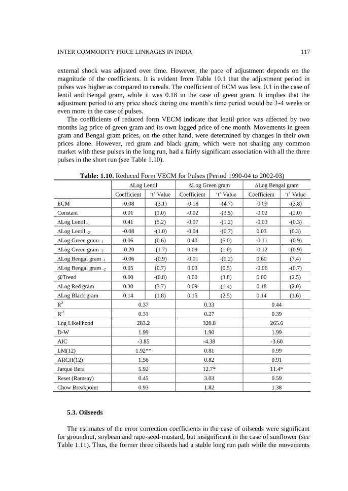
5.2. Pulses

The coefficients of error-correction were highly significant with a desired negative sign

in all the three pulses namely, lentil, green gram and Bengal gram. The implication is that

these price series were stable in the long run and any deviation rooted in their prices by any


117

external shock was adjusted over time. However, the pace of adjustment depends on the

magnitude of the coefficients. It is evident from Table 10.1 that the adjustment period in

pulses was higher as compared to cereals. The coefficient of ECM was less, 0.1 in the case of

lentil and Bengal gram, while it was 0.18 in the case of green gram. It implies that the

adjustment period to any price shock during one month’s time period would be 3-4 weeks or

even more in the case of pulses.

The coefficients of reduced form VECM indicate that lentil price was affected by two

months lag price of green gram and its own lagged price of one month. Movements in green

gram and Bengal gram prices, on the other hand, were determined by changes in their own

prices alone. However, red gram and black gram, which were not sharing any common

market with these pulses in the long run, had a fairly significant association with all the three

pulses in the short run (see Table 1.10).

Table: 1.10. Reduced Form VECM for Pulses (Period 1990-04 to 2002-03)

Log Lentil Log Green gram Log Bengal gram


ECM -0.08 -(3.1) -0.18 -(4.7) -0.09 -(3.8)

Constant 0.01 (1.0) -0.02 -(3.5) -0.02 -(2.0)

Log Lentil –1 0.41 (5.2) -0.07 -(1.2) -0.03 -(0.3)

Log Lentil –2 -0.08 -(1.0) -0.04 -(0.7) 0.03 (0.3)

Log Green gram –1 0.06 (0.6) 0.40 (5.0) -0.11 -(0.9)

Log Green gram –2 -0.20 -(1.7) 0.09 (1.0) -0.12 -(0.9)

Log Bengal gram –1 -0.06 -(0.9) -0.01 -(0.2) 0.60 (7.4)

Log Bengal gram –2 0.05 (0.7) 0.03 (0.5) -0.06 -(0.7)

@Trend 0.00 -(0.8) 0.00 (3.8) 0.00 (2.5)

Log Red gram 0.30 (3.7) 0.09 (1.4) 0.18 (2.0)

Log Black gram 0.14 (1.8) 0.15 (2.5) 0.14 (1.6)

R2 0.37 0.33 0.44

R-2

0.31 0.27 0.39


D-W 1.99 1.90 1.99

AIC -3.85 -4.38 -3.60

LM(12) 1.92** 0.81 0.99

ARCH(12) 1.56 0.82 0.91

Jarque Bera 5.92 12.7* 11.4*

Reset (Ramsay) 0.45 3.03 0.59

Chow Breakpoint 0.93 1.82 1.38

5.3. Oilseeds

The estimates of the error correction coefficients in the case of oilseeds were significant

for groundnut, soybean and rape-seed-mustard, but insignificant in the case of sunflower (see

Table 1.11). Thus, the former three oilseeds had a stable long run path while the movements

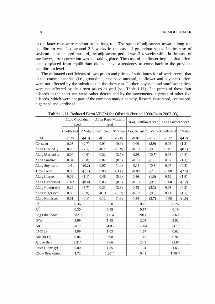
PARMOD KUMAR 118

in the latter case were random in the long run. The speed of adjustment towards long run

equilibrium was fast, around 2-3 weeks in the case of groundnut seeds. In the case of

soybean and rape-seed-mustard, the adjustment period was 3-4 weeks while in the case of

sunflower, error correction was not taking place. The case of sunflower implies that prices

once displaced from equilibrium did not have a tendency to come back to the previous

equilibrium level.

The estimated coefficients of own prices and prices of substitutes for oilseeds reveal that

in the common market (i.e., groundnut, rape-seed-mustard, sunflower and soybean) prices

were not affected by the substitutes in the short run. Further, soybean and sunflower prices

were not affected by their own prices as well (see Table 1.11). The prices of these four

oilseeds in the short run were rather determined by the movements in prices of other five

oilseeds, which were not part of the common market namely, linseed, castorseed, cottonseed,

nigerseed and kardiseed.

Table: 1.11. Reduced Form VECM for Oilseeds (Period 1990-04 to 2002-03)

Log Groundnut

seed

Log Rape-Mustard

seed Log Sunflower seed Log Soybean seed

Coefficient ‘t’ Value Coefficient ‘t’ Value Coefficient ‘t’ Value Coefficient ‘t’ Value

ECM -0.25 -(4.3) -0.06 -(2.0) -0.07 -(1.2) -0.12 -(4.2)

Constant 0.03 (2.7) 0.01 (0.9) 0.06 (2.9) 0.02 (1.3)

Log Ground –1 0.20 (2.1) -0.09 -(0.9) -0.10 -(0.5) -0.01 -(0.1)

Log Mustard –1 0.00 (0.0) 0.22 (2.7) -0.08 -(0.5) 0.08 (0.8)

Log Sunflwr –1 0.04 (0.8) 0.02 (0.5) -0.10 -(1.0) 0.07 (1.1)

Log Soybean–1 -0.01 -(0.2) 0.07 (1.0) -0.11 -(0.8) 0.07 (0.8)

Time Trend 0.00 -(1.7) 0.00 -(1.6) -0.00 -(2.5) -0.00 -(2.5)

Log Linseed 0.09 (1.1) 0.46 (5.9) 0.16 (1.0) 0.19 (1.9)

Log Castorseed -0.02 -(0.4) 0.05 (0.8) -0.10 -(0.9) -0.08 -(1.2)

Log Cottonseed 0.29 (3.7) 0.23 (2.8) 0.53 (3.3) 0.03 (0.3)

Log Nigerseed 0.05 (0.9) -0.01 -(0.2) -0.10 -(0.9) 0.11 (1.5)

Log Kardiseed 0.01 (0.1) 0.12 (1.9) 0.34 (2.7) -0.08 -(1.0)

R2 0.36 0.50 0.25 0.26

R-2

0.30 0.45 0.17 0.19

Log Likelihood 302.0 300.4 201.8 266.1

D-W 1.99 1.85 2.03 2.02

AIC -4.06 -4.03 -2.64 -3.55

LM(12) 1.09 1.03 1.57 0.62

ARCH(12) 0.84 0.98 1.43 0.97

Jarque Bera 9.51* 5.66 2.43 21.6*

Reset (Ramsay) 0.00 1.35 1.04 1.63

Chow Breakpoint 1.72 1.80** 0.41 1.96**


119

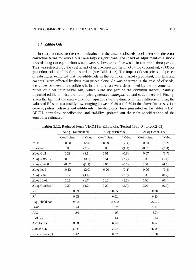
5.4. Edible Oils

In sharp contrast to the results obtained in the case of oilseeds, coefficients of the error

correction terms for edible oils were highly significant. The speed of adjustment of a shock

towards long run equilibrium was however, slow, about four weeks in a month’s time period.

This was reflected by the coefficient of error-correction term, -0.04 for coconut oil, -0.08 for

groundnut oil and -0.09 for mustard oil (see Table 1.12). The impact of own prices and prices

of substitutes exhibited that the edible oils in the common market (groundnut, mustard and

coconut) were affected by their own prices alone. As was observed in the case of oilseeds,

the prices of these three edible oils in the long run were determined by the movements in

prices of other four edible oils, which were not part of the common market, namely,

imported edible oil, rice-bran oil, hydro-generated vanaspati oil and cotton-seed oil. Finally,

given the fact that the error-correction equations were estimated in first difference form, the

values of R2 were reasonably low, ranging between 0.30 and 0.70 in the above four cases, i.e.,

cereals, pulses, oilseeds and edible oils. The diagnostic tests presented in the tables – LM,

ARCH, normality, specification and stability- pointed out the right specifications of the

equations estimated.

Table: 1.12. Reduced Form VECM for Edible oils (Period 1990-04 to 2002-03)

Log Groundnut oil Log Mustard oil Log Coconut oil


ECM -0.08 -(2.4) -0.09 -(2.9) -0.04 -(3.2)

Constant 0.00 (0.6) 0.00 -(0.8) -0.01 -(1.8)

Log Goil –1 0.28 (3.5) 0.05 (0.6) -0.07 -(0.7)

Log Rmoil –1 -0.01 -(0.2) 0.51 (7.2) 0.09 (1.1)

Log Cocoil –1 -0.07 -(1.1) 0.05 (0.7) 0.37 (4.5)

Log Ieoil -0.13 -(2.0) -0.20 -(3.2) -0.06 -(0.8)

Log Rboil 0.17 (4.1) 0.16 (3.8) 0.03 (0.7)

Log Hvoil 0.19 (1.7) 0.13 (1.1) 0.06 (0.4)

Log Cseedoil 0.23 (3.2) 0.23 (3.3) 0.04 (0.5)

R2 0.39 0.55 0.28

R-2

0.35 0.52 0.23


D-W 1.94 1.87 2.11

AIC -4.06 -4.07 -3.74

LM(12) 1.01 1.13 1.13

ARCH(12) 0.69 0.84 0.54

Jarque Bera 37.8* 2.04 47.5*

Reset (Ramsay) 1.42 0.37 1.88

PARMOD KUMAR 120

Figure 1.1: Long Term Adjustment Path

-2.50

-2.00

-1.50

-1.00

-0.50

0.00

0.50

1.00

1.50

1990:04

1991:04

1992:04

1993:04

1994:04

1995:04

1996:04

1997:04

1998:04

1999:04

2000:04

2001:04

Cereals Pulses Oil seeds Edible oils

The results of co-integration and error-correction are summarized in Figure 1.1. The

figure presents a comparative picture of long run path of price adjustments for cereals, pulses,

oilseeds and edible oils. It is clearly evident from the plots that diversions across the long-run

path were highest in the case of oilseeds. It was seen in the previous section that the

coefficients of error-correction in oilseed crops were either insignificant or very small except

that of groundnut. As a result, the magnitude of diversions across the long run path was high

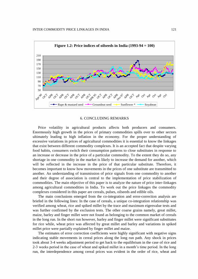
in oilseeds. Further, it is apparent from Figure 1.1 that in the late 1990’s, prices were drifting

away from the long run equilibrium path. The drift in prices might have occurred due to the

exceptional increase in prices of oilseeds during the year 1998-99. The oilseed market was

severely hit during 1998-99 due to loss of human lives because of dropsy disease that broke

out in many states in India as a result of adulterated mustard oil. A majority of state

governments banned the sale of loose mustard oil, which caused disturbance in the oilseeds

market10

. Nonetheless, the drift is not visible in the case of edible oils probably because of

the presence of imported edible oils, which partially evened out the rise in prices of mustard

and other edible oils. The diversions were least for cereals and to some extent for pulses,

evidently because no such disturbance happened in their case. Moreover, there is an effective

procurement and minimum support price policy adopted by the Government of India,

absorbing price shocks in the case of cereals’ while oilseeds and edible oils depend entirely

on the market situation.

10 However, the drift in prices was only an aberration and was not a structural break as it occurred for a

very small period and the prices returned to their normal level within a short span of time. Moreover,

the drift was most acute only in the case of mustard seed (Figure 1.2). The ECM equations were tested

for structural break by employing the CUSUM squared test as well as Chow’s break point test

(CUSUM graphs are not presented in the paper while they are available with the author). Even in the

case of mustard seed, it was observed that CUSUM graph did not display any structural break.


121

Figure 1.2: Price indices of oilseeds in India (1993-94 = 100)

50

70

90

110

130

150

170

190

210

Apr

90

OCT

APR

OCT

APR

OCT

APR

OCT

APR

OCT

APR

95

OCT

APR

OCT

APR

Oct

-97

APR

OCT

Apr O

ctA

pr Oct

Apr O

ct

Rape & mustard seed Groundnut seed Sunflower * Soyabean

6. CONCLUDING REMARKS

Price volatility in agricultural products affects both producers and consumers.

Enormously high growth in the prices of primary commodities spills over to other sectors

ultimately leading to high inflation in the economy. For the proper understanding of

excessive variations in prices of agricultural commodities it is essential to know the linkages

that exist between different commodity complexes. It is an accepted fact that despite varying

food habits, consumers switch their consumption patterns to close substitutes in response to

an increase or decrease in the price of a particular commodity. To the extent they do so, any

shortage in one commodity in the market is likely to increase the demand for another, which

will be reflected in the increase in the price of that particular substitute. Therefore, it

becomes important to know how movements in the prices of one substitute are transmitted to

another. An understanding of transmission of price signals from one commodity to another

and their degree of association is central to the implementation of price stabilization of

commodities. The main objective of this paper is to analyze the nature of price inter-linkages

among agricultural commodities in India. To work out the price linkages the commodity

complexes considered in this paper are cereals, pulses, oilseeds and edible oils.

The main conclusions emerged from the co-integration and error-correction analysis are

briefed in the following lines: In the case of cereals, a unique co-integration relationship was

verified among wheat, rice and spiked millet by the trace and maximum eigenvalue tests and

was further confirmed by the exclusion tests. The other coarse grains namely, great millet,

maize, barley and finger millet were not found as belonging to the common market of cereals

in the long run. In the short run however, barley and finger millet were significant substitutes

for rice while, wheat price was affected by great millet and barley and variations in spiked

millet price were partially explained by finger millet and maize.

The estimates of error correction coefficients were highly significant with negative signs

indicating stable movements in cereal prices along the long run path. Any shock in prices

took about 3-4 weeks adjustment period to get back to the equilibrium in the case of rice and

2-3 weeks period in the case of wheat and spiked millet in a month’s time period. In the long

run, the interdependence among cereal prices was evident in the order of rice, wheat and

PARMOD KUMAR 122

spiked millet and the combination of substitutes were observed as rice-wheat rice-spiked

millet wheat-spiked millet.

Among pulses, only lentil, green gram and Bengal gram had a long run co-integration

relation and thus formed a single common market of pulses. The other two pulses, namely,

red gram and black gram did not belong to the common market. Nonetheless, although the

latter two pulses did not share any common market with former three in the long run, they

had a fairly significant association with the above three pulses in the short run. The

coefficients of error-correction were highly significant with a desired negative sign

indicating stable price movements. However, the period of adjustment in pulses was higher

compared to cereals (about 3-4 weeks or even more). The order of preference for substitutes

was derived as green gram-lentil green gram-Bengal gram lentil-Bengal gram.

Among nine major oilseeds only groundnut, mustard, sunflower and soybean belonged to

a common market as only three co-integrating vectors were accepted by both maximum

eigenvalue and trace tests. The remaining five oilseeds, namely, linseed, castor seed, cotton

seed, niger seed and kardi seed with a production share of only 5 percent were not observed

sharing any common market with the above four oilseeds, although in the short run they

governed the price movements of the above four oilseeds. The estimates of the error

correction coefficients in the case of oilseeds were significant for groundnut, soybean and

rape-seed-mustard, but insignificant in the case of sunflower. Thus, the former three oilseeds

had a stable long run path while the movements in the latter case were random and no error-

correction was taking place in this case. The ordering of the relative strength of oilseeds was

found as, mustard-soybean mustard-sunflower soybean-sunflower mustard-groundnut

soybean-groundnut sunflower-groundnut.

In the case of edible oils, only three major ones namely, groundnut, rape-seed-mustard

and coconut were found having a long run association. The other four edibles, namely,

cotton-seed, vanaspati, imported edible and rice bran oils were not associated with the above

three in the long run. In the short run however, similar to the case of oilseeds, the prices of

these three edible oils were determined by the movements in prices of four edible oils, which

were not part of the common market. Unlike oilseeds, coefficients of the error correction

terms for edible oils were highly significant. However, the speed of adjustment of a shock

towards long run equilibrium was slow, about four weeks in a month’s time period. The

order of preference drawn from the set of normalized equations of the first vector stood as –

Mustard-coconut > mustard-groundnut > coconut-groundnut.

Finally, summing up the results of above discussion it was observed that the diversions

across the long-run path were highest in the case of oilseeds. Further, in the late 1990’s,

prices of oilseeds were drifting away from the long run equilibrium path possibly because of

disturbance in the oilseeds market caused by the dropsy disease in 1998-99. Nonetheless, the

drift was not visible in the case of edible oils probably because of the presence of imported

edible oils, which partially evened out the rise in prices of mustard and other edible oils. The

diversions across long run path were least for cereals, evidently because of the cushioning

effect of measures taken by the Government of India such as procurement and minimum

support price policy.


123

Annexture – 1

Normalized Coefficients of Co-integration Equations

Cereals:

Log Rice = 0.62 * Log Wheat + 0.17 * Log Spiked millet (i)

Log Wheat = 1.61 * Log Rice - 0.27 * Log Spiked millet (ii)

Log Spiked millet = 6.02 * Log Rice - 3.73 * Log Wheat (iii)

Pulses:

Log Lentil = 2.84 * Log Green gram + 0.31 * Log Bengal gram (i)

Log Green gram = 0.35 * Log Lentil - 0.11 * Log Bengal gram (ii)

Log Bengal gram = 3.24 * Log Lentil - 9.21 * Log Green gram (iii)

Oilseeds

Log Groundnut = 4.76 * Log Mustard – 3.63 * Log Sunflower + 3.86 Log Soybean (i)

Log Mustard = 0.21 * Log G-nut + 0.76 * Log Sunflower - 0.81 Log Soybean (ii)

Log Sunflower = -0.28 * Log G-nut + 1.31 * Log Mustard + 1.06 Log Soybean (iii)

Log Soybean = 0.26 * Log G-nut - 1.23 * Log Mustard + 0.94 Log Sunflower (iv)

Edible Oils

Log Groundnut = -1.24 * Log Mustard + 1.09 * Log Coconut (i)

Log Mustard = -0.81 * Log Groundnut + 0.89 * Log Coconut (ii)

Log Coconut = 0.91 * Log Groundnut + 1.13 * Log Mustard (iii)

PARMOD KUMAR 124

Annex Table 1. Availability of cereals, pulses, oilseeds and edible oils in India

(Quantity in 000’ tones)

Year Net production Net imports Change in

stocks

Net

availability

Availability as a

percentage of production

Cereals

1991 141859 -574 -4392 145677 102.69

1996 147092 -3562 -8534 152064 103.38

1997 162043 -576 -1780 163247 100.74

1998 156869 -2844 6142 147883 94.27

1999 165113 -1513 7505 156095 94.54

2000 171084 -1399 13879 155806 91.07

Pulses

1991 12482 433 0 12915 103.47

1996 10771 482 0 11253 104.47

1997 12464 530 0 12994 104.25

1998 11357 337 0 11694 102.97

1999 13043 245 0 13288 101.88

2000 11681 29 0 11710 100.25

Oilseeds

1991 18609 -112 0 18497 99.40

1996 22105 -205 0 21900 99.07

1997 24385 -258 0 24127 98.94

1998 21325 -393 0 20932 98.16

1999 24748 -169 0 24579 99.32

2000 20872 -280 0 20592 98.66

Edible oils

1991 4586 523 0 5109 111.40

1996 5127 712 0 5839 113.88

1997 5684 926 0 6610 116.29

1998 4626 905 0 5531 119.57

1999 5397 2107 0 7504 139.04

2000 4546 3536 0 8082 177.77

Source: Bulletin on Food Statistics – Directorate of Economics and Statistics, Department of

Agriculture and Cooperation, Ministry of Agriculture, Government of India, various years


125

REFERENCES

Akaike, H., 1969, “Fitting Autoregressions for Prediction,” Annals of the Institute of Statistics

and Mathematics 21: 243-247.

Ardeni, P.G., 1989, “Does the Law of One Price Really Hold for Commodity Prices,”

American Journal of Agricultural Economics 71: 661-69.

Asche, F., Salvanes, K.G. and Steen, F., 1997, “Market Delineation and Demand Structure,”


Asche, F., Bremnes, H. and Wessells, C.R., 1999, “Product Aggregation, Market Integration

and Relationships Between Prices: An Application to World Salmon Markets,”


Asche, F., Bremnes, H. and Wessells, C.R., 2001, “Product Aggregation, Market Integration

and Relationships Between Prices: An Application to World Salmon Markets: Reply,”


Baffes, John and Bruce Gardner, 2003, “The Transmission of World Commodity Prices to

Domestic Markets Under Policy Reforms in Developing Countries,” Policy Reform

6(3) (September): 159-180.

Benson, B.L. and Faminow, M.D., 1990, “Geographic Price Interdependence and the Extent of

Economic Markets,” Econ. Geography 66: 47-66

Bukenya, J.O. and W.C. Labys, 2002, “Price Convergence on World Commodity Markets:

Fact or Fiction,” http://econ.worldbank.org/working_papers/961/

Cummings, Ralph W.J., 1967, “Pricing Efficiency in the Indian Wheat Market,” Impex, India,

New Delhi.

Dickey, D.A., Jansen, D.W. and Thornton, D.L., 1991, “A Primer on Cointegration with an

Application to Money and Income,” Fed. Res. Bank of St. Louis Rev. 73: 58-78.

Dickey, D. and Fuller, W., 1979, “Distribution of the Estimators for Autoregressive Time

Series with a Unit Root,” Journ. Amer. Statist. Assoc. 74: 427-31.

Engle, R.F. and Granger, C.W.J., 1987, “Cointegration and Error-Correction: Representation,

Estimation and Testing,” Econometrica 55: 251-276.

Gonzalez-Rivera, G. and Helfand, S.M., 2001, “The Extent, Pattern and Degree of Market

Integration: A Multivariate Approach for the Brazilian Rice Market,” American

Journal of Agricultural Economics 83(3): 576-592.

Goodwin, Berry K. and Schroeder, T.C., 1991, “Cointegration Tests and Spatial Price Linkages

in Regional Cattle Markets,” American Journal of Agricultural Economics 73: 452-64.

Goodwin, Berry K. and Piggott, Nicholas E., 2001, “Spatial Market Integration in the Presence

of Threshold Effects,” American Journal of Agricultural Economics 83(2): 302-317.

Granger, C.W.J., 1986, “Developments in the Study of Cointegrated Economic Variables,”

Oxford Bulletin of Economics and Statistics 48: 213-228.

Jasdanwalla, Z.Y., 1966, “Market Efficiency in Indian Agriculture,” Allied Publishers Pvt. Ltd.,

New Delhi.

Johansen, S., 1988, “Statistical Analysis of Economic Dynamics and Control,” Journal of

Economic Dynamics and Control 12: 231-254.

Jha, Raghbendra, Murthy, K.V.B. and Sharma, Anurag, 2005, ”Market Integration in

Wholesale Rice Markets in India,” ASARC Working Paper 2005/03, Australian

National University, Canberra.

Johansen, S. and Juselius, Katrina, 1990, “Maximum Likehood Estimation and Inference of

PARMOD KUMAR 126

Cointegration: With Applications to the Demand for Money,” Oxford Bulletin of

Economics and Statistics 52: 169-210.

Jones, W.O., 1968, “The Structure of Staple Food Marketing in Nigeria as revealed by Price

Analysis,” Food Research Institute Studies 8(2): 110-111.

Jones, W.O., 1972, “Marketing Staple Food Crops in Tropical Africa,” Cornell University

Press Ithaca, New York.

Kainth, G.S., 1982, “Foodgrains Marketing System in India - Its Structure and Performance,”

Associated Publishing House, New Delhi.

Krivonos, Ekaterina, “The Impact of Coffee Market Reforms on Producer Prices and Price

Transmission,” Policy Research Working Paper Number 3358, University of

Maryland and The World Bank.

Kumar, Parmod and Sharma, R.K., 2003, “Spatial Price Integration and Pricing Efficiency at

the Farm Level: A Study of Paddy in Haryana,” Indian Journal of Agricultural

Economics 58(2): 201-17.

Lele, U.J., 1971, “Foodgrain Marketing in India: Private Performance and Public Policy,”

Cornell University Press, Ithaca.

Nasurudeen, P. and S.R. Subramanian, 1995, “Price Integration of Oils and Oilseeds,” Indian

Journal of Agriculture Economics 50(4), (Oct-Dec): 624-633.

Neal, Barry, 1987, “Integration and Efficiency of the London and Amsterdam Stock Markets

in 18th Century,” Journal of Economic History 42: 97-115.

Owen, A.D., K. Chowdhury and J.R.R. Garrido, 1997, “Price Interrelationship in the Vegetable

and Tropical Oils Market,” Applied Economics 29: 119-124.

Phillips, P.C.B. and Perron, P., 1988, “Testing for a Unit Root in Time Series Regression,”

Biometrika 75: 335-46.

Rashid, Shahidur, 2004, “Spatial Integration of Maize Markets in Post-Liberalized Uganda,”

MITD Discussion Paper No. 71, International Food Policy Research Institute, 2033 K

Street, NW Washington, D.C.

Sharma, Anil and Kumar, Parmod, 2001, “An Analysis of the Price Behaviour of Selected

Commodities,” NCAER Mimeo, National Council of Applied Economic Research,

New Delhi (February).

Sharma, Anil, Gosh, Nilabja and Kumar, Parmod, 2000, “A Policy Model for Open Market

Operations of Wheat,” NCAER, New Delhi.

Stigler, G.J., 1969, “The Theory of Price,” Macmillan Company, London.

Stigler, G. and Sherwin, R.A., 1985, “The Extent of the Market,” Journal of Law and

Economics 28:.555-585.

Parmod Kumar. Sir Rattan Tata Fellow, Institute of Economic Growth, University of Delhi Enclave,

Delhi-110007, India. E-mail: [email protected]

inter commodity price linkages in india: a case of foodgrains, oilseeds and edible...

Documents