interactive cosmology visualization using the hubble
TRANSCRIPT

Interactive Cosmology Visualization Using the Hubble UltraDeep Field Data in
the Classroom
Liam J. Nolan1, Mira R. Mechtley1, Rogier A. Windhorst1, Teresa A. Ashcraft1, Seth H. Cohen 1,
Scott Tompkins 1, and Lisa M. Will2
Abstract
We have developed a Java3-based teaching tool, “Appreciating Hubble at Hyper-
speed” (“AHaH”), intended for use by students and instructors in beginning astronomy
and cosmology courses, which we have made available online4. This tool lets the user
hypothetically traverse the Hubble Ultra Deep Field (HUDF) in three dimensions at over
∼ 500×1012 times the speed of light, from redshifts z=0 today to z=6, about 1 Gyr after
the Big Bang. Users may also view the Universe in various cosmology configurations
and two different geometry modes – standard geometry that includes expansion of the
Universe, and a static pseudo-Euclidean geometry for comparison. In this paper we
detail the mathematical formulae underlying the functions of this Java application,
and provide justification for the use of these particular formulae. These include the
manner in which the angular sizes of objects are calculated in various cosmologies, as
well as how the application’s coordinate system is defined in relativistically expanding
cosmologies. We also briefly discuss the methods used to select and prepare the images
in the application, the data used to measure the redshifts of the galaxies, and the
qualitative implications of the visualization – that is, what exactly users see when they
“move” the virtual telescope through the simulation. Finally, we conduct a study of
the effectiveness in this teaching tool in the classroom, the results of which show the
efficacy of the tool and provide justification for its further use in a classroom setting.
***To Be Confirmed***
Subject headings: Data Analysis and Techniques, Education, Visualization of Cosmo-
logical Images
1School of Earth and Space Exploration, Arizona State University, Tempe, AZ 85287-1404
2San Diego City College, San Diego, CA 92101
3http://java.sun.com
4http://ahah.asu.edu/download.html

– 2 –
1. Introduction
In beginning astronomy courses, many non-science majors appear to have a significant lack of
understanding – even after taking the introductory courses – of basic concepts such as wavelength,
the electromagnetic spectrum, the speed of light, lookback time, redshift, and the expansion of
the Universe. We believe this lack of concept acquisition or retention represents a significant
shortcoming of the currently available teaching tools. While pictures, figures, and other static
media are certainly effective at communicating many concepts, they tend to be poor at showing
these effects in three dimensions, or those that evolve over time (e.g. Sadaghiani 2011). Since
virtually all cosmological effects require very large time or distance scales to become apparent, a
different teaching medium is needed in this case.
In addition, the education landscape is changing at a breakneck pace around us, with online
learning quickly becoming a preferred option for reasons of convenience, access, and affordability,
especially to students of limited means. At its extreme, in the case of large-scale threats to safety,
online learning becomes mandatory, as has been so dramatically underlined by the recent outbreak
of COVID-19. As millions of students around the world moved from learning in a classroom to
learning at home, it became evidently clear that modern classes require new tools for education.
Nowhere is this more needed than in the laboratory-type complement to lecture-based learning,
and online virtual tools stand to serve this purpose exceptionally well (e.g. (Hoeling 2012)).
“Appreciating Hubble at Hyper-speed” (AHaH) is an educational tool that aims to address
these issues of concept acquisition and retention by providing a visual and interactive learn-
ing medium. The project uses data from the Hubble Space Telescope (HST) Cycle 12 Project
“GRAPES” (Grism-ACS (Advanced Camera for Surveys) Program for Extragalactic Science; Pirzkal
et al. 2004) to build a redshift-sorted database of over 5000 galaxies within the Hubble Ultra Deep
Field (HUDF). To be brief, if one follows Hubble’s Law of the Universal Expansion,
D =v
H0≈ cz
H0(1)
a galaxy’s distance is proportional to redshift, z, divided by Hubble’s constant, H05. As these
galaxies range from redshift z≈0.05 to z≈6, their distances span nearly 90% of the history of the
Universe (Yan & Windhorst 2004; Bouwens et al. 2006; Cohen et al. 2006; Windhorst et al. 2011).
Since these data represent the deepest optical image of the Universe ever obtained, they are thus
uniquely suited to help students understand the effects of the expanding Universe.
5We use H0 ≈ 68 km/s/Mpc throughout (Planck Collaboration 2018).

– 3 –
2. Data Selection and Preparation
We first created a custom-balanced RGB version of the HUDF image6. While the image pro-
vided in the original press releases6 would have been adequate, it has the undesirable characteristic
that very bright areas, such as bulges in large spiral galaxies, appear burned-out and lack fine
detail. The HUDF data used was taken to roughly equal depths in the B-, V -, i′-, and z′-band
filters, which have central wavelengths of ∼4320 (Blue), 5920 (Visual), 7690 (Red), and 9030 A
(near-Infrared), respectively (Beckwith et al. 2006), so we created a three-channel color image by
first combining the B- and V -bands, applying weights based on the sky signal-to-noise ratio 7. We
then used the algorithm developed by Lupton et al. (2004) to create the combined RGB image, with
the combined B+V -bands as the blue channel, the i′-band as the green channel, and the z′-band as
the red channel8. Besides showing more detail in bright areas, this method has the added benefit
that an object with a specified astronomical color has a unique color in the composite RGB image.
A comparison of the original STScI color images and our prepared images is shown in Figure 1.
The full HUDF image using this color preparation technique is also available as an interactive map
online9.
The galaxies represented in the AHaH application were i′-band (8000 A) selected using the
SourceExtractor algorithm (Bertin & Arnouts 1996; Bertin et al. 2002) with a detection threshold
of 1.8× the rms noise level (1.8σ) above the local sky. The i′-band (at z≈ 6) dropouts of Yan &
Windhorst (2004) were added by hand. We then created color JPEG “stamp” images for each
individual object, using the SourceExtractor-generated segmentation map to mask as black any
pixels outside the detected source. These “stamps” were then converted pixel-for-pixel to PNG
images, which employ a lossless compression algorithm – no image quality was thus lost. We then
developed a transparency map based on each pixel’s brightness, which was saved into the PNG
alpha channel10. The resulting images can thus be displayed as semi-transparent, allowing objects
in the distance to show through the dim regions of objects in the foreground, as is also possible in
the real Universe.
Photometric redshifts for the galaxies were measured with the HyperZ package (Bolzonella,
Miralles, & Pello 2000), using a combination of the original HST-ACS four-band (BV i′z′) data
6See http://imgsrc.hubblesite.org/hu/db/2004/07/images/a/formats/full jpg.jpg for the full-resolution 60 Mb
HUDF ACS image in the BViz filters, and https://www.asu.edu/clas/hst/www/aas2014/HUDF14-pan-UVrendered.
jpg for the deepest 13-filter panchromatic 849-orbit Hubble image.
7We applied a weight of 0.765 in V and 0.235 in B to balance the image depths. For details, see Windhorst et al.
(2011)
8The channels were first scaled proportional to the data zero points – Red: 716.474, Green: 345.462, Blue: 254.449,
see https://hst-docs.stsci.edu/acsihb.
9http://ahah.asu.edu/clickonHUDF/index.html
10The alpha channel of a PNG contains the “transparency” of each pixel, which is more straightforwardly the opacity
of the pixel. For more, see the PNG specification page from w3: https://www.w3.org/TR/PNG-DataRep.html.

– 4 –
from the HUDF, along with Y -, J- and H-band near-IR data from HST NICMOS (Near Infrared
Camera and Multi-Object Spectrometer) (Thompson et al. 2005) or WFC3 (Wide Field Camera 3)
(Windhorst et al. 2011, and references therein). We have supplemented the photometric redshifts
with spectro-photometric redshifts measured by Ryan et al. (2007), which incorporate the afore-
mentioned BV i′z′JH data, as well as grism spectra from GRAPES (Pirzkal et al. 2004, 2017), the
U -band observations from CTIO (Cerro Tololo Inter-American Observatory) Mosaic II (Dahlen et
al. 2007), and Ks-band data from VLT-ISAAC (Very Large Telescope - Infrared Spectrometer And
Array Camera, e.g. Retzlaff et al. (2010)). For a summary of all these data and the quality of the
spectro-photometric redshifts, see Ryan et al. (2007). When available, we have chosen to use the
more reliable spectro-photometric redshifts.
3. Development of Formulae
As discussed in detail by Wright (2006), there are a number of different methods for calculating
distances in cosmology. For our purposes, the most meaningful of these is the comoving radial
distance, DR, representing the spatial separation of an object and an observer with zero peculiar
velocity at a common cosmic time. This distance takes into account the expansion of the Universe,
and so is more useful when dealing with distances on very large scales (and thus very large look-back
times), as is the case with most galaxies in the HUDF. Henceforth, we shall adopt the convention of
referring to the comoving radial distance from Earth to a galaxy as DR in Gpc11, and the comoving
coordinate distance between two arbitrary points in the coordinate system as rij .
We also wish to calculate the angular sizes of objects as they would be observed from redshifts
other than zero. To do so, we need a formula for the angular size distance, DA. That is, the distance
which satisfies the equation d = θDA for an object with transverse linear diameter d subtending
an angle θ in the field of view at any redshift in any relativistic cosmology. In a simple Euclidean
space, this is the same as the radial distance, but again we must take into account the expansion
(and possible curvature) of the Universe, so we must use a separate equation for DA in the AHaH
tool. Details on these definitions and equations are given in Appendix A.
In addition, we need to consider how we wish to define the coordinate system for the objects
within the Java tool. Although we have very deep HST imaging data that allow us to show how
the Universe has changed over time, all of these data were collected at a common time (2003/2004–
2014). Moreover, the principal distance measure that we have available, the comoving radial dis-
tance DR, also assumes a common cosmic time. Thus the most sensible coordinate system is one
with three spatial dimensions that makes all calculations for a common cosmic time, viz. when the
data were collected. We can then contract the distances in this “comoving coordinate system” as
necessary to simulate observations from redshifts greater than zero. The question remains of how
11 1 Gpc = 109 pc, and 1 pc = 3.26 lightyear.

– 5 –
we should derive such coordinates from the data that we have in such a way that they will be useful
to us – this is discussed in § 10.3 in Appendix A, prior to deriving the equations. We detail our
calculations in full in § 10 (Appendix A), which we include for both completeness and instructional
purposes - as these calculations should be comprehensible in an intermediate undergraduate-level
cosmology course - but are not necessary to follow for a demonstration of the tool’s educational
utility. Ultimately, we are able to develop a relationship between angular size distance and redshift,
as well as a coordinate system, which is logical with our available data. We use these relationships
(with a few simplifications for computational efficiency) to simulate the ”motion” of our AHaH
camera.
4. Standard Display Mode
While some might argue that the equations in § 10 (Appendix A) speak for themselves, we
believe it is very instructive to consider the qualitative implications of their use – that is, a de-
scription of what exactly we see when we “move” the camera in the Java application. For the sake
of completeness, we will also detail a number of cosmological effects that have been omitted from
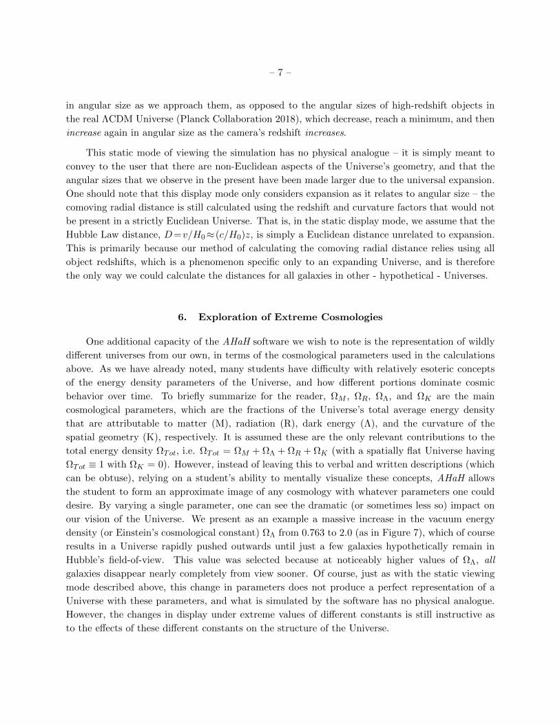
the application due to technical limitations. An example of the standard display mode is shown in
Figure 3.
When we move the camera to a certain position in the HUDF (X, Y, Z) data cube, we are
in general viewing the Universe as it would appear from that point and at that redshift. We
must qualify this statement by noting that the simulation accounts only for cosmological effects of
changing the camera position – no other dynamical, gravitational lensing, evolutionary, or other
cosmological or physical effects are simulated. In this sense, AHaH thus truly, though hypotheti-
cally, allows the user to travel through the Universe at “hyper-speed.” The highest virtual speed of
∼500×1012 times the speed of light that AHaH uses to zoom into the HUDF database allows the
observer to travel from z=0 to z<∼ 6 in a fraction of a minute, rather than in the ∼12.9 Gyr needed
if the maximum “travel” speed were really limited to the speed of light c, as in the real Universe.
As is covered in many introductory physics and astronomy classes, we use the Euclidean small
angle approximation (SAA), where for a fixed object length l and a small angle θ:
θ = tan(l
D) ≈ l
D, (2)
where the distance to the object is D. In relativity, we use essentially the same equation, but
replace D with DA, where DA is a complex function of redshift with a maximum at z ≈ 1.65. Thus
the relativistic SAA is:
θ ≈ l
DA. (3)

– 6 –
The somewhat counter intuitive relationship between an object’s angular size and its redshift in
Relativistic Cosmology is readily apparent in the standard display mode. If a user slowly increases
the redshift of the camera, high redshift objects will begin to decrease in angular size and move
toward the center of the display, eventually reaching a minimum angular size (at redshift z'1.65
in standard ΛCDM cosmology (Planck Collaboration 2018)), and then increasing. Also visible are
the effects of galaxy evolution and merging over time. For example, when viewing the Universe
from redshift z = 0.5 as in Figure 3, there are many large spiral and elliptical galaxies visible.
Note how the Universe is dominated by luminous red, early-type galaxies at moderate redshifts of
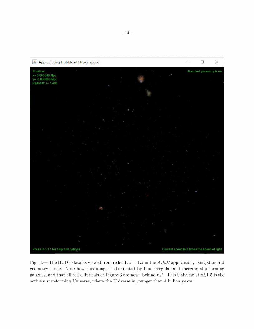
z<∼ 1 in Figure 3. However, when viewing the Universe from redshift z = 1.5 as in Figure 4, the
AHaH screen is dominated by small and compact blue galaxies. When zooming into the data at
z>∼ 1.5, many of these objects are blue irregular, merging and/or star-forming galaxies. In Figure 4,
all red ellipticals of Figure 3 are now “behind us”. This Universe at z>∼ 1.5 is indeed the actively
star-forming Universe, i.e., the first 4 billion years after the Big Bang.
It should be noted that the application does not make calculations for cosmological surface
brightness dimming or changes in color due to redshift or spectral evolution. While certainly
feasible to simulate, performing such image manipulation techniques on large numbers of galaxies
in real-time is currently too difficult for consumer computers. Moreover, we must also recall that
the HUDF data are limited in both magnitude and effective horizon by what could be observed
from low Earth orbit. When we view the data from redshifts other than zero, we would expect
to see more galaxies overall – including fainter galaxies – than are present in the current HUDF
data. We could choose to simulate these objects as extensions of our data set if desired, but we felt
this would not be particularly instructive, and could lead to potential confusion, as fainter galaxies
would have to be continuously simulated in increasing numbers by the computer below Hubble’s
detection limit when traveling from z=0 today to z<∼ 6 (∼1 Gyr after the Big Bang). Moreover, such
simulations have a high degree of uncertainty, and by significantly increasing the size of the data
set, would add prohibitively to the computation times. Likewise, we have chosen not to simulate
galaxies outside of the original field, which would of course enter the camera’s field of view as the
user pans around.
5. Static Geometry Mode
When a user presses the “G” key in the AHaH Java tool, they are told that they are viewing
the simulation with “unexpanding angular geometry” turned on. What this means specifically is
that angular sizes as derived above are no longer affected by the scale factor or curvature of the
Universe. After we develop our original coordinates, as in Equation (13), all calculations for angles
are simply done with θ=θE . This has the visual effect of all galaxies appearing smaller and closer
to the center of the viewport, since all initial angles have been contracted by an expansion factor of
(1+z) (when the curvature energy density ΩK is zero; see § 6 for an explanation of the main energy
densities at play in Relativistic Cosmology). In this static case, galaxies will also simply increase
– 7 –
in angular size as we approach them, as opposed to the angular sizes of high-redshift objects in
the real ΛCDM Universe (Planck Collaboration 2018), which decrease, reach a minimum, and then
increase again in angular size as the camera’s redshift increases.
This static mode of viewing the simulation has no physical analogue – it is simply meant to
convey to the user that there are non-Euclidean aspects of the Universe’s geometry, and that the
angular sizes that we observe in the present have been made larger due to the universal expansion.
One should note that this display mode only considers expansion as it relates to angular size – the
comoving radial distance is still calculated using the redshift and curvature factors that would not
be present in a strictly Euclidean Universe. That is, in the static display mode, we assume that the
Hubble Law distance, D=v/H0≈(c/H0)z, is simply a Euclidean distance unrelated to expansion.
This is primarily because our method of calculating the comoving radial distance relies using all
object redshifts, which is a phenomenon specific only to an expanding Universe, and is therefore
the only way we could calculate the distances for all galaxies in other - hypothetical - Universes.
6. Exploration of Extreme Cosmologies
One additional capacity of the AHaH software we wish to note is the representation of wildly
different universes from our own, in terms of the cosmological parameters used in the calculations
above. As we have already noted, many students have difficulty with relatively esoteric concepts
of the energy density parameters of the Universe, and how different portions dominate cosmic
behavior over time. To briefly summarize for the reader, ΩM , ΩR, ΩΛ, and ΩK are the main
cosmological parameters, which are the fractions of the Universe’s total average energy density
that are attributable to matter (M), radiation (R), dark energy (Λ), and the curvature of the
spatial geometry (K), respectively. It is assumed these are the only relevant contributions to the
total energy density ΩTot, i.e. ΩTot = ΩM + ΩΛ + ΩR + ΩK (with a spatially flat Universe having
ΩTot ≡ 1 with ΩK = 0). However, instead of leaving this to verbal and written descriptions (which
can be obtuse), relying on a student’s ability to mentally visualize these concepts, AHaH allows
the student to form an approximate image of any cosmology with whatever parameters one could
desire. By varying a single parameter, one can see the dramatic (or sometimes less so) impact on
our vision of the Universe. We present as an example a massive increase in the vacuum energy
density (or Einstein’s cosmological constant) ΩΛ from 0.763 to 2.0 (as in Figure 7), which of course
results in a Universe rapidly pushed outwards until just a few galaxies hypothetically remain in
Hubble’s field-of-view. This value was selected because at noticeably higher values of ΩΛ, all
galaxies disappear nearly completely from view sooner. Of course, just as with the static viewing
mode described above, this change in parameters does not produce a perfect representation of a
Universe with these parameters, and what is simulated by the software has no physical analogue.
However, the changes in display under extreme values of different constants is still instructive as
to the effects of these different constants on the structure of the Universe.
– 8 –
7. Integration in the Classroom and Lessons Learned
(Section to be completed based on usage in the classroom in Fall 2020):
In order to test the effectiveness of this software in a real education environment, we conducted
a study in astronomy classes at Arizona State University in the fall semester of 2020, as well as
a brief pilot study in a prior 2020 summer class. It should be noted that due to the outbreak
of COVID-19, ASU classes were moved into a partially online Synchronous format for all of the
summer 2020 semester and part/all of the fall 2020 semester, thus introducing an additional variable
as compared to a typical semester. This pandemic underlines the necessity of developing online
laboratory tools which complement virtual instruction, thus we felt continuing with our study was
particularly appropriate.
7.1. Methods
We selected the introductory astronomy lab for non-majors (AST 113/114 Summer-Fall 2020)
for our study in order to focus on the target population mentioned above - students first being
introduced to this type of astronomy content.
7.2. Analysis and Results
8. Other Program Uses
In addition to in the classroom, AHaH has been and continues to be useful in a wide range
of applications in STEM education. We have conducted several pilot programs to use this tool in
outreach efforts through several events held on and about ASU campus. As in education, while
static images have utility in outreach efforts with the general public, people young and old are
far more likely to become and stay engaged with dynamic media, such as simulation. As previous
studies have shown (e.g. Holzinger et al. 2008), simple dynamic media can improve the acquisition
and retention of information. In the case of interactive simulation like AHaH, this is likely because
the user becomes directly involved in shaping the course of their experience. In our program, this
is exemplified by members of the public being able to pick out the galaxies they ”fly” towards using
AHaH, and can learn more details about these. These programs have shown a qualitative increase in
participation by the general public in outreach activities, especially among young children or young
adults. As many public educators will attest, half the battle is often getting the public to start
using to an education opportunity. Thus the use of AHaH in the classroom is worth consideration
by teachers, outreach developers, and organizers.

– 9 –
9. Conclusion
We believe that our AHaH software provides students and instructors with an unprecedented
ability to interactively visualize many of the effects of a relativistically expanding Universe, among
its other capabilities. The application should help clarify these concepts, and allow students to
develop a deeper intuitive understanding of the material. Certain cosmological effects – such as
bandpass shifting, k-correction, surface brightness dimming, gravitational lensing, and the effects of
the magnitude limit and object sizes on the sample completeness limit – have been largely omitted
due to computational limitations, but we believe these to be not essential for the understanding
of the included effects. For a discussion of these more technical effects, see e.g., Windhorst et
al. (2018). In addition, our brief study of the utility of the program in the classroom meets our
expectations of its impact on learning, and lends support to our recommendation that further
virtual tools be developed in support of online classrooms. We also recommend the use of this tool
in other public education and science outreach efforts for its utility in quickly engaging the public.
For the convenience of those who wish to see or modify the particular implementation of
the above formulae within the Java software, we have provided source code with the standard
distribution of the tool. It is included in the src/ directory of ahah.jar, and may be extracted
using the java jar utility or any zlib-compatible de-compressor such as unzip. The tool may
be downloaded from the AHaH website12. Further details on AHaH download instructions and
installation are given in § 11 (Appendix B).
We thank Dr. Ned Wright for helpful discussion early in the project. We acknowledge student
support from the Arizona State University NASA Space Grant (to LJN and MRM). We acknowl-
edge support from Hubble Space Telescope grants HST-GO-10530.07-A, HST-GO-13779.005-A,
HST-EO-10530.25-A and HST-EO-13241.001-A from STScI, which is operated by AURA for NASA
under contract NAS 5-26555. RAW acknowledges support from NASA JWST Interdisciplinary Sci-
entist grants NAG-12460, NNX14AN10G and 80NSSC18K0200 from GSFC. Much of our education
design was based in part on the work by Hasper et al. (2015).
REFERENCES
Beckwith, S. V. W., et al. 2006, Astron. J., 132, 1729
Bertin, E., & Arnouts, S. 1996, Astron. & Astroph. Suppl. Ser., 117, 393
Bertin, E., Mellier, Y., Radovich, M., et al. 2002, Astronomical Data Analysis Software and Systems
XI, 281, 228
12http://ahah.asu.edu
– 10 –
Bolzonella, M., Miralles, J.-M., & Pello, R. 2000, Astron. & Astroph., 363, 476
Bouwens, R. J., Illingworth, G. D., Blakeslee, J. P., & Franx, M. 2006, Astrophys. J., 653, 53B
Cohen, S. H., Ryan, R. E. Jr., Straughn, A. N., et al. 2006, Astrophys. J., 639, 731
Dahlen, T., Mobasher, B., Dickinson, M., Ferguson, H. C., Giavalisco, M., Kretchmer, C., Ravin-
dranath, S., 2007, Astrophys. J., 654, 1
Hasper, E., Windhorst, R. A., Hedgpeth, T., et al. 2015, J. College Sc. Teaching, 44, 82
Hoeling, B. 2012, American Journal of Physics 80, 334
Holzinger, A., Kickneier-Rust, M., & Dietrich, A. 2008, Educational Technology & Society, 11
Longair, M. S. 1998, Galaxy Formation (Berlin: Springer-Verlag)
Lupton, R., Blanton, M. R., Fekete, G., Hogg, D. W., O’Mullane, W., Szalay, A., & Wherry, N.
2004, Publ. Astron. Soc. Pac., 116, 133
Pirzkal, N., Xu, C., Malhotra, S., et al. 2004, Astrophys. J. Suppl. Ser., 154, 501
Pirzkal, N., Malhotra, S., Ryan, R. E., et al. 2017, Astrophys. J., 846, 84
Planck Collaboration: Aghanim, N., Akrami, Y., Ashdown, M., et al. 2018, Astron. & Astroph.
(https://arxiv.org/abs/1807.06209v2)
Retzlaff, J., Rosati, P., Dickinson, M., Vandame, B., Rite, C., Nonino, M., Cesarsky, C., the
GOODS Team, 2010, Astron. & Astroph., 511
Ryan, R. E., Jr., Hathi, N. P., Cohen, et al. 2007, Astrophys. J., 668, 839
Ryden, B. 2017, Introduction to Cosmology, 2nd Edition Cambridge University Press (Cambridge,
United Kingdom)
Sadaghiani, H. 2011, Phys. Rev. ST Phys. Educ. Res. 7, 010102
Thompson, R. I., et al. 2005, Astron. J., 130, 1
Windhorst, R. A., Hathi, N. P., Cohen, S. H., et al. 2008, J. Adv. Space Res., 41, 1965
Windhorst, R. A., Cohen, S. H., Hathi, N. P., et al. 2011, Astrophys. J. Suppl. Ser. 193, 27
Windhorst, R. A., Timmes, F. X., Wyithe, J. S. B., et al. 2018, Astrophys. J. Suppl. Ser. 234, 41
Wright, E. L. 2006, Publ. Astron. Soc. Pac., 118, 1711
Yan, H. & Windhorst, R. A. 2004, Astrophys. J., 612, L93a
This preprint was prepared with the AAS LATEX macros v5.2.

This page intentionally left blank.
11

– 12 –
Fig. 1.— A comparison of three images of HUDF galaxy 7556. The left image is that from the
original STScI release, clearly showing the bright, burned-out knots characteristic of the standard
logarithmic image stretch. The center image is our prepared image using the arcsinh stretch de-
scribed by Lupton et al. (2004), as it appears in the AHaH application. The right image is our
prepared image against an artificially imposed chessboard pattern, showing the included trans-
parency. Note that pixels outside the source are all completely transparent, since they have been
removed entirely using the SourceExtractor segmentation map.
Fig. 2.— Our prepared images of three galaxies from the HUDF, using the arcsinh stretch described
by Lupton et al. (2004). Shown are galaxy 3180 (left), galaxy 5805 (center), and galaxy 6974 (right).
– 13 –
Fig. 3.— The HUDF data as viewed from redshift z = 0.5 in the AHaH application, using standard
geometry mode, which properly calculates angular sizes. Note how the image is dominated by
luminous red early-type galaxies at moderate redshifts of z<∼ 1, where the Universe is older than 6
billion years.
– 14 –
Fig. 4.— The HUDF data as viewed from redshift z = 1.5 in the AHaH application, using standard
geometry mode. Note how this image is dominated by blue irregular and merging star-forming
galaxies, and that all red ellipticals of Figure 3 are now “behind us”. This Universe at z>∼ 1.5 is the
actively star-forming Universe, where the Universe is younger than 4 billion years.

– 15 –
Fig. 5.— The HUDF data as viewed from redshift z = 0 in the AHaH application, using standard
geometry mode. This displays the entire HUDF, for comparison with Figures 6 and 7.

– 16 –
Fig. 6.— The HUDF data as viewed from redshift z = 0 in the AHaH application, using static
geometry mode. This displays the entire HUDF, and one can see the evident ”contraction” of the
field of galaxies due to the lack of non-Euclidean geometry in the real HUDF data. (That is, the
HUDF data in a relativistically expanding cosmology — when shown in Euclidean geometry —
compresses all objects towards the image center, since the square cylindrical volume is now not
undergoing the expansion, as it should).

– 17 –
Fig. 7.— The HUDF data as viewed from redshift z = 0 in the AHaH application, using standard
geometry mode, with a vacuum energy density parameter ΩΛ value increased from the default
value of 0.763 to 2.0. One can see that the extreme value causes most galaxies that are visible in
the standard ΛCDM cosmology (Planck Collaboration 2018) to disappear due to vastly increased
expansion in this case. This value was selected because noticeably higher values of ΩΛ cause all
galaxies to disappear entirely - we observers likely live in a reletivistic Universe with a ”little
Lambda.”

– 18 –
10. Appendix A. Derivation of Equations
Here we include our derivations of the math used in AHaH at a level appropriate for an
intermediate undergraduate cosmology class13.
10.1. Comoving Radial Distance
To begin, we need the comoving radial distance, DR, from the Earth to an object at redshift
z, derived from the Robertson-Walker metric, as discussed previously, e.g., Longair (Ch. 7 1998),
Eqs. 5.33 and 6.13 of Ryden (2017), and Eq. 6 of Wright (2006). We express this as the integral:
DR(z) =
∫ t0
t
c · dta
=
∫ 1
11+z
c · daaa
=c
H0
∫ z
0
dz
(1 + z)a, (4)
where the scale factor a = 1/(1 + z). The derivative of a with respect to time, a, is given by the
expression:
a = (ΩM/a+ ΩR/a2 + ΩΛ · a2 + ΩK)1/2, (5)
where ΩM , ΩR, ΩΛ, and ΩK are energy density parameters, corresponding to the fractions of the
Universe’s total average energy density that are attributable to matter (M), radiation (R), dark
energy (Λ), and the curvature of the spatial geometry (K), respectively. Note that it is assumed
these are the only relevant contributions to the total energy density ΩTot. That is, we assume that
ΩTot = ΩM + ΩΛ + ΩR + ΩK . A spatially flat Universe would have ΩTot ≡ 1 with ΩK = 0. The
default Planck Collaboration (2018) parameters used are: Ho = 68 km/sec/Mpc, ΩM = 0.32, ΩΛ
= 0.68, ΩR = 9×10⁻⁵ with ΩK = 0.
We evaluate this integral in steps of 0.05 in z from z = 0 to z = 20 to create a look-up table,
interpolating linearly to find the value for any arbitrary redshift in between these discrete steps.
This is because we must make the calculation frequently and for many objects, so computing the
integral manually every time would be computationally prohibitive. The resulting error in this
method is generally small enough that it translates to less than one pixel’s difference even on high-
resolution displays, so this error can safely be ignored for the purposes of the application. We
evaluate the integral using the simple midpoint method, which may not be the optimal solution,
but was simple to implement and adequately efficient on any home computer. As with the linear
interpolation, higher accuracy numerical integration would result in less than one pixel’s difference
when displayed.
13See, e.g., http://windhorst322.asu.edu
– 19 –
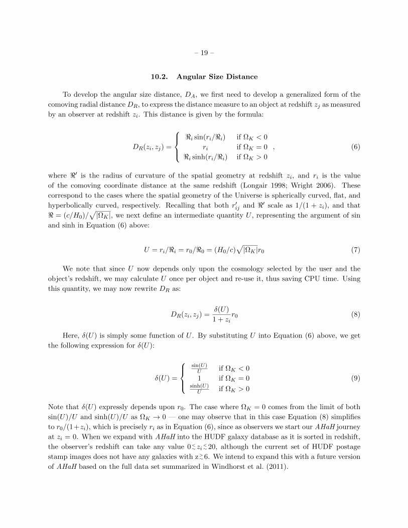
10.2. Angular Size Distance
To develop the angular size distance, DA, we first need to develop a generalized form of the
comoving radial distanceDR, to express the distance measure to an object at redshift zj as measured
by an observer at redshift zi. This distance is given by the formula:
DR(zi, zj) =
<i sin(ri/<i) if ΩK < 0
ri if ΩK = 0
<i sinh(ri/<i) if ΩK > 0
, (6)
where <′ is the radius of curvature of the spatial geometry at redshift zi, and ri is the value
of the comoving coordinate distance at the same redshift (Longair 1998; Wright 2006). These
correspond to the cases where the spatial geometry of the Universe is spherically curved, flat, and
hyperbolically curved, respectively. Recalling that both r′ij and <′ scale as 1/(1 + zi), and that
< = (c/H0)/√|ΩK |, we next define an intermediate quantity U , representing the argument of sin
and sinh in Equation (6) above:
U = ri/<i = r0/<0 = (H0/c)√|ΩK |r0 (7)
We note that since U now depends only upon the cosmology selected by the user and the
object’s redshift, we may calculate U once per object and re-use it, thus saving CPU time. Using
this quantity, we may now rewrite DR as:
DR(zi, zj) =δ(U)
1 + zir0 (8)
Here, δ(U) is simply some function of U . By substituting U into Equation (6) above, we get
the following expression for δ(U):
δ(U) =
sin(U)
U if ΩK < 0
1 if ΩK = 0sinh(U)
U if ΩK > 0
(9)
Note that δ(U) expressly depends upon r0. The case where ΩK = 0 comes from the limit of both
sin(U)/U and sinh(U)/U as ΩK → 0 — one may observe that in this case Equation (8) simplifies
to r0/(1+zi), which is precisely ri as in Equation (6), since as observers we start our AHaH journey
at zi = 0. When we expand with AHaH into the HUDF galaxy database as it is sorted in redshift,
the observer’s redshift can take any value 0<∼ zi
<∼ 20, although the current set of HUDF postage
stamp images does not have any galaxies with z>∼ 6. We intend to expand this with a future version
of AHaH based on the full data set summarized in Windhorst et al. (2011).

– 20 –
Thus, using our Equation (8) and the equation relating the angular size distance and the
distance measure as developed by Longair (1998, Eq. 7.50), the angular size distance from redshift
zi to zj is given by:
DA(zi, zj) = DR(zi, zj)1 + zi1 + zj
=δ(U)
1 + zjr0 (10)
10.3. Comoving Coordinate System
Now that we have developed formulae for DR and DA, we can consider the best way to create
a coordinate system for the Java application. The data we start with are the redshift zj of object j
(with which we can calculate DR) and four angles: the object’s angular size (from the height and
width of its image) and the angular separation between the object and the x and y axes, which
we define as lines going through the center of the original image. These angles are calculated by
taking the corresponding size in pixels and multiplying by the scale in arcsec/pixel of the original
HST image14.
We would like to use this information to create a coordinate system with the original telescope
position at the origin. In a Euclidean space this would present no problem, but we have already
remarked that the observed angles are not the same in an expanding Universe as they would be in a
Euclidean space. Further, it would be desirable for the Euclidean coordinate distance to correspond
to the comoving radial distance, as this would make calculations significantly simpler. We can
accomplish this, but when we create coordinates for each object as such, we need to “correct” the
observed angles. That is, we want a “Euclidean angular size” associated with a certain observed
angular size. We will call this θE . An object’s angular size is related to its physical transverse
diameter, d, by the following equation which derives from Equation (10):
d = θDA = θδ(U)
1 + zjr0 = θE
1
1 + zir0 (11)
Note that in the Euclidean case we must contract r0 by a factor of 1/(1 + zi) to get the comoving
distance from zi to zj as measured by the observer at zi (ri in Equation (6) above). This is because
the proper spatial separation in the current epoch has been stretched by the Universe’s expansion,
so as seen by an observer at redshift zi it must be scaled appropriately. Hence, the equivalent
Euclidean distance between any two points is DE = r0/(1 + zi), in which case we get the Euclidean
small-angle approximation back: d = θEDE .
Thus canceling r0, we get the following expression for θE from Equation (11):
14The HUDF mosaics used have been drizzled to a scale of 0′′.03 per pixel

– 21 –
θE = θδ(U)1 + zi1 + zj
(12)
In our initial data zi is simply zero, so that we create coordinates (X, Y , Z) for an object at redshift
z like:
X = sin
(δ(U)θX1 + z
)cos
(δ(U)θY1 + z
)DR(0, z), (13)
and similarly for Y and Z. We have thus developed a coordinate system of X, Y , and Z in comoving
Mpc with the original telescope position at the origin.
10.4. Simulating Observations From Vantage Points Other Than z = 0
Now, when we “move” the Hubble camera virtually to higher redshifts, we do so by moving to some
new (Xc, Yc, Zc) value in the coordinate space. (Note that AHaH does not only “virtually violate
the laws of physics” by moving the observer into the HUDF images at ∼500×1012 times the speed
of light, but it also has no problem “violating the arrow of time” by allowing the user to move back
and forth in redshift through the sorted HUDF image data cube). By construction, the distance
measure here is just the Euclidean coordinate distance:
DE = ((X −Xc)2 + (Y − Yc)2 + (Z − Zc)
2)1/2 (14)
Now to determine where to display an object after we have “moved” the camera, we use the distance
calculated with Equation (14) and the Euclidean angular size. Using the redshift of the object of
interest, zo, and the camera’s user-defined redshift, zc, we rearrange Equation (12) to get:
θ = θE1 + zo
δij(1 + zc)(15)
Here δij follows from Equation (6) and Equation (9) for an object at redshift zj as observed from
redshift zi. In this case, θE is a quantity that we must calculate from our coordinates in the usual
Euclidean way.
For an object’s angular size it is even simpler than for its (X,Y, Z) position, since we do not
have to manually calculate θE . We know that in the Euclidean case:
d = θ0DR = θEDE , (16)

– 22 –
where θ0 is the Euclidean angular size from redshift zero, and DE is the coordinate distance from the
camera to the object from Equation (14). We then solve for θE in Equation (16), θE = θ0DR/DE ,
and substitute back into Equation (15) to obtain an expression for the desired angular size θ for
any object at redshift zo as observed from zc:
θ = θ0
(DR
DE
)1 + zo
δij(1 + zc)(17)
11. Appendix B. AHaH User Manual
For completeness and convenience of the AHaH user, we summarize here the basic AHaH Users
Manual as it is currently available on the AHaH website:
1 * System Requirements
2 * Installing and Running the Application
3 * Main Screen and User Interface
4 * Moving the Camera
5 * Hot keys and Special Functions
6 * Changing Options and Settings
7 * Configuration File and Advanced Options
8 * License, Source Code, and Modifications
9 * Additional Instructions for Mac Users
1 * System Requirements
The following are the minimum system requirements to run the Appreciating
Hubble at Hyper-speed application:
* Microsoft Windows, Mac OS, or *nix operating system with Sun Java
run time version 1.4.3 or later
* 1.0 GHz processor
* 256 MB RAM
* Mouse and Keyboard
We recommend the following for optimal system performance:
* 2.0 GHz dual-core processor
* 1.0 GB RAM
* Graphics accelerator card with 64 MB video RAM

– 23 –
In addition, an internet connection is required if the user wishes to view
extended information about selected galaxies.
2 * Installing and Running the Application
The Appreciating Hubble at Hyper-speed application is distributed as an
archive containing a standard executable Java resource file. To install the
application, simply download the archive file for the user’s operating
system and save it wherever preferred. Extract the archive wherever desired,
and then double-click the ahah.jar file to run the program. If the user
prefers to run from the command line, then simply use: java -jar ahah.jar
For further details on the installation, see subsection 9 below.
Also provided is a configuration file, ahah.conf, that provides several
options that the user may modify if the user wants to use custom settings
every time they run the program. See the Configuration File section for more
information.
3 * Main Screen and User Interface
The main screen represents the user’s primary interface with the application.
Besides holding the actual visualization, the screen also provides various
forms of information about the simulation and methods to interact with and
gain more information about specific galaxies.
The numbered user interface elements are as follows:
1. Position Indicator, showing the camera’s x and y position within the
coordinate system, as well as the camera’s redshift.
2. Active Geometry Indicator, showing whether the Universe’s real
geometry is active or a non-physical geometry, in which angular
sizes are unaffected by the Universe’s expansion.
3. Info Box that shows more information about the selected galaxy,
including its HUDF ID, redshift, and comoving radial distance.
4. Jump Dialog, where the user may enter an Object ID or redshift on
which to center the camera.
5. Speed Indicator. Used to remind the user that the speeds represented
in the application (when moving) are not physically attainable.
4 * Moving the Camera

– 24 –
The user may move the camera using either the mouse or keyboard, or with a
combination of both. We recommend that most users navigate with the mouse,
though advanced users may find the precision movement afforded by the
keyboard useful in some situations.
To navigate using the mouse, simply click and hold the left mouse button
anywhere within the Main Screen. Moving the mouse will then move the camera
left, right, up, and down. To move forward and backward, either scroll the
mouse wheel up and down, or click and hold the mouse wheel or middle mouse
button, then move the mouse forward and backward. The user may also move
forward and backward by holding shift while clicking and holding the left
mouse button.
To navigate using the keyboard, simply use the arrow keys to move left,
right, up, and down. To move forward and backward, hold shift and use the up
and down arrow keys. Holding control while using keyboard navigation will
move the camera at 10x the normal speed.
In addition to direct navigation, the user may double left-click on any
galaxy to initiate an automatic move to it. This will move the camera at
a moderate pace along the line (geodesic) between the camera and the
galaxy. The automatic move can be canceled at any time by performing most
other actions, such as attempting to move the camera or selecting a galaxy.
Note that toggling the spatial geometry mode will not cancel an automatic
movement.
5 * Hot keys and Special Functions
The application contains a number of additional features besides moving the
camera, most of which are accessed using hot keys. The following table
contains an overview of these additional features and their hot keys:
Program Feature: Hot keys
Select a galaxy and open its Info Box: Left-click galaxy
Toggle spatial geometry mode: G
Open Jump Dialog to travel to a specific galaxy/redshift: J
Reset the simulation and move the camera to the origin: R or F5
Open the Help and Options Dialog: H or F1

– 25 –
Info Box
The Info Box contains various information about the selected galaxy:
* The Object ID is a number uniquely identifying each galaxy and can be
used in conjunction with the Jump Dialog to direct another user to a
specific galaxy.
* The Redshift represents the factor by which a galaxy’s observed
spectrum is shifted from what we would observe if it were nearby.
It is this measurement that allows us to calculate distances to
galaxies using Hubble’s law.
* The Comoving Radial Distance represents the spatial separation of the
galaxy from the origin at the present epoch, assuming zero peculiar
velocity with respect to our own galaxy. It is calculated using the
currently active cosmology constants.
* The Stamp Size is the length of one side of the black box surrounding
the galaxy’s picture. Thus if a galaxy takes up roughly half the
width of the box and has a stamp size of 30 kpc, its proper
transverse diameter should be about 15 kpc.
* The More Information Link links to a web page containing additional
data for the selected galaxy. This includes its position (J2000 RA
and Dec coordinates) and spectral fitting data. Note that not all
galaxies have this additional information available. Specifically,
it is available only for those galaxies that were included in the
GRAPES survey, which are most of the brighter, larger galaxies.
* The Jump Button moves the camera to a view centered on the selected
galaxy, exactly as if the galaxy’s ID number had been entered into
the Jump Dialog.
Spatial Geometry Mode
Toggling the spatial geometry mode changes between the Universe’s actual
geometry and a geometry where angular sizes are unaffected by the expansion
of the Universe. This second geometry does not have a physical analogue - it
does not represent what the Universe would look like if it were not
expanding, or any other such set of circumstances. Instead, it is provided
simply to convey visually that observed angular sizes have been affected by
the scale factor.
Jump Dialog

– 26 –
The Jump Dialog is a way to quickly move to a specific location. If the user
enters an Object ID number, then the simulation will move the camera to a
position centered on that object. This is useful for labs that require
students to examine a number of specific galaxies. If no Object ID is
entered then the simulation will move the camera to the specified redshift,
leaving the x and y coordinates fixed.
Resetting
Using the reset function will reset the simulation, exactly as if the
application had been newly opened. This includes reloading all galaxies -
both images and position data - as well as recalculating all distances and
moving the camera to the origin. It also resets the graphics rendering
thread, so may be used in the event that images fail to update.
Help and Options Dialog
The Help and Options Dialog gives the user basic information about running
the application, such as movement controls, as well as allowing the user to
modify some of the simulation’s configuration parameters at run time. It is
discussed in detail in the next section. In addition, the license for the
software is also provided in this dialog.
6 * Changing Options and Settings
There are two primary ways of changing options and settings for the
application. These are the Configuration File, which will be covered in the
next section, and the options pane of the Help and Options Dialog. The
options pane contains two primary sections, Cosmology Parameters and Program
Performance.
Cosmology Parameters
The Cosmology Parameters section allows the user to modify certain constants
of the displayed cosmology. There are currently four parameters that may be
modified at run time:
* H0 is the Hubble Constant, which goes into Hubble’s Law v = H0*D relating
recessional velocity v and distance D. It is also used when obtaining
– 27 –
proper distances from coordinate distances within the application.
Its units are km/s/Mpc.
* OmegaM is the matter density parameter of the Universe. It represents what
fraction of the total energy density of the Universe is attributable
to matter, both baryonic and dark. The Planck (2018) value is
OmegaM = 0.32.
* OmegaLambda is the so-called vacuum energy density parameter of the
Universe. It represents what fraction of the total energy density of the
Universe is attributable to dark energy, ie. expansion energy
associated with the Cosmological Constant, Lambda. The Planck (2018) value
is OmegaLambda = 0.68.
* OmegaR is the radiation density parameter of the Universe. It represents
what fraction of the total energy density of the Universe is
attributable to radiation.
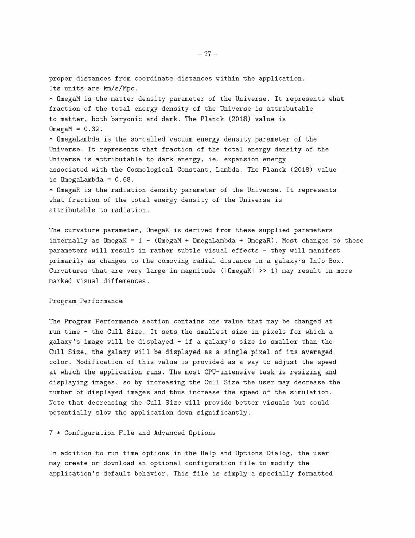
The curvature parameter, OmegaK is derived from these supplied parameters
internally as OmegaK = 1 - (OmegaM + OmegaLambda + OmegaR). Most changes to these
parameters will result in rather subtle visual effects - they will manifest
primarily as changes to the comoving radial distance in a galaxy’s Info Box.
Curvatures that are very large in magnitude (|OmegaK| >> 1) may result in more
marked visual differences.
Program Performance
The Program Performance section contains one value that may be changed at
run time - the Cull Size. It sets the smallest size in pixels for which a
galaxy’s image will be displayed - if a galaxy’s size is smaller than the
Cull Size, the galaxy will be displayed as a single pixel of its averaged
color. Modification of this value is provided as a way to adjust the speed
at which the application runs. The most CPU-intensive task is resizing and
displaying images, so by increasing the Cull Size the user may decrease the
number of displayed images and thus increase the speed of the simulation.
Note that decreasing the Cull Size will provide better visuals but could
potentially slow the application down significantly.
7 * Configuration File and Advanced Options
In addition to run time options in the Help and Options Dialog, the user
may create or download an optional configuration file to modify the
application’s default behavior. This file is simply a specially formatted
– 28 –
text file called ahah.conf that must be placed in the same directory as
ahah.jar. The options are placed in the file as Key : Value pairs separated
by a colon. For example the line OmegaM : 0.32 sets OmegaM to 0.32, the
currently accepted Planck (2018) value. Comments within the file are preceded by
# and section headings (optional) are placed in brackets, such as [Cosmology
Constants]. Keys other than those below will simply be ignored, and giving a
key an improper value (such as a floating point number where an integer is
required) will cause the application to print an error and then use the
default value. The available options are as follows:
Application Operation Options
Options in this section change the default behaviors of how the application
runs, including performance tweaks. If AHaH is to be shown to students that
are taught over the internet via a Zoom-like application, this parameter has
to be chosen judiciously, as the demonstrated performance of AHaH will now
be limited by the local internet speed, and not the host’s computer speed.
* FrameSleepTime is an integer that specifies the time in milliseconds
to wait between redraws of the main simulation window. A shorter
time will update the viewport more often, but be more taxing on the
CPU. Modifying the default value may affect performance drastically.
* MacroStepDelay is an integer that specifies the time in milliseconds
to wait between steps of an automatic move (when double-clicking on
a galaxy). A shorter time will result in smoother, faster movement.
* CullSize is an integer that specifies the default Cull Size, as
discussed in the Options and Settings section above. This way if the
user has a particularly fast computer, they can force the
application to use a smaller Cull Size every time they run it. Thus
the user would not have to open the Help and Options Dialog to
change it every time. Note that modifying the value at run time
using the Help and Options Dialog will always override any value in
the configuration file.
* DefaultBrowser is a string representing the user’s preferred browser
command on any Unix or Linux systems. If the user does not change
this setting themselves, the application will try, in order the
following browsers: firefox, mozilla, opera, konqueror, epiphany,
netscape. The value set in the configuration file is simply any
shell command, so may be something in $PATH like firefox, or the
full path such as: /usr/local/share/firefox/firefox. On Windows
– 29 –
and Mac OS, the operating system’s default browser is always used,
so modifying this setting will have no effect.
Cosmology Constants
Options in this section set the defaults for various cosmology constants.
For more detailed explanations, see the descriptions for the parameters in
the Options and Settings section above. Like the Cull Size, changing the
values at run time using the Help and Options Dialog will override settings
in the configuration file. The default Planck (2018) parameters are: H0 = 68
km/sec/Mpc, Omega_M = 0.32, Omega_Lambda = 0.68, and Omega_R = 9 x 10^-5.
* HNought is a floating point number that specifies the default value of
the Hubble Constant, H0.
* OmegaM is a floating point number that specifies the default value of
the matter density parameter, OmegaM.
* OmegaV is a floating point number that specifies the default value of
the vacuum energy density parameter, OmegaLambda.
* OmegaR is a floating point number that specifies the default value of
the radiation density parameter, OmegaR.
Dataset Information
Options in this section give the application information about the original
image that the individual stamps come from, as well as specifying where to
find the object database. Options from this section should generally not be
changed by users - they are provided for future use of the application with
different data.
* DBFile is a string representing the path of the database file within
the jar file. This should only be modified if the application is
repackaged with different data. The file should be specified with
the root of the path being the root of the jar file, not of the
computer’s file system.
* ImageSizePx is an integer specifying the height and width of the
original image in pixels. If for some reason the image is not
square, use whichever dimension is larger.
* ImageArcsecPerPx is a floating point number that specifies the
arcsec/pix scale of the original image. This is used internally for
changing pixel sizes to angular sizes and vice versa.
– 30 –
* MaxRedshift in an integer that specifies the maximum redshift for the
distance tables. This need only be sufficiently large such that no
object in the database has a higher redshift (as the program may
then crash since it would not be able to correctly interpolate the
object’s distance).
Application Configuration Constants
Options in this section change aspects of the application that users
generally do not need to modify, such as the locations of external resources
like this documentation. These options are provided primarily as a
convenience to website administrators in the event that URLs change, etc.
* StampURLBase is a string that specifies the directory containing the
More Information html files for galaxies. The provided string must
contain the trailing /. The application expects the html files
within this directory to be named n.html, where n is the HUDF ID
number of the object.
* HelpURL is a string that indicates the url of the application’s online
documentation, i.e. this page.
* TextColor is a hex code that defines the color of the text on the Main
Screen. The value is standard RGB hex encoding (like in HTML and
CSS), i.e. RRGGBB. For instance a deep purple would be encoded as
TextColor : 6633aa.
8 * License, Source Code, and Modifications
The Appreciating Hubble at Hyper-speed (AHaH) application is provided under a
BSD-like license. In simple terms, this means that virtually any
modification or redistribution of the application is permitted, with the
following caveats:
* Any redistribution must retain the original copyright notice and
license file, either with the source code or with the documentation
in the case of binary distributions.
* The names of the copyright holders, contributors, and associated
institutions may not be used to endorse or promote any derivative
works without prior permission.

– 31 –
Note that there is no requirement that source code be provided with any
derivative work or redistribution. We encourage any derivative works to
provide source code as well so that others may learn from the user’s
modifications, but we leave such decisions to the user’s discretion.
9.a Application Source Code (All OS, Mac Terminal Users)
The application’s source code is provided with the standard distribution.
Java archives are simply standard ZIP (DEFLATE) archives with a special
internal directory structure. Thus, the user only needs to extract the contents
of the archive using their favorite ZIP extractor. (Using jar, the user would
simply run: jar -xf ahah.jar ). The application source code is contained
in the src/ directory.
Warning: The ahah.jar file exhibits "tarbomb" behavior, extracting to the
current directory instead of its own subdirectory. This is mostly a
limitation of the jar format, since the META-INF/ directory must always be
in the archive root. We strongly recommend the user moves the archive to its own
directory before extracting it.
To compile the source the user simply needs to run in terminal mode:
javac *.java. The compiled binaries will automatically be placed within the
directory edu/asu/Ahah/. To run the modified application, the user then needs to
create a new jar including the directories edu/, images/, and data/, as well as
the files defaults.conf and license.txt, and any source code if the user desires.
The user also needs to specify a Manifest file, which must contain at least
the line Main-Class: edu.asu.Ahah.Ahah -- this tells the Java interpreter
where to find the main class when a user runs the jar. An example jar
creation command is:
jar -cvfm ahah.jar MANIFEST.MF edu images data src defaults.conf license.txt
9.b Application Source Code (Mac GUI Users)
Some users have reported some issues with launching AHaH from modern Mac
operating systems. We include here detailed instructions (as of OS 10.14.6)
for use of the tool. Note: the user must have administrative access to the
Mac in question - with full download rights.
* Download the ahah_Mac_iOS.zip file from the AHaH website (use the lower

– 32 –
download button)
* Double-click on the file, opening a new window with AHaH and the user’s
Applications folder
* Drag AHaH to the Applications folder, close this window
* Navigate to the Applications folder and control-click AHaH
* If the user gets any error other than the steps below, the user should try
to continue clicking through all errors to allow AHaH to run.
* If the user gets an error that the user needs the legacy version of Java,
close the error, navigate to java.com, and install Java
* Double-click again on AHaH in the Applications folder
* If a similar error occurs as before, click the now available more
information option
* This should bring the user to the legacy Java installation, which the user
should complete
* Double-click on AHaH again, and close the permissions error
* Navigate to the user’s System Preferences menu
* Navigate to the Security & Privacy submenu
* Where the page says AHaH was blocked from running, and click "Open Anyway"